Rice-like complexity lower bounds for
Boolean and uniform automata networks

Abstract

Automata networks are a versatile model of finite discrete dynamical systems composed of interacting entities (the automata), able to embed any directed graph as a dynamics on its space of configurations (the set of vertices, representing all the assignments of a state to each entity). In this world, virtually any question is decidable by a simple exhaustive search. We lever the Rice-like complexity lower bound, stating that any non-trivial monadic second order logic question on the graph of its dynamics is ${\mathsf{NP}}$-hard or ${\mathsf{coNP}}$-hard (given the automata network description), to bounded alphabets (including the Boolean case). This restriction is particularly meaningful for applications to “complex systems”, where each entity has a restricted set of possible states (its alphabet). For the non-deterministic case, trivial questions are solvable in constant time, hence there is a sharp gap in complexity for the algorithmic solving of concrete problems on them. For the non-deterministic case, non-triviality is defined at bounded treewidth, which offers a structure to establish metatheorems of complexity lower bounds.

1 Introduction

A natural way to formalize the intuitive notion of “complexity” arising in the dynamics of discrete dynamical systems employs the well established theory of algorithmic complexity. This approach has notably been carried on cellular automata [32, 14, 22, 25, 4], lattice gas [24, 20] and sandpile [23, 8], regarding the prediction of their dynamics. It has also been introduced on automata networks, a bioinspired model of computation on which the present work is grounded, with a particular focus on fixed points [1, 7, 27, 17].

Automata networks are a general model of interacting entities, where each automaton holds a state (taken among a finite alphabet), and updates it according to each other’s current state. In the deterministic setting, the behavior of each automaton is described by a local update function, which are all applied synchronously in discrete steps. In the non-deterministic setting, multiple concurrent behaviors are possible. The set of automata and states are finite, so is the configuration space (assigning a state to each automaton). The dynamics of an automata network is the graph of the transition function or relation on its configuration space. This model is very general, in the sense that any directed graph is the dynamics of some automata network (the graph has out-degree $1$ in the deterministic setting). Automata networks have applications in many fields, most notably for the modeling of gene regulation mechanisms and biological systems in general [16, 34, 18]. In this context, restricting the set of possible states of each automaton is particularly meaningful [6, 15, 21, 33, 18]. A prototypical example is the Boolean case, where each automaton holds a state among $\{0,1\}$. This is the constraint targeted in the present article. The consideration of alternative update modes is another central concern in the community (see [29] for a survey), here we stick to the synchronous case, also called the parallel update mode.

A pillar of computer science is Rice theorem [30]: any non-trivial semantic property of programs is undecidable. It is striking for its generality and the sharp dichotomy of difficulty between trivial and non-trivial problems. We look for analogs in this spirit. A finite discrete dynamical system can only ask decidable questions (simply because it is finite), hence we shift the perspective from computability to complexity theory. We lever the Rice-like complexity lower bounds of [9, 10], from succinct graph representations (where it contrasts Courcelle theorem) to natural models of interacting entities (automata networks on bounded alphabets). Such metatheorems are obtained using the expressiveness of graph logics, all at monadic second order (MSO) in the present work. A key consists in defining a notion of non-triviality as general as possible. It turns out to be a sharp and deep dichotomy in the deterministic case (AN) because trivial questions are answered in constant time. In the non-deterministic case (NAN), we employ a notion of non-triviality relative to dynamics of bounded treewidth, which we call arborescence (its necessity is addressed in [10], and discussed in the perspectives). Our results apply to uniform automata networks, where all automata are constrained to have the same alphabet size (denoted $q$). All the necessary concepts will be defined in the preliminary section. We gather our main results in one statement, where in bold is the problem consisting in deciding whether the dynamics of an automata network (given a description of the behavior of its entities) verifies some property $\psi$ expressed in graph logics.

Theorem 1.

Let $q\geq 2$ be any alphabet size for uniform automata networks.
Deterministic:
a. For any non-trivial MSO formula, $\psi$-AN-dynamics is ${\mathsf{NP}}$- or ${\mathsf{coNP}}$-hard.
b. For any $q$-non-trivial MSO formula, $\psi$-$q$-AN-dynamics is ${\mathsf{NP}}$- or ${\mathsf{coNP}}$-hard.
Non-deterministic:
c. For any arborescent MSO formula, $\psi$-NAN-dynamics is ${\mathsf{NP}}$- or ${\mathsf{coNP}}$-hard.
d. For any $q$-arborescent MSO formula, $\psi$-$q$-NAN-dynamics is ${\mathsf{NP}}$- or ${\mathsf{coNP}}$-hard.

Part c of Theorem 1 is proven in [10]. The ${\mathsf{NP}}$ and ${\mathsf{coNP}}$ symmetry is necessary in such a general statement, because some problems expressible at first order (such as the existence of a fixed point in the dynamics) are known to be ${\mathsf{NP}}$-complete [1], and the graph logics we consider are closed by complemention (simply by adding a negation on top of the formula). The proof technique nevertheless gives a clear characterization of which of these two lower bounds is proven for each formula $\psi$, through the concept of saturating graph (denoted $\Omega_{m}$ because it only depends on the quantifier rank $m$ of $\psi$) introduced in [10]. If $\Omega_{m}$ satisfies an MSO formula $\psi$, then the corresponding $\psi$-dynamics problem is proven to be ${\mathsf{NP}}$-hard, otherwise it is proven to be ${\mathsf{coNP}}$-hard.

In Section 2 we introduce all the necessary notions involved in the statement and in the proof of Theorem 1, including graph logics and tree-decompositions. Theorem 1 extends known results in two directions:

• generalizing to MSO the result of [9] in the deterministic case, by employing the abstract pumping technique based on finite model theory from [10],

• proving that the Rice-like complexity lower bounds also hold on $q$-uniform networks, where automata states are taken among a common alphabet of size $q\geq 2$.

The proof technique developed in [10], on which our extensions are grounded, is detailed in Section 3 where all the ingredients to design a polytime reduction from SAT are exposed. In Section 4 we apply the technique to deterministic dynamics, i.e. to graphs of out-degree $1$, and prove part a of Theorem 1. Section 5 is dedicated to the study of arithmetical considerations in order to obtain $q$-uniform dynamics (on a configuration space of size $q^{n}$ for some number $n$ of automata) when pumping a part of size $a$ from a graph of size $b$ (that is, obtaining potential dynamics of size $ak+b$ where $k$ is the number of copies of size $a$ which have been added to the initial graph of size $b$). We give a separate consideration to the Boolean case $q=2$, which is simpler and gives the intuitions for the last ingredients of our main results. In Section 6 we apply the arithmetics of the previous section to derive parts b and d of Theorem 1 which, to our point of view, are the most impacting new results presented in this paper, already asked for at the end of [9]. We conclude and present perspectives on how to pursue the quest for metatheorems on the complexity of discrete dynamical systems in Section 7.

2 Preliminaries

For $n,q\in\mathbb{N}_{+}$, we denote $[n]=\{1,\dots,n\}$ and $\llbracket q\rrbracket=\{0,\dots,q-1\}$. Given a directed graph (digraph) $G=(V(G),E(G))$, we consider its size as $|G|=|V(G)|$. Given a vertex $v\in V(G)$, the out-neighbors of $v$ are denoted $G(v)=\{u\mid(v,u)\in E(G)\}$, and $|G(v)|$ is the out-degree of $v$. We say that a graph $G$ is of out-degree (exactly) $d\in\mathbb{N}$ when all its vertices have out-degree $d$.

2.1 Automata networks

A deterministic automata network (AN) of size $n$ is a function $f:X\to X$ where $X=\prod_{i\in[n]}A_{i}$ is the set of configurations of the system, and $A_{i}=\llbracket q_{i}\rrbracket$ is the set of states of the $i^{\textnormal{th}}$ automaton of the network. The function $f$ can be split into local functions $\{f_{i}\}_{i\in[n]}$, where $\forall i\in[n],f_{i}:X\to A_{i}$. Hence $f_{i}$ returns the state of the $i^{\textnormal{th}}$ automaton at the next step. We can also retrieve $f$ from all the local functions since $\forall x\in X,f(x)=(f_{1}(x),f_{2}(x),...,f_{n}(x))$. An AN $f$ can be represented by its dynamics or transition digraph $\mathcal{G}_{f}$, such that $V(\mathcal{G}_{f})=X$ and $E(\mathcal{G}_{f})=\{(x,f(x))\mid\forall x\in V(\mathcal{G}_{f})\}$. This dynamics is deterministic, hence $\mathcal{G}_{f}$ is a digraph having out-degree $1$ on each vertex, also called a functional digraph (namely, the graph of the function $f$).

A non-deterministic automata network (NAN) of size $n$ is a relation $f\subseteq X\times X$ where $f(x)$ is the set of possible transitions from configuration $x\in X$ (again with $X=\prod_{i\in[n]}A_{i}$). Remark that defining local relations $(f_{i}\subseteq X\times A_{i})_{i\in[n]}$ is not always possible, because it would suggest that $f(x)=\{y\mid\forall i\in[n],y_{i}\in f_{i}(x)\}$ but this is not possible for all relations $f$ when $n>1$ (and the number of automata is at the heart of our considerations, in particular regarding $q$-uniformity). The non-determinism we consider in this paper is global, by contrast with local non-determinism defined through local relations, where the image of a configuration is taken among the Cartesian product of the possibilities for each automaton ($f(x)\in f_{1}(x)\times f_{2}(x)\times\dots\times f_{n}(x)$).

When all the state sets $A_{i}$ have the same size $q$, we say that $f$ is a $q$-uniform (non-deterministic) automata network ($q$-AN or $q$-NAN), For $q=2$ we have $X=\{0,1\}^{n}$ and we call $f$ a Boolean (non-deterministic) automata network (BAN or BNAN).

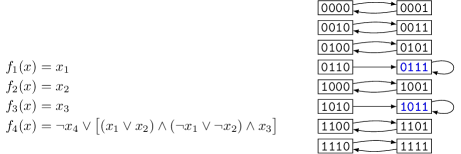
Figure 1: Example deterministic Boolean automata network of size $n=4$. Local functions $f_{i}:\{0,1\}^{4}\to\{0,1\}$ for $i\in[n]$ (left) and transition digraph dynamics $\mathcal{G}_{f}$ on configuration space $\{0,1\}^{4}$ (right).

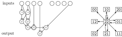
Figure 2: Example non-deterministic $q$-uniform automata network of size $n=2$ on alphabet $\llbracket q\rrbracket=\{0,1,2\}$ with $q=3$. Circuit of the relation $f\subseteq\llbracket q\rrbracket^{n}\times\llbracket q\rrbracket^{n}$ (left) and transition digraph dynamics $\mathcal{G}_{f}$ on configuration space $\llbracket q\rrbracket^{n}$ (right). A configuration is encoded on four bits, where inputs $0000$ to $0001$ correspond respectively to configurations $00$ to $22$. The doubly circled node represents the evaluation of propositionnal formula $S=(x_{1}\vee x_{2})\wedge(\neg x_{1}\vee\neg x_{2})\wedge x_{3}$ on the three first bits of the circuit’s input.

Remark 1.

For all graph $G$, there exists a NAN $f$ such that $\mathcal{G}_{f}=G$ (up to a renaming of the vertices). If $G$ has out-degree $1$, then there is also such an AN $f$. In particular, we can set $n=1$ automaton with state set $A_{1}=V(G)$. It also holds for $q$-uniform networks, provided the graph $G$ has size $q^{n}$ for some integer $n$.

Given our focus on computational complexity, it is important to explicit how ANs and NANs are encoded, to be given as inputs to problems. An AN $f$ is encoded as one Boolean circuit with $\lceil\log_{2}|X|\rceil$ input bits and $\lceil\log_{2}|X|\rceil$ output bits. The state set sizes $(|A_{i}|)_{i\in[n]}$ are also part of the input, to encode/decode configurations as bitstrings. Given a configuration $x\in X$ as input to the circuit, its image $f(x)$ is read as the output taken modulo $|X|$ (to avoid the ${\mathsf{coNP}}$-complete problem of checking that the circuit always outputs a bitstring from $0$ to $|X|-1$). In the Boolean case, each input/output bit of the circuit is the state of an automaton (circuits generalize propositional formulas, but all our results still hold for an encoding through formulas). A NAN $f$ is encoded as one Boolean circuit with $2\cdot\lceil\log_{2}|X|\rceil$ input bits and $1$ output bits, indicating whether the two input configurations $x$ and $y$ verify $y\in f(x)$. The circuit size of an AN is restricted to some $\mathcal{O}(|X|\log_{2}|X|)$ (the size of a lookup table for $\mathcal{G}_{f}$ of out-degree $1$), and that of a NAN to some $\mathcal{O}(|X|^{2})$ (the size of an adjacency matrix for $\mathcal{G}_{f}$). These encodings are also called succinct graph representations of $\mathcal{G}_{f}$. When constructing ANs or NANs in our proofs, it will always be straightforward to convert (in polynomial time) our descriptions of dynamics into local functions and their encodings as circuits. Examples of AN and NAN are given on Figures 1 and 2, respectively.

2.2 Graph Logics

If $P$ is a property that automata networks may or may not satisfy, and $f$ is an AN or a NAN, then we write $f\vDash P$ if $f$ satisfies $P$, and $f\nvDash P$ otherwise. We say that $f$ is a model of $P$ in the first case, and a counter-model otherwise. This is an abuse of notation, and we need to know the exact nature of $P$ to know its precise meaning. In particular, we will study properties expressible on Graph Monadic Second Order Logic (MSO) over the signature $\{=,\to\}$, where $\to$ is a binary relation such that $x\to y$ if and only if $y=f(x)$ or $y\in f(x)$ (that is, $(x,y)\in E(\mathcal{G}_{f})$). Our formulas express graphical properties of $\mathcal{G}_{f}$, with logical operators ($\wedge$, $\vee$, $\neg$, $\implies$), and quantifications ($\exists,\forall$) on vertices (configurations) or sets of vertices (with the adjonction of $\in$ to the signature, for set membership). The quantifier rank of a formula $\psi$ is its depth of quantifier nesting, see for example [19, Definition 3.8]. If $G$ and $G^{\prime}$ are two structures, we write $G\equiv_{m}G^{\prime}$ when they satisfy the same formulas of quantifier rank $m$. We write $\psi\equiv\psi^{\prime}$ when the two formulae $\psi$ and $\psi^{\prime}$ have the same models and the same counter-models.

We will express general complexity lower bounds for non-trivial fromulas, but this notion depends on the ANs or NANs under consideration. A formula $\psi$ is non-trivial when it has infinitely many models and infinitely many counter-models, among graphs of out-degree $1$. A formula $\psi$ is arborescent when there exists $k$ such that $\psi$ has infinitely many models of treewidth at most $k$ and infinitely many counter-models of treewidth at most $k$ (the definition of treewidth is recalled below). According to Remark 1, these notions respectively correspond to deterministic ($\mathcal{G}_{f}$ for ANs) and non-deterministic ($\mathcal{G}_{f}$ for NANs) dynamics. When considering only graphs $\mathcal{G}_{f}$ for $q$-uniform networks, we obtain the notions of $q$-non-trivial and $q$-arborescent formulas.

In this article, the dynamical complexity of ANs and NANs is studied through an algorithmic point of view and the following families of decision problems, aimed at asking general properties on the behavior of a given network (the MSO formula $\psi$ is fixed in the problem definition).

$\psi$-AN-dynamics
Input: circuit of an AN $f$ of size $n$. Question: does $\mathcal{G}_{f}\vDash\psi$? $\psi$-$q$-AN-dynamics
Input: circuit of a $q$-AN $f$ of size $n$. Question: does $\mathcal{G}_{f}\vDash\psi$?

$\psi$-NAN-dynamics
Input: circuit of an NAN $f$ of size $n$. Question: does $\mathcal{G}_{f}\vDash\psi$? $\psi$-$q$-NAN-dynamics
Input: circuit of a $q$-NAN $f$ of size $n$. Question: does $\mathcal{G}_{f}\vDash\psi$?

Example formulas and associated $\psi$-AN-dynamics problems:

• $\exists x,x\to x$ means that $f$ has a fixed point,

• $\exists x,\forall y,y\to x$ means that $f$ is a constant,

• $\forall x,\exists y,x\to y$ is trivially true,

• $\forall x,\forall y,\forall x^{\prime},\forall y^{\prime},(x\to y\wedge x^{\prime}\to y^{\prime}\wedge y=y^{\prime})\implies x=x^{\prime}$ means that $f$ is injective,

• $\exists x,x\to x\wedge(\forall y,y\neq x\implies(\exists z,y\neq z\wedge y\to z\wedge z\to y))$ requires $|V(\mathcal{G}_{f})|$ to be odd, hence it is non-trivial in general, but trivial in the Boolean case.

For $\psi$-NAN-dynamics (non-deterministic) we have the following examples:

• $\exists X,(\exists x\in X)\wedge(\forall x\in X,\exists y\in X:x\neq y\wedge x\to y)$ means that $\mathcal{G}_{f}$ has at least one non-trivial strongly connected component,

• $\forall x,\exists y,x\to y\wedge(\forall z,z\neq y\implies\neg(x\to z))$ means that $\mathcal{G}_{f}$ has out-degree $1$, which is trivial on determistic dynamics.

Most formulas above do not use the second order quantifier, hence they are First Order (FO) formulas. It is known that properties such as connecitivity, acyclicity, 2-colorability and planarity are expressible in MSO, but not in FO [19, Chapter 3].

Observe that the signature $\{=,\to\}$ only allows to express properties up to isomorphism, that is if $\mathcal{G}_{f}$ and $\mathcal{G}_{g}$ are isomorphic then $\mathcal{G}_{f}\equiv_{m}\mathcal{G}_{g}$ for all $m$.

If $\psi$ is trivial (resp. $q$-trivial), then $\psi$-AN-dynamics (resp. $\psi$-$q$-AN-dynamics) has a finite list of positive instances or a finite list of negative instances, hence it is solvable in constant time.

2.3 Boundaried graphs and equivalence classes

Let $k\in\mathbb{N}$. A $k$-boundaried graph is a digraph $G$ equipped with a sequence $P(G)=(p_{1},...,p_{k})$ of $k$ distinct vertices from $V(G)$, called ports. Given two $k$-boundaried graphs $G$, $G^{\prime}$ with ports $P(G)=(p_{1},...,p_{k})$ and $P(G^{\prime})=(p^{\prime}_{1},...,p^{\prime}_{k})$, we define their gluing as $G\oplus G^{\prime}=H$ with:

$$V(H) =V(G)\cup(V(G^{\prime})\backslash P(G^{\prime})),$$

$$E(H) =E(G)\cup E(G^{\prime}[P(G)\leftarrow P(G^{\prime})]),$$

$$P(H) =P(G),$$

where $G^{\prime}[P(G)\leftarrow P(G^{\prime})]$ denotes the graph $G^{\prime}$ where port $p^{\prime}_{i}$ is renamed $p_{i}$ (for $i\in[k]$). In words, we take the union of $G$ and $G^{\prime}$, then merge port $p_{i}$ of $G$ with port $p^{\prime}_{i}$ of $G^{\prime}$, while keeping all the edges. Observe that $\oplus$ is, strickly speaking, not commutative in general (because we keep the port vertices from the left graph, although $G\oplus G^{\prime}$ is isomorphic to $G^{\prime}\sqcup G$), but for $k=0$ we have $G\oplus G^{\prime}=G\sqcup G^{\prime}$.

A $k$-biboundaried graph is a digraph $G$ equipped with two sequences of $k$ ports: the primary ports $P_{1}(G)$, and the secondary ports $P_{2}(G)$. We still have $P_{i}(G)\subseteq V(G)$ for $i\in\{1,2\}$, but we do not necessarily have $P_{1}(G)\cap P_{2}(G)=\emptyset$. Given two $k$-biboundaried graphs $G$, $G^{\prime}$, considering them as $k$-boundaried with $P(G)=P_{2}(G)$ and $P(G^{\prime})=P_{1}(G^{\prime})$, and denoting $H=G\oplus G^{\prime}$ (for the $k$-boundaried graphs), we define the gluing of the two $k$-biboundaried graphs as $G\oplus G^{\prime}=H^{\prime}$ with

$$V(H^{\prime}) =V(H),$$

$$E(H^{\prime}) =E(H),$$

$$P_{1}(H^{\prime}) =P_{1}(G),$$

$$P_{2}(H^{\prime}) =P_{2}(G^{\prime}).$$

In words, we take the union of $G$ and $G^{\prime}$, then merge ports $P_{2}(G)$ with $P_{1}(G^{\prime})$. The operation $\oplus$ is not commutative in general, although it still corresponds to the disjoint union for $k=0$.

As the reader can observe, we overload $\oplus$ and it becomes unclear whether it applies to boundaried or biboundaried graphs. To prevent ambiguities, we consider a boundaried graph $G$ as biboundaried with $P_{1}(G)=P_{2}(G)=P(G)$ (this conversion commutes with $\oplus$). A $k$-biboundaried graph is called a $k$-graph, for short. The operator $\oplus$ only applies to graphs with the same number $k$ of ports. Primary (resp. secondary) ports are not necessary to obtain a digraph from right (resp. left) gluing, therefore we will sometimes omit them. See Figure 3 for an example.

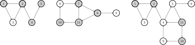
Figure 3: Example biboundaried graphs and their gluing. Primary ports are represented by hatched nodes, and secondary ports by grey nodes. A graph $G$ with $P_{1}(G)=(1,3)$ and $P_{2}(G)=(4,5)$ (left). A graph $G^{\prime}$ with $P_{1}(G^{\prime})=(7,6)$ and $P_{2}(G^{\prime})=(10,11)$ (middle). The graph $G\oplus G^{\prime}=H$ with $P_{1}(H)=(1,3)$ and $P_{2}(H)=(10,11)$ (right).

Now let $\Gamma=\{G_{i}\}_{i\in\mathcal{I}}$ be a finite family of $k$-graphs. For $\omega=\omega_{1}\dots\omega_{\mu}$ a nonempty word over alphabet $\mathcal{I}$, the operation $\Delta^{\Gamma}(\omega)$ is defined by induction on the length $\mu\in\mathbb{N}_{+}$ of $\omega$ as follows:

$$\Delta^{\Gamma}(\omega_{1})=G_{\omega_{1}},\qquad\Delta^{\Gamma}(\omega_{1}\dots\omega_{\mu})=\Delta^{\Gamma}(\omega_{1}\dots\omega_{\mu-1})\oplus G_{\omega_{\mu}}.$$

Let $G,G^{\prime}$ be $k$-graphs. Given an MSO sentence $\psi$, we write $G\sim_{k,\psi}G^{\prime}$ if and only if for every $k$-graph $H$, we have: $G\oplus H\vDash\psi\iff G^{\prime}\oplus H\vDash\psi$.

Denote $\Sigma_{k,\psi}$ the set of equivalence classes of $\sim_{k,\psi}$ for $k$-graphs. By [5, Theorem 13.1.1], if $k$ and $\psi$ are fixed then $\Sigma_{k,\psi}$ is finite.

We may drop subscripts $k$ and/or $\psi$ when they are clear from the context.

2.4 Tree-decompositions and treewidth

All our graphs will be directed. The subtree of a tree $T$ rooted in vertex $v\in V(T)$ is the induced subgraph obtained from the descendants of $v$ (the root of the subtree).

A tree-decomposition of a digraph $G=(V,E)$ is a tree $T$ whose nodes are labelled with ordered (to become ports) subsets of $V$, called bags, satisfying the three conditions below. If $v$ is a node of $T$, we write $B_{T}(v)\subseteq V$ the corresponding bag (when $T$ is clear from the context, we drop the subscript notation).

1. Every vertex $x$ of $G$ is containted in at least one bag $B(v)$ of $T$.

2. For every edge $(x,y)$ of $G$, both vertices $x$ and $y$ are contained in at least one bag $B(v)$ of $T$.

3. For each vertex $x$ of $G$, the subgraph $T^{\prime}$ of $T$ restricted to vertices whose bag contains $x$ is connected.

A graph may admit multiple tree-decompositions. The width of a tree-decomposition $T$ is the size of its largest bag minus one, ie. $w(T)=\max\{|B(t)|\mid t\in V(T)\}-1$. The treewidth of a graph $G$, written $tw(G)$, is the minimal width among all of its tree-decompositions. A tree-decomposition $T$ of width $w(T)=k$ is called a $k$-tree-decomposition, and we assume without loss that all bags of $T$ are of size $k+1$. For the corresponding graph $G$, it means that $tw(G)\leq k$. Remark that a functional digraph can be very similar to its tree-decomposition.

Given a graph $G$, a tree-decomposition $T$ and an MSO formula $\psi$, for each $v\in V(T)$ we denote:

• $\mathcal{S}_{T}(v)$ the largest subtree of $T$ rooted in $v$,

• $\mathcal{N}_{T}(v)$ the boundaried graph resulting from the subgraph of $G$ spanned by the vertices appearing in bags of $\mathcal{S}_{T}(v)$, ie. $\bigcup_{u\in V(\mathcal{S}_{T}(v))}B(u)$, with ports $B(v)$,

• $\mathcal{C}_{T}(v)$ is the equivalence class of $\mathcal{N}_{T}(v)$ for the relation $\sim_{\psi}$.

See Figure 4 for an example.

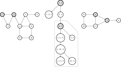
Figure 4: A graph $H$ (left) and its tree-decomposition $T$ (middle). In the tree-decomposition a node $v$ such that $B(v)=(4,5)$ is highlighted, with the subtree $\mathcal{S}_{T}(v)$ surrounded with a dashed line. The graph $\mathcal{N}_{T}(v)$ (right) where the primary ports, from the root bag of $\mathcal{S}_{T}(v)$, are hatched.

When the tree $T$ is clear from the context, we drop the subscript notation. Two nodes $v,v^{\prime}\in V(T)$ are said to be $\mathcal{N}$-different, written $v\neq v^{\prime}$, when $\mathcal{N}(v)\neq\mathcal{N}(v^{\prime})$. The $\mathcal{N}$-size of $T$ is its number of $\mathcal{N}$-different nodes (hence at most $2^{|G|}$, because the order of vertices inside the bags does not matter). The $\mathcal{N}$-length of a path $\mathcal{P}$ in $T$ is the number of $\mathcal{N}$-different nodes it goes through.

When gluing two $k$-tree-decompositions $T\oplus T^{\prime}$, ports will be single vertices (in the trees, $P_{1}(T^{\prime})$ will be the root of $T^{\prime}$ and $P_{2}(T)$ will be a leaf of $T$) and we merge their bags (of size $k+1$) by renaming all the bags of $T^{\prime}$ according to the substitution $B(P_{1}(T^{\prime}))\leftarrow B(P_{2}(T))$. Formally, we define $T\oplus T^{\prime}=T^{\prime\prime}$ in terms of $1$-graphs, and set the following bags for $T^{\prime\prime}$:

• For all $v\in V(T)$, set $B_{T^{\prime\prime}}(v)=B_{T}(v)$,

• For all $v\in V(T^{\prime})\setminus P_{1}(T^{\prime})$, set $B_{T^{\prime\prime}}(v)=B_{T^{\prime}}(v)[B(P_{1}(T^{\prime}))\leftarrow B(P_{2}(T))]$.

In words, we merge the bags of the merged vertices, and propagate this substitution to all the other bags of $T^{\prime}$. See Figure 5 for an example.

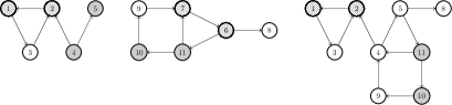
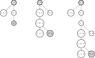
Figure 5: Graphs $G$, $G^{\prime}$ and $G\oplus G^{\prime}$ from Figure 3, with their respective tree-decompositions below. In the trees, primary ports are represented by hatched bags, and secondary ports by grey bags. Let $T$ (left) and $T^{\prime}$ (middle) be the respective tree-decompositions of $G$ and $G^{\prime}$, then $T\oplus T^{\prime}$ (right) is a tree-decomposition of $G\oplus G^{\prime}$. Notice the propagation of the renaming of vertices from the merged bags: $(7,6)\leftarrow(4,5)$.

As $\Delta^{\Gamma}(\omega)$ for graphs, we define a similar operation for $k$-tree-decompositions. Let $\mathcal{T}=\{T_{i}\}_{i\in\mathcal{I}}$ be a finite family of $k$-tree-decompositions, each with their root as primary port, and a leaf as secondary port. For $\omega=\omega_{1}...\omega_{\mu}$ a nonempty word over alphabet $\mathcal{I}$, the operation $\Lambda^{\mathcal{T}}$ is defined by induction on $\mu$ as:

$$\Lambda^{\mathcal{T}}(\omega_{1})=T_{\omega_{1}},\qquad\Lambda^{\mathcal{T}}(\omega_{1}...\omega_{\mu})=\Lambda^{\mathcal{T}}(\omega_{1}...\omega_{\mu-1})\oplus T_{\omega_{\mu}}.$$

Given a formula $\psi$, a $k$-tree-decomposition of $G$ can be viewed as a $\Sigma_{k+1}$-labeled tree, by labeling each node $v$ with $\mathcal{C}(v)$ instead of the bag $B(v)$. This is especially useful thanks to the following remark.

Remark 2 ([10, Remark 15]).

Let $\Gamma=\{G_{i}\}_{i\in\mathcal{I}}$ be a family of $k$-graphs and $\mathcal{T}=\{T_{i}\}_{i\in\mathcal{I}}$ be a family of $\Sigma_{k}$-labeled trees, both indexed by the same finite set $\mathcal{I}$. Suppose that for every $i$, the tree $T_{i}$ corresponds to a decomposition of $G_{i}$ such that:

• the primary port of $T_{i}$ is its root $r$, and $B(r)=P_{1}(G_{i})$,

• the secondary port of $T_{i}$ is a leaf $\ell$, and $B(\ell)=P_{2}(G_{i})$.

Then, for every nonempty word $\omega$ over alphabet $I$, the tree $\Lambda^{\mathcal{T}}(\omega)$ corresponds to a decomposition of $\Delta^{\Gamma}(\omega)$.

For a formula $\psi$, we say that a $\Sigma$-labeled tree is positive when it corresponds to a model of $\psi$ (and negative otherwise). A $\Sigma$-labeled tree can correspond to several different graphs, but from Remark 2 they are all models, or they are all counter-models.

3 Previous works

The computational complexity of questions on the dynamics of automata networks has traditionally raised a great interest, as a mean to understand the possibilities and limits of algorithmic problem solving, in this model and multiple variants with restrictions on the type of local functions (e.g. Boolean, theshold, disjunctive), the architecture of the network, or with different update modes. Alon noticed in [1] that it is ${\mathsf{NP}}$-hard to decide whether a given BAN has a fixed point. Floréen and Orponen then settled the complexity of multiple problems related to fixed points [7, 27]. Further developments [17] include the study of limit cycles [3, 31], update modes [28, 26, 3, 2] and specific rules [12, 11, 13].

In a recent series of two papers [9, 10], Rice-like complexity lower bounds have been established, encompassing at once many results from the literature. They state that non-trivial formulas yield algorithmically hard $\psi$-dynamics problems. The first article concentrates on the deterministic setting and FO formulas (using Hanf-Gaifman’s locality), while the second article brings the result to MSO on non-deterministic automata networks (and introduces the notion of arborescent formula).

Theorem 1.a for FO ([9, Theorem 5.2]).

For any non-trivial FO formula $\psi$, problem $\psi$-AN-dynamics is ${\mathsf{NP}}$-hard or ${\mathsf{coNP}}$-hard.

Theorem 1.c ([10, Theorem 1]).

For any arborescent MSO formula $\psi$, problem $\psi$-NAN-dynamics is ${\mathsf{NP}}$-hard or ${\mathsf{coNP}}$-hard.

In the present work, we bring these results to $q$-uniform ANs and NANs, for MSO formulas (Theorem 1). Indeed, the reductions presented in the proofs of [9, Proposition 5.1.2 and Lemma 5.1.4] and [10, Proposition 19 and Lemma 20] may require arbitrary alphabet sizes in the construction of instances of $\psi$-AN-dynamics and $\psi$-NAN-dynamics, respectively. The proof of Theorem 1 is based on the abstract pumping technique introduced in [9] and developed in [10], which is reviewed in the rest of this section.

Let us start with the example of Figure 1. It implements a reduction from SAT (here with $S=[(x_{1}\vee x_{2})\wedge(\neg x_{1}\vee\neg x_{2})\wedge x_{3}]$ on 3 Boolean variables), to prove the ${\mathsf{NP}}$-hardness of the fixed point existence problem ($\exists x:x\to x$). Indeed, for each valuation $v\in\{0,1\}^{3}$ of $S$, the pair of configurations $x,x^{\prime}\in\{0,1\}^{4}$ with $x_{\{1,2,3\}}=x^{\prime}_{\{1,2,3\}}=v$ creates either:

• a path with a loop when $v\models S$, or

• a cycle of length $2$ when $v\not\models S$.

Observe that this same reduction also proves the ${\mathsf{coNP}}$-hardness of asking whether the dynamics is a union of limit cycles of length $2$, and of asking whether the dynamisc is injective, both by reduction from UNSAT. The basic idea to reduce from SAT or UNSAT is to evaluate $S$ on the configuration, and produce (glue) one of two graphs $G_{0},G_{1}$ (using a distinct subset of configurations for each valuation) according to whether the formula is satisfied or not. If the formula is satisfiable then $G_{0}$ appears at least once, otherwise there are only copies of $G_{1}$. The crucial part is then to obtain appropriate graphs $G_{0}$ and $G_{1}$ for any non-trivial (or arborescent) MSO formula $\psi$, and this requires tools from finite model theory (giving additional parts $G_{2},G_{3}$ to deal with). Analogously, the example of Figure 2 is strongly connected if and only if $S$ is a tautology.

Remark that $\psi$ is fixed in the problem definition, therefore $G_{0},G_{1}$ are considered constant. Also, reductions produce circuits for the local functions, not the transition digraph itself. From [10] we first introduce the concept of saturating graph $G_{0}$ (Subsection 3.1), then the requirement on $G_{1}$ to produce a metareduction (Subsection 3.2), and finaly how $G_{1}$ has been obtained via the abstract pumping technique (Subsection 3.3). We close this section with an overview of our contributions on strengthening this proof scheme (Subsection 3.4).

3.1 Saturating graph

In [10] it is shown that for all $m\in\mathbb{N}$, there exists a saturating graph $\Omega_{m}$ such that, for all MSO formulas $\psi$ of rank $m$, if a graph contains a copy of $\Omega_{m}$ then it is forced to be a model of $\psi$ (if $\Omega_{m}$ is a sufficient subgraph for $\psi$) or a counter-model of $\psi$ (if $\Omega_{m}$ is a forbidden subgraph for $\psi$).

Proposition 2 ([10, Proposition 5]).

Fix $m\in\mathbb{N}$. There exists a graph $\Omega_{m}$ such that, for every MSO formula $\psi$ of rank $m$, either:

1. for every graph $G$ we have $G\sqcup\Omega_{m}\vDash\psi$, or

2. for every graph $G$ we have $G\sqcup\Omega_{m}\nvDash\psi$.

The proof consists in considering $\Omega_{m}$ to be the disjoint union of sufficiently many copies of representatives from all equivalence classes of $\equiv_{m}$, so that $m$-round Ehrenfeucht–Fraïssé games cannot distinguish any additional copy ($G$ in the statement). It is immediate that the same proof applies when considering only graphs of out-degree $1$, because disjoint union preserves this property.

Corollary 3.

Fix $m\in\mathbb{N}$. There exists a graph $\Omega_{m}$ of out-degree $1$ such that, for every MSO formula $\psi$ of rank $m$, either:

1. for every graph $G$ of out-degree $1$ we have $G\sqcup\Omega_{m}\vDash\psi$, or

2. for every graph $G$ of out-degree $1$ we have $G\sqcup\Omega_{m}\nvDash\psi$.

It will be clear from the context which of the two $\Omega_{m}$ we are considering: Proposition 2 for non-deterministic dynamics, and Corallary 3 for deterministic dynamics.

3.2 Metareduction

For a given MSO formula $\psi$ of rank $m$, whether $\Omega_{m}$ is sufficient (a model of $\psi$) or forbidden (a counter-model of $\psi$) indicates whether we respectively reduce from SAT (${\mathsf{NP}}$-hardness) or UNSAT (${\mathsf{coNP}}$-hardness). Given a propositional formula $S$ on $s$ variables, the configuration space $X$ is partitioned into $2^{\ell}$ subsets of configurations, so that $S$ is evaluated on each subset:

• if $S$ is satisfied then those vertices create a copy of $\Omega_{m}$,

• if $S$ is falsified then those vertices create a neutral graph.

The neutral is intending to “change nothing”, and is obtained by pumping (see next Subsection). However, tools from finite model theory provide four graphs, meeting the requirements stated below.

Proposition 4 ([10, Proposition 19]).

Let $\psi$ be an MSO formula and $\Gamma=\{G_{0},G_{1},G_{2},G_{3}\}$ four $k$-graphs for some $k\in\mathbb{N}$, such that:

1. $|G_{0}|=|G_{1}|$,

2. $P_{1}(G_{0})\cap P_{2}(G_{0})=P_{1}(G_{1})\cap P_{2}(G_{1})\neq V(G_{1})$, and

3. for every $p$ in $P_{1}(G_{0})\cap P_{2}(G_{0})$, we have $G_{0}(p)=G_{1}(p)$.

Suppose that, for every word $w$ over alphabet $\{0,1\}$, we have $\Delta^{\Gamma}(2\cdot w\cdot 3)\vDash\psi$ if and only if $w$ contains letter $0$. Then $\psi$-NAN-dynamics is ${\mathsf{NP}}$-hard.

To prove the proposition, it requires to take into account vertices merged by the gluing operations, in order to construct a NAN $f$ of appropriate size, so that each configuration (vertex of $\mathcal{G}_{f}$) plays its expected role. We denote $\overline{S}$ the word of length $2^{s}$ on alphabet $\{0,1\}$ such that $\overline{S}_{i}$ is $1$ when the assignment $i$ satisfies $S$, and is $0$ otherwise ($i$ being interpreted as a $s$ bits assignment). The reduction builds the circuit of a NAN whose dynamics is $\Delta^{\Gamma}(2\cdot\bar{S}\cdot 3)$. The only non-constant part of the construction consists in evaluating $S$.

3.3 Pumping models and counter-models

Let us sketch how the four graphs from Proposition 4 are obtained. In particular the neutral element, in the next proposition.

Proposition 5 ([10, Proposition 8]).

Let $\psi$ be an MSO formula and an integer $k$. If $\psi$ has infinitely many models of treewidth $k$, then there exist $\tilde{\Gamma}=\{\tilde{G_{1}},\tilde{G_{2}},\tilde{G_{3}}\}$ three $(k+1)$-graphs such that $\Delta^{\tilde{\Gamma}}(2\cdot 1^{\ell}\cdot 3)\vDash\psi$ for all $\ell\in\mathbb{N}$, and $P_{1}(\tilde{G_{1}})\cap P_{2}(\tilde{G_{1}})\neq V(G_{1})$.

The proof relies on Remark 2. Since $\Sigma_{k}$ is finite, considering a sufficiently big model ensures that there exists a part that can be pumped, denoted $\tilde{G_{1}}$. It is identified on tree-decompositions, and glued in terms of graphs thanks to Remark 2.

In order to furhtermore obtain Conditions 1–3 of Proposition 4, the graph $\Omega_{m}$ will play the role of $G_{0}$. If $\Omega_{m}$ is a counter-model of $\psi$, then we consider $\neg\psi$ instead of $\psi$ (so that $\Omega_{m}$ is sufficient; and Proposition 5 is applied on $\neg\psi$). Observe that $\Omega_{m}$ can accomodate any disjoint union yet remain saturating. Take $G_{0}$ as the disjoint union of $\Omega_{m}$ and $\tilde{G_{1}}$. On the other side, take $G_{1}=\bigoplus_{i=1}^{\alpha}\tilde{G_{1}}$ with $\alpha$ such that $|G_{1}|\geq|G_{0}|$. Finaly, pad $G_{0}$ in order to have $|G_{0}|=|G_{1}|$. Then with $G_{2}=\tilde{G_{2}}$ and $G_{3}=\tilde{G_{3}}$ we indeed obtain all the resquirements for Proposition 4.

To conclude the hardness proof by reduction from SAT or UNSAT, it remains to construct the circuit of an automata network such that the dynamics has: one copy of $G_{2}$, then copies of $G_{0}$ or $G_{1}$ for the $2^{\ell}$ subsets of configurations on which the formula $S$ is evaluated, and finaly one copy of $G_{3}$. All these copies also need to be glued correctly by the circuit, which is easy to process in polynomial time.

3.4 Contributions

To prove Theorem 1, our contributions in this paper will be twofold.

• A careful consideration in gluing deterministic dynamics (graphs of out-degree $1$ are handled through Hanf’s local lemma in [9]) in Section 4.

• The adjunction of arithmetical considerations in Section 5, to restrict the constructions to $q$-uniform networks in Section 6.

4 Complexity lower bounds for deterministic networks

In this section, we extend Theorem 1.a for FO from FO to MSO logics, or more accurately we transpose the proof technique of Theorem 1.c from non-deterministic to deterministic dynamics, which are succinctly represented graphs of out-degree $1$. Recall that the non-triviality of formulas is defined relative to graphs of out-degree $1$ only. We prove the following part of Theorem 1.

Theorem 1.a.

For any non-trivial MSO formula $\psi$, problem $\psi$-AN-dynamics is ${\mathsf{NP}}$-hard or ${\mathsf{coNP}}$-hard.

We follow the proof structure presented in Section 3, using the deterministic saturating graph from Corollary 3. The main difficulty consists in transposing Proposition 5 in order to obtain graphs of out-degree $1$ all along the way (i.e., to ensure that gluings preserve this property), and meet Conditions 1–3 of Proposition 4. We combine these into the following proposition (out-degree $1$ graphs have treewidth at most $2$).

Proposition 6.

Let $\psi$ be an MSO formula. If $\psi$ has infinitely many models of out-degree $1$, then there exist $\tilde{\Gamma}=\{\tilde{G}_{1},\tilde{G}_{2},\tilde{G}_{3}\}$ three $3$-graphs such that $\Delta^{\tilde{\Gamma}}(2\cdot 1^{\ell}\cdot 3)\models\psi$ for all $\ell\in\mathbb{N}$, and $P_{1}(\tilde{G_{1}})\cap P_{2}(\tilde{G_{1}})\neq V(\tilde{G_{1}})$. Moreover, $\Delta^{\tilde{\Gamma}}(2\cdot 1^{\ell}\cdot 3)$ has out-degree $1$ for all $\ell\in\mathbb{N}$.

Our trick to prove Proposition 6 consists in introducing the property of having out-degree $1$ as an MSO formula. Let:

$$\chi=\forall x,\exists y,(x\to y)\wedge(\forall z,z\neq y\implies\neg(x\to z)),$$

such that $G\vDash\chi$ if and only if the graph $G$ has out-degree exactly $1$ (is a deterministic dynamics, or a functional graph).

Recall that $\Sigma_{k,\psi}$ denotes the set of equivalence classes of $\sim_{k,\psi}$ for $k$-graphs. It is finite for any given $k$ and $\psi$, hence $\Sigma_{k,\psi,\chi}=\Sigma_{k,\psi}\times\Sigma_{k,\chi}$ is finite as well. In the rest of this section $k=3$, so we drop it from the notation. When considering $\Sigma_{\psi,\chi}$-labeled trees, each node $v$ has an assocatied equivalence classe $\mathcal{C}(v)$, and we also define $\mathcal{C}^{\psi}(v)$ and $\mathcal{C}^{\chi}(v)$ for the equivalences classes for $\psi$ and $\chi$, respectively. Hence, for two nodes $v$ and $v^{\prime}$ of a $\Sigma_{\psi,\chi}$-labeled tree, we have $\mathcal{C}(v)=\mathcal{C}(v^{\prime})$ if and only if $\mathcal{C}^{\psi}(v)=\mathcal{C}^{\psi}(v^{\prime})$ and $\mathcal{C}^{\chi}(v)=\mathcal{C}^{\chi}(v^{\prime})$. We are now able to prove the proposition.

Proof.

This proof brings the ideas of [10] to the deterministic setting. Since $\psi$ has infinitely many deterministic models, we consider a family $(M_{i})_{i\in\mathbb{N}}$ of deterministic models and $(D_{i})_{i\in\mathbb{N}}$ a sequence of their $3$-tree-decompositions, such that each $D_{i}$ has at least one path of $\mathcal{N}$-length $i$ (which is possible by splitting nodes of degree more than three in the tree). Without loss of generality we assume that every $M_{i}$ has at least $3$ vertices, and that all the bags of $D_{i}$ are of size $3$.

We view the tree-decompositions $D_{i}$ as $\Sigma_{\psi,\chi}$-labeled trees. Let $s=|\Sigma_{\psi,\chi}|$. Any path of $\mathcal{N}$-length at least $s+1$ in a tree-decomposition contains two $\mathcal{N}$-different nodes with the same label. In particular, $D_{s+1}$ contains a path with two $\mathcal{N}$-different vertices $v$ and $v^{\prime}$, such that $\mathcal{C}(v)=\mathcal{C}(v^{\prime})$. Assume that $v$ is higher than $v^{\prime}$ in the tree, and recall that $\mathcal{S}(v)$ is the largest subtree of $D_{s+1}$ rooted in $v$. We define:

$$T_{1}=(\mathcal{S}(v)\backslash\mathcal{S}(v^{\prime}))\cup\{v^{\prime}\},\qquad T_{2}=(D_{s+1}\backslash\mathcal{S}(v))\cup\{v\},\qquad T_{3}=\mathcal{S}(v^{\prime}),$$

so that we have $T_{2}\oplus T_{1}\oplus T_{3}=D_{s+1}$ (choosing the bags of $v$ and $v^{\prime}$ as ports). Since $\mathcal{C}(v)=\mathcal{C}(v^{\prime})$, and in particular $\mathcal{C}^{\psi}(v)=\mathcal{C}^{\psi}(v^{\prime})$, by [10, Lemma 14] we deduce that $\Lambda^{\mathcal{T}}(2\cdot 1^{\ell}\cdot 3)$ is positive for $\psi$ for all $\ell\in\mathbb{N}$. Then, by Remark 2, there exist $\tilde{\Gamma}=\{\tilde{G}_{1},\tilde{G}_{2},\tilde{G}_{3}\}$ associated respectively to $T_{1},T_{2},T_{3}$ such that $\Delta^{\tilde{\Gamma}}(2\cdot 1^{\ell}\cdot 3)$ is a model of $\psi$ for all $\ell\in\mathbb{N}$ (remark that by definition of $\mathcal{N}$-difference, there exists at least one vertex in $G_{1}$ which is not both a primary port nor a secondary port, that is $P_{1}(\tilde{G_{1}})\cap P_{2}(\tilde{G_{1}})\neq V(G_{1})$, hence the sequence $(|\Delta^{\Gamma}(2\cdot 1^{\ell}\cdot 3)|)_{\ell\in\mathbb{N}}$ is strictly increasing). Analogously, we deduce that $\Delta^{\Gamma}(2\cdot 1^{\ell}\cdot 3)$ is a model of $\chi$ for all $\ell\in\mathbb{N}$, hence that all these graphs have out-degree $1$. ∎

Let $\Omega_{m}$ denote the deterministic saturating graph from Corollary 3, employed to reach Conditions 1–3 of Proposition 4, and the positivity if and only if the $\Delta^{\Gamma}$ gluing contains at least one copy of $G_{0}$.

Proof of Theorem 1.a.

Let $\tilde{\Gamma}=\{\tilde{G}_{1},\tilde{G}_{2},\tilde{G}_{3}\}$ be given by Proposition 6. Consider $\tilde{G_{0}}=\Omega_{m}\sqcup\tilde{G_{1}}$, such that Conditions 2–3 of Proposition 4 (relative to the ports) are verified, and $\tilde{G_{0}}$ is still deterministic. Now, let $G_{1}=\bigoplus_{i=1}^{n}\tilde{G_{1}}$ with $n$ such that $|G_{1}|\geq|\tilde{G_{0}}|$, and let $G_{0}$ be $\tilde{G_{0}}$ with $|G_{1}|-|\tilde{G_{0}}|$ additionnal isolated fixed points. We have $|G_{0}|=|G_{1}|$ (Condition 1), and the proof is completed by taking $G_{2}=\tilde{G}_{2}$ and $G_{3}=\tilde{G}_{3}$. Indeed, thanks to the deterministic saturating graph $\Omega_{m}$ from Corollary 3, it holds that $\Delta^{\Gamma}(2\cdot w\cdot 3)$ is a model of $\psi$ if and only if $w\in\{0,1\}^{*}$ contains at least one letter $0$.

It is now straightforward to build a polytime metareduction from $\Gamma=\{G_{0},G_{1},G_{2},G_{3}\}$, as in Proposition 4 from [10] (see Section 3.2). An out-degree $1$ graph on $N$ vertices is encoded as a circuit with $\log_{2}(N)$ input bits and $\log_{2}(N)$ output bits. ∎

5 Arithmetics for uniform networks

In this section we study the intersection of pairs of number sequences, to the purpose of constructing a metareduction proving Theorem 1 for $q$-uniform automata networks (with a fixed alphabet of size $q$). We start by considering the restriction to Boolean alphabets, which is simpler. In Subsection 5.1, we extract regularities in the intersection of the two sets of integers $\{ak+b\mid k\in\mathbb{N}_{+}\}$ and $\{2^{n}\mid n\in\mathbb{N}\}$, respectively corresponding to the sizes of (counter-)model graphs produced by the pumping technique, and the sizes of admissible graphs as the dynamics of a Boolean AN (on configurations $X=\{0,1\}^{n}$). In Subsection 5.2, we immediately sketch how to derive Theorem 1 for $q=2$. In Subsection 5.3, we study the intersection of $\{ak+b\mid k\in\mathbb{N}_{+}\}$ and $\{q^{n}\mid n\in\mathbb{N}\}$, and again extract a geometric subsequence suitable for the reduction. Based on these arithmetical considerations, we will expose the proof of Theorem 1 for $q$-uniform networks (for all $q\geq 2$) in Section 6.

5.1 Geometric sequence for Boolean alphabets

Unless specified explicitly differently, we consider $(a,b)\in\mathbb{N}_{+}\times\mathbb{N}$. Let:

$${\mathcal{P}(a,b)}=\{ak+b\mid k\in\mathbb{N}_{+}\}\cap\{2^{n}\mid n\in\mathbb{N}\}$$

be the integers which are both:

• the size of graphs obtained by pumping, i.e. from one base graph of size $b$ by gluing $k$ copies of graphs of size $a$ (taking into account the merged ports),

• the possible sizes of Boolean automata network dynamics, i.e. of $|V(\mathcal{G}_{f})|$.

We prove the following arithmetical theorem, aimed at being able to find suitable BAN sizes to design a polynomial time reduction to $\psi$-dynamics. That is, to exploit the pumping technique to produce automata networks with Boolean alphabets. The premise of the statement will derive from the non-triviality of $\psi$. In Subsection 5.2, we expose its consequences on Rice-like complexity lower bounds in the Boolean case.

Theorem 7.

For all $(a,b)\in\mathbb{N}_{+}\times\mathbb{N}$, if ${\mathcal{P}(a,b)}\neq\emptyset$ then it contains a geometric sequence of integers, and $|{\mathcal{P}(a,b)}|=\infty$.

A solution for $(a,b)$ is a pair $(K,N)\in\mathbb{N}_{+}\times\mathbb{N}$ such that $aK+b=2^{N}$. Remark that Theorem 7 straightforwardly holds when $b=0$, with solutions $(2^{i}K,N+i)$ for $i\in\mathbb{N}$, whenever one solution $(K,N)$ exists. We first discard another simple case.

Lemma 8.

If $b$ is odd and $a$ is even, then there is no solution, i.e. ${\mathcal{P}(a,b)}=\emptyset$.

Proof.

By contradiction, if $(K,N)$ is a solution, we can write $a=2a^{\prime}$ and $b=2b^{\prime}+1$, therefore $2a^{\prime}K+2b^{\prime}+1=2^{N}$. However $N\geq 1$, hence the left hand side is odd, whereas the right hand side is even, which is absurd. ∎

The second lemma shows that we can restrict the study to a subset of $\mathbb{N}_{+}\times\mathbb{N}$.

Lemma 9.

If Theorem 7 holds for any $(a,b)\in\mathbb{N}_{+}\times\mathbb{N}$ with $a>b$ and $a$ is odd, then it holds for any $(a,b)\in\mathbb{N}_{+}\times\mathbb{N}$.

Proof.

If $a\leq b$ we can write $b=am+b^{\prime}$ with $m\in\mathbb{N}_{+}$ and $0\leq b^{\prime}<a$ by Euclidean division. Observe that if $(K,N)$ is a solution for $(a,b)$, then $(K+m,N)$ is a solution for $(a,b^{\prime})$, because $2^{N}=aK+b=a(K+m)+b^{\prime}$. Conversely, if $(K,N)$ is a solution for $(a,b^{\prime})$, then $(K-m,N)$ is a solution for $(a,b)$, provided that $K-m>0$. The geometric sequences contained in ${\mathcal{P}(a,b)}$ and ${\mathcal{P}(a,b^{\prime})}$ are identical, up to a shift of the first term. Consequently Theorem 7 holds for $(a,b)$ if and only if it holds for $(a,b^{\prime})$, and we can restrict its study to the pairs $(a,b)$ with $a>b$.

Assume $a>b$ and, without loss of generality, $b\neq 0$. Let $\eta$ be the largest integer such that $2^{\eta}$ divides $a$, and $2^{\eta}$ divides $b$. Hence either $a^{\prime}=\frac{a}{2^{\eta}}$ or $b^{\prime}=\frac{b}{2^{\eta}}$ is odd (otherwise it would contradict the maximality of $\eta$). If $(a,b)$ has a solution $(K,N)$, then $2^{\eta}$ divides $2^{N}$. Moreover $a,b,K>0$, therefore $N-\eta>0$, and $a^{\prime}K+b^{\prime}=2^{N-\eta}$. As in the previous case, solving ${\mathcal{P}(a,b)}$ is similar to solving ${\mathcal{P}(a^{\prime},b^{\prime})}$, up to multiplying or dividing by $2^{\eta}$. If only $b^{\prime}$ is odd, Lemma 8 concludes that Theorem 7 vacuously holds. Hence we can furthermore restrict the study of Theorem 7 to the pairs $(a,b)$ with $a>b$ and $a$ is odd. ∎

The proof of Theorem 7 makes use of Fermat-Euler theorem: if $n$ and $a$ are coprime positive integers, then $a^{\varphi(n)}\equiv 1\mod n$, where $\varphi(n)$ is Euler’s totient function.

Proof of Theorem 7.

Let $(a,b)\in\mathbb{N}_{+}\times\mathbb{N}$, with $a>b$, $a$ odd, and without loss of generality $b\neq 0$ hence $a>1$. Assume that ${\mathcal{P}(a,b)}\neq\emptyset$, i.e. there is a solution $(K,N)$ with $aK+b=2^{N}$. Since $a$ is odd, $a$ and $2$ are coprime, and we can apply Fermat-Euler theorem: $2^{\varphi(a)}\equiv 1\mod a$.

Let $(u_{\ell})_{\ell\in\mathbb{N}}$ be the geometric sequence $u_{\ell}=2^{N+\ell\varphi(a)}$. We will now prove that $\{u_{\ell}\mid\ell\in\mathbb{N}\}\subseteq{\mathcal{P}(a,b)}=\{ak+b\mid k\in N_{+}\}\cap\{2^{n}|n\in\mathbb{N}\}$, i.e. every $u_{\ell}$ can be written under the form $ak_{\ell}+b$ for $k_{\ell}\in\mathbb{N}_{+}$. Indeed:

$$u_{\ell} =2^{N+\ell\varphi(a)}=2^{N}2^{\ell\varphi(a)}$$

$$\equiv b2^{\ell\varphi(a)}\mod a$$

$$\equiv b(2^{\varphi(a)})^{\ell}\mod a$$

$$\equiv b1^{\ell}\mod a$$

$$\equiv b\mod a$$

Hence for any $\ell$ there exists a $k_{\ell}\in\mathbb{N}$ such that $u_{\ell}=ak_{\ell}+b$. The sequence $(u_{\ell})_{\ell\in\mathbb{N}}$ is strictly increasing, so is $(k_{\ell})_{\ell\in\mathbb{N}}$. Furthermore $k_{0}=K>0$, so $k_{\ell}>0$ for all $\ell\in\mathbb{N}$.

We conclude that ${\mathcal{P}(a,b)}$ contains the geometric sequence $(u_{\ell})_{\ell\in\mathbb{N}}$ for $a>b$ and $a$ odd, and Lemma 9 allows to conclude for the general case $(a,b)\in\mathbb{N}_{+}\times\mathbb{N}$. ∎

5.2 Proof of Theorem 1 for $q=2$

In order to prove Theorem 1 in the Boolean case $q=2$, the constructions are identical to the case of unrestricted alphabets, except that the graphs obtained by pumping and their number of copies in the metareduction are carefully chosen with the help of Theorem 7 above, in order to construct ANs or NANs whose sizes are powers of $2$.

Theorem 1 for $q=2$.

For any $2$-non-trivial (resp. $2$-arborescent) MSO formula $\psi$, problem $\psi$-2-AN-dynamics (resp. $\psi$-2-NAN-dynamics) is ${\mathsf{NP}}$- or ${\mathsf{coNP}}$-hard.

The deterministic case is handled as in Section 4, to ensure that all the graphs have out-degree $1$. No other detail in needed, the main consideration here is on graph sizes.

Proof.

Consider a $2$-non-trivial (resp. $2$-arborescent) formula $\psi$. Without loss of generality, assume that the saturating graph $\Omega_{m}$ from Corollary 3 (resp. Proposition 2) is a counter-model of $\psi$, and let us build a reduction from UNSAT (otherwise consider $\neg\psi$ instead of $\psi$, and a reduction from SAT instead of UNSAT).

From Proposition 5 (resp. Proposition 6) we obtain three $k$-graphs $\tilde{\Gamma}=\{\tilde{G}_{1},\tilde{G}_{2},\tilde{G}_{3}\}$, but their construction does not ensure that $\Delta^{\tilde{\Gamma}}(2\cdot 1^{\ell}\cdot 3)$ is the dynamics of a $2$-uniform automata network for any $\ell\in\mathbb{N}$. The only obstacle for this is the size of $\Delta^{\tilde{\Gamma}}(2\cdot 1^{\ell}\cdot 3)$, which is not guaranteed to be a power of $2$. From the construction, we only know that $\Delta^{\tilde{\Gamma}}(2\cdot 1\cdot 3)=\tilde{G}_{2}\oplus\tilde{G}_{1}\oplus\tilde{G}_{3}$ is a Boolean model of $\psi$ (from the $2$-non-triviality or $2$-arborescence). Hence, from $P_{1}(\tilde{G}_{1})\cap P_{2}(\tilde{G}_{1})\neq V(\tilde{G}_{1})$, we deduce the existence of $(a,b)\in\mathbb{N}_{+}\times\mathbb{N}$ with:

• $b=|\tilde{G}_{2}\oplus\tilde{G}_{1}\oplus\tilde{G}_{3}|=|\tilde{G}_{2}|+|\tilde{G}_{1}|+|\tilde{G}_{3}|-2k$,

• $a=|\tilde{G}_{1}|-k$,

such that $|\Delta^{\tilde{\Gamma}}(2\cdot 1^{\ell}\cdot 3)|=a\ell+b$. When this size is a power of $2$, then $\Delta^{\tilde{\Gamma}}(2\cdot 1^{\ell}\cdot 3)$ is the dynamics of a BAN suitable for the reduction. We have the initial solution $(1,\log_{2}(a+b))$ for $\ell=1$ (where $a+b$ is a power of two), therefore by Theorem 7, in $\Delta^{\tilde{\Gamma}}(2\cdot 1^{\ell}\cdot 3)$ we have graphs of size $(a+b)2^{\ell^{\prime}\varphi(a)}$ for all $\ell^{\prime}\in\mathbb{N}$, precisely where $\ell=\frac{(a+b)2^{\ell^{\prime}\varphi(a)}-b}{a}$ are integers (number of copies of $\tilde{G}_{1}$, which is $1$ for $\ell^{\prime}=0$).

Before continuing, let us consider the fourth graph. Let $\tilde{G_{0}}=\Omega_{m}\sqcup\tilde{G_{1}}$. Let $\alpha$ be the least power of $2$ such that $G_{1}=\bigoplus_{i=1}^{\alpha}\tilde{G}_{1}$ verifies $|G_{1}|\geq|\tilde{G}_{0}|$, and let $G_{0}$ be the disjoint union of $\tilde{G}_{0}$ and $|G_{1}|-|\tilde{G}_{0}|$ fixed points, so that $|G_{0}|=|G_{1}|$. Finaly, let $G_{2}=\tilde{G}_{2}$ and $G_{3}=\tilde{G}_{3}$. The $k$-graphs $\Gamma=\{G_{0},G_{1},G_{2},G_{3}\}$ verify Conditions 1–3 of Proposition 4, as usual. Furthermore, $G_{1}$ is made of $\alpha$ copies of $\tilde{G}_{1}$.

Given a propositional formula $S$ on $s$ variables, we need at least $2^{s}$ copies of $G_{0}$ or $G_{1}$ in order to implement the reduction from UNSAT, where for each valuation the circuit of the AN (resp. NAN) builds a copy of $G_{0}$ if $S$ is satisfied, and a copy of $G_{1}$ otherwise (see Section 3.2). Recall that $G_{1}$ is made of $\alpha$ copies of $\tilde{G}_{1}$ and $|G_{0}|=|G_{1}|$, that is, for $|w|=2^{s}$ we have $|\Delta^{\Gamma}(2\cdot w\cdot 3)|=a\alpha 2^{s}+b$. The goal is now to find a suitable padding by $L(s)$ copies of $\tilde{G}_{1}$, i.e. such that:

$$|\Delta^{\Gamma^{\prime}}(2\cdot w\cdot 4^{L(s)}\cdot 3)|=a(\alpha 2^{s}+L(s))+b$$

is a power of $2$, with $|w|=2^{s}$, $G_{4}=\tilde{G}_{1}$ and $\Gamma^{\prime}=\{G_{0},G_{1},G_{2},G_{3},G_{4}\}$. Then the reduction is as usual: the graph $\Delta^{\Gamma^{\prime}}(2\cdot w\cdot 4^{L(s)}\cdot 3)$ is a model of $\psi$ if and only if $w$ does not contain letter $0$ (in this case it has only copies of $\tilde{G}_{1}$). Remember that the only non-constant part is $S$ (and $s$).

We want to find $\ell^{\prime}\in\mathbb{N}$ such that:

$$\alpha 2^{s}+L(s)=\frac{(a+b)2^{\ell^{\prime}\varphi(a)}-b}{a}\iff L(s)=2^{\ell^{\prime}\varphi(a)}+\frac{b(2^{\ell^{\prime}\varphi(a)}-1)}{a}-\alpha 2^{s}.$$

A solution with $L(s)\geq 0$ is $\ell^{\prime}=s+\log_{2}(\alpha)$, because the middle term is positive. Therefore, we can build a Boolean AN (resp. Boolean NAN) with

$$n=\log_{2}(a+b)+\log_{2}(\alpha)\varphi(a)+s\varphi(a)$$ automata, and

$$\alpha 2^{s}+L(s)=\frac{(a+b)\alpha^{\varphi(a)}2^{s\varphi(a)}-b}{a} \tilde{G}_{1}$$ copies of

(some copies of $\tilde{G}_{1}$ form copies of $G_{1}$, or are replaced by a copy of $G_{0}$ when $S$ is satisfied). Recall that $a$, $b$, $\varphi(a)$ and $\alpha$ are constants depending only on $\psi$.

The circuit first identifies whether the input configuration $x\in\{0,1\}^{n}$ belongs to:

• the copy of $G_{2}$: from $0$ to $|G_{2}|-1$,

• one of the $2^{s}$ copies of $G_{0}$ or $G_{1}$ depending on $S$: from $|G_{2}|$ to $|G_{2}|+2^{s}(|G_{1}|-k)-1$, where $\beta=\lceil\log_{2}(\frac{x-|G_{2}|}{|G_{1}|-k})\rceil$ indicates the valuation from $0$ to $2^{s}-1$, and $x-|G_{2}|-2^{\beta}(|G_{1}|-k)$ indicates the position within a copy of $G_{0}$ or $G_{1}$,

• the copy of $G_{3}$ at the end of the gluing: from $|G_{2}|+2^{s}(|G_{1}|-k)$ to $|G_{2}|+2^{s}(|G_{1}|-k)+|G_{3}|-k-1$,

• one of the $L(s)$ copies of $G_{4}=\tilde{G}_{1}$: from $|G_{2}|+2^{s}(|G_{1}|-k)+|G_{3}|-k$ to $2^{n}-1$.

Then it outputs the image of $x$ (deterministic case), or determines whether the second input configuration $y$ is an out-neighbor of $x$ (non-deterministic case). ∎

5.3 Geometric sequence for $q$-uniform alphabets

Let us consider an arbitrary integer $q\geq 2$. We adapt the developments of Subsection 5.1, in order to produce $q$-uniform networks (of size $q^{n}$) via the pumping technique. We denote $\mathbb{N}_{++}=\mathbb{N}\setminus\{0,1\}$, so that $q\in\mathbb{N}_{++}$. Unless specified explicitly differently, we consider $(a,b)\in\mathbb{N}_{+}\times\mathbb{N}$. Let

$${\mathcal{P}_{q}(a,b)}=\{ak+b\mid k\in\mathbb{N}\}\cap\{q^{n}\mid n\in\mathbb{N}\}.$$

Our goal is to prove the following arithmetical result.

Theorem 10.

For all $(a,b,q)\in\mathbb{N}_{+}\times\mathbb{N}\times\mathbb{N}_{++}$, if ${\mathcal{P}_{q}(a,b)}\neq\emptyset$ and there exist $(\kappa,\mu)\in\mathbb{N}\times\mathbb{N}_{+}$ such that $a\kappa+b=bq^{\mu}$, then ${\mathcal{P}_{q}(a,b)}$ contains a geometric sequence of integers and $|{\mathcal{P}_{q}(a,b)}|=\infty$. Otherwise, if for any $(\kappa,\mu)\in\mathbb{N}\times\mathbb{N}_{+}$, $a\kappa+b\neq bq^{\mu}$, then $|{\mathcal{P}_{q}(a,b)}|\leq 1$.

A solution for $(a,b,q)$ is a pair $(K,N)\in\mathbb{N}^{2}$ such that $aK+b=q^{N}$. Remark that Theorem 10 straightforwardly holds when $b=0$, with solutions $(q^{i}K,N+i)$ for $i\in\mathbb{N}$, whenever one solution $(K,N)$ exists (and this solution is necessarily with $K\neq 0$).

Theorem 10 is slightly more involved than Theorem 7 for the Boolean case ($q=2$), because we need to consider the case $k=0$ in the definition of ${\mathcal{P}_{q}(a,b)}$, for the purpose of the proof of Theorem 1 in Section 6. For example, $a=2$, $b=4$, $q=2$ verifies $|{\mathcal{P}_{q}(a,b)}|=\infty$, and our base case in the proof of Theorem 1 will be the solution $K=0$, $N=2$. Consequently, we must also deal with examples such as $a=4$, $b=2$, $q=2$ where $|{\mathcal{P}_{q}(a,b)}|=1$ (the unique solution is $K=0$, $N=1$).

Remark that $\kappa=0$ implies that there exists $\mu\in\mathbb{N}_{+}$ such that $b=bq^{\mu}$, but since $q\geq 2$ we have $b=0$. In the following we will only consider the case $\kappa\in\mathbb{N}_{+}$.

We distinguish two parts in the statement of Theorem 10, the first being the case with conclusion $|{\mathcal{P}_{q}(a,b)}|=\infty$, and the second with conclusion $|{\mathcal{P}_{q}(a,b)}|\leq 1$. After proving Theorem 10, we will formulate another condition equivalent to the existence of $(\mu,\kappa)\in\mathbb{N}\times\mathbb{N}$ such $a\kappa+b=bq^{\mu}$, adapted to the base case of the pumping technique.

Let us start by proving the second part of Theorem 10, emphasizing that its first part has necessary conditions.

Lemma 11.

If for any $(\kappa,\mu)\in\mathbb{N}_{+}\times\mathbb{N}_{+}$, $a\kappa+b\neq bq^{\mu}$, then $|{\mathcal{P}_{q}(a,b)}|\leq 1$.

Proof.

For the sake of a contradiction, assume that we have at least two solutions for $(a,b,q)$, denoted $(K,N)$ and $(K^{\prime},N^{\prime})$. We consider without loss of generality that $K^{\prime}>K$ and $N^{\prime}>N$. By definition of solution we have $q^{N^{\prime}}=aK^{\prime}+b$. Moreover, we have $q^{N^{\prime}}=q^{N}q^{N^{\prime}-N}=(aK+b)q^{N^{\prime}-N}$. It follows that:

$$aK^{\prime}+b =(aK+b)q^{N^{\prime}-N}$$

$$\iff a(K^{\prime}-Kq^{N^{\prime}-N})+b =bq^{N^{\prime}-N}.$$

We necessarily have $K^{\prime}-Kq^{N^{\prime}-N}>0$ since $bq^{N^{\prime}-N}>b$. This contradicts the hypothesis on $a,b,q$, hence $|{\mathcal{P}_{q}(a,b)}|\leq 1$. ∎

To study the first part of Theorem 10, we discard another simple case.

Lemma 12.

If $b$ is not divisible by $q$ and $a$ is divisible by $q$, then either there is a unique solution $(K,N)\in\mathbb{N}^{2}$ with $N=0$, or there is no solution, i.e. ${\mathcal{P}_{q}(a,b)}=\emptyset$.

Proof.

If $(K,N)$ is a solution, we can write $a=qa^{\prime}$ and $b=qb^{\prime}+q^{\prime}$, with $0<q^{\prime}<q$ not divisible by $q$, therefore $qa^{\prime}K+qb^{\prime}+q^{\prime}=q^{N}$. By contradiction, if $N\geq 1$, the left hand side is not divisible by $q$, whereas the right hand side is divisible by $q$, which is absurd. Hence there is no solution with $N\geq 1$. Otherwise, for $N=0$, since we discarded the case $b=0$, necessarily $K=0$, $b^{\prime}=0$ and $q^{\prime}=1$, so there is a unique solution $(0,0)$. ∎

The first part of Theorem 10 can be restricted to a subset of triplets from $\mathbb{N}_{+}\times\mathbb{N}\times\mathbb{N}_{++}$, strengthening the hypothesis for the rest of the proof.

Lemma 13.

If the first part of Theorem 10 holds for any $(a,b,q)\in\mathbb{N}_{+}\times\mathbb{N}\times\mathbb{N}_{++}$ with $a>b$ and $a$ not divisible by $q$, then it holds for any $(a,b,q)\in\mathbb{N}_{+}\times\mathbb{N}\times\mathbb{N}_{++}$.

Proof.

If $a\leq b$ we can write $b=am+b^{\prime}$ with $m\in\mathbb{N}_{+}$ and $0\leq b^{\prime}<a$ by Euclidean division. Observe that if $(K,N)$ is a solution for $(a,b,q)$, then $(K+m,N)$ is a solution for $(a,b^{\prime},q)$, because $q^{N}=aK+b=a(K+m)+b^{\prime}$. Conversely, if $(K,N)$ is a solution for $(a,b^{\prime},q)$, then $(K-m,N)$ is a solution for $(a,b,q)$, provided that $K-m>0$. The geometric sequences contained in ${\mathcal{P}_{q}(a,b)}$ and ${\mathcal{P}_{q}(a,b^{\prime})}$ are identical, up to a shift of the first term. Consequently the first part of Theorem 10 holds for $(a,b,q)$ if and only if it holds for $(a,b^{\prime},q)$, and we can restrict its study to the triplets with $a>b$.

Assume $a>b$ and, without loss of generality, $b\neq 0$. Let $\eta$ be the largest integer such that $q^{\eta}$ divides $a$, and $q^{\eta}$ divides $b$. Hence either $a^{\prime}=\frac{a}{q^{\eta}}$ or $b^{\prime}=\frac{b}{q^{\eta}}$ is not divisible by $q$ (otherwise it would contradict the maximality of $\eta$). If $(a,b,q)$ has a solution $(K,N)$, then $q^{\eta}$ divides $q^{N}$. So $N-\eta\geq 0$, and $a^{\prime}K+b^{\prime}=q^{N-\eta}$. As in the previous case, solving ${\mathcal{P}_{q}(a,b)}$ is similar to solving ${\mathcal{P}_{q}(a^{\prime},b^{\prime})}$, up to multiplying or dividing by $q^{\eta}$. If only $b^{\prime}$ is not divisible by $q$, Lemma 12 concludes that Theorem 10 vacuously holds (otherwise, we would be in the second part of Theorem 10, which is a contradiction with the hypothesis). Hence we can furthermore restrict the study of the first part of Theorem 10 to the triplets with $a>b$ and $a$ not divisible by $q$. ∎

Before proving the first part of Theorem 10, we express a simple proposition of arithmetics, aimed at showing that our pumping hits desirable sizes.

Proposition 14.

For all $(a,b,q,n)\in\mathbb{N}_{+}\times\mathbb{N}_{+}\times\mathbb{N}_{++}\times\mathbb{N}_{+}$, if $bq^{n}\equiv b\mod a$ then for any $m\in\mathbb{N}_{+}$, we have $bq^{mn}\equiv b\mod a$.

Proof.

We prove the lemma by induction on $m$. The base case $m=1$ is immediate by hypothesis. For the induction, let $m\geq 2$. We have:

$$bq^{mn} =bq^{(m-1)n}q^{n}$$

$$\equiv bq^{n}\mod a\quad\textnormal{(by induction hypothesis)}$$

$$\equiv b\mod a$$

∎

We are ready to prove the first part of Theorem 10. Recall that we consider $\kappa\neq 0$.

Lemma 15.

For all $(a,b,q)\in\mathbb{N}_{+}\times\mathbb{N}\times\mathbb{N}_{++}$, if ${\mathcal{P}_{q}(a,b)}\neq\emptyset$ and there exist $(\kappa,\mu)\in\mathbb{N}_{+}\times\mathbb{N}_{+}$ such that $a\kappa+b=bq^{\mu}$, then ${\mathcal{P}_{q}(a,b)}$ contains a geometric sequence of integers and $|{\mathcal{P}_{q}(a,b)}|=\infty$.

Proof.

By Lemma 13, it is suffisiant to prove the claim for $a>b$ and $a$ not divisible by $q$. Assume that ${\mathcal{P}_{q}(a,b)}\neq\emptyset$, i.e. there is a solution $(K,N)$ with $aK+b=q^{N}$. Assume furthermore that we have $(\mu,\kappa)\in\mathbb{N}_{+}\times\mathbb{N}_{+}$ such that $a\kappa+b=bq^{\mu}$.

Let $(u_{\ell})_{\ell\in\mathbb{N}}$ be the geometric sequence defined as $u_{\ell}=q^{N+\ell\mu}$. We will now prove that $\{u_{\ell}\mid\ell\in\mathbb{N}\}\subseteq{\mathcal{P}_{q}(a,b)}=\{ak+b\mid k\in N\}\cap\{q^{n}|n\in\mathbb{N}\}$, i.e. every $u_{\ell}$ can be written under the form $ak_{\ell}+b$ for some $k_{\ell}\in\mathbb{N}$. Indeed:

$$u_{\ell} =q^{N}q^{\ell\mu}$$

$$\equiv bq^{\ell\mu}\mod a$$

$$\equiv b\mod a\quad\textnormal{(by Proposition\leavevmode\nobreak\ \ref{proposition:recB})}$$

Hence for any $\ell$ there exists $k_{\ell}\in\mathbb{N}$ such that $u_{\ell}=ak_{\ell}+b$. The sequence $(u_{\ell})_{\ell\in\mathbb{N}}$ is strictly increasing, so is $(k_{\ell})_{\ell\in\mathbb{N}}$. ∎

Proof of Theorem 10.

By Lemmas 11 and 15 (recall that $\kappa=0$ implies $b=0$). ∎

We now study in more details when the condition of Theorem 10 holds. Indeed, we will apply it to models in the next section, so we want to find a condition easier to verify. In the rest of this section we prove such an equivalent condition.

For any $(a,q)\in\mathbb{N}_{+}\times\mathbb{N}_{++}$, define the coprime power of $q$ for $a$ as the smallest integer $\eta$ such that when writing $a=a^{\prime}\gcd(a,q^{\eta})$, $a^{\prime}$ is coprime with $q$.

Proposition 16.

For any $(a,q)\in\mathbb{N}_{+}\times\mathbb{N}_{++}$, the coprime power of $q$ for $a$ exists.

Proof.

We write the prime factorization of $a$ and $q$ as $a=\prod_{p\in\mathcal{P}}p^{v_{p}(a)}$ and $q=\prod_{p\in\mathcal{P}}p^{v_{p}(q)}$, where $\mathcal{P}$ is the set of prime numbers and $v_{i}(j)$ is the biggest integer such that $i^{v_{i}(j)}$ divides $j$. Let:

$$\eta=\max\{\left\lceil\frac{v_{p}(a)}{v_{p}(q)}\right\rceil\mid v_{p}(q)\neq 0\}.$$

Observe that $\eta$ is well defined since $q\geq 2$. We prove that $\eta$ is the coprime power of $q$ for $a$. It holds that:

$$\gcd(a,q^{\eta})=\prod_{p\in\mathcal{P}}p^{\min(v_{p}(a),\eta v_{p}(q))}=\prod_{p\in\mathcal{P},v_{p}(q)\neq 0}p^{v_{p}(a)}.$$

Moreover, defining $a^{\prime}=\prod_{p\in\mathcal{P},v_{p}(q)=0}p^{v_{p}(a)}$, which is by construction coprime with $q$, we have $a=a^{\prime}\gcd(a,q^{\eta})$.

Finaly, we prove that $\eta$ is the smallest integer with such a property. For the sake of a contradiction, assume that there exists $\mu<\eta$ with the same property. Consequently, there exists at least one prime number $p\in\mathcal{P}$ such that $v_{p}(q)\neq 0$ and $\min(v_{p}(a),\mu v_{p}(q))<\min(v_{p}(a),\eta v_{p}(q))=v_{p}(a)$. Hence, $a=a^{\prime\prime}p\gcd(a,q^{\mu})$ for some $a^{\prime\prime}\in\mathbb{N}_{+}$ and $a^{\prime\prime}p$ is not coprime with $q$, which is a contradiction. ∎

In the next lemma, we show a sufficient condition on $(a,b,q)$ such that it verifies the conditions on the first part of Theorem 10. As developed above we assume that $b>0$ (hence $a>1$), $\kappa>0$, and also by Lemma 13 that $a>b$.

Lemma 17.

If $(a,b,q)\in\mathbb{N}_{+}\times\mathbb{N}_{+}\times\mathbb{N}_{++}$ with $a>1$ are such that there is a solution $(K,N)$ to ${\mathcal{P}_{q}(a,b)}$, and the coprime power $\eta$ of $q$ for $a$ verifies $\eta\leq N$, then there exist $(\mu,\kappa)\in\mathbb{N}_{+}\times\mathbb{N}_{+}$ such that $bq^{\mu}=a\kappa+b$.

The proof of Lemma 17 uses Fermat-Euler theorem, which we recall: if $n$ and $a$ are coprime positive integers, then $a^{\varphi(n)}\equiv 1\mod n$, where $\varphi(n)$ is Euler’s totient function.

Proof.

Assume that there is a solution $(K,N)$ such that $aK+b=q^{N}$, and that the coprime power of $q$ for $a$, denoted $\eta$, verifies $\eta\leq N$. We write $a=a^{\prime}\gcd(a,q^{\eta})$ and $q^{\eta}=q^{\prime}\gcd(a,q^{\eta})$. Since $\eta\leq N$, we have $q^{N}=q^{N-\eta}q^{\prime}\gcd(a,q^{\eta})$.

If $a^{\prime}=1$, it means that we have $q^{N}=q^{N-\eta}q^{\prime}a$. Hence $aK+b=q^{N-\eta}q^{\prime}a$ and $b=(q^{N-\eta}q^{\prime}-K)a$, in other words $b\equiv 0\mod a$. So for any $\mu\in\mathbb{N}_{+}$ we have $bq^{\mu}\equiv b\mod a$. In particular $\mu=1$ is sufficient.

If $a^{\prime}>1$, then by Fermat-Euler theorem ($a^{\prime}$ and $q$ are coprime by definition of coprime power) we have $q^{\varphi(a^{\prime})}\equiv 1\mod a^{\prime}$, and denote $r\in\mathbb{N}$ such that $q^{\varphi(a^{\prime})}=ra^{\prime}+1$. We also use the fact that $b=q^{N}-aK=\gcd(a,q^{\eta})(q^{N-\eta}q^{\prime}-a^{\prime}K)$:

$$bq^{\varphi(a^{\prime})} =b(ra^{\prime}+1)$$

$$=\gcd(a,q^{\eta})(q^{N-\eta}q^{\prime}-a^{\prime}K)(ra^{\prime}+1)$$

$$=\big{(}r(q^{N-\eta}q^{\prime}-a^{\prime}K)\big{)}\big{(}a^{\prime}\gcd(a,q^{\eta})\big{)}+\gcd(a,q^{\eta})(q^{N-\eta}q^{\prime}-a^{\prime}K)$$

$$=\big{(}r(q^{N-\eta}q^{\prime}-a^{\prime}K)\big{)}a+b$$

$$\equiv b\mod a$$

Therefore, with $\mu=\varphi(a^{\prime})$, there exists $\kappa\in\mathbb{N}_{+}$ such that $bq^{\mu}=a\kappa+b$. ∎

The following remark elucidates why the case $q=2$ (and any prime $q$) offers simpler considerations on the arithmetics of pumping.

Remark 3.

If $q$ is prime, then we can assume that $a$ is coprime with $q$ (otherwise we employ Lemma 13, because $a$ is divisible by $q$). As a consequence, $a^{\prime}=a$ and $\eta=0$ in Lemma  17, so the sufficient condition is verified for any $b\in\mathbb{N}_{+}$, and by Theorem 10 there is a geometric sequence of integers in ${\mathcal{P}_{q}(a,b)}$.

The following lemma shows that the sufficient condition of Lemma 17 is necessary.

Lemma 18.

If $(a,b,q)\in\mathbb{N}_{+}\times\mathbb{N}_{+}\times\mathbb{N}_{++}$ with $a>1$ are such that there is a solution $(K,N)$ to ${\mathcal{P}_{q}(a,b)}$, and the coprime power $\eta$ of $q$ for $a$ verifies $\eta>N$, then for any $(\mu,\kappa)\in\mathbb{N}_{+}\times\mathbb{N}_{+}$, $bq^{\mu}\neq a\kappa+b$.

Proof.

Assume that there is a solution $(K,N)$ such that $aK+b=q^{N}$, and that the coprime power of $q$ for $a$, denoted $\eta$, verifies $\eta>N$. We write $a=a^{\prime}\gcd(a,q^{\eta})$ and $q^{\eta}=q^{\prime}\gcd(a,q^{\eta})$.

For the sake of a contradiction, suppose that there exist $(\mu,\kappa)\in\mathbb{N}_{+}\times\mathbb{N}_{+}$ such that $bq^{\mu}=a\kappa+b$. By Proposition 14, we know that $bq^{\ell\mu}\equiv b\mod a$ for all $\ell\in\mathbb{N}_{+}$. Consider an $\ell\in\mathbb{N}_{+}$ such that $\ell\mu\geq\eta$, and denote $\kappa_{\ell}\in\mathbb{N}_{+}$ such that $bq^{\ell\mu}=a\kappa_{\ell}+b$.

We have $bq^{\ell\mu-\eta}q^{\eta}=a\kappa_{\ell}+b$. Given that $\gcd(a,q^{\eta})$ divides both $a$ and $q^{\eta}$, it also divides $bq^{\ell\mu-\eta}q^{\eta}-a\kappa_{\ell}$ which is $b$. Consequently, $\gcd(a,q^{\eta})$ divides $aK+b$, which is $q^{N}$. Hence $q^{\eta}=q^{\eta-N}q^{\prime\prime}\gcd(a,q^{\eta}),$ with $q^{\prime\prime}$ such that $q^{N}=q^{\prime\prime}\gcd(a,q^{\eta})$ (and $q^{\prime}=q^{\eta-N}q^{\prime\prime}$). It contradicts the minimality of $\eta$, therefore such $(\mu,\kappa)\in\mathbb{N}_{+}\times\mathbb{N}_{+}$ does not exist. ∎

Combining Lemmas 17 and 18, we obtain an equivalent condition.

Theorem 19.

For $(a,b,q)\in\mathbb{N}_{+}\times\mathbb{N}_{+}\times\mathbb{N}_{++}$ with $a>1$, there exist $(\mu,\kappa)\in\mathbb{N}_{+}\times\mathbb{N}_{+}$ such that $bq^{\mu}=a\kappa+b$ if and only if there is a solution $(K,N)$ to ${\mathcal{P}_{q}(a,b)}$ and the coprime power $\eta$ of $q$ for $a$ verifies $\eta\leq N$.

Note that from the developments above, for any $(a,b,q)\in\mathbb{N}_{+}\times\mathbb{N}_{+}\times\mathbb{N}_{++}$ with $a>1$ and $\eta$ the coprime power of $q$ for $a$, it is impossible to have two solutions $(K,N)$ and $(K^{\prime},N^{\prime})$ such that $\eta>N$ and $\eta\leq N^{\prime}$. The equivalent condition of Theorem 19, in order to apply Theorem 10, essentially states that if we manage to find a solution to ${\mathcal{P}_{q}(a,b)}$ from a large enough model (graph) compared to the pumpable part (with $N$ big compared to $a$), then the pumping does intersect powers of $q$ regularly, according to a geometric sequence.

6 Complexity lower bounds for $q$-uniform networks

In this part we prove our main results, that the Rice-like complexity lower bound holds on $q$-uniform automata networks, both deterministic and non-deterministic, for any alphabet size $q\geq 2$.

Theorem 1.b, 1.d.

Let $q\geq 2$. For any $q$-non-trivial (resp. $q$-arborescent) MSO formula $\psi$, problem $\psi$-$q$-AN-dynamics (resp. $\psi$-$q$-NAN-dynamics) is ${\mathsf{NP}}$- or ${\mathsf{coNP}}$-hard.

The deterministic case is handled as in Section 4, to ensure that all the graphs have out-degree $1$. No other detail in needed, the main consideration here is on graph sizes.

Again, the major difficulty is in the adaptation of Proposition 5 to $q$-uniform networks, i.e. to ensure that the pumping gives graphs whose sizes are powers of $q$. To this purpose we will employ Theorem 10 and the equivalent formulation of its condition in Theorem 19. This latter is expressed in terms of the coprime power of $q$ for $a$, but $a$ (the size of the pumped graph) is not known at this stage. In order to overcome this difficulty, we first fix adequate representatives for the equivalence classes of graphs, hence with a finite number of sizes. Afterwards, we will be able to get a value upper bounding the coprime power requirement of Theorem 19, to unlock the arithmetics with Theorem 10.

6.1 Equivalence classes representatives

Let $\psi$ (an MSO formula) and $k$ (an integer, equal to $2$ in the deterministic case) be fixed. Given a graph $G$ and a $k$-tree-decomposition $T$, we recall that $\mathcal{C}(v)$ (or $\mathcal{C}^{\psi}(v)$ in the deterministic case) is the equivalence class of $\mathcal{N}(v)$ for the relation $\sim_{k+1,\psi}$, where $\mathcal{N}(v)$ is a biboundaried graph with primary ports $B(v)$. Remark that since $T$ is a $k$-tree-decomposition, for any $v\in V(T)$, $\mathcal{C}(v)$ (or $\mathcal{C}^{\psi}(v)$) belongs to $\Sigma_{k+1,\psi}$. Most importantly, recall that $\Sigma_{k+1,\psi}$ is finite. In the deterministic case, $\Sigma_{3,\psi,\chi}$ is the analogous finite set of equivalence classes for both $\psi$ and $\chi$. Depending on whether we consider the deterministic or non-deterministic case, we will consider $\Sigma_{k+1,\psi,\chi}$ or $\Sigma_{k+1,\psi}$, so to combine the exposure, let us simply denote $\Sigma_{k+1}$ this set.

Let $\Sigma^{\prime}\subseteq\Sigma_{k+1}$ be such that for every class in $\Sigma^{\prime}$ there exists a representative $\sigma$, which is therefore a $(k+1)$-graph, such that:

• $\sigma$ admits a $k$-tree-decomposition $T$, and

• there is $v\in V(T)$ such that $\mathcal{N}(v)\subsetneq\sigma$ and $\mathcal{N}(v)\sim\sigma$.

Let $s^{\prime}=|\Sigma^{\prime}|$, and denote $\{\sigma_{1},\dots,\sigma_{s^{\prime}}\}$ those representatives. The first condition will be fulfilled by our hypothesis on the non-triviality or arborescence of the formula $\psi$, and the second condition will correspond to the base case for pumping models (by gluing copies of $\mathcal{N}(v)$ to $\sigma$).

For all $i\in[s^{\prime}]$, let $\tau_{i}$ be a $k$-tree-decomposition of $\sigma_{i}$ whose root $r_{i}$ has a bag which corresponds to the primary ports of $\sigma_{i}$, hence $B(r_{i})=P_{1}(\sigma_{i})$. By construction, $\tau_{i}$ contains a node $t$ which is $\mathcal{N}$-different from the root and verifies $\mathcal{N}(t)\sim\sigma_{i}$. Remark that $k+1=|B(r_{i})|=|P_{1}(\sigma_{i})|$, because by convention all bags have size $k+1$. For all $i\in[s^{\prime}]$, denote:

$$\tau^{\prime}_{i}=(\tau_{i}\setminus\mathcal{S}(t))\cup\{t\}\quad\text{and}\quad\sigma^{\prime}_{i}=\mathcal{N}_{\tau^{\prime}_{i}}(r_{i})$$

the $(k+1)$-graph whose primary ports are the ports of $\sigma_{i}$ and secondary ports are the vertices in the bag of $t$. It holds that:

$$\sigma_{i}=\sigma^{\prime}_{i}\oplus\mathcal{N}_{\tau_{i}}(t)\quad\text{and}\quad\tau_{i}=\tau^{\prime}_{i}\oplus\mathcal{S}_{\tau_{i}}(t).$$

Given that these representatives are fixed and a finite set, we will be able to upper bound the coprime power from Section 5 for the arithmetics of pumping $q$-uniform dynamics, independently of the initial model. Indeed, in the next construction we will substitute the pumped part (called $\tilde{G}_{1}$ so far) with its representative among $\{\sigma^{\prime}_{i}\}_{i\in[s^{\prime}]}$, because it will belong to $\Sigma^{\prime}$ by hypothesis.

6.2 Unbounded pumping

In order to meet the condition of Theorem 19 and pump on graph sizes which are powers of $q$, we extend Proposition 5 by proving that it is possible to pump on models of arbitrary size.

Proposition 20.

Let $x$ be an arbitrary integer, $\psi$ an MSO formula and an integer $k$. If $\psi$ has infinitely many $q$-uniform models of treewidth $k$, then there exist $\tilde{\Gamma}=\{\tilde{G}_{1},\tilde{G}_{2},\tilde{G}_{3}\}$ three $(k+1)$-graphs such that $\Delta^{\tilde{\Gamma}}(2\cdot 1^{\ell}\cdot 3)\models\psi$ for all $\ell\in\mathbb{N}$, and $P_{1}(\tilde{G}_{1})\cap P_{2}(\tilde{G}_{1})\neq V(\tilde{G}_{1})$. Moreover, $|\tilde{G}_{2}\oplus\tilde{G}_{3}|=q^{N}$ for some $N$ verifying $x\leq N$, and $\tilde{G}_{1}=\sigma^{\prime}_{i}$ for $i\in[s^{\prime}]$.

We will apply Proposition 20 for some $x$ related to the coprime powers of representatives $\{\sigma^{\prime}_{i}\}_{i\in[s^{\prime}]}$, but the following proof does not rely on any distinctive feature of coprime powers, therefore we state it for an arbitrary value $x$.

Proof.

As in the proof of Proposition 6, since $\psi$ has infinitely many $q$-uniform models admitting $k$-tree-decompositions, we consider a family $(M_{i})_{i\in\mathbb{N}}$ of such models and $(D_{i})_{i\in\mathbb{N}}$ a sequence of their $k$-tree-decompositions, such that each $D_{i}$ has at least one path of $\mathcal{N}$-length $i$. It holds for all $i\in\mathbb{N}$ that $|M_{i}|=q^{N}$ for some $N$, and we furthermore take them so that $x\leq N$. Without loss of generality we assume that every $M_{i}$ has at least $k+1$ vertices, and that all the bags of $D_{i}$ are of size $k+1$.

The rest of the proof is analogous to Proposition 6: $D_{i}$ are seen as $\Sigma_{k+1}$-labeled trees, and a path whose $\mathcal{N}$-length exceeds the size of $\Sigma_{k+1}$ has two nodes of the same equivalence class, within $\Sigma^{\prime}$. Denote $s=|\Sigma_{k+1}|$. Let us consider $D_{s+1}$ and $v,v^{\prime}$ those two nodes. With $i\in[s^{\prime}]$ such that $\sigma_{i}\sim\mathcal{N}(v)$, define:

$$\tilde{T}_{2}=(D_{s+1}\setminus\mathcal{S}(v))\cup\{v\},\qquad\tilde{T}_{3}=\mathcal{S}(v),\qquad\tilde{T}_{1}=\tau^{\prime}_{i}.$$

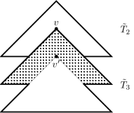
Figure 6: Construction of $\tilde{T}_{1},\tilde{T}_{2},\tilde{T}_{3}$ from $D_{s+1}$, in the proof of Proposition 20. The dotted part (to be pumped as $\tilde{T}_{1}$ between $\tilde{T}_{2}$ and $\tilde{T}_{3}$) is replaced with the tree-decomposition $\tau^{\prime}_{i}$ of $\sigma^{\prime}_{i}$ corresponding to representative $\sigma_{i}$ equivalent to $\mathcal{N}(v)$, with $i\in[s^{\prime}]$.

See Figure 6. With appropriate ports taken as the bags of $v$ and $v^{\prime}$, we have $\tilde{T}_{2}\oplus\tilde{T}_{3}=D_{s+1}$. By [10, Lemma 14] we deduce that $\Lambda^{\mathcal{T}}(2\cdot 1^{\ell}\cdot 3)$ is positive for $\psi$ for all $\ell\in\mathbb{N}$, and by Remark 2 there exist $\tilde{\Gamma}=\{\tilde{G}_{1},\tilde{G}_{2},\tilde{G}_{3}\}$ associated respectively to $\tilde{T}_{1},\tilde{T}_{2},\tilde{T}_{3}$ such that $\Delta^{\tilde{\Gamma}}(2\cdot 1^{\ell}\cdot 3)$ is a model of $\psi$ for all $\ell\in\mathbb{N}$. By construction we still have $P_{1}(\tilde{G}_{1})\cap P_{2}(\tilde{G}_{1})\neq V(\tilde{G}_{1})$, and furthermore $\tilde{G}_{2}\oplus\tilde{G}_{3}=M_{s+1}$ hence it is a $q$-uniform model of size greater than $q^{x}$, and finaly $\tilde{G}_{1}=\sigma^{\prime}_{i}$ (in the construction on tree-decompositions, the pumped part is replaced by $\tau^{\prime}_{i}$ corresponding to the graph $\sigma^{\prime}_{i}$). ∎

6.3 Assembling $q$-uniform networks

We prove Theorem 1.b, 1.d for any $q\geq 2$, based on arithmetical considerations generalizing the case $q=2$ presented in Subsection 5.2. The proof structure consists in applying Proposition 20 to obtain three $(k+1)$-graphs, then incorporte the saturating graph $\Omega_{m}$, and finaly reduce from SAT or UNSAT by constructing automata networks whose sizes are powers of $q$, thanks to the arithmetics from Theorem 10.

One may remark from the condition of Proposition 20 on the size of $\tilde{G}_{2}\oplus\tilde{G}_{3}$ that the case $\ell=0$ will be important, and justifies its consideration in Section 5. It is required by our reasoning, in order to control the size of the initial solution to ${\mathcal{P}_{q}(a,b)}$.

The other key ingredient consists in replacing the pumped part by its representative among $\{\sigma^{\prime}_{i}\}_{i\in[s^{\prime}]}$, which allows to bound the value of $a$ and apply Proposition 20 with a value of $x$ suitable for the subsequent use of the equivalent condition given by Theorem 19 for the application of Theorem 10.

Proof of Theorem 1.b, 1.d.

The proof structure is analogous to Theorem 1 for $q=2$, with additionnal considerations to apply the arithmetics from Section 5. The deterministic case is handled with the addition of $\chi$ as in Section 4, in order to have graphs of out-degree $1$ all the way.

Let $q\geq 2$, and $\psi$ be a $q$-arborescent (or $q$-non-trivial) MSO formula of rank $m$. Without loss of generality, assume that the saturating graph $\Omega_{m}$ from Proposition 2 (or Corollary 3) is a counter-model of $\psi$, and let us build a reduction from UNSAT (otherwise consider $\neg\psi$ instead of $\psi$, and a reduction from SAT instead of UNSAT).

Before calling Proposition 20, we setup an apropriate value of $x$ to ensure that the condition of Theorem 19 will be verified. It is related to the value of $a$ which is the size of the glued part, i.e. $\sigma^{\prime}_{i}$ from the Proposition. Recall that $\oplus$ merges the ports, of size $k$ in our context. Let $\eta$ be a value greater or equal to the maximum coprime power of $q$ for $\{|\sigma^{\prime}_{i}|-k\mid i\in[s^{\prime}]\}$, and also greater or equal to $\max\{\log_{q}(|\sigma^{\prime}_{i}|-k)\mid i\in[s^{\prime}]\}$.

Applying Proposition 20 for $x=\eta$, we obtain three $k$-graphs $\tilde{\Gamma}=\{\tilde{G}_{1},\tilde{G_{2}},\tilde{G}_{3}\}$, with $\tilde{G}_{1}=\sigma^{\prime}_{i}$ for some $i\in[s^{\prime}]$, such that $\Delta^{\tilde{\Gamma}}(2\cdot 1^{\ell}\cdot 3)\models\psi$ for all $\ell\in\mathbb{N}$. From $P_{1}(\tilde{G}_{1})\cap P_{2}(\tilde{G}_{1})\neq V(\tilde{G}_{1})$ we deduce the existence of $(a,b)\in\mathbb{N}_{+}\times\mathbb{N}$ with:

• $b=|\tilde{G}_{2}\oplus\tilde{G}_{3}|=q^{N}$ for some $N\geq\eta$,

• $a=|\tilde{G}_{1}|-k=|\sigma^{\prime}_{i}|-k$.

We have $|\Delta^{\tilde{\Gamma}}(2\cdot 1^{\ell}\cdot 3)|=a\ell+b$, which is a power of $q$ for $\ell=0$, i.e. we have the initial solution $(0,N)$ to ${\mathcal{P}_{q}(a,b)}$. Since this solution verifies that the coprime power of $q$ for $a$ is smaller than $N$, by Theorem 19 there exists a couple $(\mu,\kappa)\in\mathbb{N}_{+}\times\mathbb{N}_{+}$ such that we can apply Theorem 10, and deduce that ${\mathcal{P}_{q}(a,b)}$ contains a geometric sequence of integers. More precisely, from the proof of Lemma 15, in $\Delta^{\tilde{\Gamma}}(2\cdot 1^{\ell}\cdot 3)$ we have graphs of size $q^{N+\ell^{\prime}\mu}=bq^{\ell^{\prime}\mu}$ for all $\ell^{\prime}\in\mathbb{N}$, which correspond to $\ell=\frac{bq^{\ell^{\prime}\mu}-b}{a}$ being an integer (the number of copies of $\tilde{G}_{1}$).

Before continuing, let us consider the fourth graph. Let $\tilde{G_{0}}=\Omega_{m}\sqcup\tilde{G_{1}}$. Let $\alpha$ be the least power of $q$ such that $G_{1}=\bigoplus_{i=1}^{\alpha}\tilde{G}_{1}$ verifies $|G_{1}|\geq|\tilde{G}_{0}|$, and let $G_{0}$ be the disjoint union of $\tilde{G}_{0}$ and $|G_{1}|-|\tilde{G}_{0}|$ fixed points, so that $|G_{0}|=|G_{1}|$. Finaly, let $G_{2}=\tilde{G}_{2}$ and $G_{3}=\tilde{G}_{3}$. The $k$-graphs $\Gamma=\{G_{0},G_{1},G_{2},G_{3}\}$ verify Conditions 1–3 of Proposition 4, as usual. Furthermore, $G_{1}$ is made of $\alpha$ copies of $\tilde{G}_{1}$.

Given a propositional formula $S$ on $s$ variables, we need at least $2^{s}$ copies of $G_{0}$ or $G_{1}$ in order to implement the reduction from UNSAT, where for each valuation the circuit of the AN (resp. NAN) builds a copy of $G_{0}$ if $S$ is satisfied, and a copy of $G_{1}$ otherwise. Recall that $G_{1}$ is made of $\alpha$ copies of $\tilde{G}_{1}$ and $|G_{0}|=|G_{1}|$, that is, for $|w|=2^{s}$ we have $|\Delta^{\Gamma}(2\cdot w\cdot 3)|=a\alpha 2^{s}+b$. The goal is now to find a suitable padding by $L(s)$ copies of $\tilde{G}_{1}$, i.e. such that:

$$|\Delta^{\Gamma^{\prime}}(2\cdot w\cdot 4^{L(s)}\cdot 3)|=a(\alpha 2^{s}+L(s))+b$$

is a power of $q$, with $|w|=2^{s}$, $G_{4}=\tilde{G}_{1}$ and $\Gamma^{\prime}=\{G_{0},G_{1},G_{2},G_{3},G_{4}\}$. Then the reduction is as usual: the graph $\Delta^{\Gamma^{\prime}}(2\cdot w\cdot 4^{L(s)}\cdot 3)$ is a model of $\psi$ if and only if $w$ does not contain letter $0$ (in this case it has only copies of $\tilde{G}_{1}$). Remember that the only non-constant part is $S$ (and $s$).

We want to find $\ell^{\prime}\in\mathbb{N}$ such that:

$$\alpha 2^{s}+L(s)=\frac{bq^{\ell^{\prime}\mu}-b}{a}\iff L(s)=\frac{b}{a}(q^{\ell^{\prime}\mu}-1)-\alpha 2^{s}.$$

A solution with $L(s)\geq 0$ is $\ell^{\prime}=s+\log_{q}(\alpha)+1$. Indeed, we have $\frac{b}{a}\geq 1$ by the hypothesis on $\eta$ (upper bounding $a$) and $b=q^{\eta}$. Then $q^{\ell^{\prime}\mu}\geq\alpha 2^{s}+1$ is verified by $\ell^{\prime}$ because $\mu\geq 1$ and $q\geq 2$.

Therefore, we can build a Boolean NAN (or AN) with

$$n=\log_{q}(b)+\mu(s+1)+\mu\log_{q}(\alpha)$$ automata, and

$$\alpha 2^{s}+L(s)=\frac{bq^{\mu(s+1)}\alpha^{\mu}-b}{a} \tilde{G}_{1}$$ copies of

(some copies of $\tilde{G}_{1}$ form copies of $G_{1}$, or are replaced by a copy of $G_{0}$ when $S$ is satisfied). Recall that $a$, $b$, $\mu$ and $\alpha$ are constants depending only on $\psi$. ∎

7 Conclusion and perspectives

We have proven Theorem 1, that any non-trivial (in the deterministic setting) or arborescent (in the non-deterministic setting) MSO question on the dynamics of a given automata network (AN) or non-deterministic automata network (NAN) is ${\mathsf{NP}}$-hard or ${\mathsf{coNP}}$-hard to answer, when given the network’s description in the form of a circuit, even in the case of bounded alphabets. Part c of Theorem 1 was proven in [10], on which our developments are grounded. In Section 4 we have included the deterministic constaint to the abstract pumping technique in order to obtain Theorem 1.a. In Section 5 we have treated the arithmetics of the intersection between the sizes of $q$-uniform automata networks, and the sizes of models obtained by pumping. This led to the proof of Theorem 1.b, 1.d in Section 6. In particular, the Rice-like complexity lower bounds also hold for Boolean (deterministic and non-deterministic) automata networks, a model widely used in applications to system biology, for example in the study of gene regulatory networks. Our results intuitively state that any “interesting” computational investigation of the dynamics in a model of interacting entities, is limited to a “high” time-complexity cost in the worst case. Hence there cannot exist any general efficient algorithm, unless some unsuspected complexity collapse occurs (such as ${\mathsf{P}}={\mathsf{NP}}$).

The deterministic case is now closed for MSO (remark that deterministic implies treewidth at most $2$), because the trivial versus non-trivial dichotomy is sharp and deep: all trivial formulas are answers with $\mathcal{O}(1)$ algorithms, whereas all non-trivial formulas are hard for the first level of the polynomial hierarchy (either ${\mathsf{NP}}$ or ${\mathsf{coNP}}$). However, in the non-deterministic case there are computationaly hard non-arborescent formulas (e.g. being a clique), hence the dichotomy does not reaches the sharpness of an “a la Rice” statement. To go further, it would be meaningful to extend the proof technique to other structural graph parameters, such as cliquewidth, rankwidth and twinwidth. In [10], it is formally argued that graph parameterization is necessary to derive general complexity lower bounds for non-deterministic automata networks, because a proof of the basic trivial versus non-trivial dichotomy in this setting implies unexpected complexity collapses (regardless of our considerations on alphabet sizes, and even at first-order).

The definition of non-determinism we have employed is global, and in the uniform case it does not accommodate the Cartesian product of local possibilities (in the case of unrestricted alphabets it does, simply by considering automata networks of size $n=1$, with potentially huge alphabets). Could the abstract pumping technique be applied to such a notion of local non-determinism ?

A result of [9] is that there are first order questions complete at all levels of the polynomial hierarchy (even in the deterministic case), therefore obtaining general lower bounds at higher levels seems another pertinent track to follow, where a good notion of “highly non-trivial” formula needs to be established.

Finally, the signature of our logics contain (appart from the $\in$ of MSO) only the two binary relations $\{=,\to\}$ on pairs of configurations (vertices), consequently all expressible questions are valid up to graph isomorphism. Distinguishing configurations may be meaningful for applications, therefore the addition of finer relations is another interesting research track to expand the results.

References

- [1] N. Alon. Asynchronous threshold networks. Graphs and Combinatorics, 1:305––310, 1985.
- [2] J. Aracena, F. Bridoux, L. Gómez, and L. Salinas. Complexity of limit cycles with block-sequential update schedules in conjunctive networks. Natural Computing, 22(3):411–429, 2023.
- [3] F. Bridoux, C. Gaze-Maillot, K. Perrot, and S. Sené. Complexity of limit-cycle problems in boolean networks. In Proceedings of SOFSEM’2021, volume 12607 of LNCS, pages 135–146. Springer, 2021.
- [4] A. Dennunzio, E. Formenti, E. Manzoni, G. Mauri, and A. E. Porreca. Computational complexity of finite asynchronous cellular automata. Theoretical Computer Science, 664:131–143, 2017.
- [5] R. G. Downey, M. R. Fellows, et al. Fundamentals of parameterized complexity, volume 4. Springer, 2013.
- [6] C. Espinosa-Soto, P. Padilla-Longoria, and E. R. Alvarez-Buylla. A gene regulatory network model for cell-fate determination during Arabidopsis thaliana flower development that is robust and recovers experimental gene expression profiles. The Plant Cell, 16:2923–2939, 2004.
- [7] P. Floreen and P. Orponen. On the computational complexity of analyzing Hopfield nets. Complex Systems, 3:577–587, 1989.
- [8] E. Formenti and K. Perrot. How Hard is it to Predict Sandpiles on Lattices? A Survey. Fundamenta Informaticae, 171:189–219, 2019.
- [9] G. Gamard, P. Guillon, K. Perrot, and G. Theyssier. Rice-Like Theorems for Automata Networks. In Proceedings of STACS’2021, volume 187 of LIPIcs, pages 32:1–32:17. Schloss Dagstuhl, 2021.
- [10] G. Gamard, P. Guillon, K. Perrot, and G. Theyssier. Hardness of monadic second-order formulae over succinct graphs. Preprint arXiv:2302.04522v2, 2024.
- [11] E. Goles and P. Montealegre. The complexity of the asynchronous prediction of the majority automata. Information and Computation, 274:104537, 2020.
- [12] E. Goles, P. Montealegre, K. Perrot, and G. Theyssier. On the complexity of two-dimensional signed majority cellular automata. Journal of Computer and System Sciences, 91:1–32, 2018.
- [13] E. Goles, P. Montealegre, M. Ríos Wilson, and G. Theyssier. On the impact of treewidth in the computational complexity of freezing dynamics. In Proceedings of CiE’2021, pages 260–272. Springer, 2021.
- [14] D. Griffeath and C. Moore. Life Without Death is P-complete. Complex Systems, 10, 1996.
- [15] G. Karlebach and R. Shamir. Modelling and analysis of gene regulatory networks. Nature Reviews Molecular Cell Biology, 9:770–780, 2008.
- [16] S. A. Kauffman. Metabolic stability and epigenesis in randomly constructed genetic nets. Journal of Theoretical Biology, 22:437–467, 1969.
- [17] S. Kosub. Dichotomy results for fixed-point existence problems for Boolean dynamical systems. Mathematics in Computer Science, 1:487––505, 2008.
- [18] C. Lhoussaine and E. Remy. Symbolic Approaches to Modeling and Analysis of Biological Systems. ISTE Consignment. Wiley, 2023.
- [19] L. Libkin. Elements of Finite Model Theory. Springer, 2004.
- [20] J. Machta and K. Moriarty. The computational complexity of the Lorentz lattice gas. Journal of Statistical Physics, 87(5):1245–1252, 1997.
- [21] L. Mendoza and E. R. Alvarez-Buylla. Dynamics of the genetic regulatory network for Arabidopsis thaliana flower morphogenesis. Journal of Theoretical Biology, 193:307–319, 1998.
- [22] C. Moore. Majority-Vote Cellular Automata, Ising Dynamics, and P-Completeness. Journal of Statistical Physics, 88(3):795–805, 1997.
- [23] C. Moore and M. Nilsson. The Computational Complexity of Sandpiles. Journal of Statistical Physics, 96:205–224, 1999.
- [24] C. Moore and M. G. Nordahl. Predicting lattice gases is P-complete. Technical report, Santa Fe Institute Working Paper 97-04-034, 1997.
- [25] T. Neary and D. Woods. P-completeness of Cellular Automaton Rule 110. In Proceedings of ICALP’2016, volume 4051 of LNCS, pages 132–143, 2006.
- [26] C. Noûs, K. Perrot, S. Sené, and L. Venturini. #P-completeness of counting update digraphs, cacti, and series-parallel decomposition method. In Proceedings of CiE’2020, volume 12098 of LNCS, pages 326–338. Springer, 2020.
- [27] P. Orponen. Neural networks and complexity theory. In Proceedings of MFCS’1992, volume 629 of LNCS, pages 50–61, 1992.
- [28] E. Palma, L. Salinas, and J. Aracena. Enumeration and extension of non-equivalent deterministic update schedules in boolean networks. Bioinformics, 32(5):722–729, 2016.
- [29] L. Paulevé and S. Sené. Systems biology modelling and analysis: formal bioinformatics methods and tools, chapter Boolean networks and their dynamics: the impact of updates, pages 173–250. Wiley, 2022.
- [30] H. G. Rice. Classes of recursively enumerable sets and their decision problems. Transactions of the American Mathematical Society, 74:358–366, 1953.
- [31] L. Salinas, L. Gómez, and J. Aracena. Existence and non existence of limit cycles in boolean networks. In Automata and Complexity, volume 42, pages 233–252. Springer, 2022.
- [32] K. Sutner. The computational complexity of cellular automata. In Proceedings of FCT’1989, page 451–459. Springer-Verlag, 1989.
- [33] D. Thieffry and R. Thomas. Dynamical behaviour of biological regulatory networks – II. Immunity control in bacteriophage lambda. Bulletin of Mathematical Biology, 57:277–297, 1995.
- [34] R. Thomas. Boolean formalization of genetic control circuits. Journal of Theoretical Biology, 42:563–585, 1973.