Tilted Solid-On-Solid is liquid:
scaling limit of SOS with a potential on a slope

Abstract.

The $(2+1)$d Solid-On-Solid (SOS) model famously exhibits a roughening transition: on an $N\times N$ torus with the height at the origin rooted at $0$, the variance of $h(x)$, the height at $x$, is $O(1)$ at large inverse-temperature $\beta$, vs.  $\asymp\log|x|$ at small $\beta$ (as in the Gaussian free field (GFF)). The former—rigidity at large $\beta$—is known for a wide class of $|\nabla\phi|^{p}$ models ($p=1$ being SOS) yet is believed to fail once the surface is on a slope (tilted boundary conditions). It is conjectured that the slope would destabilize the rigidity and induce the GFF-type behavior of the surface at small $\beta$. The only rigorous result on this is by Sheffield (2005): for these models of integer height functions, if the slope $\theta$ is irrational, then $\operatorname{Var}(h(x))\to\infty$ with $|x|$ (with no known quantitative bound).

We study a family of SOS surfaces at a large enough fixed $\beta$, on an $N\times N$ torus with a nonzero boundary condition slope $\theta$, perturbed by a potential $\mathsf{V}$ of strength $\varepsilon_{\beta}$ per site (arbitrarily small). Our main result is (a) the measure on the height gradients $\nabla h$ has a weak limit $\mu_{\infty}$ as $N\to\infty$; and (b) the scaling limit of a sample from $\mu_{\infty}$ converges to a full plane GFF. In particular, we recover the asymptotics $\operatorname{Var}(h(x))\sim c\log|x|$. To our knowledge, this is the first example of a tilted $|\nabla\phi|^{p}$ model, or a perturbation thereof, where the limit is recovered at large $\beta$. The proof looks at random monotone surfaces that approximate the SOS surface, and shows that (i) these form a weakly interacting dimer model, and (ii) the renormalization framework of Giuliani, Mastropietro and Toninelli (2017) leads to the GFF limit. New ingredients are needed in both parts, including a nontrivial extension of [GMT17] from finite interactions to any long range summable interactions.

1. Introduction

The Solid-On-Solid (SOS) model on a finite graph with vertices ${\mathcal{V}}$ and edges ${\mathcal{E}}$ is a distribution on height functions $h:{\mathcal{V}}\to\mathbb{Z}$ rooted at a marked vertex $o$ (the origin) to $h(o)=0$. The probability assigned to each $h$ penalize it for having large (in absolute value) gradients along the edges $e\in{\mathcal{E}}$:

$$\mathbb{P}_{\beta}(h)\propto\exp\Big{[}-\beta\sum_{e\in{\mathcal{E}}}\left|\nabla h(e)\right|\Big{]}\,,$$

where $\nabla h(e):=h(y)-h(x)$ for $e=(x,y)\in{\mathcal{E}}$ and the parameter $\beta>0$ is the inverse-temperature.

The $(2+1)$d SOS model takes the graph to be the $N\times N$ torus in $\mathbb{Z}^{2}$, denoted here $\Lambda_{N}$, where the heights are assigned to the $N^{2}$ unit-squares. Note that $\mathbb{P}_{\beta}$ is then translation-invariant (as the torus is vertex transitive, and rooting $h(o)=0$ has no effect when we only look at the gradients $\nabla h$). One associates to $h$ the surface in $\mathbb{R}^{3}$ consisting of a horizontal face of $\mathbb{Z}^{3}$ at height $h(x)$ for each $x\in{\mathcal{V}}(\Lambda_{N})$ and a minimum completion of vertical faces to make them simply connected (i.e., $|\nabla h(e)|$ faces for each $e\in{\mathcal{E}}(\Lambda_{N})$). Viewing $h$ as this set of faces, $|h|=N^{2}+\sum_{e\in{\mathcal{E}}}|\nabla h(e)|$, thus

$$\mathbb{P}_{\beta}(h)\propto\exp\big{(}-\beta|h|\big{)}\,.$$ (1.1)

The study of this model in statistical physics goes back to the early 1950’s ([12, 55]), pertaining crystal formation at low temperature (large $\beta$). It further serves as an approximation of plus/minus interfaces in the 3d Ising model, which resemble a height functions as overhangs are microscopic in that regime. In line with predictions for 3d Ising (given in the 1970’s, remain unproved: cf. [1, 24]), the $(2+1)$d SOS model undergoes a roughening transition from being delocalized, or rough (formally defined below) at small $\beta$ to localized, or rigid at large $\beta$. It is widely believed that for 3d Ising and its approximations, e.g., $(2+1)$d SOS and more general $|\nabla\phi|^{p}$ models, when the interface is on a slope, the rigidity at large $\beta$ is destabilized, mirroring the small $\beta$ behavior (see Figs. 1 and 2).

In this work we give a first rigorous proof of the scaling limit of such a model at large $\beta$ on a slope: we show that the $(2+1)$d SOS model perturbed by a potential of $\varepsilon_{\beta}$ per site converges to a GFF. As we further explain below, it was unclear whether the scaling limit of tilted Ising-type interfaces would in fact match the zero temperature GFF picture, especially if the nonzero slope is rational.

There is a vast body of works on low temperature 3d Ising interfaces and $(2+1)$d SOS surfaces, intrinsic to the study of crystals. In the physics literature there are numerous studies, experimental (e.g., [4] comparing roughening in ${}^{4}\mathrm{He}$ crystals to 3d Ising) and theoretical (e.g., [58] drawing evidence for the existence of a roughening transition in 3d Ising); see [39, 33, 54, 19, 23, 41, 52, 51, 50] as well as [57] and the references therein, for a sample of such studies going back to the early 1950’s. The mathematical physics literature, aside from the celebrated work of Fröhlich and Spencer [25] that we expand on below, has been mostly confined to the rigid regime of these models—starting from the pioneering work of Dobrushin [22] in the early 1970’s and proceeding to delicate aspects such as entropic repulsion, layering and wetting; see, e.g., [11, 2, 46, 47, 14, 15, 21, 17, 18] for but a small sample, as well as some recent works [13, 29, 30, 32, 31, 28] and the survey [40] and references therein.

Figure 1. Simulation of a $(2+1)$d SOS model on a $500\times 500$ box with slope $\theta=(1,1)$ at inverse-temperature $\beta=3$, with a marked $100\times 100$ region zoomed in on the left.

Figure 2. The $(2+1)$d SOS surface from Fig. 1 after centering it about the mean heights.

That the surface in the rough phase should have logarithmic fluctuations/correlations appears in many of these works; as for its continuum scaling limit, Fröhlich, Pfister and Spencer [24] wrote in 1981 (see p. 186 there) that it should be “given by massless Gaussian measures.”

Following the landmark result of Kenyon [43] that for 3d Ising at zero temperature ($\beta=\infty$) under tilted boundary conditions, the scaling limit of the interface is the Gaussian free field (GFF) (see also [42, Theorem 15], [44, Sec. 3] and [45] which covers any planar graph), various works asked if this should be the scaling limit also at finite $\beta$; see, e.g., the discussions in [9, 37] and the following excerpt, pertaining to a slope $\theta=(1,1)$, in the recent work of Giuliani, Renzi and Toninelli [36]: “It is very likely that the GFF behavior survives the presence of a small but positive temperature; however, the techniques underlying the proof at zero temperature, based on the exact solvability of the planar dimer problem, break down.”

The roughness of the interface in the tilted $(2+1)$d SOS model, at least for an irrational slope $\theta$, is rigorously known (unlike 3d Ising at low temperature), yet this model remains highly nontrivial; e.g., in 2001, Bodineau, Giacomin and Velenik [9] considered interfaces that have a slope $\theta=(\theta_{1},0)$, stating “…the most natural effective model should have been the SOS model. However, only few results have been obtained about the fluctuations of this model, because the singularity of the interaction does not allow to use the techniques based on strict convexity of the potential.” Velenik [56], in his comprehensive survey from 2006 (that also covers $\mathbb{R}$-valued (continuous) models, where there is no parameter $\beta$; see, e.g., the recent work [3]) wrote that, for the SOS model with any nonzero slope, it is expected that “the large-scale behavior of these random interfaces is identical to that of their continuous counterpart. In particular they should have Gaussian asymptotics. This turns out to be quite delicate… I am not aware of a single rigorous proof for finite $\beta$.”

Figure 3. Roughening transition: $(2+1)$d Solid-On-Solid on a $64\times 64$ box at different $\beta$ with flat boundary conditions; sampled via $10^{4}$ steps of Glauber dynamics started at all-$0$.

Let us now formally describe what is known on roughening in the SOS model (depicted in Fig. 3). The roughening transition can be observed in the behavior of $\operatorname{Var}(h(x))$ as $|x|\to\infty$, where $|x|$ is the Euclidean distance of the site $x$ from the origin $o$ (at which the surface is rooted at $0$). In 1981, Fröhlich and Spencer [25] famously proved that $\operatorname{Var}(h(x))\asymp\log|x|$ at small $\beta$, as in the GFF, the conjectured scaling limit in this regime. Conversely, a Peierls-type argument (see Branderberger and Wayne [10]) shows $\operatorname{Var}(h(x))=O(1)$ at large $\beta$. (A recent breakthrough result by Lammers [48] proved sharpness of this transition: for some $\beta_{\textsc{r}}$, the former holds for $\beta\leq\beta_{\textsc{r}}$, the latter for $\beta>\beta_{\textsc{r}}$.)

The $|\nabla\phi|^{p}$-models ($p\geq 1$) generalize SOS (the case $p=1$) into $\mathbb{P}_{\beta}(h)\propto\exp[-\beta\sum_{e\in{\mathcal{E}}}|\nabla h(e)|^{p}]$. All these models are expected to demonstrate similar behavior, including the roughening transition; and while the Fröhlich–Spencer argument only applies to $p=1,2$, the Peierls argument of [10] (cf. [26]) applies to all $p\geq 1$. (See [49] for more on similarities between these models at large $\beta$.) However, this Peierls argument, albeit quite robust, only addresses contractible level line loops, and thus ceases to imply rigidity at large $\beta$ when the surface is positioned on a slope.

Figure 4. SOS configuration on a $10\times 10$ torus, extended periodically with slope $\theta=(1,1)$.

We now define the precise setup of periodic boundary conditions for $(2+1)$d SOS with slope $\theta$. The $(2+1)$d SOS model on the $N\times N$ torus $\Lambda_{N}$ with slope $\theta=(\theta_{1},\theta_{2})$, which without loss of generality has $\theta_{1},\theta_{2}\geq 0$, is formally obtained by extending the function $h$ to $\mathbb{Z}^{2}$ periodically, decreasing it by $\lfloor\theta_{1}N\rfloor$ along the $(1,0)$-direction and by $\lfloor\theta_{2}N\rfloor$ in the $(0,1)$-direction (see Fig. 4). That is, one views $h$ as a full plane height function, where for every face $x=(x_{1},x_{2})$ of $\mathbb{Z}^{2}$,

$$h(x_{1}+N,x_{2})=h(x_{1},x_{2})-\lfloor\theta_{1}N\rfloor\quad\mbox{and}\quad h(x_{1},x_{2}+N)=h(x_{1},x_{2})-\lfloor\theta_{2}N\rfloor\,.$$ (1.2)

Equivalently, one restricts the height functions $h$ on the torus to those where $\sum\nabla h(\vec{e}_{i})=-\lfloor\theta_{1}N\rfloor$ for every non-contractible loop of directed edges $(\vec{e}_{i})$ in the $(1,0)$-direction, and $\sum\nabla h(\vec{e}_{i})=-\lfloor\theta_{2}N\rfloor$ for non-contractible loops in the $(0,1)$-direction (and $\sum\nabla h(\vec{e}_{i})=0$ for every contractible loop). (Formally, in this formulation one only considers the $1$-form/vector-field $\nabla h$ as opposed to $h$.) From this definition, we see that the SOS measure on the torus with slope $\theta$ is translation-invariant.

The slope $\theta=(\theta_{1},\theta_{2})$ deterministically induces $(\theta_{1}+\theta_{2})N$ macroscopic level line loops in the SOS surface (see Section 2.1 for a formal definition), each one a non-contractible loop, thus unaddressed by the rigidity Peierls argument (which is only applicable to contractible level line loops). Indeed, these interacting macroscopic level lines (which cannot cross one another) break the surface rigidity and are conjectured to yield a GFF scaling limit (as also conjectured for the flat setup at small $\beta$).

A beautiful result of Sheffield [53] from 2005 shows that the SOS surface with slope $\theta$ on a torus is rough when $\theta=(\theta_{1},\theta_{2})$ is irrational in one of its coordinates. Precisely, via a highly nontrivial application of the Ergodic Theorem, Sheffield proved that there does not exist an ergodic and translation-invariant Gibbs measure $\mu_{\theta}$ for the height function $h$ with an irrational slope $\theta$ (where $\theta_{i}(\mu):=\mathbb{E}_{\mu}\nabla h(\vec{e}_{i})$ for $\vec{e}_{1}=(o,o+(1,0))$, $\vec{e}_{2}=(o,o+(0,1))$; both are integrable by assumption). It thus follows that $\operatorname{Var}(h(x))\to\infty$, since otherwise having $\operatorname{Var}(h(x))=O(1)$ would have implied (through tightness and routine reasoning) the existence of an ergodic and translation-invariant subsequential local limit. Sheffield’s argument is remarkably general: it is applicable to a wide family of nearest-neighbor translation-invariant models of integer height functions on $\mathbb{Z}^{2}$, including, e.g., all $|\nabla\phi|^{p}$ ($p\geq 1$) models; thus, the random surfaces in all these models are rough when the slope $\theta$ is irrational. However, this argument gives no bound on the rate of $\operatorname{Var}(h(x))$ as $|x|\to\infty$.

In recent years, significant progress was made in the study of $(2+1)$d $|\nabla\phi|^{p}$ models in the flat setup $(\theta=0)$ (cf., the aforementioned work of Lammers [48] on the phase transition in SOS; and the recent breakthrough of Bauerschmidt et al. [5, 6] on the convergence of the Discrete Gaussian model (the case $p=2$) to a GFF at high enough temperatures). However, at low temperature and with a nonzero slope $\theta$, the only known result remains the work of Sheffield [53] described above.

In this work we study the $(2+1)$d SOS model of Eq. 1.1 on a torus with slope $\theta=(\theta_{1},\theta_{2})$, for any $\theta_{1},\theta_{2}>0$, with a pinning-type potential $\mathsf{V}$ (out of a given family of potentials defined below):

$$\mathbb{P}_{\beta,\lambda}(h)=\frac{1}{{\mathcal{Z}}^{\textsc{sos}}_{N,\beta,\lambda}}\exp\left[-\beta|h|-\lambda\mathsf{V}(h)\right]\,.$$ (1.3)

We stress that the potential strength $\lambda>0$ can be taken as $\varepsilon_{\beta}$, arbitrarily small for large enough $\beta$ (whereas the potential $\mathsf{V}$ will be assigning a cost of either $0$ or $1$ per face of the SOS surface $h$); thus, one expects the surface behavior to be governed by its energy $\beta|h|$ and entropy, as in $\lambda=0$.

The $(2+1)$d SOS model with flat boundary conditions ($\theta=0$) was studied in detail under a pinning potential (see the survey [40] and the recent works by Lacoin [46, 47]) that rewards every face of $h$ intersecting a preset plane, typically the slab at height $0$—the ground state of the model. The SOS model with a nonzero slope $\theta$, on the other hand, has exponentially many ground states (monotone surfaces, as we explain next); accordingly, our family of pinning potentials will reward the overlap of $h$ not with a predetermined ground state, but rather with its “closest” ground state.

We say that an SOS height function $h$ is a monotone surface if $h(x_{1},x_{2})\geq h(y_{1},y_{2})$ whenever $y_{1}\geq x_{1}$ and $y_{2}\geq x_{2}$. We will often denote a monotone surface by $\varphi$ or $\psi$, and refer to it as a tiling, owing to the well-known bijection between monotone surfaces in $\mathbb{Z}^{2}$ and lozenge tilings of the triangular lattice $\mathbb{T}$ (as well as with dimers in the hexagonal lattice; see below for more details). We impose on the tiling the same periodic conditions with slope $\theta$ as in Eq. 1.2. It is easy to see that, out of all periodic SOS surfaces $h$ with slope $\theta$, tilings minimize $|h|$, the number of faces (recalling $|h|=N^{2}+\sum|\nabla h(e)|$); that is, tilings are the ground states for the model at $\lambda=0$.

The potentials $\mathsf{V}$ studied here will pin $h$ to $\psi_{0}$, the closest tiling to it in terms of common faces. (We do not root $\psi_{0}$ to be $0$ at the origin, as it will intersect $h$ which is already rooted.) We give two concrete examples of such a $\mathsf{V}$ before describing the general family of potentials considered.

Example 1.1 (pinning to a closest tiling).

Consider all tilings $\psi_{0}$ satisfying Eq. 1.2, and set

$$\mathsf{V}_{1}(h)=\min_{\psi_{0}}|\psi_{0}\setminus h|\,.$$ (1.4)

(This is equivalent to taking $\mathsf{V}_{1}(h)=-\max_{\psi_{0}}|h\cap\psi_{0}|$; every face in $h\cap\psi_{0}$ collects a reward of $\lambda$.)

Note that when $\theta=0$ (no slope), the only tiling $\psi_{0}$ compatible with the boundary conditions is the flat one, whence $\mathsf{V}_{1}$ coincides with the classical pinning potential (rewarding faces at height $0$).

Example 1.2 (truncated pinning to a tiling).

Let $\psi_{0}$ be a minimizer of $|\psi_{0}\setminus h|$ (attaining Eq. 1.4, arbitrarily chosen if multiple exist), and $\{S_{i}\}$ be the connected components of faces of $\psi_{0}\setminus h$. Set

$$\mathsf{V}_{2}(h)=\sum|S_{i}|\mathbbm{1}_{\{|S_{i}|\geq 1000\}}\,.$$ (1.5)

Definition 1.3 (family of pinning potentials).

Consider a tiling $\psi_{0}$ minimizing $|\psi_{0}\setminus h|$ (a canonical way to break ties will be given in Proposition 4.1) and fix an arbitrarily large $\mathsf{M}_{0}$ (e.g., $\mathsf{M}_{0}=1000$). The potential $\mathsf{V}$ can be any function of a (maximal) connected component $S$ of $\psi_{0}\setminus h$, which counts $0$ or $1$ for each face of $S$, such that it collects at least $\lfloor|S|/\mathsf{M}_{0}\rfloor$ faces of the component. Precisely,

$$\mathsf{V}(h)=\sum f(S_{i})\quad\mbox{for some function $f$ satisfying }\quad\lfloor|S|/\mathsf{M}_{0}\rfloor\leq f(S)\leq|S|\mbox{ for all $S$}\,,$$ (1.6)

where the sum goes over all the connected components $S_{i}$ of $\psi_{0}\setminus h$.

We stress that the potential $\mathsf{V}$ may ignore any component $S_{i}$ of $\psi_{0}\setminus h$ with less than $\mathsf{M}_{0}$ faces; i.e., it may penalize $h$ only for large regions missed by the best approximating ground state $\psi_{0}$. Such a potential $\mathsf{V}$ adds just enough noise to the model—even at $\lambda=\varepsilon_{\beta}$—to treat cases where close ground states have atypically large “frozen” regions, foiling the analysis of interacting tilings.

Figure 5. Level line comparison of the SOS surface vs. its centering from Figs. 1 and 2.

1.1. Main results

Our motivation was to recover the asymptotic rate of $\operatorname{Var}(h(o))$ in the SOS model of Eq. 1.3 at large $\beta$ and a nonzero slope $\theta$ (which, to our knowledge, is not known for any $|\nabla\phi|^{p}$ model with any added potential (of strength $\varepsilon_{\beta}$, so as not to compete with energy/entropy)). Our main result obtains this, and moreover establishes that (a) the law on $\nabla h$ around the origin $o$ converges to a full plane limit $\mu_{\infty}$; and (b) the scaling limit of $\mu_{\infty}$ converges to a full plane GFF. Recall that the full plane GFF is defined as a centered Gaussian stochastic process indexed by smooth compactly supported $\mathbb{C}\to\mathbb{R}$ functions with $0$ integral and covariance

$$\operatorname{Cov}\big{(}\textsc{GFF}(f_{1}),\textsc{GFF}(f_{2})\big{)}:=-\frac{1}{\pi^{2}}\int f_{1}(u)f_{2}(v)\log|u-v|\mathrm{d}u\mathrm{d}v\,,$$

where $\textsc{GFF}(f)$ is the value of the process at the function $f$, as in the expectation for a distribution.

Theorem 1.

For every $\lambda>0$ and $\theta_{1},\theta_{2}>0$ there exists $\beta_{0}$ so the following holds for every $\beta>\beta_{0}$. Consider the $(2+1)$d SOS model of Eq. 1.3, for any potential function $\mathsf{V}$ as per Definition 1.3, on $\Lambda_{N}$, an $N\times N$ torus with slope $\theta=(\theta_{1},\theta_{2})$ as defined in Eq. 1.2. Then

1. The law on the SOS gradients $\nabla h$ converges weakly, as $N\to\infty$, to a full plane limit $\mu_{\infty}^{\beta,\lambda}$.

2. Sample $h\sim\mu_{\infty}^{\beta,\lambda}$. There exist $\sigma>0$ and a linear map $\mathfrak{L}$ on $\mathbb{R}^{2}$ (nonrandom) such that

   $$h(n\,\cdot)-\mathbb{E}[h(n\,\cdot)]\xrightarrow[]{\;\mathrm{d}\;}\sigma\textsc{GFF}\circ\mathfrak{L}\quad\mbox{as $n\to\infty$}$$

   (viewing both sides as stochastic processes indexed by test functions with $0$ integral).

As the GFF is a distribution, Theorem 1 does not provide asymptotics of finite moments of the SOS height function $h$. However, building on its proof, one can derive those, as demonstrated next.

Corollary 2.

In the setting of Theorem 1, there exists $c>0$ such that

$$\operatorname{Var}(h(x))=(c+o(1))\log|x|\quad\mbox{as $|x|\to\infty$}\,.$$

The new results readily yield a law of large numbers (LLN) for $h(x)$, having $\sqrt{\log|x|}$ fluctuations about its mean $\theta\cdot x$ (see the level lines in Fig. 5 depicting the LLN). It is interesting to compare these results with the LLN for the shape of the Wulff crystal in 3d Ising near the corner of a box at zero temperature ($\beta=\infty$), due to Cerf and Kenyon [16], where lozenge tilings naturally appear.

The intuition behind the GFF scaling limit of the centered height function is that, at large $\beta$, the SOS surface $h$ should behave like a randomly perturbed “almost uniformly” chosen ground state (which, we recall, is a lozenge tiling of the triangular lattice $\mathbb{T}$). As mentioned above, a seminal result of Kenyon [43] established that the scaling limit of a uniform (domino) tiling is the GFF, whence one would expect that the SOS surface $h$ should inherit the same scaling limit.

Our proof strategy is to increase the probability space via a random tiling $\varphi$ conditional on $h$:

$$\mathbb{P}(\varphi\mid h)\propto\exp(+\alpha|h\cap\varphi|)$$

for some $\alpha>0$ (e.g., $\alpha=\beta$), rewarding $\varphi$ for faces in $h\cap\varphi$ (see Eq. 1.10), and establish that:

1. The marginal on $\varphi$ is a weakly interacting tiling, that is to say, it is a tilting of the uniform distribution of the following form: $\mathbb{P}(\varphi)\propto\exp\big{[}-\sum_{x}\sum_{r}\mathfrak{g}_{r}(\varphi\mathord{\upharpoonright}_{B(x,r)})\big{]}$, where $B(x,r)$ is the radius-$r$ ball around $x$ and $\mathfrak{g}_{r}$ are functions whose $L^{\infty}$-norm decays exponentially with $r$.

2. Consequently, via the powerful renormalization group machinery of Giuliani, Mastropietro and Toninelli [34, 35], the random tiling $\varphi$ has a scaling limit given by a GFF.

3. The SOS surface $h$ is a local perturbation of $\varphi$, thus has the same limit.

The aforementioned renormalization result of [34, 35] may be summarized as follows:

Theorem 1.4 ([34, 35]).

Fix $\mathfrak{a},\mathfrak{b},\mathfrak{c}>0$ to be three sides of a non-degenerate triangle and $R>0$. There exists $\delta>0$ (depending on $\mathfrak{a},\mathfrak{b},\mathfrak{c},R$) so that the following holds for every function $\mathfrak{g}$ on lozenge tilings of a ball of radius $R$ (with free boundary condition) in the triangular lattice $\mathbb{T}$ satisfying

$$\|\mathfrak{g}\|_{\infty}\leq\delta\,.$$ (1.7)

Let $\mu_{N}$ be distributions over tilings $\varphi$ of the torus $\mathbb{T}_{N}$ given by

$$\mu_{N}(\varphi)\propto\mathfrak{a}^{n_{\mathfrak{a}}(\varphi)}\mathfrak{b}^{n_{\mathfrak{b}}(\varphi)}\mathfrak{c}^{n_{\mathfrak{c}}(\varphi)}\exp\Big{[}\sum_{x}\mathfrak{g}(\varphi\mathord{\upharpoonright}_{B(x,R)})\Big{]}\quad\mbox{for all $N$}\,,\vspace{-3pt}$$

where $n_{\mathfrak{s}}(\varphi)$ counts the number of lozenges of type $\mathfrak{s}\in\{\mathfrak{a},\mathfrak{b},\mathfrak{c}\}$ in $\varphi$. Then:

1. $\mu_{N}\to\mu_{\infty}$ locally for the gradients $\nabla\varphi$ as $N\to\infty$; and

2. if $\varphi$ is sampled from $\mu_{\infty}$ and viewed as a height function projected on the plane ${\mathcal{P}}_{111}$, then

   $$\varphi(n\,\cdot)-\mathbb{E}[\varphi(n\,\cdot)]\xrightarrow[]{\;\mathrm{d}\;}\sigma\textsc{GFF}\circ\mathfrak{L}\,,$$

   where $\sigma>0$, $\mathfrak{L}$ is an invertible linear map and GFF is a full plane Gaussian free field.

The proof of Theorem 1.4 given in [34, 35] easily extends to the case where, instead of a single $\mathfrak{g}$ as per Eq. 1.7, there is a sequence of functions $(\mathfrak{g}_{r})$ on balls of growing radius $r\to\infty$, as long as

$$\|\mathfrak{g}_{r}\|_{\infty}\leq\delta\exp(-Cr^{2})\qquad\mbox{for a large enough constant }C>0\,.$$

Unfortunately, that assumption is much stronger than what our model affords: we can only hope for $\|\mathfrak{g}_{r}\|_{\infty}\leq O(e^{-cr})$, i.e., an exponential decay in the radius of the ball rather than in its volume. Several new ingredients were needed to boost Theorem 1.4 to the following, with a relaxed Eq. 1.8.

Theorem 3.

Fix $\mathfrak{a},\mathfrak{b},\mathfrak{c}>0$ to be three sides of a non-degenerate triangle, and let $\pi p_{\mathfrak{a}},\pi p_{\mathfrak{b}},\pi p_{\mathfrak{c}}$ denote its angles. For every $c>0$ there exists $\delta>0$ (depending on $\mathfrak{a},\mathfrak{b},\mathfrak{c},c$) such that the following holds for every sequence of functions $(\mathfrak{g}_{r})_{r=1}^{\infty}$ on lozenge tilings of balls of radius $r$ in $\mathbb{T}$ satisfying

$$\sum_{r}\|\mathfrak{g}_{r}\|_{\infty}\leq\delta\,.\vspace{-2pt}$$ (1.8)

Take any sequences of integers $n_{\mathfrak{s},N}$ such that $n_{\mathfrak{s},N}/N^{2}\to p_{\mathfrak{s}}$ as $N\to\infty$ for $\mathfrak{s}\in\{\mathfrak{a},\mathfrak{b},\mathfrak{c}\}$. Let $\mu_{N}$ be distributions over tilings $\varphi$ of the torus $\mathbb{T}_{N}$ with lozenge counts $n_{\mathfrak{s}}(\varphi)=n_{\mathfrak{s},N}$, satisfying

$$\Big{|}\mu_{N}(\varphi)/\Big{(}Z_{N}^{-1}\exp\Big{[}\sum_{x}\sum_{r\leq N}\mathfrak{g}_{r}(\varphi\mathord{\upharpoonright}_{B(x,r)})\Big{]}\Big{)}-1\Big{|}\leq c^{-1}e^{-N^{c}}\quad\mbox{for all $N$}\,,\vspace{-2pt}$$

where $Z_{N}$ is the partition function of $\exp[\sum_{x,r}\mathfrak{g}_{r}(\cdot)]$. Under these assumptions, both conclusions of Theorem 1.4 (existence of the limit $\mu_{\infty}$ and the GFF scaling limit for it) hold true.

(For concreteness, in the two theorems above, the notation $\varphi\mathord{\upharpoonright}_{B(x,r)}$ denotes the collection of every lozenge tile of $\varphi$ that intersects a triangle of $B(x,r)$, the ball of radius $r$ about $x$, in $\mathbb{T}$.) As a basic application, if $\mathfrak{t}_{r}(\varphi)$ is the number of pairs of lozenges of the same type at distance $r$ apart, Theorem 1.4 can be applied to a uniform lozenge tiling $\varphi$ tilted by $\exp[\delta\mathfrak{t}_{1}(\varphi)]$, whereas Theorem 3 can be applied to a uniform tiling tilted by $\exp[\delta\sum_{r}\mathfrak{t}_{r}(\varphi)/r^{2}]$ (Examples 8.1 and 8.2).

Remark 1.5.

Whereas the main contribution in Theorem 3 is that it allows for interactions that are long range and decay slowly in the pattern radius (vs. Theorem 1.4, dealing with finite interactions), another aspect where Theorem 3 refines Theorem 1.4 is the microcanonical vs. canonical ensemble: our slope $\theta=(\theta_{1},\theta_{2})$ is equivalent to fixing the lozenge counts in $\varphi$ to

$$n_{\mathfrak{a}}=N^{2}\,,\quad n_{\mathfrak{b}}=N\lfloor\theta_{1}N\rfloor\,,\quad n_{\mathfrak{c}}=N\lfloor\theta_{2}N\rfloor\,;$$ (1.9)

thus, we require a version restricted to tilings with deterministic $n_{\mathfrak{a}},n_{\mathfrak{b}},n_{\mathfrak{c}}$ (microcanonical ensemble) as opposed to an average over of all tilings weighted by $\mathfrak{a}^{n_{\mathfrak{a}}}\mathfrak{b}^{n_{\mathfrak{b}}}\mathfrak{c}^{n_{\mathfrak{c}}}$ which was the setting of [34, 35].

Remark 1.6.

A notable difference between the GFF scaling limit for $\varphi$, as given in Item b of Theorems 1.4 and 3, and the one for $h$, as per Item b in Theorem 1, is that the latter treats the SOS surface $h$ as a height function projected on the plane $z=0$, denoted by ${\mathcal{P}}_{001}$, while the former considers $\varphi$ as a height function projected on the plane $x+y+z=0$, denoted by ${\mathcal{P}}_{111}$. Towards establishing the scaling limit of $h$, we extend this result of Theorem 3 and recover the scaling limit also when regarding $\varphi$ as a height function projected on the plane ${\mathcal{P}}_{001}$ (see Lemma 7.3).

Remark 1.7.

As an output of the renormalization group analysis, we find that $\sigma$ and $\mathfrak{L}$ in Item b of the theorems above (the scaling limit of $\varphi$) are analytic functions of $\mathfrak{g}_{r}$ from Eqs. 1.7 and 1.8. We further have asymptotic formulas for all cumulants of the variables $\mathbbm{1}_{\{e\in\varphi\}}$ for edges $e$ of the hexagonal lattice (viewing $\varphi$ as a dimer configuration).

In particular, translating Remark 1.7 to the setting of the SOS surface $h$, one has that $\sigma$ and $\mathfrak{L}$ in the scaling limit of $h$ (Item b in Theorem 1) are analytic functions of $e^{-\beta}$. As our proof is only applicable to $\beta>\beta_{0}$, it raises an intriguing open problem whether, for instance, $\sigma$ is analytic for all $\beta$, or if there is a transition, e.g., near the roughening point $\beta_{\textsc{r}}$. (Note the conjectured GFF scaling limit arises due to different reasons above and below $\beta_{\textsc{r}}$: for $\beta<\beta_{\textsc{r}}$, it is driven by the disorder akin to a discrete GFF, whereas at $\beta>\beta_{\textsc{r}}$ it is governed by the law of the ground states.)

Figure 6. An SOS height function $h$ (non-monotone as marked) and a tiling $\varphi$ (a monotone surface) that approximates it, along with its corresponding periodic dimer configuration.

1.2. Proof ideas

As mentioned above, our approach will be to superimpose a random tiling $\varphi$ approximating the given SOS surface $h$, and prove that $\varphi$ has a GFF scaling limit. Formally, we fix a new parameter $\alpha>0$ and, conditional on $h$, sample a tiling $\varphi$ on the torus (as in Eq. 1.2) via:

$$\mathbb{P}_{\alpha,\beta,\lambda}(\varphi\mid h)=\frac{1}{{\mathcal{Z}}^{\textsc{t}}_{N,\alpha}(h)}\exp\left(\alpha\left|h\cap\varphi\right|\right)\,,$$ (1.10)

where ${\mathcal{Z}}^{\textsc{t}}_{N,\alpha}(h)=\sum_{\psi}\exp\left(\alpha\left|h\cap\psi\right|\right)$ sums over tilings $\psi$ of the torus $\Lambda_{N}$ that intersect $h$ (see Fig. 6).

For the sake of proving Theorem 1 one can choose $\alpha=\beta$, but the proofs only need $\alpha$ to be large enough, and keeping it as a free parameter will help identify its effect. This yields the joint law

$$\mathbb{P}_{\alpha,\beta,\lambda}(h,\varphi)=\frac{\exp\left[-\beta|h|-\lambda\mathsf{V}(h)+\alpha|h\cap\varphi|\right]}{{\mathcal{Z}}^{\textsc{sos}}_{N,\beta,\lambda}\,{\mathcal{Z}}^{\textsc{t}}_{N,\alpha}(h)}\,.$$ (1.11)

Our main goal is to analyze $\mathbb{P}_{\alpha,\beta,\lambda}(\varphi)$, the marginal probability on the approximating tiling $\varphi$, and show that it is weakly interacting (“nearly uniform”), in that $\mathbb{P}_{\alpha,\beta,\lambda}(\varphi)$ is a tilt of the uniform measure by $\exp[\sum_{x}\sum_{r}\mathfrak{g}_{r}(\varphi\mathord{\upharpoonright}_{B(x,r)})]$ per the hypothesis of Theorem 3, yielding the required result.

1.2.1. Outline of Item i: proving that $\varphi$ is weakly interacting.

(Formally stated in Theorem 2.1.) This part of the proof will be obtained by the following program, which we believe will be applicable (after some adapting) to various other interface models. We first give a brief outline of the program, then expand on each step in Sections 1.2.2, 1.2.3 and 1.2.4.

1. Free energy expansion to flip the conditioning, studying $h$ given $\varphi$ instead of $\varphi$ given $h$: Simpler routes such as cluster expansion are not applicable here, and this step, done in Section 2, unfortunately turns the tiling $\varphi$ into a fixed environment, inducing complex long range interactions on $h$. Following this step, the problem is reduced to showing that three measures $\mu,\nu,\pi$—in which $\pi$ is nothing but $\mathbb{P}_{\alpha,\beta,\lambda}(h\mid\varphi)$, and is significantly more challenging to analyze than $\mu,\nu$—are “local” in the sense that we can approximate certain observables for them by functions $\mathfrak{g}_{r}$ as above.

2. Markov chain analysis of Metropolis for sampling $\mu$ and Glauber dynamics for sampling $\nu$: In both cases we show in Section 3 that the dynamics for the corresponding measure is contracting, i.e., it mixes faster than the time it takes disagreements to propagate, yielding the required locality. Both $\mu$ and $\nu$ are measures on a random tiling $\psi$, conditional on $\varphi$, and are fairly tractable (even though $\nu$ has long range interactions), in that one can prove contraction for the natural dynamics where each move selects a “bubble”—a connected component $\mathsf{B}$ of faces of $\varphi\vartriangle\psi$—to add/delete.

3. Analysis of $\pi=\mathbb{P}(h\mid\varphi)$, a long range interacting measure on SOS surfaces $h$ given $\varphi$, whose energy involves the overlap of other tilings $\psi$ with $h\setminus\varphi$. This is one of the main challenges of the paper and covers Sections 4, 5 and 6. The main ingredients in this step are:

   1. Studying the set of local minimizers of the energy of $h$ given an arbitrary $\varphi$ (done in Section 4), and finding a local operation under which this set remains closed. One can then group together bubbles that impact one another, so that the resulting “bubble groups” are independent. Adding/deleting an entire bubble group $\mathfrak{B}$ will be the basis for a contracting dynamics for $\pi$.

   2. An algorithm to find an approximation of $h$ by a tiling $\psi$ in locations where $h$ differs from $\varphi$: The idea here is that, aside for a negligible number of “frozen” configurations, either the surface $h$ contains too many faces near said location, or it can be approximated by a tiling. The algorithm in Section 5 establishes this, and is key to the definition of bubble groups, implying their energy outweighs their entropy (thus they are amenable to a Peierls argument).

   3. Markov chain analysis of Glauber dynamics for $\pi$ which adds/deletes bubble groups (Section 6): this is one of the most technically challenging parts of the proof, as it aims to control a dynamics where moves (changing a bubble group) occur at all scales, and the long range interactions are non-explicit (they are given in terms of an expectation of a global variable w.r.t. a measure $\mu_{t}$, akin to the measure $\mu$ from above, but now depending on the current state $h_{t}$ of the dynamics). It is here that the potential $\mathsf{V}$ plays a role, as bubbles in frozen regions of $\varphi$ might not contract.

As a byproduct of our analysis of $\pi$, which we recall is $\mathbb{P}_{\alpha,\beta,\lambda}(h\mid\varphi)$, we find that $h$ is a perturbation (via bubble groups with exponentially decaying sizes) of $\varphi$, and hence has the same limit (Section 7).

1.2.2. Sketch of Item 1

To simplify the notation in this part, take $\alpha=\beta$. A natural approach for the problem would have been to study $\log\mathbb{P}_{\beta,\lambda}(h,\varphi)$ via cluster expansion techniques. Unfortunately, these fail for the measure in Eq. 1.11, due to its long range interactions and exponentially many ground states. Instead, our first step is to perform a free energy expansion whereby, for a probability distribution of the form $\mathbb{P}_{\beta}(\sigma)=Z_{\beta}^{-1}\sum_{\sigma}\exp[-\beta H(\sigma)]$, one has $\log Z_{\beta}=\log Z_{\infty}+\int_{\beta}^{\infty}\mathbb{E}_{\hat{\beta}}[H]\mathrm{d}\hat{\beta}$, under a mild condition on the Hamiltonian $H$ (cf. Lemma 2.6). Recall that ${\mathcal{Z}}^{\textsc{t}}_{\beta}(h)$ from Eq. 1.10, which then appears in the denominator of Eq. 1.11, is $\sum_{\psi}\exp(\beta|h\cap\psi|)$. We could apply the free energy expansion to $\log{\mathcal{Z}}^{\textsc{t}}_{\beta}$, but it would be better to shift it by $\exp(\beta|h\cap\varphi|)$: for given $h,\varphi$, define

$$G(\psi):=|h\cap\varphi|-|h\cap\psi|\qquad,\qquad\overline{G}:=G-\min_{\psi}G\,,$$

and $Z_{\beta}:=\sum_{\psi}\exp[-\beta\overline{G}(\psi)]$. Expanding $\log Z_{\beta}$, one can then show (see Section 2.2) that

$$\mathbb{P}_{\beta}(h,\varphi)\propto\exp\bigg{[}-\beta|h|+\beta\big{(}\min_{\psi}G\big{)}-\lambda\mathsf{V}-\log Z_{\infty}-\int_{\beta}^{\infty}\mathbb{E}_{\mu_{\hat{\beta}}}[\overline{G}]\mathrm{d}\hat{\beta}\bigg{]}\,,$$

where $Z_{\infty}=\#\{\psi:\overline{G}=0\}$. The intuition behind the terms in this expansion is as follows:

• The term $-\beta|h|$ is negative (hence always in our favor), penalizing SOS surfaces $h$ that are wasteful compared to the optimal (minimum) number of faces achieved by tilings.

• The term $\beta\big{(}\min_{\psi}G\big{)}$ is again non-positive (hence in our favor: $\min_{\psi}G(\psi)\leq G(\varphi)=0$), penalizing SOS surfaces $h$ that can be better approximated by some tiling $\psi$ compared to $\varphi$, making the latter less likely to be sampled given $h$.

• The term $-\log Z_{\infty}$ points at the near uniform measure on $\varphi$: when many tilings are equally good approximations of $h$, the choice between them ought to be uniform, i.e., $1/Z_{\infty}$.

• The potential $-\lambda\mathsf{V}$ will help control $h$ in situations when the environment $\varphi$ is frozen.

• The final term $\int_{\beta}^{\infty}\mathbb{E}_{\mu_{\hat{\beta}}}[\overline{G}]\mathrm{d}\hat{\beta}$ is the culprit in the long range non-explicit interactions, and the main hurdle for the analysis. E.g., changing $h$ will affect $\overline{G}$, thereby $\mu_{\hat{\beta}}$ and the interactions…

To study the marginal $\mathbb{P}_{\beta}(\varphi)$, we must sum the right hand above over all $h$, and so we apply the free energy expansion for the second time to rewrite $\log(\sum_{h}\exp[\cdot])$ as $\int_{\beta}^{\infty}\mathbb{E}_{\pi_{\hat{\beta}}}[\cdot]\mathrm{d}\hat{\beta}+\log Z^{\prime}_{\infty}$ for another partition function term $Z^{\prime}_{\infty}$. Unfortunately, this new $\log Z^{\prime}_{\infty}$ term is highly nontrivial; we resort to a third and final application of the free energy expansion for $\log Z^{\prime}_{\infty}$, giving rise to the final measure $\nu$ mentioned above (and a corresponding $\int_{\beta}^{\infty}\mathbb{E}_{\nu_{\hat{\beta}}}[\cdot]\mathrm{d}\hat{\beta}$ term). Overall, we find that:

$$\mathbb{P}_{\beta}(\varphi)\propto\exp\bigg{[}\int_{\beta}^{\infty}\Big{(}\mathbb{E}_{\pi_{\hat{\beta}}}|h|+\frac{1}{2}\mathbb{E}_{\nu_{\hat{\beta}}}|\varphi\vartriangle\psi|-\frac{1}{2}\mathbb{E}_{\mu_{\hat{\beta}}}|\varphi\vartriangle\psi|\Big{)}\mathrm{d}\hat{\beta}\bigg{]}$$

(see Proposition 2.5), where both $\nu$ and $\pi$ incorporate a long range interaction through a $\int\mathbb{E}[\cdot]\mathrm{d}\hat{\beta}$ term (though the one in $\nu$ does not involve $h$, and hence is much more tractable).

1.2.3. Sketch of Item 2

The goal here (Section 3) is to show that $\int_{\beta}^{\infty}\mathbb{E}_{\mu_{\hat{\beta}}}[\cdot]\mathrm{d}\hat{\beta}$ and $\int_{\beta}^{\infty}\mathbb{E}_{\nu_{\hat{\beta}}}[\cdot]\mathrm{d}\hat{\beta}$, the first two integrals in the expression for $\mathbb{P}_{\beta}(\varphi)$ in the last display, are local functions, in that each can be expressed as $\sum_{x}\sum_{r}\mathfrak{g}_{r}(\varphi\mathord{\upharpoonright}_{B(x,r)})$ for $\mathfrak{g}_{r}$ supported on a ball of radius $r$ with $\|\mathfrak{g}_{r}\|_{\infty}\leq\delta e^{-cr}$.

Establishing this for $\mu$ illuminates the basic approach, which will then also be applicable to $\nu$ after taking into account its long range interactions that involve $\mu$ (whereas the much more difficult task of proving this for $\pi$ is done in Item 3). Given $\varphi$, the measure $\mu$ over tilings $\psi$ is defined as

$$\mu_{\beta}(\psi)\propto\exp\big{[}-\tfrac{1}{2}\beta|\varphi\vartriangle\psi|\big{]}\,.$$

We consider Metropolis dynamics for $\mu$ that moves by adding or deleting a $(\varphi,\psi)$-bubble—i.e., a connected component of faces of $\varphi\vartriangle\psi$—and equip the space of tilings $\psi$ with a metric $\operatorname{dist}_{\mathsf{B}}(\cdot,\cdot)$ via shortest-paths in the graph of moves of the dynamics. One can show this dynamics is contracting: two instances of it $(\psi_{t})_{t\geq 0},(\psi^{\prime}_{t})_{t\geq 0}$ can be coupled so that $\mathbb{E}\operatorname{dist}_{\mathsf{B}}(\psi_{t},\psi^{\prime}_{t})\leq e^{-t/2}\operatorname{dist}_{\mathsf{B}}(\psi_{0},\psi^{\prime}_{0})$. The sought locality of $\int\mathbb{E}_{\mu_{\hat{\beta}}}[\cdot]\mathrm{d}\hat{\beta}$ is now obtained by (i) letting $\mu_{r}$ be the restriction of $\mu$ which identifies the tiling outside of the ball $B(o,r)$ with $\varphi$; and (ii) defining $\mathfrak{g}_{r}$, for $r=2^{k}$, as the residual contribution of $\mu_{r}$ to the integral compared to $\mu_{r/2}$. Running two coupled instances of the Metropolis dynamics—$\psi_{t}$ for $\mu_{r/2}$ in $B(o,r/2)$ and $\psi^{\prime}_{t}$ for $\mu_{r}$ in $B(o,r)$, initially agreeing on $B(o,r/2)$—we look at time $T=c\hat{\beta}r$: each instance will be close to equilibrium, thus the difference in probabilities of observing a bubble $\mathsf{B}$ in $\mu_{r/2}$ vs. $\mu_{r}$ can be reduced to $|\mathbb{P}(\mathsf{B}\in\psi_{T})-\mathbb{P}(\mathsf{B}\in\psi^{\prime}_{T})|$. The last term is controlled by quantifying the rate at which disagreements between $\psi_{t},\psi^{\prime}_{t}$ propagate from $\partial B(o,r/2)$ to its interior by time $T$, using that, even though the sizes of bubbles $\mathsf{B}$ are unbounded, modifying such a $\mathsf{B}$ of size $s$ in one of the copies, but not in the other, is exponentially unlikely.

The analysis of $\nu$ is similar, but the interactions between bubbles are no longer nearest-neighbor:

$$\nu_{\beta}(\psi)\propto\exp\bigg{[}-\frac{1}{2}\beta|\eta\vartriangle\varphi|-\frac{1}{2}\int_{\beta}^{\infty}\mathbb{E}_{\mu_{\hat{\beta}}}|\eta\vartriangle\psi|\mathrm{d}\hat{\beta}\bigg{]}\,,$$

and the $\int\mathbb{E}_{\mu_{\tilde{\beta}}}[\cdot]\mathrm{d}\tilde{\beta}$ term causes the probability of witnessing a bubble $\mathsf{B}$ to be affected by distant bubbles (long range infections). The locality of $\mu$ (already obtained, as above) now assists in the analysis of the Glauber dynamics to sample $\nu$ and the speed by which it propagates disagreements.

1.2.4. Sketch of Item 3

Using the formula for $\mathbb{P}_{\beta}(h,\varphi)$ and the discussion of the effect of its various terms in Section 1.2.2, we can discuss more concretely the analysis of $\pi_{\beta}=\mathbb{P}(h\mid\varphi)$.

1. Local minimization (Section 4): $\min_{\psi}G$ and $\log Z_{\infty}$ are a-priori complex non-local functions of the configuration $h$. The remedy is to identify a local operation under which the energy remains minimized: this allows one to group together bubbles that impact one another, so that $\min_{\psi}G$ and $\log Z_{\infty}$ can be computed separately over these new “bubble groups.” Adding/deleting a full bubble group $\mathfrak{B}$ will be the basis for a contracting dynamics for $\pi$.

2. Algorithm (Section 5): Next, we need a bound on the energy cost of one bubble group. One could hope from the discussion above that the $-\beta|h|$ and $\beta\big{(}\min_{\psi}G\big{)}$ terms, combined, would be sufficient. This is actually false, as there exists “counterexamples” with an almost optimal number of faces where the best tiling approximation still has only a tiny overlap. We still bound the entropy of such counterexamples by an arbitrary constant via an explicit approximation algorithm. Typically, this is enough for a Peierls type estimate because, on a counterexample, the next term $-\log{\mathcal{Z}}^{\textsc{t}}_{\infty}$ is close to the entropy of tiling, beating the small entropy of counterexamples. However, if additionally $\varphi$ is locally frozen then this term disappears and it is to handle these cases that the potential $\mathsf{V}$ is crucial.

3. Markov chain (Section 6): The analysis of a Glauber dynamics for $\pi$, which adds/deletes bubble groups, is one of the most technically challenging parts of the proof due to the long range non-explicit interactions from the integral term. The issue is that when one tries to delete a bubble group, if it lies in the middle of a large region containing many other bubbles, then the integral might dominate the other terms, leaving us with very poor bounds. If we were only crafting a Peierls map, the solution to this issue would be obvious: delete the whole region, reducing the energy even more. Making this idea rigorous, however, is extremely delicate, and involves a global Glauber dynamics where moves (modifying bubble groups) occur at all scales, while it is imperative to control the speed of propagating information. (Updating connected regions of every size at rate $1$ helps the dynamics avoid bottlenecks; however, proving contraction and inferring locality of $\int\mathbb{E}_{\pi}[\cdot]\mathrm{d}\hat{\beta}$ then become much harder.)

We note that the above strategy for Item i appears fairly robust: The ground states of many tilted models can be described using lozenge tilings and, in the analysis, the main parts where we exploited details that are specific to SOS are Items (3b) and (3c), whose extension seems plausible.

1.2.5. Outline of Item ii: Extending the GMT renormalization analysis to long range interactions

As per [34, 35], a prototypical application of Theorem 1.4 is when the probability of a tiling is tilted by $e^{\delta}$ for each pair of adjacent lozenges of the same type (so $\mathfrak{g}$ is supported on a ball of radius $1$). The refined Theorem 3 amplifies the framework of [34, 35] from looking at a finite neighborhood of every tile $x$ to patterns at all scales, as long as their cumulative effect, per $x$, is summable to $\delta$. We next briefly (and informally) explain the crux of obtaining this improvement.

The strategy in [34, 35] to understand the interacting dimer model is to compute its generating function before writing correlations as derivatives of it. Hence, for the sake of this outline, we focus on the base partition function: $\sum_{\varphi}\exp[\sum_{x,r}\mathfrak{g}_{r}(\varphi\mathord{\upharpoonright}_{B(x,r)})]$. The idea is to write the functions $\mathfrak{g}_{r}$ as sums over finite patterns $\mathfrak{P}_{i}$ and then expand the exponential to get an expression of the form

$$\sum_{\{\mathfrak{P}_{i}\}}\prod_{i}\mathsf{w}(\mathfrak{P}_{i})\#\{\varphi\,:\;\mathfrak{P}_{i}\subset\varphi\mbox{ for all $i$}\}\,.$$

This can be rewritten using Kasteleyn theory as a large sum over many minors of a fixed matrix $K$ (not quite in the case of a torus but let us ignore that for now). Said sum is then analyzed using various formulae, first relating minors of $K$ to minors of $K^{-1}$, then, for minors of related matrices, representing some form of restrictions of $K^{-1}$ over a fixed scale. The proof is carried by an induction over scales where one must justify at each step the convergence of several series of determinants.

In [34, 35], for the first few steps of the induction, the authors verify the convergence somewhat effortlessly because they have the freedom to set their parameters small enough to compensate for relatively rough bounds on the determinants. After these steps, a contracting property of the induction process (which is hard to prove, hence the difficulty of [34, 35]) emerges and eventually guarantees convergence at all scales. In our context, the later contraction will also hold and in fact the setting in [34, 35] is general enough that it will apply directly. For the initialization, however, we cannot afford the same rough bounds on the determinants. Our improvement will be to capitalize on the fact that for the initial step, the determinants appearing in the expansion are close enough to the ones for the usual non-interacting dimer model, so that their combinatorial interpretation can provide much finer estimates, ultimately proving summability of the relevant series.

Briefly (see Section 8.5 and in particular Remark 8.12 for details), when going over interaction patterns of size $s$, one must combat an entropy term $\exp(C_{*}s)$ for some absolute constant $C_{*}$. This was not an issue in the framework of GMT, where it was handled after a Gram–Hadamard bound as they had $\|\mathfrak{g}_{r}\|\leq\exp(-Cr^{2})$ on a ball of radius $r$ for $C>C_{*}$ (in which $s$ can be of order $r^{2}$). Even a decay of $\|\mathfrak{g}_{r}\|\leq\exp(-\delta r)$ would be insufficient for eliminating the $\exp(C_{*}s)$ entropy term. Our refinement first extracts another $\exp(-C_{*}s)$ bound on the probability—precisely the entropy—from the determinant of a suitable restriction of the Kasteleyn matrix; then we recover an extra exponential decay $\exp(-\delta s)$ not from $\mathfrak{g}_{r}$ but rather from the propagator defined in Fourier space.

Unfortunately, since [34, 35] use the formalism of Grassmann integrals to encode efficiently the series of determinants mentioned above, carrying the full proof requires several fairly technical steps before the initialization of the inductive framework can even be formulated. Moreover, as mentioned in Remark 1.5, in [34, 35], the authors consider tilings of the torus where the number of tiles of each type is allowed to fluctuate (canonical setting) but for us it is important to fix these numbers as per the slope $\theta$ (microcanonical setting), which requires an additional step.

1.3. Open problems and future directions

The first natural open problem is to extend our results to the case $\lambda=0$ (no extra potential $\mathsf{V}$). As mentioned in Section 1.2.4, the main place where $\mathsf{V}$ enters the analysis is in deriving a uniform upper bound on the probability of a bubble group. There are three main difficulties in allowing $\lambda=0$: (a) the law of $h$ given $\varphi$ will have bubble groups “stick” to a “locally frozen” region of $\varphi$. As such a region could in turn have a significant influence though the long range interaction, this makes the measure far less tractable. We believe that a Markov chain analysis can still be applicable to that case, but it would be significantly more complicated, and there is no hope to get an $L^{\infty}$ bound on the functions $\mathfrak{g}_{r}$ as we have when $\lambda>0$; (b) consequently, one would need to further weaken the assumption in Theorem 3, perhaps replacing the $L^{\infty}$ bound on $\mathfrak{g}_{r}$ by an $L^{p}$ bound under the uniform tiling measure; and (c) one would need to bound, under the uniform tiling measure, the probability that a large ball contains a “locally frozen region” (appropriately defined as per the previous two steps).

Another very natural open problem would be to generalize our argument to other random surface models: first and foremost, 3d Ising interfaces, but also random height functions such as the Discrete Gaussian ($|\nabla\phi|^{2}$) or restricted SOS (gradients are $0$ or $\pm 1$) models. On the whole, our method seems applicable for a model which can be a approximated by a random ground state where an analog of Theorem 3 can be established (as in the above three models). The technical difficulties, as we mentioned at the end of Section 1.2.4, are in the analysis of the energy optimization problem at a deterministic level, both for the definition of bubble groups and for the approximation algorithm.

A question surprisingly related to both previous points is the case of slopes with one nonzero coordinate, studied (for a different Hamiltonian) in [9]. We do not expect our approach to be applicable to that case because it features both the conceptual issue of the previous paragraph and the worst of the technical difficulties from the one before. Indeed, for say $\theta_{1}>0$, $\theta_{2}=0$, the set of ground states (on the torus) is given by “stair-like” configurations using only two lozenge types. The uniform law on them has of course no fluctuations in the direction “parallel to the steps” but in the orthogonal one it becomes a random walk bridge with $\sqrt{N}$ fluctuations. It is unclear whether this behavior survives at positive temperature, and if it does not then the approach is somewhat doomed. The second difficulty is that “locally stair-like” regions are actually the “counterexample” from Item (3b), so in the case $\theta_{1}>0$, $\theta_{2}=0$ the whole tiling $\varphi$ could be a macroscopic counterexample to the algorithm. Overall it is unclear whether one should expect GFF type or degenerate Brownian bridge fluctuations; even the order of $\operatorname{Var}(h(o))$ remains open.

Finally, one could ask about moving from a model on the torus to a model on a box with fixed boundary conditions. This should not create any issue for Items i and iii of our general strategy, i.e., the proof that $\varphi$ is a weakly interacting tiling and that $h$ is a small perturbation of $\varphi$. In fact, many of our statements are for fixed boundary conditions, so the corresponding proofs might become slightly easier in that setting. However, the renormalization argument in Item ii heavily relies on being in the torus, first because it starts with an explicit diagonalization of (a variant of) the adjacency matrix in Fourier space, and second because the action of the renormalization operation on boundary terms is difficult to handle. Even for non-interacting lozenge tilings/dimers, understanding fluctuations with “generic” boundary conditions remains a major open problem.

2. Setup and energies of tilings that approximate SOS

In this section, following a brief account of preliminaries and setup, we carry out Item 1 of Item i of the proof program outlined above. Recall that our goal in that part is to establish that $\varphi$—the random tiling which approximates our SOS surface as per Eq. 1.10—is weakly interacting (so as to fulfill the hypothesis of Theorem 3). This result is formalized as follows, where we recall from the introduction that $\varphi\mathord{\upharpoonright}_{B(x,r)}$ denotes the set of lozenges of $\varphi$ intersecting the ball $B(x,r)$ in $\mathbb{T}$.

Theorem 2.1.

Let $h$ be a $(2+1)$d SOS surface as per Eq. 1.3, and let $\varphi$ be a tiling conditional on $h$ as per Eq. 1.10. There is an absolute constant $C$ such that if $\lambda>\frac{1}{C}$ and $\alpha\wedge\beta\geq\lambda^{-20}$, then there exist functions $\mathfrak{g}_{r}$, for $r$ of the form $2^{k}$ for $k=0,1,\ldots$, and $Z_{N}$ such that for every $N$,

$$\bigg{|}\frac{\mathbb{P}_{\alpha,\beta,\lambda}(\varphi)}{Z_{N}^{-1}\exp\left[\sum_{x\in\mathbb{T}_{N}}\sum_{0\leq r<N/2}\mathfrak{g}_{r}(\varphi\mathord{\upharpoonright}_{B(x,r)})\right]}-1\bigg{|}\leq Ce^{-\beta-\frac{\lambda^{2}}{C\mathsf{M}_{0}}N}\,.$$

Furthermore, there exists an absolute constant $C>0$ such that $\|\mathfrak{g}_{r}\|_{\infty}\leq Ce^{-\beta-\frac{\lambda^{2}}{C\mathsf{M}_{0}}r}$ for all $r$.

(Notice that, in the above, the radius of the ball $B(x,r)$ at the final largest scale is $\frac{N}{4}\leq r<\frac{N}{2}$.) The analysis in this section will express $\mathbb{P}_{\alpha,\beta,\lambda}(\varphi)$ in terms of measures $\mu,\nu,\pi$ (see Proposition 2.5). This will reduce Theorem 2.1 into proving these measures are local (in increasing order of difficulty): Theorem 3.1 establishes this for $\mu,\nu$, whereas Theorem 6.1 gives the analogous statement for $\pi$. Combining these two theorems with Proposition 2.5 will thus imply the above result on $\mathbb{P}_{\alpha,\beta,\lambda}(\varphi)$.

2.1. Preliminaries and setup

We now import some background on the relation between height functions on the square lattice $\mathbb{Z}^{2}$ and lozenge tilings of the triangular lattice $\mathbb{T}$, as well as the GFF, adding context to the results in Theorems 1 and 3 (e.g., the mode of convergence to the GFF and the notion of viewing lozenge tilings of $\mathbb{T}$ as height functions projected on ${\mathcal{P}}_{001}$ as opposed to ${\mathcal{P}}_{111}$).

Figure 7. Monotone surface in $\mathbb{Z}^{2}$ vs. lozenge tiling of $\mathbb{T}$ (dimers in the hexagonal lattice). The fixed boundary heights (left) determine the boundary of the tiled region (right).

2.1.1. Surfaces and projections

A plaquette, or face, in $\mathbb{Z}^{3}$ is a unit square that is either horizontal (with opposing corners $x,x+(1,1,0)$) or vertical (opposing corners $x,x+(1,0,1)$ or $x,x+(0,1,1)$). The SOS height function $h$ assigns a horizontal face at height $h(x)$ to each of the horizontal faces $x=(x_{1},x_{2})$ of the $N\times N$ square grid. It is viewed as a surface via a minimum completion of vertical faces to make it simply connected in $\mathbb{R}^{3}$, i.e., $|h(x)-h(y)|$ vertical faces between two neighboring faces $x,y$. We will routinely move between viewing $h$ as a height function and viewing it as the set of faces comprising its interface, a subset of the set of all possible plaquettes in $\mathbb{Z}^{3}$. As there are always exactly $N^{2}$ horizontal faces in $h$, the leading term $\beta|h|$ in the SOS Hamiltonian aims to minimize the number of vertical faces. As such, under any fixed boundary conditions that are monotone decreasing along the $(x_{1},x_{2})$ coordinates, the ground state of the SOS model would be a monotone (decreasing) surface. The three types of faces then correspond to a lozenge tiling of the triangular lattice $\mathbb{T}$ (see Fig. 7, where vertical faces with opposing corners $x,x+(1,0,1)$ are in blue, vertical faces with opposing corners $x,x+(0,1,1)$ are in red, and horizontal faces in green).

When the boundary condition is periodic with slope $\theta$, as per Eq. 1.2, the number of blue vertical faces per row $(x_{1},\cdot)$ and number of red vertical faces per given column $(\cdot,x_{2})$ are each predetermined $(\lfloor\theta_{2}N\rfloor$ and $\lfloor\theta_{1}N\rfloor$, respectively), in which case a full plane periodic monotone surface in $\mathbb{Z}^{2}$ corresponds to a periodic lozenge tiling of $\mathbb{T}$; see Fig. 8.

Figure 8. Monotone height function on a $4\times 4$ torus with $\sum\nabla h(\vec{e}_{i})=-5$ for loops along the $(1,0)$-direction and $-4$ along the $(0,1)$-direction, and the periodic tiling of $\mathbb{T}$ it induces.

In the above notion of height functions (describing SOS configurations $h$ as well as tilings $\varphi$, viewed as their special case of monotone surfaces), the height of faces was measured via a projection onto the $x_{3}=0$ plane. We now discuss the relation between this notion and the one where the heights are projected onto the $x_{1}+x_{2}+x_{3}=0$ plane, as is common in the study of dimers. At the discrete level, in the full plane, the link between the two descriptions is as follows:

Definition 2.2.

Let $\varphi$ be a discrete monotone surface, seen as a union of plaquettes of $\mathbb{Z}^{3}$ (with a chosen root). Let ${\mathcal{P}}_{001}$ denote the plane with the equation $x_{3}=0$, let ${\mathcal{P}}_{111}$ be the plane with the equation $x_{1}+x_{2}+x_{3}=0$ and let $\Upsilon_{001}$ and $\Upsilon_{111}$ denote the orthogonal projections on these planes. Note that $\Upsilon_{001}(\mathbb{Z}^{3})$ is the square lattice $\mathbb{Z}^{2}$ while $\Upsilon_{111}(\mathbb{Z}^{3})$ is the triangular lattice $\mathbb{T}$.

1. The ${\mathcal{P}}_{001}$ height function, or height with SOS convention, assigns heights to the faces of $\mathbb{Z}^{2}$. Given a face $u$ of $\mathbb{Z}^{2}$, there exists a unique plaquette $f$ of $\mathbb{Z}^{3}$ with $f\in\varphi$ and $\Upsilon_{001}(f)=u$, and $\varphi_{001}(u)$ is defined as the third coordinate of $f$ (well defined since $f$ is parallel to ${\mathcal{P}}_{001}$).

2. The ${\mathcal{P}}_{111}$ height function, or height with tiling convention, assigns heights to the vertices of $\mathbb{T}$ (or equivalently, the faces of the hexagonal lattice). Given a vertex $v$ of $\mathbb{T}$, there exists a unique vertex $x$ with $\Upsilon_{111}(x)=v$ and $x\in\varphi$. We let $\varphi_{111}(v)$ be the third coordinate of $x$.

See Fig. 9 for an illustration of the ${\mathcal{P}}_{001}$ and ${\mathcal{P}}_{111}$ height functions. On the torus, one defines these simply by first mapping the configuration from the torus to the full plane in the natural way. Similarly, the notions of ${\mathcal{P}}_{001},{\mathcal{P}}_{111}$ height functions extend to continuous surfaces (in $\mathbb{R}^{3}$).

Figure 9. A schematic 2D representation of the two height functions conventions. Left: A discrete monotone function $\varphi$ in red with the projections on ${\mathcal{P}}_{001}$ and ${\mathcal{P}}_{111}$ represented by black or green fine lines. Right: The corresponding height functions, top with tiling convention and bottom with SOS convention. The non-linearity of the transformation from one convention is apparent, e.g., in the drop from $5$ to $2$ in the ${\mathcal{P}}_{001}$ convention, which corresponds to the interval $(5,4,3,2)$ in the ${\mathcal{P}}_{111}$ convention.

Let us next discuss the pinning conventions. The joint law on $(h,\varphi)$ as per Eqs. 1.3 and 1.10, regardless of the pinning $h_{001}(o)=0$ that we specified in the torus (where $o$ is the origin face of $\mathbb{Z}^{2}$), is a law on $(\nabla h_{001},h_{001}-\varphi_{001})$ which is invariant under translations in the plane ${\mathcal{P}}_{001}$. Note that, equivalently, it can also be seen as a joint law on $(\nabla\varphi_{001},h_{001}-\varphi_{001})$, which will be more convenient in our analysis after we invert the order of the conditioning, focusing first on the marginal on $\varphi$ and then viewing $h$ as a perturbation given $\varphi$. This already introduces a complication because, from that point of view, pinning $h(o)$ to $0$ is no longer natural (said pinning, as seen by $\varphi$, would be carried out onto a random hidden SOS configuration, as opposed to a deterministic pinning). We will thus need to change our pinning convention in that context.

Another complication is that we will need results on the dimer model which require translation invariance with respect to ${\mathcal{P}}_{111}$ (the usual setting in the dimer literature). However, if we pin $\varphi_{001}(o)$ to $0$, we break this translation invariance since this amounts to forcing the origin to be covered by a green tile. (For this reason we did not, for instance, specify that $h_{001}(o)=\varphi_{001}(o)=0$ when introducing $\varphi$ in Eq. 1.10, and instead just asked that $\varphi\cap h\neq\emptyset$. We could have asked for the former, if we were to then re-root a uniformly chosen face of $\Lambda_{N}$ to be at height $0$ instead of $o$.)

To address these two issues, we instead pin $\varphi_{111}(o)$ to $0$, where $o$ is now the origin of the triangular lattice $\mathbb{T}$, or equivalently in terms of monotone surfaces, require that $(0,0,0)\in\varphi$ (i.e., it is a corner of a plaquette in $\varphi$). It can then be checked (e.g., by considering the $\sigma$-finite measure on $(h,\varphi)$ obtained by giving measure $1$ to every possible height shift, which is invariant under all $\mathbb{Z}^{3}$ translations) that the resulting law of $\varphi$ is indeed invariant under ${\mathcal{P}}_{111}$ translations as needed. See Fig. 10 and its caption for details on how to read both height functions (${\mathcal{P}}_{001},{\mathcal{P}}_{111}$) from a tiling.

Figure 10. The effect of the $\Upsilon_{001}$ projection on a tiling. The root $o$ is the origin of the vector $e_{\uparrow}$. Each green horizontal lozenge corresponds to a face in ${\mathcal{P}}_{001}$ and is labeled with the first two coordinates of its center. Successive green lozenges along the $e_{\uparrow}$ direction correspond to the faces along the main diagonal of ${\mathcal{P}}_{001}$ and for $u$ on that diagonal, $\varphi_{111}(u)$ is the number of vertical edges not covered by a lozenge between the root $o$ and the corresponding tile. In other word for $k,\,\ell\geq 0$, one has $\varphi_{111}(o+ke_{\uparrow})\leq\ell$ when $\varphi_{001}(-(k-\ell)+\frac{1}{2},-(k-\ell)+\frac{1}{2})\leq\ell$ and $\varphi_{111}(o+ke_{\uparrow})\geq\ell$ when $\varphi_{001}(-(k-\ell)-\frac{1}{2},-(k-\ell)-\frac{1}{2})\geq\ell$.

Note that while the ${\mathcal{P}}_{001}$ height function is natural for an SOS discrete surface, the ${\mathcal{P}}_{111}$ height function is far less so: for instance, a “spike” in $h_{001}$ (an isolated column, e.g., $h_{001}(x)=2$ and $h_{001}(y)=0$ for all $y\sim x$) becomes an overhang from the ${\mathcal{P}}_{111}$ point of view (no longer well-defined).

It will convenient to view our discrete surfaces ($h$ and $\varphi$) as continuous surfaces in $\mathbb{R}^{3}$, whereby the notions of height functions $\varphi_{111}(x)$, $h_{001}(y)$ will make sense for any $x\in{\mathcal{P}}_{111}$ and $y$ in ${\mathcal{P}}_{001}$ minus the edges of $\mathbb{Z}^{3}$. In the following, when integrating a discrete height function, we will always consider it as extended as above and we will use $\langle\cdot,\cdot\rangle$ to denote the $L^{2}$ inner product.

2.1.2. The Gaussian free field

The GFF can be viewed as a natural extension of Brownian motion (or a Brownian bridge) to a parameter space more general than $\mathbb{R}_{+}$. There is an extensive literature on it, well beyond the scope of this paper; here we will only discuss the basic definition of the GFF on $\mathbb{R}^{2}$ and simply connected domains of $\mathbb{R}^{2}$, and the meaning of the convergence in Theorem 1.

In analogy to the case of Brownian motion, the simplest definition of the GFF on a bounded open domain $D$ (say with a smooth $\partial D$) should be as a centered Gaussian process indexed by points of $D$ where one only needs to fix the covariance matrix, a natural choice being to take the Green function with Dirichlet boundary conditions (the choice of normalization of the Green function is unfortunately not completely canonical here). Unfortunately, this does not make sense directly because the Green function diverges on the diagonal. The solution is to see the GFF as a stochastic process indexed by (regular enough) test functions $f$; in what follows we denote its value at $f$ by $\langle\textsc{GFF},f\rangle$ instead of $\textsc{GFF}(f)$ to emphasize that it is viewed as a Schwartz distribution. The natural choice of covariance is then

$$\operatorname{Cov}(\langle\textsc{GFF}_{D},f\rangle,\langle\textsc{GFF}_{D},g\rangle):=\int_{D}\int_{D}f(u)g(v)G_{D}(u,v)\,\mathrm{d}u\mathrm{d}v$$

where $G_{D}$ is the Green function of the domain $D$ with Dirichlet boundary conditions.

We would like to just take $D=\mathbb{R}^{2}$ but again this does not work quite directly since the full plane Green function does not define a valid covariance. In fact this issue is already present in the 1d case when one wants to define a full plane Brownian motion: the law of all increments is perfectly well defined (and has the symmetries of $\mathbb{R}$) but one needs to pin the process at a point to turn these increments into an actual process. In the GFF case, since the value at a point is undefined, one could similarly pin the value of $\langle\textsc{GFF},f\rangle$ for some fixed $f$, e.g., the indicator of a ball, but an arbitrary convention of such a sort complicates the analysis. It is more elegant to stick with only the law of all increments, which in the generalized function point of view is equivalent to restricting the set of test functions to mean $0$ ones. This leads to a definition as given above Theorem 1:

Definition 2.3.

The full plane GFF is the centered Gaussian process indexed by smooth test functions from $\mathbb{R}^{2}$ to $\mathbb{R}$ with $0$ mean and covariance

$$\operatorname{Cov}(\langle\textsc{GFF}_{\mathbb{R}^{2}},f\rangle,\langle\textsc{GFF}_{\mathbb{R}^{2}},g\rangle):=-\frac{1}{\pi^{2}}\int_{\mathbb{R}^{2}}\int_{\mathbb{R}^{2}}f(u)g(v)\log|u-v|\,\mathrm{d}u\mathrm{d}v.$$

In the Brownian motion case, the next step after the definition as a stochastic process is to prove the existence of continuous versions, that is, to establish regularity estimates. The analog for the 2d GFF is to say that it can be realized in a “concrete” space of distribution. The full plane case (as opposed to a bounded domain $D$) is somewhat awkward here since one would need to use a weighted space (cf., e.g., [8, §5]), but for a bounded domain one has the following:

Proposition 2.4 ([8, Thm. 1.24]).

For any $\varepsilon>0$, for any simply connected bounded open set $D$, there exists a version of $\textsc{GFF}_{D}$ which is a random variable in the Sobolev space $H^{-\varepsilon}(D)$.

In fact, this version of the GFF can be written explicitly as the almost surely convergent series $\textsc{GFF}_{D}=\sum_{n}X_{n}f^{D}_{n}$ where $\{X_{n}\}$ are i.i.d. standard normal variables and $\{f^{D}_{n}\}$ are the eigenvectors for the Laplacian in $D$ with Dirichlet boundary condition, normalized to have unit $H^{1}$-norm. Note that the almost sure convergence in $H^{-\varepsilon}$ of the series is part of the proposition and non-obvious but in $H^{-1-\varepsilon}$ it is not hard to check that the series becomes absolutely convergent almost surely.

When discussing convergence to the GFF of some discrete random function $h_{n}$, the simplest approach is to view the GFF as a stochastic process (as in Definition 2.3), i.e., to show that for every smooth $f$ (possibly with $0$ mean in the full plane case), $\langle h_{n},f\rangle$ converges to a centered Gaussian with variance $\iint f(u)f(v)G(u,v)\mathrm{d}u\mathrm{d}v$. Indeed, this is the notion of convergence in Theorem 1. For a concrete example of a property of the SOS function $h$ that one can read from the GFF limit via this mode of convergence, take any $x,y\in\mathbb{R}^{2}$, and set

$$f(u)=\delta_{\varepsilon}(u-x)-\delta_{\varepsilon}(u-y)\,,$$

where $\delta_{\varepsilon}(\cdot)$ is a smooth approximation of the Dirac delta function in $\mathbb{R}^{2}$ supported on $B(o,\varepsilon)$. Theorem 1 shows that this height statistic for $h$, comparing the local heights near $\lfloor nx\rfloor$ vs. $\lfloor ny\rfloor$, converges as $N\to\infty$ followed by $n\to\infty$ to a centered Gaussian with covariance $c\log|x-y|$.

Regarding other notions of convergence, at the discrete level $h_{n}$ is an actual function and, in many cases (including in the proofs of Theorem 1.4 and its refinement Theorem 3 derived here), it is natural along the way to compute pointwise correlations (or higher moments of $h_{n}$), such as proving that (in a domain $D$)

$$\operatorname{Cov}(h_{n}(u),h_{n}(v))\to G_{D}(u,v)$$

(in fact, in Kenyon’s paper [43], this is the targeted notion of convergence) and similar estimates with more points. These pointwise bounds are actually conceptually stronger than the convergence as a stochastic process since, in a sense, this mode of convergence controls the joint law of the values of the GFF at different points even thought this law has no formal existence. Indeed, in the proof of [7, Thm. 5.1], it is shown that the convergence of all $n$-point functions with fixed distinct points coupled with even a fairly rough bound on the divergence as $u-v\to 0$ is enough to prove not only convergence in $H^{-1-\varepsilon}$ but even to control all moments of the $H^{-1-\varepsilon}$-norm of the field. For us, a similar statement would also hold, up to some small extra difficulties involving weighted spaces to accommodate the full plane picture.

2.2. Deriving the three measures $\mu,\nu,\pi$

We will decompose $\mathbb{P}_{\alpha,\beta,\lambda}(\varphi)$ as follows:

Proposition 2.5.

In the setting of Theorem 1, the measure $\mathbb{P}_{\alpha,\beta,\lambda}$ from Eq. 1.10 satisfies

$$\mathbb{P}_{\alpha,\beta,\lambda}(\varphi)\propto\exp\bigg{[}-\int_{\alpha}^{\infty}\mu_{\varphi,\hat{\alpha}}(\tfrac{1}{2}|\varphi\vartriangle\psi|)\mathrm{d}\hat{\alpha}+\int_{\alpha}^{\infty}\nu_{\varphi,\bar{\alpha}}(\tfrac{1}{2}|\eta\vartriangle\varphi|)\mathrm{d}\bar{\alpha}+\int_{\beta}^{\infty}\pi_{\varphi,\hat{\beta}}(H_{h})\mathrm{d}\hat{\beta}\bigg{]}\,,$$ (2.1)

for measures $\mu_{\varphi,\hat{\alpha}}$, $\nu_{\varphi,\bar{\alpha}}$ and $\pi_{\varphi,\hat{\beta}}$ defined below in Eqs. 2.6, 2.17 and 2.12 respectively.

Proof.

We begin with the free energy expansion identity that was briefly described in Section 1.2.2—a folklore approach of expressing the log-partition function as a certain integral over the temperature (e.g., see [38, Lemma 7.90] for a version of it specialized to the random cluster model); we include its short proof here for completeness.

Lemma 2.6.

Let $Z_{\beta}=\sum_{x\in\mathfrak{X}}e^{-\beta H(x)}$ for $\beta>0$ and a function $H:\mathfrak{X}\to\mathbb{R}$ on a finite set $\mathfrak{X}$. Let $F:\mathfrak{X}\to\mathbb{R}$ be a function such that $\min_{x\in X}F(x)=0$, and for any $\hat{\beta}\geq 0$, set

$$Z_{\beta}^{\hat{\beta}}=\sum_{x\in\mathfrak{X}}\exp\left[-\beta H(x)-\hat{\beta}F(x)\right]\,.$$

With $\left<\cdot\right>_{\beta,\hat{\beta}}$ denoting expectation w.r.t. $\mathbb{P}_{\beta}^{\hat{\beta}}(x):=(Z_{\beta}^{\hat{\beta}})^{-1}\exp[-\beta H(x)-\hat{\beta}F(x)]$, one has

$$\log Z_{\beta}=\int_{0}^{\infty}\left<F\right>_{\beta,\hat{\beta}}\mathrm{d}\hat{\beta}+\log Z_{\beta}^{\infty}\,.$$

In the special case where $H=F$ we have that

$$\log Z_{\beta}=\int_{\beta}^{\infty}\left<H\right>_{\hat{\beta}}\mathrm{d}\hat{\beta}+\log Z_{\infty}\,,$$

where $\left<\cdot\right>_{\hat{\beta}}$ denotes expectation w.r.t. $\mathbb{P}_{\hat{\beta}}(x):=(Z_{\hat{\beta}})^{-1}\exp\big{[}-\hat{\beta}H(x)\big{]}$.

Proof.

The conclusion follows from the elementary fact $\frac{\mathrm{d}}{\mathrm{d}\hat{\beta}}\log Z_{\beta}^{\hat{\beta}}=\left<-F\right>_{\hat{\beta}}$, using that $\lim_{\hat{\beta}\to\infty}Z_{\beta}^{\hat{\beta}}$ exists and is given by $\sum_{x\in\mathfrak{X}}\exp\big{[}-\beta H(x)\big{]}\mathbbm{1}_{\{F(x)=0\}}>0$ as $F(x)\geq 0$ and $F$ attains its minimum $0$ on $\mathfrak{X}$. The special case follows by a change of variables, since $\mathbb{P}_{\beta}^{\hat{\beta}}=\mathbb{P}_{\beta+\hat{\beta}}$ in that case, and $F$ does not depend on $\beta,\hat{\beta}$. ∎

Define

$$G_{h,\varphi}(\psi)=|h\cap\varphi|-|h\cap\psi|\,.$$ (2.2)

so that Eq. 1.11 gives

$$\mathbb{P}_{\alpha,\beta,\lambda}(\varphi) =\frac{1}{{\mathcal{Z}}^{\textsc{sos}}_{N,\beta,\lambda}}\sum_{h}\frac{e^{-\beta|h|-\lambda\mathsf{V}(h)}}{\sum_{\psi}e^{-\alpha G_{h,\varphi}(\psi)}}\,.$$ (2.3)

We also define

$$G^{\textup{{g}}}_{h,\varphi}=\min_{\psi}G_{h,\varphi}(\psi)\,,$$ (2.4)

and, observing that $G^{\textup{{g}}}_{h,\varphi}\leq G_{h,\varphi}(\varphi)=0$, further set

$$\overline{G}_{h}(\psi)=G_{h,\varphi}(\psi)-G^{\textup{{g}}}_{h,\varphi}\,.$$ (2.5)

Note that we dropped $\varphi$ in $\overline{G}_{h}$ because (unlike $G_{h,\varphi}^{\textup{{g}}}$) it does not actually depend on $\varphi$: indeed, with $|h\cap\varphi|$ canceling out, we are left with $\overline{G}_{h}(\psi)=-|h\cap\psi|+\max_{\psi_{0}}|h\cap\psi_{0}|$.

We may now apply the (special case $H=F$ of) Lemma 2.6 onto

$$Z_{h}^{\alpha}=\sum_{\psi}e^{-\alpha\overline{G}_{h}(\psi)}$$

for $F(\psi)=\overline{G}_{h}(\psi)$, noting that $F\geq 0$ and $F(\varphi)=0$ as mentioned above. Since we will need to apply Lemma 2.6 multiple times and keep track of the different measures, let us introduce the following notations for the quantities involved in that lemma. Define the probability measure $\mu_{h,\hat{\alpha}}$ on tilings $\psi$ by

$$\mu_{h,\hat{\alpha}}(\psi)=\frac{1}{Z_{\mu}^{\hat{\alpha}}(h)}\exp\left[-\hat{\alpha}\overline{G}_{h}(\psi)\right]\,,$$ (2.6)

where the partition function $Z_{\mu}^{\hat{\alpha}}(h)$ is the normalizing constant. Note that

$$Z^{\infty}_{\mu}(h)=\#\left\{\psi\,:\;G_{h,\varphi}(\psi)=G^{\textup{{g}}}_{h,\varphi}\right\}\,,$$ (2.7)

and let $\mu_{h,\hat{\alpha}}(F)$ denote the expectation of a function $F$ on tilings $\psi$; that is,

$$\mu_{h,\hat{\alpha}}(F):=\frac{1}{Z_{\mu}^{\hat{\alpha}}(h)}\sum_{\psi}F(\psi)\exp\big{[}-\hat{\alpha}\overline{G}_{h}(\psi)\big{]}\,.$$ (2.8)

With these notations, we can rewrite $\mathbb{P}_{\alpha,\beta,\lambda}(\varphi)$ from Eq. 2.3 as

$$\mathbb{P}_{\alpha,\beta,\lambda}(\varphi) =\frac{1}{{\mathcal{Z}}^{\textsc{sos}}_{N,\beta,\lambda}}\sum_{h}\exp\Big{[}-\beta|h|+\alpha G^{\textup{{g}}}_{h,\varphi}-\log Z_{\mu}^{\alpha}(h)-\lambda\mathsf{V}(h)\Big{]}\,,$$

and decomposing $\log Z_{\mu}^{\hat{\alpha}}$ as per Lemma 2.6 (with Eq. 2.7 in mind) yields

$$\mathbb{P}_{\alpha,\beta,\lambda}(\varphi) =\frac{1}{{\mathcal{Z}}^{\textsc{sos}}_{N,\beta,\lambda}}\sum_{h}\exp\Big{[}-\beta|h|+\alpha G^{\textup{{g}}}_{h,\varphi}-\int_{\alpha}^{\infty}\mu_{h,\hat{\alpha}}(\overline{G}_{h})\mathrm{d}\hat{\alpha}-\log Z^{\infty}_{\mu}(h)-\lambda\mathsf{V}(h)\Big{]}\,.$$

It will be further useful to define

$$H_{h}=|h|-|\varphi|=|h\setminus\varphi|-|\varphi\setminus h|\,,$$ (2.9)

and $\bar{{\mathcal{Z}}}^{\textsc{sos}}:=e^{\beta|\varphi|}{\mathcal{Z}}^{\textsc{sos}}$, using which we can rewrite the above expression as

$$\mathbb{P}_{\alpha,\beta,\lambda}(\varphi)=\frac{1}{\bar{{\mathcal{Z}}}^{\textsc{sos}}_{N,\beta,\lambda}}\sum_{h}\exp\Big{[} -\beta H_{h}+\alpha G^{\textup{{g}}}_{h,\varphi}-\int_{\alpha}^{\infty}\mu_{h,\hat{\alpha}}(\overline{G}_{h})\mathrm{d}\hat{\alpha}-\log Z^{\infty}_{\mu}(h)-\lambda\mathsf{V}(h)\Big{]}\,.$$ (2.10)

Remark 2.7.

As mentioned in the introduction, the term $-\beta H_{h}$ penalizes configurations with too many faces while the term $+\alpha G^{\textup{{g}}}_{h,\varphi}$ (which is non-positive) penalizes configurations which can be well approximated by a tiling albeit by one different from $\varphi$ (because given that $h$, it makes $\varphi$ less likely to be chosen). One might expect that these two terms would be sufficient to treat all deviations from $\varphi$ but that is actually not the case: see Proposition 5.1 and the discussion there for more details. The term $-\log Z^{\infty}_{\mu}(h)$ also has a relatively straightforward interpretation: when there are many tilings which are all equally good approximation of $h$, we need to choose uniformly over them and therefore the probability of a fixed $\varphi$ is of order $1/Z^{\infty}_{\mu}$. It is the term $\int\mu_{h,\hat{\alpha}}(\overline{G}_{h})\mathrm{d}\hat{\alpha}$ that embodies the complicated long range interactions of this distribution.

To treat the summation over $h$ in Eq. 2.10, note that $H_{h}\geq 0$ for every $h$ since tilings minimize the number of faces by definition. Since $H=0$ is attained at $h=\varphi$ (note that $H=0$ can occur not just for $h=\varphi$), we may apply Lemma 2.6 for the second time, this time onto $F(h)=H_{h}$ and

$$Z_{\varphi}^{\hat{\beta}}=\sum_{h}\exp\left[-\hat{\beta}H_{h}+\alpha G_{h,\varphi}^{\textup{{g}}}-\log Z_{\mu}^{\infty}(h)-\int_{\alpha}^{\infty}\mu_{h,\hat{\alpha}}(\overline{G}_{h})\mathrm{d}\hat{\alpha}-\lambda\mathsf{V}(h)\right]\,,$$

translating Eq. 2.10 into

$$\mathbb{P}_{\alpha,\beta,\lambda}(\varphi)=\frac{1}{\bar{{\mathcal{Z}}}^{\textsc{sos}}_{N,\beta,\lambda}}\exp\bigg{[}\int_{\beta}^{\infty}\pi_{\varphi,\hat{\beta}}(H_{h})\mathrm{d}\hat{\beta}+\log Z_{\pi}^{\infty}(\varphi)\bigg{]}\,,$$ (2.11)

where, analogously to $\mu$ from Eq. 2.6, if $F$ is a function on SOS height functions $h$, we let

$$\pi_{\varphi,\hat{\beta}}(F):=\frac{1}{Z_{\pi}^{\hat{\beta}}(\varphi)}\sum_{h}F(h)\exp\Big{[}-\hat{\beta}H_{h}+\alpha G_{h,\varphi}^{\textup{{g}}}-\log Z_{\mu}^{\infty}(h)-\int_{\alpha}^{\infty}\mu_{h,\hat{\alpha}}(\overline{G}_{h})\mathrm{d}\hat{\alpha}-\lambda\mathsf{V}(h)\Big{]}\,.$$ (2.12)

(The normalizer $Z_{\pi}^{\hat{\beta}}(\varphi)$ is exactly $Z_{\varphi}^{\hat{\beta}}$ from above, and we include $\pi$ in the notation to help recall the measure that it is associated to.)

Remark 2.8.

Notice that, in the special case $\hat{\beta}=\beta$, the measure $\pi_{\varphi,\beta}$ is nothing but the conditional law of $h$ given $\varphi$:

$$\mathbb{P}_{\alpha,\beta,\lambda}(h\mid\varphi)=\pi_{\varphi,\beta}(h)\,.$$

Our analysis of $\pi_{\varphi,\hat{\beta}}(h)$ will therefore serve both the goal of establishing the required properties on $\varphi$ (towards showing a convergence to a GFF), and the characterization of $h$ as a perturbation of $\varphi$.

It remains to expand the nontrivial term $Z_{\pi}^{\infty}(\varphi)$ in Eq. 2.11—which is the following sum over tilings $\eta$:

$$Z_{\pi}^{\infty}(\varphi):=\sum_{\eta}\exp\Big{[}\alpha G_{\eta,\varphi}^{\textup{{g}}}-\log Z_{\mu}^{\infty}(\eta)-\int_{\alpha}^{\infty}\mu_{\eta,\hat{\alpha}}(\overline{G}_{\eta})\mathrm{d}\hat{\alpha}-\lambda\mathsf{V}(\eta)\Big{]}\,.$$ (2.13)

Observe that $Z_{\mu}^{\infty}(\eta)=1$ since only $\psi=\eta$ minimizes $G_{\eta,\varphi}(\psi)=|\eta\cap\varphi|-|\eta\cap\psi|$ (whereby its value is $G_{\eta,\varphi}^{\textup{{g}}}=|\eta\cap\varphi|-|\eta|=-\frac{1}{2}|\eta\vartriangle\varphi|$). It will be convenient to further observe that

$$\overline{G}_{\eta}(\psi)=|\eta\cap\varphi|-|\eta\cap\psi|-(|\eta\cap\varphi|-|\eta|)=|\eta\setminus\psi|=\tfrac{1}{2}|\eta\vartriangle\psi|\,,$$ (2.14)

and that $0\leq\mathsf{V}(h)\leq\mathsf{V}_{0}(h)$ any $h$ whereas $\mathsf{V}_{0}(\eta)=0$, thus $\mathsf{V}(\eta)=0$. Combined, Eq. 2.13 becomes

$$Z_{\pi}^{\infty}(\varphi)=\sum_{\eta}\exp\Big{[}-\tfrac{1}{2}\alpha|\eta\vartriangle\varphi|-\int_{\alpha}^{\infty}\mu_{\eta,\hat{\alpha}}(\tfrac{1}{2}|\eta\vartriangle\psi|)\mathrm{d}\hat{\alpha}\Big{]}\,.$$ (2.15)

We now apply Lemma 2.6 for the third time, to $Z_{\pi}^{\infty}(\varphi)$ from Eq. 2.15 and $F(\eta)=\frac{1}{2}|\eta\vartriangle\varphi|\geq 0$ (noting that $F(\varphi)=0$ and that in this application the only ground state is $\eta=\varphi$), and obtain that

$$\log Z_{\pi}^{\infty}(\varphi)=\int_{\alpha}^{\infty}\nu_{\varphi,\bar{\alpha}}(\tfrac{1}{2}|\eta\vartriangle\varphi|)\mathrm{d}\bar{\alpha}-\int_{\alpha}^{\infty}\mu_{\varphi,\hat{\alpha}}(\tfrac{1}{2}|\varphi\vartriangle\psi|)\mathrm{d}\hat{\alpha}\,,$$ (2.16)

where, for a function $F$ on tilings $\eta$,

$$\nu_{\varphi,\bar{\alpha}}(F):=\frac{1}{Z_{\nu}^{\bar{\alpha}}(\varphi)}\exp\Big{[}-\tfrac{1}{2}\bar{\alpha}|\eta\vartriangle\varphi|-\int_{\alpha}^{\infty}\mu_{\eta,\hat{\alpha}}(\tfrac{1}{2}|\eta\vartriangle\psi|)\mathrm{d}\hat{\alpha}\Big{]}\,,$$ (2.17)

and $Z_{\nu}^{\bar{\alpha}}(\varphi)$ is the normalizer of this distribution.

Plugging Eq. 2.16 into Eq. 2.11 yields Eq. 2.1, concluding the proof of Proposition 2.5. ∎

3. Local decomposition of $\mu_{\varphi,\hat{\alpha}}$ and $\nu_{\varphi,\bar{\alpha}}$

Our goal in this section is to decompose $\int\mu_{\varphi,\hat{\alpha}}(\cdot)\mathrm{d}\hat{\alpha}$ and $\int\nu_{\varphi,\bar{\alpha}}(\cdot)\mathrm{d}\bar{\alpha}$ as follows.

Theorem 3.1.

There is an absolute constant $C$ such that if $\alpha\wedge\beta>C$ and $\lambda>C/(\alpha\wedge\beta)$, then there exist functions $\mathfrak{g}^{\mu}_{r},\mathfrak{g}^{\nu}_{r}$ for $r=2^{k}$ with $k=0,1,\ldots$, defined on lozenge tilings of $B(o,r)\subset\mathbb{T}$, such that for every $N$,

$$\bigg{|}\int_{\alpha}^{\infty}\mu_{\varphi,\hat{\alpha}}(\tfrac{1}{2}|\varphi\vartriangle\psi|)\mathrm{d}\hat{\alpha}-\sum_{x\in\mathbb{T}_{N}}\sum_{\begin{subarray}{c}0\leq r<N/2\\ r=2^{k}\end{subarray}}\mathfrak{g}^{\mu}_{r}(\varphi\mathord{\upharpoonright}_{B(x,r)})\bigg{|} \leq Ce^{-\alpha N/C}\,,$$ (3.1)

$$\bigg{|}\int_{\alpha}^{\infty}\nu_{\varphi,\bar{\alpha}}(\tfrac{1}{2}|\eta\vartriangle\varphi|)\mathrm{d}\bar{\alpha}-\sum_{x\in\mathbb{T}_{N}}\sum_{\begin{subarray}{c}0\leq r<N/2\\ r=2^{k}\end{subarray}}\mathfrak{g}^{\nu}_{r}(\varphi\mathord{\upharpoonright}_{B(x,r)})\bigg{|} \leq Ce^{-\alpha N/C}\,,$$ (3.2)

and for every integer $r=2^{k}$ ($k\geq 0$) one has $\|\mathfrak{g}_{r}\|_{\infty}\leq Ce^{-\alpha r/C}$.

The theorem above will be established via a dynamical analysis, comparing the speed of propagating information along Metropolis/Glauber dynamics, vs. their mixing time. At the center of these Markov chains is the following object.

Definition 3.2 (Bubble).

Given a tiling $\varphi$ and a height function $h$, a bubble $\mathsf{B}$ is a connected component of faces of $\varphi\vartriangle h$ (where faces are adjacent if they share an edge). We further color each face by blue if it is part of $\varphi$ and red otherwise.

(NB. the colors cannot simply be read from the geometry of $\mathsf{B}$ alone, even when $h$ is not a tiling.) To each bubble $\mathsf{B}$, one may associate the portion of the energy $H_{h}$ it accounts for:

$$H(\mathsf{B})=|\mathsf{B}|-2|\mathsf{B}\cap\varphi|\,,$$ (3.3)

noting that there is no actual dependence on $\varphi$ since $|\mathsf{B}\cap\varphi|$ can be read from $\mathsf{B}$.

3.1. Weak locality of the integral over $\mu$

Recall from Eqs. 2.6 and 2.14 that

$$\mu_{\varphi,\hat{\alpha}}(\psi)\propto e^{-\frac{1}{2}\hat{\alpha}|\varphi\vartriangle\psi|}=e^{-\frac{1}{2}\hat{\alpha}\sum_{\mathsf{B}}|\mathsf{B}|}\,,$$ (3.4)

where the summation on the right-hand is over all $(\varphi,\psi)$-bubbles $\mathsf{B}$.

Metropolis dynamics on bubbles for $\mu$

Given a fixed reference tiling $\varphi$ of $\mathbb{T}_{N}$, define the following dynamics $(\psi_{t})$ on tilings of $\mathbb{T}_{N}$:

1. Attach a rate-1 Poisson clock to every pair $(\mathsf{B},f)$ where $\mathsf{B}$ is a candidate for a $(\varphi,\psi)$-bubble and $f$ is a marked face of $\mathsf{B}$.

2. If $\mathsf{B}$ is a complete $(\varphi,\psi_{t})$-bubble, erase it from $\psi_{t}$.

3. If $\mathsf{B}$ can be added to $\psi_{t}$ as a new bubble (that is, it does not intersect nor is it adjacent to any existing $(\varphi,\psi_{t})$-bubble) then do so with probability $\exp(-\frac{1}{2}\hat{\alpha}|\mathsf{B}|)$.

Note that $\psi_{t}$ is irreducible and reversible w.r.t. $\mu_{\varphi,\hat{\alpha}}$ as per Eq. 3.4. Define $\operatorname{dist}_{\mathsf{B}}(\psi,\psi^{\prime})$ to be the length of the geodesic in the graph defined by legal moves of the Metropolis dynamics—namely, the minimum number of moves (each one adding or erasing a bubble) needed to reach $\psi^{\prime}$ from $\psi$.

Proposition 3.3.

The dynamics $(\psi_{t})$ is contracting w.r.t. $\operatorname{dist}_{\mathsf{B}}$; that is, if $\hat{\alpha}$ is large enough (independently of $\varphi$), then, under the coupling where we synchronize the Poisson clocks from Item i and the $\mathrm{Uniform}([0,1])$ variables used for Item iii, we have, for all $t>0$,

$$\mathbb{E}\operatorname{dist}_{\mathsf{B}}(\psi_{t},\psi^{\prime}_{t})\leq e^{-t/2}\operatorname{dist}_{\mathsf{B}}(\psi_{0},\psi^{\prime}_{0})\,.$$

Proof.

By the triangle inequality, it suffices to consider $\psi_{0},\psi^{\prime}_{0}$ that differ on a single bubble $\mathsf{B}_{0}$ and show that $\frac{\mathrm{d}}{\mathrm{d}t}\mathbb{E}\operatorname{dist}_{\mathsf{B}}(\psi_{t},\psi^{\prime}_{t})\big{|}_{t=0}\leq-\frac{1}{2}$ under the aforementioned coupling. Assume by symmetry that $\psi_{0}^{\prime}$ contains $\mathsf{B}_{0}$ and $\psi_{0}$ does not, and observe that, since the only condition for being allowed to add a bubble is that it cannot intersect a previous one, only the following scenarios are possible:

1. [healing] At rate $|\mathsf{B}_{0}|$ we select $(\mathsf{B}_{0},f)$ for some $f$. If we add $\mathsf{B}_{0}$ to $\psi$, which happens with probability $1-\exp(-\frac{1}{2}\hat{\alpha}|\mathsf{B}_{0}|)$, we get $\operatorname{dist}_{\mathsf{B}}(\psi,\psi^{\prime})=0$, otherwise we keep $\operatorname{dist}_{\mathsf{B}}(\psi,\psi^{\prime})=1$.

2. [neutral] We select some $(\mathsf{B},f)$ with $\mathsf{B}\cap\mathsf{B}_{0}=\emptyset$. This will leave the distance unchanged.

3. [infection] We select $(\mathsf{B},f)$ with $\mathsf{B}\cap\mathsf{B}_{0}\neq\emptyset$. In that case the distance increases by 1 when we add $\mathsf{B}$ to $\psi$ which happens with probability $\exp(-\tfrac{1}{2}\hat{\alpha}|\mathsf{B}|)$ and otherwise it is unchanged.

Overall this gives

$$\frac{\mathrm{d}}{\mathrm{d}t}\mathbb{E}[\operatorname{dist}_{\mathsf{B}}(\psi_{t},\psi^{\prime}_{t})]\big{|}_{t=0}\leq-(1-e^{-\frac{1}{2}\hat{\alpha}|\mathsf{B}_{0}|})|\mathsf{B}_{0}|+\sum_{\mathsf{B}\cap\mathsf{B}_{0}\neq\emptyset}|\mathsf{B}|e^{-\frac{1}{2}\hat{\alpha}|\mathsf{B}|}.$$

Since the number of bubbles of size $s$ only grows exponentially in $s$ with a constant which can be made uniform over $\varphi$, for $\hat{\alpha}$ large enough the right hand side of the equation is bounded from above by $-\frac{1}{2}$, which concludes the proof. ∎

Proof of Theorem 3.1, Eq. 3.1.

Let $r=2^{k}$ with $k\geq 0$, and let $\Lambda_{r}^{\varphi}$ denote $\Upsilon(\varphi\mathord{\upharpoonright}_{B(x,r)})$, i.e., the tiles of $\varphi$ whose projection to $\mathbb{T}_{N}$ intersect $B(x,r)$. Denote by $\mu_{r}$ the measure defined as $\mu_{\varphi,\hat{\alpha}}$ but on tilings of $\Lambda_{r}^{\varphi}$, that is

$$\mu_{r}(\psi)\propto\exp(-\tfrac{1}{2}\hat{\alpha}|\varphi\vartriangle\psi|)\,.$$

In case $r\geq N/2$, we replace $B(x,r)$ in the definition of $\mu_{r}$ by the full torus $\mathbb{T}_{N}$, i.e., $\mu_{r}=\mu_{\varphi,\hat{\alpha}}$. (With this definition, every $B(x,r)$ that is strictly contained in $\mathbb{T}_{N}$ is also simply connected.)

Remark 3.4.

Since the interactions in $\mu_{\varphi,\hat{\alpha}}$ are nearest-neighbor between bubbles, we could have also defined the above via the original measure on $\mathbb{T}_{N}$ conditional on $\psi$ identifying with $\varphi$ on tiles which are outside $B(x,r)$. However, the above definition will be the correct one for the sake of Eq. 3.2, in which the long-range interactions will distinguish it from the latter one.

Constructing the local function

With the above definition, denote by $\{\mathsf{B}\in\psi\}$ for some bubble $\mathsf{B}$ the event that $\mathsf{B}$ appears in $\psi$ as a (complete) bubble, and let

$$f_{1,\mathsf{B}}^{\mu}(\varphi\mathord{\upharpoonright}_{B(x,1)}) :=\int_{\alpha}^{\infty}\mu_{1}(\mathsf{B}\in\psi)\mathrm{d}\hat{\alpha}\,,$$

$$f^{\mu}_{2r,\mathsf{B}}(\varphi\mathord{\upharpoonright}_{B(x,2r)}) :=\int_{\alpha}^{\infty}\big{[}\mu_{2r}(\mathsf{B}\in\psi)-\mu_{r}(\mathsf{B}\in\psi)\big{]}\mathrm{d}\hat{\alpha}\qquad\mbox{for $r=2^{k}$, $k\geq 0$}\,.$$

We claim that, by definition,

$$\int_{\alpha}^{\infty}\mu_{\varphi,\hat{\alpha}}(\tfrac{1}{2}|\varphi\vartriangle\psi|)\mathrm{d}\hat{\alpha}=\frac{1}{4}\sum_{x\in\mathbb{T}_{N}}\sum_{\begin{subarray}{c}\text{$(\varphi,\psi)$-bubble $\mathsf{B}$}\\ \Upsilon(\mathsf{B})\ni x\end{subarray}}\sum_{\begin{subarray}{c}r=2^{k}\\ \text{for $k\geq 0$}\end{subarray}}f_{r,\mathsf{B}}^{\mu}(\varphi\mathord{\upharpoonright}_{B(x,r)})\,.$$ (3.5)

Indeed, the telescopic sum over $\mu_{r}$ for $r=2^{k}$ ($k\geq 1$) induced by the sum over $f_{r,\mathsf{B}}^{\mu}(\varphi\mathord{\upharpoonright}_{B(x,r)})$ will leave only the last term $\int_{\alpha}^{\infty}\mu_{\varphi,\hat{\alpha}}(\mathsf{B}\in\psi)\mathrm{d}\hat{\alpha}$. (Recall that we are in a finite domain, hence have a finite set of possible $\mathsf{B}$’s, and there are no issues when exchanging the integral and sum.) The right-hand of Eq. 3.5 is therefore

$$\frac{1}{4}\sum_{x\in\mathbb{T}_{N}}\sum_{\mathsf{B}:\,\Upsilon(\mathsf{B})\ni x}\int_{\alpha}^{\infty}\mu_{\varphi,\hat{\alpha}}(\mathsf{B}\in\psi)\,.$$

Looking at the left-hand of Eq. 3.5, we recall that each lozenge $f\in\mathsf{B}$ (of which there are $|\mathsf{B}|/2$ in $\varphi$ and $|\mathsf{B}|/2$ in $\psi$, as both $\varphi,\psi$ are tilings) contains two triangular faces $x\in\Upsilon(f)\subset\mathbb{T}_{N}$. Thus,

$$\frac{1}{2}|\varphi\vartriangle\psi|=\frac{1}{2}\sum_{\mathsf{B}}|\mathsf{B}|\mathbbm{1}_{\{\mathsf{B}\in\psi\}}=\frac{1}{4}\sum_{x\in\mathbb{T}_{N}}\sum_{\mathsf{B}:\,\Upsilon(\mathsf{B})\ni x}\mathbbm{1}_{\{\mathsf{B}\in\psi\}}\,,$$

which after taking expectation under $\mu_{\varphi,\hat{\alpha}}$ and integrating over $\hat{\alpha}$ results in the preceding equation, thereby established Eq. 3.5.

We will now argue that for every $\mathsf{B}$ with $\Upsilon(\mathsf{B})\ni o$, for $\alpha$ large enough one has

$$\|f_{2r,\mathsf{B}}^{\mu}\|_{\infty}\leq\exp\Big{[}-\alpha\Big{(}\frac{r\mathbbm{1}_{\{r\geq 2|\mathsf{B}|\}}}{10}\,\vee\,\frac{|\mathsf{B}|}{2}\Big{)}\Big{]}\leq\exp\left[-\alpha(r+|\mathsf{B}|)/16\right]\,.$$ (3.6)

The term $\alpha|\mathsf{B}|/2$ in the exponent in Eq. 3.6 follows from a Peierls-type argument: for every $\mathsf{B}$,

$$\mu_{r}(\mathsf{B}\in\psi)\leq\exp(-\tfrac{1}{2}\hat{\alpha}|\mathsf{B}|)\,,$$

as one derives from the ratio of $\mu_{r}(\psi^{\prime})$ for $\psi^{\prime}$ that has $\mathsf{B}\in\psi^{\prime}$ and $\mu_{r}(\psi)$ for $\psi=\psi^{\prime}\vartriangle\mathsf{B}$. This shows $\|f_{2r,\mathsf{B}}^{\mu}\|_{\infty}\leq\frac{4}{|\mathsf{B}|}\exp[-\frac{1}{2}\alpha|\mathsf{B}|]$ (bounding $|\mu_{r}-\mu_{2r}|$ by $\mu_{r}+\mu_{2r}$ and then integrating over $\hat{\alpha}$).

The term $\alpha r/10$ in the exponent in Eq. 3.6 under the assumption that $|\mathsf{B}|\leq r/2$ (as per that indicator) is more delicate, and here we will use the contracting Metropolis dynamics for $\mu$. Denote by $(\psi_{t},\psi^{\prime}_{t})$ two coupled instances of the dynamics, with domains $B(o,r)$ and $B(o,2r)$ respectively, from an initial configuration which agrees on $B(o,r)$, where every update of $\psi^{\prime}_{t}$ that is confined to $B(o,r)$ uses the joint law as per Proposition 3.3 (whereas updates of $\psi^{\prime}_{t}$ in the annulus $B(o,2r)\setminus B(o,r)$ will be sampled via the product measure of $\psi_{t}$ and $\psi^{\prime}_{t}$ on this event). Run the dynamics for time

$$T=\frac{1}{12}\hat{\alpha}\,r\,,$$

and write

$$\left|\mu_{2r}(\mathsf{B}\in\psi)-\mu_{r}(\mathsf{B}\in\psi)\right|\leq\Xi_{1}+\Xi_{2}+\Xi_{3}\,,$$

where

$$\Xi_{1} :=\left|\mu_{r}(\mathsf{B}\in\psi)-\mathbb{P}(\mathsf{B}\in\psi_{T})\right|\,,$$

$$\Xi_{2} :=\left|\mu_{2r}(\mathsf{B}\in\psi)-\mathbb{P}(\mathsf{B}\in\psi^{\prime}_{T})\right|\,,$$

$$\Xi_{3} :=\left|\mathbb{P}(\mathsf{B}\in\psi_{T})-\mathbb{P}(\mathsf{B}\in\psi^{\prime}_{T})\right|\,.$$

By Proposition 3.3 for $t=T$ (bounding $\operatorname{dist}_{\mathsf{B}}(\psi_{T},\tilde{\psi}_{T})$ where $\tilde{\psi}_{0}\sim\mu_{r}$, thus also $\tilde{\psi}_{T}\sim\mu_{r}$), we have

$$\Xi_{1}\leq e^{-T/2}|B(o,r)|\leq e^{-(\hat{\alpha}/8-o(1))r}\,,$$

where the $o(1)$-term goes to $0$ as $r\to\infty$, and similarly $\Xi_{2}\leq e^{-T/2}|B(o,2r)|\leq e^{-(\hat{\alpha}/8-o(1))r}$.

For $\Xi_{3}$, we must bound the rate of propagation of information in the Metropolis dynamics, which, unlike single-site dynamics, has the small complication of allowing long range interactions by virtue of moves that use arbitrarily large bubbles $\mathsf{B}$. To this end, we take a union bound over any potential sequence of updates starting from a disagreement (necessarily outside of $B(o,r)$) and making its way to $\mathsf{B}$: such a sequence necessarily contains a shortest path of intersecting bubbles $\mathsf{B}_{1},\ldots,\mathsf{B}_{m}$ ($m\geq 1$) such that $\mathsf{B}_{i}\cap\mathsf{B}_{i+1}\neq\emptyset$, the first bubble $\mathsf{B}_{1}$ intersects the boundary of $B(o,r)$ and the last bubble $\mathsf{B}_{m}$ intersects $\mathsf{B}$. Let $v_{i}$ be a vertex of $\mathsf{B}_{i}\cap\mathsf{B}_{i-1}$ (say, a minimal one according to some lexicographic ordering), and let $r_{i}$ be the length of the shortest path between $v_{i}$ and $v_{i+1}$, noting that $s_{i}:=|\mathsf{B}_{i}|\geq r_{i}$. With these notations,

$$\Xi_{3}\leq\sum_{m\geq 1}\sum_{\begin{subarray}{c}\{r_{i}\}\\ \sum r_{i}\geq r/2\end{subarray}}\sum_{\begin{subarray}{c}\{s_{i}\}\\ s_{i}\geq r_{i}\end{subarray}}\int_{0\leq t_{1}\leq\ldots\leq t_{m}\leq T}\prod_{i}\Big{(}c_{0}^{s_{i}}s_{i-1}\cdot s_{i}e^{-\frac{1}{2}\hat{\alpha}s_{i}}e^{-(t_{i}-t_{i-1})s_{i}e^{-\frac{1}{2}\hat{\alpha}s_{i}}}\Big{)}\mathrm{d}t_{1}\ldots\mathrm{d}t_{m},$$

since $\operatorname{dist}(\Upsilon(\mathsf{B}),\partial B(o,r))\geq r-\operatorname{diam}(\mathsf{B})\geq r/2$ (using $|\mathsf{B}|\leq r/2$ and $\Upsilon(\mathsf{B})\ni o$), and the update of $\mathsf{B}_{i}$ is via an exponential clock with rate $s_{i}\exp(-\frac{1}{2}\hat{\alpha}s_{i})$, for ringing the appropriate bubble and then accepting it (where the term $\exp(-(t_{i}-t_{i-1})s_{i}e^{-\frac{1}{2}\hat{\alpha}s_{i}})$ accounts for $t_{i}$ being the first update of this kind over all $t>t_{i-1}$). Bounding $t_{i}-t_{i-1}\geq 0$, the resulting integral is explicit and gives

$$\Xi_{3} \leq\sum_{m\geq 1}\sum_{\{r_{i}\}:\sum r_{i}\geq r/2}\sum_{\{s_{i}\}:s_{i}\geq r_{i}}\big{(}c_{1}e^{-\frac{1}{2}\hat{\alpha}}\big{)}^{\sum_{i=1}^{m}s_{i}}\,\frac{T^{m}}{m!}\leq e^{\frac{3}{2}T}e^{-\frac{1}{4}\hat{\alpha}r-Cr}\,,$$

where the last inequality holds for some $C$ provided $\hat{\alpha}$ is large enough. Since $T=\frac{1}{12}\hat{\alpha}r$, this is at most $e^{-(\frac{1}{8}-C)\hat{\alpha}r}$. Combining the bounds on $\Xi_{1},\Xi_{2},\Xi_{3}$ and integrating over $\hat{\alpha}$, we obtain Eq. 3.6.

To conclude the proof of Eq. 3.1, let

$$\mathfrak{g}_{r}^{\mu}:=\frac{1}{4}\sum_{\mathsf{B}:\;\Upsilon(\mathsf{B})\ni o}f_{r,\mathsf{B}}^{\mu}\,.$$

The tail on $|\mathsf{B}|$ in the bound of Eq. 3.6 on $\|f_{r,\mathsf{B}}^{\mu}\|_{\infty}$ then implies the required bound on $\|\mathfrak{g}_{r}^{\mu}\|_{\infty}$, concluding the proof of Eq. 3.1. ∎

3.2. Weak locality of the integral over $\nu$

Having established Eq. 3.1, and recalling the definition of $\nu$ from Eq. 2.17, we can now substitute the expression for $\int\mu_{\eta,\hat{\alpha}}(\frac{1}{2}|\eta\vartriangle\psi)\mathrm{d}\hat{\alpha}$ in terms of $\mathfrak{g}_{r}^{\mu}$ to find that

$$\nu_{\varphi,\bar{\alpha}}(\eta)\propto\exp\Big{[}-\tfrac{1}{2}\bar{\alpha}|\eta\vartriangle\varphi|-\sum_{x\in\mathbb{T}_{N}}\sum_{r}\mathfrak{g}_{r}^{\mu}(\eta\mathord{\upharpoonright}_{B(x,r)})\Big{]}\,.$$ (3.7)

We will prove Eq. 3.2 in a similar manner to Eq. 3.1 above, albeit with some added difficulty due to the interaction between bubbles carried through the functions $\mathfrak{g}_{r}^{\mu}$ (representing the integral over $\hat{\alpha}\in(\alpha,\infty)$ of $\mathbb{E}[\frac{1}{2}|\eta\vartriangle\psi|]$ for $\psi\sim\mu_{\eta,\hat{\alpha}}$).

Glauber dynamics on bubbles for $\nu$

Given a fixed reference tiling $\varphi$ of $\mathbb{T}_{N}$, define the following dynamics $(\eta_{t})$ on tilings of $\mathbb{T}_{N}$:

1. Attach a rate-1 Poisson clock to every pair $(\mathsf{B},f)$ where $\mathsf{B}$ is a candidate for a $(\varphi,\eta)$-bubble and $f$ is a marked face.

2. If $\mathsf{B}$ is either a (full) $(\varphi,\eta_{t})$-bubble, or can be fully added to $\eta_{t}$ (i.e., not intersecting nor adjacent to another bubble), let $\{\eta,\hat{\eta}\}$ denote the configurations $\{\eta_{t},\eta_{t}\vartriangle\mathsf{B}\}$ such that $\mathsf{B}$ is a $(\hat{\eta},\varphi)$-bubble. The dynamics moves either to $\eta$ or to $\hat{\eta}$ with weights $w_{\eta}$ and $w_{\hat{\eta}}$ given by

   $$w_{\eta}=\exp\Big{[}-\sum_{x\in\mathbb{T}_{N}}\sum_{r}\mathfrak{g}_{r}^{\mu}(\eta\mathord{\upharpoonright}_{B(x,r)})\Big{]}\quad,\quad w_{\hat{\eta}}=\exp\Big{[}-\tfrac{1}{2}\bar{\alpha}|\mathsf{B}|-\sum_{x\in\mathbb{T}_{N}}\sum_{r}\mathfrak{g}_{r}^{\mu}(\hat{\eta}\mathord{\upharpoonright}_{B(x,r)})\Big{]}\,.$$

As usual with Glauber dynamics, $\eta_{t}$ is irreducible and reversible w.r.t. $\nu_{\varphi,\bar{\alpha}}$.

Proposition 3.5.

The dynamics $(\eta_{t})$ is contracting w.r.t. $\operatorname{dist}_{\mathsf{B}}$; that is, if $\alpha$ is large enough (independently of $\varphi$), then, under the coupling where we synchronize the Poisson clocks from Item i and $\mathrm{Uniform}([0,1])$ variables used for the move in Item ii, we have, for all $t>0$,

$$\mathbb{E}\operatorname{dist}_{\mathsf{B}}(\eta_{t},\eta^{\prime}_{t})\leq e^{-t/2}\operatorname{dist}_{\mathsf{B}}(\eta_{0},\eta^{\prime}_{0})\,.$$

Proof.

Throughout this proof, since the domain of $\mathfrak{g}_{r}^{\mu}(\cdot)$ is $B(o,r)$ and we will always apply it to terms of the form $\eta\mathord{\upharpoonright}_{B(x,r)}$, with $x$ clear from the context, we write $\mathfrak{g}_{r}^{\mu}(\eta)$ to abbreviate $\mathfrak{g}_{r}^{\mu}(\eta\mathord{\upharpoonright}_{B(x,r)})$.

It again suffices to consider $\eta_{0},\eta^{\prime}_{0}$ that differ on a single bubble $\mathsf{B}_{0}$ (assume by symmetry that $\eta_{0}^{\prime}$ contains $\mathsf{B}_{0}$ and $\eta_{0}$ does not) and show that $\frac{\mathrm{d}}{\mathrm{d}t}\mathbb{E}\operatorname{dist}_{\mathsf{B}}(\eta_{t},\eta^{\prime}_{t})\big{|}_{t=0}\leq-\frac{1}{2}$ under the aforementioned coupling. Now that bubbles have interactions, the possible scenarios are as follows:

1. [healing] At rate $|\mathsf{B}_{0}|$ we select $(\mathsf{B}_{0},f)$ for some $f$. This has the effect of reducing $\operatorname{dist}_{\mathsf{B}}(\eta,\eta^{\prime})$ to $0$ deterministically as the coupling will select, for both tilings, the same weight (yielding either $\hat{\eta}$, containing $\mathsf{B}_{0}$, or $\eta$, without it, in both instances).

2. [long range infection] We select $(\mathsf{B},f)$ with $\mathsf{B}\cap\mathsf{B}_{0}=\emptyset$. This may increase $\operatorname{dist}_{\mathsf{B}}(\eta,\eta^{\prime})$ by $1$.

3. [contact infection] We select $(\mathsf{B},f)$ with $\mathsf{B}\cap\mathsf{B}_{0}\neq\emptyset$. In that case $\operatorname{dist}_{\mathsf{B}}(\eta,\eta^{\prime})$ increases by 1 when we add $\mathsf{B}$ to $\eta$, and otherwise it is unchanged.

The effect of the healing step (Item 1) is straightforward: it contributes $-|\mathsf{B}_{0}|$ to $\frac{\mathrm{d}}{\mathrm{d}t}\mathbb{E}\operatorname{dist}_{\mathsf{B}}(\eta_{t},\eta_{t}^{\prime})\big{|}_{t=0}$. Let us move to the effect of the long range infections (Item 2). Recall that neither $\eta$ nor $\eta^{\prime}$ contains $\mathsf{B}$ (as they only differ on the disjoint bubble $\mathsf{B}_{0}$), and define

$$\hat{\eta}:=\eta\vartriangle\mathsf{B}\quad,\quad\hat{\eta}^{\prime}:=\eta^{\prime}\vartriangle\mathsf{B}$$

to be the configurations obtained by adding $\mathsf{B}$ to $\eta$ and $\eta^{\prime}$, resp. (That is, here and in what follows, we will typically use ${\cdot}^{\prime}$ to denote the presence of $\mathsf{B}_{0}$ and $\hat{\cdot}$ to denote the presence of $\mathsf{B}$.) The probability to increase the distance by $1$ is then at most $|p-p^{\prime}|$ where $p$ corresponds to the probability of the move $\eta\mapsto\hat{\eta}$ and $p^{\prime}$ to the move $\eta^{\prime}\mapsto\hat{\eta}^{\prime}$, each given by

$$p =\frac{w_{\hat{\eta}}}{w_{\eta}+w_{\hat{\eta}}}=\frac{\exp[-\frac{1}{2}\bar{\alpha}|\mathsf{B}|-\sum_{x,r}\mathfrak{g}_{r}^{\mu}(\hat{\eta})]}{\exp[-\sum_{x,r}\mathfrak{g}_{r}^{\mu}(\eta)]+\exp[-\frac{1}{2}\bar{\alpha}|\mathsf{B}|-\sum_{x,r}\mathfrak{g}_{r}^{\mu}(\hat{\eta})]}\,,$$

$$p^{\prime} =\frac{w_{\hat{\eta}^{\prime}}}{w_{\eta^{\prime}}+w_{\hat{\eta}^{\prime}}}=\frac{\exp[-\frac{1}{2}\bar{\alpha}|\mathsf{B}|-\sum_{x,r}\mathfrak{g}_{r}^{\mu}(\hat{\eta}^{\prime})]}{\exp[-\sum_{x,r}\mathfrak{g}_{r}^{\mu}(\eta^{\prime})]+\exp[-\frac{1}{2}\bar{\alpha}|\mathsf{B}|-\sum_{x,r}\mathfrak{g}_{r}^{\mu}(\hat{\eta}^{\prime})]}\,.$$

We can rewrite

$$p=\frac{\exp[-\sum_{x,r}(\mathfrak{g}_{r}^{\mu}(\hat{\eta})-\mathfrak{g}_{r}^{\mu}(\eta))]}{\exp[\frac{1}{2}\bar{\alpha}|\mathsf{B}|]+\exp[-\sum_{x,r}(\mathfrak{g}_{r}^{\mu}(\hat{\eta})-\mathfrak{g}_{r}^{\mu}(\eta))]}\,,$$ (3.8)

and similarly for $p^{\prime}$. Then, as $x\to\frac{e^{x}}{c+e^{x}}$ is $\frac{1}{4}$-Lipschitz for any $c>0$ (applied here for $c=\exp[\frac{1}{2}\bar{\alpha}|\mathsf{B}|]$),

$$|p-p^{\prime}|\leq\frac{1}{4}\Big{|}\sum_{x,r}\big{(}\mathfrak{g}_{r}^{\mu}(\eta)+\mathfrak{g}_{r}^{\mu}(\hat{\eta}^{\prime})-\mathfrak{g}_{r}^{\mu}(\hat{\eta})-\mathfrak{g}_{r}^{\mu}(\eta^{\prime})\big{)}\Big{|}\,.$$ (3.9)

The only non-zero terms in the above sum of correspond to pairs $(x,r)$ such that $B(x,r)$ intersects both $\Upsilon(\mathsf{B}_{0})$ and $\Upsilon(\mathsf{B})$; so, using that $\|\mathfrak{g}^{\mu}_{r}\|_{\infty}\leq Ce^{-\alpha r/C}$, we get

$$|p-p^{\prime}|\leq\sum_{\begin{subarray}{c}x,r\\ B(x,r)\cap\Upsilon(\mathsf{B}_{0})\neq\emptyset\\ B(x,r)\cap\Upsilon(\mathsf{B})\neq\emptyset\end{subarray}}Ce^{-\alpha r/C}\leq C(|\mathsf{B}_{0}|\,\wedge\,|\mathsf{B}|)e^{-\alpha\operatorname{dist}(\mathsf{B},\mathsf{B}_{0})/C}$$ (3.10)

for some $C>0$. The above bound is useful for all $\mathsf{B}$ such that $|\mathsf{B}|\leq\operatorname{dist}(\mathsf{B},\mathsf{B}_{0})$ but not for much larger bubbles. For those we will bound $|p-p^{\prime}|$ by $p+p^{\prime}$ and bound each probability separately. Going back to the expression for $p$ in Eq. 3.8, we see that

$$\sum_{x,r}|\mathfrak{g}_{r}^{\mu}(\hat{\eta})-\mathfrak{g}_{r}^{\mu}(\eta)|\leq\sum_{\begin{subarray}{c}x,r\\ B(x,r)\cap\mathsf{B}\neq\emptyset\end{subarray}}\big{(}|\mathfrak{g}_{r}^{\mu}(\eta)|+|\mathfrak{g}_{r}^{\mu}(\hat{\eta})|\big{)}\,,$$

because the balls which do not intersect $\mathsf{B}$ do not contribute to the sum on the left. The right hand side is bounded by $C|\mathsf{B}|$ if $\alpha$ is large enough and hence

$$p\leq Ce^{-\frac{1}{2}(\bar{\alpha}-C)|\mathsf{B}|}\,,$$ (3.11)

and the same holds true for $p^{\prime}$. For $\alpha$ (and by extension, also $\bar{\alpha}$) large enough, we can then sum the contribution to $|p-p^{\prime}|$ over all $\mathsf{B}$ via Eq. 3.10 for $|\mathsf{B}|\leq\operatorname{dist}(\mathsf{B},\mathsf{B}_{0})$ and otherwise via Eq. 3.11 (and its analog for $p^{\prime}$). Overall, we obtain that long range infections contribute at most

$$\sum_{\begin{subarray}{c}\mathsf{B}\\ \Upsilon(\mathsf{B})\cap\Upsilon(\mathsf{B}_{0})=\emptyset\end{subarray}}|\mathsf{B}|Ce^{-\frac{1}{2}\bar{\alpha}|\mathsf{B}|-\alpha\operatorname{dist}(\mathsf{B},\mathsf{B}_{0})/C}\leq\tfrac{1}{4}|\mathsf{B}_{0}|\,.$$

It remains to treat the effect of contact infection (Item 3). We in fact already bounded the probability to add a bubble $\mathsf{B}$ in Eq. 3.11, so simply summing this bound concludes the proof. ∎

Proof of Theorem 3.1, Eq. 3.2.

As in the proof of Eq. 3.1 for $\mu$, let $r=2^{k}$ with $k\geq 0$, and let $\Lambda_{r}^{\varphi}$ denote $\Upsilon(\varphi\mathord{\upharpoonright}_{B(o,r)})$, i.e., the tiles of $\varphi$ whose projection to $\mathbb{T}_{N}$ intersects $B(o,r)$. Denote by $\nu_{r}$ the measure defined as $\nu_{\varphi,\bar{\alpha}}$ but on tilings of $\Lambda_{r}^{\varphi}$, that is

$$\nu_{r}(\psi)\propto\exp\bigg{[}-\frac{1}{2}\bar{\alpha}|\varphi\vartriangle\eta|-\int_{\alpha}^{\infty}\mu_{r,\eta}(|\eta\vartriangle\psi|)\mathrm{d}\hat{\alpha}\bigg{]}\,,$$

where $\mu_{r,\eta}$ is defined like $\mu_{r}$ but with $\varphi$ replaced by $\eta$.

(Again , in case $r\geq N/2$, we replace $B(o,r)$ in the definition of $\nu_{r}$ by the full torus $\mathbb{T}_{N}$, that is, we take $\nu_{r}=\nu_{\varphi,\bar{\alpha}}$; thus, every $B(o,r)$ that is strictly contained in $\mathbb{T}_{N}$ is also simply connected.)

Remark 3.6.

As a follow-up to Remark 3.4, in the above definition we can now see the difference between $\nu_{r}$ and $\nu$ conditioned on $\eta=\varphi$ outside of $B(o,r)$: the former uses $\mu_{r}$ and is therefore measurable with respect to $\varphi\mathord{\upharpoonright}_{B(o,r)}$ while the latter would still involve the original $\mu$.

Constructing the local function

Let us denote by $\{\mathsf{B}\in\eta\}$ for some bubble $\mathsf{B}$ the event that $\mathsf{B}$ appears in $\eta$ as a (complete) bubble, and let

$$f_{1,\mathsf{B}}^{\nu}(\varphi\mathord{\upharpoonright}_{B(x,1)}) :=\int_{\alpha}^{\infty}\nu_{1}(\mathsf{B}\in\psi)\mathrm{d}\bar{\alpha}\,,$$

$$f^{\nu}_{2r,\mathsf{B}}(\varphi\mathord{\upharpoonright}_{B(x,2r)}) :=\int_{\alpha}^{\infty}\big{[}\nu_{2r}(\mathsf{B}\in\eta)-\nu_{r}(\mathsf{B}\in\eta)\big{]}\mathrm{d}\bar{\alpha}\qquad\mbox{for $r=2^{k}$, $k\geq 0$}\,.$$

As was the case for $\mu$ in Eq. 3.5, we have that

$$\int_{\alpha}^{\infty}\nu_{\varphi,\bar{\alpha}}(\tfrac{1}{2}|\varphi\vartriangle\eta|)\mathrm{d}\bar{\alpha}=\frac{1}{4}\sum_{x\in\mathbb{T}_{N}}\sum_{\begin{subarray}{c}\text{$(\varphi,\eta)$-bubble $\mathsf{B}$}\\ \Upsilon(\mathsf{B})\ni x\end{subarray}}\sum_{\begin{subarray}{c}r=2^{k}\\ \text{\emph{for }$k\geq 0$}\end{subarray}}f_{r,\mathsf{B}}^{\nu}(\varphi\mathord{\upharpoonright}_{B(x,r)})\,,$$ (3.12)

and now wish to argue that

$$\|f_{2r,\mathsf{B}}^{\nu}\|_{\infty}\leq C\exp[-\alpha(r+|\mathsf{B}|)/C]\,.$$ (3.13)

The term corresponding to $\alpha|\mathsf{B}|$ in the exponent again follows from a routine Peierls argument, already given in our proof of the contraction. Indeed, $p$ from Eq. 3.8 is bounded from above as per Eq. 3.11, so $\nu_{r}(\mathsf{B}\in\eta)$ and $\nu_{2r}(\mathsf{B}\in\eta)$ are both at most $C\exp(-\frac{1}{2}(\bar{\alpha}-C)|\mathsf{B}|)$. However, unlike the analogous proof for the measure $\mu$, this time we would not want to integrate over $\bar{\alpha}$ just yet.

As before, the dependence in $r$ will be derived from the contracting Glauber dynamics. Let $(\eta_{t},\eta^{\prime}_{t})$ be two coupled instances of the dynamics, with domains $B(o,r)$ and $B(o,2r)$ respectively, from an initial configuration which agrees on $B(o,r)$, where every update of $\eta^{\prime}_{t}$ that is confined to $B(o,r)$ uses the joint law as per Proposition 3.3 (whereas updates of $\eta^{\prime}_{t}$ in the annulus $B(o,2r)\setminus B(o,r)$ will be sampled via the product measure of $\eta_{t}$ and $\eta^{\prime}_{t}$ on this event). Run the dynamics for time

$$T=\varepsilon\alpha\,r\,,$$

for an $\varepsilon$ to be chosen later. We emphasize that in the previous proof we considered time $T\asymp\hat{\alpha}r$ as opposed to $T\asymp\alpha r$; this is due to the fact that the long range interactions (which were not present in the measure $\mu$) decay only according to an $\alpha$-term, and we cannot afford to analyze the dynamics at larger scales. Next write, still as in the $\mu$ case,

$$\left|\nu_{2r}(\mathsf{B}\in\eta)-\nu_{r}(\mathsf{B}\in\eta)\right|\leq\Xi_{1}+\Xi_{2}+\Xi_{3}\,,$$

where

$$\Xi_{1} :=\left|\nu_{r}(\mathsf{B}\in\eta)-\mathbb{P}(\mathsf{B}\in\eta_{T})\right|\,,$$

$$\Xi_{2} :=\left|\nu_{2r}(\mathsf{B}\in\eta)-\mathbb{P}(\mathsf{B}\in\eta^{\prime}_{T})\right|\,,$$

$$\Xi_{3} :=\left|\mathbb{P}(\mathsf{B}\in\eta_{T})-\mathbb{P}(\mathsf{B}\in\eta^{\prime}_{T})\right|\,.$$

Again, Proposition 3.5 for $t=T$ gives us

$$\Xi_{1}\leq e^{-T/2}|B(o,r)|\leq e^{-(\frac{1}{2}\varepsilon\alpha-o(1))r}\,,\quad\quad\Xi_{2}\leq e^{-T/2}|B(o,2r)|\leq e^{-(\frac{1}{2}\varepsilon\alpha-o(1))r},$$

where the $o(1)$-term goes to $0$ as $r\to\infty$.

For $\Xi_{3}$, we must bound the rate of information propagation in the Glauber dynamics. Compared to the $\mu$ case, this has the further complication that we need to consider sequences of bubbles that do not intersect. We can still enumerate over sequences $\mathsf{B}_{1},\ldots,\mathsf{B}_{m}$ ($m\geq 1$) such that the distance from $\mathsf{B}_{i}$ to $\bigcup_{\ell\leq i}\mathsf{B}_{\ell}$ is reached at a point of $\mathsf{B}_{i-1}$ for all $i$. By analogy with the previous case, let $r_{i}$ be the diameter of $\mathsf{B}_{i}$ and let $j_{i}=\operatorname{dist}(\mathsf{B}_{i-1},\mathsf{B}_{i})$ ($j_{i}=0$ is possible if $\mathsf{B}_{i}\cap\mathsf{B}_{i-1}\neq\emptyset$), with the convention that $j_{1}$ is the distance to $\partial B(o,r)$ instead. Using Eqs. 3.10 and 3.11 to bound the rate at which the dynamics can create differences, the union bound now shows that $\Xi_{3}$ is at most

$$\sum_{m\geq 1}\sum_{\{r_{i},j_{i}\}:\sum r_{i}+j_{i}\geq r/2}\sum_{\{s_{i}\}:s_{i}\geq r_{i}}\int_{0\leq t_{1}\leq\ldots\leq t_{m}\leq T}$$

$$\prod_{i}\bigg{(}c_{0}^{s_{i}}Cs_{i-1}(j_{i}+1)\cdot Cs_{i}e^{-\bar{\alpha}s_{i}-\alpha j_{i}/C}e^{-(t_{i}-t_{i-1})Cs_{i}e^{-\bar{\alpha}s_{i}-\alpha j_{i}/C}}\bigg{)}\mathrm{d}t_{1}\ldots\mathrm{d}t_{m},$$

with the extra factor $C(j_{i}+1)$ associated with the choice of a root for $\mathsf{B}_{i}$ given $\mathsf{B}_{i-1}$ and the bound on the probability to create a defect with size $s$ at distance $j$ corresponding to an exponential clock with rate $Cs\exp(-(\frac{1}{2}\bar{\alpha}-C)s-\alpha j/C)$. Using the same bound on the integral as for $\mu$, we get

$$\Xi_{3} \leq e^{\frac{3}{2}T}Ce^{-(\alpha/C)r/2}\,,$$

where the last inequality holds for some $C$ provided that $\bar{\alpha}$ is large enough. For $\varepsilon$ chosen small enough, this is less than $Ce^{-\alpha r/C}$ since $T=\varepsilon\alpha r$.

Combining this with the bound $C\exp[-\frac{1}{2}(\bar{\alpha}-C)|\mathsf{B}|]$ established above, we see that

$$\left|\nu_{2r}(\mathsf{B}\in\eta)-\nu_{r}(\mathsf{B}\in\eta)\right|\leq Ce^{-\alpha r/C-\frac{1}{4}(\bar{\alpha}-C)|\mathsf{B}|}\,,$$

which we can integrate in $\bar{\alpha}$ (as we kept the $\bar{\alpha}|\mathsf{B}|$ term until now) to get $\|f^{\nu}_{r}\|_{\infty}\leq Ce^{-\alpha(r+|\mathsf{B}|)/C}$. We can now conclude the proof by defining $\mathfrak{g}_{r}^{\nu}$ (inheriting the sought $L^{\infty}$ bound from $f_{r}^{\nu}$) as

$$\mathfrak{g}_{r}^{\nu}:=\frac{1}{4}\sum_{\mathsf{B}:\;\Upsilon(\mathsf{B})\ni o}f_{r,\mathsf{B}}^{\nu}\,.\qed$$

4. Geometry of the energy minimizers

By now we have proved a local decomposition for two of the three measures from Proposition 2.5, but as mentioned in the introduction, the last one is much more complicated and its analysis covers Sections 4, 5 and 6. According to the outline in Section 1.2.4, the first step is to turn the minimization of $G_{h,\varphi}(\cdot)$ into a local observable through the definition of an appropriate notion of bubble groups.

Recall from Section 2.1 that ${\mathcal{P}}_{111}$ is the plane of equation $x_{1}+x_{2}+x_{3}=0$ and that $\Upsilon_{111}$ denotes the orthogonal projection onto that plane. Recall further that $\Upsilon_{111}$ establishes a bijection between $\varphi$ and ${\mathcal{P}}_{111}$ and that any face of $\mathbb{Z}^{3}$ projects to a lozenge which we see as covering a black triangular face and a white one. We will very rarely use the projection on the ${\mathcal{P}}_{001}$ plane before Section 7 so for the ease of notation we will drop the index from $\Upsilon_{111}$.

4.1. Ordering the energy minimizers by their heights

A key observation in this section is the following result, providing a partial order over minimizers of the energy $G_{h,\varphi}$ from Eq. 2.2. Note that, whereas $G_{h,\varphi}$ depends on $\varphi$, its set of minimizers is determined solely by $h$.

Proposition 4.1.

For every $h$, if $\Psi^{\textup{{g}}}_{h}$ is the set of tilings $\psi$ that minimize the energy $G_{h,\varphi}$ from Eq. 2.2, then $\Psi^{\textup{{g}}}_{h}$ is closed under taking a maximum (viewing $\psi_{1},\psi_{2}\in\Psi^{\textup{{g}}}_{h}$ as height functions on $\Lambda_{N}$ w.r.t. ${\mathcal{P}}_{001}$ in order to define their maximum $\psi_{1}\vee\psi_{2}$) as well as closed under taking a minimum. In particular, there is a unique maximal element $\psi^{\sqcup}\in\Psi^{\textup{{g}}}_{h}$ and a unique minimal element $\psi^{\sqcap}\in\Psi^{\textup{{g}}}_{h}$.

Proof.

Recall that $\psi\in\Psi_{h}^{\textup{{g}}}$ if and only if it maximizes $|h\cap\psi|$. It easy to verify that if $\psi_{1},\psi_{2}$ are monotone surfaces then so are $\psi_{1}\vee\psi_{2}$ and $\psi_{1}\wedge\psi_{2}$. Take $\psi_{1},\psi_{2}\in\Psi^{\textup{{g}}}_{h}$, and note that

$$\quad h\cap\psi_{1} =\left(h\cap(\psi_{1}\cap\psi_{2})\right)\mathbin{\mathaccent 0{\cdot}\cup}\left(h\cap((\psi_{1}\wedge\psi_{2})\setminus\psi_{2})\right)\mathbin{\mathaccent 0{\cdot}\cup}\left(h\cap((\psi_{1}\vee\psi_{2})\setminus\psi_{2})\right)$$ (4.1)

(where $\mathbin{\mathaccent 0{\cdot}\cup}$ denotes a disjoint union), and similarly for $h\cap\psi_{2}$. Also,

$$\left(h\cap(\psi_{1}\wedge\psi_{2})\right) =\left(h\cap(\psi_{1}\cap\psi_{2})\right)\mathbin{\mathaccent 0{\cdot}\cup}\left(h\cap((\psi_{1}\wedge\psi_{2})\setminus\psi_{2})\right)\mathbin{\mathaccent 0{\cdot}\cup}\left(h\cap((\psi_{1}\wedge\psi_{2})\setminus\psi_{1})\right)\,,$$ (4.2)

and similarly for $h\cap(\psi_{1}\vee\psi_{2})$.

Since $\psi_{1}\in\Psi^{\textup{{g}}}_{h}$, we have $|h\cap\psi_{1}|\geq\left|h\cap(\psi_{1}\wedge\psi_{2})\right|$, so comparing Eqs. 4.1 and 4.2 yields

$$\left|h\cap((\psi_{1}\vee\psi_{2})\setminus\psi_{2})\right| \geq\left|h\cap((\psi_{1}\wedge\psi_{2})\setminus\psi_{1})\right|\,.$$ (4.3)

Similarly, $|h\cap\psi_{1}|\geq|h\cap(\psi_{1}\vee\psi_{2})|$, so Eq. 4.1 and the analog of Eq. 4.2 for $h\cap(\psi_{1}\vee\psi_{2})$ give

$$\left|h\cap((\psi_{1}\wedge\psi_{2})\setminus\psi_{2})\right| \geq\left|h\cap((\psi_{1}\vee\psi_{2})\setminus\psi_{1})\right|\,.$$ (4.4)

Reversing the roles of $\psi_{1},\psi_{2}$ we find, in the same manner, that

$$\left|h\cap((\psi_{1}\vee\psi_{2})\setminus\psi_{1})\right| \geq\left|h\cap((\psi_{1}\wedge\psi_{2})\setminus\psi_{2})\right|\,,$$ (4.5)

$$\left|h\cap((\psi_{1}\wedge\psi_{2})\setminus\psi_{1})\right| \geq\left|h\cap((\psi_{1}\vee\psi_{2})\setminus\psi_{2})\right|\,.$$ (4.6)

Combining Eqs. 4.3 and 4.6 yields $\left|h\cap((\psi_{1}\vee\psi_{2})\setminus\psi_{2})\right|=\left|h\cap((\psi_{1}\wedge\psi_{2})\setminus\psi_{1})\right|$, which implies (again through Eqs. 4.1 and 4.2) that $|h\cap\psi_{1}|=|h\cap(\psi_{1}\wedge\psi_{2})|$ and so $\psi_{1}\wedge\psi_{2}\in\Psi_{h}^{\textup{{g}}}$. Similarly, via Eqs. 4.4 and 4.5 we find $|h\cap\psi_{1}|=|h\cap(\psi_{1}\vee\psi_{2})|$, whence $\psi_{1}\vee\psi_{2}\in\Psi_{h}^{\textup{{g}}}$, as required. ∎

Remark 4.2.

More generally, the proof above holds if $\Psi_{h}^{\textup{{g}}}$ is the set of minimizers of $\psi\mapsto\sum_{f\in\psi}a_{f}$ for any $a_{f}\in\mathbb{R}$ per plaquette $f$ in $\mathbb{Z}^{3}$ (minimizing $G_{h,\varphi}$ corresponds to taking $a_{f}=-\mathbbm{1}_{\{f\in h\}}$).

Corollary 4.3.

For every $h$, the set $\Psi_{h}^{\textup{{g}}}$ of tilings $\psi$ minimizing $G_{h,\varphi}(\psi)$ can be obtained as follows:

1. Let $\psi_{0}=\psi^{\sqcap}\cap\psi^{\sqcup}$. Every $\psi\in\Psi_{h}^{\textup{{g}}}$ will include $\psi_{0}$.

2. Viewing $\psi^{\sqcap}$ as a tiling, for every connected component ${\mathcal{C}}_{i}$ ($i\geq 1)$ of $\Upsilon(\psi^{\sqcap}\setminus\psi_{0})$, choose $\psi_{i}$ independently out of all lozenge tilings of ${\mathcal{C}}_{i}\subset\mathbb{T}_{N}$ that maximize the intersection with $\Upsilon(h)$.

3. Complete $\psi$ by gluing $\psi_{0}$ with all the $\psi_{i}$.

The following local representation of the energy $G_{h,\varphi}$ will also have a useful role in the proofs.

Lemma 4.4 (Zero range energy).

For every $h,\varphi$ there exists an integer-valued function $g_{h,\varphi}$ on plaquettes of $\mathbb{Z}^{3}$ such that the energy function $G_{h,\varphi}$ from Eq. 2.2 can be given by

$$G_{h,\varphi}(\psi)=\sum_{f\in\psi}g_{h,\varphi}(f)\,.$$

Proof.

Define $g_{h,\varphi}(f)$ as follows:

$$g_{h,\varphi}(f):=\mathbbm{1}_{\{\left(\Upsilon^{-1}(\Upsilon(f)\mathord{\upharpoonright}_{\text{black}})\cap\varphi\right)\subset h\}}-\mathbbm{1}_{\{f\in h\}}\,.$$

In other words, the first term is obtained by projecting $f$ to a lozenge $\Upsilon(f)$ of ${\mathcal{P}}_{111}$, looking at the restriction to the black triangle in $\Upsilon(f)$, then lifting this triangle back to $\varphi$ and finally checking whether this is part of the intersection of $\varphi$ and $h$. Verifying Eq. 2.2 is then immediate. ∎

The following is the analog of Lemma 4.4 for the normalized energy function $\overline{G}_{h}$ from Eq. 2.5.

Lemma 4.5.

For every $h$ there exists an integer-valued function $\overline{g}_{h}$ on plaquettes of $\mathbb{Z}^{3}$ such that the energy function $\overline{G}_{h}$ from Eq. 2.5 can be given by

$$\overline{G}_{h}(\psi)=\sum_{f\in\psi}\overline{g}_{h}(f)\,.$$

Proof.

With Proposition 4.1 in mind, for every face $f\in\psi$, let $t$ be the black portion of $\Upsilon(f)$ and let $f^{\sqcup}$ be the unique face of $\psi^{\sqcup}\in\Psi^{\textup{{g}}}_{h}$ such that $t\subset\Upsilon(f^{\sqcup})$. We set

$$\overline{g}_{h}(f):=g_{h,\varphi}(f)-g_{h,\varphi}(f^{\sqcup})=\mathbbm{1}_{\{f^{\sqcup}\in h\}}-\mathbbm{1}_{\{f\in h\}}\,.$$ (4.7)

This provides a valid decomposition of $\overline{G}_{h}$ because, as in the proof of Lemma 4.4, every tiling has exactly one face projecting on each black triangle. ∎

Remark 4.6.

As an alternative to the local representation of $G_{h,\varphi}$ from Lemma 4.4, one could have used an equivalent expression for $G_{h,\varphi}(\psi)=|h\cap\varphi|-|h\cap\psi|$ in terms of symmetric differences:

$$G_{h,\varphi}(\psi)=\frac{1}{2}|\varphi\vartriangle\psi|-|(\varphi\vartriangle\psi)\cap(\varphi\vartriangle h)|\,.$$ (4.8)

To verify this equivalent formulation, observe that, for any sets of faces $h,\varphi,\psi$,

$$|h\cap\psi| =|\varphi\cap\psi|-|\varphi\setminus h|+|(\varphi\vartriangle h)\cap(\varphi\vartriangle\psi)|$$

$$=\frac{1}{2}(|\varphi|+|\psi|)-\frac{1}{2}|\varphi\vartriangle\psi|-|\varphi\setminus h|+|(\varphi\vartriangle h)\cap(\varphi\vartriangle\psi)|\,.$$ (4.9)

(The first equality expressed $h\cap\psi$ as the union of $h\cap\varphi\cap\psi$ and $h\cap(\psi\setminus\varphi)$; the latter is $(\varphi\vartriangle h)\cap(\psi\setminus\varphi)$, the former is $(\varphi\cap\psi)\setminus((\varphi\cap\psi)\setminus h)$, i.e., $(\varphi\cap\psi)\setminus(\varphi\setminus h)\cup(\varphi\vartriangle h)\cap(\varphi\setminus\psi)$. The second equality put $|\varphi\cap\psi|$ as $\frac{1}{2}(|\varphi|+|\psi|-|\varphi\vartriangle\psi|)$.) When $|\psi|=|\varphi|$ — the case at hand when $\varphi,\psi$ are both tilings — the expression $\frac{1}{2}(|\varphi|+|\psi|)-|\varphi\setminus h|$ in the right hand of Eq. 4.9 is nothing but $|\varphi\cap h|$, whence comparing it to Eq. 2.2 establishes Eq. 4.8.

4.2. Bubble groups

Corollary 4.3 allows us to elevate the notion of bubbles to bubble groups—addressing long range interactions between bubbles—which will be used to show the locality of $\pi$. Recall the definition of $\pi$ from Eq. 2.12, and that the first term in the exponent, $H_{h}$, breaks into a sum over each of the bubbles: $H_{h}=\sum_{\mathsf{B}}H(\mathsf{B})$ as per Eq. 3.3. An analog of this for the next two terms in that exponent, $G_{h,\varphi}^{\textup{{g}}}$ and $\log Z_{\mu}^{\infty}(h)$, readily follows from Corollary 4.3, as $\psi^{\sqcap}\cap\psi^{\sqcup}$ belongs to every minimizer $\psi\in\Psi_{h}^{\textup{{g}}}$, and elsewhere the minimization can be solved independently:

Observation 4.7.

Given $h$ and $\varphi$, consider an equivalence relation on $(h,\varphi)$-bubbles where $\mathsf{B}\sim\mathsf{B}^{\prime}$ if (perhaps not only if) $\Upsilon(\mathsf{B})$ and $\Upsilon(\mathsf{B}^{\prime})$ intersect a common connected component ${\mathcal{C}}$ of $\Upsilon(\psi^{\sqcap}\vartriangle\psi^{\sqcup})$. Then, referring to the resulting equivalence class as a bubble group $\mathfrak{B}$ (consisting of its bubbles $\mathsf{B}_{i}$ as well as the “connector” components ${\mathcal{C}}_{j}$), by Corollary 4.3 one can write $G_{h,\varphi}^{\textup{{g}}}=\sum_{\mathfrak{B}}G^{\textup{{g}}}(\mathfrak{B}_{i})$ for an appropriate function $G^{\textup{{g}}}(\cdot)$ on bubble groups, and the same holds for $\log Z_{\mu}^{\infty}(h)$ and $\mathsf{V}(h)$.

In Section 3, we proved the weak locality of $\mu$ and $\nu$ after evaluating the effect of deleting a single bubble $\mathsf{B}$ as part of a Metropolis/Glauber dynamics. If we are to mimic this for a bubble group $\mathfrak{B}$ via 4.7, we can only hope to gain energy from its bubbles (rather than other faces of the connector components ${\mathcal{C}}_{j}$); it is then natural to adopt the minimal choice of having $\mathsf{B}\sim\mathsf{B}^{\prime}$ if and only if they intersect a common component of $\Upsilon(\psi^{\sqcap}\vartriangle\psi^{\sqcup})$. Unfortunately, that equivalence relation is not monotone w.r.t. the deleting of bubble groups (see Fig. 11)—so deleting $\mathfrak{B}_{1}$ and then $\mathfrak{B}_{2}$ in the dynamics might be permitted, whereas deleting $\mathfrak{B}_{2}$ followed by $\mathfrak{B}_{1}$ might not be…

Figure 11. Non-monotonicity of $\psi^{\sqcap}\vartriangle\psi^{\sqcup}$ under bubble deletion: deleting the $(h,\varphi)$-bubble $\mathsf{B}_{1}$ on the left (where $\psi^{\sqcup}=\psi^{\sqcap}$) introduces new faces in $\psi^{\sqcup}\setminus(\psi^{\sqcap}\cup\varphi)$ on the right.

We emphasize that, unlike the definition of a bubble $\mathsf{B}$, which relied on one fixed equivalence relation (adjacency of plaquettes in $\mathbb{Z}^{3}$), the difficulty here is that the relation $\sim$ in the definition of a bubble group $\mathfrak{B}$ must be a function of $h$ (taking into account $\psi^{\sqcap}\cap\psi^{\sqcup}$); a given collection of bubbles may, or may not, be categorized as one complete bubble group, depending on their exterior. We wish to be in a position where, if $h$ is obtained from $\hat{h}$ by deleting a set of bubbles $\{\mathsf{B}_{i}\}$, which formed one or more complete bubble groups as per the notion of bubble groups in $(\hat{h},\varphi)$, then the same holds also for the notion of bubble groups in $(h,\varphi)$. To this end, we must increase the set of plaquettes used in 4.7 to relate $\mathsf{B},\mathsf{B}^{\prime}$ beyond the minimal requirement $\psi^{\sqcap}\vartriangle\psi^{\sqcup}$ (and, by doing so, inevitably increase the entropy of bubble groups and their long range interactions). One may take $(\varphi\vartriangle\psi^{\sqcap})\cup(\varphi\vartriangle\psi^{\sqcup})$ (a super-set of $\psi^{\sqcap}\vartriangle\psi^{\sqcup}$), but this fails too (again see Fig. 11). As it turns out, a closer inspection of $(h,\varphi)$-bubbles, accounting for their “positive” and “negative” portions (“above $\varphi$”/“below $\varphi$”) will support a notion of bubble groups with the sought properties.

Definition 4.8 (Bubble group).

Given $h$ and $\varphi$, let $\mathbb{H}_{\varphi}^{+}$ denote the upper half-space of $\mathbb{Z}^{3}$ delimited by the faces of $\varphi$ viewed as a full-plane periodic height function (including the faces of $\varphi$ itself), and define the lower half-space $\mathbb{H}_{\varphi}^{-}$ analogously (again, including the faces of $\varphi$ itself). Set

$$G_{h,\varphi}^{+}(\psi):=|h\cap\varphi|-|h\cap\psi\cap\mathbb{H}_{\varphi}^{+}|\quad,\quad G_{h,\varphi}^{-}(\psi):=|h\cap\varphi|-|h\cap\psi\cap\mathbb{H}_{\varphi}^{-}|\,.$$

Let $\psi^{\pm,\sqcup}$ and $\psi^{\pm,\sqcap}$ be the unique maximal and minimal elements of the minimizers of $G_{h,\varphi}^{\pm}$, as in Proposition 4.1 with the generalized form of Remark 4.2 in mind, and define

$$\delta=\delta(h,\varphi):=\psi^{+,\sqcup}\vartriangle\psi^{-,\sqcap}\,.$$

We say $\mathsf{B}\sim\mathsf{B}^{\prime}$ if both $\Upsilon(\mathsf{B})$ and $\Upsilon(\mathsf{B}^{\prime})$ intersect a common connected component ${\mathcal{C}}$ of $\Upsilon(\delta)$. A bubble group $\mathfrak{B}=(\{\mathsf{B}_{i}\},\{{\mathcal{C}}_{j}\})$ is a maximal connected component of bubbles $\mathsf{B}_{i}$ w.r.t. this adjacency relation, joined by every connected component ${\mathcal{C}}_{j}$ of $\Upsilon(\delta)$ intersecting any of them.

This definition is fairly intricate; to establish that it meets our requirements we must verify:

1. [valid equivalence relation as 4.7 requires]  $\Upsilon(\psi^{\sqcap}\vartriangle\psi^{\sqcup})\subseteq\Upsilon(\delta)$.

2. [entropy is controlled via the energy]  $\sum|{\mathcal{C}}_{j}|\leq c_{0}\sum|\mathsf{B}_{i}|$ for every bubble group $\mathfrak{B}$.

3. [monotonicity]  If $h$ is obtained from $\hat{h}$ by deleting a bubble group $\mathfrak{B}$, then $\Upsilon(\delta)\subseteq\Upsilon(\hat{\delta})$.

We begin by showing $\psi^{+,\sqcup}$ and $\psi^{-,\sqcap}$ always sandwich $\varphi,\psi^{\sqcap},\psi^{\sqcup}$ between them. Note that in our notation, $\psi_{1}\subset\mathbb{H}_{\psi_{2}}^{+}$ as a collection of plaquettes iff $\psi_{1}\geq\psi_{2}$ as a height function on $\Lambda_{N}$ w.r.t. ${\mathcal{P}}_{001}$.

Claim 4.9.

For every $h$ and $\varphi$ one has $\psi^{+,\sqcup}\geq\varphi$ and, symmetrically, $\psi^{-,\sqcap}\leq\varphi$.

Proof.

Suppose that ${\mathcal{C}}$ is a nonempty (maximal) connected component of faces of $\psi^{+,\sqcup}\cap(\mathbb{Z}^{3}\setminus\mathbb{H}_{\varphi}^{+})$. Since $\psi^{+,\sqcup}$ and $\varphi$ induce two lozenge tilings of the region $S=\Upsilon({\mathcal{C}})$ with boundary tiles agreeing with $\varphi$, we can swap the two tilings in $S$: let $\psi^{\prime}$ be $\psi^{+,\sqcup}$ outside of $S$ and $\varphi$ inside. By definition, $G_{h,\varphi}^{+}$ does not reward faces in ${\mathcal{C}}$, so $G_{h,\varphi}^{+}(\psi^{\prime})\leq G_{h,\varphi}^{+}(\psi^{+,\sqcup})$. If the set of faces ${\mathcal{C}}^{\prime}$ replacing ${\mathcal{C}}$ in $\psi^{\prime}$ contains a face of $h$, then the inequality is strict, contradicting the fact that $\psi^{+,\sqcup}$ is a minimizer. Regardless, $\psi^{\prime}\not\leq\psi^{+,\sqcup}$, contradicting that fact that $\psi^{+,\sqcup}$ is a maximal element of the minimizers. ∎

Claim 4.10.

For every $h$ and $\varphi$ one has $\psi^{+,\sqcup}\geq\psi^{\sqcup}$ and, symmetrically, $\psi^{-,\sqcap}\leq\psi^{\sqcap}$.

Proof.

As in the proof of Claim 4.9, suppose that ${\mathcal{C}}$ is a nonempty (maximal) connected component of faces of $\psi^{+,\sqcup}\cap(\mathbb{Z}^{3}\setminus\mathbb{H}_{\psi^{\sqcup}}^{+})$, and let $\psi^{\prime}$ be the tiling obtained by swapping ${\mathcal{C}}$ by ${\mathcal{C}}^{\prime}$ corresponding to the tiling of $S=\Upsilon({\mathcal{C}})$ by $\psi^{\sqcup}$. Since we know by Claim 4.9 that $\psi^{+,\sqcup}\geq\varphi$, we also have ${\mathcal{C}}^{\prime}\subset\mathbb{H}_{\varphi}^{+}$; thus, every face of $h\cap\psi^{\prime}$ is rewarded by $G_{h,\varphi}^{+}$, and since it is the maximum (by definition of $\psi^{\sqcup}$) we find that $\psi^{\prime}$ is a minimizer of $G_{h,\varphi}^{+}$, a contradiction to $\psi^{+,\sqcup}$ being a maximal element. ∎

Combining the preceding two claims, every face of $\psi^{+,\sqcup}\cap\psi^{-,\sqcap}$ must also belong to $\psi^{\sqcap},\psi^{\sqcup},\varphi$ (e.g., it belongs to $\mathbb{H}_{\varphi}^{+}\cap\mathbb{H}_{\varphi}^{-}=\varphi$, and one argues similarly for $\psi^{\sqcup}\geq\psi^{\sqcap}$), giving Item i as follows:

Corollary 4.11.

For every $h$ and $\varphi$ one has $\Upsilon(\psi^{\sqcap}\vartriangle\psi^{\sqcup})\subseteq\Upsilon(\psi^{+,\sqcup}\vartriangle\psi^{-,\sqcap})$.

(In fact, we established the stronger inequality $\Upsilon\left((\varphi\vartriangle\psi^{\sqcap})\cup(\varphi\vartriangle\psi^{\sqcup})\right)\subseteq\Upsilon(\psi^{+,\sqcup}\vartriangle\psi^{-,\sqcap})$.) The following simple claim will readily establish Item ii.

Claim 4.12.

For every bubble group $\mathfrak{B}=(\{\mathsf{B}_{i}\},\{{\mathcal{C}}_{j}\})$ we have $|\varphi\vartriangle\psi^{+,\sqcup}|\leq 2\sum_{i}|\mathsf{B}_{i}|$, and the same bound holds (symmetrically) for $|\varphi\vartriangle\psi^{-,\sqcap}|$.

Proof.

This will follow from the local representation of $G_{h,\varphi}$. Take $h^{+}=h\cap\mathbb{H}_{\varphi}^{+}$, and observe that $G_{h,\varphi}^{+}(\psi)=G_{h^{+},\varphi}(\psi)$. Since $G_{h,\varphi}^{+}(\psi^{+,\sqcup})\leq G_{h,\varphi}^{+}(\varphi)=0$, we read from Eq. 4.8 (applied to $G_{h^{+},\varphi}$) that $|\varphi\vartriangle\psi^{+,\sqcup}|\leq 2|\varphi\vartriangle h|=2\sum_{i}|\mathsf{B}_{i}|$. (Alternatively, one can deduce this from Lemma 4.4.) ∎

It remains to establish the monotonicity of the bubble groups.

Claim 4.13.

For every $h,\hat{h}$ and $\varphi$, if $h$ is obtained by deleting an $(\hat{h},\varphi)$-bubble group $\mathfrak{B}$ from $\hat{h}$ and we denote $\psi^{\cdot}(\hat{h})$ by $\hat{\psi}^{\cdot}$, then we have $\hat{\psi}^{+,\sqcup}\geq\psi^{+,\sqcup}$ and, symmetrically, $\hat{\psi}^{-,\sqcap}\leq\psi^{-,\sqcap}$.

Proof.

Throughout this proof, write $\psi^{+}=\psi^{+,\sqcup}$ and $\hat{\psi}^{+}=\hat{\psi}^{+,\sqcup}$ for brevity, and let $h^{+}=h\cap\mathbb{H}_{\varphi}^{+}$ and $\hat{h}^{+}=\hat{h}\cap\mathbb{H}_{\varphi}^{+}$. With the aim of showing $\hat{\psi}^{+}\geq\psi^{+}$, suppose that ${\mathcal{C}}$ is a nonempty (maximal) connected component of $\hat{\psi}^{+}\cap(\mathbb{Z}^{3}\setminus\mathbb{H}_{\psi^{+}}^{+})$, and let ${\mathcal{C}}^{\prime}$ be the tiling induced by $\psi^{+}$ on $\Upsilon({\mathcal{C}})$. Note that $|{\mathcal{C}}\cap h^{+}|\leq|{\mathcal{C}}^{\prime}\cap h^{+}|$, or else we could interchange ${\mathcal{C}},{\mathcal{C}}^{\prime}$ in $\psi^{+}$ and get a contradiction to it being a minimizer of $G_{h^{+},\varphi}$ (maximizing its overlap with $h^{+}$). For $\hat{h}^{+}$, the analogous inequality is strict:

$$|{\mathcal{C}}^{\prime}\cap\hat{h}^{+}|<|{\mathcal{C}}\cap\hat{h}^{+}|\,,$$ (4.10)

since, by construction of ${\mathcal{C}}$, interchanging ${\mathcal{C}},{\mathcal{C}}^{\prime}$ in $\hat{\psi}^{+}$ would give a minimizer $\psi^{\prime}$ satisfying $\psi^{\prime}\not\leq\hat{\psi}^{+}$, a contradiction to the fact that $\hat{\psi}^{+}$ is a maximal element in the corresponding set of minimizers.

Next, consider $h$ vs. $\hat{h}$, let $\{\mathsf{B}_{i}\}$ be the bubbles of the bubble group $\mathfrak{B}$ they differ by, and by a slight abuse of notation, use $\mathfrak{B}\cap\varphi$ to denote $(\bigcup_{i}\mathsf{B}_{i})\cap\varphi$ and $\mathfrak{B}\setminus\varphi$ to denote $(\bigcup_{i}\mathsf{B}_{i})\setminus\varphi$. Then

$$|{\mathcal{C}}\cap h^{+}|=|{\mathcal{C}}\cap\hat{h}^{+}|-|{\mathcal{C}}\cap(\mathfrak{B}\setminus\varphi)|+|{\mathcal{C}}\cap(\mathfrak{B}\cap\varphi)|\,,$$ (4.11)

simply because the face set $\mathfrak{B}\setminus\varphi$ in $\hat{h}^{+}$ is replaced by $\mathfrak{B}\cap\varphi$ in $h$. The same identity holds for ${\mathcal{C}}^{\prime}$, but now it can be improved: since $\psi^{+}>\hat{\psi}^{+}\geq\varphi$ on the region corresponding to its face set ${\mathcal{C}}^{\prime}$, we see that ${\mathcal{C}}^{\prime}\cap(\mathfrak{B}\cap\varphi)=\emptyset$, whence

$$|{\mathcal{C}}^{\prime}\cap h^{+}|=|{\mathcal{C}}^{\prime}\cap\hat{h}^{+}|-|{\mathcal{C}}^{\prime}\cap(\mathfrak{B}\setminus\varphi)|\,.$$

Using in Eq. 4.10 on the right-hand of the last identity, and then plugging in Eq. 4.11, we get

$$|{\mathcal{C}}\cap h^{+}|-|{\mathcal{C}}^{\prime}\cap h^{+}| >-|{\mathcal{C}}\cap(\mathfrak{B}\setminus\varphi)|+|{\mathcal{C}}^{\prime}\cap(\mathfrak{B}\setminus\varphi)|+|{\mathcal{C}}\cap(\mathfrak{B}\cap\varphi)|\geq-|{\mathcal{C}}\cap(\mathfrak{B}\setminus\varphi)|\,.$$ (4.12)

The above applies simultaneously for all components ${\mathcal{C}}$ as above, so for ease of notation, henceforth let ${\mathcal{C}}$ be their union (no longer assumed to be connected).

Let $\psi_{0}$ be the tiling obtained by interchanging ${\mathcal{C}},{\mathcal{C}}^{\prime}$ in $\psi^{+}$. Let $\psi_{1}$ be obtained from $\psi_{0}$ by deleting every $(\varphi,\psi_{0})$-bubble $\mathsf{B}$ such that $\Upsilon(\mathsf{B})$ intersects one of the $\Upsilon(\mathsf{B}_{i})$’s, replacing it by $\mathsf{B}\cap\varphi$. Note that a face $f\in\psi_{0}\setminus\psi_{1}$ cannot be in $h^{+}$. Indeed, by construction, $\psi_{0}\in\mathbb{H}_{\hat{\psi}^{+}}^{-}$ but it also must be connected by a path $P$ in $\psi_{0}\setminus\varphi$ to at least one face $f^{\prime}$ with $\Upsilon(f^{\prime})$ in some $\Upsilon(\mathsf{B}_{i})$ (it is part of a $(\varphi,\psi_{0})$-bubble that was deleted, and cannot be a part of $\varphi$). As $\psi_{0}\subset\psi^{+}\cup\hat{\psi}^{+}\subset\mathbb{H}_{\varphi}^{+}$ by Claim 4.9, it follows that $\hat{\psi}^{+}>\varphi$ along $\Upsilon(P)$, so $\Upsilon(P)\subseteq\Upsilon(\hat{\psi}^{+,\sqcup}\vartriangle\hat{\psi}^{-,\sqcap})$ by Claims 4.9 and 4.10. By our definition of the bubble group, this means that $\Upsilon(f)\in\delta\cup\bigcup\Upsilon(\mathsf{B}_{i})$ for $\delta$ as per Definition 4.8 w.r.t. $\hat{h}$; hence, $\Upsilon(f)$ cannot be in the projection of any other $(\hat{h},\varphi)$ bubble that was not deleted, so $f\notin h^{+}$. Also, any face $f\in\psi_{1}\setminus\psi_{0}$ has to project to $\Upsilon(\mathfrak{B})$ (as we just established that $\Upsilon(\psi_{0}\setminus\psi_{1})$ is a subset of $\delta\cup\bigcup\Upsilon(\mathsf{B}_{i})$), where by construction $h^{+}=\varphi$ so any such $f$ is in $h^{+}$. Thus,

$$|(\psi_{1}\setminus\psi_{0})\cap h^{+}|-|(\psi_{0}\setminus\psi_{1})\cap h^{+}|=|\psi_{1}\setminus\psi_{0}|=|\psi_{0}\setminus\psi_{1}|\geq|{\mathcal{C}}\setminus\varphi|\geq|{\mathcal{C}}\cap(\mathfrak{B}\setminus\varphi)|.$$ (4.13)

Combining Eqs. 4.12 and 4.13, we see that $|h^{+}\cap\psi_{1}|>|h^{+}\cap\psi^{+}|$ which is a contradiction with the fact that $\psi^{+}$ was a minimizer. ∎

We now infer Item iii, and its importance for the local consistency of bubble groups—if $\hat{h}$ has two bubble groups $\mathfrak{B}\neq\mathfrak{B}^{\prime}$ and we delete $\mathfrak{B}$, this should not alter (neither expand nor shatter) $\mathfrak{B}^{\prime}$:

Corollary 4.14.

In the setting of Claim 4.13 one has $\Upsilon(\psi^{\sqcap}\vartriangle\psi^{\sqcup})\subseteq\Upsilon(\hat{\psi}^{+,\sqcup}\vartriangle\hat{\psi}^{-,\sqcap})$. As a consequence of this, if $\mathfrak{B}^{\prime}$ is a different (full) bubble group in $\hat{h}$, then it remains one in $h$.

Proof.

The fact that $\Upsilon(\psi^{\sqcap}\vartriangle\psi^{\sqcup})\subseteq\Upsilon(\hat{\psi}^{+,\sqcup}\vartriangle\hat{\psi}^{-,\sqcap})$ follows from Claim 4.13 in the same manner that we concluded Corollary 4.11 from its preceding claims, as $\hat{\psi}^{+,\sqcup},\hat{\psi}^{-,\sqcap}$ sandwich $\psi^{+,\sqcup},\psi^{-,\sqcap}$.

This monotonicity implies, by Definition 4.8, that $\mathfrak{B}^{\prime}$ is either a single bubble group or is shattered into a collection of bubble groups in $h$ (deleting $\mathfrak{B}$ cannot cause $\mathfrak{B}^{\prime}$ to reach out to a new bubble). We now argue that only the former can happen. If we look at the boundary of $\mathfrak{B}^{\prime}$, there we had $\hat{\psi}^{+,\sqcup}=\hat{\psi}^{-,\sqcap}$, and therefore also $\psi^{+,\sqcup}=\psi^{-,\sqcap}$ by the last claim. Furthermore on any face with $f$ with $\Upsilon(f)\in\Upsilon(\mathfrak{B}_{i}^{\prime})$ we must have $h^{\pm}=\hat{h}^{\pm}$. Overall the $\hat{\psi}^{\pm}$ and $\psi^{\pm}$ must be solutions of the same optimization problem with the same boundary condition, which concludes the proof. ∎

We end this section by defining analogs of $H_{h}$, $G_{h,\varphi}$, $\mathsf{V}$ for a bubble group $\mathfrak{B}=(\{\mathsf{B}_{i}\},\{{\mathcal{C}}_{j}\})$. Let

$$\Upsilon(\mathfrak{B}):=\Upsilon\Big{(}\bigcup\{\mathsf{B}\in\mathfrak{B}\}\Big{)}\cup\bigcup\{{\mathcal{C}}_{j}\in\mathfrak{B}\}$$

and let $H(\mathfrak{B}),G^{\textup{{g}}}(\mathfrak{B}),Z_{\mu}^{\infty}(\mathfrak{B}),\mathsf{V}(\mathfrak{B})$ be the respective values of $H_{h},G_{h,\varphi}^{\textup{{g}}}(h),Z_{\mu}^{\infty}(h),\mathsf{V}(h)$ restricted to the region $\Upsilon(\mathfrak{B})$ in the triangular lattice $\mathbb{T}_{N}$. E.g., $H(\mathfrak{B})$$=\sum_{\mathsf{B}\in\mathfrak{B}}H(\mathsf{B})$; $G^{\textup{{g}}}(\mathfrak{B})$ is the minimum of $G_{h,\varphi}$ over tilings $\psi$ of this region; and $Z_{\mu}^{\infty}(\mathfrak{B}_{i})$ is the number of tilings $\psi$ achieving this minimum. With these definitions, if $\{\mathfrak{B}_{i}(h,\varphi)\}$ are the bubble groups of $h,\varphi$, then

$$\exp\Big{[}-\hat{\beta}H_{h}+\alpha G_{h,\varphi}^{\textup{{g}}}-\log Z_{\mu}^{\infty}(h)-\lambda\mathsf{V}(h)\Big{]}=\prod_{i}\exp\Big{[}-\hat{\beta}H(\mathfrak{B}_{i})+\alpha G^{\textup{{g}}}(\mathfrak{B}_{i})-\log Z_{\mu}^{\infty}(\mathfrak{B}_{i})-\lambda\mathsf{V}(\mathfrak{B}_{i})\Big{]},$$ (4.14)

the factorization per bubble group as described in 4.7.

Note that for every bubble group $\mathfrak{B}=(\{\mathsf{B}_{i}\},\{{\mathcal{C}}_{j}\})$ we have $|\Upsilon(\mathfrak{B})|\leq(\sum_{i}|\mathsf{B}_{i}|)+|\psi^{+,\sqcup}\vartriangle\psi^{-,\sqcap}|$ as per Definition 4.8; thus, Claim 4.12 shows that

$$|\Upsilon(\mathfrak{B})|\leq 5\sum_{i}|\mathsf{B}_{i}|\,.$$ (4.15)

The above definition of $\mathsf{V}(\mathfrak{B})$, in the special case of the pinning potential $\mathsf{V}_{1}$ from Eq. 1.4, corresponds to $|\Upsilon(\psi^{\sqcup}\setminus h)\cap\Upsilon(\mathfrak{B})|$. In that case, take $\psi_{0}\equiv\psi^{\sqcup}$ and $h_{0}\equiv h$ on $\Upsilon(\mathfrak{B})$ and $\psi_{0}\equiv h_{0}\equiv\varphi$ elsewhere, to arrive at the following equivalent expression which will be useful later on:

$$\mathsf{V}_{1}(\mathfrak{B}) =|\Upsilon(\psi^{\sqcup}\setminus h)\cap\Upsilon(\mathfrak{B})|=|\psi_{0}|-|h_{0}\cap\psi_{0}|=(|h_{0}\cap\varphi|-|h_{0}\cap\psi_{0}|)+(|\varphi|-|h_{0}\cap\varphi|)$$

$$=G_{h_{0},\varphi}^{\textup{{g}}}+|\varphi\setminus h_{0}|=G^{\textup{{g}}}(\mathfrak{B})+\sum_{\mathsf{B}\in\mathfrak{B}}|\varphi\cap\mathsf{B}|\,.$$ (4.16)

5. Deterministic approximation of height functions via tilings

5.1. Algorithm for approximating a height function inside a single bubble

We will use a deterministic algorithm to establish how one can approximate a given height function $h$ by a tiling. Before providing the details of the construction, let us briefly discuss the overall strategy and some of the complications that make the full implementation of our approach fairly involved.

A very naive approach to turn an arbitrary function into a monotone one is to consider the running minimum (or some variant thereof). This does not seem precise enough for our purpose since it is too easy for a small local defect to have a very large influence in such an approximation algorithm; it is also challenging to control the 3D geometry through the run of the algorithm. Instead, we will describe our functions as a sequence of level lines, arbitrary curves touching the boundary together with loops for SOS and simple random walk paths for tilings (assume to help with the visualization that $\mathbb{Z}^{2}$ is drawn with a $45$ degree angle so that a tiling level line takes only SE and NE steps). Running the approximation greedily, level by level, then turns the problem into a 2D problem which is substantially more tractable.

The simplest example is to approximate a single level line connecting two boundary points of a simply connected domain. A natural approximation algorithm is the following straightforward greedy process starting from the W endpoint:

• if the SOS level line $\Gamma_{h}$ does a SE or NE step, then copy it to the output tiling level line $\Gamma_{\psi}$;

• if $\Gamma_{h}$ does a SW or NW step, wait until it re-enters a point accessible from your current position (i.e., a W-facing quarter plane) and let $\Gamma_{\psi}$ shortcut directly to that point;

• repeat this procedure until reaching the endpoint of $\Gamma_{h}$.

A convenient feature of this algorithm is that it is quite easy to enumerate over the potential inputs $\Gamma_{h}$ given the output $\Gamma_{\psi}$ since the missing pieces are nothing but an ordered collection of excursions. Also, it turns out that this algorithm will respect the ordering of level lines, so dealing with a single level will be essentially enough to treat the full (multi level) configuration. However, as presented, it is easy to create an example (see Fig. 12) where $\Gamma_{\psi}$ does not end at the same point as $\Gamma_{\psi}$ which would create issues when trying to fit the approximation $\psi$ associated to a given bubble into the larger tiling $\varphi$, hence one must include an extra condition to make sure that the “correct” endpoint always stays accessible as we draw $\Gamma_{\psi}$ (see the definition of $\Gamma_{h}^{\mathsf{reg}}$ in the proof).

In a simply connected domain, this procedure is relatively simple to analyze. However, the presence of holes in the domain is a major difficulty (and is truly needed for our application, which bundles together disconnected bubbles, potentially distant from one another, through the bubble group criterion). Indeed, suppose that $\Gamma_{h}$ goes through two holes; then $\Gamma_{\psi}$ will have three separate paths to process, which need to be used in a fixed order E to W. However, there is actually no requirement for $\Gamma_{h}$ to go through the holes in the same order (see Fig. 13 for examples of “bad” $\Gamma_{h}$ configurations). In such situations, the behavior of the greedy algorithm becomes much more complicated, and a large portion of the proof is dedicated to the control of these cases.

Finally, we will need to take into account the possible presence of loops. Those that do not affect the boundary conditions can actually be safely ignored; however, it is possible for a loop to surround a hole, thus modifying the boundary conditions on that hole. Unfortunately, it turns out that there are examples where even very small loops can create boundary conditions so constrained that they can only be satisfied by a single tiling. To deal with such scenarios, one must be willing to sacrifice a part of the boundary condition constraint (which does creates compatibility issues between the approximation provided for different bubbles, but in a manageable way), choosing which of the loops to preserve and which to ignore.

Proposition 5.1.

Let $S$ be a connected set of $s$ faces in the triangular lattice $\mathbb{T}$, tiled by some tiling $\varphi$, which also tiles its interior holes. Associate to $\varphi$ a height function (on $\Upsilon_{001}(S)$) by pinning an arbitrary face of $\partial S$ to height $0$, and consider the set ${\mathcal{H}}$ of SOS height functions $h$ on $S$ which agree with $\varphi$ on $\partial S$ and have $h\cap\varphi=\emptyset$. For some absolute constant $C>0$ and for every $\varepsilon>0$ there exists a subset ${\mathcal{H}}^{\prime}\subset{\mathcal{H}}$ such that $|{\mathcal{H}}^{\prime}|\leq\exp[C\varepsilon^{1/3}s]$ and the following holds for all $h\in{\mathcal{H}}\setminus{\mathcal{H}}^{\prime}$: either $|h|\geq|\varphi|+\varepsilon s$, or there exists a tiling $\psi$ of a superset $S^{\prime}$ of $S$ with $|\psi\cap h|-|\varphi\cap h|\geq\varepsilon^{1/3}s$ and $|S^{\prime}\setminus S|\leq\varepsilon^{2/3}s$.

Remark 5.2.

The powers of $\varepsilon$ in the proposition are non-optimal, but apart from that the statement is almost optimal. It is necessary to consider a slight enlargement $S^{\prime}$ of the domain since one can construct domains $S$ which admit only a single tiling $\phi$ but where there is a positive entropy for SOS configurations $h$ with $\phi\cap h=\emptyset$ and $|h|-|\varphi|=o(s)$ (consider an hexagon with a slit corresponding a a completely filled lowest column). It is also possible to create sets $S$ with families of at least $e^{c\varepsilon|\log\varepsilon|}$ many bubbles with $|h|-|\varphi|\leq\varepsilon s$ for which the best approximations still satisfy $|h\cap\psi|\leq C\varepsilon$.

Proof.

Fix an SOS height function $h$ and suppose $|h|\leq|\varphi|+\varepsilon s$. Our proof will provide an algorithm for constructing the approximation $\psi$, which will describe the set ${\mathcal{H}}^{\prime}$ as it goes along.

For this proof, we consider the following coordinates and directions on ${\mathcal{P}}_{001}$. We say that the direction $x_{1}$ is South-West (SW) while $x_{2}$ is South-East (SE) and the other directions (NE,NW) are derived from them. Recall that for every $k\in\mathbb{Z}$, the height-$k$ level set is the collection of dual edges $xy$ such that $h(x)<k$ and $h(y)\geq k$. One can use the NE splitting rule to turn it into a collection of self avoiding loops and lines (starting and ending at the boundary, where the boundary points can be either external or internal).

In the main body of the proof, we will first assume that there are no loops in this decomposition and in that case the superset $S^{\prime}$ is just $S$; a series of claims (Claims 5.3, 5.4, 5.5, 5.6, 5.7, 5.8, 5.9, 5.10, 5.11, 5.12, 5.13, 5.14, 5.15, 5.16 and 5.17) will be devoted to the analysis of this case. The general case will be treated at the end (see the explanation before Fig. 16 and the ensuing Claims 5.18, 5.19 and 5.20).

Note that a level line in a tiling is described as a walk on $\mathbb{Z}^{2}$ using only NE and SE moves while a level line of an SOS function is a self-avoiding path allowed to use all 4 directions. Note however that since $S$ admits a tiling $\varphi$ (including its holes), the ending point of any level line in $h$ is accessible using NE and SE moves from its starting point. Let $D$ be the simply connected closure of $S$ (adding said holes), and extend $h$ to be an SOS configuration on $D$ via the heights of the tiling $\varphi$ on $D\setminus S$, thereby also extending the level lines so that all their boundary points become external. For each level line $\Gamma_{h}$ of $h$, parameterize its edges as $\Gamma_{h}(t)$.

Consider the following approximation algorithm. Our goal will be to control the number of initial height functions $h$ where it behaves “badly” and only results in a resulting $\psi$ with $|h\cap\psi|<\varepsilon^{1/3}s$. Let $\psi_{\max}$ and $\psi_{\min}$ be the maximal and minimal monotone surfaces compatible with the boundary condition of $S$ (i.e., the maximal and minimal tilings whose heights agree with $\varphi$ outside of $S$), which are well-defined since (even in a non-simply connected setting) monotonicity is closed under taking a maximum or minimum. We perform two “preprocessing” steps: first, we replace $h$ by $(h\wedge\psi_{\max})\vee\psi_{\min}$; second, we turn all level sets into level lines and loops using the NE splitting rule and then erase all the loops. Denote the resulting “regularized” SOS function by $h^{\mathsf{reg}}$ and its height-$k$ level lines by $\Gamma^{\mathsf{reg}}_{h,k}$ ($k\in\mathbb{Z}$). The algorithm will process the $\Gamma^{\mathsf{reg}}_{h,k}$ one by one, sorted by heights from the highest to the lowest. Define the “West facing” and “East facing” quarter-planes

$${\mathcal{Q}}_{\textup{{W}}}(x)=x+\{u_{1}<0,\,u_{2}>0\}\quad,\quad{\mathcal{Q}}_{\textup{{E}}}(x)=x+\{u_{1}>0,\,u_{2}<0\}\,,$$

and do as follows (we describe the procedure for a single $k$, suppressing its index for brevity):

1. Set $t_{0}=0$ and $i=1$.

2. Look along $\Gamma_{h}^{\mathsf{reg}}$ until the start of the first SW or NW step. Call that time $t^{\prime}_{i}$ and let $\mathsf{a}_{i}=\Gamma_{h}^{\mathsf{reg}}(t^{\prime}_{i})$. We let $\Gamma_{\psi}[0,t^{\prime}_{i}]=\Gamma_{h}^{\mathsf{reg}}[0,t^{\prime}_{i}]$.

3. Let $t_{i}$ be the first time $\Gamma_{h}^{\mathsf{reg}}$ re-enters ${\mathcal{Q}}_{\textup{{E}}}(\mathsf{a}_{i})$ and $\mathsf{b}_{i}=\Gamma_{h}^{\mathsf{reg}}(t_{i})$. Add to $\Gamma_{\psi}$ the line $[\mathsf{a}_{i},\mathsf{b}_{i}]$.

4. Increment $i$ by $1$ and return to Item 1, until exhausting $\Gamma_{h}^{\mathsf{reg}}$.

(See Figs. 12 and 13 illustrating the algorithm.) We emphasize that while running Items 1, 2 and 3, we ignore the underlying domain. We have three elements to prove: (1) the algorithm above produces a tiling; (2) this tiling respects the boundary condition; and (3) we can appropriately bound the number of functions $h$ where the algorithm fails to construct a tiling that has a large overlap with $h$.

Figure 12. Illustration of the algorithm to approximate the height function $h$ by a tiling $\psi$. There are no holes in this example, so the quarter plane ${\mathcal{Q}}_{\textup{{W}}}$ is the right hand side of the domain between the level lines $\Gamma_{\min}$ and $\Gamma_{\max}$ that bound $\Gamma_{h}$. The wavy line marks $\Gamma_{h}^{\mathsf{reg}}\setminus\Gamma_{h}$.

Figure 13. Illustration of the effect of holes (in green) on the level lines: the preprocessing replaces the contour from $\mathsf{a}$ to $\mathsf{b}$ by a line, plus a loop around $\mathsf{c},\mathsf{d}$ that is deleted from $\Gamma_{h}^{\mathsf{reg}}$.

Let $\succeq$ be the partial order on level lines defined as follows. By construction $D$ is a simply connected domain and a level line $\Gamma$ is a self-avoiding curve connecting two points of $\partial D$; therefore, $\Gamma$ divides $D$ into two connected components. Since the boundary conditions on $D$ are compatible with a tiling (namely, $\varphi$), the two boundary points $u,v$ of $\Gamma$ cannot have $u_{2}-u_{1}=v_{2}-v_{1}$ (a level line of the tiling $\varphi$ increments $x_{2}-x_{1}$ deterministically by $1$ in each step going from West to East), so we orient the path from West to East and denote the connected component to the left/right of $\Gamma$ as the North/South ones. We identify $\Gamma$ with the indicator function of the North component and we let $\succeq$ be inherited from the usual partial order on functions. Notice that, thanks to this identification, one can also define the maximum and minimum between level lines by applying the operation on the associated functions but in general doing so may create loops. Finally, if $\Gamma$, $\Gamma^{\prime}$ are the level lines of two tilings with the same boundary points, then they can be viewed as functions of $x_{2}-x_{1}$, whence the relation $\Gamma\succeq\Gamma^{\prime}$ is equivalent to $\Gamma\leq\Gamma^{\prime}$ for the usual partial order on functions.

Claim 5.3.

In each level line $\Gamma$ of $\psi_{\max}$, no connected component of $\Gamma\cap\mathring{S}$ (where $\mathring{S}=S\setminus\partial S$) has a NE step immediately followed by a SE one, and similarly, no level line $\Gamma$ of $\psi_{\min}$ admits a SE step immediately followed by a NE step. Finally, if $\Gamma_{\max}$ and $\Gamma_{\min}$ are level lines bounding the same level, then the set of faces of $S$ between $\Gamma_{\max}$ and $\Gamma_{\min}$ is simply connected.

Proof.

Fix $\Gamma$ a level line of $\psi_{\max}$, assume by contradiction that there is a NE step followed by a SE step above a face $f\in S$, and let $\Gamma^{\prime}$ be the lowest level line using such steps above $f$. Flipping these two steps in $\Gamma^{\prime}$ (to SE followed by NE) changes only the height at $f$—increasing it by $1$—thus still satisfies the boundary condition but contradicts the maximality of $\psi_{\max}$. Finally the last statement follows from the fact that the set of monotone functions with given boundary condition is connected by flips as above. Indeed fix $\psi\geq\psi^{\prime}$ two tilings with the same (possibly non-simply connected) boundary condition. Viewing them both as tilings, let $v\in\mathbb{T}$ such that $\psi_{111}(v)>\psi^{\prime}_{111}(v)$, move along the directions of the projection of the standard basis without crossing a tile of $\psi$ until we are stuck at a point $v^{\prime}$. Along the path, it is easy to check that $\psi-\psi^{\prime}$ is non-decreasing so $\psi_{111}(v^{\prime})>\psi^{\prime}_{111}(v^{\prime})$ and $v^{\prime}$ is not in a hole while by construction a flip is possible at the point $v^{\prime}$. ∎

Claim 5.4.

Let $h$ be an SOS height function and $h^{\mathsf{reg}}:=(h\wedge\psi_{\max})\vee\psi_{\min}$. Let $\Gamma_{h},\Gamma_{h}^{\mathsf{reg}},\Gamma_{\max},\Gamma_{\min}$ be the level lines associated to some level. Then $\Gamma_{h}^{\mathsf{reg}}=(\Gamma_{h}\wedge\Gamma_{\max})\vee\Gamma_{\min}$. In particular, $\Gamma_{h}^{\mathsf{reg}}$ stays in the closed domain between $\Gamma_{\max}$ and $\Gamma_{\min}$ and its intersection with $\mathring{S}$ is the same as $\Gamma_{h}$.

Proof.

For this proof, we associate a level line with a $\{0,1\}$ value function as above and we denote by $\Gamma_{h}^{(\ell)}$ the level line separating levels $\ell$ and $\ell+1$, noting that for any face $v$ and any level $\ell\in\mathbb{Z}$, we have $\Gamma_{h}(v)=\mathbbm{1}_{\{h(v)>\ell\}}$. With this notation, we see that

$$\mathbbm{1}_{\{(h\wedge\psi_{\max})\vee\psi_{\min}>\ell\}} =\mathbbm{1}_{\{(h\wedge\psi_{\max})>\ell\}}\vee\mathbbm{1}_{\{\psi_{\min}>\ell\}}$$

$$=(\mathbbm{1}_{\{h\geq\ell\}}\wedge\mathbbm{1}_{\{\psi_{\max}\geq\ell\}})\vee\mathbbm{1}_{\{\psi_{\min}>\ell\}}\,,$$

as desired. ∎

Claim 5.5.

Let $\mathsf{a}$ be a point of $\Gamma_{\min}$ preceded by a SE step and followed by a NE step. The SE and SW oriented half line starting from $\mathsf{a}+\varepsilon e_{\uparrow}$ are crossed an odd number of time (in particular at least once) by $\Gamma_{h}$. The symmetric statement holds for $\Gamma_{\max}$.

Proof.

By Claim 5.3, $\mathsf{a}$ must be a boundary point and, since $\mathsf{a}$ is on $\Gamma_{\min}$, we have $\Gamma_{\min}(\mathsf{a}+\varepsilon e_{\uparrow})=1$ for all $\varepsilon\in(0,1)$. By definition, $\Gamma_{h}$ and $\Gamma_{\min}$ have the same boundary condition when they are both viewed as functions from $D$ to $\{0,1\}$ so this must also be the case for $\Gamma_{h}$. On the other hand, since $\mathsf{a}$ is followed by a NE step, the half line starting from $\mathsf{a}+\varepsilon e_{\uparrow}$ oriented SW crosses $\Gamma_{\min}$ once so the boundary condition at the first point where it intersects $\partial D$ (call it $\mathsf{b}^{\varepsilon})$ must be a $0$. Since $\Gamma_{h}(\mathsf{a}+\varepsilon e_{\uparrow})=1$ but $\Gamma_{h}(b^{\varepsilon})=0$, $\Gamma_{h}$ must cross the line from $\mathsf{a}+\varepsilon e_{\uparrow}$ to $\mathsf{b}^{\varepsilon}$ an odd number of times. ∎

We say that $t$ is an agreement time for $\Gamma_{h}^{\mathsf{reg}}$ if at that time the algorithm is in Item 1 or if it is at one of the endpoints of $t_{i}^{\prime},t_{i}$.

Claim 5.6.

If $s\leq t$ are two agreement times for $\Gamma_{h}^{\mathsf{reg}}$, then ${\mathcal{Q}}_{\textup{{E}}}(\Gamma^{\mathsf{reg}}_{h}(s))\subset{\mathcal{Q}}_{\textup{{E}}}(\Gamma_{h}^{\mathsf{reg}}(t))$ and $\Gamma_{h}^{\mathsf{reg}}[0,t]$ does not intersect ${\mathcal{Q}}_{\textup{{E}}}(\Gamma_{h}^{\mathsf{reg}}(t))$.

Proof.

By definition of agreement times there exists $\tilde{s},\tilde{t}$ such that $\Gamma_{h}^{\mathsf{reg}}(s)=\Gamma_{\psi}(\tilde{s})$ and $\Gamma_{h}^{\mathsf{reg}}(t)=\Gamma_{\psi}(\tilde{t})$ and by construction one must have $\tilde{s}\leq\tilde{t}$. Since $\Gamma_{\psi}$ only moves in the SE and NE directions, we must have ${\mathcal{Q}}_{\textup{{E}}}(\Gamma_{h}^{\mathsf{reg}}(s))\subset{\mathcal{Q}}_{\textup{{E}}}(\Gamma_{h}^{\mathsf{reg}}(t))$. Combined with the fact that $\Gamma_{h}^{\mathsf{reg}}$ is self avoiding, we see that $\Gamma_{h}^{\mathsf{reg}}(s)$ is outside of the closure of ${\mathcal{Q}}_{\textup{{E}}}(\Gamma_{h}^{\mathsf{reg}}(t))$ at any agreement time $s<t$. Any other time $s$ must be part of an excursion $(t^{\prime}_{i},t_{i})$ but then $\Gamma_{h}^{\mathsf{reg}}(s)\notin{\mathcal{Q}}_{\textup{{E}}}(\Gamma_{h}^{\mathsf{reg}}(t_{i}))\supset{\mathcal{Q}}_{\textup{{E}}}(\Gamma_{h}^{\mathsf{reg}}(t))$. ∎

Claim 5.7.

The image of $h$ by the algorithm is a monotone function.

Proof.

The function $h^{\mathsf{reg}}$ is always well defined so we only need to consider the algorithm starting from it. Fix two level lines $\underline{\Gamma}_{h}^{\mathsf{reg}},\overline{\Gamma}_{h}^{\mathsf{reg}}$ assuming w.l.o.g. that $\underline{\Gamma}_{h}^{\mathsf{reg}}\succeq\overline{\Gamma}_{h}^{\mathsf{reg}}$ and let $\underline{\Gamma}_{\psi},\overline{\Gamma}_{\psi}$ be their images by the algorithm. We need to prove that they do not intersect.

We assume by contradiction that $\underline{\Gamma}_{\psi}\nsucceq\overline{\Gamma}_{\psi}$ and let $u$ be the first time where they agree but $\overline{\Gamma}_{\psi}$ does a SE step while $\underline{\Gamma}_{\psi}$ does a NE step. Since $\underline{\Gamma}_{h}^{\mathsf{reg}}\succeq\overline{\Gamma}_{h}^{\mathsf{reg}}$, it cannot be the case that both $\overline{\Gamma}_{h}^{\mathsf{reg}}$ and $\underline{\Gamma}_{h}^{\mathsf{reg}}$ agree with $\overline{\Gamma}_{\psi},\underline{\Gamma}_{\psi}$ after immediately after $u$.

If $u$ is in an excursion in both, writing their indexes $i,j$ respectively, by the claim $\overline{\Gamma}_{h}^{\mathsf{reg}}[0,t^{\prime}_{i}]$ does not enter ${\mathcal{Q}}_{\textup{{E}}}(\overline{\Gamma}_{h}^{\mathsf{reg}}(t^{\prime}_{i}))$ and $\underline{\Gamma}_{h}^{\mathsf{reg}}[0,t^{\prime}_{j}]$ does not enter ${\mathcal{Q}}_{\textup{{E}}}(\underline{\Gamma}_{h}^{\mathsf{reg}}(t^{\prime}_{j}))$ and therefore by construction $\overline{\Gamma}_{h}^{\mathsf{reg}}[0,t_{i}]$ connects $\partial D$ to the SE oriented part of ${\mathcal{Q}}_{\textup{{E}}}(u)$ while $\underline{\Gamma}_{h}^{\mathsf{reg}}$ connects $\partial D$ to the NE oriented part, both staying in $D\setminus{\mathcal{Q}}_{\textup{{E}}}(u)$ (in fact here, we can even replace $D$ by a large enough ball around $u$, extending the level lines periodically if necessary). Combining this observation with the fact that $\overline{\Gamma}_{h}^{\mathsf{reg}}\succeq\underline{\Gamma}_{h}^{\mathsf{reg}}$, going along $\partial(D\setminus{\mathcal{Q}}_{\textup{{E}}}(u))$ in positive order, one must encounter $\underline{\Gamma}_{h}^{\mathsf{reg}}(0),\overline{\Gamma}_{h}^{\mathsf{reg}}(0),\underline{\Gamma}_{h}^{\mathsf{reg}}(t_{j}),\overline{\Gamma}_{h}^{\mathsf{reg}}(t_{i})$ in that order but this is a contradiction with the assumption that they do not intersect. If $u$ is in an excursion only say in $\overline{\Gamma}_{h}^{\mathsf{reg}}$, we apply the same argument using $\overline{\Gamma}_{h}^{\mathsf{reg}}[0,t_{i}]$ and $\underline{\Gamma}_{h}^{\mathsf{reg}}$ up to the end of the SE step after $u$. ∎

Claim 5.8.

The image of $h$ by the algorithm satisfies the boundary condition.

Proof.

Fix a level line $\Gamma_{h}^{\mathsf{reg}}$ and let $\Gamma_{\psi}$, $\Gamma_{\max}$, $\Gamma_{\min}$ be the associated level line for the image by the algorithm and the maximal and minimal tilings. Let us show that $\Gamma_{\max}\succeq\Gamma_{\psi}\succeq\Gamma_{\min}$.

Focusing on the first inequality, let $u$ be the first time where they agree but $\Gamma_{\psi}$ does a SE step while $\Gamma_{\max}$ does a NE step. Since $\Gamma_{\max}$ is a tiling level line, the half line $u+\{(0,u_{2}),u_{2}>0\}$ is below $\Gamma_{\max}$ but since $\Gamma_{\psi}$ does a SE step from $u$ there has to be at least one point of $\Gamma^{\mathsf{reg}}_{h}$ on that line. This is a contradiction with the fact that $\Gamma^{\mathsf{reg}}_{h}$ stays in the domain between $\Gamma_{\max}$ and $\Gamma_{\min}$.

Since the order holds for every level, we see that $\psi_{\max}\geq\psi\geq\psi_{\min}$ and $\psi$ must satisfy the boundary condition. ∎

We now turn to the definition of ${\mathcal{H}}^{\prime}$ and the combinatorial bound on its size. The idea is of course that ${\mathcal{H}}^{\prime}$ will contain the functions where the above algorithm performs “badly.” Before doing the actual enumeration, we still need to collect a few geometric fact. Fix $\Gamma_{h}$ a level line and assume for now that it has no loop. As above, let $\Gamma_{h}^{\mathsf{reg}},\Gamma_{\max},\Gamma_{\min},\Gamma_{\psi}$ be the associated level lines in $h^{\mathsf{reg}},\psi_{\min},\psi_{\max},$ and $\psi$. We divide the steps of $\Gamma_{h}$ into three types:

• (Excursion from $\Gamma_{h}^{\mathsf{reg}}$) Any connected component of $\Gamma_{h}\setminus\Gamma_{h}^{\mathsf{reg}}$.

• (Agreement step) Any step in $\Gamma_{h}\cap\Gamma_{h}^{\mathsf{reg}}\cap\Gamma_{\psi}$.

• (Excursion from $\Gamma_{\psi}$) For each connected component of $\Gamma_{h}^{\mathsf{reg}}\setminus\Gamma_{\psi}$, we say that all its intersection with $\Gamma_{h}$ forms one excursion from $\Gamma_{\psi}$.

We also note that any step in $\Gamma_{h}^{\mathsf{reg}}\setminus\Gamma_{h}$ must be part of either $\Gamma_{\max}$ or $\Gamma_{\min}$. In the algorithm, excursion from $\Gamma_{h}^{\mathsf{reg}}$ are created by the preprocessing, agreement steps correspond to Item 1 and excursions from $\Gamma_{\psi}$ to Item 2, except that part of the excursion of $\Gamma_{h}^{\mathsf{reg}}$ might not be counted. Finally we let $d$ be the number of defects on $\Gamma_{h}$ and $T$ be the length of $\Gamma_{\psi}$.

Since an excursion from $\Gamma_{h}^{\mathsf{reg}}$ must start and end either on $\Gamma_{\min}$ or $\Gamma_{\max}$, we can say that it is forward if its starting point is West of its ending point and backward otherwise.

Claim 5.9.

The length of $\Gamma_{h}^{\mathsf{reg}}$ is smaller than the length of $\Gamma_{h}$.

Proof.

Since the starting and ending points of $\Gamma_{h}$, $\Gamma_{h}^{\mathsf{reg}}$ and $\Gamma_{\psi}$ are the same by assumption, $|\Gamma_{h}|=|\Gamma_{\psi}|+2d$. We conclude because, by construction, $\Gamma_{h}^{\mathsf{reg}}\setminus\Gamma_{h}$ can only contain edge appearing either in $\Gamma_{\max}$ or $\Gamma_{\min}$ and in particular only SE and NE steps. ∎

Claim 5.10.

For any $t,t^{\prime}$ such that $\Gamma_{h}^{\mathsf{reg}}(t)\in\Gamma_{\min}$ and $\Gamma_{h}^{\mathsf{reg}}(t^{\prime})\in\Gamma_{\min}$, if the first coordinate of $\Gamma_{h}^{\mathsf{reg}}(t)$ is smaller than the one of $\Gamma_{h}^{\mathsf{reg}}(t^{\prime})$, i.e., if $\Gamma_{h}^{\mathsf{reg}}(t)$ is West of $\Gamma_{h}^{\mathsf{reg}}(t^{\prime})$, then $t<t^{\prime}$. The analogous statement for $\Gamma_{\max}$ also holds.

Proof.

By Claim 5.3, $\Gamma_{h}^{\mathsf{reg}}$ stays in the domain between $\Gamma_{\max}$ and $\Gamma_{\min}$. Also by assumption, both $\Gamma_{\max}$ and $\Gamma_{\min}$ are tiling level lines so starting at the West-most point, following $\Gamma_{\min}$ up to its endpoint and then following $\Gamma_{\max}$ backward is a full turn around that domain. If we had $t^{\prime}<t$, then along that turn we would meet the points $\Gamma_{h}^{\mathsf{reg}}(0),\Gamma_{h}^{\mathsf{reg}}(t),\Gamma_{h}^{\mathsf{reg}}(t^{\prime}),\Gamma_{h}^{\mathsf{reg}}(t_{\text{end}})$ in that order which is a contradiction to the fact that $\Gamma^{\mathsf{reg}}_{h}[0,t^{\prime}]$ cannot intersect $\Gamma_{h}^{\mathsf{reg}}[t^{\prime},t_{\text{end}}]$. ∎

We note also note that excursions must be nested in the following sense.

Claim 5.11.

Fix two excursions above $\Gamma_{h}^{\mathsf{reg}}$ and call $\mathsf{a},\mathsf{b}$ their starting points and $\mathsf{c},\mathsf{d}$ their ending points. One of the arcs from $\mathsf{a}$ to $\mathsf{c}$ or from $\mathsf{b}$ to $\mathsf{d}$ along $\Gamma_{\min}$ contains the other one.

Proof.

Suppose that along $\Gamma_{\min}$ the points are ordered as $\mathsf{a},\mathsf{b},\mathsf{d},\mathsf{c}$. By Claim 5.10 there are paths in $\Gamma_{h}^{\mathsf{reg}}$ connecting the points in that order. The excursions must stay in the domain bounded by $\Gamma_{h}^{\mathsf{reg}}$ and the top of $\partial D$, but given their order it means that they must intersect. ∎

We say that an excursion is maximal if it is not nested inside any other. We note that any vertical line crossed by a non-maximal excursion must be crossed at least once also by a maximal one so the total length of all non-maximal excursion is at most $2d$.

Figure 14. The two types of excursions as per Claim 5.12 (left: type (i), right: type (ii)). In both cases, we have written $a=\Gamma_{\min}(\tau_{1}),b=\Gamma_{\min}(\tau_{1}^{+}),c=\Gamma_{\min}(\tau_{2}^{-}),d=\Gamma_{\min}(\tau_{2})$.

Claim 5.12.

Fix a forward excursion away from $\Gamma_{h}^{\mathsf{reg}}$ which we call $\Gamma_{h}[t_{1},t_{2}]$. We assume that it is above $\Gamma_{h}^{\mathsf{reg}}$ and set $\tau_{1},\tau_{2}$ such that $\Gamma_{h}(t_{1})=\Gamma_{\min}(\tau_{1})$ and $\Gamma_{h}(t_{2})=\Gamma_{\min}(\tau_{2})$. If $\Gamma_{\min}(\tau_{1})$ and $\Gamma_{\min}(\tau_{2})$ belong to different components of $\Gamma_{\min}\cap\mathring{S}$, then there exists unique $\tau_{1}^{+}$ and $\tau_{2}^{-}$ such that $\Gamma_{\min}(\tau_{1},\tau_{1}^{+})$ and $\Gamma_{\min}(\tau_{2}^{-},\tau_{2})$ do not intersect $\Gamma_{h}$ but $\Gamma_{\min}(\tau_{1}^{+})$ is the endpoint of a step from $\Gamma_{h}$ starting above $\Gamma_{\min}$ and $\Gamma_{\min}(\tau_{2}^{-})$ is the starting point of a step going above $\Gamma_{\min}$.

Furthermore, the four points $\Gamma_{\min}(\tau_{1}),\Gamma_{\min}(\tau_{1}^{+}),\Gamma_{\min}(\tau_{2}^{-}),\Gamma_{\min}(\tau_{2})$ must be visited by $\Gamma_{h}$ in one of the following three orders:

• $\Gamma_{\min}(\tau_{1})\to\Gamma_{\min}(\tau_{2})\to\Gamma_{\min}(\tau_{2}^{-})\to\Gamma_{\min}(\tau_{1}^{+})$,

• $\Gamma_{\min}(\tau_{2}^{-})\to\Gamma_{\min}(\tau_{1}^{+})\to\Gamma_{\min}(\tau_{1})\to\Gamma_{\min}(\tau_{2})$,

• $\Gamma_{\min}(\tau_{1}^{+})\to\Gamma_{\min}(\tau_{1})\to\Gamma_{\min}(\tau_{2})\to\Gamma_{\min}(\tau_{2}^{-})$.

Proof.

For the first part, note that at the point $\Gamma_{h}(t_{1})=\Gamma_{\min}(\tau_{2})$, the function associated with $\Gamma_{h}$ jumps from $0$ to $1$. On the other hand, at the endpoint of its component of $\Gamma_{\min}\cap\mathring{S}$, the boundary condition are given by $\Gamma_{h}=1$ by Claim 5.11, therefore $\Gamma_{h}$ must have at least one crossing between that boundary and $\Gamma_{\min}(\tau_{1})$ and we just take the first one. The construction of $\tau_{2}^{-}$ is analogous.

For the second part, first note that $\Gamma_{\min}(\tau_{1})$ must be immediately followed by $\Gamma_{\min}(\tau_{2})$ since this is exactly the excursion $\Gamma_{h}[t_{1},t_{2}]$. Also, if $\Gamma_{\min}(\tau_{2})$ was immediately followed by $\Gamma_{\min}(\tau_{1}^{+})$ (say reached at a time $t_{3}$, then the concatenation of $\Gamma_{\min}[\tau_{1}^{+},\tau_{1}]$ with $\Gamma_{h}[t_{1},t_{3}]$ must surround either $\Gamma_{\min}(\tau_{2}^{-})$ or the start of the edge into $\Gamma_{h}(t_{1})$ so this configuration is forbidden. Similarly, $\Gamma_{\min}(\tau_{2}^{-})$ cannot be immediately followed by $\Gamma_{\min}(\tau_{1})$. A simple enumeration shows that the only remaining orders are given above. ∎

In the following, we will say that an excursion has type (i) if it is in one of the first two cases and type (ii) if it is in the third case.

Claim 5.13.

Suppose $\Gamma_{h}[t_{1},t_{2}]$ is a type (i) excursion above $\Gamma_{h}^{\mathsf{reg}}$. If the order of the visits is $\Gamma_{\min}(\tau_{1})\to\Gamma_{\min}(\tau_{2})\to\Gamma_{\min}(\tau_{2}^{-})\to\Gamma_{\min}(\tau_{1}^{+})$ then all NE/SW-oriented lines $(0,u_{2})+\mathbb{R}e_{1}$ with $(\Gamma_{\min}(\tau_{1}^{+}))_{2}\leq u_{2}\leq(\Gamma_{\min}(\tau_{2}))_{2}$ and all NW/SE-oriented lines $(u_{1},0)+\mathbb{R}e_{2}$ with $(\Gamma_{\min}(\tau_{1}^{+}))_{1}\leq u_{1}\leq(\Gamma_{\min}(\tau_{2}))_{1}$ are crossed at least twice by $\Gamma_{h}$.

For the other order, the same holds for the lines $(0,u_{2})+\mathbb{R}e_{1}$ with $(\Gamma_{\min}(\tau_{1}))_{2}\leq u_{2}\leq(\Gamma_{\min}(\tau_{2}^{-}))_{2}$ and $(u_{1},0)+\mathbb{R}e_{2}$ with $(\Gamma_{\min}(\tau_{1}))_{2}\leq u_{2}\leq(\Gamma_{\min}(\tau_{2}^{+}))_{2}$.

Proof.

We just observe that the path $\Gamma_{h}[t_{1},t_{2}]$ must contain at least one crossing of each of these lines but so does the path from $\Gamma_{\min}(\tau_{2})$ to $\Gamma_{\min}(\tau_{1}^{+})$. ∎

In the first case, we will write for future reference $\ell=(\Gamma_{\min}(\tau_{2}))_{1}-(\Gamma_{\min}(\tau_{1}^{+}))_{1}$ and $\ell^{\prime}=(\Gamma_{\min}(\tau_{2}))_{2}-(\Gamma_{\min}(\tau_{1}^{+}))_{2}$ and similarly for the second one.

For a forward excursion of type (ii), let $t_{1},t_{2},t_{3},t_{4}$ be the times of the visits to $\Gamma_{\min}(\tau_{1}^{+})$, $\Gamma_{\min}(\tau_{1})$, $\Gamma_{\min}(\tau_{2})$, $\Gamma_{\min}(\tau_{2}^{-})$ respectively. Consider a SE-most point of $\Gamma_{h}[0,t_{2}]$ and let $\ell$ be the difference of its second coordinate with $\Gamma_{\min}(\tau_{1})$ or the difference of second coordinate with $\Gamma_{\min}(\tau_{2})$ whichever is smaller. Similarly let $\ell^{\prime}$ be difference of the first coordinate between $\Gamma_{\min}(\tau_{2})$ and the NW-most point of $\Gamma_{h}[t_{3},t_{\text{end}}]$ $\Gamma_{\min}(\tau_{1})$.

Claim 5.14.

Any line $(u_{1},0)+\mathbb{R}e_{2}$ or $(0,u_{2})+\mathbb{R}e_{1}$ with $\Gamma_{\min}(\tau_{2})-\ell^{\prime}\leq u_{1}\leq\Gamma_{\min}(\tau_{2})$ or $\Gamma_{\min}(\tau_{1})\leq u_{2}\leq\Gamma_{\min}(\tau_{1})+\ell$ must be crossed twice by $\Gamma_{h}$ but $\Gamma_{h}$ does not enter the quarter space $\{u_{1}<\Gamma_{\min}(\tau_{2})-\ell^{\prime},u_{2}>\Gamma_{\min}(\tau_{1})+\ell\}$.

Proof.

The first part is simply that one crossing comes from $\Gamma_{h}[t_{2},t_{4}]$ and the other one from $\Gamma_{h}[0,t_{2}]$ or $\Gamma_{h}[t_{3},t_{\text{end}}]$. For the second part, combining Claim 5.11 with the assumption on the order of the visits, we see that $\Gamma_{\min}$ cannot have any point where a SE step is followed by a NE one in this quarter plane. This immediately shows that $\Gamma_{\min}$ goes above the quarter plane. Also since $\Gamma_{h}[t_{2}]$ and $\Gamma_{h}[t_{3}]$ are the start and end of an excursion, there is a path $\Gamma_{h}^{\mathsf{reg}}[s_{2},s_{3}]$ connecting them and not intersecting $\Gamma_{h}[t_{2},t_{3}]$. Suppose by contradiction that $\Gamma_{h}^{\mathsf{reg}}[s_{2},s_{3}]$ is in the quarter plane at some time $s$, it cannot do so at a time where it agrees with $\Gamma_{h}$ because by construction $\Gamma_{h}[0,t_{2}]$ and $\Gamma_{h}[t_{3},t_{\text{end}}]$ stay outside of it and $\gamma_{h}[t_{2},t_{3}]$ is an excursion. As mentioned above, $\Gamma_{\min}$ is above the quarter plane so the only solution is that $\Gamma_{h}^{\mathsf{reg}}$ must agree with $\Gamma_{\max}$ at the time $s$. Consider the vertical path down from $\Gamma_{h}^{\mathsf{reg}}(s)$, it does not intersect $\Gamma_{h}$ since again it stays in the quarter plane and $\Gamma_{h}[t_{2},t_{3}]$ cannot cross $\Gamma_{\max}$ because that would require in particular to cross $\Gamma_{h}^{\mathsf{reg}}$. Therefore $\Gamma_{h}$ must be equal to $0$ on both sides of $\Gamma_{h}^{\mathsf{reg}}$ but this a contradiction with Claim 5.4. ∎

Claim 5.15.

Let $\Gamma_{h}[t_{1},t_{2}]$ be a forward excursion away from $\Gamma_{h}^{\mathsf{reg}}$. Assume it is above $\Gamma_{h}^{\mathsf{reg}}$ and set $\tau_{1},\tau_{2}$ such that $\Gamma_{h}(t_{1})=\Gamma_{\min}(\tau_{1})$ and $\Gamma_{h}(t_{2})=\Gamma_{\min}(\tau_{2})$. If $\Gamma_{h}(t_{1},t_{2})$ intersects the quarter plane $\{u_{1}\geq(\Gamma_{h}(t_{2}))_{1},u_{2}\geq(\Gamma_{h}(t_{1}))_{1}\}$, then there exist $\tau_{1}^{+},\tau_{1}^{-}$ as in Claim 5.12, the order of visits to $\Gamma_{\min}(\tau_{i})$ is as per Claim 5.12, and either Claim 5.13 or Claim 5.14 applies depending on said order.

Proof.

By assumption there is at least one crossing of $\Gamma_{\min}(\tau_{1},\tau_{2})$ so we can define $\tau_{1}^{+}$ and $\tau_{2}^{-}$ as the first and last crossing, so the proof follows exactly as for excursions intersecting two components. ∎

Claim 5.16.

The numbers of excursion from $\Gamma_{h}^{\mathsf{reg}}$ is at most $4d$ and the number of excursion from $\Gamma_{\psi}$ is at most $d$.

Proof.

Each excursion of $\Gamma_{h}^{\mathsf{reg}}$ from $\Gamma_{\psi}$ by construction starts with a defect so there are at most $d$ of them. Similarly, at most $d$ excursions from $\Gamma_{h}^{\mathsf{reg}}$ contain a defect so we only need to bound the number of excursion with no defect. Similarly, the total length of non-maximal excursion is at most $d$ so we can reduce to maximal excursion. Let $\Gamma_{h}[t_{1},t_{2}]$ be one of them and assume by symmetry that it is above $\Gamma_{h}^{\mathsf{reg}}$. Clearly it cannot both start and end on the same component of $\Gamma_{\min}\cap\mathring{S}$ but then by Claims 5.13 and 5.14 we can associate it to at least one line of $\mathbb{Z}^{2}$ which is crossed twice by $\Gamma_{h}$ and there can be only $d$ such line. Each line is counted at most twice, once for a maximal excursion below $\Gamma_{h}^{\mathsf{reg}}$ and one for a maximal excursion above $\Gamma_{h}^{\mathsf{reg}}$ which completes the proof. ∎

We can finally start enumerating excursions. Note that an excursion above a single component not intersecting $\Gamma_{\min}$ can be considered as a type (ii) excursion with $\ell=\ell^{\prime}=0$.

Claim 5.17.

Fix $\mathsf{a}$ and $\mathsf{b}$ be two points on $\Gamma_{\min}$, let $t=(\mathsf{b}_{2}-\mathsf{a}_{2})+(\mathsf{a}_{1}-\mathsf{b}_{1})$ be the number of steps of $\Gamma_{\min}$ between them.

• There are at most $\binom{t+2\delta}{2\delta}\binom{t+2\delta}{2\delta+\ell+\ell^{\prime}}4^{4\delta+\ell+\ell^{\prime}}$ excursions of type (i) connecting them and containing $\delta$ defects.

• There are at most $\binom{t+2\delta}{2\delta+\ell}\binom{t+2\delta}{2\delta+\ell^{\prime}}4^{4\delta+\ell+\ell^{\prime}}$ excursions of type (ii) connecting them and containing $\delta$ defects.

Proof.

Let us actually start by enumerating type (ii) excursions. We cut the excursion at the first time it enters the half plane $\{u_{2}\geq a_{2}+\ell^{\prime}\}$. In the first part, we count paths by choosing which step will be in a direction other than NE and choosing a direction for each (or to omit any defect), this leads to fewer than $\binom{T+2\delta}{2\delta+\ell}4^{2\delta+\ell}$ possibilities. Similarly in the second part, we place the steps in a direction other than SE and choose. Since the endpoint of the first part must be in the half plane $\{u_{1}\leq b_{2}+\ell^{\prime}\}$, this leads to at most $\binom{T+2\delta}{2\delta+\ell^{\prime}}4^{2\delta+\ell^{\prime}}$ possibilities.

For a type (i) excursion, associated with the order $\Gamma_{\min}(\tau_{1}\to\Gamma_{\min}(\tau_{2})\to\Gamma_{\min}(\tau_{2}^{-})\to\Gamma_{\min}(\tau_{1}^{+})$, we split the excursion at the first entry in the half plane $\{u_{2}\geq(\Gamma_{\min}(\tau_{1})_{2}\}$ which gives $\binom{T+2\delta}{2\delta}4^{2\delta}$ possibilities as before. For the rest, we enumerate steps that are not in the SE direction and this gives at most $\binom{T+2\delta}{2\delta+|\Gamma_{\min}(\tau_{2})-\Gamma_{\min}(\tau_{1}^{+})|}4^{2\delta+|\Gamma_{\min}(\tau_{2})-\Gamma_{\min}(\tau_{1}^{+})|}$ choices since the endpoint of the first step must have a smaller first coordinate than $\Gamma_{\min}(\tau_{1}^{+})$. ∎

We can finally turn to the enumeration of the possible paths $\Gamma_{h}$. Recall that we let $d$ be the number of defects on $\Gamma_{h}$ and $T$ be the length of $\Gamma_{\psi}$ so that the length of $\Gamma_{h}$ is $T+d$. We also let $g$ be the number of steps where $\Gamma_{h}=\Gamma_{\psi}$. If $d\geq T/20$, we just count $4^{T+2d}$. Otherwise the enumeration proceeds as follows:

1. Choose the points of $\Gamma_{\max}$ and $\Gamma_{\min}$ that which are the starting and ending points of maximal excursions. There are fewer than $8d$ such points and the total combined length is at most $2T$ so there are at most $8d\binom{2T}{8d}$ choices.

2. Choose all lines that will be crossed at least twice. There are fewer than $d$ such lines out of a total of $T$ so $d\binom{T}{d}$ choices.

3. Choose all the maximal excursions. Note that the matching of the start and end points is determined since we are considering maximal excursions and therefore we just need to independently choose an excursion for each pair. There are fewer than $2^{4d}$ choices for the types and, since knowing the types and which lines are crossed twice is enough to apply Claims 5.13 and 5.14, we can bound the number of choices in each one by Claim 5.17. Overall, we obtain the product of $2^{4d}4^{2d+d}$ (bounding both the sum of the $\delta$ by $d$ and the sum of the $\ell+\ell^{\prime}$ by $d$) and a product of binomial coefficients. In turn these binomial coefficients can be see as counting choosing fewer than $4d+d$ points out of $2T+4d$ times so overall this step amounts to fewer than $2^{10d}\binom{2T+4d}{5d}$.

4. Choose all the starting points of the non-maximal excursion and then all the excursions. There are at most $\binom{2T}{4d}$ choices for the initial points and $5^{2d}$ excursions since their total length is at most $2d$ and at each step one needs to pick a direction or to move to the next excursion.

5. At this point we know all the excursion so it is enough to construct $\Gamma_{h}^{\mathsf{reg}}$. Note that since we know the starting and ending points of all the excursions of $\Gamma_{h}$ away from $\Gamma_{h}^{\mathsf{reg}}$, there is no further choice for all the step where $\Gamma_{h}^{\mathsf{reg}}$ and $\Gamma_{h}$ do not agree.

6. We choose all the times where an excursion away from $\Gamma_{\psi}$ starts giving fewer than $2d\binom{T+2d}{2d}$ possibilities.

7. We choose all the excursion from $\Gamma_{\psi}$, similarly to Claim 5.17, note that each of them must stay in a half plane so that there are fewer than $\binom{t+2\delta}{2\delta}$ excursions containing $\delta$ defect and connecting points at distance $t$. Overall and bounding again a product of binomial coefficient by a single one, this gives at most $2^{2d}\binom{T+2d}{2d}$ choices.

8. We choose all the steps where $\Gamma_{h}^{\mathsf{reg}},\Gamma_{h}$ and $\Gamma_{\psi}$ agree. There are at most $g$ of them by assumption and the times at which they happen can be deduced from the previous step so this accounts for at most $2^{g}$ choices.

Putting everything together and again bounding a product of binomial coefficients by a single one, we see that we have fewer than $16\cdot d^{3}\cdot 2^{18d+g}\cdot\binom{9T+10d}{22d}$ choices for a single level line. Applying that bound to all level lines independently, we recover directly the desired estimate when there are no loops.

We now turn to the general case in the presence of loops. If none of the loops touch the boundary or surround a hole, then we can apply the above procedure ignoring all the loops and the resulting tiling $\psi$ still satisfies the boundary condition. Hence in that case, one just needs to enumerate over the possible sets of loops but, since the total length of loops is at most $\varepsilon s$, choosing freely all the points belonging to a loop only accounts for an extra $\binom{s}{\varepsilon s}$. Overall the results with no loops extends trivially to the case where the loops do not touch the boundary.

When a loop in the set of level lines of $h$ touches the boundary however, there is an extra difficulty since ignoring it in the algorithm means that the resulting $\psi$ will not satisfy the correct boundary condition but including it introduces new possible topologies in Claim 5.12, for which one cannot bound the entropy (see the example in Fig. 15). To get a meaningful statement, one therefore needs to carefully select which loop to take into account and which loops to ignore, creating the superset $S^{\prime}$ from the proposition. We will then account for the “damage” in terms of entropy and ignored faces.

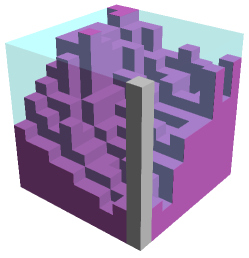
Figure 15. A configuration where loops affect the boundary condition: $\varphi$ is the completely filled cube represented with transparent light blue and $h$ is the solid configuration. Note that the presence of the gray “tower” in $h$ means that $\varphi$ is the only tiling satisfying the boundary condition so in order to have a non-trivial output in the algorithm we need to discard that tower. To the left of the gray tower, another one reaches the height of $\varphi$ creating a hole in the domain $S$ which would also be removed in this example but could be preserved in $h_{1}$ if its area was large enough compared to its height.

As mentioned above, we can safely ignore any loop that does not surround a hole or touch the boundary and enumerate over them at the end so w.l.o.g. we assume that all loops touch a boundary. For each loop $\varrho$, we let $a(\varrho)$ be the area of $\varrho$ and $H(\varrho)$ be the total length of all loops inside $\varrho$, including $\varrho$ itself. To select which loop to keep, we proceed inductively starting from the innermost ones (the nesting of loops defines a natural partial order) and erasing $\varrho$ together with all the loops inside of it if $H(\varrho)\geq\varepsilon^{1/3}a(\varrho)$ (updating the values of $H$ as we erase loops). We let $S^{\prime}$ be the union of $S$ and the interior and support of all erased loops and we will construct a tiling of $S^{\prime}$.

We first apply the above construction ignoring all the loops, let $h_{0}$ be the corresponding SOS height function and $\psi_{0}$ be the tiling constructed in this way. If $h_{0}$ is already in the set of “bad” configurations ${\mathcal{H}}^{\prime}$, then we simply enumerate over the remaining loops and declare $h$ to also be in ${\mathcal{H}}^{\prime}$. Otherwise, we proceed as follows. First, note that any loop in $h$ must be either completely above or completely below $h_{0}$, since the level lines of $h_{0}$ do not cross the loops. We will first treat all the loops above $h_{0}$, and then do the same for the ones below, but from now on we focus on the first step. Let $h_{1}$ be the configuration obtained by adding all these loops to $h_{0}$ and let $\psi_{1}$ be the lowest tiling satisfying the boundary condition imposed by $h_{1}$ and with $\psi_{1}\geq\psi_{0}$.

We sort the innermost loops $\varrho_{i}$ by the value of $h_{1}$ inside of them and breaking ties arbitrarily. Next, let $\psi_{1}^{(i)}$ be defined inductively by enforcing the constraint $\psi_{1}^{(i)}=h_{1}$ on the intersection of $\partial S^{\prime}$ and the interior of $\varrho_{1},\ldots,\varrho_{i}$, i.e., the lowest tiling larger than $\psi_{0}$ and satisfying these constraints. The $\psi_{1}^{(i)}$’s form an increasing sequence of tilings and we let $A_{i}$ be the number of horizontal tiles which differ between $\psi_{1}^{(i-1)}$ and $\psi_{1}^{(i)}$.

Claim 5.18.

We have $\sum_{i}A_{i}\leq s$.

Proof.

By construction, $\psi^{(i)}_{1}$ is obtained from $\psi^{(i-1)}_{1}$ by setting $\psi^{(i)}_{1}=h(\varrho_{i})$ for some $x\in{\mathcal{P}}_{001}$ where we had $\psi^{(i)}_{1}<h(\varrho_{i})$. Since the $h(\varrho_{i})$ are non-increasing, each $x$ can appear in at most one $A_{i}$. ∎

We then enforce the constraints associated to all the other loops to get $\psi_{1}$. Let us turn to the enumeration of the number of tilings $\psi_{0}$ that could be turned into a given $\psi_{1}$ by taking into account the loops as above. We do the enumeration level by level. In each level, for each loop $\zeta$ we choose an innermost loop $\varrho_{i(\zeta)}$ contained in it (or $i(\zeta)=i$ if $\zeta=\varrho_{i}$ is already an innermost loop) and we extend the order between the $\varrho_{i}$ to that level. We index the loops by $\zeta_{k}$ in that order and we let $\Gamma_{k}$ be the level line after taking into account the constraints up to $\zeta_{k}$. In the same spirit as the $A_{i}$, we define lengths $L_{k}$ as the number of steps which moved for the first time between $\Gamma_{k-1}$ and $\Gamma_{k}$.

Figure 16. A schematic representation of the proof of Claim 5.19. The original path is represented with green/black/cyan colors depending on the division in the proof and the final path is represented in purple below both the blue loop $\zeta$ and the red loop $\varrho_{i(\zeta)}$. The area in orange is bounded by $A_{i}$, the area between the loop $\varrho$ and its corresponding level line (not represented in the picture) which must stay north of the green/black/cyan path.

Claim 5.19.

Let $\zeta=\zeta_{k}$ be a loop. There exists a universal constant $C>0$ such that the number of paths $\Gamma_{k-1}$ compatible with a given $\Gamma_{k}$ is at most

$$A_{i}^{3}e^{2C\sqrt{A_{i(\zeta)}}}2^{\operatorname{diam}(\varrho_{i(\zeta)})}\binom{L_{k}}{2|\zeta|}\,.$$

Proof.

We enumerate separately the different parts as in Fig. 16. Draw a SE to NW half line starting at the SW-most point of the loop $\zeta$; note that $\Gamma_{k}$ cannot cross this line but we can assume $\Gamma_{k-1}$ does (otherwise there is nothing to prove on the W side). Also draw a parallel line from the SW-most point of $\varrho_{i(\zeta)}$ and a straight N one and then copy with symmetric directions on the E side. We enumerate from the center outward. For the inner portion (cyan in Fig. 16) between the two vertical lines, we note that its length is at most $\operatorname{diam}(\varrho_{i(\zeta)})$, with $2$ choices per step and at most $A$ allowed vertical translations. Then the two paths in “$\frac{1}{8}$-plane” portions (the black paths in Fig. 16), we note that given the two areas between them, there are fewer of them than integer partitions with these twice these areas (which would correspond to paths in quarter planes). It is then standard that the number of partitions of an integer $n$ can be bounded by $e^{Cn}$ for some $C$. Finally for the paths between the parallel diagonal lines (green in Fig. 16), note that they are completely determined once we know their length and the positions of respectively the NE and SE steps for the W and E side. Then number of such steps is at most $|\zeta|$ because by construction $\zeta$ contains the loop $\varrho_{i(\zeta)}$ but also the total number of unknown steps at that point is at most $L_{i}$. ∎

Overall, bounding again a product of binomial coefficient by a single one and the sum of the $L_{k}$ by $s$, we find that the total number of ways to obtain a given $\psi_{1}$ is at most

$$\exp(2C\sum_{i}\sqrt{A_{i}}n_{i})2^{\sum_{i}\operatorname{diam}(\zeta_{i})n_{i}}\binom{s}{2\varepsilon s}$$

where $n_{i}$ is the number of loops $\zeta$ with $i(\zeta)=i$ (we absorbed the power of $A$ into $C$). Also for each $\zeta$, we must have $\operatorname{diam}(\zeta_{i})\leq|\zeta|$ so the second term is bounded by $2^{\varepsilon s}$.

Finally, we can use the preprocessing step to bound the sizes of the loops. Fix $i$ and denote by $\zeta_{1},\ldots,\zeta_{n_{i}}$ all the loops counted in $n_{i}$ from the innermost one, $\zeta_{1}=\varrho_{i}$, to the outermost one. Since $a(\zeta_{n})\leq|\zeta_{n}|^{2}$ and $H(\zeta_{n})\geq\sum_{m=1}^{n}|\zeta_{m}|$ for all $n$, we see that every loop must have a size at least $\varepsilon^{-1/3}$ and more generally that their length must satisfy the recursive inequality

$$|\zeta_{n+1}|(|\zeta_{n+1}|-\varepsilon^{-1/3})\geq\varepsilon^{-1/3}\sum_{m=1}^{n}|\zeta_{m}|.$$

It is straightforward to verify that this implies

$$|\zeta_{n}|\geq\tfrac{1}{3}\varepsilon^{-1/3}n$$

for all $n$, from which we get

$$\sum_{i}n_{i}^{2}\leq 2\varepsilon^{1/3}\sum_{\zeta}|\zeta|\leq 2\varepsilon^{4/3}s.$$

A simple Cauchy–Schwarz then proves (running the whole argument in the new configuration a second time to account for the presence of loops below $h$):

Claim 5.20.

For a given $\psi_{1}$, there are at most $\exp(C\varepsilon^{2/3}s)$ ways to choose $\psi_{0}$.

To conclude the proof of Proposition 5.1, we simply redo the enumeration of the possible paths $\Gamma_{h}$ taking into account Claim 5.20. Indeed, note that the points (1) to (7) are still valid to enumerate the excursions away from $\Gamma_{\psi_{0}}$, the initial configuration where we ignored all the loops and that what remain to enumerate are the steps where $\Gamma_{h}$ and $\Gamma_{\psi_{0}}$ agree. The number of steps where in addition $\psi_{0}$ agrees with $\psi_{1}$ (which is the actual output of the algorithm) is bounded by $g$ as in the case with no loops and accounts for at most $2^{g}$ choices. It remains to choose the steps where $\Gamma_{\psi_{0}}$ and $\Gamma_{h}$ agree but not with $\Gamma_{\psi_{1}}$, which we over-count by sampling all the parts of $\psi_{0}$ where it differs from $\psi_{1}$ using Claim 5.20. ∎

5.2. Application for bubble groups

Proposition 5.1 will provide us with a crucial estimate on $\beta H_{h}(\mathfrak{B})-\alpha G_{h,\varphi}^{\textup{{g}}}(\mathfrak{B})$ for a “typical” bubble group $\mathfrak{B}$. Recall from Eq. 4.15 that for every bubble group $\mathfrak{B}=(\{\mathsf{B}_{i}\},\{{\mathcal{C}}_{j}\})$ we have $|\Upsilon(\mathfrak{B})|\leq 5\sum_{i}|\mathsf{B}_{i}|$.

Lemma 5.21.

There exist an absolute constant $C>0$ such that, for every $\varphi$, $\varepsilon>0$ and $s>C$, there are at most $\exp(C\varepsilon^{1/4}s)$ bubble groups $\mathfrak{B}$ of size $|\Upsilon(\mathfrak{B})|=s$ and containing a fixed point $o$ so that

$$\beta H_{h}(\mathfrak{B})-\alpha G^{\textup{{g}}}_{h,\varphi}(\mathfrak{B})\leq\varepsilon^{1/3}(\alpha\varepsilon^{1/3}\wedge\beta\varepsilon)s\,.$$ (5.1)

Moreover, if $\varepsilon\leq\frac{1}{150}$ then for all such $\mathfrak{B}$, we have $\mathsf{V}_{1}(\mathfrak{B})\geq s/16$ for the potential $\mathsf{V}_{1}$ from Eq. 1.4, as well as $\beta H_{h}(\mathfrak{B})+\lambda\mathsf{V}(\mathfrak{B})\geq\beta-\lambda+\lambda s/(16\mathsf{M}_{0})$ for the general potential $\mathsf{V}$ from Definition 1.3.

Proof.

First observe that $H_{h}$ is additive on the bubbles $\mathsf{B}_{i}$ by its definition in Eq. 4.14. As for $G_{h,\varphi}^{\textup{{g}}}$, since the set $S^{\prime}$ in Proposition 5.1 is larger than just the bubble, we can unfortunately not directly sum the bound. Let $\psi_{i}$ be the tilings of the set $S^{\prime}_{i}$ obtained by applying Proposition 5.1 to the bubble $\mathsf{B}_{i}$, setting by convention $\psi_{i}=\varphi\mathord{\upharpoonright}_{S}$ for the cases where $h\in{\mathcal{H}}^{\prime}$. Each tile in some $\psi_{i}\cap h$ can have one of three possible orientation (i.e., it can belong to a translate of the ${\mathcal{P}}_{100},{\mathcal{P}}_{010}$ or ${\mathcal{P}}_{001}$ direction) to one type must account for at least $1/3$ of the total. Suppose by symmetry (in this proof, we will not consider $h$ as anything but an arbitrary set of faces) that it is the ${\mathcal{P}}_{100}$ direction. We can view each tiling as a monotone function over a $\mathbb{Z}^{2}$ tiling of the ${\mathcal{P}}_{100}$ plane exactly as we often do over the ${\mathcal{P}}_{001}$ plane and similarly to the above we can assume that for at least half of these faces satisfy $\psi_{i}(u)\geq\varphi(u)$. We let

$$\psi=\max(\{\psi_{i}\}\cup\{\varphi\})$$

in that representation, i.e., for any face $u$ of ${\mathcal{P}}_{100}$, $\psi(u)$ is the maximum of all $\varphi(u)$ and of all the $\psi_{i}(u)$ that are well defined. Clearly, $\psi$ is well defined as an integer function but we need to check its monotonicity to show that it is indeed a tiling. For this, fix some $u$ and let $u^{\prime}$ be one of its neighbor with $u^{\prime}\geq u$. Suppose first that $i,i^{\prime}$ are such that $\psi_{i}(u)=\psi(u)$ and $\psi_{i^{\prime}}(u^{\prime})=\psi(u^{\prime})$, if $\psi_{i^{\prime}}$ is defined at $u$, then the proof is trivial so we can assume that it is not the case. Since $\psi_{i^{\prime}}$ is not defined at $u$ but is compatible with $\varphi$ outside of its domain of definition, one must have $\psi_{i^{\prime}}(u^{\prime})\leq\varphi(u)$ but by assumption $\varphi(u)\leq\psi_{i}(u)$. The proof is similar if $\psi(u)=\varphi(u)$ or $\psi(u^{\prime})=\varphi(u^{\prime})$. We also note that, since for each $i$, $|S^{\prime}_{i}\setminus S_{i}|\leq\varepsilon^{2/3}|S_{i}|$, going from the $\psi_{i}$ to $\psi$ misses at most $\varepsilon^{2/3}\sum_{|\Upsilon_{111}(\mathfrak{B}_{i})|}$ faces. Overall we get

$$\sum_{i}|\psi\cap h\cap\Upsilon_{111}^{-1}(S_{i})|\geq\frac{1}{6}\sum_{i}|\psi_{i}\cap h|-2\varepsilon^{2/3}\sum_{i}|S_{i}|.$$

Since the $S_{i}^{\prime}\setminus S_{i}$ also contain all the faces where $\varphi$ and $h$ agree but not $\psi$, we then get

$$G^{\textup{{g}}}_{h,\varphi}(\mathfrak{B})\leq G^{\textup{{g}}}_{h,\varphi}(\psi)\leq-\frac{1}{6}\sum_{i}|\psi_{i}\cap h|+2\varepsilon^{2/3}\sum_{i}|S_{i}|\,.$$ (5.2)

Consider $\psi$ constructed in this manner, and call a $\mathsf{B}_{i}$ bad if the corresponding SOS height function $h$ belongs to the exceptional subset ${\mathcal{H}}^{\prime}$ from Proposition 5.1, with the same choice of $\varepsilon$ as we have here, and good otherwise.

We will enumerate bubble groups with $\beta H_{h}(\mathfrak{B})-\alpha G^{\textup{{g}}}_{h,\varphi}(\mathfrak{B})\leq\varepsilon^{1/3}(\alpha\varepsilon^{1/3}\wedge\beta\varepsilon)$ using the above bound on $G^{\textup{{g}}}$. Observe that we may assume

$$\sum_{i}|\mathsf{B}_{i}|\mathbbm{1}_{\{\mathsf{B}_{i}\text{ is {\tt good}}\}}\leq 24\varepsilon^{1/3}s\,,$$ (5.3)

since every good bubble $\mathsf{B}_{i}$ has either $H_{h}(\mathsf{B}_{i})\geq\varepsilon|\mathsf{B}|$ or $|\psi_{i}\cap h|\geq\varepsilon^{1/3}|\mathsf{B}|$ (recall $h\cap\varphi=\emptyset$ on an $(h,\varphi)$-bubble), so every such $\mathsf{B}$ contributes at least $(\alpha\varepsilon^{1/3}\wedge\beta\varepsilon)|\mathsf{B}|$ to $\beta H_{h}(\mathfrak{B})-\alpha G^{\textup{{g}}}_{h,\varphi}(\mathfrak{B})$, with Eq. 5.2 in mind for the contribution to $G_{h,\varphi}^{\textup{{g}}}(\mathfrak{B})$.

To control the contribution of bad bubbles, first observe the following.

Fact 5.22.

Let $\mathsf{B}_{i}$ be an $(h,\varphi)$-bubble. If $\mathsf{B}_{i}$ is bad as defined above then $|\mathsf{B}_{i}|>1/\varepsilon$.

Proof.

For $\mathsf{B}_{i}$ to belong to ${\mathcal{H}}^{\prime}$ as per Proposition 5.1, necessarily $|h\cap\mathsf{B}_{i}|>|\varphi\cap\mathsf{B}_{i}|$, as otherwise $h\cap\mathsf{B}_{i}$ is itself a tiling whence $|h\cap\psi_{i}|=|\mathsf{B}_{i}|/2>\varepsilon^{1/3}|\mathsf{B}_{i}|$ (by taking $\psi_{i}=h\cap\mathsf{B}_{i}$), so $\mathsf{B}_{i}$ is good. Since we must also have $H<\varepsilon|\mathsf{B}_{i}|$ from the criteria of ${\mathcal{H}}^{\prime}$, we deduce that $|\mathsf{B}_{i}|>1/\varepsilon$. ∎

We will also need the following simple deterministic observation.

Fact 5.23.

For any $\varepsilon>0$ and connected set $S$ of faces of the triangular lattice ${\mathcal{T}}$, the number of faces of $\lceil\varepsilon^{-1}\rceil\mathbb{T}$ intersecting $S$ is at most $12\lceil\varepsilon|S|\rceil$.

Proof.

Let $\mathbb{T}^{\prime}$ be the sub-lattice of $\mathbb{T}$ made of tiles with side-length $\lceil 1/\varepsilon\rceil$, and let $T$ be the number of tiles of $\mathbb{T}^{\prime}$ that intersect $S$. The faces of the triangular lattice $\mathbb{T}$ can be colored using 6 colors such that two faces with the same color share neither an edge nor a vertex. Select the single-color sub-lattice containing the most faces of $\mathbb{T}^{\prime}$ which intersect $S$ and let $T^{\prime}$ be number of tiles in this set. If $T^{\prime}>1$, since $S$ is connected, we can associate to each of these tiles a path in $S$ of length $1/(2\varepsilon)$ connecting $S\cap t$ up to distance $1/(2\varepsilon)$ of $t$. Also of course $T^{\prime}\geq T/6$. Overall, we see that if $T>6$, then $|S|\geq|T|/(12\varepsilon)$ and in particular $T\leq 12\lceil\varepsilon S\rceil$. ∎

We can now start to enumerate our bubble groups. First we choose a connected set of $12\varepsilon s$ faces of $\lceil\varepsilon^{-1}\rceil\mathbb{T}$ and there are $C_{0}^{12\varepsilon s}$ ways to do it, with $C_{0}$ the growth constant for animals in the triangular lattice $\mathbb{T}$. The total area of this set in $\mathbb{T}$ is thus at most $12s/\varepsilon$. Then we choose the centers of all the bad bubbles: there are $\kappa\leq\varepsilon s$ of them because of 5.22 so there are less than $\sum_{\kappa}\binom{12s/\varepsilon}{\kappa}\leq\exp(C\varepsilon s\log(1/\varepsilon))$ possible choices at this step. Similarly, using Eq. 5.3, we can choose the area covered by good bubbles and an SOS configuration for each of them with at most $\binom{12s/\varepsilon}{\varepsilon^{1/3}s}C^{\varepsilon^{1/3}s}$ choices in total. Finally we choose the bad bubbles given their centers and by Proposition 5.1 there are only $\exp(c\varepsilon^{1/3}s)$ possible choices for those in total. Overall, the number of bubble groups we enumerated over is at most

$$c_{0}^{12\varepsilon s}\exp(2C\varepsilon^{1/3}s\log(1/\varepsilon))C^{\varepsilon^{1/3}s}\exp(c\varepsilon^{1/3}s)\leq\exp(C^{\prime}\varepsilon^{1/4}s)\,;$$

thus, at most $\exp[c\varepsilon^{1/4}s]$ bubble groups $\mathfrak{B}$ have $\beta H_{h}(\mathfrak{B})-\alpha G^{\textup{{g}}}_{h,\varphi}(\mathfrak{B})\leq\varepsilon^{1/3}(\alpha\varepsilon^{1/3}\wedge\beta\varepsilon)s$ (our criterion as per Eq. 5.1 for an exceptional bubble group $\mathfrak{B}$), as required.

It now remains to address the exceptional bubble groups $\mathfrak{B}$ via the potential $\mathsf{V}(\mathfrak{B})$. First let us consider $\mathsf{V}_{1}$ from Eq. 1.4; we recall Eq. 4.16 to find that

$$\mathsf{V}_{1}(\mathfrak{B}) =G^{\textup{{g}}}_{h,\varphi}(\mathfrak{B})+\sum_{\mathsf{B}\in\mathfrak{B}}|\varphi\cap\mathsf{B}|=G^{\textup{{g}}}_{h,\varphi}(\mathfrak{B})+\sum_{\mathsf{B}\in\mathfrak{B}}(|\mathsf{B}|-H_{h}(\mathsf{B}))/2$$

$$\geq-\frac{\beta H_{h}(\mathfrak{B})-\alpha G^{\textup{{g}}}_{\varphi,h}(\mathfrak{B})}{\alpha\wedge\beta}+\frac{1}{10}|\Upsilon(\mathfrak{B})|\,,$$

where we used Eq. 3.3 in the first line and Eq. 4.15 in the second one. The numerator in the first term is (by definition) at most $\varepsilon^{2/3}(\alpha\wedge\beta)|\Upsilon(\mathfrak{B})|$ for every $\mathfrak{B}$ which fails to satisfy Eq. 5.1. For every $\varepsilon\leq\frac{1}{150}$, we thus have $\mathsf{V}_{1}(\mathfrak{B})\geq(-\frac{1}{28}+\frac{1}{10})|\Upsilon(\mathfrak{B})|>\frac{1}{16}|\Upsilon(\mathfrak{B})|$, as required.

For the general family of $\mathsf{V}$, let $\{S_{i}\}_{i=1}^{m}$ (for some $m\geq 1$) be the connected components of $\psi^{\sqcup}\setminus h$. Recall from Definition 1.3 that $\mathsf{V}$ collects at least $\lfloor|S_{i}|/\mathsf{M}_{0}\rfloor>|S_{i}|/\mathsf{M}_{0}-1$ faces of each $S_{i}$ (whereas $\mathsf{V}_{1}$ collected all faces of these components), so that, in light of our lower bound on $\mathsf{V}_{1}(\mathfrak{B})$,

$$\mathsf{V}(\mathfrak{B})\geq\frac{\mathsf{V}_{1}(\mathfrak{B})}{\mathsf{M}_{0}}-m>\frac{|\Upsilon(\mathfrak{B})|}{16\mathsf{M}_{0}}-m\,;$$

Since $\psi^{\sqcup}$ maximizes $|h\cap\psi|$ over all tilings $\psi$, for each $i$ it must be that $h\mathord{\upharpoonright}_{\Upsilon(S_{i})}$ is not a tiling (or else we could replace $\psi^{\sqcup}$ by that tiling in $S_{i}$ and strictly increase its intersection with $h$). In particular, one has $H_{h}(\mathfrak{B})\geq m$, as $h$ has at least one excess face per each of the components $S_{i}$. Combining these bounds gives $\beta H_{h}(\mathfrak{B})+\lambda\mathsf{V}(\mathfrak{B})\geq(\beta-\lambda)m+\lambda|\Upsilon(\mathfrak{B})|/(16\mathsf{M}_{0})$, completing the proof. ∎

Towards an application for the dynamics that will appear in the proof of Theorem 6.1, we need an analogous statement for pairs $(S,\{\mathfrak{B}_{i}\})$ where $S$ is a connected set of faces of $\lceil\frac{1}{\gamma}\rceil\mathbb{T}$ that intersects each of the bubble groups in $\{\mathfrak{B}_{i}\}$.

Lemma 5.24.

There exists an absolute constant $C>0$ such that the following holds for every $\varphi$, $\varepsilon,\gamma>0$ and $s>C$. There are at most $\exp[C(\varepsilon^{1/4}+\gamma^{2})s]$ pairs $(S,\{\mathfrak{B}_{i}\})$, where $S$ is a connected set obtained as the union of triangles of $\lceil\frac{1}{\gamma}\rceil\mathbb{T}$ and $\{\mathfrak{B}_{i}\}$ is a collection of disjoint bubble groups such that $\Upsilon(\mathfrak{B}_{i})\cap S\neq\emptyset$ for all $i$, with $s=|S|\;\vee\;\sum_{i}|\Upsilon(\mathfrak{B}_{i})|$ and containing a fixed point $o$, so that

$$\sum_{i}\left(\beta H_{h}(\mathfrak{B}_{i})-\alpha G^{\textup{{g}}}_{h,\varphi}(\mathfrak{B}_{i})\right)\leq\varepsilon^{2/3}(\alpha\varepsilon^{1/3}\wedge\beta\varepsilon)\sum_{i}|\Upsilon(\mathfrak{B}_{i})|\,.$$

Furthermore, if $\varepsilon\leq\frac{1}{512}$ then for all such exceptional $(S,\{\mathfrak{B}_{i}\})$ we have

$$\sum_{i}\Big{(}\beta H_{h}(\mathfrak{B}_{i})+\lambda\mathsf{V}(\mathfrak{B}_{i})\Big{)}\geq\beta-\lambda+\frac{\lambda}{20\mathsf{M}_{0}}\sum_{i}|\Upsilon(\mathfrak{B}_{i})|\,.$$

Proof.

The proof is completely analogous to Lemma 5.21 so we only give a sketch. The total area of bubble groups that are good in the sense of Lemma 5.21 is at most $\varepsilon s$ while bad bubble groups in the sense of Lemma 5.21 provide very little entropy. The proof is then identical to Lemma 5.21 simply replacing bubbles by bubble groups, with the additional step of a final enumeration over $S$. It is there (using 5.23) where the $\exp[\gamma^{2}s]$ term appears.

For the final assertion, denote $\beta H_{h}(\mathfrak{B})-\alpha G^{\textup{{g}}}_{h,\varphi}(\mathfrak{B})$ by $f(\mathfrak{B})$ in this proof for brevity. Our assumption $\sum_{i}f(\mathfrak{B}_{i})\leq\varepsilon^{2/3}(\alpha\varepsilon^{1/3}\wedge\beta\varepsilon)s$ implies that

$$\sum_{i}|\Upsilon(\mathfrak{B}_{i})|\mathbbm{1}_{\{f(\mathfrak{B}_{i})<8\varepsilon^{2/3}(\alpha\varepsilon^{1/3}\wedge\beta\varepsilon)|\Upsilon(\mathfrak{B}_{i})|\}}>\tfrac{7}{8}s\,.$$

By Lemma 5.21, if $\varepsilon\leq\frac{1}{150}$ then $\beta H_{h}(\mathfrak{B})+\lambda\mathsf{V}(\mathfrak{B})\geq\beta-\lambda+\lambda|\Upsilon(\mathfrak{B}_{i})|/(16\mathsf{M}_{0})$ holds for every $\mathfrak{B}_{i}$ with $f(\mathfrak{B}_{i})\leq\varepsilon^{1/3}(\alpha\varepsilon^{1/3}\wedge\beta\varepsilon)|\Upsilon(\mathfrak{B}_{i})|$, thus for every $\mathfrak{B}_{i}$ that contributes to the above sum (as $\varepsilon\leq\frac{1}{512}$). So, the restriction of $\sum_{i}(\beta H_{h}(\mathfrak{B}_{i})+\lambda\mathsf{V}(\mathfrak{B}_{i}))$ to these $\mathfrak{B}_{i}$’s already suffices, as $\frac{1}{16}\cdot\frac{7}{8}s>s/20$. ∎

6. Local decomposition of $\pi_{\varphi,\hat{\beta}}$

Our goal in this section is to decompose $\int\pi_{\varphi,\hat{\beta}}(\cdot)\mathrm{d}\hat{\beta}$ as follows.

Theorem 6.1.

There is an absolute constant $C$ such that if $\lambda<\frac{1}{C}$ and $\alpha\wedge\beta>C\lambda^{20}$, then there exist functions $\mathfrak{g}^{\pi}_{r}$ for $r=2^{k}$ with $k=0,1,\ldots$, such that for every $N$,

$$\bigg{|}\int_{\beta}^{\infty}\pi_{\varphi,\hat{\beta}}(H_{h})\mathrm{d}\hat{\beta}-\sum_{x\in\mathbb{T}_{N}}\sum_{\begin{subarray}{c}0\leq r<N/2\\ r=2^{k}\end{subarray}}\mathfrak{g}^{\pi}_{r}(\varphi\mathord{\upharpoonright}_{B(x,r)})\bigg{|} \leq Ce^{-\beta-\frac{\lambda^{2}}{C\mathsf{M}_{0}}N}\,,$$ (6.1)

and for every integer $r=2^{k}$ ($k\geq 0$) one has $\|\mathfrak{g}_{r}^{\pi}\|_{\infty}\leq Ce^{-\beta-\frac{\lambda^{2}}{C\mathsf{M}_{0}}r}$.

Recalling the definition of $\pi_{\varphi,\hat{\beta}}$ from Eq. 2.12, thanks to Eq. 4.14 we have that

$$\pi_{\varphi,\hat{\beta}}(h)\propto\exp\bigg{[}\sum_{\begin{subarray}{c}\mathfrak{B}\,:\;\mathfrak{B}\text{ is an}\\ \text{$(h,\varphi)$-bubble group}\end{subarray}}\!\!\!\!\!\Big{[}-\hat{\beta}H(\mathfrak{B})+\alpha G^{\textup{{g}}}(\mathfrak{B})-\log Z_{\mu}^{\infty}(\mathfrak{B})-\lambda\mathsf{V}(\mathfrak{B})\Big{]}-\int_{\alpha}^{\infty}\mu_{h,\hat{\alpha}}(\overline{G}_{h})\mathrm{d}\hat{\alpha}\bigg{]}\,.$$ (6.2)

As was the case for the measures $\mu$ and $\nu$, we analyze the measure $\pi$ by defining an appropriate Gibbs sampler, and establishing that (a) it contracts w.r.t. an appropriate metric on SOS configurations, and therefore mixes rapidly; and (b) its speed of propagating information is uniformly bounded. As mentioned in Section 1.2.4, each of these tasks is significantly more challenging than the analogs for $\mu$ and $\nu$ because the effects of the term $\int\mu_{h,\hat{\alpha}}(\overline{G}_{h})\mathrm{d}\hat{\alpha}$ are hard to control.

More precisely, we will see (see, e.g., the proof of Proposition 6.10) that the SOS configuration at two different positions may interact strongly through this term when there exists a dense set of bubble groups connecting them. This introduces two difficulties: First, a large dense set comprised of small bubble groups $\{\mathfrak{B}_{i}\}$ will be a bottleneck for any “local” dynamics since in such a case the interaction through the integral might dominate the others terms for each individual $\mathfrak{B}_{i}$, stopping us from adding or removing them one by one. That is why the dynamics in Section 6.2 will be defined with possibly large single updates: it is designed to allow such a bottleneck to be removed in a single step. Second, at the technical level, we will need to measure the local density in our bounds on the integral, hence the notion of enclosure and fenced set defined below.

6.1. Bounds on the integral interaction.

Let $\rho$ denote the density of a set $S\subset\mathbb{T}$ with respect to an SOS configuration $h$:

$$\rho(S,h)=\frac{1}{|S|}\sum_{\mathfrak{B}\in h}|\Upsilon(\mathfrak{B})|\mathbbm{1}_{\{\Upsilon(\mathfrak{B})\cap S\neq\emptyset\}}\,.$$ (6.3)

Definition 6.2 (Enclosure).

Let $h$ be an SOS configuration and let $\mathfrak{B}_{0}$ be an $(h,\varphi)$-bubble group. An enclosure $R_{0}$ of $\mathfrak{B}_{0}$ with density $\rho_{0}$, which unless specified otherwise we take as $\rho_{0}=\frac{1}{10}$, is a connected set $R_{0}$ satisfying:

1. $R_{0}\supseteq\Upsilon(\mathfrak{B}_{0})$.

2. No $(h,\varphi)$-bubble group $\mathfrak{B}$ has $\Upsilon(\mathfrak{B})\cap\partial R_{0}\neq\emptyset$.

3. It has density (as per Eq. 6.3) at least $\rho_{0}$.

4. There is no set $R$ with $|R|>|R_{0}|$ that satisfies Items (1), (2) and (3).

Similarly, an enclosure of a set of bubble group $\{\mathfrak{B}^{0}_{i}\}$ is a set satisfying the above condition and such that each of its connected component contains at least on of the $\Upsilon(\mathfrak{B}^{0}_{i}\}$.

Remark 6.3.

Every bubble group $\mathfrak{B}_{0}$ has an enclosure $R_{0}$ as above: Indeed, $\Upsilon(\mathfrak{B}_{0})$ trivially satisfies Items (1) and (2) while Item (3) is given by Eq. 4.15; thus, the collection of sets $R$ satisfying Items (1), (2) and (3) is non-empty and any element of maximal size can be chosen as $R_{0}$. We emphasize that, typically, a bubble group will admit many different enclosures.

Definition 6.4 (Fenced set).

Let $h$ be an SOS configuration. A set $R$ is said to be fenced with density $\rho_{0}$, which unless specified otherwise we take as $\rho_{0}=\frac{1}{10}$, if no $(h,\varphi)$-bubble group $\mathfrak{B}$ has $\Upsilon(\mathfrak{B})\cap\partial R\neq\emptyset$ and if every connected set $S\subseteq\mathbb{T}_{N}\setminus R$ but with $\partial S\cap\partial R\neq\emptyset$ has $\rho(S,h)<\rho_{0}$.

Note that any enclosure is a fenced set but the converse is not true. Note also that being a fenced set is a decreasing condition on the set of bubble groups of $h$.

Our first step is to control the effect of adding or removing a set of bubble groups on $\int\mu_{h,\hat{\alpha}}(\overline{G}_{h})\mathrm{d}\hat{\alpha}$.

Proposition 6.5.

For all $\rho_{0}<\frac{1}{5}$, there exists $C$ such that the following holds. Let $\hat{h}$ be an SOS configuration, let $\{\mathfrak{B}_{i}\}$ be a collection of bubble groups of $\hat{h}$ and let $h$ be the configuration obtained by removing the $\mathfrak{B}_{i}$ from $\hat{h}$, i.e., $h=\hat{h}\vartriangle(\bigcup_{i}\bigcup_{\mathsf{B}\in\mathfrak{B}_{i}}\mathsf{B})$. If $R$ is a fenced set with density $\rho_{0}$ with respect to $\hat{h}$ (as per Definition 6.4) such that $\bigcup_{i}\Upsilon(\mathfrak{B}_{i})\subset R$, then

$$\Big{|}\int_{\alpha}^{\infty}\big{(}\mu_{\hat{h},\hat{\alpha}}(\overline{G}_{\hat{h}})-\mu_{h,\hat{\alpha}}(\overline{G}_{h})\big{)}\mathrm{d}\hat{\alpha}\Big{|}\leq C|R|\,.$$ (6.4)

Proof.

Note that for any $h$, denoting by $\{\mathsf{B}_{i}\}$ a consistent collection of $\phi\vartriangle\psi$ bubbles,

$$\log Z_{\mu}^{\alpha} \geq\log\big{(}\sum_{\{\mathsf{B}_{i}\}\subset R}e^{-\alpha\sum_{i}\overline{G}_{h}(\mathsf{B}_{i})}\big{)}+\log\big{(}\sum_{\{\mathsf{B}_{j}\}\subset R^{c}}e^{-\alpha\sum_{j}\overline{G}_{h}(\mathsf{B}_{j})}\big{)}$$

$$\log Z_{\mu}^{\alpha} \leq\log\big{(}\sum_{\{\mathsf{B}_{i}\}\subset R}e^{-\alpha\sum_{i}\overline{G}_{h}(\mathsf{B}_{i})}\big{)}+\log\big{(}\sum_{\{\mathsf{B}_{j}\}:\mathsf{B}_{j}\cap\partial R\neq\emptyset}e^{-\alpha\sum_{i}\overline{G}_{h}(\mathsf{B}_{j})}\big{)}+\log\big{(}\sum_{\{\mathsf{B}_{k}\}\subset R^{c}}e^{-\alpha\sum_{i}\overline{G}_{h}(\mathsf{B}_{k})}\big{)}$$

Indeed, since the compatibility condition between bubbles is just that they cannot intersect, the first inequality amounts to restricting the partition function to configuration $\psi$ with $\psi=\varphi$ on $\partial R$ and the second is over-counting by ignoring the compatibility condition between the three sets of bubbles. Applying Lemma 2.6 to all terms, we get

$$\int\mu_{\hat{\alpha}}(\overline{G}_{h}(R)|\psi=\varphi\text{ on }\partial R)+\log Z_{\mu}^{\infty}(R)+\int\mu_{\hat{\alpha}}(\overline{G}_{h}(R^{c})|\psi=\varphi\text{ on }\partial R)+\log Z_{\mu}^{\infty}(R^{c})\\ \leq\int\mu_{\hat{\alpha}}(\overline{G}_{h})+\log Z_{\mu}^{\infty}\leq\\ \int\mu_{\hat{\alpha}}(\overline{G}_{h}(R)|\psi=\varphi\text{ on }\partial R)+\log Z_{\mu}^{\infty}(R)+\int\mu_{\hat{\alpha}}(\overline{G}_{h}(R^{c})|\psi=\varphi\text{ on }\partial R)+\log Z_{\mu}^{\infty}(R^{c})\\ +\int\mu_{\partial R,\hat{\alpha}}(\overline{G}_{h}(\partial R))+\log Z_{\partial}^{\infty}.$$ (6.5)

Indeed, thanks to the fact that the energy $\overline{G}$ is zero-range, the measure obtained when applying Lemma 2.6 just to the partition function of configurations inside $R$ coincides with the conditional measure $\mu$ given $\psi=\psi\text{ on }\partial R$.

In the expression above, note further that since $\partial R$ does not intersect any bubble group, $\log Z_{\mu}^{\infty}=\log Z_{\mu}^{\infty}(R)+\log Z_{\mu}^{\infty}(R^{c})$ and $\log Z_{\partial}^{\infty}=0$. Also, the terms outside of $R$ are equal for $h$ and $\hat{h}$. Overall, we therefore have

$$\int\mu_{\hat{h},\hat{\alpha}}(\overline{G}_{\hat{h}}(R))-\int\mu_{h,\hat{\alpha}}(\overline{G}_{h}(R))-\int\mu_{h,\partial R}(\overline{G}_{h}(\partial R))\\ \leq\int\mu_{\hat{h}}-\int\mu_{h}\leq\\ \int\mu_{\hat{h}}(\overline{G}_{\hat{h}}(R))-\int\mu_{h}(\overline{G}_{h}(R))+\int\mu_{\hat{h},\partial R}(\overline{G}_{h}(\partial R))$$ (6.6)

and applying Lemma 2.6 in the opposite direction

$$\log Z_{\mu_{\hat{h}}}^{\alpha}(R)-\log Z_{\mu_{\hat{h}}}^{\infty}(R)-\log Z_{\mu_{h}}^{\alpha}(R)+\log Z_{\mu_{h}}^{\infty}(R)-\log Z_{\mu_{h,\partial}}^{\alpha}(\partial R)\\ \leq\int\mu_{\hat{h}}-\int\mu_{h}\leq\\ \log Z_{\mu_{\hat{h}}}^{\alpha}(R)-\log Z_{\mu_{\hat{h}}}^{\infty}(R)-\log Z_{\mu_{h}}^{\alpha}(R)+\log Z_{\mu_{h}}^{\infty}(R)+\log Z_{\mu_{\hat{h},\partial}}^{\alpha}(\partial R)\,.$$ (6.7)

All the $\log Z(R)$ aterms re bounded by $C_{0}|R|$ because they count tilings of $R$. The terms $\log Z(\partial R)$ are also bounded similarly because having a surface larger than $|R|$ outside of $R$ is exponentially costly (via $\overline{G}$) because we cannot be dense by definition of a fenced set. This yields Eq. 6.4. ∎

The above proposition will be useful to understand the dynamics close to a region of interest where we do not expect the true value of the interactions to be particularly small. The following bound will refine that bound in terms of a single enclosure $R_{0}$ and the sizes of the bubble groups as opposed to the more complicated fenced sets.

Lemma 6.6.

There exists a constant $C$ such that the following holds. Fix $h$ an SOS configuration, let $\mathfrak{B}^{0}$ be a bubble group that can be added to $h$ and let $h^{\prime}$ be the corresponding configuration. Let $R_{0}$ be an enclosure of $\mathfrak{B}^{0}$ in $h^{\prime}$. Further fix a set $\{\mathfrak{B}^{1}_{i}\}$ of bubble groups which can be added in both $h$ and $h^{\prime}$, denoting the resulting configurations by $\hat{h},\hat{h}^{\prime}$. Let $S$ be a connected set intersecting each $\Upsilon(\mathfrak{B}^{1}_{i})$. If $\operatorname{dist}(\bigcup_{i}\Upsilon(\mathfrak{B}_{i}),R_{0})\leq 40(|R_{0}|+\sum|\Upsilon(\mathfrak{B}_{i})|)$, then

$$\Big{|}\int_{\alpha}^{\infty}\big{(}\mu_{\hat{h}^{\prime},\hat{\alpha}}(\overline{G}_{\hat{h}^{\prime}})-\mu_{h^{\prime},\hat{\alpha}}(\overline{G}_{h^{\prime}})\big{)}\mathrm{d}\hat{\alpha}\Big{|}\leq C(|S|+\sum_{i}|\Upsilon(\mathfrak{B}_{i})|+|R_{0}|)\,,$$

and similarly for the pair $(h,\hat{h})$.

Proof.

Let $R_{1}$ be an enclosure for the $\mathfrak{B}^{1}_{i}$ in configuration $\hat{h}^{\prime}$ with density $\frac{3}{20}$. It is a fenced set in any of $h,h^{\prime},\hat{h},\hat{h}^{\prime}$ and therefore by Proposition 6.5 it is enough to bound its size.

Suppose by contradiction that $|R_{1}|\geq 200(|S|+\sum_{i}|\Upsilon(\mathfrak{B}_{i})|+|R_{0}|)$. Let $R^{\prime}$ be obtained as $(R_{1}\cup S)\setminus R_{0}$ to which we add a minimal path to $\partial R_{0}$ and a path on the outer boundary of $R_{0}$. Since each connected component of $R_{1}$ contains one of the $\Upsilon(\mathfrak{B}_{i}^{1})$ and $S$ intersects all of them, $R_{1}\cup S$ is connected and therefore $R^{\prime}$ must also be connected since any connection in $R_{1}\cup S$ going through $R_{0}$ can now go through the outer boundary path. By definition $\rho(R_{1},\hat{h}^{\prime})\geq\frac{3}{20}$ so

$$|R^{\prime}|\rho(R^{\prime},h)\geq|R_{1}|\frac{3}{20}-\sum_{i}|\Upsilon(\mathfrak{B}^{1}_{i})|-|R_{0}|\,,$$

while

$$|R^{\prime}| \leq|R_{1}|+|S|+\operatorname{dist}\Big{(}\bigcup\Upsilon(\mathfrak{B}_{i}^{1}),R_{0}\Big{)}+11|R_{0}|$$

$$\leq|R_{1}|+|S|+51|R_{0}|+40\sum|\Upsilon(\mathfrak{B}_{i}^{1})|\,.$$

Combining the two bound, we see that

$$\rho(R^{\prime},h) \geq\Big{(}\frac{3}{20}-\frac{\sum_{i}|\Upsilon(\mathfrak{B}^{1}_{i})|+|R_{0}|}{|R_{1}|}\Big{)}\Big{(}1-\frac{|S|}{|R_{1}|}-51\frac{\sum_{i}|\Upsilon(\mathfrak{B}^{1}_{i})|+|R_{0}|}{|R_{1}|}\Big{)}$$

$$\geq\frac{3}{20}-10\frac{\sum_{i}|\Upsilon(\mathfrak{B}^{1}_{i})|+|R_{0}|}{|R_{1}|}\geq\frac{1}{10}\,,$$

where the last inequality used that $|R_{1}|\geq 200\sum_{i}|\Upsilon(\mathfrak{B}_{i}^{1})|+|R_{0}|$. This is a contradiction with the fact that $R_{0}$ is an enclosure of $\mathfrak{B}_{0}$. ∎

We also need a statement controlling the interaction between far away bubble groups. The first step is to show a form of exponential decay in the measure $\mu_{h}$:

Proposition 6.7.

For all $\rho<\frac{1}{5}$, there exists $C_{0}$ such that the following holds for each $\hat{\alpha}$ large enough. Fix $h^{\prime}$ and an $(h^{\prime},\varphi)$-bubble group $\mathfrak{B}_{0}$, and let $h=h^{\prime}\vartriangle\bigcup_{\mathsf{B}\in\mathfrak{B}_{0}}\mathsf{B}$. Let $R^{\star}_{0}$ be a fenced set containing $\mathfrak{B}_{0}$ Then there is a coupling $\mu_{h,h^{\prime},\hat{\alpha}}$ of $\mu_{h,\hat{\alpha}},\mu_{h^{\prime},\hat{\alpha}}$ so that for all $f$,

$$\mu_{h,h^{\prime},\hat{\alpha}}(f\in\Upsilon(\psi\vartriangle\psi^{\prime}))\leq C_{0}e^{-\frac{1}{2}(\hat{\alpha}-C_{0})\operatorname{dist}(f,R_{0}^{\star})}\,.$$

Proof.

We define the coupling as follows. Sample the surfaces

$$\psi\sim\mu_{h,\hat{\alpha}}\qquad\mbox{and}\qquad\hat{\psi}\sim\mu_{h^{\prime},\hat{\alpha}}$$

independently, and let $A=\Upsilon(\psi\vartriangle\hat{\psi})$. Define the surface $\psi^{\prime}$ by

1. $\psi^{\prime}=\hat{\psi}$ on $R_{0}\setminus A$ and any connected component of $A$ touching $\partial R_{0}$;

2. $\psi^{\prime}=\psi$ on any other connected component of $A$.

By Lemma 4.5, we see that $\hat{\psi}$ and $\psi^{\prime}$ have the same law, and consequently $\mu_{h,h^{\prime},\hat{\alpha}}(f\in\Upsilon(\psi^{\prime}\vartriangle\psi))$ is bounded by the probability that there exists a connected component of $A$ connecting $f$ to $\partial R_{0}^{\star}$. (Note that the zero-range interactions of $\mu$ are crucial to making this switching legal.) Consider the part of this component outside of $R_{0}^{\star}$; it cannot be denser than $\frac{1-\varepsilon}{5}$ because of Item (4) so the probability that at least $\frac{1}{2}$ of it is covered by bubbles in either $\varphi\vartriangle\psi$ or $\varphi\vartriangle\hat{\psi}$ is bounded by $C_{0}e^{-\frac{1}{2}(\hat{\alpha}-C_{0})\operatorname{dist}(f,R_{0}^{\star})}$, with the constant $C_{0}$ accounting for an enumeration over all possible sets of bubbles (via a Peierls argument, done for $\psi$ under $\mu_{h,\hat{\alpha}}$ and separately for $\hat{\psi}$ under $\mu_{h^{\prime},\hat{\alpha}}$). ∎

We can now control the interaction between two far away bubble groups via the following.

Lemma 6.8.

For all $\rho<\frac{1}{5}$, there exists $C$ such that the following holds for every $\alpha$ large enough. Let $h$ be an SOS configuration and let $\mathfrak{B}^{0},\mathfrak{B}^{1}$ be two bubble groups that do not intersect and which can both be added to $h$. As before, let

$$h^{\prime}=h\vartriangle\bigcup_{\mathsf{B}\in\mathfrak{B}^{0}}\mathsf{B}\quad,\quad\hat{h}^{\prime}=h\vartriangle\bigcup_{\mathsf{B}\in\mathfrak{B}^{0}\cup\mathfrak{B}^{1}}\mathsf{B}\quad,\quad\hat{h}=h\vartriangle\bigcup_{\mathsf{B}\in\mathfrak{B}_{1}}\mathsf{B}\,.$$

Let $\hat{R}^{0},\hat{R}^{1}$ be enclosures with density $\rho$ of $\mathfrak{B}^{0}$ and $\mathfrak{B}^{1}$ w.r.t. $\hat{h}^{\prime}$ as per Definition 6.2. Then

$$\bigg{|}\int_{\alpha}^{\infty}\Big{(}\mu_{\hat{h}^{\prime},\hat{\alpha}}(\overline{G}_{\hat{h}^{\prime}})-\mu_{h^{\prime},\hat{\alpha}}(\overline{G}_{h^{\prime}})-\mu_{\hat{h},\hat{\alpha}}(\overline{G}_{\hat{h}})+\mu_{h,\hat{\alpha}}(\overline{G}_{h})\Big{)}\mathrm{d}\hat{\alpha}\bigg{|}\leq C(|\hat{R}_{0}|\wedge|\hat{R}_{1}|)e^{-\alpha\operatorname{dist}(\hat{R}_{0},\hat{R}_{1})/C}\,.$$

Moreover, if $(\mathfrak{B}^{0}_{i})_{1\leq i\leq m_{0}}$ and $(\mathfrak{B}^{1}_{i})_{1\leq i\leq m_{1}}$ are two family of bubble groups that can be simultaneously added (together) to $h$, then

$$\bigg{|}\int_{\alpha}^{\infty}\Big{(}\mu_{\hat{h}^{\prime},\hat{\alpha}}(\overline{G}_{\hat{h}^{\prime}})-\mu_{h^{\prime},\hat{\alpha}}(\overline{G}_{h^{\prime}})-\mu_{\hat{h},\hat{\alpha}}(\overline{G}_{\hat{h}})+\mu_{h,\hat{\alpha}}(\overline{G}_{h})\Big{)}\mathrm{d}\hat{\alpha}\bigg{|}\leq C_{0}\sum_{i,j}(|\hat{R}^{0}_{i}|\wedge|\hat{R}^{1}_{j}|)e^{-\alpha\operatorname{dist}(\hat{R}^{0}_{i},\hat{R}^{1}_{j})/C_{0}}\,,$$

where the $\hat{R}^{0}_{i}$, $\hat{R}^{1}_{j}$ are enclosures of the $\mathfrak{B}^{0}_{i}$ and $\mathfrak{B}^{1}_{j}$ respectively.

Proof.

We start with the first case involving only two bubble groups. The general idea is prove this result via an application of Proposition 6.7, creating a separate coupling for each face $f\in\mathbb{T}_{N}$ that would show that $f$ has an exponentially small contribution, as it cannot be close simultaneously to $\hat{R}_{0}$ and $\hat{R}_{1}$.

Since the condition on $R_{0}^{\star}$ from Proposition 6.7 is monotone on the set of bubble groups, we can apply Proposition 6.7 to both the pair $(h,h^{\prime})$ and $(\hat{h},\hat{h}^{\prime})$ using the same set $\hat{R}_{0}$. For the same reason, if we add $\mathfrak{B}_{1}$, we can still use Proposition 6.7 using $\hat{R}_{1}$. Overall, we see that we can define couplings such that

$$\mu_{h,h^{\prime},\hat{\alpha}}(f\in\Upsilon(\psi\vartriangle\psi^{\prime})) \leq C_{0}\,e^{-\frac{1}{2}(\hat{\alpha}-C_{0})\,\operatorname{dist}(f,\hat{R}_{0})}\,,$$

$$\mu_{\hat{h},\hat{h}^{\prime},\hat{\alpha}}(f\in\Upsilon(\hat{\psi}\vartriangle\hat{\psi}^{\prime})) \leq C_{0}\,e^{-\frac{1}{2}(\hat{\alpha}-C_{0})\operatorname{dist}(f,\hat{R}_{0})}\,,$$

$$\mu_{h,\hat{h},\hat{\alpha}}(f\in\Upsilon(\psi\vartriangle\hat{\psi})) \leq C_{0}\,e^{-\frac{1}{2}(\hat{\alpha}-C_{0})\operatorname{dist}(f,\hat{R}_{1})}\,,$$

$$\mu_{h^{\prime},\hat{h}^{\prime},\hat{\alpha}}(f\in\Upsilon(\psi^{\prime}\vartriangle\hat{\psi}^{\prime})) \leq C_{0}\,e^{-\frac{1}{2}(\hat{\alpha}-C_{0})\operatorname{dist}(f,\hat{R}_{1})}\,.$$

Now, we can decompose the integral over the contribution of each faces $x$ of $\mathbb{T}_{N}$. Let

$$\overline{G}_{h}^{x}(\psi)=\sum_{f\in\Upsilon^{-1}(x)}\overline{g}_{h}(f)\mathbbm{1}_{\{f\in\psi\}}\,$$

using the decomposition of $\overline{G}_{h}$ from Lemma 4.5 (as usual, for brevity, in what follows we omit the parameter $\psi$ from $\overline{G}_{h}^{x}$, as well as the corresponding $\psi^{\prime},\hat{\psi},\hat{\psi}^{\prime}$ from $\overline{G}^{x}_{h^{\prime}},\overline{G}^{x}_{\hat{h}},\overline{G}^{x}_{\hat{h}^{\prime}}$, respectively). Then

$$\bigg{|}\int_{\alpha}^{\infty} \Big{(}\mu_{\hat{h}^{\prime},\hat{\alpha}}(\overline{G}_{\hat{h}^{\prime}})-\mu_{h^{\prime},\hat{\alpha}}(\overline{G}_{h^{\prime}})-\mu_{\hat{h},\hat{\alpha}}(\overline{G}_{\hat{h}})+\mu_{h,\hat{\alpha}}(\overline{G}_{h})\Big{)}\mathrm{d}\hat{\alpha}\bigg{|}$$

$$\leq\sum_{x\in\mathbb{T}_{N}}\bigg{|}\int_{\alpha}^{\infty}\Big{(}\mu_{\hat{h}^{\prime},\hat{\alpha}}(\overline{G}^{x}_{\hat{h}^{\prime}})-\mu_{h^{\prime},\hat{\alpha}}(\overline{G}^{x}_{h^{\prime}})-\mu_{\hat{h},\hat{\alpha}}(\overline{G}^{x}_{\hat{h}})+\mu_{h,\hat{\alpha}}(\overline{G}^{x}_{h})\Big{)}\mathrm{d}\hat{\alpha}\bigg{|}$$

$$\leq 2\sum_{x\in\mathbb{T}_{N}}\int_{\alpha}^{\infty}\min\Big{(}\mu_{h,h^{\prime},\hat{\alpha}}(x\in\Upsilon(\psi^{\prime}\vartriangle\psi))+\mu_{\hat{h},\hat{h}^{\prime},\hat{\alpha}}(x\in\Upsilon(\hat{\psi}^{\prime}\vartriangle\hat{\psi}))+2\mathbbm{1}_{\{x\in\Upsilon(\mathfrak{B}_{0})\}},\,$$

$$\qquad\qquad\qquad\quad\quad\;\;\;\mu_{h,\hat{h},\hat{\alpha}}(x\in\Upsilon(\psi\vartriangle\hat{\psi}))+\mu_{h^{\prime},\hat{h}^{\prime},\hat{\alpha}}(x\in\Upsilon(\hat{\psi}^{\prime}\vartriangle\psi^{\prime}))+2\mathbbm{1}_{\{x\in\Upsilon(\mathfrak{B}_{1})\}}\Big{)}\,\mathrm{d}\hat{\alpha}.$$

Indeed, for the last line, note that we can bound the contribution of a single $x$ using two possible pairings of the four terms and we are free to use the better one depending on $x$. Furthermore, when $x\notin\Upsilon(\mathfrak{B}_{0})$ then $\overline{G}_{h}^{x}=\overline{G}_{h^{\prime}}^{x}$, and we bound the difference in the expectation of this variable under the two measures $\mu_{h,\hat{\alpha}}$ and $\mu_{h^{\prime},\hat{\alpha}}$, recalling that $|\overline{G}^{x}_{h}|\leq 1$ always holds, via

$$\int_{\alpha}^{\infty}|\mu_{h^{\prime},\hat{\alpha}}(\overline{G}_{h^{\prime}}^{x})-\mu_{h,\hat{\alpha}}(\overline{G}_{h}^{x})|\mathrm{d}\hat{\alpha}\leq 2\int_{\alpha}^{\infty}\mu_{h,h^{\prime},\hat{\alpha}}(x\in\Upsilon(\psi\vartriangle\psi^{\prime}))\mathrm{d}\hat{\alpha}\,.$$

For $x\in\Upsilon(\mathfrak{B}_{0})$ we used the trivial upper bound $|\overline{G}_{h}^{x}|+|\overline{G}_{h^{\prime}}^{x}|\leq 2$. The bounds for the other terms are similar (replacing $\mathfrak{B}_{0}$ by $\mathfrak{B}_{1}$).

Plugging in the bounds on $\mu_{h,h^{\prime},\hat{\alpha}}$ and using the fact that the indicators $\mathbbm{1}_{\{x\in\Upsilon(\mathfrak{B}_{0})\}}$ and $\mathbbm{1}_{\{x\in\Upsilon(\mathfrak{B}_{1})\}}$ cannot hold simultaneously, we see that overall

$$\bigg{|}\int_{\alpha}^{\infty}\big{(}\mu_{\hat{h}^{\prime},\hat{\alpha}}(\overline{G}_{\hat{h}^{\prime}})-\mu_{h^{\prime},\hat{\alpha}}(\overline{G}_{h^{\prime}})-\mu_{\hat{h},\hat{\alpha}}(\overline{G}_{\hat{h}})+\mu_{h,\hat{\alpha}}(\overline{G}_{h})\big{)}\mathrm{d}\hat{\alpha}\bigg{|} \leq C_{0}\sum_{f\in\mathbb{T}_{N}}e^{-\alpha(\operatorname{dist}(f,\hat{R}_{0})\vee\operatorname{dist}(f,\hat{R}_{1}))/C_{0}}$$

$$\leq C_{0}(|\hat{R}_{0}|\wedge|\hat{R}_{1}|)e^{-\alpha\operatorname{dist}(\hat{R}_{0},\hat{R}_{1})/C_{0}}\,,$$

which concludes the proof of the first part. (To see the last inequality, suppose w.l.o.g. that $|\hat{R}_{0}|\leq|\hat{R}_{1}|$, and take $d=\operatorname{dist}(\hat{R}_{0},\hat{R}_{1})$. The set of all $f$ at distance at least $d/2$ from $\hat{R}_{0}$ contributes at most $C|\hat{R}_{0}|e^{-(\alpha/C_{0})d/2}$ by summability of the exponent; on the other hand, every other face $f$ must have distance at least $d/2$ from $\hat{R}_{1}$ and there are at most $C|\hat{R}_{0}|d^{2}$ such faces.)

For the case with multiple bubble groups, it follows directly from monotonicity of fenced sets in Proposition 6.7 and the observation that

$$\mu_{\hat{h}^{\prime},\hat{\alpha}}(\overline{G}_{\hat{h}^{\prime}})-\mu_{h^{\prime},\hat{\alpha}}(\overline{G}_{h^{\prime}})-\mu_{\hat{h},\hat{\alpha}}(\overline{G}_{\hat{h}})+\mu_{h,\hat{\alpha}}(\overline{G}_{h})\\ =\sum_{i,j}\mu_{h_{i+1,j+1},\hat{\alpha}}(\overline{G}_{h_{i+1,j+1}})-\mu_{h_{i+1,j},\hat{\alpha}}(\overline{G}_{h_{i+1,j}})-\mu_{h_{i,j+1},\hat{\alpha}}(\overline{G}_{h_{i,j+1}})+\mu_{h_{i,j},\hat{\alpha}}(\overline{G}_{h_{i,j}})\,,$$

with $h_{i,j}$ the configuration obtained by adding the bubble groups $\mathfrak{B}^{0}_{1},\ldots,\mathfrak{B}^{0}_{i}$ and $\mathfrak{B}^{1}_{1},\ldots,\mathfrak{B}^{1}_{j}$. ∎

As for the bound involving only a single difference, it will be useful to have a version involving simpler quantities that the $\hat{R}_{i}$ above.

Lemma 6.9.

Let $h$, $\mathfrak{B}_{0}$, $\mathfrak{B}_{1}$ be an SOS configuration and two bubble groups that can be added to it as above. Let $h^{\prime},\hat{h},\hat{h}^{\prime}$ be obtained by adding $\mathfrak{B}_{0}$, $\mathfrak{B}_{1}$ or both to $h$. If an enclosure $R_{0}$ of $\mathfrak{B}_{0}$ in the configuration $h^{\prime}$ satisfies

$$\mathfrak{d}:=\operatorname{dist}\left(\Upsilon(\mathfrak{B}_{1}),R_{0}\right)>40(|R_{0}|+|\Upsilon(\mathfrak{B}_{1})|)\,,$$

then, for an absolute constant $C_{0}$,

$$\bigg{|}\int_{\alpha}^{\infty}\Big{(}\mu_{\hat{h}^{\prime},\hat{\alpha}}(\overline{G}_{\hat{h}^{\prime}})-\mu_{h^{\prime},\hat{\alpha}}(\overline{G}_{h^{\prime}})-\mu_{\hat{h},\hat{\alpha}}(\overline{G}_{\hat{h}})+\mu_{h,\hat{\alpha}}(\overline{G}_{h})\Big{)}\mathrm{d}\hat{\alpha}\bigg{|}\leq C_{0}e^{-\\ \\ \alpha\mathfrak{d}/C_{0}}\,.$$

More generally, for two family of bubble groups $(\mathfrak{B}^{0}_{i})_{1\leq i\leq m_{0}}$ and $(\mathfrak{B}^{1}_{i})_{1\leq i\leq m_{1}}$, if there exists enclosures of the $R_{i}^{0}$ of the $\mathfrak{B}_{i}^{0}$ in $h^{\prime}$ such that for all $i$

$$\operatorname{dist}\Big{(}\bigcup_{j}\Upsilon(\mathfrak{B}^{1}_{j}),R^{0}_{i}\Big{)}>40\Big{(}|R^{0}_{i}|+\sum_{j}|\Upsilon(\mathfrak{B}^{1}_{j})|\Big{)}\,,$$

then

$$\bigg{|}\int_{\alpha}^{\infty}\Big{(}\mu_{\hat{h}^{\prime},\hat{\alpha}}(\overline{G}_{\hat{h}^{\prime}})-\mu_{h^{\prime},\hat{\alpha}}(\overline{G}_{h^{\prime}})-\mu_{\hat{h},\hat{\alpha}}(\overline{G}_{\hat{h}})+\mu_{h,\hat{\alpha}}(\overline{G}_{h})\Big{)}\mathrm{d}\hat{\alpha}\bigg{|}\leq C_{0}\sum_{i}e^{-\alpha\operatorname{dist}(R^{0}_{i},\bigcup_{j}\Upsilon(\mathfrak{B}^{1}_{j}))/C_{0}}\,.$$

Proof.

Again we start with the case involving only two bubble groups. Assume we have such an $R_{0}$. Let $\hat{R}_{0},\hat{R}_{1}$ be enclosures of $\mathfrak{B}_{0},\mathfrak{B}_{1}$ in $\hat{h}^{\prime}$ but with density $3/20$, Lemma 6.8 applies so what remains to do is to bound $\operatorname{dist}(\hat{R}_{0},\hat{R}_{0})$ and their sizes.

We first argue that

$$\operatorname{dist}(R_{0},\hat{R}_{1})\geq\mathfrak{d}/10\,.$$

Suppose by contradiction that $\operatorname{dist}(R_{0},\hat{R}_{1})\leq\mathfrak{d}/10$. Since $\operatorname{dist}(\Upsilon(\mathfrak{B}_{1}),R_{0})\geq\mathfrak{d}$, then necessarily $|\hat{R}_{1}|\geq\frac{9}{10}\mathfrak{d}\geq 36(|R_{0}|+|\Upsilon(\mathfrak{B}_{1})|)$. In particular, the bubble groups common in $h^{\prime}$ and $\hat{h}^{\prime}$ and outside of $R_{0}$ must already have a positive density:

$$\sum_{\begin{subarray}{c}\text{$(h^{\prime},\varphi)$-bubble group $\mathfrak{B}$}\\ \mathfrak{B}\neq\mathfrak{B}_{1}\end{subarray}}|\Upsilon(\mathfrak{B})|\mathbbm{1}_{\{\Upsilon(\mathfrak{B})\cap R_{0}=\emptyset\}}\geq(\tfrac{3}{20}-\tfrac{1}{36})|\hat{R}_{1}|\geq\tfrac{1}{9}|\hat{R}_{1}|\geq\tfrac{1}{10}(|\hat{R}_{1}|+\mathfrak{d}/10)\,,$$

again using for the last step that $\mathfrak{d}/10\leq\frac{1}{9}|\hat{R}_{1}|$. Consider the union of $\hat{R}_{1}$ and the shortest path connecting it to $R_{0}$: the above equation shows that it has density at least $1/10$ even in $h^{\prime}$, contradicting the definition of $R_{0}$ (Definition 6.2).

We have thus proved that no set of density (in $\hat{h}^{\prime}$) more than $3/20$ can intersect both $\Upsilon(\mathfrak{B}_{1})$ and $R_{0}$. In particular, $\hat{R}_{0}$ cannot intersect $\Upsilon(\mathfrak{B}_{1})$ and it must have the same density in $\hat{h}^{\prime}$ and $\hat{h}$ but it therefore can be chosen to be smaller than $R_{0}$. This comparison of $R_{0},\hat{R}_{0}$ now implies that

$$\operatorname{dist}\big{(}\hat{R}_{0},\hat{R}_{1}\big{)}\geq\mathfrak{d}/10\,,$$

and we conclude by simply plugging this bound in Lemma 6.8.

With multiple bubble groups, since the distance condition involves the sum of the sizes, the same argument as above first shows that for each $i,j$, $\operatorname{dist}(\hat{R}_{j}^{1},R_{i}^{0})\geq\operatorname{dist}(\Upsilon(\mathfrak{B}_{j}),R^{0}_{i})/10$. Again from this we can deduce that we can choose $\hat{R}_{i}^{0}\subset R_{i}^{0}$ for all $i$. Using the bound on the distance, we can absorb a factor $\sum_{j}|\Upsilon(\mathfrak{B}^{1}_{j})|$ into the exponential and this concludes the proof. ∎

Finally, since the integral is always positive and since only dense regions of bubble groups contribute significantly, intuitively one could hope that it could be monotone. This does not seem to be correct but one can still in a sense ignore its effect, at the cost of losing the $G^{\textup{{g}}}$ and $\log(Z_{\mu}^{\infty})$ terms.

Proposition 6.10.

Let $\varphi$ be a tiling of $\mathbb{T}_{N}$, and suppose $h,\hat{h}$ are two SOS configurations where the $(\hat{h},\varphi)$-bubbles consist of all the $(h,\varphi)$-bubbles in addition to $(\hat{h},\varphi)$-bubble groups $\{\mathfrak{B}_{i}\}_{i=1}^{m}$. Then

$$\frac{\pi_{\varphi,\hat{\beta}}(\hat{h})}{\pi_{\varphi,\hat{\beta}}(h)}\leq\exp\bigg{(}\sum_{i=1}^{m}\Big{[}-\hat{\beta}H(\mathfrak{B}_{i})-\lambda\mathsf{V}(\mathfrak{B}_{i})\Big{]}\bigg{)}\,.$$

Proof.

It will be useful to use the expression for $G_{h,\varphi}(\psi)$ from Eq. 4.8. Note that for every tiling $\psi$,

$$(\varphi\vartriangle\psi)\cap(\varphi\vartriangle\hat{h})=(\varphi\vartriangle\psi)\cap\Big{(}(\varphi\vartriangle h)\uplus\bigcup_{i}\mathfrak{B}_{i}\Big{)}\,,$$

where $\bigcup_{i}\mathfrak{B}_{i}$ is short for $\bigcup_{i}\bigcup_{\mathsf{B}\in\mathfrak{B}_{i}}\mathsf{B}$, the union of bubbles in the bubble group $\mathfrak{B}_{i}$, which are disjoint to $\varphi\vartriangle h$ by definition. In particular,

$$G_{\hat{h},\varphi}(\psi)=G_{h,\varphi}(\psi)-\Big{|}(\varphi\vartriangle\psi)\cap\big{(}\bigcup_{i}\mathfrak{B}_{i}\big{)}\Big{|}\,.$$

Since Corollary 4.3 implies that the minimizers of $G_{h,\varphi}$ are constructed independently between $(h,\varphi)$-bubble groups (which would not hold at the level of bubbles!), it follows that

$$G_{\hat{h}}^{\textup{{g}}}=G_{h}^{\textup{{g}}}+\sum_{i}G^{\textup{{g}}}(\mathfrak{B}_{i})\,,$$

and combining the last two displays we see that

$$\overline{G}_{\hat{h},\varphi}(\psi) =\overline{G}_{h,\varphi}(\psi)-\Big{|}(\varphi\vartriangle\psi)\cap\big{(}\bigcup_{i}\mathfrak{B}_{i}\big{)}\Big{|}-\sum_{i}G^{\textup{{g}}}(\mathfrak{B}_{i})$$

$$\leq\overline{G}_{h,\varphi}(\psi)-\sum_{i}G^{\textup{{g}}}(\mathfrak{B}_{i})\,.$$ (6.8)

In particular,

$$Z_{\mu}^{\alpha}(\hat{h})=\sum_{\psi}e^{-\alpha\overline{G}_{\hat{h}}(\psi)}\geq Z_{\mu}^{\alpha}(h)e^{\alpha\sum_{i}G^{\textup{{g}}}(\mathfrak{B}_{i})}\,,$$

and so, using Lemma 2.6 to recover the log partition functions from the integrals, we have

$$\int_{\alpha}^{\infty}\mu_{\hat{h},\hat{\alpha}}(\overline{G}_{\hat{h}})\mathrm{d}\hat{\alpha}-\int_{\alpha}^{\infty}\mu_{h,\hat{\alpha}}(\overline{G}_{h})\mathrm{d}\hat{\alpha} =\Big{(}\log Z_{\mu}^{\alpha}(\hat{h})-\log Z_{\mu}^{\infty}(\hat{h})\Big{)}-\Big{(}\log Z_{\mu}^{\alpha}(h)-\log Z_{\mu}^{\infty}(h)\Big{)}$$

$$\geq\log Z_{\mu}^{\infty}(h)-\log Z_{\mu}^{\infty}(\hat{h})+\alpha\sum_{i}G^{\textup{{g}}}(\mathfrak{B}_{i})\,.$$

Finally, the aforementioned independence of the minimizers between bubbles groups implies that

$$Z_{\mu}^{\infty}(\hat{h})=Z_{\mu}^{\infty}(h)\prod_{i}Z_{\mu}^{\infty}(\mathfrak{B}_{i})$$

(again via Corollary 4.3 and the fact that we are looking at bubble groups rather than bubbles), which translates the last inequality into

$$\int_{\alpha}^{\infty}\mu_{\hat{h},\hat{\alpha}}(\overline{G}_{\hat{h}})\mathrm{d}\hat{\alpha}-\int_{\alpha}^{\infty}\mu_{h,\hat{\alpha}}(\overline{G}_{h})\mathrm{d}\hat{\alpha}\geq\sum_{i}\Big{[}\alpha G^{\textup{{g}}}(\mathfrak{B}_{i})-\log Z_{\mu}^{\infty}(\mathfrak{B}_{i})\Big{]}\,.$$

Consequently, we see from Eq. 6.2 that

$$\frac{\pi_{\varphi,\hat{\beta}}(\hat{h})}{\pi_{\varphi,\hat{\beta}}(h)} =\exp\bigg{[}\sum_{i}\Big{[}-\hat{\beta}H(\mathfrak{B}_{i})+\alpha G^{\textup{{g}}}(\mathfrak{B}_{i})-\log Z_{\mu}^{\infty}(\mathfrak{B}_{i})-\lambda\mathsf{V}(\mathfrak{B}_{i})\Big{]}$$

$$\qquad\qquad-\bigg{(}\int_{\alpha}^{\infty}\mu_{\hat{h},\hat{\alpha}}(\overline{G}_{\hat{h}})\mathrm{d}\hat{\alpha}-\int_{\alpha}^{\infty}\mu_{h,\hat{\alpha}}(\overline{G}_{h})\mathrm{d}\hat{\alpha}\bigg{)}\bigg{]}$$

$$\leq\exp\bigg{[}\sum_{i}\Big{[}-\hat{\beta}H(\mathfrak{B}_{i})-\lambda\mathsf{V}(\mathfrak{B}_{i})\Big{]}\bigg{]}\,,$$

as required. ∎

6.2. Glauber dynamics on bubble groups for $h$

Given a fixed reference tiling $\varphi$ of $\mathbb{T}_{N}$, define the following dynamics $(h_{t})$ on SOS configurations, using a scale parameter

$$\gamma:=\lambda/C$$ (6.9)

where $C$ is a large enough absolute constant (it will suffice to take it, e.g., as $10^{5}C_{*}\mathsf{M}_{0}$ where $C_{*}$ is the enumeration constant on animals in the lattice $\mathbb{T}$).

1. 1. Assign an independent rate-1 Poisson clock to every pair $(S,\{\mathfrak{B}_{i}\})$ , where $S\subseteq\mathbb{T}_{N}$ is a connected set of triangles in the lattice $\lceil\frac{1}{\gamma}\rceil\mathbb{T}$, and $\{\mathfrak{B}_{i}\}$ is a set of pairwise-disjoint bubble groups such that $\Upsilon(\mathfrak{B}_{i})\cap S\neq\emptyset$ for every $i$, and $\sum_{i}|\Upsilon(\mathfrak{B}_{i})|\geq\gamma|S|/200$.

   2. Also assign a rate-1 clock to pairs $(S^{\dagger},\{\mathfrak{B}\})$ as above where $S^{\dagger}$ is a single triangle in $\lceil\frac{1}{\gamma}\rceil\mathbb{T}$ (without the aforementioned density restriction on $\Upsilon(\mathfrak{B}_{i})$’s).

2. If either (i) no current bubble projects onto $S$ in $h_{t}$ and adding every $\mathsf{B}\in\bigcup\mathfrak{B}_{i}$ will result in a configuration $\hat{h}$ where $\{\mathfrak{B}_{i}\}$ are precisely the bubble groups with $\Upsilon(\mathfrak{B}_{i})\cap S\neq\emptyset$, or (ii) the current $h_{t}$ is such an $\hat{h}$, then let $\{h,\hat{h}\}$ denote the configurations $\{h_{t},h_{t}\vartriangle(\bigcup_{i}\bigcup\{\mathsf{B}\in\mathfrak{B}_{i}\})\}$ with $\hat{h}$ the configuration with the bubbles. The dynamics moves to $h$ with probability $w_{h}/(w_{h}+w_{\hat{h}})$ and otherwise it moves to $\hat{h}$, where

   $$w_{h} =\exp\bigg{[}\int_{\alpha}^{\infty}\mu_{h,\hat{\alpha}}(\overline{G}_{h})\mathrm{d}\hat{\alpha}\bigg{]}\,,$$

   $$w_{\hat{h}} =\exp\bigg{[}\sum_{i}\Big{[}-\hat{\beta}H(\mathfrak{B}_{i})+\alpha G^{\textup{{g}}}(\mathfrak{B}_{i})-\log Z_{\mu}^{\infty}(\mathfrak{B}_{i})-\lambda\mathsf{V}(\mathfrak{B}_{i})\Big{]}-\int_{\alpha}^{\infty}\mu_{\hat{h},\hat{\alpha}}(\overline{G}_{\hat{h}})\mathrm{d}\hat{\alpha}\bigg{]}\,.$$

Compared to the Glauber dynamics we considered for $\nu$, this is similar but instead of changing only a single bubble at a time we can now add or remove a dense set of bubble groups. This is still clearly reversible for $\pi_{\varphi,\hat{\beta}}$ as per Eq. 6.2—note that irreducibility (which was automatic for the bubble dynamics but now can be foiled by the density constraints on the sets $S$), is provided by the extra clocks on the singletons $S^{\dagger}$ (which have no density restriction). That is to say, by reversibility it suffices to show a path from every configuration to $h=\varphi$, which we can do by removing bubble group one tile at the time (each with an $S^{\dagger}$-update).

Define $\operatorname{dist}_{\mathfrak{B}}(h,h^{\prime})$ to be the length of the geodesic in the graph where two configurations are adjacent if they differ on single bubble group $\mathfrak{B}$ of the larger configuration.

Proposition 6.11.

The dynamics $(h_{t})$ is contracting w.r.t. $\operatorname{dist}_{\mathfrak{B}}$; that is, if $\alpha\wedge\hat{\beta}$ is large enough (independently of $\varphi$), then for every pair of initial states $(h_{0},h^{\prime}_{0})$ for two instances of the chain, there exists a coupling of $(h_{t},h^{\prime}_{t})$ such that, for some $\delta>0$,

$$\mathbb{E}[\operatorname{dist}_{\mathfrak{B}}(h_{t},h^{\prime}_{t})]\leq e^{-\delta t}\operatorname{dist}_{\mathfrak{B}}(h_{0},h^{\prime}_{0})\,.$$

Proof of Proposition 6.11.

As in the two previous cases, it suffices to consider $h_{0},h^{\prime}_{0}$ that differ on a single bubble group $\mathfrak{B}_{0}$ and again we assume by symmetry that $h^{\prime}_{0}$ contains $\mathfrak{B}_{0}$.

Let $R_{0}$ be an enclosure of $\mathfrak{B}_{0}$ (recall Remark 6.3), and let us first consider the scenario wherein

$$|R_{0}|>12/\gamma\,.$$

We also collect for future reference the following conditions on an update $(S,\{\mathfrak{B}_{i}\})$:

$$\mbox{[\emph{Healing size}]}\qquad\qquad\;\;|S|\geq\frac{8\cdot 10^{7}C_{1}}{(\alpha\wedge\hat{\beta})\gamma}|R_{0}|\,,$$ (6.10)

$$\mbox{[\emph{Infection size}]}\qquad\qquad|S|\geq\frac{3C_{1}}{(\alpha\wedge\hat{\beta})\gamma^{20}}|R_{0}|\,,$$ (6.11)

$$\mbox{[\emph{Typicality}]}\;\sum_{i}\Big{[}\hat{\beta}H(\mathfrak{B}_{i})-\alpha G^{\textup{{g}}}(\mathfrak{B}_{i})+\log Z_{\mu}^{\infty}(\mathfrak{B}_{i})+\lambda\mathsf{V}(\mathfrak{B}_{i})\Big{]}\geq 2C_{1}\Big{(}|S|+|R_{0}|+\sum_{i}|\Upsilon(\mathfrak{B}_{i})|\Big{)}\,,$$ (6.12)

$$\mbox{[\emph{Distance}]}\qquad\qquad\qquad\operatorname{dist}\left(\cup\Upsilon(\mathfrak{B}_{i}),R_{0}\right)>40\Big{(}|R_{0}|+\sum_{i}|\Upsilon(\mathfrak{B}_{i})|\Big{)}\,,$$ (6.13)

with $C_{1}$ chosen to be the maximum between all the constants from Lemmas 6.6 and 6.9 and the constant $C$ such that there are at most $e^{Cs}$ pairs $(S,\{\mathfrak{B}\})$ with $|S|=s$.

We will say that a bubble group is typical if it satisfies the typicality condition and atypical otherwise and that it is at long range or short range if is satisfies or not the distance condition.

Note that the distance condition is exactly the same as in Lemmas 6.6 and 6.9. Let us also argue that if an update $(S,\{\mathfrak{B}_{i}\})$ satisfies the distance condition, then it can either be added in both $h_{0},h_{0}^{\prime}$ or in neither of them. If the $\mathfrak{B}_{i}$ can be added to $h_{0}^{\prime}$, then by monotonicity (Corollary 4.14) it can also be added to $h_{0}$, even without using the distance condition. Now assume that it can be added to $h_{0}$, by the distance condition the bubbles of the $\mathfrak{B}_{i}$ cannot intersect the ones of $\mathfrak{B}_{0}$ so we can still define configurations $\hat{h}_{0},\hat{h}_{0}^{\prime}$ by adding these bubbles to $h_{0}$ and $h_{0}^{\prime}$ respectively. If there is a path in $\mathbb{T}$ separating $\Upsilon(\mathfrak{B}_{0})$ from $\bigcup\Upsilon(\mathfrak{B}_{i})$ staying outside of the projection of the bubble groups of both $\hat{h}_{0}$ and $\hat{h}_{0}^{\prime}$, then by the local consistency of bubble group (as in the proof of Corollary 4.14), we find that the $\mathfrak{B}_{i}$ are bubbles groups of $\hat{h}_{0}^{\prime}$. If there is no such path, then in particular there is a set connecting $\bigcup\Upsilon(\mathfrak{B}_{i})$ to $R_{0}$ with bubble group density more than $1/2$ in one of $\hat{h}_{0}$ or $\hat{h}_{0}^{\prime}$ but this contradicts the distance assumption and the fact that $R_{0}$ is an enclosure.

Also, an atypical update $(S,\{\mathfrak{B}_{i}\})$ that satisfies the healing size condition (or the infection size of course) must satisfy

$$\sum\Big{(}\hat{\beta}H(\mathfrak{B}_{i})-\alpha G^{\textup{{g}}}(\mathfrak{B}_{i})\Big{)} \leq 2C_{1}\Big{(}|S|+|R_{0}|+\sum_{i}|\Upsilon(\mathfrak{B}_{i})|\Big{)}$$

$$\leq 2C_{1}\Big{(}\frac{200}{\gamma}+\frac{200}{\gamma}\frac{\gamma(\alpha\wedge\hat{\beta})}{8\cdot 10^{7}C_{1}}+1\Big{)}\sum_{i}|\Upsilon(\mathfrak{B}_{i})|\,,$$ (6.14)

and therefore, if $\alpha\wedge\hat{\beta}$ is large enough, any atypical large update falls into the condition from Lemma 5.24 for, say, $\varepsilon=\frac{1}{512}$ (the dominant term is the middle one, involving $4\cdot 10^{5}C_{1}$, which amounts to at most $\varepsilon=\frac{1}{570}$ in the condition from Lemma 5.24) and thus satisfies

$$\sum_{i}\Big{(}\hat{\beta}H(\mathfrak{B}_{i})+\lambda\mathsf{V}(\mathfrak{B}_{i})\Big{)}\geq\hat{\beta}-\lambda+\frac{\lambda}{20\mathsf{M}_{0}}\sum_{i}|\Upsilon(\mathfrak{B}_{i})|\,.$$ (6.15)

Finally, an atypical update satisfying the infection size condition has, again assuming $\alpha\wedge\hat{\beta}$ is large enough, and now also assuming $\gamma$ is small enough,

$$\sum\Big{(}\hat{\beta}H(\mathfrak{B}_{i})-\alpha G^{\textup{{g}}}(\mathfrak{B}_{i})\Big{)} \leq 2C_{1}\Big{(}\frac{200}{\gamma}+\frac{200}{\gamma}\frac{(\alpha\wedge\hat{\beta})\gamma^{20}}{3C_{1}}+1\Big{)}\sum|\Upsilon(\mathfrak{B}_{i})|$$

$$\leq\varepsilon^{5/3}(\alpha\wedge\hat{\beta})\sum|\Upsilon(\mathfrak{B}_{i})|$$ (6.16)

for $\varepsilon:=\gamma^{9}$ qualifying for an application of Lemma 5.24 (with room to spare, as the dominant term above featured we had $\gamma^{19}$). We will apply said lemma later, with the enumeration over such cases.

Again, we can identify four scenarios:

1. [blocked move] We select $(S,\{\mathfrak{B}_{i}\})$ where $\{\mathfrak{B}_{i}\}$ can neither be added nor removed in both configurations. In that case nothing happens and the distance stays $1$. Note that this happens with a very high rate since the number of pairs $(S,\{\mathfrak{B}_{i}\})$ grows exponentially with the size of $S$ but almost none of these will be compatible with the current configuration.

2. [healing] We select $S$ satisfying the healing size condition (Eq. 6.10) and $S\cap\Upsilon(\mathfrak{B}_{0})\neq\emptyset$, together with bubble groups $\{\mathfrak{B}_{i}\},\{\mathfrak{B}_{i}^{\prime}\}$ which are exactly the one whose projection intersect $S$ in $h$ and $h^{\prime}$ respectively. In particular, $\mathfrak{B}_{0}$ appears in the set $\{\mathfrak{B}^{\prime}\}$ but not in $\{\mathfrak{B}\}$.

   • If $(S,\{\mathfrak{B}\})$ is typical (i.e., satisfies Eq. 6.12) then, since the contribution to either weight of the integral is at most $C_{1}(|R_{0}|+|S|+\sum_{i}|\Upsilon(\mathfrak{B}^{\prime}_{i})|)$ by Lemma 6.6 ($C_{1}\geq C_{0}$ by construction and the distance condition is automatically verified since $S$ intersects $\mathfrak{B}_{0}$), with probability at least $1-2\exp(-C_{1}|S|)$ (with room to spare) we remove all bubbles from both $h$ and $h^{\prime}$, decreasing the distance to $0$. With the complement probability, we increase the distance by at most $\#\{\mathfrak{B}^{\prime}\}\leq|S|$.

   • If $(S,\{\mathfrak{B}\})$ is atypical, then Eq. 6.15 holds as discussed there so by Proposition 6.10 we remove all bubbles in both $h$ and $h^{\prime}$ except with probability $2\exp(-\hat{\beta}-\frac{\lambda}{20\mathsf{M}_{0}}\sum_{i}|\Upsilon(\mathfrak{B}_{i})|)$ and in the exception the distance increases by at most $\#\{\mathfrak{B}^{\prime}\}\leq\sum_{i}|\Upsilon(\mathfrak{B}_{i})|)+1$.

   Overall, we see that, still assuming $\hat{\beta}$ is large enough, any set $S$ as above contributes a rate of at least $1/2$ to the decrease of the expected distance. It remains to show that there are enough such sets. Take $R_{0}$ as above. By 5.23, the number of triangles of $\lceil\frac{1}{\gamma}\rceil\mathbb{T}$ it intersects is at most $12\lceil\gamma|R_{0}|\rceil$, in particular any set $S$ containing all of these along with $\gamma|R_{0}|$ other triangles taken arbitrarily will satisfy $\sum_{i}|\Upsilon(\mathfrak{B}^{\prime}_{i})|\geq|R_{0}|/10\geq\gamma|S|/200$ since $|S|\leq|R_{0}|/(14\gamma)$ in $\mathbb{T}$. There are at least $e^{C_{*}\gamma|R_{0}|-o(|R_{0}|)}$ many such choices, where $C_{*}$ is the enumeration constant for animals in $\mathbb{T}$ (choose an animal in $\frac{1}{\varepsilon}\mathbb{T}$ and adjoin it to $S$, say by gluing its leftmost (then bottom most) point to the rightmost (then top most) point of the original $S$).

3. [long range infection] We select $(S,\{\mathfrak{B}_{i}\}_{i\geq 1})$ or $(S^{\dagger},\{\mathfrak{B}_{i}\})$ satisfying the distance condition (Eq. 6.13). As noted above, if it can be added to one configuration it can be added to the other one too. Write

   $$p=\frac{w_{\hat{h}}}{w_{h}+w_{\hat{h}}}\quad,\quad p^{\prime}=\frac{w_{\hat{h}^{\prime}}}{w_{h^{\prime}}+w_{\hat{h}^{\prime}}}\,.$$

   By the exact same argument leading to Eq. 3.9 for the dynamics $(\eta_{t})$ considered there), one has

   $$|p-p^{\prime}|\leq\bigg{|}\int_{\alpha}^{\infty}\mu_{h}+\mu_{\hat{h}^{\prime}}-\mu_{h^{\prime}}-\mu_{h}\bigg{|}\,.$$

   We can apply Lemma 6.9 to bound the integral term by $C\exp\big{(}-\alpha\operatorname{dist}(R_{0},\bigcup_{i}\Upsilon(\mathfrak{B}_{i})\big{)}$. Given the distance condition, if $\alpha$ is large enough the total contribution of that case is at most a constant.

4. [short range infection] We select $(S,\{\mathfrak{B}_{i}\})$ or $(S^{\dagger},\mathfrak{B})$ which does not satisfy the distance condition (Eq. 6.13) and does not fit in the healing case (Item 2). Consider three cases.

   1. [small] $S$ does not satisfy Eq. 6.11 (in particular this case does not exist if $R_{0}$ is too small). In that case, we will not try to control the probability and we bound the distance assuming it increases by $|S|$. The number of such pairs $(S,\{\mathfrak{B}_{i}\})$ is at most $e^{3(\alpha\wedge\hat{\beta})^{-1}\gamma^{-18}|R_{0}|}$. Globally this case contributes a rate of increase for the distance of at most $|R_{0}|^{2}e^{3(\alpha\wedge\hat{\beta})^{-1}\gamma^{-18}|R_{0}|}$.

   2. [large typical] $S$ satisfies Eqs. 6.11 and 6.12. Note that $S$ does not intersect $\mathfrak{B}_{0}$ otherwise it would instead appear in the “healing” term and therefore the same set $\{\mathfrak{B}_{i}\}$ rings for both $h$ and $h^{\prime}$. Suppose first that the $\mathfrak{B}_{i}$ can be removed from both, as in the healing case by Lemma 6.6 it happens with probability at least $1-e^{-C_{1}|S|}$ for any of the two configurations. Similarly, if the $\mathfrak{B}_{i}$ can be added, it happens with probability at most $e^{-C_{1}|S|}$. Overall, since removing the same set synchronously in both $h$ and $h^{\prime}$ does not increase the distance, any set in this case contributes at most $|S|e^{-C_{1}|S|}$ and since this is summable over all decorated set the total rate of increase is $c|R_{0}|$ for a constant $c$ that can be taken arbitrarily small is $\alpha$ and $\hat{\beta}$ are large enough.

   3. [large atypical] $S$ satisfies Eq. 6.11 but not Eq. 6.12. As in the healing case, when this happens the pair $(S,\{\mathfrak{B}_{i}\})$ must be in the exceptional set of Lemma 5.24 with now, as noted after Eq. 6.11, $\varepsilon=\gamma^{9}$. By Proposition 6.10 the probability to add or keep the $\mathfrak{B}_{i}$ is bounded by $e^{-\hat{\beta}-\frac{\lambda}{20\mathsf{M}_{0}}\sum_{i}|\Upsilon(\mathfrak{B}_{i})|}$ and it is the only case where the distance can increase. Recall that $\sum\Upsilon(\mathfrak{B}_{i})\geq\gamma|S|/200$. The number of such pairs with $\max(|S|,\sum|\Upsilon(\mathfrak{B}_{i})|)=s$ is bounded by $e^{C(\gamma^{9/4}+\gamma^{2})s}$ by Lemma 5.24. Altogether, the contribution of this case is at most

      $$\exp\Big{[}C\gamma^{2}s-\frac{\lambda\gamma}{4000\mathsf{M}_{0}}s-\hat{\beta}\Big{]}$$ (6.17)

      which is summable if $\lambda/\gamma$ is large enough so again that case contributes at most $c|R_{0}|$ with a $c$ which can be made arbitrarily small by taking $\hat{\beta}$ large enough.

Remark 6.12.

The potential $\mathsf{V}$ was utilized in Items 2 and 4(4c) (healing and large typical short range infection). In the former, it plays a weak role: we just need to kill the size of the set $|S|$ (which is the potential damage when we heal in one copy and not in the other), i.e., in that case any $\mathsf{V}\gtrsim\log|S|$ would work. It is however important to have $\mathsf{V}\gtrsim|S|$ in the latter (see Eq. 6.17).

If $|R_{0}|<12/\gamma$, then assuming $\alpha$ and $\hat{\beta}$ are large enough, $C_{0}|R_{0}|\leq\frac{1}{2}(\alpha\wedge\hat{\beta})$ with $C_{0}$ from Proposition 6.5. Since any bubble group $\mathfrak{B}$ has either $H(\mathfrak{B})\geq 1$ or $h\mathord{\upharpoonright}_{\Upsilon(\mathfrak{B})}$ is a tiling whence $G^{\textup{{g}}}(\mathfrak{B})=-|\Upsilon(h\setminus\varphi)\cap\Upsilon(\mathfrak{B})|\leq-1$, the effect of the integral cannot dominate the other terms so the proof is quite straightforward. We keep the nomenclature of the previous case.

For the healing rate as just noted above, a pair $S^{\dagger},\{\mathfrak{B}_{i}\}$ will always satisfy Eq. 6.12 and we can even add an extra $-\frac{1}{2}(\alpha\wedge\hat{\beta})$ to the right hand side. Applying the same argument as in that case (Item 2) the probability to decrease the distance is at least $1-e^{-\frac{1}{2}(\alpha\wedge\hat{\beta})}$ and in the complement probability we increase the distance by at most $1/\gamma^{2}$. There exists at least one possible choice for $S^{\dagger}$ so overall the healing rate is at least $1/2$. The long range infection case is completely analogous. Finally, in the short range infection, if $\alpha$ and $\hat{\beta}$ are large enough there are no small sets (indeed the condition on the size of small sets was designed to only include the cases where the integral might dominate the other terms). The case with large sets has to be slightly modified to include updates $(S^{\dagger},\{\mathfrak{B}_{i}\})$ but since their sizes are bounded and each has a probability at most $e^{-\frac{1}{2}(\alpha\wedge\hat{\beta})}$ to increase the distance, they only contribute a small additive term. The total rate of change of the distance is hence

$$-\frac{1}{2}+c|R_{0}|$$

and, together with $|R_{0}|\leq 12/\gamma$, we see that if $\alpha,\hat{\beta}$ are large enough there is still a contraction of the distance.

Overall we see that, starting $(h_{t},h_{t}^{\prime})$ at $(h,h^{\prime})$, we have $\frac{\mathrm{d}}{\mathrm{d}t}\mathbb{E}[\operatorname{dist}_{\mathfrak{B}}(h_{t},h_{t}^{\prime})]\mathord{\upharpoonright}_{t=0}$ is at most

$$-\frac{1}{2}e^{C_{*}\gamma|R_{0}|-o(|R_{0}|)}+|R_{0}|^{2}e^{\kappa(\alpha\wedge\hat{\beta})^{-1}|R_{0}|}+c|R_{0}|\leq-\frac{1}{4}e^{C_{*}\gamma|R_{0}|-o(|R_{0}|)}\,,$$

which concludes the proof. ∎

6.3. Propagation of information

To prove Theorem 6.1 we must control the speed at which information propagates through the dynamics. This step will be considerably more delicate compared to the analysis of the dynamics for $\mu$ and $\nu$ studied in Section 3, due to the potential emergence of large dense regions, encouraged by the long range interaction of $\int\mu(\overline{G}_{h})\mathrm{d}\hat{\alpha}$.

Proof of Theorem 6.1.

As in the proof of Eqs. 3.1 and 3.2 for $\mu$ and $\nu$, let $r=2^{k}$ with $k\geq 1$, and let $\Lambda_{r}^{\varphi}$ denote $\Upsilon(\varphi\mathord{\upharpoonright}_{B(o,r)})$, i.e., the tiles of $\varphi$ whose projection to $\mathbb{T}_{N}$ are strictly contained in $B(o,r)$. Denote by $\pi_{r}$ the measure defined as $\pi_{\varphi,\hat{\beta}}$ but on SOS configurations of $\Lambda_{r}^{\varphi}$, that is,

$$\pi_{r}(h)\propto\exp\bigg{[}-\hat{\beta}H_{h}+\alpha G_{h,\varphi}^{\textup{{g}}}-\log Z_{\mu_{r,h}}^{\infty}-\lambda\mathsf{V}(h)-\int_{\alpha}^{\infty}\mu_{r,h,\hat{\alpha}}(\overline{G}_{h})\mathrm{d}\hat{\alpha}\bigg{]}\,,$$

where $\mu_{r,h,\hat{\alpha}}$ is again defined only over tilings of $B(o,r)$. Again , in case $r\geq N/2$, we replace $B(o,r)$ in the definition of $\pi_{r}$ by the full torus $\mathbb{T}_{N}$, that is, we take $\pi_{r}=\pi_{\varphi,\hat{\beta}}$. (With this definition, every $B(o,r)$ that is strictly contained in $\mathbb{T}_{N}$ is also simply connected.)

Constructing the local function

With the above definition, denote by $\{\mathsf{B}\in h\}$ for some bubble $\mathsf{B}$ the event that $\mathsf{B}$ appears in $h$ as a (complete) $(h,\varphi)$-bubble, and let

$$f^{\pi}_{2r,\mathsf{B}}(\varphi\mathord{\upharpoonright}_{B(o,2r)}):=\int_{\beta}^{\infty}\big{[}\pi_{2r}(\mathsf{B}\in h)-\pi_{r}(\mathsf{B}\in h)\big{]}\mathrm{d}\hat{\beta}\,.$$

Similarly to the case of $\mu,\nu$ in Eqs. 3.5 and 3.12, we have that

$$\int_{\beta}^{\infty}\pi_{\varphi,\hat{\beta}}(H_{h})\mathrm{d}\hat{\beta}=\sum_{x\in\mathbb{T}_{N}}\sum_{\begin{subarray}{c}\text{$(h,\varphi)$-bubble $\mathsf{B}$}\\ \Upsilon(\mathsf{B})\ni x\end{subarray}}\frac{H(\mathsf{B})}{|\Upsilon(\mathsf{B})|}\sum_{\begin{subarray}{c}r=2^{k}\\ \text{\emph{for }$k\geq 1$}\end{subarray}}f_{r,\mathsf{B}}^{\pi}(\varphi\mathord{\upharpoonright}_{B(x,r)})\,,$$ (6.18)

and now wish to argue that

$$\|f_{2r,\mathsf{B}}^{\pi}\|_{\infty}\leq C\exp[-\lambda(r+|\mathsf{B}|)/C]\,.$$ (6.19)

The term corresponding to $|\mathsf{B}|$ in the exponent again follows from a Peierls argument, yet now it must be done at the level of bubble groups, and take into account whether said bubble group $\mathfrak{B}\ni\mathsf{B}$ is exceptional or not w.r.t. Proposition 5.1. More precisely, given $\mathsf{B}$ with $H(\mathsf{B})\geq 1$ (there is nothing to prove for the other ones), let $\mathfrak{B}$ be the bubble group containing it and let $R_{0}$ be an enclosure of $\mathfrak{B}$ (choosing which one arbitrarily). We define a Peierls map removing all bubble groups intersecting $R_{0}$. The ratio of the probabilities is at most $e^{-\hat{\beta}-C_{1}|R_{0}|}$ if this collection of bubble groups satisfy Eq. 6.12 or $e^{-\hat{\beta}-\frac{\lambda}{200\mathsf{M}_{0}}|R_{0}|}$ if they do not (using that the density of an enclosure is at least $1/10$. Furthermore, the multiplicity of the map is at most the number of bubble groups in $R_{0}$ so less than $|R_{0}|$. Arguing as in the proof of Proposition 6.11, we claim that we can enumerate over all possibles dense sets $R_{0}$ and obtain that

$$\pi_{r}(\mathsf{B}\in h)\leq Ce^{-\hat{\beta}-\frac{\lambda}{200\mathsf{M}_{0}}|\Upsilon(\mathsf{B})|}$$ (6.20)

for some fixed $C$. Indeed, to enumerate over the sets $R_{0}$, one separates between bad sets that failed Proposition 5.1, which have a reduced entropy, and good sets, for which the Peierls energy gain is $\exp(C|R_{0}|)$ for a large constant $C$ (which we take to be large enough to beat the enumeration over such sets), as was done in the proof of Lemma 5.21.

Once again, the decay in $r$ will come from a bound on the speed of propagation of information under the dynamics $(h_{t})$. This time we will run (two coupled instances of) the dynamics for time $T=c\lambda r$ for $c=c(\gamma)$ to be specified later. Note that, now that the interactions have a small rate of exponential decay $\lambda$, we are even more limited in the time for which we will analyze the dynamics than in the $\nu$ case. Compared to that case, there is also a further difficulty whenever a large dense set appears which we first explain heuristically. Indeed, suppose that at some time $t$, a bubble group $\mathfrak{B}$ differs between $h$ and $h^{\prime}$ and is associated to a large $R_{0}$ with $|R_{0}|\gg\alpha\wedge\hat{\beta}$ in one of them. As in the small short-range case of the proof of Proposition 6.11, there are an order $e^{c|R_{0}|/(\alpha\wedge\hat{\beta})}$ many clocks which can each contribute to the propagation of the information from the boundary so the speed of information appears extremely large. This is however misleading because if this happens, there is an even larger rate for updates removing all bubbles from $R_{0}$ so overall it is still be very unlikely for information to actually move using the above mechanism.

The proof will now follow a multi-scale induction, aiming to show that a connected set of size $s$ (the scale parameter) which might get populated by a dense collection of bubble groups, is likely to have its bubbles vanish before it gets a chance to support a long-range infection step in the dynamics. To this end, define the local density near $x$ of sets of size of order $s$:

$$\rho_{x}(s,h):=\max_{\begin{subarray}{c}S\ni x\\ s\leq|S|\leq 2s\\ S\text{ connected}\end{subarray}}\rho(S,h)$$ (6.21)

(and $\rho_{x}(s,h)=-\infty$ if no such set $S$ exists), as well as the local time spent in configurations where $\rho$ exceeds a given threshold:

$$\mathsf{L}_{x}(s,r)=\int_{0}^{1}\mathbbm{1}_{\{\rho_{x}(s,h_{t})\geq r\}}\mathbbm{1}_{\{x\in\Upsilon(h_{t}\vartriangle\varphi)\}}.$$ (6.22)

Note the technical detail that we always ask $x$ to be in a bubble.

We aim to relate $\mathsf{L}_{x}$ to the number of times that a large (dense) set was created. To that end, consider the dynamics $(h_{t})$ and let $(S^{(k)},\{\mathfrak{B}_{i}^{(k)}\})_{k\geq 1}$ be the random set of updates where

• the corresponding clock rang as per Item 1 in its definition, along $t\in(0,1)$;

• $\sum_{i}\hat{\beta}H_{h}(\mathfrak{B}_{i}^{(k)})-\alpha G^{\textup{{g}}}_{h,\varphi}(\mathfrak{B}_{i}^{(k)})\geq\varepsilon(\alpha\wedge\hat{\beta})\big{|}\bigcup_{i}\mathfrak{B}_{i}^{(k)}\big{|}$.

• the update resulted in the addition of $\{\mathfrak{B}_{i}^{(k)}\}$ to $h_{t}$ as per Item 2;

Writing, here and throughout this proof, $|\bigcup_{i}\mathfrak{B}_{i}|:=\sum_{i}|\Upsilon(\mathfrak{B}_{i})|$, let

$$Q^{\varepsilon}_{x}(s):=\#\bigg{\{}k\,:\;x\in S^{(k)}\,,\big{|}\bigcup_{i}\mathfrak{B}_{i}^{(k)}\big{|}\geq s\bigg{\}}\,.$$ (6.23)

The induction will be based on the following two statements, proved in tandem.

Lemma 6.13.

Take $\varepsilon>0$ such that $\gamma^{7}<\varepsilon<\gamma^{6}$. If $\alpha\wedge\hat{\beta}$ is large enough, then for every configuration $h_{0}$ and every scale $s\geq 1/\gamma^{2}$, one has that

$$\mathbb{E}[\mathsf{L}_{x}(s,\tfrac{1}{10})]\leq e^{-\frac{1}{4}\gamma s} \qquad\mbox{for all $x$}\,;$$ (6.24)

$$\mathbb{E}[Q^{\varepsilon}_{x}(s/(\varepsilon^{2}(\alpha\wedge\hat{\beta}))]\leq e^{-\frac{1}{5}\gamma s} \qquad\mbox{for all $x$}\,.$$ (6.25)

Proof.

We will prove the following implications inductively on $s$, with a base case of $s=N^{2}+1$:

1. Eq. 6.24 for a given $s$ implies Eq. 6.25 for that $s$;

2. Eqs. 6.24 and 6.25 for a given $s$ together imply Eq. 6.24 for $s/2$.

(To carry this out, we will take advantage of the fact that these estimates hold for all $x$).

Base case. The statement of Eq. 6.24 for $s=N^{2}+1$ is trivial (as we then have $\rho_{x}(s,h)=-\infty$).

Proof of Item 1. Fix $x$ and $s$ and assume that Eq. 6.24 holds for $s$. Note that the updates that are counted in $Q_{x}(s/(\varepsilon^{2}(\alpha\wedge\hat{\beta})))$ but not $Q_{x}(2s/(\varepsilon^{2}(\alpha\wedge\hat{\beta})))$ must satisfy $|\bigcup\mathfrak{B}_{i}|\leq 2s/(\varepsilon^{2}(\alpha\wedge\hat{\beta}))$ as well as $\sum_{i}\hat{\beta}H_{h}(\mathfrak{B}_{i})-\alpha G^{\textup{{g}}}_{h,\varphi}(\mathfrak{B}_{i})\geq(s/\varepsilon)\vee 1$. Thus, using Lemma 6.6 to control the difference in the integral, when such a clock rings and attempts to add bubbles, if there is no set $R_{0}$ with density at least $\frac{1}{10}$ and size at least $s$, then the probability to accept the proposed move is at most

$$\exp\Big{[}-\frac{s}{\varepsilon}+C\Big{(}1+\frac{200}{\gamma}\frac{2}{\varepsilon^{2}(\alpha\wedge\hat{\beta})}+\frac{2}{\varepsilon^{2}(\alpha\wedge\hat{\beta})}\Big{)}s\Big{]}\,.$$

In the interval $[0,1]$, the expected number of such clocks ringing is at most $e^{Cs/(\varepsilon^{2}(\alpha\wedge\hat{\beta}))}$ (for $C$ associated to the enumeration over pairs of $(S,\{\mathfrak{B}_{j}\}$ with a given size), so their total contribution is indeed smaller than $e^{-\gamma s/4}$ for $\alpha\wedge\hat{\beta}$ large enough (and $\gamma<1/\varepsilon$, automatic as $\gamma,\varepsilon$ are both small).

On the other hand, by the induction hypothesis Eq. 6.24, the expected number of clock ringing during the time counted in some $\mathsf{L}_{y}(s,\frac{1}{10})$ for $y\in B(x,2s/(\varepsilon^{2}(\alpha\wedge\hat{\beta})))$ is

$$\exp\Big{[}C\frac{s}{\varepsilon^{2}(\alpha\wedge\hat{\beta})}-\frac{\gamma}{4}s\Big{]}\,.$$

Combined, and recalling that $\varepsilon>\gamma^{7}$, as long as $\alpha\wedge\hat{\beta}>C^{\prime}\gamma^{-15}$ (say) we arrive at a total contribution of at most $e^{-\gamma s/5}$, concluding the proof of this step. (Using that $\gamma s$ is large enough, via $s>1/\gamma^{2}$.)

Proof of Item 2. Fix $s$ and assume Eqs. 6.24 and 6.25 for $2s$.

Let us first assume that $\rho_{x}(s,h_{0})\geq\tfrac{1}{10}$, and consider $\tau_{1}$ the first time where $\rho_{x}(s,h_{t})\leq\tfrac{1}{13}$. Arguing as in the healing part of Proposition 6.11 (the condition $|R_{0}|>12/\gamma$ in the healing is satisfied here by the fact that we take $s\geq\gamma^{-2}$), we see that at any time before $\tau$, there is a rate at least $e^{\gamma s}$ to remove all bubbles constituting any set of density more than $1/13$ (take any such set as $R_{0}$). In particular $\tau_{1}$ is bounded by an exponential variable of mean $e^{-\gamma s}$. We emphasize that this is uniform even if at some times $x$ is part of a dense set larger than $2s$.

On the other hand, suppose that initially $\rho_{x}(s,h_{0})\leq\frac{1}{13}$ and let $\tau_{2}$ be the first time where $\rho_{x}(s,h_{0})\geq\frac{1}{10}$, conditional on the event that no update counted in $Q$ rings (we will treat the unconditional setting in the next paragraph). Before $\tau_{2}$ one must add a set of bubbles with density larger than $\frac{1}{10}-\frac{1}{13}$ and we can bound $\tau_{2}$ assuming that whenever a clock with size less than $4s/(\varepsilon^{2}(\alpha\wedge\hat{\beta}))$ rings, we always add the corresponding bubbles. Any clock not counted in $Q$ has to be bad by construction. As in the case of large atypical updates and using that $\varepsilon<\gamma^{6}$, the probability to accept any such update when it rings is bounded by Proposition 6.10 and overall they do not contribute any significant rate. It is easy to see since the clocks are independent that $\mathbb{E}[\tau_{2}|\text{ no $Q$ update}]\geq e^{-Cs/(\varepsilon^{2}(\alpha\wedge\hat{\beta}))}$ for some $C$.

Now assuming that any update in $Q$ also allows us to go from density $\frac{1}{13}$ to $\frac{1}{10}$ and iterating the two stopping times above, we obtain that $\mathsf{L}_{x}(s,\frac{1}{10})\leq\sum_{j=0}^{J}\tau_{2j+1}$, where $\tau_{j}$ is a sequence of stopping times defined inductively by $\tau_{2j+1}=\inf\{t\geq\tau_{2j}:\rho_{x}(s,h_{t})<\frac{1}{13}\}$, $\tau_{2j+2}=\inf\{t\geq\tau_{2j+1}:\rho_{x}(s,h_{t})>\frac{1}{10}\}$ and $J$ counts the number of times the density went from $\frac{1}{13}$ to $\frac{1}{10}$. Further note that in the previous bounds, each bound was true uniformly over all initial configurations $h_{0}$ and was actually obtained by looking at the clocks independently from the dynamics $h_{t}$ so the whole sum can be bounded as if all terms were independent so

$$\mathbb{E}[\mathsf{L}_{x}(s,\tfrac{1}{10})]\leq e^{Cs/(\varepsilon^{2}(\alpha\wedge\hat{\beta}))}e^{-\gamma s}+s^{2}e^{-\frac{2}{5}\gamma s}e^{-\gamma s}\leq e^{-\gamma s/4}$$

which concludes.

Having established the induction, the proof is complete. ∎

Remark 6.14.

It will be useful to regard the (very similar) special case of Eq. 6.25:

$$\mathbb{E}[Q^{\varepsilon}_{x}(s)]\leq\exp\Big{[}-\frac{\alpha\wedge\hat{\beta}}{5\gamma^{13}}s\Big{]}\quad\mbox{for all }\quad s\geq\frac{1}{\gamma^{16}(\alpha\wedge\hat{\beta})}\,,\quad\gamma^{7}<\varepsilon<\gamma^{6}\,.$$

We emphasize that when $\alpha\wedge\hat{\beta}$ is large enough, this does hold up to $s=1$: This is because the rate of decay is much worse than expected for small updates which still satisfy $\sum\hat{\beta}H(\mathfrak{B}_{i})-\alpha G^{\textup{{g}}}(\mathfrak{B}_{i})\geq 1$.

Let $(h_{t},h^{\prime}_{t})$ be two coupled instances of the dynamics on respective domains $B(o,r)$ and $B(o,2r)$, from an initial configuration which agrees on $B(o,r)$, where every update of $h^{\prime}_{t}$ that is confined to $B(o,r)$ uses the joint law as per Proposition 6.11 (and updates of $\eta^{\prime}_{t}$ in the annulus $B(o,2r)\setminus B(o,r)$ sampled via the product measure of $\eta_{t}$ and $\eta^{\prime}_{t}$ on this event). Run the dynamics for time

$$T=c\gamma\lambda r/\mathsf{M}_{0}\,,$$

with $c$ to be chosen small enough later and write

$$\left|\pi_{2r}(\mathsf{B}\in h)-\pi_{r}(\mathsf{B}\in h)\right|\leq\Xi_{1}+\Xi_{2}+\Xi_{3}\,,$$

where

$$\Xi_{1} :=\left|\pi_{r}(\mathsf{B}\in h)-\mathbb{P}(\mathsf{B}\in h_{T})\right|\,,$$

$$\Xi_{2} :=\left|\pi_{2r}(\mathsf{B}\in h)-\mathbb{P}(\mathsf{B}\in h^{\prime}_{T})\right|\,,$$

$$\Xi_{3} :=\left|\mathbb{P}(\mathsf{B}\in h_{T})-\mathbb{P}(\mathsf{B}\in h^{\prime}_{T})\right|\,.$$

As in the two previous cases, Proposition 6.11 for $t=T$, we get

$$\Xi_{1}\leq e^{-c\delta\frac{\gamma\lambda}{\mathsf{M}_{0}}}|B(o,r)|\leq e^{-(c\delta\frac{\gamma\lambda}{\mathsf{M}_{0}}-o(1))r}\,,\quad\quad\Xi_{2}\leq e^{-c\delta\frac{\gamma\lambda}{\mathsf{M}_{0}}r}|B(o,2r)|\leq e^{-c\delta(\frac{\gamma\lambda}{\mathsf{M}_{0}}-o(1))r},$$

and so we can focus on the bound on $\Xi_{3}$.

As in the $\nu$ case, on the event where, at time $T$, $\mathsf{B}$ is only present in one configuration we can find a sequence of updates $(S^{(1)},\{\mathfrak{B}^{(1)}_{j}\}),\ldots,(S^{(m)},\{\mathfrak{B}^{(m)}_{j}\})$ ($m\geq 1$) with $\Upsilon(\mathsf{B})\cap(\bigcup_{j}\Upsilon(\mathsf{B}_{j}^{(m)}))\neq\emptyset$ and such all updates occur successively, each in only one of $h$ or $h^{\prime}$ before time $T$. We can also assume that whenever $(S^{(k)},\{\mathfrak{B}^{(k)}_{j}\})$ occur, the minimal distance from $S^{(k)}\cup\bigcup_{j}\Upsilon(\mathfrak{B}^{(k)}_{j})$ to any disagreement is reached at a point of $\bigcup_{i}\Upsilon(\mathfrak{B}_{i}^{(k-1)})$. We let $j_{k},r_{k},s_{k},t_{k}$ denote respectively this distance, the diameter of $S^{(k)}\cup\bigcup_{j}\Upsilon(\mathfrak{B}^{(k)}_{j})$, $\max(|S^{(k)}|,\sum_{j}|\Upsilon(\mathfrak{B}_{j}^{(k)})|)$ and the time of the update. We also let ${\mathcal{F}}_{k}$ denote the $\sigma$-algebra of events measurable with respect to the dynamics up to time $\tau_{k}$ and we let $n_{k}:=\lfloor\tau_{k}-\tau_{k-1}\rfloor$. As in the $\nu$ case, we bound $\Xi_{3}$ by a union bound over all sequences $(S^{(1)},\{\mathfrak{B}^{(1)}_{j}\}),\ldots,(S^{(m)},\{\mathfrak{B}^{(m)}_{j}\})$.

The first step is to enumerate over sequences of $(j_{k},r_{k},s_{k},n_{k})_{k\geq 0}$ and to condition on all the ${\mathcal{F}}_{k}$ to obtain that $\Xi_{3}$ is at most

$$\sum_{\begin{subarray}{c}(n_{k})\\ \sum n_{k}<T\end{subarray}}\sum_{\begin{subarray}{c}(j_{k},r_{k})\\ \sum j_{k}+r_{k}\geq r\end{subarray}}\!\!\!\!\!\prod_{k}\Big{[}\sum_{s_{k}\geq r_{k}}\!\mathbb{P}\Big{(}\mbox{compatible $(S^{(k)},\{\mathfrak{B}_{i}^{(k)}\})$ in $[t_{k-1}+n_{k},t_{k-1}+n_{k}+1]$}\mid{\mathcal{F}}_{k-1}\Big{)}\Big{]}\,.$$ (6.26)

The conditional probability in the right hand side is bounded as follows:

If $j_{k}\geq 160(\alpha\wedge\hat{\beta})$ and $s_{k}\leq j_{k}/(80C)$ where $C$ the constant such that there are at most $e^{Cs}$ possible updates with size $s$, then we consider the set of times in $[t_{k-1}+n_{k},t_{k-1}+n_{k}+1]$ where

$$\forall x\mbox{ such that $d_{x}:=\operatorname{dist}\left(x,\bigcup_{i}\Upsilon(\mathfrak{B}_{i}^{(k)})\right)\geq j_{k}$ satisfies}\,\max_{s\geq d_{x}/160}\rho_{x}(s,h)<\frac{1}{10}.$$

By Lemma 6.13, the expected size of its complement at most $Cs_{k}\sum_{n\geq j_{k}}ne^{-\frac{1}{4}\gamma n}\leq e^{-\frac{1}{5}\gamma j_{k}}$ so the probability that it is larger that $e^{-\frac{1}{10}\gamma j_{k}}$ is at most $e^{-\frac{1}{10}\gamma j_{k}}$. Enumerating over all possible updates, the probability that one of them occurs during the complement is at most $Cs_{k-1}j_{k}e^{-\frac{1}{10}\gamma j_{k}}e^{Cs_{k}}\leq e^{-\frac{1}{20}\gamma j_{k}}$. On the other hand, at any instant where the condition holds, we can apply Lemma 6.9 (with $\{S^{(k)},\mathfrak{B}^{(k)}\}$ for $S$ and $\{\mathfrak{B}^{1}\}$ while the $R^{0}_{i}$ are the enclosures of all differences between $h_{t}$ and $h^{\prime}_{t}$) and, reasoning as in the long range infection part of the contraction, we see that the probability to create a defect is bounded by $Cs_{k-1}e^{-\frac{\alpha\wedge\hat{\beta}}{C}j_{k}}$ with $C$ given by Lemma 6.9.

If $j_{k}\geq 160(\alpha\wedge\hat{\beta})$ and $s_{k}\geq j_{k}/(80C)$, then we bound the probability to do any update counted in $Q^{\varepsilon}$ for $\varepsilon=\gamma^{6}$ by Lemma 6.13. The rate of updates not counted in $Q^{\varepsilon}$ is bounded by Proposition 6.10 with the number of corresponding updates bounded by Lemma 5.21 (as in the short range bad case in the contraction). Overall these updates contribute at most $s_{k-1}(e^{-\frac{\alpha\wedge\hat{\beta}}{5\gamma^{13}}\frac{j_{k}}{80C}}+e^{(2C\gamma^{2}-\frac{\gamma\lambda}{400\mathsf{M}_{0}})\frac{j_{k}}{80C}})$.

If $j_{k}\leq 160(\alpha\wedge\hat{\beta})$, we bound the contribution of any update counted in $Q$ by $Cs_{k-1}(\alpha\wedge\hat{\beta})^{2}e^{-\frac{\alpha\wedge\hat{\beta}}{5\gamma^{13}}}$. For updates not counted in $Q$, we note that, since any bubble group has $\hat{\beta}H(\mathfrak{B})-\alpha G^{\textup{{g}}}(\mathfrak{B})\geq\alpha\wedge\hat{\beta}$, at any time where Lemma 6.6 ensure that the integral is bounded by $(\alpha\wedge\hat{\beta})/2$, the rate at which we do a move is bounded by $e^{-(\alpha\wedge\hat{\beta})/4}$. Consider the times where there exists an enclosure $R_{0}$ with size $|R_{0}|\geq(\alpha\wedge\hat{\beta})/(2C)$ with $C$ given by Lemma 6.6. If this local time is smaller than $e^{-\frac{\gamma}{10}\frac{\alpha\wedge\hat{\beta}}{2C}}$ then the probability that a clock with size less that $\alpha\wedge\hat{\beta}$ and not counted in $Q$ rings during that time is at most $s_{k-1}e^{-\frac{\gamma}{10}\frac{\alpha\wedge\hat{\beta}}{2C}}e^{2C\gamma^{2}(\alpha\wedge\hat{\beta})}$. By Eq. 6.24, the probability that this local time exceeds $e^{-\frac{\gamma}{10}\frac{\alpha\wedge\hat{\beta}}{2C}}$ is at most $e^{-\frac{\gamma}{10}\frac{\alpha\wedge\hat{\beta}}{2C}}$. Finally, updates not counted in $Q$ but with $s\geq(\alpha\wedge\hat{\beta})$ can be bounded as in the case $j_{k}\geq 160(\alpha\wedge\hat{\beta})$.

Overall, we see that we can bound

$$\sum_{r_{k},s_{k}}s_{k}\mathbb{P}\Big{(}\mbox{compatible $(S^{(k)},\{\mathfrak{B}_{i}^{(k)}\})$ in $[t_{k-1}+n_{k},t_{k-1}+n_{k}+1]$}\mid{\mathcal{F}}_{k-1}\Big{)}\leq s_{k-1}e^{-\frac{\gamma\lambda}{C\mathsf{M}_{0}}j_{k}-\frac{\gamma(\alpha\wedge\hat{\beta})}{C}}$$

for some absolute constant $C$. Note that we included a factor $s_{k}$ on the left hand side in order to compensate for the $s_{k-1}$ appearing in right hand side so that overall when plugging everything back in Eq. 6.26 only the exponential factors remain.

Turning to the enumeration over all $n$, since the minimum between the number of terms and the sum of the $j_{k}$ must be at least $r/2$, we see that

$$\Xi_{3}\leq e^{-\frac{\gamma\lambda}{\mathsf{M}_{0}C}r}\sum_{\begin{subarray}{c}(n_{k})_{k=1}^{K}\\ \sum n_{k}<T\end{subarray}}e^{-K(\alpha\wedge\hat{\beta})/C}\,.$$

Given $K$, the number of terms in the above summation over sequences $(n_{k})$ is explicit and given by $\binom{K+\lfloor T\rfloor}{K}\leq 2^{K+T}$. With the factor $e^{-Kc(\alpha\wedge\hat{\beta})}$ this gives

$$\Xi_{3}\leq e^{-(\alpha\wedge\hat{\beta})/C}e^{-\frac{\gamma\lambda}{\mathsf{M}_{0}C}r}2^{T}\,.$$

Recalling that we choose $T=c\gamma\lambda r/\mathsf{M}_{0}$ for $c$ small enough, we see that we have arrived at the desired bound $\Xi_{3}\leq e^{-(\alpha\wedge\hat{\beta})/C}e^{-\frac{\gamma\lambda}{\mathsf{M}_{0}C}r}$, and the proof is concluded by setting

$$\mathfrak{g}_{r}^{\pi}:=\sum_{\mathsf{B}:\;\Upsilon(\mathsf{B})\ni o}f_{r,\mathsf{B}}^{\pi}\,.\qed$$

7. Concluding Theorem 1 and Corollary 2 modulo Theorem 3

Recalling our global strategy, at this point, we have defined an approximation of the SOS height function $h$ by a tiling $\varphi$, then established that the marginal law of $\varphi$ is that of a weakly interacting tiling in Theorem 2.1. This was done through the decomposition of $\varphi$ into $\mu,\nu,\pi$ (characterized in Theorems 3.1 and 6.1), proving along the way that the conditional law of $h$ given $\varphi$ is given by small perturbations with exponentially decaying interactions.

The next natural step would be to prove Theorem 3 to obtain the convergence of $\varphi$ but this part of the argument use very different tools to the rest of the paper so we instead first focus on the proof of Theorem 1 modulo Theorem 3 since it is closer in spirit to the previous sections. There are three points in this argument: naturally we need to prove that $h$ itself has a limit in infinite volume, then we have to check that $h-\varphi$ does not contribute to the scaling limit of $h$. However we also need to change the underlying coordinate system. Indeed, while $h$ is defined as a function from $\mathbb{Z}^{2}$ to $\mathbb{Z}$, our current results on $\varphi$ use the natural setting of lozenge tilings and for example the height function associated to $\varphi$ is defined from the vertices of the triangular lattice to $\mathbb{Z}$. We see that we thus need to show how to transport the convergence from one convention to the other.

Proposition 7.1.

For every $\lambda>0$, and slope $\theta\neq 0$, there exists $\beta_{0}$ such that for all $\beta\geq\beta_{0}$ the following holds. Let $(h_{N},\varphi_{N})$ be sampled according to Eq. 1.11 on the torus $\Lambda_{N}$ and recall that by convention $h$ is pinned to $0$ at some point $o$. As $N$ goes to infinity, the pair $(h_{N},\varphi_{N})$ converges locally (seen as subset of plaquettes in $\mathbb{Z}^{3}$) to some $(h,\varphi)$.

Furthermore, the law of $(\nabla h,h-\varphi)$ is translation invariant (under ${\mathcal{P}}_{001}$ translation) and ergodic.

Proof.

The existence of a local limit for $\nabla\varphi_{N}$ is one of the outputs of Theorem 3. The measure $\nabla\varphi$ must be invariant under ${\mathcal{P}}_{111}$ translations because $\nabla\varphi_{N}$ was for all $N$ (this is one of the point where the setting of the torus is particularly convenient).

As an output of Theorem 3, we also have that the cumulants of the edge occupations variables decay polynomially with the distance between the edges (see Eq. 8.21). In particular, we must have for any two local events $E_{1},E_{2}$ and writing $\tau_{u}$ for the translation by $u$, $\operatorname{Cov}(\mathbbm{1}_{E_{1}},\mathbbm{1}_{\tau_{u}E_{2}})\to 0$ as $\|u\|\to\infty$. It is easy to deduce that the measure must be ergodic (still for ${\mathcal{P}}_{111}$ translations): consider a translation invariant event $E$, there must exists a local event $E_{1}$ with $\mathbb{P}(E\vartriangle E_{1})\leq\varepsilon$ for all $\varepsilon$. By translation invariance for any translation $\tau$, $\mathbb{P}(E\vartriangle\tau E_{1})\leq\varepsilon$ and since $E_{1}$ and $\tau E_{1}$ are asymptotically independent, we conclude.

We turn to the joint law of $h$ and $\varphi$. By Skorokhod’s Theorem, we can assume without loss of generality that $\varphi_{N}\to\varphi$ almost surely. By Eq. 6.19, we know that for any $r$ and any $N$ large enough, the conditional law of $h_{N}\vartriangle\varphi_{N}\mathord{\upharpoonright}_{B(o,r)}$ given $\varphi_{N}$ is close to the law of (the restriction of) $h\vartriangle\varphi_{N}$ from the simply connected domain $\varphi_{N}\mathord{\upharpoonright}_{B(o,2r)}$, with an error term exponentially small in $r$. This automatically proves tightness of the law of $h_{N}\vartriangle\varphi_{N}$ and shows that any subsequential limit must also be close to the law in the finite domains $\varphi\mathord{\upharpoonright}_{B(o,2r)}$. Since $r$ was arbitrary and since the laws of $h$ in finite domains are automatically continuous functions of $\varphi$, we have proved convergence for the joint measure.

Again the translation invariance holds automatically for the joint measure because it was true already in finite volume and the decay of correlation in $h$ given $\varphi$ and the ergodicity of $\varphi$ shows that the joint law is ergodic. ∎

Remark 7.2.

We know from Eq. 6.20 that the size of bubbles in $h\vartriangle\varphi$ has an exponential tail. It is not hard to see similarly that $h\vartriangle\varphi$ has almost surely no infinite component. This can already be interpreted as saying that the large scale geometry of $h$ and $\varphi$ are identical.

Lemma 7.3.

Fix $\mathfrak{a},\mathfrak{b},\mathfrak{c}$, $\lambda>0$ and $\beta$ large enough. Let $\varphi$ be sampled according to the measure $\mu_{\infty}=\mu_{\infty}^{\beta,\lambda}$ given by Theorem 3 and let $\sigma$ and $\mathfrak{L}$ be given by Item b of that theorem. There exists $\bar{\mathfrak{L}}$ such that in the SOS convention,

$$\varphi_{001}(n\cdot)-\mathbb{E}\varphi_{001}(n\cdot)\to\sigma\frac{\sqrt{3}}{3}|\det(\bar{\mathfrak{L}})|\textsc{GFF}\circ\mathfrak{L}\circ\bar{\mathfrak{L}}\,.$$

Furthermore $\bar{\mathfrak{L}}$ only depends on $\mathfrak{a},\mathfrak{b},\mathfrak{c}$ but not $\lambda$ or $\beta$.

Proof.

The first step is to define $\bar{\mathfrak{L}}$. Suppose for concreteness that $\varphi$ is pinned so that $o=(0,0,0)\in\varphi$. By translation invariance, both $\mathbb{E}[\varphi_{111}]$ and $\mathbb{E}[\varphi_{001}]$ are linear maps so they can each be associated to a plane of $\mathbb{R}^{3}$. However, by Theorem 3, we know that $\frac{\varphi(nv)-\mathbb{E}\varphi_{111}(nv)}{n}$ goes to $0$ for all non-root $v\in{\mathcal{P}}_{111}$. In particular the planes $\mathbb{E}[\varphi_{111}]$ and $\mathbb{E}[\varphi_{001}]$ must coincide. It is not hard to check that in fact, it must be the plane of equation $\mathfrak{a}x_{1}+\mathfrak{b}x_{2}+\mathfrak{c}x_{3}=0$ and we call it ${\mathcal{P}}_{\mathfrak{a}\mathfrak{b}\mathfrak{c}}$. We let $\bar{\mathfrak{L}}$ be the map from ${\mathcal{P}}_{001}$ to ${\mathcal{P}}_{111}$ such that $\bar{\mathfrak{L}}(u)=v$ if and only if there exists $x\in{\mathcal{P}}_{\mathfrak{a}\mathfrak{b}\mathfrak{c}}$ such that $\Upsilon_{111}(x)=v$ and $\Upsilon_{001}(x)=u$.

Seeing $U$ as a union of faces of $\mathbb{Z}^{2}$, it is clear that $\sum_{u\in U}\varphi_{001}(u)-\mathbb{E}[\varphi(u)]$ is the signed volume of the set $\{x:\mathbb{E}[\varphi_{001}(x_{1},x_{2})]\leq x_{3}\leq\varphi_{001}(x_{1},x_{3})\text{ or }\varphi_{001}(x_{1},x_{2})\leq x_{3}\leq\mathbb{E}[\varphi(x_{1},x_{2})]\}$ (up to an $O(|\partial U|)$ error coming from the approximation of ${\mathcal{P}}_{\mathfrak{a}\mathfrak{b}\mathfrak{c}}$ by a step function). For $V$ a set of vertices of the triangular lattice, $\sum_{v\in V}\varphi_{111}(v)-\mathbb{E}[\varphi(v)]$ actually has a similar interpretation: Indeed note that adding a single cube to $\varphi$ (at a point where it can be done without violating the monotonicity condition) leaves $\varphi_{111}$ invariant everywhere except at the projection of the diagonal of the cube where $\varphi_{111}$ increases by $1$. Therefore $\sum_{v\in V}\varphi_{111}(v)-\mathbb{E}[\varphi(v)]$ is also the signed volume of a set bounded by $\varphi$ and ${\mathcal{P}}_{\mathfrak{a}\mathfrak{b}\mathfrak{c}}$, with the only difference that now the “sides” must be in the direction $(111)$ instead of $(001)$ (see Fig. 17).

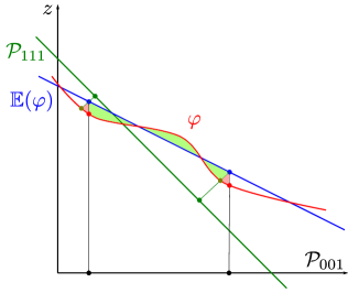
Figure 17. A schematic 2d representation of the proof of Claim 7.4. The set $U$ corresponds to the interval between the black dots on ${\mathcal{P}}_{001}$, $V=\overline{{\mathcal{L}}}(U)$ is the interval between the green dots with the construction of the map $\bar{\mathfrak{L}}$ shown using the thin lines and the blue dots. In this example, the sum over $u\in U$ counts the green area together with the right red component while the sum over $v\in V$ counts the green and left red component.

Consider now $U$ fixed and let $V=\bar{\mathfrak{L}}(U)$, with an arbitrary convention on the boundary which will not have any impact.

Claim 7.4.

There exists $C$ (depending on $\mathfrak{a},\mathfrak{b},\mathfrak{c}$) such that, if there exists $V^{\prime}\supset V$ and $M$ such that $\sup_{v^{\prime}\in V^{\prime}}|\varphi_{111}(v^{\prime})-\mathbb{E}[\varphi_{111}(v^{\prime})]|\leq M$ and $\inf_{v\in\partial V,v^{\prime}\in\partial V^{\prime}}|v-v^{\prime}|\geq CM$, then

$$|\sum_{u\in U}(\varphi_{001}(u)-\mathbb{E}[\varphi(u)])-\sum_{v\in V}(\varphi_{111}(v)-\mathbb{E}[\varphi(v)])|\leq|\partial V|CM^{3}\,.$$

Proof.

Fix a point $p_{1}\in\varphi$ such that $v:=\Upsilon_{111}(p_{1})\in V$ but $\Upsilon_{001}(p_{1})\notin U$. Let $p_{2}$ be the unique point in ${\mathcal{P}}_{\mathfrak{a}\mathfrak{b}\mathfrak{c}}$ such that $\Upsilon_{111}(p_{2})=v$, by assumption $\|p_{1}-p_{2}\|_{1}\leq 3M$ and consequently $\|\Upsilon_{001}(p_{1})-\Upsilon_{001}(p_{2})\|\leq 2M$. On the other hand, by definition $\Upsilon_{001}(p_{2})=\bar{\mathfrak{L}}^{-1}(v)$ so it must be in $U$. Overall we see that $v$ must be at distance at most $2M$ of $\partial V$.

Conversely, take $p_{1}\in\varphi$ such that $u:=\Upsilon_{001}(p_{1})\in U$ and $\Upsilon_{111}(p_{1})\notin V$ and suppose by contradiction that $|\phi_{001}(u)-\mathbb{E}[\phi_{001}(u)]|\geq CM$ for a constant $C$ to be chosen large enough later. As before let $p_{2}$ be the point of ${\mathcal{P}}_{\mathfrak{a}\mathfrak{b}\mathfrak{c}}$ such that $\Upsilon_{001}(p_{2})=u$ and let $v_{2}=\Upsilon_{111}(p_{2})=\bar{\mathfrak{L}}(u)$. Let $p_{2}^{\prime}$ be the point of $\varphi$ such that $\Upsilon_{111}(p_{2}^{\prime})=v_{2}$, by assumption, since $v_{2}\in V$, we must have $\|p_{2}^{\prime}-p_{2}\|_{1}\leq 3M$. Since $\|p_{1}-p_{2}\|\geq CM$ and they only differ in the $z$ coordinate, there must exists a path in $\varphi$ starting at $p_{2}^{\prime}$, (going to $p_{1}$) a doing at most $2M$ steps in the $x$ or $y$ directions while it does at least $CM$ steps in the $z$ direction, either all increasing or all decreasing depending on the sign of $\varphi_{001}(u)-\mathbb{E}[\varphi_{001}(u)]$. If $C$ is large enough, this is a contradiction with the fact that $\varphi$ stays close to ${\mathcal{P}}_{\mathfrak{a}\mathfrak{b}\mathfrak{c}}$ in a large neighborhood of $V$. We can then argue as in the previous paragraph that $v_{2}$ must be within distance $CM$ of $\partial V$.

Overall, we see that the contributions to $|\sum_{u\in U}\big{[}\varphi_{001}(u)-\mathbb{E}[\varphi(u)]\big{]}-\sum_{v\in V}\big{[}\varphi_{111}(v)-\mathbb{E}[\varphi(v)]\big{]}|$ can only come from cubes within distance $CM$ of the boundary of $V$ which concludes the proof of the claim. ∎

Recall from Section 2.1 that we interpret $\varphi_{001}(n\cdot)-\mathbb{E}[\varphi_{001}(n\cdot)]$ as a piecewise constant function defined from $\mathbb{R}^{2}$ to $\mathbb{R}$ and that we write integrals as the $L^{2}$ scalar product. Recall also that, since the full plane Gaussian free field is only defined as a distribution up to a global shift, we only need to prove convergence of

$$\langle\varphi_{001}(n\cdot)-\mathbb{E}[\varphi_{001}(n\cdot)],f\rangle$$

for test functions $f$ with $0$ mean. Clearly, we can further restrict the set of test functions to finite linear combination of the indicator of smooth open sets so for clarity let us focus on the convergence of

$$\langle\varphi_{001}(n\cdot)-\mathbb{E}[\varphi_{001}(n\cdot)],\mathbbm{1}_{U^{+}}-\mathbbm{1}_{U^{-}}\rangle$$

for two disjoint bounded open sets $U^{\pm}$ with smooth boundaries and the same areas. Theorem 1 from [34] tells us that all cumulants of $\varphi_{111}(v)-\varphi_{111}(o)$ of order more that $2$ are bounded uniformly in $v$ and that $\operatorname{Var}(\varphi_{111}(v)-\varphi_{111}(o))$ grows logarithmically in $|v-o|$. In particular, applying Markov to a high enough moment and Borel–Cantelli, we see that almost surely, for all $n$ large enough

$$\sup_{v\in B(o,n)}|\varphi_{111}(v)-\mathbb{E}[\varphi(v)]|\leq n^{1/4}\,.$$

We can then apply Claim 7.4 to both $\sum_{u\in nU^{+}}$ and $\sum_{u\in nU^{-}}$. The error term coming from the claim is $O(n^{{7/4}})$ since $|\partial nU^{\pm}|=O(n)$ and the other errors coming from approximating the sets $U^{\pm}$ by a union of squares contribute $O(n^{5/4})$ so overall

$$\sum_{u}\big{(}\varphi_{001}(u)-\mathbb{E}[\varphi_{001}(u)]\big{)}\big{(}\mathbbm{1}_{nU^{+}}(u)-\mathbbm{1}_{nU^{-}}(u)\big{)} =\sum_{v}\big{(}\varphi_{111}(v)-\mathbb{E}[\varphi_{111}(v)]\big{)}\big{(}\mathbbm{1}_{nV^{+}}(v)-\mathbbm{1}_{nV^{-}}(v)\big{)}$$

$$+O(n^{7/4})\,.$$

Moving from discrete sum to $L^{2}$ inner product, the area of the faces of the dual lattice to $\mathbb{T}$ appears in the right hand side and

$$\langle\varphi_{001}(n\cdot)-\mathbb{E}[\varphi_{001}(n\cdot)],\mathbbm{1}_{U^{+}}-\mathbbm{1}_{U^{-}}\rangle=\frac{\sqrt{3}}{3}\langle\varphi_{111}(n\cdot)-\mathbb{E}[\varphi_{111}(n\cdot)],\mathbbm{1}_{\bar{\mathfrak{L}}U^{+}}-\mathbbm{1}_{\bar{\mathfrak{L}}U^{-}}\rangle+O(n^{-1/4})$$

and hence, since $\varphi_{111}-\mathbb{E}[\varphi_{111}]$ converges to $\sigma\textsc{GFF}\circ\mathfrak{L}$,

$$\langle\varphi_{001}(n\cdot)-\mathbb{E}[\varphi_{001}(n\cdot)],\mathbbm{1}_{U^{+}}-\mathbbm{1}_{U^{-}}\rangle \longrightarrow\frac{\sqrt{3}}{3}\langle\textsc{GFF}\circ\mathfrak{L},\mathbbm{1}_{\bar{\mathfrak{L}}U^{+}}-\mathbbm{1}_{\bar{\mathfrak{L}}U^{-}}\rangle$$

$$=\frac{\sqrt{3}}{3}|\det(\bar{\mathfrak{L}})|\langle\textsc{GFF}\circ\mathfrak{L}\circ\bar{\mathfrak{L}},\mathbbm{1}_{U^{+}}-\mathbbm{1}_{U^{-}}\rangle|\,.\qed$$

The final step, as mentioned above, is to prove that $h-\varphi$ does not contribute to the scaling limit of $h$. Note that for $h$, only the SOS convention makes sense so we stick to this convention and drop the indices.

Lemma 7.5.

Uniformly over $\varphi$ and $u$, $h(u)-\mathbb{E}[h(u)\mid\varphi]$ has an exponential tail, $h(\cdot)-\mathbb{E}[h(\cdot)\mid\varphi]$ has exponentially decaying covariance and for all $U$,

$$\langle h(n\cdot)-\mathbb{E}[h(n\cdot\mid\varphi],\mathbbm{1}_{U}\rangle\xrightarrow[]{\;L^{2}\;}0\,.$$

Proof.

This is essentially a corollary of the analysis of $\pi_{\varphi,\hat{\beta}}$ in Section 6. Indeed, as already mentioned in Remark 2.8, the conditional law of $h$ given $\varphi$ is $\pi_{\varphi,\beta}$. The exponential tail of $h(o)-\mathbb{E}[h(o)\mid\varphi]$ is an immediate consequence of the exponential bound on the size of bubbles given in Eq. 6.20 (note that it is given there for $\pi_{r}$ but since the bound is uniform over $r$ it applies for measure on the torus too). In particular, $h(\cdot)-\mathbb{E}[h(\cdot)\mid\varphi]$ is square integrable and its variance is uniformly bounded in $\varphi$.

For the covariance, fix $x$ and $y$ and let $r=|x-y|$. First note that, again since the size of bubbles has an exponential tail, it is enough to look only on the even where the bubbles at both $x$ and $y$ are smaller than $r/10$. We can then replace the actual law of $h$ given $\varphi$ by the law in $B(o,2r)$ with boundary condition $\varphi$ again with an exponentially small error in $r$. Then, running the dynamic of Section 6 for a time $cr$ with $c$ small enough, except on an event of exponentially small probability, information does not have time to propagate between $B(x,r/2)$ and $B(y,r/2)$ and so on that event $h\mathord{\upharpoonright}_{B(x,r/2)}$ and $h\mathord{\upharpoonright}_{B(y,r/2)}$ are independent. Overall, we see that the covariance decays exponentially with $r$ as desired.

Once we control the pointwise variance and covariances, we deduce immediately that, uniformly over $\varphi$, $\operatorname{Var}(\langle h(n\cdot)-\mathbb{E}[h(n\cdot\mid\varphi],\mathbbm{1}_{U}\rangle)=O(L^{-2})$ which concludes. ∎

Lemma 7.6.

For the law on full plane tilings $\varphi$ given by Theorem 3, $\mathbb{E}[h(o)\mid\varphi]-\varphi(o)$ is bounded and has mean $0$, $\mathbb{E}[h(\cdot)\mid\varphi]-\varphi(\cdot)$ has exponentially decaying covariance and for all $U$,

$$\langle\mathbb{E}[h(n\cdot)\mid\varphi]-\varphi(n\cdot),\mathbbm{1}_{U}\rangle\xrightarrow[]{\;L^{2}\;}0\,.$$

Proof.

$\mathbb{E}[h(o)\mid\varphi]-\varphi(o)$ is bounded again because of the arguments in Section 6. More precisely, since we proved that the size of bubbles has an exponential tail uniformly over $\varphi$, the expected size is bounded as a function of $\varphi$.

To see that $\mathbb{E}[h(o)\mid\varphi]-\varphi(o)$ has mean $0$, first note that by translation invariance $\mathbb{E}[h(u)]-\mathbb{E}[\varphi(u)]$ cannot depend on $u$. Also, we remark that the joint law of $h$ and $\varphi$ is defined only using $h$ and $\varphi$ as union of plaquettes of $\mathbb{Z}^{3}$. In particular, it is invariant under changing the sign of all three axis in space, which transforms $(h(\cdot),\varphi(\cdot))$ to $(-h(-\cdot),-\varphi(-\cdot))$ so $\mathbb{E}[h(\cdot)]-\mathbb{E}[\varphi(\cdot)]$ must be odd (this transformation can also be seen as exchanging the $+$ and $-$ spins in an Ising configuration with interface $h$, or a reflection on the $111$ plane). Overall, the only solution is that $\mathbb{E}[h]=\mathbb{E}[\varphi]$.

For the covariance, we first note that

$$\mathbb{E}[h(o)\mid\varphi]=\varphi(o)+\sum_{r}\sum_{\mathsf{B}:\Upsilon(\mathsf{B})\subset o}(h_{\mathsf{B}}(o)-\varphi(o))(\pi_{2r}(\mathsf{B}\in h)-\pi_{r}(\mathsf{B}\in h))\,,$$

where $h_{\mathsf{B}}(o)$ is the height of $o$ in any configuration containing $\mathsf{B}$ as a bubble. This is almost the same as the decomposition in Section 6 except that there is no integral over $\hat{\beta}$ and we have a slightly different weight per bubble. The arguments of Section 6 apply directly and prove that

$$\Big{|}\sum_{\mathsf{B}:\Upsilon(\mathsf{B})\subset o}(h_{\mathsf{B}}(o)-\varphi(o))(\pi_{2r}(\mathsf{B}\in h)-\pi_{r}(\mathsf{B}\in h))\Big{|}\leq e^{-cr}$$

for some constant $c$, i.e., $\mathbb{E}[h(o)\mid\varphi]-\varphi$ is almost a local function in the same sense as $\mathfrak{g}$. Combined with the polynomial decay of the cumulants of the edge occupation variables in Eq. 8.21, we see that the covariance between $\mathbb{E}[h(o)\mid\varphi]$ and $\mathbb{E}[h(u)\mid\varphi]$ must decay to $0$ as $\|u\|\to\infty$ (at a rate at least $e^{-\varepsilon\sqrt{\log\|u\|}}$). It then immediately follows that $\operatorname{Var}(\langle h(n\cdot)-\mathbb{E}[h(n\cdot\mid\varphi],\mathbbm{1}_{U}\rangle)\to 0$ which concludes the proof. ∎

Concluding the proof of Theorem 1 is then simply a matter of combining the previous results.

Proof of Theorem 1.

We write

$$h-\mathbb{E}[h]=\big{(}\varphi-\mathbb{E}[\varphi]\big{)}+\big{(}h-\mathbb{E}[h\mid\varphi]\big{)}+\big{(}\mathbb{E}[h\mid\varphi]-\varphi\big{)}$$

using the fact that $\mathbb{E}[h]=\mathbb{E}[\varphi]$ mentioned in the proof of Lemma 7.6. The first parenthesis in the right hand side converges to the Gaussian free field by Lemma 7.3 while the other two converge to 0 by Lemmas 7.5 and 7.6. ∎

Let us note that in a sense Theorem 1 gives a much more precise statement about the limit than a simple control of the variance but the fact that the GFF is a distribution means it does not formally imply anything for pointwise moments. For the sake of completeness, we still derive the variance of height increments in the SOS convention.

Proposition 7.7.

As $\|u\|\to\infty$,

$$\operatorname{Var}(h(u)-h(o))=\frac{\sigma^{2}}{p_{\mathfrak{a}}^{2}}\log\|u\|+o(\log\|u\|)\,,$$

where $\sigma$ is given by Theorem 3.

Proof.

First we note that, by Lemmas 7.5 and 7.6, it is enough to prove the result for $\varphi_{001}(u)-\varphi_{001}(o)$ instead. Fix $u$ which according to the convention in Section 2.1 and Fig. 10 we label using half integers. Let us denote by $e_{\uparrow}$ the projection on ${\mathcal{P}}_{111}$ of the unit vector $e_{3}$ The first step is to give concretely how to read the $\varphi_{001}$ height in terms of the $\varphi_{111}$ one.

By definition $\varphi_{001}(u)=z$ if and only if the plaquette $(u_{1}\pm\tfrac{1}{2},u_{2}\pm\tfrac{1}{2},z)$ is in $\phi$ which is then equivalent to then fact that

$$\varphi_{111}\big{(}\Upsilon_{111}(u_{1}+\tfrac{1}{2},u_{2}+\tfrac{1}{2},z)\big{)}=\varphi_{111}\big{(}\Upsilon_{111}(u_{1}-\tfrac{1}{2},u_{2}-\tfrac{1}{2},z)\big{)}=z\,.$$

Also, since both $\mathbb{E}[\varphi_{111}(\cdot)]$ and $\mathbb{E}[\varphi_{001}(\cdot)]$ describe the same plane ${\mathcal{P}}_{\mathfrak{a}\mathfrak{b}\mathfrak{c}}$ and by definition of $\overline{{\mathcal{L}}}$ we have $\mathbb{E}[\varphi_{001}(u)]=\mathbb{E}(\varphi_{111}(\overline{{\mathcal{L}}}(u))$. Using the linearity of the projection we therefore obtain that

$$\Upsilon_{111}(u_{1}+\tfrac{1}{2},u_{2}+\tfrac{1}{2},z)=\overline{{\mathcal{L}}}(u)+\Upsilon_{111}\big{(}\tfrac{1}{2},\tfrac{1}{2},z-\mathbb{E}[\varphi_{001}(u)]\big{)}=\overline{{\mathcal{L}}}(u)+(z-\mathbb{E}[\varphi_{001}(u)]-\tfrac{1}{2})e_{\uparrow}\,.$$

It follows that we would have

$$\varphi_{001}(u)=k+\mathbb{E}[\varphi_{001}(u)]$$ (7.1)

if and only if

$$\varphi_{111}(\overline{{\mathcal{L}}}(u)+(k+\tfrac{1}{2})e_{\uparrow})=\varphi_{111}(\overline{{\mathcal{L}}}(u)+(k-\tfrac{1}{2})e_{\uparrow})=k+\mathbb{E}[\varphi_{111}(\overline{{\mathcal{L}}}(u))]\,.$$

Since $k\to\varphi(u+ke_{\uparrow})-k$ is non-increasing in $k$ we can equivalently reformulate the above as saying that Eq. 7.1 occurs if and only if

$$\varphi_{111}(\overline{{\mathcal{L}}}(u)+(k+\tfrac{1}{2})e_{\uparrow})-(k+\tfrac{1}{2})<\mathbb{E}[\varphi_{111}(\overline{{\mathcal{L}}}(u))]\text{ and }\varphi_{111}(\overline{{\mathcal{L}}}(u)+(k-\tfrac{1}{2})e_{\uparrow})-(k-\tfrac{1}{2})>\mathbb{E}[\varphi_{111}(\overline{{\mathcal{L}}}(u))]\,.$$

Note that for any $v\in{\mathcal{P}}_{111}$, $\mathbb{E}[\varphi_{111}(v+e_{\uparrow})-\varphi_{111}(v)]=1-p_{\mathfrak{a}}$ . Fix $v_{0}=\overline{{\mathcal{L}}}(u)+\tfrac{1}{2}e_{\uparrow}$. First let us consider the good event $G$ where both $|\varphi_{111}(v_{0})-\mathbb{E}[\varphi_{111}(v_{0})]|\leq\log\|v_{0}\|$ and

$$\sup_{v\in B(v_{0},\log^{2}\|v_{0}\|)}|\varphi_{111}(v)-\mathbb{E}[\varphi_{111}(v)]-\varphi_{111}(v_{0})+\mathbb{E}[\varphi_{111}(v_{0})]|\leq\log^{1/4}(\|v_{0}\|)\,.$$

The probability of $G$ goes to $1$ as $\|u\|\to\infty$ because the variance of $\varphi_{111}(v_{0})$ is of order $\log\|v_{0}\|$ and all cumulants of $\varphi_{111}(v)-\varphi_{111}(v_{0})$ of order larger than $2$ are bounded (in fact the 10th moment is enough for the above bound). Let $v_{\pm}$ be the points

$$v_{0}+\frac{\varphi_{111}(v_{0})-\mathbb{E}[\varphi_{111}(p_{0})]}{p_{\mathfrak{a}}}e_{\uparrow}\pm\frac{2\log^{1/4}(\|v_{0}\|)}{p_{\mathfrak{a}}}e_{\uparrow}\,.$$

On $G$ they are both in $B(v_{0},\log^{2}\|v_{0}\|)$ and therefore

$$\varphi_{111}(v_{+}) \leq\varphi_{111}(v_{0})+\frac{1}{p_{\mathfrak{a}}}\mathbb{E}[\varphi_{111}(v_{+})-\varphi_{111}(v_{0})]+\log^{1/4}(\|v_{0}\|)$$

$$\leq\varphi_{111}(v_{0})+\frac{1-p_{\mathfrak{a}}}{p_{\mathfrak{a}}}\big{(}\varphi_{111}(v_{0})-\mathbb{E}[\varphi_{111}(v_{0})]\big{)}+\frac{2-2p_{\mathfrak{a}}}{p_{\mathfrak{a}}}\log^{1/4}(\|v_{0}\|)+\log^{1/4}(\|v_{0}\|)$$

$$<\mathbb{E}[\varphi_{111}(v_{0})]+\frac{1}{p_{\mathfrak{a}}}\big{(}\varphi_{111}(v_{0})-\mathbb{E}[\varphi_{111}(v_{0})]\big{)}+\frac{2}{p_{\mathfrak{a}}}\log^{1/4}(\|v_{0}\|)\,,$$

and similarly

$$\varphi_{111}(v_{-})-\Big{(}\frac{\varphi_{111}(v_{0})-\mathbb{E}[\varphi_{111}(p_{0})]}{p_{\mathfrak{a}}}e_{\uparrow}-\frac{\log^{1/4}(\|v_{0}\|)}{p_{\mathfrak{a}}}\Big{)}>\mathbb{E}[\varphi_{111}(v_{0})]\,.$$

Therefore, still on the event $G$,

$$\varphi_{001}(u)-\mathbb{E}[\varphi_{001}(u)]=\frac{\varphi_{111}(v_{0})-\mathbb{E}[\varphi_{111}(v_{0})]}{p_{\mathfrak{a}}}n+O(\log^{1/4}(\|u\|))\,.$$

Overall we see that $\mathbb{E}[(\varphi_{001}(u)-\mathbb{E}[\varphi_{001}(u)])\mathbbm{1}_{G}]=\frac{\sigma^{2}}{p_{\mathfrak{a}}^{2}}\log\|u\|+o(\log\|u\|)$ as desired.

We now turn to the analysis of the bad event $G^{c}$. As for the good event (or Lemma 7.3), we will use some uniform control on $\varphi_{111}-\mathbb{E}[\varphi_{111}]$ to move between the two convention but this is a bit more complicated because the domain has to depend on the deviation at the reference point $v_{0}$. For $k\geq 1,\ell\geq 0$ and $(k,\ell)\neq(1,0)$, let $B_{k,\ell}$ be the event where both $(k-1)\log\|v_{0}\|\leq|\varphi_{111}(v_{0})-\mathbb{E}[(\varphi_{111}(v_{0})]|<k\log\|v_{0}\|$ and

$$\sup_{v\in B(v_{0},k\ell\log^{2}(\|v_{0}\|))}|\varphi_{111}(v)-\mathbb{E}[\varphi_{111}(v)]-\varphi_{111}(v_{0})+\mathbb{E}[\varphi_{111}(v_{0})]|\geq k\ell\log^{1/4}(\|v_{0}\|)\,,$$

but where the analogous statement for $\ell+1$ does not hold. Applying a moment bound with powers $6$ we see that (if $\|v_{0}\|$ is large enough)

$$\mathbb{P}(B_{k,0})\leq\frac{1}{k^{6}\log^{2}(\|v_{0}\|)}\,,$$

while, with an order $16$ moment and a union bound we find that for $\ell\geq 1$

$$\mathbb{P}(B_{k,\ell})\leq\frac{1}{k^{14}\ell^{14}\log^{2}(\|v_{0}\|)}\,.$$

On the event $B_{k,\ell}$, reasoning as in the case of $G$ we have $\varphi_{001}(u)-\mathbb{E}[\varphi_{001}(u)]\leq 2k(\ell+1)\log^{2}(\|v_{0}\|)$ and therefore the total contribution of all the events $B_{k\ell}$ to the variance is bounded. On the other hand, by Borel–Cantelli and the above bound on the probabilities, we see that (up to a negligible event) $G^{c}\subset\bigcup B_{k\ell}$, which concludes the proof. ∎

8. Renormalization group analysis: proof of Theorem 3

In this section, we show how to improve the results of [34, 35] to be able to apply the output of Theorem 2.1. We start with a fairly lengthy setup: Section 8.1 gives a very short introduction to Kasteleyn theory in non-interacting dimers, it can be safely skipped if one already knows this theory. Section 8.2 presents our strategy to deal with the microcanonical setting. Section 8.3 introduces the formalism of Grassmann integrals and list the property needed later, again it can be safely skipped if the reader is already familiar with the formalism. The main arguments start in Section 8.4 where we rewrite our problem using Grassmann integrals, then Section 8.5 gives an overview of the induction. Only then can we provide the core of the section with the improved bounds on the determinants in Section 8.6 and the adaptation to the microcanonical setting in Section 8.7.

When discussing the GMT framework for proving Theorem 1.4 and the obstacles standing in the way of proving the refined Theorem 3, the reader should have the following two examples in mind:

Example 8.1 (Prototypical application of Theorem 1.4).

For admissible $\mathfrak{a},\mathfrak{b},\mathfrak{c}>0$ and a small enough fixed $\delta>0$, the distribution $\mu_{N}$ is on tilings $\varphi$ of the torus $\mathbb{T}_{N}$ given by

$$\mu_{N}(\varphi)\propto\mathfrak{a}^{n_{\mathfrak{a}}(\varphi)}\mathfrak{b}^{n_{\mathfrak{b}}(\varphi)}\mathfrak{c}^{n_{\mathfrak{c}}(\varphi)}\exp\Big{[}\delta\sum_{x}\sum_{y:\,\operatorname{dist}(x,y)=1}\mathbbm{1}_{\{\operatorname{type}(\varphi,x)=\operatorname{type}(\varphi,y)\}}\Big{]}$$

where $n_{\mathfrak{s}}(\cdot)$ is the number of lozenges of type $\mathfrak{s}$, and $\operatorname{type}(\cdot,x)$ is the lozenge type at the face $x$.

Example 8.2 (Prototypical application of Theorem 3).

For admissible $p_{\mathfrak{a}},p_{\mathfrak{b}},p_{\mathfrak{c}}>0$ and a small enough fixed $\delta>0$, the distribution $\mu_{N}$ is on tilings $\varphi$ of the torus $\mathbb{T}_{N}$ whose lozenge types are $n_{\mathfrak{b}}(\varphi)=\lfloor p_{\mathfrak{b}}N^{2}\rfloor$ and $n_{\mathfrak{c}}(\varphi)=\lfloor p_{\mathfrak{c}}N^{2}\rfloor$ (with $n_{\mathfrak{a}}=N^{2}-n_{\mathfrak{b}}-n_{\mathfrak{c}}$) that is given by

$$\mu_{N}(\varphi)\propto\exp\Big{[}\delta\sum_{x}\sum_{y}\mathbbm{1}_{\{\operatorname{type}(\varphi,x)=\operatorname{type}(\varphi,y)\}}\frac{1}{\operatorname{dist}(x,y)^{2}}\Big{]}\,.$$

8.1. Crash course on Kasteleyn theory

In the following, we will sometime need coordinates on the hexagonal lattice. We use the following convention. First the two bipartite class will be called black and white and we will actually use different variables $b$ and $w$ for white and black vertices. We assume without loss of generality that the lattice is composed of regular hexagons with a horizontal side and that the black vertex is on the right of that edge. We fix a horizontal edge and say that both the white and black vertices adjacent to that edge have coordinate $(0,0)$. For other points, we use non-orthogonal coordinates as indicated in Fig. 18. We say that horizontal (resp. NW to SE and NE to SW) edges have types $\mathfrak{a}$, $\mathfrak{b}$ and $\mathfrak{c}$ respectively.

Figure 18. Left: The coordinate system. Right: The types of edges.

Consider a simply connected piece of the hexagonal lattice $D$ and construct a matrix $K$ indexed by black vertices on the rows and white vertices on the the columns with $K(b,w)=\mathbbm{1}_{\{b\sim w\}}$. In the definition with permutation, we see that the only non-zero terms come from permutations which only associate adjacent white and black vertices, i.e., the non-zero permutations are exactly describing lozenge tilings and $\det(K)=\sum_{\varphi}\varepsilon(\varphi)$ where $\varepsilon(\varphi)$ is the signature of the permutation described by $\varphi$. Now is is also true that the set of tilings of a simply connected domain is closed under rotation of hexagons in the tiling, which in terms of permutation are simply multiplication by a cycle of $3$ elements. Since a cycle of length $3$ has signature $+1$, $\varepsilon(\varphi)$ does not actually depend on $\varphi$ and $|\det(K)|=\#\{\text{tilings of $D$}\}$. Applying the above argument to both $D$ and $D\setminus\{b_{0},w_{0}\}$ for some pair of adjacent vertices $(b_{0}w_{0})$, the comatrix formula for the determinant says that

$$|K^{-1}(w_{0},b_{0})|=\frac{\#\{\text{tilings of $D\setminus\{b_{0},w_{0}\}$}\}}{\#\{\text{tilings of $D$}\}}=\mathbb{P}((b_{0}w_{0})\text{ occupied})$$

with the $\mathbb{P}$ under a uniformly chosen tiling. In fact the comatrix formula has a generalization to minors which gives for any finite set of edges $(b_{i}w_{i})$

$$\mathbb{P}(\forall i,\,(b_{i}w_{i})\text{ occupied})=|\det(K^{-1}(b_{i},w_{j}))|\,.$$ (8.1)

We thus see that a very natural (and fruitful) approach to the dimer model is to try to identify $K^{-1}$.

From this argument, it is also easy to see that if now we put weights (possibly even complex) $\mathfrak{a}$, $\mathfrak{b}$, $\mathfrak{c}$ depending on the types of edges, the associated determinant becomes a partition function of tilings depending on their weights. However, again since hexagon rotations connect all tilings and preserve the number of tiles of each type, this is a trivial operation at the combinatorial level. We will not really use it here but it can however be a relevant change to do in order to get nice asymptotic formulas for $K^{-1}$.

On the torus, it is not quite true that rotation connect all tilings: they can connect all tilings with a given number of tiles of each type but this is not fixed anymore. In terms of height, a tilings can be seen as describing a discrete vector field which is still closed (i.e., its integral along path is invariant under deformation of the path) but in a non-simply connected domain this is not enough for it a admit a true primitive. If we still want to primitive it, we obtain in general an “additively multivalued function”, which can be seen simply as a function in the full plane whose derivatives are periodic and described by the tiling of the torus. It can be seen that the information about the number of tile of each type can be readily read in terms of the global slope of the primitive or equivalently the height gaps between two copies or the integral of the derivative along two non-contractible cycles. We call that information, the instanton component of the configuration. As a consequence, introducing (positive) weights $\mathfrak{a},\mathfrak{b},\mathfrak{c}$ on the edges depending on their types has an interesting effect on the associated dimer measure: it affects the law of the instanton component while keeping the configuration uniform given it. Algebraically, this manifests as follows. Let $K_{\mathfrak{a},\mathfrak{b},\mathfrak{c}}$ denote the weighted matrix with weights depending on the types of edges for the $N\times N$ torus. Then in all tilings the number of tiles of each type must be a multiple of $N$ and

$$\det(K_{\mathfrak{a},\mathfrak{b},\mathfrak{c}})=\sum_{k,\ell}\pm(k,\ell)\mathfrak{a}^{N^{2}-Nk-N\ell}\mathfrak{b}^{Nk}\mathfrak{c}^{N\ell}Z(k,\ell)\,,$$ (8.2)

where $\pm(k,\ell)$ is a sign which in fact only depends on the parity of $k$ and $\ell$ and $Z(k,\ell)$ is the number of tilings $\varphi$ with lozenge types $n_{\mathfrak{a}}(\varphi)=N^{2}-Nk-N\ell$, $n_{\mathfrak{b}}(\varphi)=Nk$ and $n_{\mathfrak{c}}(\varphi)=N\ell$.

It is actually possible to identify completely the function $\pm(k,\ell)$ (since this depends on further convention on the matrix we will not do it here) and to then obtain the unsigned partition function as a combination of $4$ determinants, i.e.,

$$\sum_{k,\ell}\mathfrak{a}^{N^{2}-Nk-N\ell}\mathfrak{b}^{Nk}\mathfrak{c}^{N\ell}Z(k,\ell)=\frac{1}{2}\Big{(}\sum_{\vartheta_{1},\vartheta_{2}\in\{-1,1\}}\pm(\vartheta_{1},\vartheta_{2})\det(K_{\mathfrak{a},\vartheta_{1}\mathfrak{b},\vartheta_{2}\mathfrak{c}})\Big{)}\,.$$

This is the classical route to study the dimer model on the torus (see for example [45]) and in particular this is used in [34, 35]. The analog of Eq. 8.1 in this context becomes, given a pattern $P$ containing $n_{\mathfrak{a}}(P),n_{\mathfrak{b}}(P),n_{\mathfrak{c}}(P)$ tiles of each type subset $S$ of black and white vertices

$$\sum_{\varphi}\pm(k,\ell)\mathfrak{a}^{N^{2}-Nk-N\ell}\mathfrak{b}^{Nk}\mathfrak{c}^{N\ell}\mathbbm{1}_{\{P\in\varphi\}} =\pm(P)\mathfrak{a}^{n_{\mathfrak{a}}(P)}\mathfrak{b}^{n_{\mathfrak{b}}(P)}\mathfrak{c}^{n_{\mathfrak{c}}(P)}\det(K_{\mathfrak{a},\mathfrak{b},\mathfrak{c}}\mathord{\upharpoonright}_{P^{c}})$$

$$=\pm(P)\det(K_{\mathfrak{a},\mathfrak{b},\mathfrak{c}})\prod_{e\in P}K_{\mathfrak{a},\mathfrak{b},\mathfrak{c}}(e)\det(K^{-1}_{\mathfrak{a},\mathfrak{b},\mathfrak{c}}\mathord{\upharpoonright}_{P})\,,$$ (8.3)

where the second line only holds if $K_{\mathfrak{a},\mathfrak{b},\mathfrak{c}}$ is invertible. Let us emphasize that the above formula holds even if the pattern $P$ wraps around the torus and indeed even if it determines completely $k$ and $\ell$. Indeed the signs $\pm(k,\ell)$ in Eq. 8.2 is determined by looking at the sign of the permutation associated to a non-contractible loop as a function of its homotopy class. This is not affected when removing the vertices of $P$ from the graph and therefore the same function $\pm(k,\ell)$ has to appear when expending $\det(K\mathord{\upharpoonright}_{P^{c}})$ and $\det(K)$. Only a global sign can appear to account for the change of convention when removing some rows and columns of the matrix $K$.

By taking the correct $\mathfrak{a},\mathfrak{b},\mathfrak{c}$ it is possible to choose which pairs $(k,\ell)$ will have the main contribution to the partition function or in probabilistic term to choose the typical instanton component and the choice is actually explicit: Fix $p_{\mathfrak{a}},p_{\mathfrak{b}},p_{\mathfrak{c}}$ positive and summing to $1$, let $\Delta$ be a triangle with angles $\pi p_{\mathfrak{a}},\pi p_{\mathfrak{b}},\pi p_{\mathfrak{c}}$ and let $\mathfrak{a},\mathfrak{b},\mathfrak{c}$ be the length of the edges opposite to the associated angle. Then (at least asymptotically) the measure with weights $\mathfrak{a},\mathfrak{b},\mathfrak{c}$ gives probabilities $p_{\mathfrak{a}},p_{\mathfrak{b}},p_{\mathfrak{c}}$ to edges of the corresponding types. It is further known that, for this measure, the instanton component converges to a discrete Gaussian distribution without any normalization but we will not use it here.

Because of the signs, Section 8.1 does not directly gives a formula for the probability of a pattern $P$. However it turns out that the $4$ variants of $K$ are close enough that one can ignore this issue and still write probabilities as determinants of (any version of) $K^{-1}$ with a very small error. This is particularly useful since the $K$ matrices are is diagonal in Fourier space: Indeed, fix $\mathfrak{a},\mathfrak{b},\mathfrak{c}$ (or fix $p_{\mathfrak{a}},p_{\mathfrak{b}},p_{\mathfrak{c}}$ and take $\mathfrak{a},\mathfrak{b},\mathfrak{c}$ according to the above construction), $k=(k_{1},k_{2})$ and let $\hat{w}_{k}=\sum_{w}e^{i\left<k,w\right>}e_{w}$ and $\hat{b}_{k}=\sum_{w}e^{-i\left<k,w\right>}e_{w}$ where $\left<k,w\right>=k_{1}n_{1}+k_{2}n_{2}$ with $(n_{1},n_{2})$ the coordinates of $w$. We have

$$K\hat{w}_{k} =\sum_{w}e^{i\left<k,w\right>}(\mathfrak{a}e_{b}+\mathfrak{b}e_{b+(1,0)}+\mathfrak{c}e_{b+(0,1)})=\sum_{b}e^{-i\left<k,b\right>}(\mathfrak{a}+\mathfrak{b}e^{ik_{1}}+\mathfrak{c}e^{ik_{2}})e_{b}$$

$$=(\mathfrak{a}+\mathfrak{b}e^{-ik_{1}}+\mathfrak{c}e^{-ik_{2}})\hat{b}_{-k}\,,$$

where in the computation, we used $b$ to denote the black vertex with the same coordinates as $w$. We see that it is relevant to introduce the Newton polynomial $P(z_{1},z_{2})=\mathfrak{a}+\mathfrak{b}z_{1}+\mathfrak{c}z_{2}$ and we may note that its zeros are exactly $z_{1}=e^{\pi(p_{\mathfrak{a}}+p_{\mathfrak{b}})}$ and $z_{2}=e^{-i\pi(p_{\mathfrak{a}}+p_{\mathfrak{c}})}$.

8.2. Moving to a microcanonical setting

In the context of this paper, we have to consider the dimer model on a torus with fixed instanton component instead of the more classical “canonical” setting where all possible configurations are possible but have varying weights. In this section we show how to adapt the Kasteleyn theory presented above to this setting. Going back to Eq. 8.2, the idea is that instead of summing $4$ copies to remove the sign, we will introduce complex phases to $\mathfrak{a},\mathfrak{b},\mathfrak{c}$ and then use a Fourier inversion formula to extract $Z(k,\ell)$.

Fix $p_{\mathfrak{a}},p_{\mathfrak{b}},p_{\mathfrak{c}}$ such that $Np_{\mathfrak{a}},Np_{\mathfrak{b}},Np_{\mathfrak{c}}$ are integers and let $\mathfrak{a},\mathfrak{b},\mathfrak{c}$ be the associated weights. For $\vartheta_{1},\vartheta_{2}\in\mathbb{R}$, we write $K(\vartheta_{1},\vartheta_{2})=K_{\mathfrak{a},\mathfrak{b}e^{i\vartheta_{1}},\mathfrak{c}e^{i\vartheta_{2}}}$ and $\mathbf{Z}(k,\ell)=\mathfrak{a}^{-Nk-N\ell}\mathfrak{b}^{Nk}\mathfrak{c}^{N\ell}Z(Np_{\mathfrak{b}}+k,Np_{\mathfrak{c}}+\ell)$. In these new notations, Eq. 8.2 becomes

$$\det K(\vartheta_{1},\vartheta_{2})=\mathfrak{a}^{N^{2}p_{\mathfrak{a}}1}\mathfrak{b}^{N^{2}p_{\mathfrak{b}}(1+i\vartheta_{1})}\mathfrak{c}^{N^{2}p_{\mathfrak{c}}(1+i\vartheta_{2})}\sum_{k,\ell}\pm(k,\ell)\mathbf{Z}(k,\ell)e^{i(Nk\vartheta_{1}+N\ell\vartheta_{2})}\,.$$

It is known from the non-interacting theory (see for example [20]) that $\mathbf{Z}$ is well concentrated at scale $N^{2}$ in the sense that for all $\varepsilon>0$, there exists $\eta>0$ such that if $|k|\geq N\varepsilon$ or $|\ell|\geq N\varepsilon$ then

$$\mathbf{Z}(k,\ell)\leq e^{-\eta N^{2}}\mathbf{Z}(0,0)\,,$$

and therefore

$$\det K(\vartheta_{1},\vartheta_{2})=\mathfrak{a}^{N^{2}p_{\mathfrak{a}}}\mathfrak{b}^{N^{2}p_{\mathfrak{b}}+Ni\vartheta_{1}}\mathfrak{c}^{N^{2}p_{\mathfrak{c}}+Ni\vartheta_{2}}\mathbf{Z}(0,0)\sum_{-\varepsilon N\leq k,\ell\leq\varepsilon N}\pm\frac{\mathbf{Z}(k,\ell)}{\mathbf{Z}(0,0)}e^{i(Nk\vartheta_{1}+N\ell\vartheta_{2})}+O(e^{-\eta N^{2}})\,.$$

Now the Fourier inversion is clear, we choose $\vartheta_{1}$ (resp. $\vartheta_{2}$) such that $e^{Ni\vartheta_{1}}$ (resp. $e^{Ni\vartheta_{2}}$) runs over all $Np_{\mathfrak{b}}$-th (resp., $Np_{\mathfrak{c}}$-th) roots of unity and sum all terms:

$$\sum_{\vartheta_{1},\vartheta_{2}}\det(K(\vartheta_{1},\vartheta_{2})) =\mathfrak{a}^{N^{2}p_{\mathfrak{a}}}\mathfrak{b}^{N^{2}p_{\mathfrak{b}}}\mathfrak{c}^{N^{2}p_{\mathfrak{c}}}\mathbf{Z}(0,0)\sum_{-\varepsilon N<k,\ell<\varepsilon N}\sum_{\vartheta_{1},\vartheta_{2}}\pm\frac{\mathbf{Z}(k,\ell)}{\mathbf{Z}(0,0)}e^{i(Nk\vartheta_{1}+N\ell\vartheta_{2})}+O(e^{-\eta N^{2}})$$

$$=\pm N^{2}p_{\mathfrak{b}}p_{\mathfrak{c}}\mathfrak{a}^{N^{2}p_{\mathfrak{a}}}\mathfrak{b}^{N^{2}p_{\mathfrak{b}}}\mathfrak{c}^{N^{2}p_{\mathfrak{c}}}\mathbf{Z}(0,0)+O(e^{-\eta N^{2}})\,,$$

because only the $k=\ell=0$ term is non-zero in the sum over $\vartheta$ in the right hand side.

With the above formula in mind, we will proceed with the proof by analyzing $\det(K(\vartheta_{1},\vartheta_{2}))$ for fixed $K$ and only treat the sum over them after the whole normalization procedure. This is in fact analogous to [34, 35] where also most of the analysis is focused on a fixed matrix out of the $4$ needed to cancel the signs in Eq. 8.2.

8.3. Grassmann integrals

We begin with a short review of the Grassmann integral notation, see Section 4 of [27] for a more detailed and informed account. It will be used crucially to allow us to write complicated series of minors in a way that looks like perturbed gaussian integrals (similar to say the partition function of the $\phi^{4}$ model) and therefore to import into our problem the intuition and language of Gaussian integration.

Definition 8.3.

Consider two separate sets of $n$ indices $\{b_{i}\}$ and $\{w_{j}\}$. The Grassmann integral is a formal notation using $2n$ variables $\psi_{w_{i}},\psi_{b_{j}}$ defined by the following rule

$$\int\psi_{w_{1}}\ldots\psi_{w_{n}}\psi_{b_{1}}\ldots\psi_{b_{n}}\mathrm{d}\psi=1\,,$$

$$\psi_{w}\psi_{w^{\prime}}=-\psi_{w^{\prime}}\psi_{w}\,,\quad\psi_{b}\psi_{b^{\prime}}=-\psi_{b^{\prime}}\psi_{b}\,,\quad\psi_{w}\psi_{b}=\psi_{b}\psi_{w}\,,$$

and any integral not containing all variables exactly once gives $0$. Analytic functions of the variables $\psi$ are defined by their series expansion, which always gets truncated to a finite number of terms by the anti-symmetry assumption.

The link between determinants and Grassmann integrals is the following.

Proposition 8.4.

Let $K$ be a matrix whose rows are indexed by the $w_{i}$ and columns are indexed by the $b_{j}$, we have

$$\int\exp(\vec{\psi}_{b}\cdot K\cdot\vec{\psi}_{w})\mathrm{d}\psi=\det(K)\,.$$

More generally, for every subsets $I=\{i_{k}\}$ and $J=\{j_{l}\}$ of indices of $w_{i}$’s and $b_{j}$’s, resp., one has

$$\int\prod_{i\in I}\prod_{j\in J}\psi_{w_{i}}\psi_{b_{j}}\exp(\vec{\psi}_{b}\cdot K\cdot\vec{\psi}_{w})\mathrm{d}\psi=\pm\det(K\mathord{\upharpoonright}_{I^{c},J^{c}})\,.$$

Proof.

This is a direct computation: Since only monomials of degree exactly $2n$ have a non-zero integral, the exponential in the first statement is not different from $\frac{1}{n!}(\vec{\psi}_{b}\cdot K\cdot\vec{\psi}_{w})^{n}$. Developing the power, we see that the only non-vanishing terms come from taking every $\psi_{w}$ and $\psi_{b}$ exactly once so we can enumerate all terms using two permutations $\sigma_{w}$ and $\sigma_{b}$. Note that pairs $\psi_{w}\psi_{b}$ commutes with other pairs so we can reorder the $\psi$’s to set $\sigma_{b}$ to the identity, simplifying the $\frac{1}{n!}$ term. This gives

$$\int\exp(\vec{\psi}_{b}\cdot K\cdot\vec{\psi}_{w})=\sum_{\sigma}\sum_{i}K_{i\sigma(i)}\int\psi_{b_{1}}\psi_{w_{\sigma(1)}}\cdots\psi_{b_{n}}\psi_{w_{\sigma(n)}}\mathrm{d}\psi\,.$$

To use the definition of the integral, one must also reorder the $\psi_{b}$ and it can be checked that the resulting change of sign is exactly the signature $\varepsilon(\sigma)$.

The statement about the minor follows the same proof. ∎

Let us note now a few additional algebraic properties that follow from this main definition.

Corollary 8.5.

Suppose $K$ is as above and is also invertible. Then

• $\int\psi_{w}\psi_{b}\exp(\vec{\psi}_{b}\cdot K\cdot\vec{\psi}_{w})\frac{\mathrm{d}\psi}{\det(K)}=K^{-1}_{b,w}$.

• $\int\prod_{i\in I}\prod_{j\in J}\psi_{w_{i}}\psi_{b_{j}}\exp(\vec{\psi}_{b}\cdot K\cdot\vec{\psi}_{w})\frac{\mathrm{d}\psi}{\det(K)}=\det(K^{-1}\mathord{\upharpoonright}_{I,J})=\sum_{\sigma}\varepsilon(\sigma)\prod K^{-1}_{w_{i},b_{\sigma(i)}}$.

• If $K^{-1}=A^{-1}+B^{-1}$, then

  $$\int f(\vec{\psi})e^{\vec{\psi}K\vec{\psi}}\frac{\mathrm{d}\psi}{\det(K)}=\iint f(\vec{\psi}_{1}+\vec{\psi}_{2})e^{\vec{\psi}_{1}A\vec{\psi}_{1}}e^{\vec{\psi}_{2}B\vec{\psi}_{2}}\frac{\mathrm{d}\psi_{1}}{\det A}\frac{\mathrm{d}\psi_{2}}{\det B}\,.$$

The last equality of the second line is called the Wick formula for Gaussian Grassmann integral since it writes a $2|I|$-point correlation in terms of 2 points correlations.

Proof.

The first two lines are classical formula about minors. For the last line, we can check that the Wick expansion matches separately for all monomials. ∎

Because of the expression of the last bullet point, we introduce the notation

$$\int f(\psi)\mathrm{d}P_{g}(\psi):=\int f(\psi)\exp(\psi g^{-1}\psi)\frac{\mathrm{d}\psi}{\det g^{-1}}\,,$$

where $g$ is a matrix. We emphasize that the Wick formula means that we can compute with these notations without going back to the original Grassmann integrals. In fact we can even define the value of any such integral using only the Wick formula even when $g$ is not invertible. A particularly degenerate case of this will be when some rows and columns of $G$ are identically $0$. Suppose $g=g_{1}+g_{2}$ with $g_{1}(i,j)=0$ whenever $i\notin I$ or $j\notin J$. We can still use the formula

$$\int f(\psi)\mathrm{d}P_{g}(\psi)=\int\Big{[}\int f(\psi+\phi)\mathrm{d}P_{g_{2}}(\phi)\Big{]}\mathrm{d}P_{g_{1}}(\psi)\,,$$

using in both integrals the full set of Grassmann variables. However we see that, if any variable $\psi_{w_{i}}$ with $i\notin I$ comes out of the integral over the $\phi$ variables, then the corresponding term will give a $0$ contribution after the second integral. In other words, when expanding (the $w$ part of) the monomials in $\psi+\phi$ in $f$, the only meaningful terms come from the cases where we never choose any $\psi_{w_{i}}$ for $i\notin I$. Therefore, we would have the same combinatorics by replacing $\phi+\psi$ by $\phi+\psi\mathord{\upharpoonright}_{I}$. After that transformation, it makes sense to only consider the outer integral with respect to $g_{1}$ as an integral over variables indexed in $I$ instead of the full set. The inner integral can still be over the full set of variables (it $g_{2}$ does not itself have rows or columns of $0$) with the sum performed only over the common coordinates.

Later we will use linear change of variables extensively. In this context the multilinearity of the Wick formula provides a very nice description.

Lemma 8.6.

Let $X_{1},\ldots,X_{n}$ (resp. $Y_{1},\ldots,Y_{n}$) be linear expressions depending on some Grassmann variables $\psi^{+}_{k}$ (resp. $\psi_{k}^{-}$) and let $g$ be a matrix with rows indexed by the $\psi^{+}$ and columns indexed by the $\psi^{-}$. We have

$$\int\prod_{i=1}^{n}X_{i}\mathrm{d}P_{g}(\psi)=\det\big{(}g(X_{i},Y_{j})\big{)}_{1\leq i,j\leq n}\,,$$

where $g(X_{i},Y_{j}):=\int X_{i}Y_{j}\mathrm{d}P_{g}$ can be computed simply by bilinearity.

The core of the proof of Theorem 3 (and of the original version) is a repeated use of the last point of Corollary 8.5 repeatedly. For this we introduce a further notation to describe the $\log$ of a Grassmann integral.

Definition 8.7.

The truncated expectation (with respect to a propagator $g$) is

$${\mathcal{E}}^{T}_{g}(X_{1},\ldots,X_{k},n_{1},\ldots,n_{k})=\frac{\partial^{\sum n_{i}}}{\partial_{\lambda_{1}}^{n_{1}}\ldots\partial_{\lambda_{k}}^{n^{k}}}\log\int e^{\sum\lambda_{i}X_{i}}\mathrm{d}P_{g}(\psi)|_{\vec{\lambda}=0}\,,$$

where the $X_{i}$ are expressions in terms of the Grassmann variables $X_{i}$. We will drop the subscript when it is clear from context.

It can be checked that the $n_{i}$ introduce exactly the same effect as repeating variables and that ${\mathcal{E}}^{T}(X_{1},\ldots,X_{k},n_{1},\ldots,n_{k})$ has the same algebra as $\prod X_{i}^{n_{i}}$. Also, since by definition the truncated expectation is extracting coefficients from the log of the integral, it satisfies

$$\int e^{X}\mathrm{d}P_{g}(\psi)=\exp\big{(}\sum_{n}\frac{1}{n!}{\mathcal{E}}^{T}(X,n)\big{)}\,,$$

and more generally if we have some extra variables $\phi$ on which we are not integrating,

$$\int e^{X}(\psi+\phi)\mathrm{d}P_{g}(\psi)=\exp\big{(}\sum_{n}\frac{1}{n!}{\mathcal{E}}^{T}(X(\cdot+\phi),n)\big{)}\,.$$

There is an expression of the truncated expectation in terms of the regular expectation (which is basically the formula giving the cumulants of a random variable in terms of its moments) so, as for the regular expectation, if the total number of $+$ and $-$ variables are not equal then ${\mathcal{E}}^{T}(X_{1},\ldots,X_{k})=0$. Also, since $\int 1\mathrm{d}P_{g}(\psi)=1$ by construction, the truncated expectation with no variable is $0$. In particular in the two above formula we can start the sum at $n=1$.

To bound a truncated expectation like the one above, we will to use the following theorem (Battle–Brydges–Federbush formula, see [34, Lemma 3]):

Theorem 8.8.

Consider $I_{1},\ldots I_{s}$ some sets of indices (with as many $+$ term as $-$ term) and write $\psi_{I}=\prod_{i\in I}\psi_{i}$. If $s>1$ then

$${\mathcal{E}}^{T}_{g}(\psi_{I_{1}},\ldots,\psi_{I_{s}})=\sum_{T}\pm(T)\big{(}\prod_{e\in T}g_{e}\big{)}\int\det(G(T,\vec{t}))\mathrm{d}\mathbb{P}_{T}(\vec{t})\,,$$

where

• the index $T$ in the sum is a tree over $\{1,\ldots,s\}$ with each edge marked by two indices in the associated $I_{j}$ and $\pm(T)$ is a sign depending on $T$.

• The product over $e$ runs over the edges of $T$ and $g_{e}$ is the propagator evaluated at the endpoints of $e$.

• $\mathbb{P}_{T}$ is a probability measure on $[0,1]^{s^{2}}$ whose support is on matrices which can be written $t_{j,j^{\prime}}=u_{j}\cdot u_{j^{\prime}}$ for vectors $u_{j}$ of unit $L^{2}$-norms.

• $G(T,\vec{t})$ is a size $\sum|I_{j}|-s+1$ matrix with entries indexed by all pairs of labels not appearing in $T$ and given by $G(T,\vec{t})_{(j,i),(j^{\prime},i^{\prime})}=\vec{t}_{j,j^{\prime}}g((j,i),(j^{\prime},i^{\prime}))$.

Note that we use two indices for each parameter of $g$ just above because we need to identify one of the $I_{j}$ and then the exact $i$ in it.

Let us expand a bit the definition of the matrix $G(T,\vec{t})$. Start from the matrix of size $\sum|I_{j}|$ with rows and columns indexed respectively by the $\psi_{k}^{+}$ and $\psi_{k}^{-}$ in the $I_{j}$. We emphasize that if some $\psi_{k}$ appears in several of the $I_{j}$, we do want to repeat it also in the matrix so that we can really think of it as having blocks indexed in $\{1,\ldots,s\}$. Next, apply a Gram-type construction on the blocks, multiplying every entry in the block $j,j^{\prime}$ by $t_{j,j^{\prime}}=u_{j}\cdot u_{j^{\prime}}$. Note that already at this point, having repeated entries in the $I_{j}$ does not make the determinant vanish. Finally we remove the rows and columns associated with the (labeled) edges of the tree $T$ to get $G(T,\vec{t})$.

In turn, $\det(G(T,\vec{t}))$ will be bounded by the Gram–Hadamard inequality, recalled next.

Theorem 8.9 (Gram–Hadamard).

Let $v_{i}$, $\tilde{v}_{i}$ be two families of vectors in some Euclidean space. Let $G$ be the Gram matrix $G_{i,i^{\prime}}=v_{i}\cdot\tilde{v}_{i^{\prime}}$. Then $|\det(G)|\leq\prod_{i}\lVert v_{i}\rVert\cdot\lVert\tilde{v}_{i}\rVert$.

8.4. Grassmann formulation of the problem

As mentioned at the start of the section our goal is to compute the generating function of the model, from which edge correlations will be obtained as derivatives. In order to simplify the notations and to better highlight our core arguments however, we will only provide a complete derivation for the partition function and only consider the full generating function at the end in Section 8.7. This is a deviation from [35] who directly work with the generating function. We will also take advantage of our more restricted setting to drop some of the notations from [35] but we will provide the matching terms in [35] via footnotes.

The first step is the analog of [35, Prop. 1] and consists in rewriting the partition function in terms of Grassmann integral.

Lemma 8.10.

There exist weights $\mathsf{w}_{\vartheta}$ on patterns such that

$$\mathfrak{a}^{N^{2}p_{\mathfrak{a}}}\mathfrak{b}^{N^{2}p_{\mathfrak{b}}}\mathfrak{c}^{N^{2}p_{\mathfrak{c}}} \sum_{\varphi:k=Np_{\mathfrak{b}},\ell=Np_{\mathfrak{c}}}\exp\Big{[}\sum_{r,x}\mathfrak{g}_{r}(\varphi\mathord{\upharpoonright}_{B(x,r)})\Big{]}$$

$$=\tfrac{1}{N^{2}p_{\mathfrak{b}}p_{\mathfrak{c}}}\sum_{\vartheta}\int\exp\Big{(}\vec{\psi}_{b}\cdot K_{\mathfrak{a},\mathfrak{b},\mathfrak{c}}(\vartheta)\cdot\vec{\psi}_{w}+\sum_{\mathfrak{P}}\mathsf{w}_{\vartheta}(\mathfrak{P})\psi_{S}\Big{)}\mathrm{d}\psi+O(e^{-\eta N^{2}/2})\,,$$

where $\psi_{S}:=\prod_{b\in S}\psi_{b}\prod_{w\in S}\psi_{w}$. The sum over $\vartheta=(\vartheta_{1},\vartheta_{2})$, the matrix $K_{\mathfrak{a},\mathfrak{b},\mathfrak{c}}$ and $\eta$ are given by Section 8.2.

Proof.

In what follows, we use $P$ as the argument to a function $\mathfrak{g}_{r}$ (in our context, the value of $\varphi\mathord{\upharpoonright}_{B(o,r)}$) which we think of as a finite tiling pattern. Given $P$, we can read off $r$ and hence can drop the subscript $r$ from the corresponding $\mathfrak{g}_{r}$. We start with the weighted partition function associated to a fixed $K$ and in this computation we consider $\mathfrak{a},\mathfrak{b},\mathfrak{c}$ as complex to save on notations

$$\sum_{\varphi}\pm(k,\ell) \mathfrak{a}^{N^{2}-Nk-N\ell}\mathfrak{b}^{Nk}\mathfrak{c}^{N\ell}\exp\Big{[}\sum_{r,x}\mathfrak{g}_{r}(\varphi\mathord{\upharpoonright}_{B(x,r)})\Big{]}$$

$$:=\sum_{\varphi}\pm(k,\ell)\mathfrak{a}^{N^{2}-Nk-N\ell}\mathfrak{b}^{Nk}\mathfrak{c}^{N\ell}\exp\Big{[}\sum_{P,x}\mathfrak{g}(P)\mathbbm{1}_{\{\tau_{x}P\in\varphi\}}\Big{]}$$

$$=\sum_{\varphi}\pm(k,\ell)\mathfrak{a}^{N^{2}-Nk-N\ell}\mathfrak{b}^{Nk}\mathfrak{c}^{N\ell}\prod_{P,x}1+(\exp(\mathfrak{g}(P))-1)\mathbbm{1}_{\{\tau_{x}P\in\varphi\}}$$

$$=\mathfrak{c}^{N^{2}p_{\mathfrak{c}}}\sum_{\varphi}\pm(k,\ell)\mathfrak{a}^{N^{2}-Nk-N\ell}\mathfrak{b}^{Nk}\mathfrak{c}^{N\ell}\sum_{\{P_{j},x_{j}\}}\prod_{j}(\exp(\mathfrak{g}(P_{j}))-1)\mathbbm{1}_{\{\forall j\,\tau_{x_{j}}P_{j}\in\varphi\}}$$

$$=\sum_{\{\mathfrak{P}_{j}\}\text{ disjoint}}\prod_{j}\bar{\mathsf{w}}(\mathfrak{P}_{j})\sum_{\varphi}\pm(k,\ell)\mathfrak{a}^{N^{2}-Nk-N\ell}\mathfrak{b}^{Nk}\mathfrak{c}^{N\ell}\mathbbm{1}_{\{\forall j\,\tau_{x_{j}}\mathfrak{P}_{j}\in\varphi\}}$$

$$=\sum_{\{\mathfrak{P}_{j}\}\text{ disjoint}}\prod_{j}\bar{\mathsf{w}}(\mathfrak{P}_{j})\prod_{e\in\bigcup\mathfrak{P}_{i}}K_{\mathfrak{a},\mathfrak{b},\mathfrak{c}}(e)\det(K_{\mathfrak{a},\mathfrak{b},\mathfrak{c}}\mathord{\upharpoonright}_{\bigcap\mathfrak{P}_{i}^{c}})$$

$$=\int\sum_{\{\mathfrak{P}_{i}\}\text{ disjoint}}\prod_{j}\mathsf{w}(\mathfrak{P}_{j})\psi_{\mathfrak{P}_{j}}e^{\vec{\psi}_{b}\cdot K_{\mathfrak{a}\mathfrak{b},\mathfrak{c}}\cdot\vec{\psi}_{w}}\mathrm{d}\psi\,,$$ (8.4)

where $\mathfrak{P}$ are marked patterns $\mathfrak{P}=(\{P_{j}\})$, given some set of $\{P_{j}\}$ the $\mathfrak{P}_{i}$ are the smallest unions of $P_{j}$’s such that the vertex sets of the $\mathfrak{P}_{i}$ are disjoint. We wrote above $\psi_{\mathfrak{P}}=\prod_{w\in\mathfrak{P}}\prod_{b\in\mathfrak{P}}\psi_{w}\psi_{b}$ matching the convention for sets. The weights $\mathsf{w}(\mathfrak{P})$ are defined as

$$\bar{\mathsf{w}}(\mathfrak{P})=\prod_{j}(\exp(\mathfrak{g}(P_{j}))-1)\,,\quad\mathsf{w}(\mathfrak{P})=\prod_{e\in\mathfrak{P}}K_{\mathfrak{a},\mathfrak{b},\mathfrak{c}}(e)\bar{\mathsf{w}}(\mathfrak{P})\,.$$

If we sum over all versions $K(\vartheta)$, the first line becomes the partition function in the statement of the lemma and we get

$$\mathfrak{a}^{N^{2}p_{\mathfrak{a}}}\mathfrak{b}^{N^{2}p_{\mathfrak{b}}}\mathfrak{c}^{N^{2}p_{\mathfrak{c}}} \sum_{\varphi:k=Np_{\mathfrak{b}},\ell=Np_{\mathfrak{c}}}\exp\Big{[}\sum_{r,x}\mathfrak{g}_{r}(\varphi\mathord{\upharpoonright}_{B(x,r)})\Big{]}$$

$$=\frac{1}{N^{2}p_{\mathfrak{b}}p_{\mathfrak{c}}}\sum_{\vartheta}\int\sum_{\{\mathfrak{P}_{j}\}\text{ disjoint}}\prod_{j}\psi_{\mathfrak{P}_{j}}e^{\vec{\psi}_{b}\cdot K_{\vartheta}\cdot\vec{\psi}_{w}}\mathrm{d}\psi+O(e^{-\eta N^{2}})\,.$$

We now claim that

$$e^{\sum_{\mathfrak{P}}\mathsf{w}(\mathfrak{P})\psi_{\mathfrak{P}}}=\sum_{\{\mathfrak{P}_{j}\}\text{ disjoint}}\prod_{j}\mathsf{w}(\mathfrak{P}_{j})\psi_{\mathfrak{P}_{j}}\,.$$ (8.5)

Indeed, when expanding the exponential series, whenever we select two overlapping patterns, we get some $\psi$ with a power $2$ and a vanishing term. For a disjoint collection of patterns, the factorial term in the exponential compensates exactly the enumeration over all the ways to obtain it. Let us emphasize that this “cluster expansion” identity only involves finitely many non-zero terms since by anti-symmetry we only need to keep track of monomials of degree at most $1$ in each variable. ∎

To simplify the analysis, it is useful to re-index slightly the exponent in Lemma 8.10: since $\psi_{\mathfrak{P}}$ only depends on the support of $\mathfrak{P}$, we can factor the sum over all patterns with a given support. We obtain

$$\sum_{\mathfrak{P}}\mathsf{w}(\mathfrak{P})\psi_{\mathfrak{P}}=\sum_{\mathfrak{D}}\mathsf{w}(\mathfrak{D})\psi_{D}\,,$$

where $\mathfrak{D}$ is a marked set $\mathfrak{D}=(D,\{r_{j}\},\{x_{j}\})$ with the constraint that $D$ must be the support of a pattern $\mathfrak{P}$ obtained from the $P_{j}$ with radius $r_{j}$ and center $x_{j}$. The weights become

$$\mathsf{w}(\mathfrak{D})=\mathfrak{a}^{n_{\mathfrak{a}}(D)}\mathfrak{b}^{n_{\mathfrak{b}}(D)}\mathfrak{c}^{n_{\mathfrak{c}}(D)}\sum_{\varphi}\prod_{j}(e^{\mathfrak{g}_{r_{j}}(\varphi\mathord{\upharpoonright}_{B(x_{j},r_{j})}})-1)\,,$$

where the sum is over all tilings of $D$ and $n_{\mathfrak{s}}(D)$ is the number of tiles of type $\mathfrak{s}\in\{\mathfrak{a},\mathfrak{b},\mathfrak{c}\}$ in any tiling of $D$ (which is constant). Let us emphasize a small difficulty with the notation: recall from Section 2.1 that $\varphi\mathord{\upharpoonright}_{B(x,r)}$ denotes the set of tiles of $\varphi$ which intersect $B(x,r)$ so its support is not fully defined by $x$ and $r$. Hence in a marked set $\mathfrak{D}$, the first coordinate $D$ is not redundant.

Recall that the assumption in Theorem 3 over the interaction functions $\mathfrak{g}_{r}$ is $\sum_{r}\|\mathfrak{g}_{r}\|_{\infty}\leq\delta$ for $\delta$ that can be taken arbitrarily small given all other parameters. (In the next lemma we rescale $\delta$ for the convenience of our notation.)

Lemma 8.11.

With Eq. 1.8 in mind, let $\delta>0$ be such that $\sum_{r}\|\mathfrak{g}_{r}\|_{\infty}\leq\delta^{3}/2$. Then

$$|\mathsf{w}(\mathfrak{D})|\leq{\mathcal{Z}}^{\textsc{t}}(D)\delta^{2n(\mathfrak{D})}\prod_{j}\big{[}(2/\delta^{2})\|\mathfrak{g}_{r_{j}}\|_{\infty}\big{]}\,,$$ (8.6)

where ${\mathcal{Z}}^{\textsc{t}}(D)$ is the partition function of tilings of $D$ with weights $\mathfrak{a},\mathfrak{b},\mathfrak{c}$ and $n(\mathfrak{D})$ is the number of centers in $\mathfrak{D}$. Furthermore, there is an absolute constant $C$ so that for any set of $x_{j}$ and $r_{j}$, the number of compatible sets $D$ is at most $C^{|\partial(\bigcup_{j}B(x_{j},r_{j}))|}$ and for all such $D$,

$$C^{-1}\leq\frac{|\partial D|}{|\partial(\bigcup_{j}B(x_{j},r_{j}))|}\leq C\,.$$

Proof.

The first part is a direct application of the uniform bound on the $\mathfrak{g}_{r_{j}}$ from Eq. 1.8 and the enumeration of tilings. Indeed, since $\mathfrak{D}$ contains the information over all centers and radii, summing over patterns $\mathfrak{P}$ compatible with a $\mathfrak{D}$ just amounts to summing over all lozenge tilings of $D$. If $\delta$ is small enough, the weights $\bar{\mathsf{w}}(\mathfrak{P})=\prod_{j}(\exp(\mathfrak{g}_{r_{j}}(P_{j})-1))$ are bounded by $\prod_{j}2\|\mathfrak{g}_{r_{j}}\|$, which is at most $\delta^{2n(\mathfrak{D})}\prod\big{[}(2/\delta^{2})\|\mathfrak{g}_{r_{j}}\|_{\infty}\big{]}$, yielding Eq. 8.6. The second part is because given the $x_{j}$ and $r_{j}$, we only have to choose a tiling of the boundary of $\bigcup B(x_{j},r_{j})$ to determine $D$ and the size of the boundary of a union of balls is bounded by their radii. ∎

Note that if $D$ is simply connected, ${\mathcal{Z}}^{\textsc{t}}(D)=|\det K_{\vartheta}\mathord{\upharpoonright}_{D}|$ by the Kasteleyn theory.

8.5. The original renormalization group analysis

We now turn to the the core of the proof in [35], the estimation of the integral in the right hand side of Lemma 8.10 for a fixed $\vartheta$.

We introduce the following notation

$$\hat{\psi}_{k}^{+} =\sum_{b}e^{-i\left<k,b\right>}\psi_{b}\,, \hat{\psi}_{k}^{-} =\sum_{w}e^{i\left<k,w\right>}\psi_{w}\,,$$

with $k\in[-\pi,\pi]\cap(\frac{2\pi}{N}\mathbb{Z}^{2}+(\vartheta_{1},\vartheta_{2})$ from which we clearly have

$$\psi_{b} =\frac{1}{N^{2}}\sum_{k}e^{i\left<k,b\right>}\hat{\psi}_{k}^{+}\,, \psi_{w} =\frac{1}{N^{2}}\sum_{k}e^{-i\left<k,w\right>}\hat{\psi}_{k}^{-}\,.$$

We computed in Section 8.1 that $K$ is diagonal in Fourier, this becomes in this context

$$\vec{\psi}_{b}\cdot K\cdot\vec{\psi}_{w} =\frac{1}{N^{4}}\sum_{b,w,k,k^{\prime}}e^{i\left<k,b\right>}\hat{\psi}_{k}^{+}K(b,w)e^{-i\left<k^{\prime},w\right>}\hat{\psi}_{k^{\prime}}^{-}$$

$$=\frac{1}{N^{4}}\sum_{k,k^{\prime}}\sum_{w}(\mathfrak{a}+\mathfrak{b}e^{ik_{1}}+\mathfrak{c}e^{ik_{2}})e^{i\left<k-k^{\prime},w\right>}\hat{\psi}_{k}^{+}\hat{\psi}_{k^{\prime}}^{-}$$

$$=\frac{1}{N^{2}}\sum_{k}\mu(k)\hat{\psi}_{k}^{+}\hat{\psi}_{k}^{-},$$

and therefore the inverse is

$$g_{K^{-1}}(\hat{\psi}_{k}^{-},\hat{\psi}_{k^{\prime}}^{+}):=N^{2}\frac{1}{\mathfrak{a}+\mathfrak{b}e^{ik_{1}}+\mathfrak{c}e^{ik_{2}}}\delta_{k,k^{\prime}}\,.$$

We emphasize that the value of $\vartheta$ is hidden in the notation $\sum_{k}$ since the set of modes $k$ depends on $\vartheta$.

The renormalization aspect of the proof comes from the fact that we want to write

$$\frac{1}{\det(K)}\int\exp\big{(}S_{\vartheta}(\psi)+\sum_{\mathfrak{D}}\mathsf{w}(\mathfrak{D})\psi_{D}\big{)}\mathrm{d}\psi=\int\mathrm{d}P_{g^{(-n)}}(\psi^{(-n)})\ldots\int \mathrm{d}P_{g^{(0)}}(\psi^{(0)})$$

$$\exp\Big{(}\sum_{\mathfrak{D}}\mathsf{w}(\mathfrak{D})\big{(}\sum\psi^{(-i)}\big{)}_{D}\Big{)}\,,$$

where $\sum g^{(-i)}=K^{-1}$ and each $g^{(-i)}$ corresponds to integrating a certain scale. Note that (at first approximation) we expect the large scale behavior to be captured by the modes closest to the $0$ of $\mathfrak{a}+\mathfrak{b}e^{ik_{1}}+\mathfrak{c}e^{ik_{2}}$ so the decomposition over scales should amount to writing $(\mathfrak{a}+\mathfrak{b}e^{ik_{1}}+\mathfrak{c}e^{ik_{2}})^{-1}$ in terms of smooth functions supported on concentric annuli. In reality things are more complicated because the higher order term have a significant effect, for example the actual large scale behavior is captured slightly away from the zeros of $(\mathfrak{a}+\mathfrak{b}e^{ik_{1}}+\mathfrak{c}e^{ik_{2}})^{-1}$ so the full analysis involves defining the $g^{(-i)}$ by induction and is very involved.

In this paper, we will only improve on the initial step of the induction so the general idea highlighted above is sufficient and in particular we do not need to define the general inductive procedure. On the other hand, we still need to perform a few transformations (corresponding to [35, Sec. 6.1]) that only really make sense with the full construction in mind and that we ask the reader to just accept as is.

Define

$$\mu(k) =\mathfrak{a}+\mathfrak{b}e^{ik_{1}}+\mathfrak{c}e^{ik_{2}}\,,$$

$$\mu_{0}(k) =\mu(k)+\sum_{\omega\in\{+,-\}}\chi_{0}(k-\bar{p}^{\omega})[-\mu(k)+\left<\bar{\alpha}^{\omega}-\partial\mu(\bar{p}^{\omega}),k\right>]\,,$$

where $\chi_{0}$ is a smoothed version of the indicator of a small ellipse. The parameters $\bar{p}^{\omega}$, $\bar{\alpha}^{\omega}$ and the ellipse are just free parameters for the purpose of this paper since they will get fixed later in the induction.

We then slightly tweak the expression from Lemma 8.10. Let $k_{\omega}$ be the points closest to $\bar{p}_{\omega}$ breaking ties arbitrarily, we distinguish the associated variables by writing $\hat{\Psi}_{\omega}^{\pm}=\hat{\psi}_{k_{\omega}}^{\pm}$. We then use (the degenerate case of) the addition principle to get

$$\int\exp\big{(}S_{\vartheta}(\psi)+\sum_{\mathfrak{D}}\mathsf{w}(\mathfrak{D})\psi_{D}\big{)}\mathrm{d}\psi =(\prod_{k}\mu_{0}(k))\int e^{V(\hat{\psi})}e^{-\frac{1}{N^{2}}\sum_{k}\mu_{0}(k)\hat{\psi}_{k}^{-}\hat{\psi}_{k}^{+}}\frac{\mathrm{d}\psi}{\prod\mu_{0}}$$

$$=(\prod_{k\neq k^{\pm}}\mu_{0}(k))\int\mathrm{d}\hat{\Psi}e^{-\frac{1}{N^{2}}\sum_{\omega}\mu_{0}(k_{\omega})\hat{\Psi}_{\omega}^{-}\hat{\Psi}_{\omega}^{+}}\Big{[}\int\mathrm{d}P_{g^{(\leq 0)}}(\psi)e^{V(\hat{\Psi}+\hat{\psi})}\Big{]}$$ (8.7)

where $g^{(\leq 0)}$ is the propagator defined in Fourier space by $g^{(\leq 0)}(\hat{\psi}_{k}^{+},\hat{\psi}_{k^{\prime}}^{-})=\frac{N^{2}}{\mu_{0}(k)}\mathbbm{1}_{\{k=k^{\prime}\}}\mathbbm{1}_{\{k\neq k^{\pm}\}}$. The potential $V$ is defined by the equality in the first line, i.e.,

$$V(\hat{\psi}) :=-\sum_{k}(\mu(k)-\mu_{0}(k))\hat{\psi}_{k}^{-}\hat{\psi}_{k}^{+}+\sum_{\mathfrak{D}}\mathsf{w}(\mathfrak{D})\psi_{D}$$

$$=-\sum_{k}(\mu(k)-\mu_{0}(k))\hat{\psi}_{k}^{-}\hat{\psi}_{k}^{+}+\sum_{\mathfrak{D}}\mathsf{w}(\mathfrak{D})(\prod_{w\in D}\frac{1}{N^{2}}\sum_{k}e^{-i\left<k,w\right>}\hat{\psi}_{k}^{-})(\prod_{b\in D}\frac{1}{N^{2}}\sum_{k}e^{i\left<k,b\right>}\hat{\psi}_{k}^{+}).$$

Since $V$ has an expression involving both the normal space and the Fourier space, it can be hard to see exactly what is is concretely. Let us therefore rewrite it as much as possible in terms of variables in real space.

$$V(\hat{\Psi}+\hat{\psi}) =-\sum_{k\neq k_{\pm}}(\mu(k)-\mu_{0}(k))\hat{\psi}_{k}^{-}\hat{\psi}_{k}^{+}+\sum_{\omega}(\mu(k_{\omega})-\mu_{0}(k_{\omega}))(\hat{\psi}_{k_{\omega}}^{-}+\hat{\Psi}_{\omega}^{-})(\hat{\psi}_{k_{\omega}}^{+}+\hat{\Psi}_{\omega}^{+})$$

$$\quad+\sum_{\mathfrak{D}}\mathsf{w}(\mathfrak{D})\big{(}\prod_{w\in D}\frac{1}{N^{2}}\sum_{k}e^{-i\left<k,w\right>}\hat{\psi}_{k}^{-}+\frac{1}{N^{2}}\sum_{\omega}e^{-i\left<k_{\omega},w\right>}\hat{\Psi}_{\omega}^{-}\big{)}$$

$$\quad\quad\quad\quad\quad\quad\times\big{(}\prod_{b\in D}\frac{1}{N^{2}}\sum_{k}e^{i\left<k,b\right>}\hat{\psi}_{k}^{+}+\frac{1}{N^{2}}\sum_{\omega}e^{i\left<k_{\omega},b\right>}\hat{\Psi}_{\omega}^{+}\big{)}$$

$$=-\sum_{b,w}\big{[}\sum_{k}(\mu(k)-\mu_{0}(k))e^{i\left<k,b-w\right>}\big{]}\psi_{b}\psi_{w}+\sum_{\mathfrak{D}}\mathsf{w}(\mathfrak{D})\psi_{D}$$

$$\quad+\sum_{\omega}(\mu(k_{\omega})-\mu_{0}(k_{\omega}))[\hat{\Psi}_{\omega}^{-}\hat{\psi}_{k_{\omega}}^{+}+\hat{\psi}_{k_{\omega}}^{-}\hat{\Psi}_{\omega}^{+}+\hat{\Psi}_{\omega}^{-}\hat{\Psi}_{\omega}^{+}]$$

$$\quad+\frac{1}{N^{2}}\sum_{\omega}\sum_{(\mathfrak{D},y)}\mathsf{w}(\mathfrak{D})e^{\pm(y)i\left<k_{\omega},y\right>}\hat{\Psi}_{\omega}^{\pm(y)}\psi_{D\setminus\{y\}}$$

$$\quad+\text{similar terms with up to 4 marked points}.$$

The last written term come from choosing the $\hat{\Psi}$ contribution instead of the $\psi$ contribution at the points $y$ in the big product above. For all points where we took the $\psi$ term, we immediately rewrote them using the normal space variable.

We can now describe the first step of the induction procedure. Let $\chi^{(-1)}$ be another regularized version of the indicator of a small ball. The first decomposition is

$$g^{(\leq 0)}(\psi_{b},\psi_{w})=g^{(0)}(\psi_{b},\psi_{w})+\sum_{\omega}e^{-i\left<p_{\omega},b-w\right>}g_{\omega}^{(\leq-1)}(b,w)$$

where

$$g^{(0)}(\psi_{b},\psi_{w}) =\frac{1}{N^{2}}\sum_{k\neq k^{\pm}}e^{-i\left<k,b-w\right>}\frac{1-\xi^{(-1)}(k-p^{+})-\chi^{(-1)}(k-p^{-})}{\mu_{0}(k)}\,,$$ (8.8)

$$g^{(\leq-1)}(\psi_{b},\psi_{w}) =\frac{1}{N^{2}}\sum_{k\neq k^{\pm}}e^{-i\left<k-p^{w},b-w\right>}\frac{\chi^{(-1)}(k-p_{\omega})}{\mu_{0}(k)}\,.$$ (8.9)

As mentioned above, we want to use the addition formula with the above decomposition and rewrite the resulting expression in an exponential form in order to keep iterating. We start with the formal derivation of the expression setting aside convergence issues. The first step is to write $V$ for a sum of $3$ fields

$$V(\Psi+\phi+\psi) =-\sum_{b,w}\big{[}\sum_{k\neq k^{\pm}}(\mu(k)-\mu_{0}(k))e^{i\left<k,b-w\right>}\big{]}(\psi_{b}\psi_{w}+\phi_{b}\psi_{w}+\psi_{b}\phi_{w}+\phi_{b}\phi_{w})$$

$$\quad+\sum_{\mathfrak{D}}\mathsf{w}(\mathfrak{D})(\psi+\phi)_{\mathfrak{D}}$$

$$\quad+\text{similar expression with up to $4$ $\hat{\Psi}$ terms}$$

$$=\sum_{S,I}\mathsf{w}(S\cup I)\phi_{S}\psi_{I}\,,$$

where with a slight abuse of notation we can say that $S$ can be marked with up to $4$ points and that the corresponding terms in $\phi_{S}$ are replaced by $\hat{\Psi}$. We can also declare that the first terms just correspond to the cases where $S\cup I$ has size $2$. Let us emphasize that the case $S=\emptyset$ and $I=\emptyset$ above are certainly valid since everything comes from developing products but that there is no $n=0$ term. By construction of the truncated expectation, we have

$$\int e^{V(\Psi+\phi+\psi)}\mathrm{d}P_{g^{(0)}}(\psi) =\exp\sum_{n}\frac{1}{n!}{\mathcal{E}}^{T}(V(\Psi+\phi+\cdot),\ldots,V(\Psi+\phi+\cdot))$$

$$=\exp\sum_{n}\frac{1}{n!}\big{[}\sum_{(S_{1},I_{1}),\ldots,(S_{n},I_{n})}\prod_{i}\mathsf{w}(S_{i}\cup I_{i}){\mathcal{E}}^{T}(\psi_{I_{1}},\ldots,\psi_{I_{n}})\phi_{S_{i}}\big{]}$$

$$=\exp\sum_{n}\frac{1}{n!}\sum_{S}\big{[}\sum_{S_{i}\text{partition of $S$}}\sum_{I_{i}}\prod\mathsf{w}(S_{i}\cup I_{i}){\mathcal{E}}^{T}(\psi_{I_{1}},\ldots,\psi_{I_{n}})\big{]}\phi_{S}\,.$$

In the second line, we used the linearity of the truncated expectation and factored out the variables we are not integrating while in the third line we use anti-symmetry of $\phi$ to say that the sets $S_{i}$ never contribute if they are not disjoint. This leads to the following formal expression for $W$, again not considering the issue of summability:

$$W^{(-1)}(S)=\sum_{n\geq 1}\frac{1}{n!}\sum_{\text{partitions }S_{i}}\sum_{I_{i}}\prod\mathsf{w}(S_{i}\cup I_{i}){\mathcal{E}}^{T}(\psi_{I_{1}},\ldots,\psi_{I_{n}})\,.$$ (8.10)

Let us note that for a given $S$, when $n$ is large most of the sets $S_{i}$ must be empty so when trying to understand the convergence of the above expression, we can mostly think of the $I_{i}$ as being directly given by patterns. Recall also from Section 8.3 that the truncated expectation ${\mathcal{E}}^{T}(\psi_{I_{1}},\ldots,\psi_{I_{n}})$ is $0$ if the total number of black and white vertices in the $I_{i}$ do not match and that the weights $\mathsf{w}$ are also only non-zero for sets that admit tilings since they come from enumerating patterns. Combining the two, we see that $W^{(-1)}$ is also supported on sets with the same number of black and white vertices, in particular there is no weight for singletons.

Remark 8.12.

Before providing the bounds on $W^{(-1)}$ justifying the above computation, it is useful to discuss briefly why [35] does not apply directly in our context and where our improvements are. In [35], as a consequence of having only finitely many patterns in the interaction, the weights $\mathsf{w}(\mathfrak{D})$ have a very fast decay—exponentially in the area of $S$. Because of this, the authors could afford to be imprecise in the estimation of the truncated expectation term (we still note that their bound is still far from trivial and that the most naive approach will lead to a divergent series). In our context however, the weights $\mathsf{w}(\mathfrak{D})$ do not have a fast decay—on the contrary, they grow to infinity with the size because there are order $C_{*}^{s}$ patterns of size $s$ for some fixed $C_{*}>1$. We will show in what follows that these divergences of the weights $\mathsf{w}(\mathfrak{D})$ disappear after the first integration step because the $\psi_{\mathfrak{D}}$’s have a very small integral. More precisely, we want to use the following two facts: first, $|\int\mathrm{d}P_{g_{K^{-1}}}\psi_{\mathfrak{D}}|=\mathbb{P}(\text{$\mathfrak{P}$ appears in a tiling})\simeq C_{*}^{-|\mathfrak{D}|}$ by well-known facts from Kasteleyn theory; and second, the Gram–Hadamard bound can be made to give a (slow) exponential decay for large determinants thanks to the fact that $g^{(0)}$ is defined by integrating over only part of the Fourier space.

8.6. Bound on truncated expectation

The goal of this section is to prove the following, which is an analog of [35, Eqs. (6.30) and (6.31)] where they state their bound on the the weights after the first integration:

Proposition 8.13.

The weights $W^{(-1)}$ satisfy the following bound for all $S$ and $\delta$ small enough

$$|W^{(-1)}(S)|\leq\delta C^{|S|}e^{-\frac{\varepsilon_{\chi}}{2}\sqrt{A(S)}}\,$$

where $C$ and $\varepsilon_{\chi}$ are constants and $A(S)$ is the minimal number of vertices in a connected set containing $S$. The constant $\varepsilon_{\chi}$ depends on $\chi^{(-1)}$ but $C$ does not.

Remark 8.14.

Comparing the bound in Proposition 8.13 to [35, Eq. (6.30)], our bound is weaker than the $m=0$ version there: we have an exponential increase in the size of $S$ instead of $C^{|S|}\varepsilon^{\max(1,cn)}$ with $\varepsilon$ chosen small enough after $C$. This is not an issue because after one further induction step, we will obtain a true exponential decay in $|S|$ assuming the regularization was chosen appropriately: Indeed, note that the constant $C$ in Proposition 8.13 does not depend on the regularization chosen so, recalling that the induction corresponds to a way to separate Fourier space, by choosing $\chi^{(-1)}$ to cover a large enough portion of the space, our initial step corresponds to a arbitrary finite number of steps in [35]. However, as seen in [35, Eq. (6.56)], the propagator $g^{(m)}$ after $-m$ steps decays exponentially with $-m$ so, in our notation, for the next integration the Gram–Hadamard bound will carry a factor $\varepsilon_{\chi}^{|S|}$ compensating the $C^{|S|}$ from Proposition 8.13. Note that [35, Eq. (6.60)] giving the full induction hypothesis, does include a factor corresponding in our notations to $2^{-m(2-|S|/2)}$ meaning that the above-mentioned application of Gram–Hadamard with a small propagator $g^{(m)}$ is done there. We will therefore not provide extra details on that point.

Proof.

Recall the expression in Eq. 8.10 for the weights after integration,

$$W^{(-1)}(S) =\sum_{n}\frac{1}{n!}\sum_{\text{partitions }S_{i}}\sum_{I_{i}}\prod_{i}\mathsf{w}(S_{i}\cup I_{i}){\mathcal{E}}^{T}(\psi_{I_{1}},\ldots,\psi_{I_{n}})$$

$$\leq\sum_{n}\frac{1}{n!}\sum_{\text{partitions }S_{i}}\sum_{I_{i}}|{\mathcal{E}}^{T}(\psi_{I_{1}},\ldots,\psi_{I_{n}})|\prod_{i}\Big{[}{\mathcal{Z}}^{\textsc{t}}(D)\delta^{2n(I_{i})}\prod_{j}\big{(}2\delta^{-2}\|\mathfrak{g}_{r^{(i)}_{j}}\|_{\infty}\big{)}\Big{]}\,,$$ (8.11)

where the inequality used the bound from Lemma 8.11 on the weights $\mathsf{w}(S_{i}\cup I_{i})$. We wrote $n(I)$ for the number of centers above, with the same convention as $n(\mathfrak{D})$ from Lemma 8.11. In order to show that the series on the right hand of Eq. 8.11 converge, it suffices to prove an exponential decay of ${\mathcal{E}}^{T}(\psi_{I_{1}},\ldots,\psi_{I_{n}})$ with the area of the $I_{i}$, at a rate slightly larger than the entropy of tilings.

The first step is to introduce a change of variables. Assume first for simplicity that none of the sets $S_{i}\cup I_{i}$ contains a non-contractible loop of $\mathbb{T}_{N}$. Note that while the $S_{i}\cup I_{i}$ must be tileable, there is no need for $I_{i}$ to be since the partition only comes from expending a product. Since there are at most $3^{|S_{i}|}$ dimers configurations covering $S$, one of them has to account for a fraction at least $(3\max(\mathfrak{a},\mathfrak{b},\mathfrak{c}))^{-|S_{i}|}$ of ${\mathcal{Z}}^{\textsc{t}}(S_{i}\cup I_{i})$. We let $\tilde{I}_{i}$ be the set of vertices not covered by this particular tiling. Note that $|\tilde{I}_{i}|\geq|I_{i}|-|S_{i}|$, $|\partial\tilde{I}_{i}|\leq|\partial I_{i}|+3|S_{i}|$ and

$$|\det(K\mathord{\upharpoonright}_{\tilde{I}_{i}})|\geq{\mathcal{Z}}^{\textsc{t}}(S_{i}\cup I_{i})(3\max(\mathfrak{a},\mathfrak{b},\mathfrak{c}))^{-|S_{i}|}\,,$$

For a set $S_{i}\cup I_{i}$ which contains a non-contractible loop, we denote by $\operatorname{cut}(S_{i}\cup I_{i})$ the length of a minimal cut removing all noncontractible loops. Enumerating also over the positions of tiles intersecting this cut, we see that we can find $\tilde{I}$ such that

$$|\det(K\mathord{\upharpoonright}_{\tilde{I}})|\geq{\mathcal{Z}}^{\textsc{t}}(S_{i}\cup I_{i})C^{-|S_{i}|+\operatorname{cut}(S_{i}\cup I_{i})}\,,$$ (8.12)

For $b\in\tilde{I}_{i}$, we let

$$\tilde{\psi}_{b}^{(i)}=\sum_{w\in\tilde{I}_{i}}K(b,w)\psi_{w}\,.$$

Note that for $w\in\tilde{I}_{i}$, $\psi_{w}=\sum_{b\in\tilde{I}_{i}}(K\mathord{\upharpoonright}_{\tilde{I}_{i}})^{-1}(w,b)\tilde{\psi}^{(i)}_{b}$ and therefore (up to a global sign depending on the implicit ordering used in notations such as $\prod_{w\in\tilde{I}_{i}}\psi_{w}$)

$$\prod_{w\in\tilde{I}_{i}}\psi_{w} =\prod_{w\in\tilde{I}_{i}}\sum_{b\in\tilde{I}_{i}}(K\mathord{\upharpoonright}_{\tilde{I}_{i}})^{-1}(w,b)\tilde{\psi}^{(i)}_{b}$$

$$=\sum_{\sigma}\prod_{w\in\tilde{I}_{i}}(K\mathord{\upharpoonright}_{\tilde{I}_{i}})^{-1}(w,b)\tilde{\psi}^{(i)}_{\sigma(w)}$$

$$=\det(K\mathord{\upharpoonright}_{\tilde{I}_{i}})^{-1}\prod_{b\in\tilde{I}_{i}}\tilde{\psi}^{(i)}_{b}\,.$$ (8.13)

To go from the first to the second line, we use that $\tilde{\psi}_{b}^{2}=0$ and to go from the second to the third we use the anti-symmetry. Introducing the notation $\tilde{\psi}_{I_{i}}=\prod_{w\in I_{i}\setminus\tilde{I}_{i}}\psi_{w}\prod_{b\in\tilde{I}_{i}}\tilde{\psi}_{b}\prod_{b\in I_{i}}\psi_{b}$, we have

$${\mathcal{E}}^{T}(\psi_{I_{1}},\ldots,\psi_{I_{n}})=\frac{1}{\prod_{i=1}^{n}\det(K\mathord{\upharpoonright}_{\tilde{I}_{i}})}{\mathcal{E}}^{T}(\tilde{\psi}_{I_{1}},\ldots,\tilde{\psi}_{I_{n}})\,.$$ (8.14)

The product of determinants above accounts for the partition function of tilings but we still need to find a $(1-\varepsilon)^{\sum|I_{i}|}$ decay. This will come from a more detailed analysis of the truncated expectation in the right hand side and a Gram–Hadamard bound. For this we need to explicit the action of the propagator in terms of the new variables.

Note that since $K_{\tilde{I}_{i}}$ acts locally, we still have the same stretched exponential decay as for the original, maybe with a factor $3$ in the multiplicative constant. Furthermore, we also have for any $b$ not on the boundary of $\tilde{I}_{i}$,

$$g^{(0)}(\tilde{\psi}^{(i)}_{b},\psi_{b^{\prime}}) =\sum_{w}K(w,b)g^{(0)}(\psi_{w},\psi_{b^{\prime}})$$

$$=\sum_{w}K(w,b)\frac{1}{N^{4}}\sum_{k,k^{\prime}\neq k^{\pm}}g^{(0)}(\psi_{k}^{-},\psi_{k^{\prime}}^{+})e^{-i\left<k,w\right>+i\left<k,b^{\prime}\right>}$$

$$=\frac{1}{N^{2}}\sum_{k\neq k^{\pm}}\frac{1-\chi^{(-1)}(k-p^{+})-\chi^{(-1)}(k-p^{-})}{\mu_{0}(k)}e^{i\left<k,b^{\prime}-b\right>}(\mathfrak{a}+\mathfrak{b}e^{ik_{1}}+\mathfrak{c}e^{ik_{2}})\,.$$

If we choose the regularization function $\chi^{(0)}$ so that its support lies outside of the support of $1-\chi^{(-1)}(k-p^{+})-\chi^{(-1)}(k-p^{-})$, then $\mu_{0}$ in the denominator is exactly the numerator and hence

$$g^{(0)}(\tilde{\psi}^{(i)}_{b},\psi_{b^{\prime}})=\frac{1}{N^{2}}\sum_{k\neq k^{\pm}}(1-\chi^{(-1)}(k-p^{+})-\chi^{(-1)}(k-p^{-}))e^{i\left<k,b^{\prime}-b\right>}\,.$$

Note that we are already in a good setup to apply the Gram–Hadamard inequality since the above is exactly $\tilde{v}^{(i)}_{b}\cdot v_{b^{\prime}}$ for

$$\tilde{v}^{(i)}_{b} =\frac{1}{N}\sum_{k\neq k^{\pm}}\sqrt{1-\chi^{(-1)}(k-p^{+})-\chi^{(-1)}(k-p^{-})}e^{-i\langle k,b\rangle}e_{k}\,,$$ (8.15)

$$v_{b^{\prime}} =\frac{1}{N}\sum_{k\neq k^{\pm}}\sqrt{1-\chi^{(-1)}(k-p^{+})-\chi^{(-1)}(k-p^{-})}e^{i\langle k,b^{\prime}\rangle}e_{k}\,,$$

with $(e_{k})$ forming an abstract standard basis. For $b$ on the boundary of one of the $I$, we can still have a Fourier description of $g$ and therefore a Gram expression

$$g^{(0)}(\tilde{\psi}_{b},\psi_{b^{\prime}}) =\frac{1}{N^{2}}\sum_{k\neq k^{\pm}}(1-\chi^{(-1)}(k-p^{+})-\chi^{(-1)}(k-p^{-}))\frac{Q_{b}(e^{ik_{1}},e^{ik_{2}})}{\mu_{0}(k)}e^{i\left<k,b^{\prime}-b\right>}$$

$$=\tilde{v}_{b}\cdot v_{b^{\prime}}$$

where $Q_{b}$ is a degree $1$ polynomial depending on the set of neighbors of $b$ in $I$ and

$$\tilde{v}_{b}=\frac{1}{N}\sum_{k\neq k^{\pm}}\sqrt{1-\chi^{(-1)}(k-p^{+})-\chi^{(-1)}(k-p^{-})}e^{-i\langle k,b\rangle}\frac{Q_{b}(e^{ik_{1}},e^{ik_{2}})}{\mu_{0}(k)}e_{k}\,.$$

For any $w\in I_{i}\setminus\tilde{I}_{i}$ the same holds with $Q$ being a single monomial. We note that because of the regularization, there exists $C_{\chi}<\infty$ and $\varepsilon_{\chi}>0$ such that for all $b$

$$\lVert v_{b}\rVert_{2} \leq 1-\varepsilon_{\chi}\,, \lVert\tilde{v}_{b}\rVert_{2} \leq\begin{cases}C_{\chi}&\text{if $b\in\partial I$,}\\ 1-\varepsilon_{\chi}&\text{otherwise.}\end{cases}$$ (8.16)

(We retain the subscripts $\varepsilon_{\chi}$ and $C_{\chi}$ to emphasize their dependence.) Using the above expression, let us turn to the bound on ${\mathcal{E}}^{T}(\tilde{\psi}_{I_{1}},\ldots,\tilde{\psi}_{I_{s}})$. As mentioned before, we use Theorem 8.8 and we will bound $\det(G(T,\vec{t}))$ uniformly over $T$ and $\vec{t}$ so we fix them and, following the notations of Theorem 8.8 we let $u_{j}$ be vectors of unit norm such that $t_{j,j^{\prime}}=u_{j}\cdot u_{j^{\prime}}$. Replacing $g^{(0)}$ by the above expressions In the definition of $G=G(T,\vec{t})$, we see that

$$G_{(j,i),(j^{\prime},i^{\prime})}=(u_{j}\cdot u_{j^{\prime}})(\tilde{v}_{(j,i)}\cdot v_{(j^{\prime},i^{\prime})})=(u\otimes\tilde{v})_{(j,i)}\cdot(u\otimes v)_{(j^{\prime},i^{\prime})}.$$

Note that we removed the superscript $(i)$ since is becomes redundant in the block notation of $G$. Since the $u_{j}$ have unit norms, $\lVert(u\otimes\tilde{v})_{j,i}\rVert=\|\tilde{v}_{j,i}\rVert$ so by Gram–Hadamard (Theorem 8.9)

$$|\det(G(T,\vec{t}))|\leq\big{(}1-\varepsilon_{\chi}\big{)}^{\sum|I_{i}|}C_{\chi}^{\sum_{i}|\partial I_{i}|}\,;$$

therefore,

$$|{\mathcal{E}}^{T}(\tilde{\psi}_{I_{1}},\ldots,\tilde{\psi}_{I_{s}})|\leq\Big{(}\sum_{T}\prod_{e\in T}|g^{(0)}(e)|\Big{)}\cdot\big{(}1-\varepsilon_{\chi}\big{)}^{\sum|I_{i}|}C_{\chi}^{\sum_{i}|\partial I_{i}|}\,.$$

Plugging this in Eq. 8.14, and then substituting the bound on ${\mathcal{E}}^{T}$ into Eq. 8.11, we find that

$$|W^{(-1)}(S)|\leq\sum_{n}\frac{1}{n!} \sum_{\text{partitions }S_{i}}\sum_{I_{i}}\Big{(}\sum_{T}\prod_{e\in T}|g^{(0)}(e)|\Big{)}$$

$$\cdot\prod_{i}\delta^{2n(I_{i})}\frac{{\mathcal{Z}}^{\textsc{t}}(S_{i}\cup I_{i})}{\det(K_{\tilde{I}_{i}})}\Big{(}\prod_{j}\big{(}2\delta^{-2}\|\mathfrak{g}_{r^{(i)}_{j}}\|_{\infty}\big{)}\Big{)}\cdot\big{(}1-\varepsilon_{\chi})\big{)}^{|I_{i}|}C_{\chi}^{|\partial I_{i}|}\,,$$ (8.17)

where we emphasize that the labels in the tree $T$ are still referring to the variables $\tilde{\psi}_{b}$ and the superscript in ${\mathcal{Z}}^{\textsc{t}}$ denotes tilings, not the tree $T$.

Establishing Eq. 8.17 was the hard part in the analysis, however we still need to adapt it to a more usable form. First we can replace $\det(K_{\tilde{I}_{i}})$ by its lower bound from Eq. 8.12, and further bound $\delta^{2n(I)}\leq\delta^{1+n(I)}$ to arrive at

$$|W^{(-1)}(S)|\leq\sum_{n\geq 1}\frac{\delta^{n}}{n!}\sum_{\text{partitions }S_{i}}\sum_{I_{i}} \delta^{\sum n(I_{i})}C^{|S_{i}|}\Big{(}\prod_{i,j}\frac{2}{\delta^{2}}\|\mathfrak{g}_{r_{j}}\|_{\infty}\Big{)}$$

$$\cdot\Big{(}\sum_{T}\prod_{e\in T}|g^{(0)}(e)|\Big{)}\cdot\big{(}1-\varepsilon_{\chi}\big{)}^{\sum|I_{i}|}C_{\chi}^{\sum_{i}|\partial I_{i}|+\operatorname{cut}(S_{i}\cup I_{i})}\,.$$ (8.18)

By construction $|g^{(0)}(x,y)|$ decays as the exponential of the square root of $|x-y|$; let us thus fix $\varepsilon_{\chi}$ and $C_{\chi}$ such that $|g^{(0)}(x,y)|\leq C_{\chi}e^{\varepsilon_{\chi}\sqrt{|x-y|}}$ uniformly over $x,y$. For any tree $T$, we have

$$\prod_{e\in T}|g^{(0)}(e)|\leq C_{\chi}^{n}\prod_{i}\Xi_{i}\quad\mbox{where}\quad\Xi_{i}:=e^{-\varepsilon_{\chi}\sqrt{\operatorname{dist}(S_{i}\cup I_{i}\,,\,\bigcup_{j\neq i}(S_{j}\cup I_{j}))}}\,.$$

where the distance between set is as usual the minimal distance between points in these sets. Then

$$\prod_{i:S_{i}\neq\emptyset}\Xi_{i}\leq e^{-\frac{1}{2}\varepsilon_{\chi}\sqrt{A(S)}}(1+\varepsilon_{\chi}/4)^{\sum_{i}|I_{i}|}\,,$$

where $A(S)$ is the size of the minimal connected set containing $S$, whereas

$$\prod_{i:S_{i}=\emptyset}\Xi_{i}\leq(1+\varepsilon_{\chi}/4)^{\sum_{i}|I_{i}|}\mathfrak{C}(\{S_{i}\},\{I_{i}\})\qquad\mbox{for}\qquad\mathfrak{C}(\{S_{i}\},\{I_{i}\}):=\prod_{i:S_{i}=\emptyset}e^{-\frac{1}{2}\varepsilon_{\chi}\sqrt{\operatorname{dist}(S_{i},I_{i})}}\,.$$

Since there are fewer than $n^{n-2}\leq C^{n}n!$ trees $T$ for some absolute constant $C$, we get overall (changing the value of $C_{\chi}$)

$$\sum_{T}\prod_{e\in T}|g^{(0)}(e)|\leq n!C_{\chi}^{n}e^{-\frac{1}{2}\varepsilon_{\chi}\sqrt{A(S)}}(1+\varepsilon_{\chi}/2)^{\sum|S_{i}\cup I_{i}|}\mathfrak{C}(\{S_{i}\},\{I_{i}\})\,.$$

Also, we can bound $\operatorname{cut}(S_{i}\cup I_{i})\leq|S_{i}|+\operatorname{cut}(I_{i})$. Going back to Eq. 8.18 and matching similar terms, we get

$$|W^{(-1)}(S)|\leq C^{|S|}\sum_{n\geq 1} (\delta C\chi)^{n}e^{-\frac{1}{2}\varepsilon_{\chi}\sqrt{A(S)}}\sum_{\text{partitions }S_{i}}\sum_{I_{i}}\mathfrak{C}(\{S_{i}\},\{I_{i}\})$$

$$\cdot\delta^{\sum n(I_{i})}\Big{(}\prod_{i,j}\frac{2}{\delta^{2}}\|\mathfrak{g}_{r_{j}}\|_{\infty}\Big{)}\big{(}1-\varepsilon_{\chi}\big{)}^{\sum|I_{i}|}C_{\chi}^{\sum_{i}|\partial I_{i}|+\operatorname{cut}(I_{i})}\,.$$ (8.19)

Fix $R>0$. For every $I_{i}$, if we denote $I_{i}^{R}=\bigcup_{j:\;r_{j}\geq R}B_{j}$ (where $B_{j}=B(x_{j},r_{j})$ is part of $I_{i}$), and if $\delta$ is small enough (compared to $R$), then

$$\delta^{n(I_{i})}(1-c_{\lambda})^{r(I_{i})}(1-\varepsilon_{\chi}/2)^{|I_{i}|}C_{\chi}^{|\partial I_{i}|+\operatorname{cut}(I_{i})}\leq\delta^{n(I_{i})/2}(1-c_{\lambda})^{r(I_{i})}(1-\varepsilon_{\chi}/2)^{|I_{i}^{R}|}C_{\chi}^{|\partial I_{i}^{R}|+\operatorname{cut}(I^{R}_{i})}\,.$$

Note that we always have $\operatorname{cut}(I^{R}_{i})\leq 2n$. Also if $I_{i}^{R}$ contains a non-contractible loop but has $|\partial I_{i}|\leq n/2$, then all the connected components of its complement must be simply connected. Applying the isoperimetric inequality to each of them, this is only possible if $|I^{R}_{i}|\geq n^{2}/2$. Overall, up to a change of constant we can ignore the term $\operatorname{cut}(I^{R}_{i})$ for $n$ large enough. Now, note the following simple fact:

Fact 8.15.

There exists an absolute constant $C>0$ such that, for every $R>0$ and finite collection $\{B_{j}\}$ of balls of radius at least $R$ in $\mathbb{R}^{2}$, the set $I^{R}=\bigcup_{j}B_{j}$ satisfies $|\partial I^{R}|\leq C|I^{R}|/R$.

Proof.

We will prove the result for balls defined in the continuum and with $|I^{R}|$ and $|\partial I^{R}|$ denoting respectively the Lebesgue measure and the length measure. In the discrete setting of a bounded degree graph, the result is trivial for $R\leq 1$ while for $R\geq 1$ it can be obtained from the continuum analog up to a change of constant. Let $x_{j}$ and $r_{j}$ denote the centers and radii of the balls $B_{j}$, we assume without loss of generality that the $x_{j}$ do not repeat. Let $A_{j}=\{x\in\partial I^{R}\,:\;\operatorname{dist}(x,x_{j})=r_{j}\}$, we have $\bigcup_{j}A_{j}=\partial I^{R}$ and, since the intersection of two circles with different centers contains at most $2$ points, $|A_{j}\cap A_{j^{\prime}}|=0$ for all $j\neq j^{\prime}$. Let $C_{j}$ be the “corner” associated to the arc “$A_{j}$”, i.e., $C_{j}=\bigcup_{x\in A_{j}}[x_{j},x]$ where $[x_{j},x]$ denotes the closed segment between the points $x_{j}$ and $x$. By construction $\bigcup_{j}C_{j}\subset I^{R}$ and $|C_{j}|=2|A_{j}|/R$. Also, since the sum of the length on opposite sides of a quadrilateral is smaller than the sum of the length of the diagonal, for all $j\neq j^{\prime}$ and different $x\in A_{j},x^{\prime}\in A_{j^{\prime}}$, the segments $[x_{j},x]$ and $[x_{j^{\prime}},x^{\prime}]$ are disjoint. In particular $|C_{j}\cap C_{j^{\prime}}|=0$ for all $j,j^{\prime}$. Combining the above, we have

$$|\partial I^{R}|=\sum_{j}|A_{j}|=\sum_{j}2|C_{j}|/R\leq 2|I^{R}|/R$$

as desired. ∎

Choosing $R=R_{\chi}$ large enough, we can therefore bound the perimeter terms by the total area, obtaining that

$$\delta^{n(I_{i})}(1-c_{\lambda})^{r(I_{i})}(1-\varepsilon_{\chi}/2)^{|I_{i}|}C_{\chi}^{|\partial I_{i}|}\leq\delta^{n(I_{i})/2}(1-c_{\lambda})^{r(I_{i})}(1-\varepsilon_{\chi}/4)^{|I_{i}^{R}|}\,.$$

If $\delta$ is small enough, this then gives

$$\delta^{n(I_{i})/4}(1-c_{\lambda})^{r(I_{i})}(1-\varepsilon_{\chi}/4)^{|I_{i}|}2^{|S|}$$

where the $2^{|S|}$ comes from the fact that, in order to apply 8.15, we might have included some points of $S$ in $I^{R}$. Coming back to the full expression in Eq. 8.19, we can now deduce that

$$|W^{(-1)}(S)|\leq(2C)^{|S|}\sum_{n\geq 1}(\delta C_{\chi})^{n} e^{-\frac{1}{2}\varepsilon_{\chi}\sqrt{A(S)}}\sum_{\text{partitions }S_{i}}\sum_{I_{i}}\mathfrak{C}(\{S_{i}\},\{I_{i}\})$$

$$\cdot\delta^{\sum n(I_{i})/4}(1-\varepsilon_{\chi}/4)^{\sum|I_{i}|}\Big{(}\prod_{i,j}\frac{2}{\delta^{2}}\|\mathfrak{g}_{r_{j}}\|_{\infty}\Big{)}\,.$$

We turn to the sum over the $I_{i}$. Recall that each $S_{i}\cup I_{i}$ is a set decorated with pairs of centers and $(x_{j},r_{j})$ together with possibly up to $4$ extra marked points corresponding to a variable $\hat{\Psi}_{\omega}^{\pm}$. Recall further that, given some $\{(x_{j},r_{j})\}$, there are at most $C^{|\partial\bigcup_{j}B(x_{j},r_{j})|}$ compatible $I$ (second part of Lemma 8.11). Finally, while $S_{i}\cup I_{i}$ must be a connected set, it is possible to have $S_{i}=\emptyset$ but in such a case the term $\mathfrak{C}$ provides a penalization by $\exp[-\frac{1}{2}\varepsilon_{\chi}\sqrt{\operatorname{dist}(I_{i},S)}]$.

We first enumerate over the faces of $\frac{1}{\eta}\mathbb{T}$ intersecting $S_{i}\cup I_{i}$ for an $\eta$ to be chosen small enough later and then over all possibles $x_{i}$ in these faces and associated $r_{i}$. By 5.23, if $S_{i}$ is not empty, there are at most $e^{C\eta|S_{i}\cup I_{i}|}$ possible sets of faces for some absolute constant $C$. When $S_{i}$ is empty, because of the penalization by the distance, the same argument applies and we only have to count an extra factor $C_{\chi}$ to choose the position. At each point, choosing whether to introduce a center and summing over all possible $r$ provides a factor of

$$1+\sum_{r\geq 1}\frac{2}{\delta^{2}}\|\mathfrak{g}_{r}\|_{\infty}\leq 1+\delta$$

to the enumeration. (NB. this is the location where the key assumption on the weights $\mathfrak{g}_{r}$ is used.)

Last, choosing $I_{i}$ given $\{(x_{j},r_{j})\}$ provides a factor $C^{|\partial\bigcup_{j}B(x_{j},r_{j})|}$ but these terms can be absorbed into $\delta^{\sum n(I_{i})}(1+\delta)^{\sum|I_{i}|}$ as before. Altogether we obtain

$$\sum_{I_{i}}\mathfrak{C}(\{I_{i}\},\{S_{i}\})\delta^{\sum n(I_{i})} \Big{(}\prod_{i,j}\frac{2}{\delta^{2}}\|\mathfrak{g}_{r_{j}}\|_{\infty}\Big{)}(1-\varepsilon_{\chi}/4)^{\sum|I_{i}|}$$

$$\leq C_{\chi}^{n}\delta\sum_{s}e^{C\eta(|S_{i}|+s)}(1+\delta)^{12s/\eta}(1-\varepsilon_{\chi}/4)^{s}\leq C_{\chi}^{n}2^{|S_{i}|}$$ (8.20)

where the last bound holds if we first choose $\eta$ small enough and then $\beta$ large enough depending on $\varepsilon_{\chi}$. This leads to (still changing the values of the constants):

$$|W^{(-1)}(S)|\leq C^{|S|}e^{-\frac{1}{2}\varepsilon_{\chi}\sqrt{A(S)}}\sum_{n\geq 1}(\delta C_{\chi})^{n}\sum_{\text{partitions }S_{i}}C^{\sum|S_{i}|}\,.$$

Finally, again assuming $\delta$ is small enough and changing the value of the absolute constant $C$,

$$|W^{(-1)}(S)|\leq\delta C^{|S|}e^{-\frac{1}{2}\varepsilon_{\chi}\sqrt{A(S)}}\,,$$

which concludes the proof of Proposition 8.13. ∎

As mentioned in Remark 8.14, the above estimate corresponds to the initialization in the inductive procedure. The rest of the induction then follows exactly as in [35] and provides the following output:

Proposition 8.16.

$$\int\exp\big{(}\vec{\psi}K\vec{\psi}+\sum_{\mathfrak{P}}w(\mathfrak{P})\psi_{S}\big{)}\mathrm{d}\psi=\exp(N^{2}E_{\vartheta}^{(h)})\int\exp\Big{(}\frac{Z^{(h)}}{N^{2}}\sum_{\omega}\mu_{\vartheta,\omega}\hat{\Psi}^{+}_{\omega}\hat{\Psi}^{-}_{\omega}+V_{\vartheta}^{(h)}(\sqrt{Z^{(h)}}\Psi)\Big{)}\mathrm{d}\Psi$$

where $h$ is the index of the last step of the induction, $h=\log_{2}(N)+O(1)$, while $E_{\vartheta}^{(h)}$, $\mu_{\vartheta,\omega}$, $Z^{(h)}$ and $V^{(h)}$ are given by the renormalization procedure. The terms $E_{\vartheta}^{(h)}$, $\mu_{\vartheta,+}$, $\mu_{\vartheta,-}$, $Z^{(h)}$ are real numbers while $V$ is a polynomial in $\Psi$ (which was defined at the start of Section 8.5).

Furthermore, the following holds:

1. The terms $E_{\vartheta}^{(h)}$, $\mu_{\vartheta,+}$, $\mu_{\vartheta,-}$, $Z^{(h)}$ and the coefficients of $V$ are given by absolutely convergent sums over labeled trees. They are analytic functions of the weights of patterns.

2. The set of labeled trees in the first item is independent of $\vartheta$.

Giving full details on the definition of $E,\mu,Z$ and $V$ above would require repeating long and technical parts of [35] so we only give a brief description of $E$. The other terms admit similar expansions. The general form of the formula is in fact not surprising, we performed the integral over all the variables $\psi$ from the left hand side except from the two modes $\Psi$ which remain to be integrated and are present in the right hand side. Furthermore, since we are always rewriting our formula in exponential form, it is natural to end up with the exponential of a polynomial in $\Psi$ so in a sense we just gave names to (parts of) the coefficients of order $0$ and $2$ in that polynomial.

$E_{\vartheta}^{(h)}$ keeps track of the weight of the empty set over the renormalization procedure, looking back at Eq. 8.7, we see that $e^{N^{2}E^{(0)}_{\vartheta}}=\prod_{k\neq k^{\pm}}\mu_{0}(k)$ (again the dependence in $\vartheta$ is hidden in the set of Fourier modes in the product). After the first integration, $E_{\vartheta}^{(-1)}-E_{\vartheta}^{(0)}=W^{(-1)}(\emptyset)$ is the constant in the formula for $W^{(1)}$ which of course just factors out of all further integration. Similarly $E_{\vartheta}^{(h-1)}-E_{\vartheta}^{(h)}$ will be the constant factor appearing in step $h$ of the integration. Similarly to step $1$, it will be a sum over all collections of sets of the step-$h$ weights combined with the scale $h$ propagator. If the step-$h$ weights are themselves rewritten in terms of the weights at a previous scale, we obtain a sum over trees with $h$ generations describing “trajectories” in the space of interaction terms, see [34, Eq. (5.1)] and the discussion preceding it for details.

In fact, the above expansion is a bit too naive, to obtain a convergent expansion, it is necessary to separate at each step the “main” terms (called the local terms in [35]) from the rest. This makes the labeling scheme more complicated (and the proof considerably more challenging) than what would appear by just repeating the expansion used from step $0$ to $1$ repeatedly but at our level of details the naive picture is sufficient.

Remark 8.17.

At this point, we can expand on why the renormalization group approach of [34] manages to give an expression for the free energy as a analytical function of the interaction but a cluster expansion approach would fail.

At first glance, the approaches seem similar: Lemma 8.10, which is an analog of [35, Prop. 1], provides an estimate à la cluster expansion: it replaces $\sum\exp[\sum_{r,x}(\ldots)]$ by $\exp[\sum_{\mathfrak{P}}(\ldots)]$, and begins with rewriting $\exp[\sum\mathfrak{g}(P)]$ as $\prod_{P}(1+(\exp(\mathfrak{g}(P)-1))$ and expanding the product, as done in the classical cluster expansion proofs. However, the fact that the $\psi_{\mathfrak{P}}$ are Grassmann variables instead of usual indicator functions actually simplifies considerably this rewriting: in Eq. 8.5, the left hand side $\exp[\sum_{\mathfrak{P}}\mathsf{w}(\mathfrak{P})\psi_{\mathfrak{P}}]$ directly gives a sum over disjoint patterns (because any term of order more than $2$ cancels: $\psi_{b}^{2}=0$ and $\psi_{w}^{2}=0$), namely $\sum_{\{\mathfrak{P}_{j}\}\text{ disjoint}}\prod_{j}\mathsf{w}(\mathfrak{P}_{j})$. Comparing to the classical cluster expansion formula, this avoids all the “extra” terms involving Ursell functions.

Already getting to this point, where we may use Grassman variables to account for the interaction, is model-specific. Indeed, in our context, one can see these variables as just a nice way to work with the determinants from Kasteleyn theory (see Section 8.1 and Eq. 8.4 for its use in the proof of Lemma 8.10), with the anti-symmetry of the variables designed to match the behavior of the determinant under permutation of the lines and columns (a property of fermionic models).

Even at this point, the term $(1+\delta)^{12s/n}$ from Eq. 8.20, left from enumerating over patterns $\mathfrak{P}$, would destroy the summability condition needed for cluster expansion. This is due to the fact that every pattern $\mathfrak{P}$ has an entropy of $A(\mathfrak{P})$ (its area), yet is only penalized by $\operatorname{diam}(\mathfrak{P})$ (and even that, with a very small constant). In other words, the move to Grassman variables transformed the cluster expansion summability condition into showing that $W^{(-1)}(S)$ from Eq. 8.10 is summable.

The remedy is to use the truncation in Fourier space, and its associated factor of $(1-\varepsilon_{\chi}/4)^{s}$. That is, the term $(1+\delta)^{A(\mathfrak{P})}$ is handled by the finite range effect of $g^{(0)}$, which is $(1-\varepsilon_{\chi})^{A(\mathfrak{P})}$.

Finally, we also needed to handle the enumeration over tilings; to that end we moved in Eqs. 8.12 and 8.13 from $\psi\mathord{\upharpoonright}_{I_{i}}$ to $\tilde{\psi}\mathord{\upharpoonright}_{I_{i}^{\prime}}$ via multiplying by $K$; this change-of-basis was accompanied by a minor of $K$, which exactly counted the number of tilings. Moreover, $g^{(0)}$ is similar to $K^{-1}$, and so in this new basis, it becomes close to the identity.

Note that the truncated expectation ${\mathcal{E}}^{T}(\psi_{I_{1}},\ldots,\psi_{I_{n}})$ was bounded in [34, 35] via Gram–Hadamard by some $C>0$ (which they could afford, as in their setting they have an $e^{-C^{\prime}A(\mathfrak{P})}$ at their disposal) and this bound can easily be seen from the definition of $g$ in Fourier space. We also use the same Gram–Hadamard bound here, but in addition, exploit the fact that it is the $L^{2}$-norm of $\tilde{v}$ from Eq. 8.15 which is bounded in Eq. 8.16 by a more precise $(1-\varepsilon_{\chi})$, using the fact that we found a base where $g^{(0)}$ is close to the identity (whose columns of course have $L^{2}$-norm exactly $1$).

8.7. Back to the microcanonical model

Recall from Lemma 8.10 that the partition function of the interacting model was written as

$$\sum_{\varphi:k=Np_{\mathfrak{b}},\ell=Np_{\mathfrak{c}}}\exp\bigg{(}\sum_{r,x}\mathfrak{g}_{r}(\varphi\mathord{\upharpoonright}_{B(x,r)})\bigg{)}=\frac{1}{N^{2}p_{\mathfrak{b}}p_{\mathfrak{c}}}\sum_{\vartheta}\int\exp\Big{(}S_{\vartheta}(\psi)+\sum_{\mathfrak{P}}\mathsf{w}(\mathfrak{P})\psi_{S}\Big{)}\mathrm{d}\psi+O(e^{-\eta N^{2}/2})\,.$$

Further recall that, by Proposition 8.16, each term $\int\exp\big{(}S_{\vartheta}(\psi)+\sum_{\mathfrak{P}}\mathsf{w}(\mathfrak{P})\psi_{S}\big{)}\mathrm{d}\psi$ on the right is equal to

$$\exp(N^{2}E_{\vartheta}^{(h)})\int d\Psi\exp(\frac{Z^{(h)}}{N^{2}}\sum_{\omega}\mu_{\vartheta,\omega}\hat{\Psi}^{+}_{\omega}\hat{\Psi}^{-}_{\omega}+V_{\vartheta}^{(h)}(\sqrt{Z^{(h)}}\Psi))\,.$$

We are interested in the asymptotic of the free energy $F=\log\big{(}\sum_{\varphi}\exp\sum_{r,x}\mathfrak{g}_{r}(\varphi\mathord{\upharpoonright}_{B(x,r)})\big{)}$ and in correlations such as $\operatorname{Cov}(\mathbbm{1}_{e},\mathbbm{1}_{e^{\prime}})$ were $\mathbbm{1}_{e}$ is the indicator that the edge $e$ is occupied in the tilings (as well as higher order cumulants). We will only provide details on the output of the construction for $F$ and $\operatorname{Cov}(\mathbbm{1}_{e},\mathbbm{1}_{e^{\prime}})$ because higher order cumulants are obtained similarly, see [34] for details.

We start by analyzing the dependence in $\vartheta$ and $N$ of $E_{\vartheta}^{(h)}$ from Proposition 8.16. Recall that $e^{N^{2}E^{(0)}_{\vartheta}}=\prod_{k\neq k^{\pm}}\mu_{0}(k)$ where $\mu_{0}$ is a smooth function of $k$ away from two points $p^{\pm}$ with a singularity of order $1$ at these two points, that $k$ runs over the discrete torus with mesh size $1/N$ shifted by $\vartheta_{1}$ in the first coordinate and $\vartheta_{2}$ in the second coordinate and that $k^{\pm}$ are the two points of that lattice closest to $p^{\pm}$. One can check that $e^{N^{2}E^{(0)}_{\vartheta}}/e^{N^{2}E^{(0)}_{0,0}}$ is bounded and bounded away from $0$ uniformly over $\vartheta$ and $N$.

Recall further that $E^{(h)}_{\vartheta}-E^{(0)}_{\vartheta}$ is an absolutely convergent series where each term is a product of truncated expectations with respect to recursively defined “single scale propagators” $g_{\vartheta}^{(i)}$ (see the explanation around Eqs. 8.8 and 8.9). For $i$ close to $0$, $g^{(i)}_{\vartheta}/g^{(i)}_{(0,0)}=1+O(N^{-2})$ because they are Riemann sums approximations of the integral of a $\mathcal{C}^{2}$ function while for $(i)$ very negative $g^{(i)}_{\vartheta}$ is exponentially decreasing in $(i)$. Overall it can be shown that $E^{(h)}_{\vartheta}-E^{(0)}_{\vartheta}=\Delta+\frac{\log(1+s(\vartheta,N))}{N^{2}}$ where $\Delta$ only depends on the parameters of the model and $s$ is equicontinuous in $N$. Furthermore $s$ can be bounded by an arbitrarily small constant by taking $\beta$ large enough. In fact, the same also holds when subtracting from $\log(1+s)$ a factor $2\log Z_{h}$ to normalize the integral over $\Psi$. Overall this shows that

$$\int\exp\Big{(}\vec{\psi}K\vec{\psi}+\sum_{\mathfrak{P}}\mathsf{w}(\mathfrak{P})\psi_{S}\Big{)} \mathrm{d}\psi=e^{N^{2}E^{(h)}_{(0,0)}}$$

$$\cdot(1+s(\vartheta,N))\frac{1}{Z_{h}^{2}}\int\exp\Big{(}\frac{Z^{(h)}}{N^{2}}\sum_{\omega}\mu_{\vartheta,\omega}\hat{\Psi}^{+}_{\omega}\hat{\Psi}^{-}_{\omega}+V_{\vartheta}^{(h)}(\sqrt{Z_{h}}\Psi)\Big{)}\mathrm{d}\Psi\,.$$

The coefficients of $V^{(h)}$ are by definition associated to the exponentially decreasing factors in the renormalization. Since $h$ is of order $\log_{2}(N)$ it means that they must be polynomially small in $N$. In fact, since the rate of decay are explicit as a function of the size (see the “dimensional estimates” in [35, Eq. (6.60)]) and for $V$ they are at least $N^{-3}$ so these terms must have a vanishing contribution as $N\to\infty$. However the Grassmann integral with only a quadratic term is the exponential is explicit which overall gives

$$\int\exp\Big{(}\vec{\psi}K\vec{\psi}+\sum_{\mathfrak{P}}\mathsf{w}(\mathfrak{P})\psi_{S}\Big{)}\mathrm{d}\psi=e^{N^{2}E^{(h)}_{(0,0)}}(1+s(\vartheta,N))\mu_{\vartheta,+}\mu_{\vartheta,-}(1+O(1/N))\mu_{\vartheta,+}\mu_{\vartheta,-}\,.$$

Furthermore, $\mu_{\vartheta,\pm}$ is given by a convergent series with bounds that are uniform in $\vartheta$ and it is analytic by Proposition 8.16.

Combining all of the above, and plugging it back in our original sum, we find

$$\sum_{\varphi}\exp\sum_{r,x}\mathfrak{g}_{r}(\varphi\mathord{\upharpoonright}_{B(x,r)})=e^{N^{2}E^{(h)}_{(0,0)}}\frac{1}{N^{2}p_{\mathfrak{a}}p_{\mathfrak{b}}}\sum_{\vartheta}\frac{e^{N^{2}E^{(0)}_{\vartheta}}}{e^{N^{2}E^{(0)}_{(0,0)}}}(1+s(\vartheta,N))+O(e^{-\eta N^{2}/2})\,.$$

The term summed in the right hand side is bounded and therefore $\frac{1}{N^{2}}F\to\lim_{h\to\infty}E^{(h)}_{0,0}$.

We now turn to the correlations. Given a function $e\to A_{e}$, define the generating function

$$e^{F(A)}:=\sum_{\varphi}\exp\bigg{(}\sum_{r,x}\mathfrak{g}_{r}(\varphi\mathord{\upharpoonright}_{B(x,r)})+\sum_{e}A_{e}\mathbbm{1}_{\{e\in\varphi\}}\bigg{)}\,.$$

It is well known that $\operatorname{Cov}(\mathbbm{1}_{e},\mathbbm{1}_{e^{\prime}})=\partial_{A_{e}}\partial_{A_{e^{\prime}}}F(0)$ so we want to generalize the above normalization procedure to a non-zero “external scalar field” $A$. In fact everything follows with essentially no modification since adding these new variables just amounts to a increase in the set of weighted patterns. The only conceptual difference is that in the approach above we were thinking of the weights $w(\mathfrak{P})$ as fixed parameters of the model but now they appear as functions of $A$. It is not hard to see from the proof of Lemma 8.10 that the weights become polynomials in the variables $J_{e}:=e^{A_{e}}-1$ so, using these new variables, the output of the normalization becomes:

$$\int\exp\Big{(}S_{\vartheta}(\psi)+\sum_{\mathfrak{P}}w(\mathfrak{P},J)\psi_{S}\Big{)}\mathrm{d}\psi =\exp\left(N^{2}E_{\vartheta}^{(h)}+S^{(h)}_{\vartheta}(J)\right)$$

$$\quad\cdot\int\exp\Big{(}\frac{Z^{(h)}}{N^{2}}\sum_{\omega}\mu_{\vartheta,\omega}\hat{\Psi}^{+}_{\omega}\hat{\Psi}^{-}_{\omega}+V_{\vartheta}^{(h)}(\sqrt{Z_{h}}\Psi,J)\Big{)}\mathrm{d}\Psi\,,$$

where the new term $S^{(h)}_{\vartheta}$ contains the dependence in $J$ of $N^{2}E^{(h)}$ and any terms containing both $\hat{\Psi}$ and $J$ is included in $V_{\vartheta}^{(h)}$. As before, $S^{(h)}$ is obtained by a convergent series in terms of the variables $(J_{e})_{e}$ with no constant term. Note that the coefficients of $S^{(h)}_{\vartheta}$ are order $1$ because the factor $N^{2}$ in front accounted from the number of vertices in the torus while in $S^{(h)}_{\vartheta}$ they all correspond to different terms.

With similar arguments to the one for $E^{(h)}-E^{(0)}$, one can prove that $S^{(h)}_{\vartheta}(J)=S(J)+\log(1+s^{\prime}(\vartheta,N,J)/N^{2})$ for a bounded function $s^{\prime}$. One can also bound $V^{(h)}_{\vartheta}(\sqrt{Z_{h}}\Psi,J)$ similarly to the $J=0$ case. Therefore

$$\int\exp\Big{(}S_{\vartheta}(\psi)+\sum_{\mathfrak{P}}\mathsf{w}(\mathfrak{P},J)\psi_{S}\Big{)}\mathrm{d}\psi =e^{N^{2}E^{(h)}_{(0,0)}}e^{S(J)}$$

$$\quad\cdot(1+s(\vartheta,N))\Big{(}1+\frac{s^{\prime}(\vartheta,N,J)}{N^{2}}\Big{)}\mu_{\vartheta,+}\mu_{\vartheta,-}(1+O(1/N))$$

and

$$e^{F(A)} =e^{N^{2}E^{(h)}_{(0,0)}}e^{S(J)}$$

$$\quad\cdot\frac{1}{N^{2}p_{\mathfrak{a}}p_{\mathfrak{b}}}\sum_{\vartheta}\frac{e^{N^{2}E_{\vartheta}^{(0)}}}{e^{N^{2}E^{(0)}_{(0,0)}}}(1+s(\vartheta,N))\Big{(}1+\frac{s^{\prime}(\vartheta,N,J)}{N^{2}}\Big{)}\mu_{\vartheta,+}\mu_{\vartheta,-}(1+O(1/N))+O(e^{-\eta N^{2}/2})\,.$$

We conclude that (exactly as in the usual case with only 4 matrices), the partial derivatives of $F(A)$ are given by the coefficients of $S(J)$ up to an error vanishing with $N$.

Let us note now for future reference that the coefficients of $S$ satisfy a bound similar to the one in Proposition 8.13, in particular at every intermediate scale $h$ it has a term $e^{-\varepsilon_{\chi}\sqrt{2^{h}A}}$ where, as in Proposition 8.13, $A$ is the length of the minimal tree connecting all the edges associated to a given coefficient. As a consequence, all cumulants of the edge occupation variables have a polynomial decay in $A$. Namely, for all $e_{1},\ldots,e_{k}$,

$$\left|\operatorname{Cumulant}(\mathbbm{1}_{e_{1}},\ldots,\mathbbm{1}_{e_{k}})\right|\leq C_{k}A(e_{1},\ldots,e_{k})^{-c}$$ (8.21)

for some $C,c>0$.

Acknowledgements

We are grateful to Loren Coquille for useful discussions at an early stage of this project. The research of BL was supported by the grant anr-18-ce40-0033 dimers. The research of EL was supported by the NSF grant dms-2054833.

References

- [1] D. B. Abraham. Surface structures and phase transitions—exact results. In Phase transitions and critical phenomena, Vol. 10, pages 1–74. Academic Press, London, 1986.
- [2] K. S. Alexander, F. Dunlop, and S. Miracle-Solé. Layering and wetting transitions for an SOS interface. J. Stat. Phys., 142(3):524–576, 2011.
- [3] S. Armstrong and W. Wu. The scaling limit of the continuous solid-on-solid model. arXiv:2310.13630.
- [4] J. E. Avron, L. S. Balfour, C. G. Kuper, J. Landau, S. G. Lipson, and L. S. Schulman. Roughening transition in the solid-superfluid interface. Phys. Rev. Lett., 45:814–817, Sep 1980.
- [5] R. Bauerschmidt, J. Park, and P.-F. c. Rodriguez. The Discrete Gaussian model, I. Renormalisation group flow at high temperature. Ann. Probab., 52(4):1253–1359, 2024.
- [6] R. Bauerschmidt, J. Park, and P.-F. c. Rodriguez. The discrete Gaussian model, II. Infinite-volume scaling limit at high temperature. Ann. Probab., 52(4):1360–1398, 2024.
- [7] N. Berestycki, B. Laslier, and G. Ray. Dimers and imaginary geometry. Ann. Probab., 48(1):1–52, 2020.
- [8] N. Berestycki and E. Powell. Gaussian free field and liouville quantum gravity. Preprint, arXiv:2404.16642.
- [9] T. Bodineau, G. Giacomin, and Y. Velenik. On entropic reduction of fluctuations. J. Stat. Phys., 102(5-6):1439–1445, 2001.
- [10] R. Brandenberger and C. E. Wayne. Decay of correlations in surface models. J. Stat. Phys., 27(3):425–440, 1982.
- [11] J. Bricmont, A. El Mellouki, and J. Fröhlich. Random surfaces in statistical mechanics: roughening, rounding, wetting,. J. Stat. Phys., 42(5-6):743–798, 1986.
- [12] W. K. Burton, N. Cabrera, and F. C. Frank. The growth of crystals and the equilibrium structure of their surfaces. Philos. Trans. Roy. Soc. London Ser. A, 243:299–358, 1951.
- [13] P. Caddeo, Y. H. Kim, and E. Lubetzky. On level line fluctuations of SOS surfaces above a wall. Forum Math. Sigma. To appear.
- [14] P. Caputo, E. Lubetzky, F. Martinelli, A. Sly, and F. L. Toninelli. Dynamics of -dimensional SOS surfaces above a wall: Slow mixing induced by entropic repulsion. Ann. Probab., 42(4):1516–1589, 2014.
- [15] P. Caputo, E. Lubetzky, F. Martinelli, A. Sly, and F. L. Toninelli. Scaling limit and cube-root fluctuations in SOS surfaces above a wall. J. Eur. Math. Soc. (JEMS), 18(5):931–995, 2016.
- [16] R. Cerf and R. Kenyon. The low-temperature expansion of the Wulff crystal in the 3D Ising model. Comm. Math. Phys., 222(1):147–179, 2001.
- [17] F. Cesi and F. Martinelli. On the layering transition of an SOS surface interacting with a wall. I. Equilibrium results. J. Stat. Phys., 82(3):823–913, 1996.
- [18] F. Cesi and F. Martinelli. On the layering transition of an SOS surface interacting with a wall. II. The Glauber dynamics. Comm. Math. Phys., 177(1):173–201, 1996.
- [19] S. T. Chui and J. D. Weeks. Phase transition in the two-dimensional coulomb gas, and the interfacial roughening transition. Phys. Rev. B, 14:4978–4982, Dec 1976.
- [20] H. Cohn, R. Kenyon, and J. Propp. A variational principle for domino tilings. J. Amer. Math. Soc., 14(2):297–346, 2001.
- [21] E. I. Dinaburg and A. E. Mazel. Layering transition in SOS model with external magnetic field. J. Stat. Phys., 74(3):533–563, 1994.
- [22] R. L. Dobrushin. The Gibbs state that describes the coexistence of phases for a three-dimensional Ising model. Teor. Verojatnost. i Primenen., 17:619–639, 1972.
- [23] M. Elwenspoek and J. P. van der Eerden. Kinetic roughening and step free energy in the solid-on-solid model and on naphthalene crystals. J. Phys. A Math. Gen., 20(3):669, feb 1987.
- [24] J. Fröhlich, C.-E. Pfister, and T. Spencer. On the statistical mechanics of surfaces. In Stochastic processes in quantum theory and statistical physics, volume 173 of Lec. Notes in Phys., pages 169–199. Springer, Berlin, 1982.
- [25] J. Fröhlich and T. Spencer. The Kosterlitz-Thouless transition in two-dimensional abelian spin systems and the Coulomb gas. Comm. Math. Phys., 81(4):527–602, 1981.
- [26] G. Gallavotti, A. Martin-Löf, and S. Miracle-Solé. Some problems connected with the description of coexisting phases at low temperatures in the Ising model. In A. Lenard, editor, Statistical mechanics and mathematical problems, volume Vol. 20 of Lec. Notes in Physics, pages 162–204. Springer, 2007.
- [27] G. Gentile and V. Mastropietro. Renormalization group for one-dimensional fermions. a review on mathematical results. Physics Reports, 352(4):273–437, 2001. Renormalization group theory in the new millennium. III.
- [28] R. Gheissari and E. Lubetzky. Metastability cascades and prewetting in the SOS model. arXiv:2307.16866.
- [29] R. Gheissari and E. Lubetzky. Tightness and tails of the maximum in 3D Ising interfaces. Ann. Probab., 49(2):732–792, 2021.
- [30] R. Gheissari and E. Lubetzky. Maximum and shape of interfaces in 3D Ising crystals. Comm. Pure Appl. Math., 75(12):2575–2684, 2022.
- [31] R. Gheissari and E. Lubetzky. Approximate domain Markov property for rigid Ising interfaces. J. Stat. Phys., 190(5):99, 2023.
- [32] R. Gheissari and E. Lubetzky. Entropic repulsion of 3D Ising interfaces conditioned to stay above a floor. Electron. J. Probab., 28:1–44, 2023.
- [33] G. H. Gilmer and P. Bennema. Simulation of Crystal Growth with Surface Diffusion. J. Appl. Phys., 43(4):1347–1360, 04 1972.
- [34] A. Giuliani, V. Mastropietro, and F. L. Toninelli. Height fluctuations in interacting dimers. Ann. Inst. Henri Poincaré Probab. Stat., 53(1):98–168, 2017.
- [35] A. Giuliani, V. Mastropietro, and F. L. Toninelli. Non-integrable dimers: universal fluctuations of tilted height profiles. Comm. Math. Phys., 377(3):1883–1959, 2020.
- [36] A. Giuliani, B. Renzi, and F. L. Toninelli. Weakly nonplanar dimers. Probab. Math. Phys., 4(4):891–934, 2023.
- [37] A. Giuliani and F. L. Toninelli. Non-integrable dimer models: universality and scaling relations. J. Math. Phys., 60(10):103301, 16, 2019.
- [38] G. Grimmett. The random-cluster model, volume 333 of Grundlehren der mathematischen Wissenschaften [Fundamental Principles of Mathematical Sciences]. Springer-Verlag, Berlin, 2006.
- [39] M. Hasenbusch and K. Pinn. Computing the roughening transition of Ising and solid-on-solid models by BCSOS model matching. Journal of Physics A: Mathematical and General, 30(1):63, jan 1997.
- [40] D. Ioffe and Y. Velenik. Low-temperature interfaces: prewetting, layering, faceting and Ferrari-Spohn diffusions. Markov Process. Related Fields, 24(3):487–537, 2018.
- [41] C. Jayaprakash, W. F. Saam, and S. Teitel. Roughening and facet formation in crystals. Phys. Rev. Lett., 50:2017–2020, Jun 1983.
- [42] R. Kenyon. Local statistics of lattice dimers. Ann. Inst. H. Poincaré Probab. Statist., 33(5):591–618, 1997.
- [43] R. Kenyon. Conformal invariance of domino tiling. Ann. Probab., 28(2):759–795, 2000.
- [44] R. Kenyon. Lectures on dimers. In Statistical mechanics, volume 16 of IAS/Park City Math. Ser., pages 191–230. Amer. Math. Soc., Providence, RI, 2009.
- [45] R. Kenyon, A. Okounkov, and S. Sheffield. Dimers and amoebae. Ann. of Math. (2), 163(3):1019–1056, 2006.
- [46] H. Lacoin. Wetting and layering for Solid-On-Solid I: Identification of the wetting point and critical behavior. Comm. Math. Phys., 362(3):1007–1048, 2018.
- [47] H. Lacoin. Wetting and layering for Solid-On-Solid II: Layering transitions, Gibbs states, and regularity of the free energy. J. Éc. polytech. Math., 7:1–62, 2020.
- [48] P. Lammers. A dichotomy theory for height functions. Preprint, arXiv:2211.14365.
- [49] E. Lubetzky, F. Martinelli, and A. Sly. Harmonic pinnacles in the discrete Gaussian model. Comm. Math. Phys., 344(3):673–717, 2016.
- [50] K. K. Mon, D. P. Landau, and D. Stauffer. Interface roughening in the three-dimensional Ising model. Phys. Rev. B, 42:545–547, Jul 1990.
- [51] K. K. Mon, S. Wansleben, D. P. Landau, and K. Binder. Anisotropic surface tension, step free energy, and interfacial roughening in the three-dimensional Ising model. Phys. Rev. Lett., 60:708–711, Feb 1988.
- [52] B. Nienhuis, H. J. Hilhorst, and H. W. J. Blöte. Triangular SOS models and cubic-crystal shapes. J. Phys. A, 17(18):3559–3581, 1984.
- [53] S. Sheffield. Random surfaces. Astérisque, (304):vi+175, 2005.
- [54] R. H. Swendsen. Monte carlo studies of the interface roughening transition. Phys. Rev. B, 15:5421–5431, Jun 1977.
- [55] H. N. V. Temperley. Statistical mechanics and the partition of numbers. II. The form of crystal surfaces. Proc. Cambridge Philos. Soc., 48:683–697, 1952.
- [56] Y. Velenik. Localization and delocalization of random interfaces. Probab. Surv., 3:112–169, 2006.
- [57] J. D. Weeks. The roughening transition. In T. Riste, editor, Ordering in Strongly Fluctuating Condensed Matter Systems, pages 293–317. Springer US, Boston, MA, 1980.
- [58] J. D. Weeks, G. H. Gilmer, and H. J. Leamy. Structural transition in the Ising-model interface. Phys. Rev. Lett., 31:549–551, Aug 1973.