Computation of -QDR decomposition of tensors and applications
Abstract
The theory and computation of tensors with different tensor products play increasingly important roles in scientific computing and machine learning. Different products aim to preserve different algebraic properties from the matrix algebra, and the choice of tensor product determines the algorithms that can be directly applied. This study introduced a novel full-rank decomposition and - decomposition for third-order tensors based on -product. Then, we designed algorithms for computing these two decompositions along with the Moore–Penrose inverse, and outer inverse of the tensors. In support of these theoretical results, a few numerical examples were discussed. In addition, we derive exact expressions for the outer inverses of tensors using symbolic tensor (tensors with polynomial entries) computation. We designed efficient algorithms to compute the Moore-Penrose inverse of symbolic tensors. The prowess of the proposed - decomposition for third-order tensors is applied to compress lossy color images.
keywords:
-Moore-Penrose inverse, outer inverse, QDR decomposition, -product1 Introduction and Preliminaries
Most researchers have encountered phrase tensor computations and applications [16, 17, 20, 21]. It is a higher-dimensional generalization of a matrix and vector that has become extremely popular in many advanced mathematical and scientific fields (e.g., such as numerical multilinear algebra [20], image processing [19, 27], computer vision [8, 9], face recognition [14], and robust tensor Principal Component Analysis (PCA) [18]). The field of tensor computations has grown significantly, with many powerful software tools (e.g., MATLAB, TensorFlow, PyTorch and NumPy) available in the public domain. These tools have significantly accelerated research and applications in the aforementioned scientific fields, including machine learning [26] and scientific computing [21, 31], where tensor techniques are increasingly important. In recent years, a rapidly growing body of literature has focused on tensor computations, particularly in the context of different tensor products, including -product [4, 14, 19], -product [13], Einstein products [7, 5, 10, 11], -mode products [1], cosine transform products (product [13]), and Shao’s general product [24].
In contrast, tensor decomposition provides a robust framework for extracting meaningful information from complex datasets, often revealing patterns and relationships that are not apparent in traditional matrix-based analyses [16]. Following foundational work on different tensor products, the decomposition of third-order tensors has emerged as a significant area of research in multilinear algebra and its applications. Verity of tensor decomposition (e.g., decomposition [14, 22], singular value decomposition [15, 2, 5], CUR decomposition [31], decomposition [6] is discussed [8, 30] based on -product and the Einstein product. Additionally, each decomposition has its own strengths and is suited to different types of problems. The choice between them often depends on the specific requirements of the application, such as computational efficiency, interpretability, or accuracy of the approximation.
The main aim of this study was to discuss QDR decomposition based on the M-product. -product is a family of tensor-tensor products with given fixed invertible linear transforms, which generalize the previously established -product [15] and c-product [13]. Following the -Product structure, we introduce two important tensor decompositions: full-rank decomposition and - decomposition. Following these two decompositions, we designed effective algorithms for Moore-Penrose inverses and outer inverses of tensors.
It is well known that computations involving square-root entries are challenging for algebraic computations and symbolic polynomial computation of tensors. Therefore, scientists prefer to design algorithms; such as such as polynomial rings or algebraic extensions of rational numbers, where square roots are avoided or carefully managed. It is well known that the square root of some tensor polynomials often occurs when generating tensor QR-factorization. Generating expressions that include square roots can be avoided using tensor QDR-decomposition. In addition, our proposed decomposition in symbolic computation offers several advantages, including the fact that symbolic QDR decomposition provides exact factorization of tensors without numerical approximations and preserves the algebraic structure. At the same time, it avoids the numerical errors associated with floating-point arithmetic. Specifically, it is helpful for ill-conditioned tensors where numerical methods may fail. In contrast, symbolic QDR decomposition is more efficient for tensors with many zero or symbolic zero entries. This avoids unnecessary computations on the zero elements. This decomposition is efficiently implemented in Mathematica, Maple, or SymPy systems.
The volume of visual data generated daily continues to surge exponentially, driven by high-resolution cameras, advanced medical imaging, satellite observations, and the ubiquity of multimedia content. Thus, the substantial data requirements for high-quality digital images present challenges in terms of the transmission speed and storage costs. Consequently, there is a pressing need for efficient data compression techniques to reduce the file size of these images while maintaining their visual integrity. We used the -product-based QDR decomposition algorithm for lossy image compression. Lossy image compression is a technique for reducing digital image file sizes by intentionally discarding image data. This technique balances the trade-off between image quality and file size, thereby achieving significant reductions in storage space and transmission bandwidth at the cost of image fidelity. The main contributions of the manuscript are as follows:
-
(1)
We introduce full-rank decomposition (FRD) and - decomposition based on -product, along with powerful algorithms for computation.
-
(2)
We compute the generalized inverses of the tensors based on the FRD in the framework of the -product.
-
(3)
We designed an effective algorithm for Moore-Penrose inverses using the FRD and the outer inverse of the tensors.
-
(4)
We discuss the application of tensor-based QDR decomposition for lossy image compression.
-
(5)
We compute the outer inverses of the tensors based on - decomposition via symbolic computation based on the -product.
The remainder of the paper is organized as follows. In Section 1.1, we present some notations and definitions of third-order tensors [14, 15, 19, 28], which help prove the main results. Section 2 presents the FRD of a tensor in the framework of -product. In addition to this, we designed an algorithm for computing FRD and the generalized inverse of a tensor. In Section 3, we propose -QDR decomposition of a tensor via -product with the help of the FRD for computing the outer inverse of tensors. We demonstrate the application of this decomposition to color lossy image compression. In Section 4 we present the computation of outer inverses via symbolic computation. Finally, we discuss concluding remarks in Section 5.
1.1 Preliminaries
We denote the frontal slices of the tensor as for . Similarly, the tube fibers of are denoted as , , and .
Definition 1.1.
[16] The -mode product between a tensor and a matrix is denoted by and is defined as
Let and , then the face-wise product [13], denoted by , is defined as
Based on -mode and face-wise product, Kernfeld et al. [13] introduced the -product for tensors.
Definition 1.2.
[13] Let . Consider an invertible matrix . Then the -product of and is denoted by , and is defined as
Notice that from here, we will consider the matrix to be invertible and the tilde () notation when multiplied by , that is . Note that the -product is identical to the -product [15] when considering as the unnormalized DFT matrix. Further, the product is identical to the product [13] when considering the discrete cosine transform (DCT) matrix. See [23] for more details about the matrix constructions.
The following result immediately follows from the definition of -mode product, -product, and face-wise product.
Proposition 1.3.
Let and . Then
-
(i)
.
-
(ii)
.
-
(iii)
.
-
(iv)
.
-
(v)
.
Let denotes the frontal slice of and the rank of -frontal slice be . Then the ordered -tuple , is known as the multirank of [28] and we denote it by . For , we further denote and , called the tubal rank of . If the frontal slices of a tensor , are identity matrices, then the respective tensor is called an identity tensor with respect -product and is denoted by . Similarly, a tensor is invertible if all frontal slices of are invertible. A third-order tensor is called an upper triangular if the frontal slices of are upper triangular matrices. Similarly, we can define lower triangular tensors and diagonal tensors. In addition, denotes the set of tensors over the field of rational fractions . The range space of is denoted by and the null space of is denoted by . Now we define:
Next, we recall the following result, which was proven in [23].
Lemma 1.4.
[23, Proposition 2.10] Let and . Then if and only if for some .
If satisfies , and then is called the outer inverse of (with a given null and range space), and denoted by . We now recall the definition of the Moore-Penrose inverse of tensors based on -product
Definition 1.5.
[12] For any tensor consider the following equations in
Then is called the Moore-Penrose inverse of if it satisfies all four conditions, which is denoted by
The multi-index and tubal index of a tensor are defined below.
Definition 1.6.
The multi index of induced by is denote by and is defined as where , . The standard notation represents the minimal non-negative integer determining rank-invariant powers . The tubal index is defined as .
Definition 1.7.
[23] Let and with a tubal index . If a tensor satisfying The Drazin inverse of is defined as a unique tensor satisfying
the is called the Drazin inverse and is denoted by .
2 Full-rank decomposition based on -product
Definition 2.1.
Let and with . If there exist tensors and such that and then we call is a FRD of .
The following algorithm is proposed to compute the FRD for any tensor .
Example 2.2.
Let with frontal slices
We can compute and by Algorithm 1, we obtain and with the respective frontal slices are given by
Moreover, and with respective frontal slices are
Clearly both and are not invertible with respect to the matrix since
which are not invertible.
Remark 2.3.
In Example 2.2, we observe that when we perform a FRD of a third-order tensor , the matrices and are not invertible under the -product. However, this invertibility property holds for the matrix FRD.
In light of Remark 2.3, the following question naturally arises:
-
1.
Question: Is there any third-order tensor with FRD such that and are invertible?
Absolutely, the answer is positive, and we categorize such tensors in the following result.
Lemma 2.4.
Let and with . If is a FRD of , then and are invertible.
Proof.
Let . Then for each where . From , it follows that is invertible for each , . Thus by Proposition 1.3 (i), is invertible for each . Hence is invertible. Similarly, we can show the invertibility of . ∎
2.1 Computation of generalized inverses via FRD
In this subsection, we discuss the computation of the Moore-Penrose inverse and, in a more general setting, the outer inverse via FRD.
Theorem 2.5.
Let and with . If is a FRD of then .
Proof.
In the following Algorithm 2, we propose an alternative algorithm to compute the Moore-Penrose of a tensor when the ranks of the frontal slices of are different.
The following numerical example is worked out to illustrate Algorithm 2 for computing the Moore-Penrose inverse.
Example 2.6.
Let with frontal slices are
Clearly . Using Algorithm 2, we obtain with frontal slices are given by
and . We can further evaluate the errors associated with the Penrose equations as follows.
Remark 2.7.
Algorithm 2 is very useful to compute the Moore-Penrose inverse of a tensor when with for some . However, the drawback is that it can not produce and explicitly due to incompatibility in all the frontal slices dimensions.
Lemma 2.8.
Let , and . If , then and .
Proof.
Let and . To show it is sufficient to show that for . Since , so the hypothesis implies . Therefore, . Similarly, it can be shown that . ∎
Lemma 2.8 establishes the link between the FRD of a tensor with the null space and range space.
Corollary 2.9.
Let and with . If is a FRD of , then and .
Using the definition of the Moore-Penrose 1.5, Drazin inverse 1.7, and the Lemma 1.4, we can show the following result under -product.
Theorem 2.10.
Let Let , and with tubal index . Then
-
(i)
.
-
(ii)
.
The representation of an outer inverse based on a FRD is presented in the next result.
Theorem 2.11.
Let with and such that and , where is a subspace of of dimension , and is a subspace of of dimension for each . If is a FRD of and exists, then
-
(i)
is invertible.
-
(ii)
.
Proof.
(i) Let , , and . By Corollary 2.9, we also have , . To show is an invertible tensor, it is sufficient to show that is invertible for all , . Since and is FRD of , so by Proposition 1.3 (i), we have is a FRD for all , . Further, from and , we obtain and . Hence by the Theorem 3.1 of [25], we get is invertible for all .
(ii) Let . Then
From Lemma 2.8 we get , and hence completes the proof. ∎
Corollary 2.12.
Let , with and with tubal index .
-
(i)
If is a FRD of then .
-
(ii)
If is a FRD of then .
Remark 2.13.
In support of the Remark 2.13, the following algorithms is developed to compute the outer inverse (specifically for the Moore-Penrose and Drazin inverse) of , when the rank or index of the frontal slices of are not necessarily the same.
The following examples are worked out to demonstrate the above Algorithm 3.
Example 2.14.
Let with frontal slices are given by
We can compute , and . Using Algorithm 3, we evaluate , where
Also, we find the errors
3 - decomposition based on -product
In this section we introduce the notion of - decomposition for third order tensors under -product structure. The computation of outer inverses and specifically the Moore-Penrose and Drazin inverse based on - decomposition are discussed. First, we define - decomposition as follows.
Definition 3.1.
Let and . The decomposition
| (1) |
is called the - decomposition of if , and are satisfies
, , and for and .
Following this, we present an algorithm designed to compute - decomposition of .
One numerical example is presented below to illustrate Algorithm 4 for a tensor over .
Example 3.2.
The Computation of outer inverses using - decomposition are discussed in the next result.
Theorem 3.3.
Let , and , and with . Consider be - decomposition of , where , and . If and exists, then
| (2) |
Proof.
Remark 3.4.
Remark 3.5.
In Theorem 3.3, if we assume with for some and with for some and for all then we can still compute the outer inverse without explicitly knowing the tensor , and .
In view of the above two remarks, we have designed the following algorithm for computing outer inverses of third order tensors with multirank stucture.
Corollary 3.6.
Let , with and with tubal index .
-
(i)
If is a - decomposition of then .
-
(ii)
If is a - decomposition of then .
Remark 3.7.
3.1 Numerical Examples
The notations used to denote errors associated with different matrix and tensor equations in this section.
Example 3.8.
Consider be any random matrix and where the frontal slices are chosen the default MATLAB test matrix (gallery(‘cycol’,n)) of order . The comparison analysis of errors and mean CPT time (MT used for tensor computations and MTmat is used for matrix computations) for computing the Moore-Penrose inverse with keeping the same number of elements for both tensors and matrices of different sizes, are presented in Table 2 and Figure 2 (a).
| Size of | Size of | MT | MTmat | Error | Error |
|---|---|---|---|---|---|
| 2.02 | 15.47 | ||||
| 5.14 | 62.71 | ||||
| 9.86 | 155.32 | ||||
Example 3.9.
| Size of | Size of | MT | MTmat | Error | Error |
|---|---|---|---|---|---|
| 28.10 | 414.29 | ||||
| 66.98 | 1019.62 | ||||
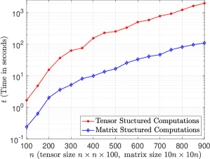
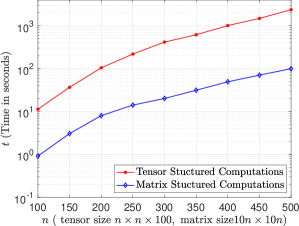
Note that the presented errors (Error and Error) and mean CPU times (MT and MT) for different sizes of and verifies the effectiveness of the algorithm in achieving accurate and efficient computations. The consistency in errors across different tensor and matrix dimensions demonstrates the robustness and reliability of the proposed approach.
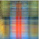
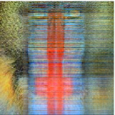
3.2 Lossy Image Compression
Image compression is essential in our increasingly data-driven world. The direct relationship between compressed image size and storage costs is significant. Further, compressed images require less bandwidth for transmission, which has several benefits, including reduced network congestion, lower energy consumption, and faster loading times for web pages and applications. Thus, the goal of compression is to minimize the number of bits needed to represent an image while maintaining acceptable quality. The challenge is finding the optimal balance between compression ratio and image quality. This subsection discusses lossy image compression based on decomposition. This decomposition represents an interesting approach to lossy compression that balances spatial and frequency domain considerations. Applications of lossy image compression are important in specific domains where its adaptive nature is particularly beneficial.


QDR decomposition of tensor often provides an attractive algebraic properties, i.e., a good balance between compression ratio and image quality. The color lossy image compression of a tensor can be written in the form of QDR decomposition.
where is the diagonal tensor, and is the upper triangular tensor. Here, the diagonal elements of decay rapidly, where . Further, QDR approximates this structure efficiently, concentrating most of the image information in the first columns or rows. The choice of determines the trade-off, i.e., larger represents better quality of image and lower compression, whereas smaller gives lower image quality with higher compression.


| Figure 4 | Figure 5 | ||||
|---|---|---|---|---|---|
| PSNR Value | SSIM Value | PSNR Value | SSIM Value | ||
| 50 | 10.15 | 0.6207 | 25 | 14.87 | 0.4089 |
| 100 | 12.84 | 0.7124 | 50 | 16.57 | 0.5567 |
| 150 | 17.21 | 0.8213 | 75 | 20.68 | 0.7573 |
| 200 | 21.65 | 0.8979 | 100 | 24.07 | 0.8512 |
| 150 | 26.84 | 0.9514 | 125 | 26.65 | 0.8972 |
| 300 | 30.27 | 0.9763 | 150 | 28.62 | 0.9250 |
| 350 | 33.65 | 0.9885 | 175 | 30.62 | 0.9445 |
| 400 | 37.95 | 0.9944 | 200 | 34.56 | 0.9720 |
| 450 | 45.08 | 0.9977 | 225 | 40.42 | 0.9908 |
| 500 | 61.62 | 0.9999 | 250 | 53.85 | 0.9994 |
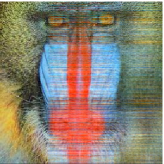
We present peak signal-to-noise ratio (PSNR) values in the Table 4 to assess image quality quantitatively for Figure 3. This calculation effectively compares the size of the error (represented by MSE) relative to the peak value of the signal max. Specifically, for color image of size is computed using the following
Here max is the maximum possible pixel value of the image (e.g., 255 for 8-bit images). Further, is the Mean Squared Error between the original and the processed images. See [3] for more detail. It is worth mentioning that the higher PSNR values correlate with superior image quality. PSNR is typically expressed in decibel units (dB). The values between 30-50 dB generally indicate acceptable to good image quality. However, PSNR exceeding 40 dB is considered to signify high-quality images where distortion is minimally perceptible to the human eye. In addition to this we also present another efficient tool for measuring image quality assessment for Figure 3 in the Table 4 i.e., structural similarity index (SSIM). SSIM is a perceptual metric that quantifies image quality degradation caused by processing such as data compression or by losses in data transmission. SSIM values range from to , where indicates perfect similarity between the original and processed images. See [3] for computational detail.
4 Computation of outer inverses via symbolic computation
Example 4.1.
Let with frontal slices are given by
Applying algorithm 4, we can compute the - decomposition of tensor , where and with respective frontal slices are given by
Next, we will discuss the computation of the outer inverse of tensors whose entries are either polynomial in single variable or rational functions, based on symbolic - decomposition. Consider with elements are
where is the maximal degrees of the numerators and and is the maximal degrees denominators of . Let the entries of and are in the following form
| (3) | |||||
| (4) |
Variables with an overbar represent the coefficients of the numerator, while variables with an underline represent the coefficients of the denominator, which can be followed subsequently. The representation of outer inverse of tensors over the field of rational functions is presented in the below theorem.
Theorem 4.2.
Proof.
In a special case, we can obtain the following representation for the Moore-Penrose inverse of tensors over the field of rational functions based on the - decomposition.
Theorem 4.3.
Let and with entries are of the form
Consider and be the - decomposition of , where the respective entries of and , are of the form
Assume that the entries of be of the form
| (8) |
Consider and . For and assume that
with degree . Then entries of are given by
where
, for each .
Since meromorphic functions are fractions of holomorphic functions, they can be extended as a nonzero polynomial in complex variables. We will compute from a random tensor whose entries are meromorphic functions, like , , , , where . More generally, when does not contain a holomorphic function, we can use Laurent formal power series to expand it as a truncated polynomial and can find the outer inverse of .
Example 4.4.
Consider two tensors and with frontal slices
and an invertible matrix . Approximate the tensor using the Laurent expansion up to four-degree terms.
Then, and . Then following Algorithm 5 one can compute as the following:
We compute as a special case in the following example.
5 Conclusion
The tensor forms of the FRD and --decomposition were developed based on the -product with powerful algorithms for their computations. The proposed --decomposition calculates the -Moore-Penrose inverse and outer inverse of a given third-order tensor whose entries are either symbolic (polynomial in a single variable) or rational. The proposed --decomposition is demonstrated by solving a few examples and applied to investigate lossy color image compression.
Data Availability Statement
The data that generated and support the findings of this study are available from the corresponding author upon reasonable request.
Conflict of Interest
The authors declare no potential conflict of interest.
Funding
-
1.
Ratikanta Behera is grateful for the support of the Anusandhan National Research Foundation (ANRF), Department of Science and Technology, India, under Grant No. EEQ/2022/001065.
-
2.
Jajati Keshari Sahoo is grateful for the support of the Anusandhan National Research Foundation (ANRF), Department of Science and Technology, India, under Grant No. SUR/2022/004357.
ORCID
Krushnachandra Panigrahy
https://orcid.org/0000-0003-0067-9298
Ratikanta Behera
https://orcid.org/0000-0002-6237-5700
Jajati Keshari Sahoo
https://orcid.org/0000-0001-6104-5171
Biswarup Karmakar
https://orcid.org/0009-0003-5635-5425
References
- [1] B. W. Bader and T. G. Kolda. Efficient MATLAB computations with sparse and factored tensors. SIAM J. Sci. Comput., 30(1):205–231, 2007/08.
- [2] R. Behera, J. K. Sahoo, R. N. Mohapatra, and M. Z. Nashed. Computation of generalized inverses of tensors via -product. Numer. Linear Algebra Appl., 29(2):Paper No. e2416, 24, 2022.
- [3] R. Behera, J. K. Sahoo, and Y. Wei. Computation of outer inverse of tensors based on -product. arXiv preprint arXiv:2311.17507, 2023.
- [4] K. Braman. Third-order tensors as linear operators on a space of matrices. Linear Algebra Appl., 433(7):1241–1253, 2010.
- [5] M. Brazell, N. Li, C. Navasca, and C. Tamon. Solving multilinear systems via tensor inversion. SIAM J. Matrix Anal. Appl., 34(2):542–570, 2013.
- [6] M. Che and Y. Wei. An efficient algorithm for computing the approximate t-URV and its applications. J. Sci. Comput., 92(3):Paper No. 93, 27, 2022.
- [7] A. Einstein. The foundation of the general theory of relativity. Annalen der Physik, 49(7):769–822, 1916.
- [8] N. Hao, M. E. Kilmer, K. Braman, and R. C. Hoover. Facial recognition using tensor-tensor decompositions. SIAM J. Imaging Sci., 6(1):437–463, 2013.
- [9] W. Hu, Y. Yang, W. Zhang, and Y. Xie. Moving object detection using tensor-based low-rank and saliently fused-sparse decomposition. IEEE Trans. Image Process., 26(2):724–737, 2017.
- [10] J. Ji and Y. Wei. The Drazin inverse of an even-order tensor and its application to singular tensor equations. Comput. Math. Appl., 75(9):3402–3413, 2018.
- [11] J. Ji and Y. Wei. The outer generalized inverse of an even-order tensor with the Einstein product through the matrix unfolding and tensor folding. Electron. J. Linear Algebra, 36:599–615, 2020.
- [12] H. Jin, S. Xu, Y. Wang, and X. Liu. The Moore-Penrose inverse of tensors via the M-product. Comput. Appl. Math., 42(6):Paper No. 294, 28, 2023.
- [13] E. Kernfeld, M. Kilmer, and S. Aeron. Tensor-tensor products with invertible linear transforms. Linear Algebra Appl., 485:545–570, 2015.
- [14] M. E. Kilmer, K. Braman, N. Hao, and R. C. Hoover. Third-order tensors as operators on matrices: a theoretical and computational framework with applications in imaging. SIAM J. Matrix Anal. Appl., 34(1):148–172, 2013.
- [15] M. E. Kilmer and C. D. Martin. Factorization strategies for third-order tensors. Linear Algebra Appl., 435(3):641–658, 2011.
- [16] T. G. Kolda and B. W. Bader. Tensor decompositions and applications. SIAM Rev., 51(3):455–500, 2009.
- [17] M. Liang and B. Zheng. Further results on Moore-Penrose inverses of tensors with application to tensor nearness problems. Comput. Math. Appl., 77(5):1282–1293, 2019.
- [18] Y. Liu, L. Chen, and C. Zhu. Improved robust tensor principal component analysis via low-rank core matrix. IEEE Journal of Selected Topics in Signal Processing, 12(6):1378–1389, 2018.
- [19] C. D. Martin, R. Shafer, and B. Larue. An order- tensor factorization with applications in imaging. SIAM J. Sci. Comput., 35(1):A474–A490, 2013.
- [20] L. Qi. Eigenvalues and invariants of tensors. J. Math. Anal. Appl., 325(2):1363–1377, 2007.
- [21] L. Qi and Z. Luo. Tensor analysis: Spectral theory and special tensors. Society for Industrial and Applied Mathematics, Philadelphia, PA, 2017.
- [22] J. K. Sahoo, R. Behera, P. S. Stanimirović, and V. N. Katsikis. Computation of outer inverses of tensors using the QR decomposition. Comput. Appl. Math., 39(3):Paper No. 199, 20, 2020.
- [23] J. K. Sahoo, S. K. Panda, R. Behera, and P. S. Stanimirović. Computation of tensors generalized inverses under -product and applications. arXiv preprint arXiv:2405.16111, 2024.
- [24] J.-Y. Shao. A general product of tensors with applications. Linear Algebra Appl., 439(8):2350–2366, 2013.
- [25] X. Sheng and G. Chen. Full-rank representation of generalized inverse and its application. Comput. Math. Appl., 54(11-12):1422–1430, 2007.
- [26] N. D. Sidiropoulos, L. De Lathauwer, X. Fu, K. Huang, E. E. Papalexakis, and C. Faloutsos. Tensor decomposition for signal processing and machine learning. IEEE Trans. Signal Process., 65(13):3551–3582, 2017.
- [27] S. Soltani, M. E. Kilmer, and P. C. Hansen. A tensor-based dictionary learning approach to tomographic image reconstruction. BIT Numer. Math., 56(4):1425–1454, 2016.
- [28] P. Soto-Quiros. Convergence analysis of iterative methods for computing the T-pseudoinverse of complete full-rank third-order tensors based on the T-product. Results Appl. Math., 18:Paper No. 100372, 7, 2023.
- [29] P. S. Stanimirović, D. Pappas, V. N. Katsikis, and I. P. Stanimirović. Symbolic computation of -inverses using factorization. Linear Algebra Appl., 437(6):1317–1331, 2012.
- [30] L. Sun, B. Zheng, C. Bu, and Y. Wei. Moore-Penrose inverse of tensors via Einstein product. Linear Multilinear Algebra, 64(4):686–698, 2016.
- [31] D. A. Tarzanagh and G. Michailidis. Fast randomized algorithms for t-product based tensor operations and decompositions with applications to imaging data. SIAM J. Imaging Sci., 11(4):2629–2664, 2018.