Applications of multiscale hierarchical decomposition to blind deconvolution
Abstract
The blind image deconvolution is a challenging, highly ill-posed nonlinear inverse problem. We introduce a Multiscale Hierarchical Decomposition Method (MHDM) that is iteratively solving variational problems with adaptive data and regularization parameters, towards obtaining finer and finer details of the unknown kernel and image. We establish convergence of the residual in the noise-free data case, and then in the noisy data case when the algorithm is stopped early by means of a discrepancy principle. Fractional Sobolev norms are employed as regularizers for both kernel and image, with the advantage of computing the minimizers explicitly in a pointwise manner. In order to break the notorious symmetry occurring during each minimization step, we enforce a positivity constraint on the Fourier transform of the kernels. Numerical comparisons with a single-step variational method and a non-blind MHDM show that our approach produces comparable results, while less laborious parameter tuning is necessary at the price of more computations. Additionally, the scale decomposition of both reconstructed kernel and image provides a meaningful interpretation of the involved iteration steps.
1 Introduction
An important problem in image processing is the image restoration one, which aims to remove noise and blur from a degraded image. More precisely, assume that is a given blurry-noisy image, with the degradation model where is the true image to be recovered, is a blurring kernel, and denotes some kind of additive noise. There are plenty of statistical, variational and partial differential equation strategies to approach the problem. A classical variational model for this linear ill-posed problem under the assumption of normally distributed noise is
| (1) |
where is the regularization parameter that should balance stability and accuracy in the solution reconstruction, and stands for a penalty that promotes desired features for the recovered image, such as total variation in case of piecewise constant structures (see [31]). However, recovering both and from , knowing little information about the degradation, is a highly ill-posed nonlinear inverse problem, so-called blind deconvolution. For instance, it occurs in the context of astronomical imaging [16, 26, 29], microscopy [18, 9, 38] or movement correction in digital photography [6, 12, 21]. As above, one way to alleviate the difficulty in solving this problem is to use the variational approach with regularization.
Seminal work in [37] and [8] proposed blind deconvolution models using joint minimizations of the form
| (2) |
which can be solved using alternating minimization and two coupled Euler-Lagrange equations. Here denotes some generic regularization functional, which might be chosen differently for and . In [37], the regularization terms were both Sobolev norms, while in [8], they were the total variation for , and total variation or the Sobolev norm for . Still, the joint regularization problem, as is, involves too much symmetry between the unknowns and and thus, non-uniqueness issues appear. Note that, under some assumptions, if is a joint minimizer in (2), then also is a joint minimizer, for some constant . A detailed analysis of this difficulty and useful ideas are presented in the book [7, Chapter 5]. For instance, additional constraints can be included for better restoration: , , or radially symmetric, to break the symmetry of the problem. Regarding possible regularization functionals, we mention the works [36, 33, 20] which employ sparsity promoting functionals based on (quasi)norms, as well as [11, 32] where generalizations of the total variation are used as penalty terms for the image. Note that regularization of both the image and the kernel seems necessary, since omitting a penalty on the latter might lead to inadequate results, cf [27]. Beside the variational approaches, two stage methods [10, 17], as well as a multitude of (statistically motivated) iterative algorithms [15, 23, 13, 1, 22] have been proposed. More recently, the application of machine learning methods to blind deconvolution has become popular [30, 3, 14]. However, in this work, we focus on a different technique, called multiscale hierarchical decomposition of images (MHDM), introduced in [34, 35], that favors gradual reconstruction of image features at increasingly small scales. More precisely, in that work for (denoising and) non-blind deconvolution, it was emphasized that separating cartoon and texture in images is highly dependent on the scale from (1), in the sense that details in an image (usually part of the texture) can be seen as a cartoon at a refined scale, such as .
In [34, 35], one starts with getting a minimizer of (1), then continues with iteratively solving similar minimization problems which aim at extracting more detailed information from the current data by using different scale parameters at every step. Thus, one obtains a sequence of minimizers , , …, via
such that . Energy estimates and applications to non-blind deconvolution, scale separation, and registration are shown in [35, 25]. Moreover, error estimates for the data-fitting term, and stopping index rules are provided in recent works [24, 19, 2], which also clearly point out that the MHDM merits are at least twofold. Namely, it provides fine recoveries of images with multiscale features that are otherwise not obtainable by single step variational models, and it is pretty robust with respect to the choice of the initial parameter (and of parameters involved in the computational procedures), thus avoiding the burden of choosing it appropriately when performing only one step in (1). To be fair though on the comparison, note that more computations are involved when using MHDM.
To benefit from these effects, we are interested to extend the MHDM to the more complex problem of blind deconvolution. Clearly, we do not have
as we would try to “blindly” apply the hierarchical decomposition method to blind deconvolution. Instead, we introduce an appropriate procedure that provides reconstructions of the kernel and of the true image of the form in the left-hand side above. Let us first specify the notation. We consider the observed blurred and noisy image given by
| (3) |
where is the true image, a blurring kernel, and some additive noise. Here, the convolution has to be understood in the following sense: Let be a bounded Lipschitz domain that contains the support of and . Then the convolution is performed by extending with outside and considering only the restriction of to . Let and be proper, lower semicontinuous, convex and non-negative functionals. The aim is to reconstruct and from the observation by adapting the MHDM to problem (3). That is, we would like to decompose and as sums
| (4) |
where each component and contains features of and , respectively, at a different scale. Therefore, we proceed as follows. Let be decreasing sequences of positive real numbers. Additionally, let be a measure of similarity between and an image , which satisfies for all with . We consider data fidelity terms for noisy observations that have the form
| (5) |
Here
denotes the indicator function of a convex set and is used to encode additional assumptions such as positivity of the kernel or constraints on the means of images and kernels.
We compute the initial iterates as
| (6) |
Next, set , and determine the increments such that and via
Thus, we iterate for ,
| (7) |
that is,
and set , . Note that (7) can also be formulated as
| (8) |
We extract in a nonlinear way a sequence of functions (atoms) approximating ,
This refined multiscale hierarchical blind deconvolution model will provide a better choice for the solution than the single step (variational) model, especially when reconstructing images with different scales, as each component at a scale contains additional information that would have been ignored at the previous, coarser scales. As usual for ill-posed problems, we stop the iterations early, according to the discrepancy principle, in order to prevent meaningless computational steps.
We focus on Sobolev norms as regularizers for both kernel and image, and show that the iterates can be computed in a pointwise manner by means of the Fourier domain. When choosing the Fourier transforms of the kernels to be positive, we get the chance to break the unwanted symmetry which naturally occurs in such regularization frameworks. An interpretation of this choice in terms of positive definite functions is provided as well. Note that considering more modern penalties in our approach is beyond the scope of this study, since it would require accounting for a priori information and tedious computational methods specific to that setting.
Our work is structured as follows. Section 2 presents the convergence properties of the method, as well as the stopping rule. Section 3 is dedicated to the regularization with Sobolev norms, detailing the pointwise computation of the minimizers, while Section 4 illustrates the numerical experiments that fairly compare our procedure to a single-step variational method and to a non-blind deconvolution method.
2 Convergence properties and stopping rule
To the best of our knowledge, convergence results of the iterates and generated by the MHDM are not even known for simpler one-variable deblurring problems, see [35]. However, convergence of the residual can be shown analogously to Theorem 2.1 in [19]. For completeness, we will provide the proof in the case of noise free data.
Theorem 2.1.
It is well-known that iterative methods for ill-posed problems perturbed by noise have to be stopped early. We use the discrepancy principle as a stopping criterion, namely we terminate the iteration at index defined as
| (13) |
for some . The well-definedness of the stopping index is a consequence of the following Theorem, where for simplicity of notation the iterates obtained from the noisy observation are still denoted by and .
3 Sobolev norm regularizers
In order to illustrate our proposed method, we follow the work [5] and use Sobolev norms as regularizers for kernels and images. That is, we consider the case , , and for . For defining the Bessel Potential norm for we set . Then
| (15) |
where is the Fourier transform of extended by zero outside of . Note that the well-definedness of the MHDM with those regularizers follows analogously to [17, Theorem 3.6] for all sets of constraints satisfying and . However, we will start with analyzing the MHDM without any constraints (i.e. ). Hence, we compute the first iterate via
| (16) |
The norm defined in (15) is a different, but equivalent norm than the one used in [5]. Nonetheless, the results of [5, Lemma 3.3] still hold: Denote the Fourier transform of by and the complex conjugate of a complex number . Then, the Fourier transforms of all minimizers of (16) are pointwise given as
| (17) | |||
| (18) |
for arbitrary measurable functions with for all . Here .
For our method, we choose and compute by applying the inverse Fourier transform. In particular, this means that the Fourier transform of is non-negative almost everywhere. Let us give an interpretation of this. First, recall the notion of positive definite functions (see, e.g. [28, Section 4.4.3]).
Definition 3.1.
A function is positive semi-definite if it satisfies
| (19) |
for all , and any .
Lemma 3.2.
Let be a function such that its Fourier transform is non-negative almost everywhere. Then is positive semi-definite.
Proof.
It follows analogously to the proof of [28, Theorem 4.89]. ∎
This means, the kernel obtained from choosing in (18) is positive semi-definite. In particular, it has the following properties, as one can see from (19).
Corollary 3.3.
Let be positive semi-definite. Then
-
(i)
,
-
(ii)
for all ,
-
(iii)
for all .
Thus, attains a maximum at . Additionally, as a solution of (6), it is real-valued and satisfies for all . Therefore, the solutions of (16) will be even functions with a peak at , so that they might be particularly useful to approximate conical combinations of centered Gaussians. We therefore want to have the constraint of the kernels having non-negative Fourier-transforms for all iterates of the MHDM. As the following will show, the iterates of the MHDM with can be chosen to have this property. The advantage is that we can derive an explicit way to compute the iterates pointwise as certain minimizers of the unconstrained problems. Let us start with explaining how to compute the increments for . We have to solve problems of the form
| (20) |
Thus, in the Fourier space, this amounts to solving
| (21) |
Following the notation of [5], we fix and set
| (22) |
Hence, we are concerned with computing
| (23) |
where and .
The following Theorem shows that it is possible to choose the increment non-negative for all , which therefore yields that the iterates are non-negative, for all .
Theorem 3.4.
There is a choice for such that
-
(i)
,
-
(ii)
,
-
(iii)
for all . Here and are understood as the solution of (23) with .
Proof.
If , then for all , and the claim follows trivially. Hence, we assume . First, note that for any , the first order optimality condition of (23) implies
| (24) | |||
| (25) |
for any pair minimizing . Since for all , equation (24) is equivalent to
| (26) |
With this, we can prove the claims by induction.
- Base case:
- Induction step:
-
Assume – hold for some . In particular, this means , so that (26) becomes
(27) Hence, we can restrict the minimization of to minimizing over the set of all , for which satisfies (27). We thus need to minimize the functional
-
()
In order to show that , we only need to show that we can choose . First, observe that must attain a minimum by coercivity and continuity. Therefore, let be a minimizer of . Hence, it suffices to prove . Let now . We show that on the set , the choice minimizes . Indeed, for with , it holds
where the last inequality follows from and . Thus, for any the minimum of on the circle of radius is attained for . In particular, we obtain .
-
()
From the previous part, we know that there is a pair minimizing such that . By definition, it is , so we can multiply (27) with to obtain
-
()
If , the claim follows trivially. Thus, we assume and find from (25) that
Multiplying with and rearranging implies
Denote and . It is
since . Therefore, , which yields .
-
()
∎
We can use the previous theorem to construct a method to directly solve (23). First, we plug (27) in (25) to obtain
Multiplying with , we get
| (28) |
Since we are interested in finding a real solution of this equation, we can assume and expand to
| (29) |
Since both and are real numbers, this is a polynomial of degree with only real coefficients. We can thus choose to be the real root of (3), for which attains the smallest value. Thus, by choosing the minimizers for which the Fourier transform of the kernel is real and non-negative in the MHDM iteration, we can implicitly incorporate the constraint for all . Therefore, all approximations of the kernel will be positive semi-definite enforcing properties – in Corollary 3.3, that acts as a way to break the symmetry of problem (16).
Remark.
If more information on the phase of the true kernel is available, one might want to one choose in (17) and (18) to be a different complex-valued function instead of a non-negative one. In this case, the sequence generated by (21) can be chosen such that for all . To see this, notice that substituting , , and for , , and , respectively, in (21), does not change the value of the objective function. Thus, we can use the iterates obtained with the constraint to compute the iterates of a MHDM with the constraint .
In order to further ensure that the iterates are reasonable approximations of the true image and kernel, we additionally impose constraints on their means:
| (30) |
for all . Those constraints are fairly standard and can for instance be found in [7, 15]. In summary, this means we are considering the constraint sets:
It is not clear if these constraints can be translated into Fourier space such that the iterates of the MHDM can still be computed in a pointwise manner. Since for any function with and it is known that is uniformly continuous [4], it must be . However, simply enforcing the constraint in (21) does not affect as the resulting minimizer in Fourier space would only differ from the unconstrained one on a set of measure . Note that this problem does not arise in the discretized setting we use for the numerical experiments, as will be outlined later.
Remark.
Instead of employing a Bessel Potential norm as a penalty term for the image, it would be a natural idea to use a functional that favors expected structures. For instance, one could use the total variation to promote cartoon-like images. However, numerical experiments suggest that the iterates of such MHDM seem to approximate the trivial solution and , where denotes the Dirac delta distribution. This could possibly be overcome by a specific choice for the sequences and , but would first require a deeper analysis of convergence behavior of the blind MHDM in this scenario, which is not within the scope of this work.
4 Numerical Experiments
The goal of our numerical experiments is to illustrate the behavior and robustness of the blind deconvolution MHDM. To this end, we compare the reconstructed image and kernel from the proposed method to those obtained from using a non-blind MHDM or a single step variational regularization, as in (16). To achieve a fair comparison, we use the same regularizers for all methods under investigation. By using squared Bessel Potential norms, we obtain reasonable reconstructions that might not necessarily outperform methods with more problem specific regularizers. However, we think that comparing our approach to such methods should be done with a version of the MHDM that also uses more sophisticated regularizers, that is beyond the scope of this work. We want to stress that the advantage of our method is the interpretability of the scale decomposition and the potential to adapt it to a multitude of regularizers that possibly could vary along the iterations.
4.1 Discretization and Implementation
Recall that and for . We discretize an image on a rectangular domain as a matrix, i.e., . Following the derivation in Section 7.1.2 of [17], we define the weight matrix for the Sobolev norm in Fourier space by the matrix with entries
Hence, a discretization of the Sobolev norm is given by
where denotes the discrete Fourier transform. Therefore, the -th step of the MHDM is given by the pointwise update rule
| (31) |
Thus for , we can solve (31) by
For , make the corresponding substitutions as in (3):
To find critical pairs , we compute the positive roots of (3) that yield candidates for and use (27) to obtain the corresponding candidates for . The minimizing pair can then be found by choosing the critical pair, which gives the smallest value for the objective function in (31). In order to obtain meaningful reconstructions , we employ the additional constraint (30) that the mean of the kernel is and the mean of the reconstructed image matches the mean of the observation. In the discretization that means
Since we are using discrete Fourier transforms, these constraints are equivalent to and . Thus, we implement them by making the updates
instead of the previous procedure for the first entries of the matrices.
4.2 Experiment 1: Performance of blind MHDM
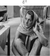
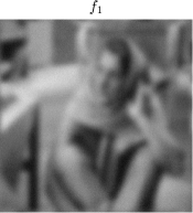
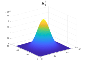
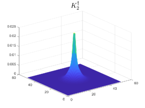
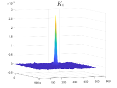
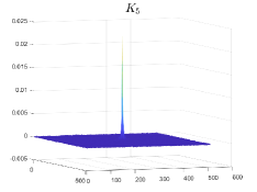
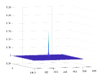
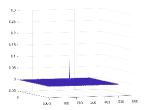
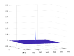
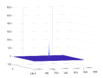
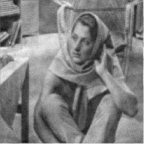
We test the algorithm on the image Barbara (denoted by ), which has been blurred by convolution with two different kernels. For the first blurring we choose a Gaussian kernel of mean and variance . In the second kernel , we use a convex combination of several Gaussians. In both cases, the blurred image was additionally corrupted with additive Gaussian noise (mean , variance ). That is, we deal with observations obtained via for . The true image, blurred images and noise corrupted blurred images can be found in Figure 1, the corresponding kernels are shown in Figure 2.

Curiously, the results of our experiments improve if is chosen smaller than . This means, we penalize the image with a more smoothness promoting regularizer than the kernel. Furthermore, we point out that as long as the ratio is constant, the actual choice of the initial parameters does not significantly influence the quality of the final iterates but only the number of iterations needed until the discrepancy principle is satisfied. This poses an advantage over single-step variational methods, as the proposed method only requires a choice of the ratio of the initial parameters, instead of both parameters and . For our experiments we choose and , and run the MHDM with initial parameters , . In accordance with Theorem 2.2, we choose the parameters at the -th step as and . Since in this experiment we artificially added noise and hence know the exact noise level, the iteration is stopped according to the discrepancy principle (13) with .
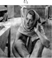
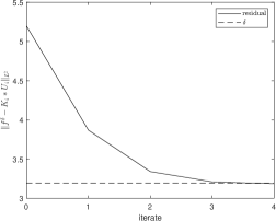
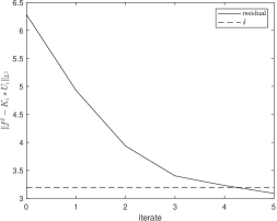
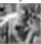
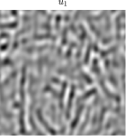
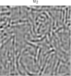
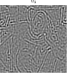
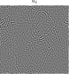
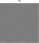
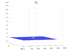
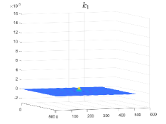
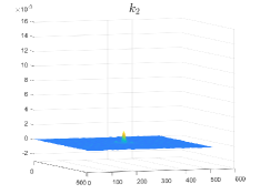
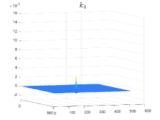
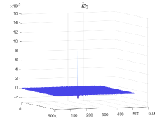
Figure 4 shows the decay of the residual for both experiments. In both figures, one can clearly see the monotone decrease of the residual, confirming the theoretical results from Theorem 2.1. Figure 5 shows the different scales that are obtained with the MHDM employed for the observation . One can see that each step adds another layer of details to the reconstruction. The corresponding scales for the reconstructed kernel can be seen in Figure 2. It appears that the role of the scales is to adapt the reconstructed kernel in a twofold way. On the one side, the height of the peak seems to be increased, while its radius decreases. On the other side, the plateau around the peak seems to be smoothened. Notably, the early coarse scales seem to recover the general shape and radius of the bump and the fine scales mostly shape the height of it. In the experiment with data , the scale decomposition for the reconstructed image and kernel look similar.


Moreover, we observe that a suboptimal choice for the initial ratio leads to a worse kernel reconstruction while, upon an affine rescaling of the grayscale values, the reconstructed images are visually still good. This is illustrated in Figure 7, where the reconstructed kernels and images (with the pixel values rescaled) for different initial parameters and are shown. We observe that visually all images are indistinguishable and approximate the true image well. Similarly, the corresponding kernels are structurally similar to the real one, but their numerical values are very disproportional.


4.3 Experiment 2: Comparison of blind MHDM vs. non-blind MHDM
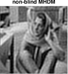
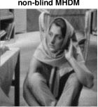
We compare the proposed blind MHDM to a non-blind version of the MHDM (see for instance [35, 24]) that uses the penalty term for the image. Instead of including the reconstruction of the blurring kernel in the method, we simply make a guess in the non-blind MHDM and stop the iteration once the discrepancy principle is satisfied. The non-blind MHDM therefore only requires the choice of one initial parameter , which we choose to be the same as for the blind deconvolution MHDM and also decrease according to the rule . To compare the two methods, we test the non-blind MHDM for centered Gaussian kernels with variances ranging between and as guessed kernels.
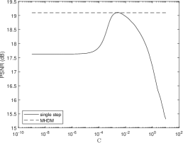
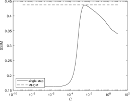
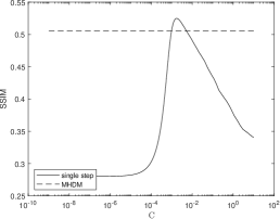
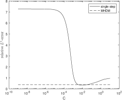
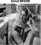
In Figures 8 and 9, we compare the performance of the blind MHDM with the non-blind MHDM algorithm in terms of the error measures PSNR, SSIM (Figure 8), and the -error of the kernel (Figure 9). We consider either the data (figures on the left-hand side) or (figures on the right-hand side). In each of the plots, the values on the -axis correspond to the guessed variance of the Gaussian kernel used for the non-blind MHDM. The full line corresponds to the values of the resulting respective error measures, whereas the constant dashed line represents the value of the blind MHDM. Clearly, the quality of the non-blind algorithms depends on the correctness of the choice of . For the observation , which corresponds to blurring with a single Gaussian kernel, the non-blind MHDM expectedly outperforms the blind MHDM only for kernel guesses that are similar to the true kernel. We observe similar behavior for the case with multiple Gaussian kernels used in the blurring. However, let us point out that, especially for the error measures PSNR and SSIM, the non-blind method has only a rather modest advantage and only in the case when the “guessed” is close to the true one, while in case of a wrong guess, the non-blind method can go wrong quite dramatically as can be seen from the experiments with observation (the bottom line in Figure 8). These result indicate that the blind MHDM is a robust method that produces reasonable results without the need of knowledge of In particular, if the blurring kernel cannot be estimated with high accuracy, then the blind MHDM is superior to non-blind approaches.


Top right: SSIM values for MHDM with guessed kernel for different guesses of the kernel and data ,
Bottom left: PSNR values for MHDM with guessed kernel for different guesses of the kernel and data ,
Bottom right: SSIM values for MHDM with guessed kernel for different guesses of the kernel and data .

4.4 Experiment 3: Comparison blind MHDM vs variational blind deconvolution
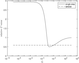
Next, we compare the MHDM to the single step variational method (16). Since according to Theorem 3.4 in [5], the only condition for convergence of the single-step regularized approximations to a solution of is that the parameters converge to as , we have no a priori knowledge on an optimal choice of the regularization parameters and . We therefore test the single-step methods with parameters that have the same ratio as the ones used for the MHDM. That is, for given we choose and , where and are the initial parameters of the blind MHDM. We test the non-blind method for logarithmically spaced values of ranging from to .
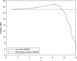
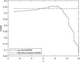
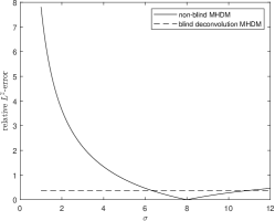
Figure 10 compares the PSNR and SSIM values of the images reconstructed with a single iteration (i.e., variational regularization) versus the blind MHDM for both observations and . The -axis depicts the parameter with which and were multiplied in the single step method. The corresponding relative errors of the reconstructed kernels can be seen in Figure 11. As previously, the constant dashed line represents the respective values of the blind MHDM, which are obtained by using the initial parameters , and hence, do not depend on , while the full line depicts the values of the single step method for given .
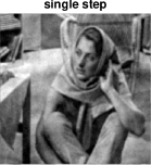
We observe that in the first experiment with data (i.e., blurring with a single Gaussian kernel), the single step method outperforms the MHDM in PSNR only for factors in the range between and , while the SSIM obtained by the blind MHDM is better for any value of . Moreover, this outperformance is relatively small and visually hardly recognizable, as can be seen in Figure 12. The relative -error of the kernels obtained by the single step method was at best about of the error of the blind kernel. In the case of data , the single step method outperforms the MHDM in PSNR only for values of ranging from to and in SSIM only for between and . Hence, we argue that the blind MHDM mostly performs better than the single step method. In order to actually obtain better results than the MHDM, extensive parameter tuning in the single step method is required. Additionally, the initial parameters for the MHDM are not chosen optimal, so that the best possible single step performance might also be matched by the MHDM with an improved parameter choice.

Top right: SSIM values for MHDM with guessed kernel for different parameter choices , and data ,
Bottom left: PSNR values for MHDM with guessed kernel for different parameter choices , and data ,
Bottom right: SSIM values for MHDM with guessed kernel for different parameter choices , and data .


5 Conclusion
We introduce the Multiscale Hierarchical Decomposition Method for the blind deconvolution problem and show convergence of the residual in the noise-free case and then in the noisy data case, by employing a discrepancy principle. To demonstrate the efficiency and behavior of the proposed method, we focus on employing fractional Sobolev norms as regularizers, and develop a way to compute the appearing minimizers explicitly in a pointwise manner. We want to stress that in our experience, any variational approach to blind deconvolution should incorporate prior information on the expected blurring kernel. In our setting, this was done by enforcing a positivity constraint on the Fourier transform of the kernels, thus favoring, e.g., Gaussian structures. Numerical comparisons with a single-step variational method and a non-blind MHDM show that our approach produces comparable results, while fewer laborious parameter tuning is necessary. Additionally, the scale decomposition of both reconstructed kernel and image provides a meaningful interpretation of the involved iteration steps. For future work, this opens up the possibility to modify the method based on prior information of the underlying true solution. By using multiple penalty terms throughout the iteration, one could construct approximate solutions that admit different structures at different levels of detail. Nonetheless, we believe that at first a better understanding of iterates’ convergence behavior is necessary to systematically refine the method.
6 Acknowledgements
We thank Michael Quellmalz (Technische Universität Berlin) for his remarks and literature suggestion on the positivity of Fourier transforms. This research was funded in part by the Austrian Science Fund (FWF) [10.55776/DOC78]. For open access purposes, the authors have applied a CC BY public copyright license to any author-accepted manuscript version arising from this submission.
References
- [1] S. D. Babacan, R. Molina, and A. K. Katsaggelos. Variational bayesian blind deconvolution using a total variation prior. IEEE Transactions on Image Processing, 18(1):12–26, 2009.
- [2] J. Barnett, W. Li, E. Resmerita, and L. Vese. Multiscale hierarchical decomposition methods for images corrupted by multiplicative noise. arXiv preprint arXiv:2310.06195, 2023.
- [3] A. Benfenati, A. Catozzi, and V. Ruggiero. Neural blind deconvolution with poisson data. Inverse Problems, 39(5):054003, mar 2023.
- [4] S. Bochner and K. Chandrasekharan. Fourier Transforms. Annals of Mathematics Studies. Princeton University Press, 1949.
- [5] M. Burger and O. Scherzer. Regularization methods for blind deconvolution and blind source separation problems. Mathematics of Control, Signals and Systems, 14:358–383, 2001.
- [6] J.-F. Cai, H. Ji, C. Liu, and Z. Shen. Blind motion deblurring using multiple images. Journal of Computational Physics, 228(14):5057–5071, 2009.
- [7] T. F. Chan and J. Shen. Image processing and analysis: variational, PDE, wavelet, and stochastic methods. SIAM, 2005.
- [8] T. F. Chan and C.-K. Wong. Total variation blind deconvolution. IEEE transactions on Image Processing, 7(3):370–375, 1998.
- [9] J. Chen, R. Lin, H. Wang, J. Meng, H. Zheng, and L. Song. Blind-deconvolution optical-resolution photoacoustic microscopy in vivo. Optics Express, 21:7316–27, 03 2013.
- [10] M. Delbracio, I. Garcia-Dorado, S. Choi, D. Kelly, and P. Milanfar. Polyblur: Removing mild blur by polynomial reblurring. IEEE Transactions on Computational Imaging, PP:1–1, 07 2021.
- [11] I. El Mourabit, M. El Rhabi, and A. Hakim. Blind deconvolution using bilateral total variation regularization: a theoretical study and application. Applicable Analysis, 101(16):5660–5673, 2022.
- [12] R. Fergus, B. Singh, A. Hertzmann, S. T. Roweis, and W. T. Freeman. Removing camera shake from a single photograph. ACM SIGGRAPH 2006 Papers, 2006.
- [13] D. A. Fish, A. M. Brinicombe, E. R. Pike, and J. G. Walker. Blind deconvolution by means of the richardson–lucy algorithm. J. Opt. Soc. Am. A, 12(1):58–65, Jan 1995.
- [14] A. Gossard and P. Weiss. Training adaptive reconstruction networks for blind inverse problems. SIAM Journal on Imaging Sciences, 17(2):1314–1346, 2024.
- [15] L. He, A. Marquina, and S. J. Osher. Blind deconvolution using TV regularization and bregman iteration. Int. J. Imaging Syst. Technol., 15(1):74–83, 2005.
- [16] S. Jefferies and J. Christou. Restoration of astronomical images by iterative blind deconvolution. The Astrophysical Journal, 415:862, 09 1993.
- [17] L. Justen. Blind Deconvolution: Theory, Regularization and Applications. Industriemathematik und Angewandte Mathematik. Shaker, 2006.
- [18] K. Kim and J.-Y. Kim. Blind deconvolution based on compressed sensing with bi-l0-l2-norm regularization in light microscopy image. International Journal of Environmental Research and Public Health, 18:1789, 02 2021.
- [19] S. Kindermann, E. Resmerita, and T. Wolf. Multiscale hierarchical decomposition methods for ill-posed problems. Inverse Problems, 39(12):125013, 2023.
- [20] D. Krishnan, T. Tay, and R. Fergus. Blind deconvolution using a normalized sparsity measure. In Proceedings of the IEEE Computer Society Conference on Computer Vision and Pattern Recognition, pages 233 – 240, 07 2011.
- [21] A. Levin. Blind motion deblurring using image statistics. In Neural Information Processing Systems (NIPS), volume 19, pages 841–848, 01 2006.
- [22] A. Levin, Y. Weiss, F. Durand, and W. Freeman. Understanding and evaluating blind deconvolution algorithms. 2012 IEEE Conference on Computer Vision and Pattern Recognition, 0:1964–1971, 06 2009.
- [23] W. Li, Q. Li, W. Gong, and S. Tang. Total variation blind deconvolution employing split bregman iteration. Journal of Visual Communication and Image Representation, 23(3):409–417, 2012.
- [24] W. Li, E. Resmerita, and L. A. Vese. Multiscale hierarchical image decomposition and refinements: Qualitative and quantitative results. SIAM Journal on Imaging Sciences, 14(2):844–877, 2021.
- [25] K. Modin, A. Nachman, and L. Rondi. A multiscale theory for image registration and nonlinear inverse problems. Advances in Mathematics, 346:1009–1066, 2019.
- [26] E. Pantin, J.-L. Starck, and F. Murtagh. Deconvolution and Blind Deconvolution in Astronomy, pages 277–316. CRC Press, 05 2007.
- [27] D. Perrone and P. Favaro. Total variation blind deconvolution: The devil is in the details. In 2014 IEEE Conference on Computer Vision and Pattern Recognition, pages 2909–2916, 2014.
- [28] G. Plonka, D. Potts, G. Steidl, and M. Tasche. Numerical Fourier Analysis -. Springer Nature, Singapore, second edition, 2023.
- [29] M. Prato, A. L. Camera, S. Bonettini, and M. Bertero. A convergent blind deconvolution method for post-adaptive-optics astronomical imaging. Inverse Problems, 29(6):065017, may 2013.
- [30] D. Ren, K. Zhang, Q. Wang, Q. Hu, and W. Zuo. Neural blind deconvolution using deep priors. In Proceedings of the IEEE/CVF conference on computer vision and pattern recognition, pages 3341–3350, 2020.
- [31] L. I. Rudin, S. Osher, and E. Fatemi. Nonlinear total variation based noise removal algorithms. Physica D: nonlinear phenomena, 60(1-4):259–268, 1992.
- [32] W. Shao, F. Wang, and L.-L. Huang. Adapting total generalized variation for blind image restoration. Multidimensional Systems and Signal Processing, 30, 04 2019.
- [33] W.-Z. Shao, H.-B. Li, and M. Elad. Bi-l0-l2-norm regularization for blind motion deblurring. Journal of Visual Communication and Image Representation, 33:42–59, 2015.
- [34] E. Tadmor, S. Nezzar, and L. Vese. A multiscale image representation using hierarchical (BV,) decompositions. Multiscale Modeling & Simulation, 2:554–579, 2004.
- [35] E. Tadmor, S. Nezzar, and L. Vese. Multiscale hierarchical decomposition of images with applications to deblurring, denoising and segmentation. Commun. Math. Sci., 6:281–307, 2008.
- [36] W. Wang, J. Li, and H. Ji. -norm regularization for short-and-sparse blind deconvolution: Point source separability and region selection. SIAM Journal on Imaging Sciences, 15:1345–1372, 09 2022.
- [37] Y.-L. You and M. Kaveh. A regularization approach to joint blur identification and image restoration. IEEE Transactions on Image Processing, 5(3):416–428, 1996.
- [38] F. Ávila and J. Bueno. Spherical aberration and scattering compensation in microscopy images through a blind deconvolution method. Journal of Imaging, 10:43, 02 2024.