Mean square displacement of intruders in freely cooling multicomponent granular mixtures

Abstract

The mean square displacement (MSD) of intruders (tracer particles) immersed in a multicomponent granular mixture made up of smooth inelastic hard spheres in a homogeneous cooling state is explicitly computed. The multicomponent granular mixture is constituted by $s$ species with different masses, diameters, and coefficients of restitution. In the hydrodynamic regime, the time decay of the granular temperature of the mixture gives rise to a time decay of the intruder’s diffusion coefficient $D_{0}$. The corresponding MSD of the intruder is determined by integrating the corresponding diffusion equation. As expected from previous works on binary mixtures, we find a logarithmic time dependence of the MSD which involves the coefficient $D_{0}$. To analyze the dependence of the MSD on the parameter space of the system, the diffusion coefficient is explicitly determined by considering the so-called second Sonine approximation (two terms in the Sonine polynomial expansion of the intruder’s distribution function). The theoretical results for $D_{0}$ are compared with those obtained by numerically solving the Boltzmann equation by means of the direct simulation Monte Carlo method. We show that the second Sonine approximation improves the predictions of the first Sonine approximation, especially when the intruders are much lighter than the particles of the granular mixture. In the long-time limit, our results for the MSD agree with those recently obtained by Bodrova [Phys. Rev. E 109, 024903 (2024)] when $D_{0}$ is determined by considering the first Sonine approximation.

I Introduction

Granular materials in both nature and industry are usually characterized by some degree of polydispersity in both mass density and size. Due to the differences in mass and/or size of particles of each species, multicomponent mixtures exhibit particle segregation or demixing Ottino and Khakhar (2000); Kudrolli (2004). Thus, the study of transport properties in multicomponent granular mixtures is relevant not only from a fundamental point of view but also from a practical perspective.

When granular matter is subjected to an external excitation, the energy input supplied to the grains can compensate for the energy dissipated through collisions. In this situation, the motion of grains is quite similar to the chaotic motion of atoms or molecules in a conventional fluid. In this regime (referred to as rapid flow conditions), the collisions of grains play a relevant role in their dynamics and hence, kinetic theory tools (conveniently adapted to take into account the dissipative character of collisions) have been employed in the last few years Goldhirsch (2003); Brilliantov and Pöschel (2004); Garzó (2019) to analyze granular flows. In particular, for sufficiently dilute systems, granular materials can be modeled as a gas of smooth inelastic hard spheres where the inelasticity of collisions is only characterized by a constant coefficient of normal restitution.

The fact that the collisions between grains are inelastic implies that their diffusive motion will eventually stop in the absence of an external excitation. For this reason, most of the studies of diffusion in granular systems have been carried out in driven steady states Ippolito et al. (1995); S. and Urbach (1999); Wildman et al. (2001); Melby et al. (2005); Gómez González et al. (2023). However, diffusion can also be studied in freely cooling systems, specifically in the homogeneous cooling state (HCS). The detailed analysis of diffusive transport in the HCS for multicomponent granular mixtures can be considered as an important goal with some as yet open questions. For example, understanding how variations in particle sizes affect diffusion is crucial for optimizing pharmaceutical mixers.

To the best of our knowledge, the first works on the diffusion of an intruder in a freely cooling granular gas were focused on two limiting cases: (i) the self-diffusion problem (intruder is mechanically equivalent to the particles of the granular gas) Brey et al. (2000); Brilliantov and Pöschel (2000); Bodrova et al. (2015a) and the Brownian limit (intruder is much heavier than the particles of the granular gas) Brey et al. (1999); Sarracino et al. (2010). In both limiting cases, Haff’s law Haff (1983) for the granular temperature yields a diffusion coefficient that decays in time. This dependence gives rise to a logarithmic time dependence of the MSD of intruder. A more recent study has extended these previous findings to arbitrary values of the intruder-grain mass ratio Abad et al. (2022).

All previous works Brey et al. (2000); Brilliantov and Pöschel (2000); Bodrova et al. (2015a); Brey et al. (1999); Sarracino et al. (2010); Abad et al. (2022) refer to the diffusion of the intruder in a granular gas. However, studies on intruder diffusion in multicomponent or polydisperse granular systems are much scarcer. We are aware of only a very recent work Bodrova (2024) where the MSD of granular particles in a multicomponent granular mixture (containing an arbitrary number of species with different masses and diameters) under HCS has been explicitly determined. Although this work fills an important gap in the granular literature, the results derived in Ref. Bodrova (2024) are based on a simplifying assumption that was not explicitly stated in the paper: the MSD of species $k$ was determined by considering the so-called first Sonine approximation to the partial diffusion coefficient $D_{k}$. However, as has been clearly shown in previous works on binary granular mixtures Garzó and Montanero (2004); Garzó and Vega Reyes (2009, 2012); Garzó et al. (2013); Gómez González and Garzó (2023, 2024), the first Sonine approximation to $D_{k}$ exhibits significant deviations from computer simulation data when the intruder is much lighter than the particles of the granular gas. These differences are clearly mitigated when considering the next correction to $D_{k}$, namely the second Sonine approximation to $D_{k}$. The question then arises as to whether and if so to what extent, the conclusions drawn from Ref. Bodrova (2024) may change when the second Sonine correction to $D_{k}$ is accounted for in the theory.

In this paper, we address the above question by determining the MSD of the intruder in a multicomponent granular mixture using both the first and second Sonine approximations for the diffusion coefficient. As occurs in binary systems under HCS Garzó and Montanero (2004); Garzó and Vega Reyes (2009), the comparison between theory and the numerical results obtained from the direct simulation Monte Carlo (DSMC) method Bird (1994) shows that while the first and second approximations to the intruder diffusion coefficient $D_{0}$ yield practically the same results when the intruder is heavier than the particles of the multicomponent mixture, the second Sonine approximation provides a significant improvement over the first one when the intruder is lighter than the particles of the multicomponent mixture in the range of large inelasticity. It is also important to remark that our derivation of the MSD is slightly different to the one provided in Ref. Bodrova (2024). Nevertheless, we demonstrate that in the case that the intruder is mechanically equivalent to one of the species (let’s say, for instance, the species $k$), our expression of the MSD of the species $k$ agrees with the expression obtained in Ref. Bodrova (2024) for a three-dimensional system when the diffusion coefficient $D_{k}$ is determined from the first Sonine approximation.

The plan of the paper is as follows. The analysis of the HCS of a multicomponent granular mixture composed of $s$ species is reviewed in Sec. II. As noted in previous works Garzó and Dufty (1999); Montanero and Garzó (2002); Barrat and Trizac (2002a); Dahl et al. (2002); Brey et al. (2005); García Chamorro et al. (2022), the energy equipartition is broken down and the partial temperatures $T_{i}$ (which measure the mean kinetic energy of species $i$) differ from each other. On the other hand, at long times, the temperature ratios $T_{i}/T_{j}$ are independent of time. The explicit form of the MSD of the intruders immersed in a multicomponent granular mixture is derived in Sec. III. As expected Abad et al. (2022), the logarithmic time-dependence of the MSD arises from Haff’s cooling law. Given that the MSD is written in terms of the intruder diffusion coefficient $D_{0}$, this transport coefficient is determined in Sec. IV by considering the first and second Sonine approximations. The theoretical predictions of $D_{0}$ from both approximations are compared against Monte Carlo simulations in Sec. V in the case of a ternary mixture where one of the species is present in tracer concentration. The paper ends in Sec. VI with some concluding remarks.

II Multicomponent granular mixtures in HCS

We consider an isolated multicomponent granular mixture of inelastic hard disks ($d=2$) or spheres ($d=3$) of masses $m_{i}$ and diameters $\sigma_{i}$ ($i=1,2,\ldots,s$). The subscript $i$ labels one of the $s$ mechanically different species or components and $d$ is the dimension of the system. For simplicity, we assume that the spheres are completely smooth; this means that the inelasticity of collisions between particles of species $i$ and $j$ is only characterized by the constant (positive) coefficient of normal restitution $\alpha_{ij}\leqslant 1$. The coefficient $\alpha_{ij}$ measures the ratio between the magnitude of the normal component (along the line separating the centers of the two spheres at contact) of the relative velocity after and before the collision $i$-$j$. For relatively low densities, a kinetic theory description is appropriate, and the one-particle velocity distribution function $f_{i}(\mathbf{r},\mathbf{v},t)$ of species $i$ verifies the set of $s$-coupled nonlinear integro-differential Boltzmann kinetic equations Garzó (2019).

We assume that the granular mixture is in a spatially homogeneous state. In contrast to conventional (molecular) mixtures of hard spheres, there is no longer an evolution toward the Maxwellian distributions for $f_{i}$ since they are not a solution to the homogeneous set of Boltzmann equations. Instead, when one considers homogeneous initial conditions, there is a special solution which is reached after a few collision times: the so-called HCS solution van Noije and Ernst (1998); Garzó and Dufty (1999). In the HCS, the set of Boltzmann equations read

$$\frac{\partial}{\partial t}f_{i}(\mathbf{v};t)=\sum_{j=1}^{s}J_{ij}[\mathbf{v}|f_{i},f_{j}],$$ (1)

where the Boltzmann–Enskog collision operator $J_{ij}$ is given by Garzó (2019)

$$J_{ij}[\mathbf{v}_{1}|f_{i},f_{j}]=\sigma_{ij}^{d-1}\chi_{ij}\int d\mathbf{v}_{2}\int d\widehat{\boldsymbol{\sigma}}\Theta\left(\widehat{\boldsymbol{\sigma}}\cdot\mathbf{g}_{12}\right)\left(\widehat{\boldsymbol{\sigma}}\cdot\mathbf{g}_{12}\right)$$

$$\times\left[\alpha_{ij}^{-2}f_{i}(\mathbf{v}_{1}^{\prime\prime};t)f_{j}(\mathbf{v}_{2}^{\prime\prime};t)-f_{i}(\mathbf{v}_{1};t)f_{j}(\mathbf{v}_{2};t)\right].$$ (2)

Here, $\boldsymbol{\sigma}_{ij}=\sigma_{ij}\widehat{\boldsymbol{\sigma}}$, $\sigma_{ij}=(\sigma_{i}+\sigma_{j})/2$, $\widehat{\boldsymbol{\sigma}}$ is a unit vector directed along the line of centers from the sphere of component $i$ to that of component $j$ at contact, $\Theta$ is the Heaviside step function, and $\mathbf{g}_{12}=\mathbf{v}_{1}-\mathbf{v}_{2}$ is the relative velocity of the colliding pair. Moreover, $\chi_{ij}$ refers to the pair correlation function for particles of species $i$ and $j$ when they are separated a distance $\sigma_{ij}$. In Eq. (II), the relationship between the pre-collisional velocities $(\mathbf{v}_{1}^{\prime\prime},\mathbf{v}_{2}^{\prime\prime})$ and the post-collisional velocities $(\mathbf{v}_{1},\mathbf{v}_{2})$ is

$$\mathbf{v}_{1}^{\prime\prime}=\mathbf{v}_{1}-\mu_{ji}\left(1+\alpha_{ij}^{-1}\right)\left(\boldsymbol{\widehat{\sigma}}\cdot\mathbf{g}_{12}\right)\boldsymbol{\widehat{\sigma}},$$ (3)

$$\mathbf{v}_{2}^{\prime\prime}=\mathbf{v}_{2}+\mu_{ij}\left(1+\alpha_{ij}^{-1}\right)\left(\boldsymbol{\widehat{\sigma}}\cdot\mathbf{g}_{12}\right)\boldsymbol{\widehat{\sigma}},$$ (4)

where $\mu_{ij}=m_{i}/(m_{i}+m_{j})$. Note that in the HCS the Enskog equation becomes identical to the Boltzmann equation except for the presence of the pair correlation function $\chi_{ij}$.

The most relevant hydrodynamic field in the HCS is the granular temperature $T$. It is defined as

$$T=\frac{1}{dn}\sum_{i=1}^{s}\int d\mathbf{v}\;m_{i}v^{2}f_{i}(\mathbf{v}),$$ (5)

where $n=\sum_{i}n_{i}$ is the total number density and

$$n_{i}=\int d\mathbf{v}\;f_{i}(\mathbf{v})$$ (6)

is the number density of species $i$. The balance equation of $T$ in the HCS is

$$\frac{\partial T}{\partial t}=-\zeta T,$$ (7)

where the cooling rate $\zeta$ can be written as Garzó (2019)

$$\zeta(t) = \frac{\pi^{(d-1)/2}}{2d\Gamma\left(\frac{d+3}{2}\right)}\sum_{i=1}^{s}\sum_{j=1}^{s}\sigma_{ij}^{d-1}\chi_{ij}\frac{m_{i}m_{j}}{m_{i}+m_{j}}\left(1-\alpha_{ij}^{2}\right)$$ (8)

$$\times\int d\mathbf{v}_{1}\int d\mathbf{v}_{2}{g}_{12}^{3}f_{i}(\mathbf{v}_{1};t)f_{j}(\mathbf{v}_{2};t).$$

Although the relevant temperature at a hydrodynamic level is the global temperature $T$, it is also convenient to introduce the partial temperatures $T_{i}$ for each species. They measure the mean kinetic energy of species $i$. They are defined as

$$T_{i}=\frac{1}{dn_{i}}\int d\mathbf{v}\;m_{i}v^{2}f_{i}(\mathbf{v}).$$ (9)

According to Eqs. (5) and (9),

$$T=\sum_{i=1}^{s}\;x_{i}T_{i},$$ (10)

where $x_{i}=n_{i}/n$ is the mole fraction (or concentration) of species $i$.

For symmetry reasons, the mass and heat fluxes vanish in the HCS and the pressure tensor $P_{k\ell}=p\delta_{k\ell}$, where the hydrostatic pressure $p$ is Garzó et al. (2007)

$$p=nT\Big{[}1+\frac{\pi^{d/2}}{d\Gamma\left(\frac{d}{2}\right)}\sum_{i=1}^{s}\sum_{j=1}^{s}\;\mu_{ji}\;n\;\sigma_{ij}^{d}\chi_{ij}x_{i}x_{j}(1+\alpha_{ij})\gamma_{i}\Big{]},$$ (11)

where $\gamma_{i}=T_{i}/T$ is the temperature ratio of species $i$. The rate of change of the partial temperatures $T_{i}(t)$ can be analyzed by the “partial cooling rates” $\zeta_{i}$. These quantities provide the rate of change of the mean kinetic energy of species $i$ due to collisions between themselves and with particles of different species ($j\neq i$). To obtain the evolution of $T_{i}$ one multiplies both sides of Eq. (1) by $\frac{m_{i}}{2}v^{2}$ and integrates over velocity. The result is

$$\frac{\partial T_{i}}{\partial t}=-\zeta_{i}T_{i},$$ (12)

where

$$\zeta_{i}(t)=\sum_{j=1}^{s}\zeta_{ij}(t),\quad\zeta_{ij}=-\frac{1}{dn_{i}T_{i}}\int d\mathbf{v}m_{i}v^{2}J_{ij}[f_{i},f_{j}].$$ (13)

The total cooling rate $\zeta$ can be expressed in terms of the partial cooling rates $\zeta_{i}$ as

$$\zeta(t)=\sum_{i=1}^{s}\;x_{i}\gamma_{i}(t)\zeta_{i}(t).$$ (14)

The time evolution of the temperature ratios $\gamma_{i}(t)$ can be easily derived from Eqs. (7) and (12) as

$$\frac{\partial\gamma_{i}}{\partial t}=\gamma_{i}\left(\zeta-\zeta_{i}\right),\quad i=1,\ldots,s.$$ (15)

As said before, the term $\zeta_{ii}$ gives the contribution to the partial cooling rate $\zeta_{i}$ coming from the rate of energy loss from collisions between particles of the same species $i$. This term vanishes for elastic collisions but is different from zero when $\alpha_{ii}<1$. The remaining contributions $\zeta_{ij}$ ($i\neq j$) to $\zeta$ represent the transfer of energy between a particle of species $i$ and particles of species $j$. In general, $\zeta_{ij}\neq 0$ ($i\neq j$) for both elastic and inelastic collisions. However, for elastic collisions, when the distribution functions $f_{i}$ are Maxwellian distributions at the same temperature ($T_{i}=T$ for any species $i$), then $\zeta_{ij}=0$ ($i\neq j$). This occurs because of detailed balance, where the energy exchange between species is exactly countered by energy conservation for this state.

As widely discussed in Ref. Garzó and Dufty (1999), the detailed balance state for inelastic collisions is the HCS. In this state, since the partial $\zeta_{i}$ and total $\zeta$ cooling rates never vanish, the partial $T_{i}$ and total $T$ temperatures are always time dependent. As for monocomponent granular gases van Noije and Ernst (1998), regardless of the initial uniform state considered, we expect that the Boltzmann–Enskog equation (1) tends towards the HCS solution where all the time dependence of the distributions $f_{i}(\mathbf{v};t)$ occurs only through the (total) temperature $T$. In this sense, the HCS solution qualifies as a normal or hydrodynamic solution since the granular temperature $T(t)$ is in fact the relevant temperature at a hydrodynamic level. Thus, it follows from dimensional analysis that the distributions $f_{i}(\mathbf{v};t)$ have the form

$$f_{i}(\mathbf{v};t)=n_{i}v_{\text{th}}^{-d}(t)\varphi_{i}\left(\frac{\mathbf{v}}{v_{\text{th}}(t)}\right),$$ (16)

where

$$v_{\text{th}}(t)=\sqrt{\frac{2T(t)}{\overline{m}}}$$ (17)

is a thermal velocity defined in terms of the total temperature $T(t)$ of the mixture and $\overline{m}=\sum_{i=1}^{s}m_{i}/s$. In Eq. (16), the temperature dependence of the reduced distributions $\varphi_{i}$ is through the dimensionless velocity $\mathbf{v}/v_{\text{th}}$. According to the definition (9) for the partial temperatures $T_{i}$ and the HCS solution (16) for $f_{i}$, it follows that all temperatures $\left\{T_{1},\ldots,T_{s},T\right\}$ are proportional to each other and their ratios are independent of time. One possibility would be that $T_{1}=\ldots=T_{s}=T$, as happens in the case of molecular mixtures (elastic collisions). However, the ratios $\gamma_{i}$ ($i=1,\ldots,s$) must be determined by solving the set of Boltzmann–Enskog equations (1). Results derived from kinetic theory Garzó and Dufty (1999), computer simulations Montanero and Garzó (2002); Barrat and Trizac (2002a); Dahl et al. (2002); Pagnani et al. (2002); Barrat and Trizac (2002b); Clelland and Hrenya (2002); Krouskop and Talbot (2003); Wang et al. (2003); Brey et al. (2005); Schröter et al. (2006), and even real experiments Wildman and Parker (2002); Feitosa and Menon (2002); Puzyrev et al. (2024) have clearly shown that the temperature ratios are in general different from 1; they exhibit in fact a complex dependence on the parameter space of the mixture.

Since the temperature ratios $\gamma_{i}$ achieve a time-independent value in the hydrodynamic regime, then according to Eq. (15), the partial cooling rates $\zeta_{i}$ must be equal in the HCS:

$$\zeta_{1}(t)=\zeta_{2}(t)=\cdots=\zeta_{s}(t)=\zeta(t).$$ (18)

The last identity in Eq. (18) is based on the fact that $\zeta=\zeta_{i}\sum_{i}x_{i}\gamma_{i}=\zeta_{i}$. The constraint (18) allows us to determine the $s-1$ independent temperature ratios $\gamma_{i}$.

The left hand side of the Boltzmann–Enskog equation (1) can be more explicitly written when one takes into account Eq.  (16) for the distributions $f_{i}$:

$$\frac{\partial f_{i}}{\partial t}=\frac{\partial f_{i}}{\partial T}\frac{\partial T}{\partial t}=\frac{1}{2}\zeta\frac{\partial}{\partial\mathbf{v}}\cdot\left(\mathbf{v}f_{i}\right).$$ (19)

Therefore, in dimensionless form, Eq. (15) reads

$$\frac{1}{2}\zeta_{i}^{*}\frac{\partial}{\partial\mathbf{c}}\cdot\left(\mathbf{c}\varphi_{i}\right)=\sum_{j=1}^{s}\;J_{ij}^{*}[\mathbf{c}|\varphi_{i},\varphi_{j}],$$ (20)

where

$$\zeta_{i}^{*}=\frac{\zeta_{i}}{\nu},\quad\mathbf{c}=\frac{\mathbf{v}}{v_{\text{th}}},\quad J_{ij}^{*}[\varphi_{i},\varphi_{j}]=\frac{v_{\text{th}}^{d}}{n_{i}\nu}J_{ij}[f_{i},f_{j}].$$ (21)

Here,

$$\nu(t)=n\overline{\sigma}^{d-1}v_{\text{th}}(t)$$ (22)

is an effective collision frequency and $\overline{\sigma}=\frac{1}{s}\sum_{i=1}^{s}\sigma_{i}$. The use of $\zeta_{i}^{*}$ instead of $\zeta^{*}=\zeta/\nu$ on the left hand side of Eq. (20) is allowed by Eq.  (18); this choice is more convenient since the first few velocity moments of Eq. (20) are directly obtained without any specification of the distributions $\varphi_{i}$.

Therefore, we are in front of a well-possed mathematical problem since we have to solve the set of $s$ Boltzmann–Enskog equations (1) for velocity distribution functions $f_{i}(\mathbf{v};t)$ of the form (16) and subject to the $s-1$ constraints (18). These $2s-1$ equations must be solved to determine the $s$ distributions $f_{i}$ and the $s-1$ temperature ratios $\gamma_{i}$. As in the case of monocomponent granular gases, approximate expressions for the above quantities are obtained by considering the first few terms of the expansion of the distributions $f_{i}$ in a series of Sonine (or Laguerre) polynomials Garzó and Dufty (1999); García Chamorro et al. (2022).

II.1 Haff ’s cooling law

According to Eq. (13), explicitly computing the cooling rates $\zeta(t)$ requires to know the velocity distributions $f_{i}(\mathbf{v};t)$. However, since in the HCS the time dependence of $\zeta$ is solely through $\sqrt{T}$, the cooling rate can be written as $\zeta(t)=\nu(t)\zeta^{*}$, where $\zeta^{*}=\zeta_{i}^{*}=\sum_{j}\zeta_{ij}^{*}$ is a time-independent quantity [see for instance, the Maxwellian approximation to $\zeta_{ij}^{*}$ given by Eq. (II.2)]. Thus, the integration of Eq. (7) can be easily carried out and the result is

$$T(t)=\frac{T(0)}{\left(1+\frac{1}{2}\zeta(0)t\right)^{2}},$$ (23)

where $T(0)$ is the initial temperature and $\zeta(0)$ denotes the cooling rate at $t=0$. Equation (23) is known as Haff’s cooling law for the HCS Haff (1983). Its form is formally identical to the one derived for a monocomponent granular gas, except that $\zeta(0)$ refers to the initial total cooling rate. According to Eq. (18), $\zeta_{1}(0)=\cdots=\zeta_{s}(0)=\zeta(0)$.

II.2 Maxwellian approximation to $\varphi_{i}$

So far, all the results are exact. However, to obtain the explicit dependence of the temperature ratios on the parameter space of the system, one needs to know the scaled distributions $\varphi_{i}(\mathbf{c})$. For binary Montanero and Garzó (2002); Barrat and Trizac (2002a); Dahl et al. (2002); Brey et al. (2005) and ternary García Chamorro et al. (2022) mixtures, it has been shown that the temperature ratios $\gamma_{i}$ can be well estimated by replacing $\varphi_{i}(\mathbf{c})$ by its Maxwellian form, i.e.,

$$\varphi_{i}(\mathbf{c})\to\pi^{-d/2}\theta_{i}^{d/2}e^{-\theta_{i}c^{2}},\quad\theta_{i}=\frac{m_{i}T}{\overline{m}T_{i}}.$$ (24)

In the Maxwellian approximation (24), the dimensionless quantities $\zeta_{ij}^{*}=\zeta_{ij}/\nu$ are given by Garzó (2019)

$$\zeta_{ij}^{*}=\frac{4\pi^{(d-1)/2}}{d\Gamma\left(\frac{d}{2}\right)}x_{j}\chi_{ij}\left(\frac{\sigma_{ij}}{\overline{\sigma}}\right)^{d-1}\mu_{ji}(1+\alpha_{ij})$$

$$\times\left(\frac{\theta_{i}+\theta_{j}}{\theta_{i}\theta_{j}}\right)^{1/2}\Big{[}1-\frac{1}{2}\mu_{ji}(1+\alpha_{ij})\frac{\theta_{i}+\theta_{j}}{\theta_{i}\theta_{j}}\Big{]}.$$

The (dimensionless) partial cooling rates $\zeta_{i}^{*}$ can be easily obtained from Eqs. (13) and (II.2). Substitution of the forms of $\zeta_{i}^{*}$ into the identities (18) yields in general nonlinear algebraic equations for $\gamma_{i}$ whose numerical solutions provide the dependence of the temperature ratios on the parameter space of the system.

III Mean square displacement of intruders in a multicomponent granular mixture

As usual in the study of the MSD, let us assume that some impurities or intruders of mass $m_{0}$ and diameter $\sigma_{0}$ are added to the multicomponent granular mixture. The intruders are in general mechanically different from any of the species of the mixture. Let us denote by $\alpha_{0i}$ the coefficient of restitution for collisions between the intruder and particles of the species $i$. In general, $\alpha_{0i}\neq\alpha_{ij}$ for any species $i$ and $j$.

Since the concentration of intruders is negligible, the state of the mixture constituted by $s$ species is not perturbed and hence the HCS is still preserved. Formally, the resulting system can be seen as a granular mixture of $s+1$ species where one of the species is present in tracer concentration. For the sake of conciseness, we will thereafter refer to this system as consisting of an intruder immersed in a multicomponent granular mixture.

Under these conditions, the velocity distribution function $f_{0}(\mathbf{r},\mathbf{v};t)$ of the intruders obeys the kinetic equation

$$\frac{\partial f_{0}}{\partial t}+\mathbf{v}\cdot\nabla f_{0}=\sum_{i=1}^{s}\;J_{0i}[f_{0},f_{i}],$$ (26)

where the Enskog–Lorentz collision operator $J_{0i}[f_{0},f_{i}]$ gives the rate of change of $f_{0}$ due to the inelastic collisions between the intruders and particles of the species $i$. It is given by

$$J_{0i}[\mathbf{v}_{1}|f_{0},f_{i}]=\sigma_{0i}^{d-1}\chi_{0i}\int d\mathbf{v}_{2}\int d\widehat{\boldsymbol{\sigma}}\Theta(\widehat{{\boldsymbol{\sigma}}}\cdot{\mathbf{g}}_{12})(\widehat{\boldsymbol{\sigma}}\cdot{\mathbf{g}}_{12})$$

$$\times\left[\alpha_{0i}^{-2}f_{0}({\mathbf{v}}_{1}^{\prime\prime})f_{i}({\mathbf{v}}_{2}^{\prime\prime})-f_{0}({\mathbf{v}}_{1})f_{i}({\mathbf{v}}_{2})\right].$$ (27)

As in Eq. (II), $\mathbf{g}_{12}=\mathbf{v}_{1}-\mathbf{v}_{2}$ is the relative velocity, $\widehat{\boldsymbol{\sigma}}$ is a unit vector, and $\Theta$ is the Heaviside step function. In addition, $\chi_{0i}$ is the pair correlation function for intruders and particles of the species $i$, and $\sigma_{0i}=(\sigma_{0}+\sigma_{i})/2$. In Eq. (III), the relationship between $(\mathbf{v}_{1}^{\prime\prime},\mathbf{v}_{2}^{\prime\prime})$ and $(\mathbf{v}_{1},\mathbf{v}_{2})$ is

$$\mathbf{v}_{1}^{\prime\prime}=\mathbf{v}_{1}-(1+\alpha_{0i}^{-1})\mu_{i0}(\widehat{{\boldsymbol{\sigma}}}\cdot{\mathbf{g}}_{12})\widehat{\boldsymbol{\sigma}},$$ (28)

$$\mathbf{v}_{2}^{\prime\prime}=\mathbf{v}_{2}+(1+\alpha_{0i}^{-1})\mu_{0i}(\widehat{{\boldsymbol{\sigma}}}\cdot{\mathbf{g}}_{12})\widehat{\boldsymbol{\sigma}},$$ (29)

where

$$\mu_{i0}=\frac{m_{i}}{m_{i}+m_{0}},\quad\mu_{0i}=\frac{m_{0}}{m_{i}+m_{0}}.$$ (30)

In a similar way, the collision rules for the direct collision $(\mathbf{v}_{1},\mathbf{v}_{2})\to(\mathbf{v}_{1}^{\prime},\mathbf{v}_{2}^{\prime})$ with the same collision vector $\widehat{{\boldsymbol{\sigma}}}$ are defined as

$$\mathbf{v}_{1}^{\prime}=\mathbf{v}_{1}-(1+\alpha_{0i})\mu_{i0}(\widehat{{\boldsymbol{\sigma}}}\cdot{\mathbf{g}}_{12})\widehat{\boldsymbol{\sigma}},$$ (31)

$$\mathbf{v}_{2}^{\prime}=\mathbf{v}_{2}+(1+\alpha_{0i})\mu_{0i}(\widehat{{\boldsymbol{\sigma}}}\cdot{\mathbf{g}}_{12})\widehat{\boldsymbol{\sigma}}.$$ (32)

Since the intruder may freely lose or gain momentum and energy in its interactions with the multicomponent mixture, these quantities are not invariants of the (inelastic) Enskog–Lorentz collision operator $J_{0i}[f_{0},f_{i}]$. Only the number density of intruders

$$n_{0}(\mathbf{r};t)=\int d\mathbf{v}f_{0}(\mathbf{r},\mathbf{v};t)$$ (33)

is conserved. The continuity equation for $n_{0}$ can be easily obtained from the kinetic equation (26) as

$$\frac{\partial n_{0}}{\partial t}=-\nabla\cdot\mathbf{j}_{0},$$ (34)

where

$$\mathbf{j}_{0}(\mathbf{r};t)=\int d\mathbf{v}\;\mathbf{v}\;f_{0}(\mathbf{r},\mathbf{v};t)$$ (35)

is the intruder particle flux.

Equation (34) becomes a closed differential equation for the intruder number density when one expresses the flux $\mathbf{j}_{0}$ in terms of $n_{0}$. As usual, a constitutive equation for $\mathbf{j}_{0}$ can be obtained by solving the Enskog–Lorentz kinetic equation (26) by means of the Chapman–Enskog method Chapman and Cowling (1970) conveniently adapted to dissipative dynamics. To first order in $\nabla n_{0}$, the constitutive equation for $\mathbf{j}_{0}$ is

$$\mathbf{j}_{0}=-D_{0}\nabla n_{0},$$ (36)

where $D_{0}(t)$ is the time-dependent intruder diffusion coefficient. Substitution of Eq. (36) into Eq. (35) yields the diffusion equation

$$\frac{\partial x_{0}}{\partial t}=D_{0}(t)\nabla^{2}x_{0},$$ (37)

where $x_{0}=n_{0}/n$ is the concentration of the intruder particles. As we know, in contrast to the usual diffusion equation for molecular (elastic) gases, Eq. (37) cannot be directly integrated in time because of the time dependence of the diffusion coefficient $D_{0}$. However, for times much longer than the mean free time (hydrodynamic regime), $D_{0}(t)$ adopts a form where its dependence on time is only through its dependence on the granular temperature $T(t)$ Brey et al. (2000); Garzó and Montanero (2004); Garzó (2019). In addition, kinetic theory calculations Garzó and Montanero (2004) show that $D_{0}(t)$ can be expressed as follows:

$$D_{0}(t)=\frac{T(t)}{m_{0}\nu(t)}D_{0}^{*},$$ (38)

where the (dimensionless) diffusion transport coefficient $D_{0}^{*}$ depends on the parameter space of the system but it is a time-independent quantity. An explicit, albeit approximate, expression for the reduced diffusion coefficient $D_{0}^{*}$ can be obtained by considering for instance the first and second Sonine approximations to the Chapman–Enskog solution. The explicit form of $D_{0}^{*}$ will be provided in Sec. IV.

As usual in freely cooling mixtures Abad et al. (2022), the time dependence of the diffusion equation $D_{0}(t)$ can be eliminated by introducing a set of appropriate dimensionless time $\tau$ and space $\mathbf{r}^{\prime}$ variables:

$$\tau=\int_{0}^{t}dt^{\prime}\nu(t^{\prime}),\quad\mathbf{r}^{\prime}=\frac{\mathbf{r}}{\ell}.$$ (39)

Here,

$$\ell=\frac{1}{n\overline{\sigma}^{d-1}}$$ (40)

is a unit length (proportional to the mean free path of a monocomponent molecular gas of hard spheres) and the dimensionless time variable $\tau$ measures the effective (average) number of collisions per gas particle in the time interval between 0 and $t$. An explicit formula for $\tau(t)$ is readily obtained by making use of Haff’s law (23) in the expression (22) of $\nu(t)$ in terms of the thermal velocity $v_{th}(t)$. The time integral defining $\tau(t)$ then gives

$$\tau(t)=2\frac{\nu(0)}{\zeta(0)}\ln\left(1+\frac{1}{2}\,\frac{\zeta(0)}{\nu(0)}t^{*}\right),$$ (41)

where $t^{*}=\nu(0)t$. Note that for a multicomponente granular mixture

$$\frac{\nu(0)}{\zeta(0)}=\frac{1}{\zeta^{*}}=\frac{1}{\zeta_{i}^{*}}=\frac{1}{\sum_{j=1}^{s}\zeta_{ij}^{*}},$$ (42)

where $\zeta_{ij}^{*}$ is given by Eq. (II.2) in the Maxwellian approximation.

In terms of the variables $\tau$ and $\mathbf{r}^{\prime}$, the diffusion equation (37) becomes

$$\frac{\partial x_{0}}{\partial\tau}=\widetilde{D}_{0}\nabla_{\mathbf{r}^{\prime}}^{2}x_{0},$$ (43)

where $\nabla_{\mathbf{r}^{\prime}}^{2}$ is the Laplace operator in the $\mathbf{r}^{\prime}$ coordinate and $\widetilde{D}_{0}$ is the dimensionless diffusion coefficient

$$\widetilde{D}_{0}=\frac{1}{2}\frac{\overline{m}}{m_{0}}D_{0}^{*}.$$ (44)

As expected, Eq. (44) is thus a standard diffusion equation with a time-independent diffusion coefficient $\widetilde{D}_{0}$. It follows that the MSD of the intruder’s position $r^{\prime}$ after a time interval $\tau$ is

$$\langle|\Delta\mathbf{r}^{\prime}|^{2}(\tau)\rangle=2d\widetilde{D}_{0}\tau,$$ (45)

with $\Delta\mathbf{r}^{\prime}\equiv\mathbf{r}^{\prime}(\tau)-\mathbf{r}^{\prime}(0)$. Then,

$$\frac{\partial}{\partial\tau}\langle|\Delta\mathbf{r}^{\prime}|^{2}(\tau)\rangle=2d\widetilde{D}_{0}.$$ (46)

In terms of the original variables $\mathbf{r}$ and $t$, one has

$$\frac{\partial}{\partial t}\langle|\Delta\mathbf{r}|^{2}(t)\rangle=2d\frac{T(t)}{m_{0}\nu(t)}D_{0}^{*}.$$ (47)

Equation (47) can be seen as a generalization of the Einstein formula relating the diffusion coefficient to the MSD. In terms of the unit length $\ell$, the MSD can be written as

$$\langle|\Delta\mathbf{r}|^{2}(t)\rangle=2d\frac{\overline{m}}{m_{0}}\frac{D_{0}^{*}}{\zeta^{*}}\ln\left(1+\frac{1}{2}\zeta^{*}t^{*}\right)\ell^{2}.$$ (48)

Under the assumptions made (hydrodynamic solution restricted to first-order in $\nabla n_{0}$), Eq. (48) is exact and very general, but $D_{0}^{*}$ and $\zeta^{*}$ need to be explicitly determined. In the case of $\zeta^{*}$, as mentioned before, a good estimate of it is provided by the Maxwellian approximation (II.2). In the case of $D_{0}^{*}$, we will compute it by considering the two first terms in a Sonine polynomial expansion of the first-order Chapman–Enskog solution to the distribution function $f_{0}(\mathbf{r},\mathbf{v};t)$.

When the intruder and particles of the multicomponent mixture are mechanically equivalent (i.e, when $m_{0}=m_{i}$, $\sigma_{0}=\sigma_{i}$, and $\alpha_{0i}=\alpha_{ij}$, $i,j=1,\cdots,s$), Eq. (48) agrees with previous results derived for the self-diffusion problem Bodrova et al. (2015b, a). Equation (48) also extends to multicomponent mixtures the results obtained in Ref. Abad et al. (2022) for binary systems.

It is quite apparent that for inelastic collisions Eq. (48) shows that the MSD increases logarithmically with time. This means that the diffusion of the intruder is ultraslow, namely, it is even slower than in the case of subdiffusion. As occurs for binary systems Abad et al. (2022), the time-dependent argument of the logarithm of Eq. (48) is independent of the mechanical properties of the intruder. This is essentially due to the fact that the time dependence of the MSD is directly obtained from the Haff’s cooling law (23), which only depends on the properties of the multicomponent granular mixture through the initial total cooling rate $\zeta(0)$.

IV Determination of the diffusion coefficient $D_{0}$

The goal of this section is to determine the diffusion coefficient $D_{0}$ by means of the Chapman–Enskog method Chapman and Cowling (1970). The analysis follows similar steps as those previously made in the case of a binary mixture Garzó and Montanero (2004). Thus, in the first-order in $\nabla n_{0}$, the first-order distribution function $f_{0}^{(1)}(\mathbf{r},\mathbf{v};t)$ in the Chapman–Enskog solution is given by

$$f_{0}^{(1)}(\mathbf{v})=\boldsymbol{\mathcal{A}}_{0}(\mathbf{v})\cdot\nabla n_{0},$$ (49)

where $\boldsymbol{\mathcal{A}}_{0}(\mathbf{v})$ verifies the integral equation

$$-\zeta T\partial_{T}\boldsymbol{\mathcal{A}}_{0}-\sum_{i=1}^{s}J_{0i}\left[\boldsymbol{\mathcal{A}}_{0},f_{i}\right]=-\frac{f_{0}^{(0)}}{n_{0}}\mathbf{v},$$ (50)

and the expression of the collision operator $J_{0i}\left[\boldsymbol{\mathcal{A}}_{0},f_{i}\right]$ can be easily inferred from Eq. (III).

The diffusion coefficient $D_{0}$ is defined as

$$D_{0}=-\frac{1}{d}\int d\mathbf{v}\;\mathbf{v}\cdot\boldsymbol{\mathcal{A}}_{0}(\mathbf{v}).$$ (51)

As for elastic collisions Chapman and Cowling (1970), the linear integral equation (50) may be approximately solved by expanding the unknown $\boldsymbol{\mathcal{A}}_{0}(\mathbf{v})$ in a Sonine poynomial expansion. Here, we determine $D_{0}$ by considering contributions to $\boldsymbol{\mathcal{A}}_{0}$ up to the second Sonine approximation. In this approach, $\boldsymbol{\mathcal{A}}_{0}$ reads

$$\boldsymbol{\mathcal{A}}_{0}(\mathbf{v})\to-f_{0,\text{M}}(\mathbf{v})\Big{[}a_{1}\mathbf{v}+a_{2}\mathbf{S}_{0}(\mathbf{v})\Big{]},$$ (52)

where $f_{0,\text{M}}(\mathbf{v})$ is the Maxwellian distribution function

$$f_{0,\text{M}}(\mathbf{v})=n_{0}\left(\frac{m_{0}}{2\pi T_{0}}\right)^{d/2}\exp\left(-\frac{m_{0}v^{2}}{2T_{0}}\right),$$ (53)

and $\mathbf{S}_{0}(\mathbf{v})$ is the polynomial

$$\mathbf{S}_{0}(\mathbf{v})=\Big{(}\frac{1}{2}m_{0}v^{2}-\frac{d+2}{2}T_{0}\Big{)}\mathbf{v}.$$ (54)

The Sonine coefficients $a_{1}$ and $a_{2}$ are defined as

$$a_{1}=-\frac{m_{0}}{dn_{0}T_{0}}\int d\mathbf{v}\;\mathbf{v}\cdot\boldsymbol{\mathcal{A}}_{0}(\mathbf{v})=\frac{m_{0}D_{0}}{n_{0}T_{0}},$$ (55)

$$a_{2}=-\frac{2}{d(d+2)}\frac{m_{0}}{n_{0}T_{0}^{3}}\int d\mathbf{v}\;\mathbf{S}_{0}(\mathbf{v})\cdot\boldsymbol{\mathcal{A}}_{0}(\mathbf{v}).$$ (56)

The evaluation of the coefficients $a_{1}$ and $a_{2}$ is carried out in the Appendix A.

The expression of the reduced diffusion coefficient $D_{0}^{*}=(m_{0}\nu/T)D_{0}$ depends on the Sonine approximation considered. The first Sonine approximation $D_{0}^{*}[1]$ to $D_{0}^{*}$ is

$$D_{0}^{*}[1]=\frac{\gamma_{0}}{\nu_{a,0}^{*}-\frac{1}{2}\zeta^{*}},$$ (57)

where $\gamma_{0}=T_{0}/T$ and the expression of the (dimensionless) collision frequency $\nu_{a,0}^{*}$ is displayed in the Appendix B. The second Sonine approximation $D_{0}^{*}[2]$ to $D_{0}^{*}$ is given by

$$D_{0}^{*}[2]=\frac{\gamma_{0}\left(\nu_{d,0}^{*}-\frac{3}{2}\zeta^{*}\right)}{(\nu_{a,0}^{*}-\frac{1}{2}\zeta^{*})(\nu_{d,0}^{*}-\frac{3}{2}\zeta^{*})-\nu_{b,0}^{*}(\nu_{c,0}^{*}-\zeta^{*})}.$$ (58)

Here, the expressions of the (reduced) collision frequencies $\nu_{a,0}^{*}$, $\nu_{b,0}^{*}$, $\nu_{c,0}^{*}$, and $\nu_{d,0}^{*}$ are also provided in the Appendix B.

IV.1 Comparison with the results derived in Ref. Bodrova (2024)

We assume that the intruder is mechanically equivalent to one of the species; let’s denote by $k$ this species. In this case, $D_{0}^{*}=D_{k}^{*}$ and according to Eq. (48) the MSD of species $k$ is

$$\langle R_{k}^{2}(t)\rangle \equiv \langle|\Delta\mathbf{r}|^{2}(t)\rangle_{k}$$ (59)

$$= 2d\frac{\overline{m}}{m_{k}}\frac{D_{k}^{*}}{\zeta^{*}}\ln\left(1+\frac{1}{2}\zeta^{*}t^{*}\right)\ell^{2}.$$

To compare with the MSD derived in Ref. Bodrova (2024), let us write Eq. (59) in terms of the initial diffusion coefficient $D_{k}(0)$:

$$D_{k}(0)=\frac{T(0)}{m_{k}\nu(0)}D_{k}^{*},$$ (60)

where use has been of the fact that in the HCS the (dimensionless) diffusion coefficient $D_{k}^{*}$ is independent of time. The explicit form of $D_{k}^{*}$ depends on the Sonine approximation considered. Taking into account that

$$\ell^{2}=\left(\frac{v_{\text{th}}(0)}{\nu(0)}\right)^{2}=\frac{2T(0)/\overline{m}}{\nu(0)^{2}},$$ (61)

the MSD of species $k$ can be rewritten as

$$\langle R_{k}^{2}(t)\rangle=2d\tau_{0}D_{k}(0)\ln\left(1+\frac{t}{t_{0}}\right),$$ (62)

where $t_{0}=2/\zeta^{*}\nu(0)$. The first Sonine approximation $D_{k}^{*}[1]$ to $D_{k}^{*}$ is

$$D_{k}^{*}[1]=\frac{\gamma_{k}}{\nu_{a,k}^{*}-\frac{1}{2}\zeta^{*}},$$ (63)

where we recall that $\zeta^{*}=\zeta_{i}^{*}=\sum_{j=1}^{s}\zeta_{ij}^{*}$ is given by Eq. (II.2) and

$$\nu_{a,k}^{*} = \frac{4\pi^{(d-1)/2}}{d\Gamma\left(\frac{d}{2}\right)}\sum_{i=1}^{s}x_{i}\chi_{ki}\left(\frac{\sigma_{ki}}{\overline{\sigma}}\right)^{d-1}\mu_{ik}$$ (64)

$$\times\Bigg{(}\frac{\theta_{i}+\theta_{k}}{\theta_{i}\theta_{k}}\Bigg{)}^{1/2}\frac{1+\alpha_{ik}}{2}.$$

In the three-dimensional case ($d=3$), Eq. (62) agrees with Eq. (64) of Ref. Bodrova (2024) (which provides the MSD at long times) when $D_{k}^{*}$ is evaluated by the first Sonine approximation, Eq. (63).

V Comparison between theory and Monte Carlo simulations

It is quite apparent that the theoretical results displayed along Sec. IV for the diffusion coefficient $D_{0}$ are approximate since they have been obtained by considering one (first Sonine approximation) or two (second Sonine approximation) terms in the Sonine polynomial expansion of $\boldsymbol{\mathcal{A}}_{0}(\mathbf{V})$. Reliability of both approaches can be assessed via a comparison with computer simulations. Here, as in previous works for binary systems Garzó and Montanero (2004); Garzó and Vega Reyes (2009), we numerically solve the Boltzmann equation for dilute granular mixtures ($n\sigma^{d}\to 0$ and so, $\chi_{ij}\to 1$) by means of the DSMC method Bird (1994). Given that the diffusion of intruders in a granular gas (binary mixture where one of the species is present in tracer concentration) has been widely analyzed in the above papers Garzó and Montanero (2004); Garzó and Vega Reyes (2009), we consider here a ternary system, namely, the diffusion of intruders in a granular binary mixture ($s=2$).

The adaptation of the DSMC method to the case of granular mixtures has been described in previous works (see, for instance, Ref. Montanero and Garzó (2002)). We will only mention in this section the aspects related to our specific problem: diffusion of intruders (or tracer particles) in a granular binary mixture under HCS. Thus, in the tracer limit ($x_{0}=n_{0}/(n_{1}+n_{2})\to 0$) of a ternary mixture constituted by species $0$, $1$, and $2$, collisions $0-0$ are not considered. In addition, when collisions $0-1$ and $0-2$ take place, the post-collisional velocities from the scattering rule [given by Eqs. (31) and (32)] are only assigned to the intruder particle $0$. In this context, the number of particles of each species $N_{i}$ has only a statistical meaning and so, they can be chosen arbitrarily.

Two different stages are distinguished during the simulations. In the first stage, starting from a certain initial state, the system (intruders and particles of the granular binary mixture) evolves towards the HCS state. Once the system has reached the HCS state (second stage), the kinetic temperatures $T_{i}(t)$ and the diffusion coefficient $D_{0}(t)$ are measured. As usual, the coefficient $D_{0}(t)$ is obtained from the MSD of intruders [Eq. (47)], i.e.,

$$D_{0}(t)=\frac{1}{6\Delta t}\Big{[}\langle|\mathbf{r}_{i}(t+\Delta t)-\mathbf{r}_{i}(0)|^{2}\rangle-\langle|\mathbf{r}_{i}(t)-\mathbf{r}_{i}(0)|^{2}\rangle\Big{]},$$ (65)

where a three-dimensional ($d=3$) system has been considered. In Eq. (65), $|\mathbf{r}_{i}(t)-\mathbf{r}_{i}(0)|$ is the distance traveled by the intruder from $t=0$ until time $t$; $t=0$ being the beginning of the second stage. In addition, the average $\langle\ldots\rangle$ is done over the $N_{0}$ intruders and $\Delta t$ is the time step.

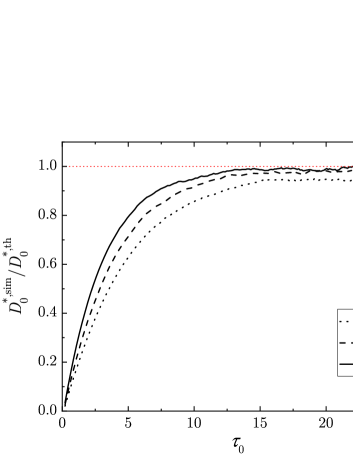
Figure 1: Dependence of the ratio $D_{0}^{\text{*,sim}}/D_{0}^{\text{*,th}}$ on the (dimensionless) time $\tau_{0}$ for a ternary mixture with $x_{1}=0.5$, $m_{0}/m_{1}=3$, $m_{0}/m_{2}=2$, $\sigma_{0}=\sigma_{1}=\sigma_{2}$, and three different values of the (common) coefficient of restitution $al_{ij}\equiv\alpha$: 0.9, 0.8, and 0.7. Here, $D_{0}^{\text{*,sim}}$ refers to the simulation result of the dimensionless tracer diffusion coefficient $D_{0}^{*}$ while $D_{0}^{\text{*,th}}$ corresponds to its theoretical result obtained from the first Sonine approximation.

According to Eq. (38), the validity of a hydrodynamic description implies necessarily that the time dependence of the diffusion coefficient $D_{0}(t)$ only occurs via the square root of the granular temperature $T(t)$ ($D_{0}(t)\propto\sqrt{T(t)}$ for hard spheres). Thus, the dimensionless diffusion coefficient $D_{0}^{*}$ must reach a constant value independent of time after a transient regime. Our simulation results clearly show that $D_{0}^{*}$ reaches a stationary value in all the systems simulated in the work. To illustrate this behaviour, we plot in Fig. 1 the ratio $D_{0}^{\text{*,sim}}/D_{0}^{\text{*,th}}$ versus the (dimensionless) time $\tau_{0}$, defined as the average number of collisions experienced by the tracer particles up to a time $t$. The relationship between $\tau_{0}(t)$ and $\tau(t)$ is given in the Appendix C. In Fig. 1, we consider a ternary mixture with $x_{1}=n_{1}/(n_{1}+n_{2})=0.5$, $m_{0}/m_{1}=3$, $m_{0}/m_{2}=2$, $\sigma_{0}=\sigma_{1}=\sigma_{2}$, and three different values of the (common) coefficient of restitution $\alpha_{ij}\equiv\alpha$: 0.9, 0.8, and 0.7. Moreover, $D_{0}^{\text{*,sim}}$ refers to the simulation result of the dimensionless tracer diffusion coefficient $D_{0}^{*}$ while $D_{0}^{\text{*,th}}$ corresponds to its theoretical result obtained from the first Sonine approximation. As occurs for binary systems (see Fig. 3 of Ref. Garzó and Montanero (2004)), we observe that after a certain number of collisions, $D_{0}^{\text{*,sim}}/D_{0}^{\text{*,th}}$ reaches a time-independent plateau, which value fluctuates around 1. This means that the value of the coefficient $D_{0}^{*}$ measured in the simulations agrees very well with the one obtained from the Boltzmann kinetic equation. Additionally, we can observe that the transition to the steady state takes more time the lower the value of $\alpha$. This is because, in these specific simulations, the initial values of the particle velocities are sampled from Maxwellian distributions at the same temperature. As the inelasticity increases, the breakdown of energy equipartition becomes more pronounced, and therefore, the longer it takes for the velocity distributions to relax to their stationary forms.

Table 1: Three-dimensional systems considered in the computer simulations

Case	$x_{1}$	$\frac{\sigma_{0}}{\sigma_{1}}$	$\frac{\sigma_{0}}{\sigma_{2}}$	$\frac{m_{0}}{m_{1}}$	$\frac{m_{0}}{m_{2}}$
I	0.5	1	1	3	2
II	0.8	1	1	$\frac{1}{2}$	$\frac{1}{4}$
III	$0.5$	$2^{1/3}$	$5^{1/3}$	2	5
IV	$0.9$	$\frac{10}{3}$	$\frac{1}{2}$	$(\frac{10}{3})^{3}$	$\frac{1}{8}$

Figure 2: Temperature ratios $T_{i}/T$ versus the (common) coefficient of restitution $\alpha$ for the cases I, II, III, and IV described in Table 1. The solid lines and circles correspond to $T_{0}/T$, the dashed lines and squares refer to $T_{1}/T$, while the dotted lines and triangles correspond to $T_{2}/T$. Symbols are the DSMC results while lines are the theoretical results.

Figure 3: Plot of the (reduced) tracer diffusion coefficient $D_{0}(\alpha)/D_{1}(1)$ as a function of the (common) coefficient of restitution $\alpha$ for the cases I, II, III, and IV described in Table 1. The solid and dashed lines refer to the theoretical results obtained from the second and first Sonine approximations, respectively, while the symbols (circles) refer to the DSMC results. Here, $D_{0}(1)$ denotes the elastic-limit value of the coefficient $D_{0}$ consistently obtained in each approximation.

Four different cases or systems have been considered in the simulations. In all of them we consider a common coefficient of restitution $\alpha_{ij}\equiv\alpha$. The values of concentration, masses, and diameters of the different systems are displayed in Table 1. In the two first cases (Cases I and II), we have considered a ternary system with identical diameters ($\sigma_{0}=\sigma_{1}=\sigma_{2}$) but different masses. In the cases III and IV, we have assumed that intruders and particles of the species 1 and 2 have the same mass density, namely, $m_{0}/m_{1}=(\sigma_{0}/\sigma_{1})^{3}$ and $m_{0}/m_{2}=(\sigma_{0}/\sigma_{2})^{3}$. Furthermore, since we are essentially interested in studying the influence of dissipation on the tracer diffusion coefficient, we have normalized $D_{0}(\alpha)$ with respect to its value for elastic collisions ($\alpha_{ij}=1$). Thus, the steady values of the ratio $D_{0}(\alpha)/D_{0}(1)$ obtained from simulation data are compared against their theoretical predictions obtained by considering the first [Eq. (57)] and second Sonine [Eq. (58)] approximations. The theoretical elastic value $D_{0}(1)$ has been consistently obtained in each approximation.

Before considering the diffusion coefficient, we study first the dependence of the temperature ratios $\gamma_{0}=T_{0}/T$, $\gamma_{1}=T_{1}/T$, and $\gamma_{2}=T_{2}/T$ on the coefficient of restitution. Note that in the tracer limit $\gamma_{2}=(1-x_{1}\gamma_{1})/(1-x_{1})$, so that only two of the temperature ratios are independent. Figure 2 shows the dependence of the temperature ratios on inelasticity for the cases considered in Table 1. The ratios $\gamma_{i}$ are obtained as described at the end of Sec. II.B. As expected, is it quite apparent that the total energy is not equally distributed between the different species. This means that there is a breakdown of energy equipartition in granular mixtures. As mentioned in Sec. II, the lack of energy equipartition in granular mixtures has been confirmed in many computer simulation works Montanero and Garzó (2002); Dahl et al. (2002); Barrat and Trizac (2002a, b); Clelland and Hrenya (2002); Krouskop and Talbot (2003); Wang et al. (2003); Brey et al. (2005, 2006); Schröter et al. (2006); Brey and Ruiz-Montero (2011); Bodrova et al. (2014); Vega Reyes et al. (2017); Bodrova et al. (2020) as well as in real experiments of agitated Wildman and Parker (2002); Feitosa and Menon (2002) and freely cooling Puzyrev et al. (2024) mixtures. In addition, the lack of energy equipartition has dramatic consequences in the case of a large impurity/gas mass ratio since there is a peculiar “phase transition” with one phase where the diffusion coefficient grows without bound Santos and Dufty (2001a, b).

As occurs for binary systems, it is quite apparent in Fig. 2 that for large differences in the mass ratios $m_{0}/m_{1}$ and $m_{0}/m_{2}$ the temperature ratios depart significantly from 1, even for relatively weak dissipation (say for instance, $\alpha\gtrsim 0.8$). We also observe that in general the temperature of the heavier species is larger than that of the lighter ones. Moreover, in spite that the temperature ratios $\gamma_{i}$ have been estimated by considering the simple Maxwellian approximations (24) to the scaled distributions $\varphi_{i}$, the theoretical predictions for $\gamma_{i}$ exhibit in general an excellent agreement with the DSMC results, even for strong inelasticities.

We consider now the (dimensionless) diffusion coefficient $D_{0}(\alpha)/D_{0}(1)$. Based on the previous results obtained for a binary system Garzó and Montanero (2004), one would expect that the first and second Sonine approximations practically coincide in the Rayleigh gas limit (namely, when the mass and/or the diameter of the intruder is larger than that of the granular gas particles) while both approximations appreciably differ in the Lorentz gas limit (namely, when the mass and/or the diameter of the intruder is smaller than that of the granular gas particles). Figure 3 shows the $\alpha$-dependence of $D_{0}(\alpha)/D_{0}(1)$ for the four cases displayed in Table 1. In case I, the mass of the intruder is larger than the mass of the particles of the granular gas mixture (a Rayleigh-like scenario). It is quite apparent from Fig. 3 that both Sonine approximations (Sonine of order 1 and Sonine of order 2) are close to each other in this case, although the second approximation is clearly better than the first one, especially when the collisional inelasticity is large (let’s say for instance, $\alpha\gtrsim 0.6$). Case II is the opposite of case I: now the intruder mass is smaller than that of the particles of the granular mixture (a Lorentz-like scenario). We observe that the two Sonine approximations differ significantly, especially for strong inelasticity. In addition, we see that while the first Sonine approximation clearly overestimates the computer simulation data, the agreement of the second Sonine approximation with the results of the DSMC is excellent in the complete range of values of $\alpha$ analyzed. In case III, the mass density of all particles (intruder and gas grains) is the same, but the particles of the granular mixture are larger and heavier than the intruder. This case is thus closer to the Rayleigh limit, and again we find that the two Sonine approximations give quite similar results. Finally, in case IV, the mass density of all particles is again the same, but now the grains of species 1 are larger and heavier than the intruder, while the grains of species 2 are smaller and lighter than the intruder. However, since most of the grains are of species 1 (since $x_{1}=0.9$), the scenario is more Rayleigh-like than Lorenz-like. As expected, we find that the two Sonine approximations give similar results, although again the second Sonine solution is the best, providing again a very good agreement with the DSMC results.

In summary, our results for the diffusion of intruders in a binary granular mixture (ternary system) share similarities with those previously reported Garzó and Montanero (2004) for a binary system: The second Sonine approximation clearly improves on the first Sonine approximation, especially when the intruders are lighter than the particles of the surrounding granular binary mixture. In the latter case, the first Sonine solution for $D_{0}$ clearly overestimates the simulation data, while the second Sonine approximation agrees very well with the DSMC results even for large values of the inelasticity.

VI Concluding remarks

The determination of the MSD of an intruder in a freely cooling granular mixture is a very interesting and not completely understood problem. There are likely two different reasons for which the problem is quite complex. First, there is a large number of relevant parameters involved in the description of diffusion in granular mixtures. Second, there is also a wide array of complexities that arise during the derivation of kinetic theory models. Thus, to gain some insight into the general problem, the first studies consider two limiting cases: (i) when the intruder is mechanically equivalent to the particles of the granular gas (self-diffusion problem) Brey et al. (2000); Brilliantov and Pöschel (2000); Bodrova et al. (2015a), and (ii) when the intruder is much more heavier than the particles of the granular gas (Brownian limiting case) Brey et al. (1999); Sarracino et al. (2010). One of the main conclusions in these studies is that the MSD of an intruder presents a logarithmic time dependence. According to Haff’s law Haff (1983), the origin of this logarithmic dependence arises from the algebraic decay of the granular temperature. These studies have been extended more recently to arbitrary values of the intruder-grain mass and/or diameter ratios Alam et al. (2019) and even when the system is immersed in a molecular gas (granular suspension) Gómez González et al. (2023).

Very recently Bodrova (2024), Bodrova has extended all the previous attempts to the case of granular mixtures with an arbitrary number of mechanically different species. On the other hand, to determine the expression of the MSD of the species $k$, one needs to know the diffusion coefficient $D_{k}(t)$. This coefficient is given in terms of the unknown $\boldsymbol{\mathcal{A}}_{k}(\mathbf{v})$ which is in fact the solution of the linear integral equation (50). Thus, as occurs for molecular hard spheres mixtures Chapman and Cowling (1970), the above integral equation cannot be exactly solved (except for the so-called inelastic Maxwell models Ben-Naim and Krapivsky (2003)) and hence, one has to expand $\boldsymbol{\mathcal{A}}_{k}(\mathbf{v})$ in a Sonine polynomial expansion. In Ref. Bodrova (2024), although not explicitly stated in the paper, the simplest first Sonine approximation (a first order polynomial in the particle velocity $\mathbf{v}$) to $\boldsymbol{\mathcal{A}}_{k}(\mathbf{v})$ is only considered. Although this approach can be accurate in some cases (for binary systems, when the intruder is much heavier than the particles of the granular gas), it yields a significant disagreement with computer simulations when the intruder is much lighter than the granular gas particles. In contrast, as has been widely shown in several papers for binary systems Garzó and Montanero (2004); Garzó and Vega Reyes (2009, 2012); Garzó et al. (2013); Gómez González and Garzó (2023, 2024), the second Sonine approximation to the diffusion coefficient improves the predictions of the first Sonine approximation since it leads in most of the cases to an excellent agreement with computer simulations. The determination of the tracer diffusion coefficient in a multicomponent granular mixture from the first and second Sonine approximations has been one of the main goals of the present contribution.

To assess the reliability of the Sonine approximations, we have also numerically solved the Boltzmann equation by means of the DSMC method Bird (1994) conveniently adapted to dissipative dynamics. Our simulations have been focused on the case of a ternary mixture where one of the species is present in tracer concentration. Four different sort of systems (displayed in Table 1) have been considered. As happens for binary systems Garzó and Montanero (2004), the comparison between theory and computer simulations clearly shows the superiority of the second Sonine solution over the first one, especially in case II (mass of intruders smaller than that of the particles of the granular gas) for strong inelasticity. In addition, the excellent agreement found between the second Sonine approximation to $D_{0}$ and DSMC results (see Fig. 3) confirms the accuracy of this theoretical expression for conditions of practical interest in mixtures constituted by three species. We expect that this good agreement will be kept in mixtures containing more than three species.

We want also to remark that the derivation carried out here for the MSD is slightly different to the one provided in Ref. Bodrova (2024). While in the above work Bodrova (2024) the MSD is obtained from the velocity correlation function, here we identify the MSD of an intruder immersed in a granular mixture through the diffusion equation. In any case, when the intruder is mechanically equivalent to one of the species (let’s say species $k$), then the MSD of the species $k$ derived here agrees with the one obtained in Ref. Bodrova (2024) when the first Sonine approximation to $D_{k}$ is considered.

One of the main limitations of the present work is its restriction to smooth inelastic hard spheres. This means that inelaticity in collisions only affects to the translational degrees of freedom. The extension of the results derived here to the case of inelastic rough hard spheres is an interesting open problem. Although some attempts have been made in the self-diffusion problem Bodrova and Brilliantov (2012), it still remains to assess the impact of particles’ roughness on diffusion when the intruder and particles of the granular gas are mechanically different. Another possible project may be the extension of the present results to granular suspensions where the influence of the interstitial fluid on grains can be modeled via a drag force plus a stochastic-like Langevin term Gómez González et al. (2023); Bao and Wang (2024). Work along these lines is in progress.

Appendix A First and second Sonine approximations to the diffusion coefficient $D_{0}$

In this appendix we give some technical details on the determination of the Sonine coefficients $a_{1}$ and $a_{2}$. Substitution of Eq. (52) into the integral equation (50) yields

$$\zeta T\partial_{T}\Big{(}a_{1}f_{0\text{M}}\mathbf{v}+a_{2}f_{0\text{M}}\mathbf{S}_{0}\Big{)}+a_{1}\sum_{i=1}^{s}J_{0i}[f_{0\text{M}}\mathbf{v},f_{i}]+a_{2}\sum_{i=1}^{s}J_{0i}[f_{0\text{M}}\mathbf{S}_{0},f_{i}]=-\frac{f_{0}^{(0)}}{n_{0}}\mathbf{v}.$$ (66)

Next, we multiply Eq. (66) by $\mathbf{v}$ and integrate over the velocity. The result is

$$\left(\nu_{a,0}-\frac{1}{2}\zeta\right)D_{0}+\frac{n_{0}T_{0}^{2}}{m_{0}}\nu_{b,0}\,a_{2}=\frac{T_{0}}{m_{0}},$$ (67)

where use has been made of the identity $a_{1}=(m_{0}D/n_{0}T_{0})$ and we have taken into account that $a_{1}T\propto T^{1/2}$ and so $T\partial_{T}a_{1}T=(1/2)a_{1}T$. Moreover, we have introduced the quantities

$$\nu_{a,0}=\sum_{i=1}^{s}\nu_{a,0i},\quad\nu_{a,0i}=-\frac{m_{0}}{dn_{0}T_{0}}\int d\mathbf{v}\;\mathbf{v}\cdot J_{0i}[f_{0\text{M}}\mathbf{v},f_{i}],$$ (68)

$$\nu_{b,0}=\sum_{i=1}^{s}\nu_{b,0i},\quad\nu_{b,0i}=-\frac{m_{0}}{dn_{0}T_{0}^{2}}\int d\mathbf{v}\;\mathbf{v}\cdot J_{0}[f_{0\text{M}}\mathbf{S}_{0},f_{i}].$$ (69)

If only the first Sonine correction is retained ($a_{2}=0$), the solution to Eq. (67) is simply

$$D_{0}[1]=\frac{T_{0}/m_{0}}{\nu_{a,0}-\frac{1}{2}\zeta}.$$ (70)

Equation (70) leads to Eq. (57).

To close the problem, one has to multiply Eq. (67) by $\mathbf{S}_{0}(\mathbf{v})$ and integrate over $\mathbf{v}$. After some algebra, one achieves the result

$$\Big{(}\nu_{c,0}-\zeta\Big{)}\frac{m_{0}D_{0}}{n_{0}T_{0}^{2}}+\left(\nu_{d,0}-\frac{3}{2}\zeta\right)a_{2}=0,$$ (71)

where

$$\nu_{c,0}=\sum_{i=1}^{s}\nu_{c,0i},\quad\nu_{d,0}=\sum_{i=1}^{s}\nu_{d,0i}.$$ (72)

Here,

$$\nu_{c,0i}=-\frac{2}{d(d+2)}\frac{m_{0}}{n_{0}T_{0}^{2}}\int d\mathbf{v}\;\mathbf{S}_{0}\cdot J_{0i}[f_{0\text{M}}\mathbf{v},f_{i}],$$ (73)

$$\nu_{d,0i}=-\frac{2}{d(d+2)}\frac{m_{0}}{n_{0}T_{0}^{3}}\int d\mathbf{v}\;\mathbf{S}_{0}\cdot J_{0i}[f_{0\text{M}}\mathbf{S}_{0},f_{i}].$$ (74)

In reduced units and using matrix notation, Eqs. (67) and (71) can be rewritten as

$$\left(\begin{array}[]{cc}\nu_{a,0}^{*}-\frac{1}{2}\zeta^{*}&\gamma_{0}^{2}\nu_{b,0}^{*}\\ \frac{\nu_{c,0}^{*}-\zeta^{*}}{\gamma_{0}^{2}}&\nu_{d,0}^{*}-\frac{1}{2}\zeta^{*}\end{array}\right)\left(\begin{array}[]{c}D_{0}^{*}\\ a_{2}^{*}\end{array}\right)=\left(\begin{array}[]{c}\gamma_{0}\\ 0\end{array}\right).$$ (75)

Here, $D_{0}^{*}=(m_{0}\nu/T)D_{0}$, $a_{2}^{*}=n_{0}T\nu a_{2}$, $\nu_{a,0}^{*}=\nu_{a,0}/\nu$, $\nu_{b,0}^{*}=\nu_{b,0}/\nu$, $\nu_{c,0}^{*}=\nu_{c,0}/\nu$, and $\nu_{d,0}^{*}=\nu_{d,0}/\nu$. The solution to Eq. (75) gives the expression (58) of the second Sonine approximation $D_{0}^{*}[2]$ to $D_{0}^{*}$.

Appendix B Reduced collision frequencies

To obtain the explicit dependence of $D_{0}^{*}[2]$ and $D_{0}^{*}[1]$ on the parameter space of the system, one still needs to determine the quantities $\nu_{a,0}^{*}$, $\nu_{b,0}^{*}$, $\nu_{c,0}^{*}$, and $\nu_{d,0}^{*}$. According to Eqs. (68), (69), (72), (73), and (74), the above reduced collision frequencies are given in terms of the quantities $\nu_{a,0i}^{*}$, $\nu_{b,0i}^{*}$, $\nu_{c,0i}^{*}$, and $\nu_{d,0i}^{*}$. These quantities have been evaluated in previous works when the distribution $f_{i}$ is approximated by the Maxwellian distribution given by Eq. (85).

To display the final expressions, it is convenient to introduce the quantities

$$\theta_{0}=\frac{m_{0}T}{\overline{m}T_{0}},\quad\lambda_{0i}=\mu_{0i}\theta_{i}-\mu_{i0}\theta_{0},$$ (76)

and $\theta_{i}$ defined in Eq. (24). In terms of these quantities, $\nu_{a,0i}^{*}$, $\nu_{b,0i}^{*}$, $\nu_{c,0i}^{*}$, and $\nu_{d,0i}^{*}$ are given, respectively, by

$$\nu_{a,0i}^{*}=\frac{2\pi^{(d-1)/2}}{d\Gamma\left(\frac{d}{2}\right)}x_{i}\left(\frac{\sigma_{0i}}{\overline{\sigma}}\right)^{d-1}\chi_{0i}\mu_{i0}(1+\alpha_{0i})\left(\frac{\theta_{0}+\theta_{i}}{\theta_{i}\theta_{0}}\right)^{1/2},$$ (77)

$$\nu_{b,0i}^{*}=\frac{\pi^{(d-1)/2}}{d\Gamma\left(\frac{d}{2}\right)}x_{i}\left(\frac{\sigma_{0i}}{\overline{\sigma}}\right)^{d-1}\chi_{0i}\mu_{i0}(1+\alpha_{0i})\left[\frac{\theta_{i}}{\theta_{0}(\theta_{i}+\theta_{0})}\right]^{1/2},$$ (78)

$$\nu_{c,0i}^{*}=\frac{2\pi^{(d-1)/2}}{d(d+2)\Gamma\left(\frac{d}{2}\right)}x_{i}\left(\frac{\sigma_{0i}}{\overline{\sigma}}\right)^{d-1}\chi_{0i}\mu_{i0}(1+\alpha_{0i})\left(\theta_{i}+\theta_{0}\right)^{-1/2}\theta_{i}^{-3/2}\theta_{0}^{1/2}A_{c},$$ (79)

$$\nu_{d,0i}^{*}=\frac{\pi^{(d-1)/2}}{d(d+2)\Gamma\left(\frac{d}{2}\right)}x_{i}\left(\frac{\sigma_{0i}}{\overline{\sigma}}\right)^{d-1}\chi_{0i}\mu_{i0}(1+\alpha_{0i})\left(\frac{\theta_{0}}{\theta_{i}(\theta_{0}+\theta_{i})}\right)^{3/2}\left[A_{d}-(d+2)\frac{\theta_{i}+\theta_{0}}{\theta_{0}}A_{c}\right],$$ (80)

where

$$A_{c} = (d+2)(2\lambda_{0i}+\theta_{i})+\mu_{i0}(\theta_{0}+\theta_{i})\left\{(d+2)(1-\alpha_{0i})-[(11+d)\alpha_{0i}-5d-7]\lambda_{0i}\theta_{0}^{-1}\right\}$$ (81)

$$+3(d+3)\lambda_{0i}^{2}\theta_{0}^{-1}+2\mu_{i0}^{2}\left(2\alpha_{0i}^{2}-\frac{d+3}{2}\alpha_{0i}+d+1\right)\theta_{0}^{-1}(\theta_{0}+\theta_{i})^{2}-(d+2)\theta_{i}\theta_{0}^{-1}(\theta_{0}+\theta_{i}),$$

$$A_{d} = 2\mu_{i0}^{2}\theta_{0}^{-2}(\theta_{0}+\theta_{i})^{2}\left(2\alpha_{0i}^{2}-\frac{d+3}{2}\alpha_{0i}+d+1\right)\left[(d+2)\theta_{0}+(d+5)\theta_{i}\right]$$ (82)

$$-\mu_{i0}(\theta_{0}+\theta_{i})\Big{[}\lambda_{0i}\theta_{0}^{-2}\big{\{}(d+2)\theta_{0}+(d+5)\theta_{i}\big{\}}\big{\{}(11+d)\alpha_{0i}-5d-7\big{\}}$$

$$-\theta_{i}\theta_{0}^{-1}\big{\{}20+d(15-7\alpha_{0i})+d^{2}(1-\alpha_{0i})-28\alpha_{0i}\big{\}}-(d+2)^{2}(1-\alpha_{0i})\Big{]}$$

$$+3(d+3)\lambda_{0i}^{2}\theta_{0}^{-2}[(d+2)\theta_{0}+(d+5)\theta_{i}]+2\lambda_{0i}\theta_{0}^{-1}[(d+2)^{2}\theta_{0}+(24+11d+d^{2})\theta_{i}]$$

$$+(d+2)\theta_{i}\theta_{0}^{-1}[(d+8)\theta_{0}+(d+3)\theta_{i}]-(d+2)(\theta_{0}+\theta_{i})\theta_{0}^{-2}\theta_{i}[(d+2)\theta_{0}+(d+3)\theta_{i}].$$

Appendix C Collision frequency of the intruders

In this appendix, we provide the relationship between the dimensionless times $\tau_{0}(t)$ (defined as the average number of collisions suffered by the intruders up to a time $t$) and $\tau(t)$ [defined by Eq. (39)]. To establish this relation one has to evaluate the (average) collision frequency of the intruders $\nu_{0}(t)$. For hard spheres, $\nu_{0}(t)$ is defined as

$$\nu_{0}(t)=\sum_{i=1}^{s}\nu_{0i}(t),$$ (83)

where

$$\nu_{0i}(t) = n_{0}^{-1}\sigma_{0i}^{d-1}\chi_{0i}\int d\mathbf{v}_{1}\int d\mathbf{v}_{2}\int d\widehat{\boldsymbol{\sigma}}\,\Theta(\widehat{{\boldsymbol{\sigma}}}\cdot{\bf g}_{12})$$ (84)

$$\times(\widehat{\boldsymbol{\sigma}}\cdot{\bf g}_{12})f_{i}(\mathbf{v}_{1};t)f_{0}(\mathbf{v}_{2};t),$$

where $f_{i}(\mathbf{v}_{1};t)$ and $f_{0}(\mathbf{v}_{2};t)$ are the velocity distribution functions of the particles of the species $i$ and the intruders, respectively. The integrals appearing in Eq. (84) are evaluated here by considering the Maxwellian approximations to $f_{i}$ and $f_{0}$, namely,

$$f_{i}(\mathbf{v}_{1})\to n_{i}\pi^{-d/2}v_{\text{th}}^{-d}\theta_{i}^{d/2}e^{-\theta_{i}c_{1}^{2}},$$ (85)

$$f_{0}(\mathbf{v}_{2})\to n_{0}\pi^{-d/2}\theta_{0}^{d/2}v_{\text{th}}^{-d}e^{-\theta_{0}c_{2}^{2}},$$ (86)

where $\mathbf{c}_{i}=\mathbf{v}_{i}/v_{\text{th}}$. We recall that $v_{\text{th}}=\sqrt{2T/\overline{m}}$, $\theta_{i}=m_{i}T/(\overline{m}T_{i})$, and $\theta_{0}=m_{0}T/(\overline{m}T_{0})$. Thus, $\nu_{0i}$ can be rewritten as

$$\nu_{0i}(t)=n_{i}\sigma_{0i}^{d-1}\chi_{0i}(\theta_{i}\theta_{0})^{d/2}v_{\text{th}}(t)I_{\nu},$$ (87)

where we have introduced the dimensionless integral

$$I_{\nu}=\pi^{-d}\int d\mathbf{c}_{1}\int d\mathbf{c}_{2}\int d\widehat{\boldsymbol{\sigma}}\,\Theta(\widehat{{\boldsymbol{\sigma}}}\cdot{\bf g}_{12}^{*})(\widehat{\boldsymbol{\sigma}}\cdot{\bf g}_{12}^{*})e^{-\theta_{i}c_{1}^{2}-\theta_{0}c_{2}^{2}}.$$ (88)

Here, $\mathbf{g}_{12}^{*}=\mathbf{g}_{12}/v_{\text{th}}$. The integral $I_{\nu}$ can be performed by the change of variables $\mathbf{x}=\mathbf{c}_{1}-\mathbf{c}_{2}$, $\mathbf{y}=\theta_{i}\mathbf{c}_{1}+\theta_{0}\mathbf{c}_{2}$, with the Jacobian $(\theta_{i}+\theta_{0})^{-d}$. The integral $I_{\nu}$ gives

$$I_{\nu} = \pi^{-d}\frac{S_{d}^{2}}{\pi^{(d+1)/2}\,\Gamma\left(\frac{d+1}{2}\right)}\,(\theta_{i}+\theta_{0})^{-d}\int_{0}^{\infty}dx\,x^{d}e^{-ax^{2}}$$ (89)

$$\times\int_{0}^{\infty}dy\,y^{d-1}e^{-by^{2}},$$

where $S_{d}=2\pi^{d/2}/\Gamma(d/2)$ is the total solid angle in $d$ dimensions, $a\equiv\theta_{i}\theta_{0}(\theta_{i}+\theta_{0})^{-1}$, $b\equiv(\theta_{i}+\theta_{0})^{-1}$ and use has been made of the result van Noije and Ernst (1998)

$$\int d\widehat{\boldsymbol{\sigma}}\,\Theta(\widehat{{\boldsymbol{\sigma}}}\cdot{\bf g}_{12}^{*})(\widehat{\boldsymbol{\sigma}}\cdot{\bf g}_{12}^{*})=\frac{\pi^{(d-1)/2}}{\Gamma\left(\frac{d+1}{2}\right)}\,\mbox{g}_{12}^{*}.$$ (90)

The integral $I_{\nu}$ gives

$$I_{\nu}=\frac{\pi^{(d-1)/2}}{\Gamma\left(\frac{d}{2}\right)}(\theta_{i}\theta_{0})^{-\frac{d+1}{2}}\left(\theta_{i}+\theta_{0}\right)^{1/2},$$ (91)

and hence, $\nu_{0i}$ can be finally written as

$$\nu_{0i}(t) = \frac{\pi^{(d-1)/2}}{\Gamma\left(\frac{d}{2}\right)}n_{i}\sigma_{0i}^{d-1}\chi_{0i}\left(\frac{\theta_{i}+\theta_{0}}{\theta_{i}\theta_{0}}\right)^{1/2}v_{\text{th}}(t)$$

$$= \frac{\pi^{(d-1)/2}}{\Gamma\left(\frac{d}{2}\right)}x_{i}\left(\frac{\sigma_{0i}}{\overline{\sigma}}\right)^{d-1}\chi_{0i}\left(\frac{\theta_{i}+\theta_{0}}{\theta_{i}\theta_{0}}\right)^{1/2}\nu(t).$$

The (dimensionless) time $\tau_{0}(t)$ is defined as

$$\tau_{0}(t)=\int_{0}^{t}dt^{\prime}\nu_{0}(t^{\prime})=\sum_{i=1}^{s}\int_{0}^{t}dt^{\prime}\nu_{0i}(t^{\prime}).$$ (93)

Thus, according to Eq. (C), the relationship between $\tau_{0}(t)$ and $\tau(t)$ is

$$\tau_{0}(t)=\int_{0}^{t}dt^{\prime}\,\tau(t^{\prime})\,\sum_{i=1}^{s}A_{0i}(t^{\prime}),$$ (94)

where

$$A_{0i}\equiv\frac{\pi^{(d-1)/2}}{\Gamma\left(\frac{d}{2}\right)}x_{i}\left(\frac{\sigma_{0i}}{\overline{\sigma}}\right)^{d-1}\chi_{0i}\left(\frac{\theta_{i}+\theta_{0}}{\theta_{i}\theta_{0}}\right)^{1/2}.$$ (95)

References

- Ottino and Khakhar (2000) J. M. Ottino and D. V. Khakhar, “Mixing and segregation of granular fluids,” Ann. Rev. Fluid Mech. 32, 55–91 (2000).
- Kudrolli (2004) A. Kudrolli, “Size separation in vibrated granular matter,” Rep. Prog. Phys. 67, 209–247 (2004).
- Goldhirsch (2003) I. Goldhirsch, “Rapid granular flows,” Annu. Rev. Fluid Mech. 35, 267–293 (2003).
- Brilliantov and Pöschel (2004) N. Brilliantov and T. Pöschel, Kinetic Theory of Granular Gases (Oxford University Press, Oxford, 2004).
- Garzó (2019) V. Garzó, Granular Gaseous Flows (Springer Nature, Cham, 2019).
- Ippolito et al. (1995) I. Ippolito, C. Annic, J. Lemaître, L. Oger, and D. Bideau, “Granular temperature: experimental analysis,” Phys. Rev. E 52, 2072–2075 (1995).
- S. and Urbach (1999) Olafsen J. S. and J. S. Urbach, “Velocity distributions and density fluctuations in a granular gas,” Phys. Rev. E 60, 2468–2471 (1999).
- Wildman et al. (2001) R. D. Wildman, J. M. Huntley, and D. J. Parker, “Granular temperature profiles in three-dimensional vibrofluidized granular beds,” Phys. Rev. E 63, 061311 (2001).
- Melby et al. (2005) P. Melby, F. Vega Reyes, A. Prevost, R. Robertson, P. Kumar, D.A. Egolf, and J. S. Urbach, “The dynamics of thin vibrated granular layers,” J. Phys.: Condens. Matter 17, S2689–S2704 (2005).
- Gómez González et al. (2023) R. Gómez González, E. Abad, S. B. Yuste, and V. Garzó, “Diffusion of intruders in granular suspensions: Enskog theory and random walk interpretation,” Phys. Rev. E 108, 024903 (2023).
- Brey et al. (2000) J. J. Brey, M. J. Ruiz-Montero, D. Cubero, and R. García-Rojo, “Self-diffusion in freely evolving granular gases,” Phys. Fluids. 12, 876–883 (2000).
- Brilliantov and Pöschel (2000) N. V. Brilliantov and T. Pöschel, “Velocity distribution in granular gases of viscoelastic particles,” Phys. Rev. E 61, 5573–5587 (2000).
- Bodrova et al. (2015a) A. S. Bodrova, A. V. Chechkin, A. G. Cherstvy, and R. Metzler, “Quantifying non-ergodics dynamics of force-free granular gases,” Phys. Chem. Chem. Phys. 17, 21791–21798 (2015a).
- Brey et al. (1999) J. J. Brey, M. J. Ruiz-Montero, R. García-Rojo, and J. W. Dufty, “Brownian motion in a granular gas,” Phys. Rev. E 60, 7174–7181 (1999).
- Sarracino et al. (2010) A. Sarracino, D. Villamaina, G. Costantini, and A. Puglisi, “Granular Brownian motion,” J. Stat. Mech. P04013 (2010).
- Haff (1983) P. K. Haff, “Grain flow as a fluid-mechanical phenomenon,” J. Fluid Mech. 134, 401–430 (1983).
- Abad et al. (2022) E. Abad, S. B. Yuste, and V. Garzó, “On the mean square displacement of intruders in freely cooling granular gases,” Granular Matter 24, 111 (2022).
- Bodrova (2024) A. S. Bodrova, “Diffusion in multicomponent granular mixtures,” Phys. Rev. E 109, 024903 (2024).
- Garzó and Montanero (2004) V. Garzó and J. M. Montanero, “Diffusion of impurities in a granular gas,” Phys. Rev. E 69, 021301 (2004).
- Garzó and Vega Reyes (2009) V. Garzó and F. Vega Reyes, “Mass transport of impurities in a moderately dense granular gas,” Phys. Rev. E 79, 041303 (2009).
- Garzó and Vega Reyes (2012) V. Garzó and F. Vega Reyes, “Segregation of an intruder in a heated granular gas,” Phys. Rev. E 85, 021308 (2012).
- Garzó et al. (2013) V. Garzó, J. A. Murray, and F. Vega Reyes, “Diffusion transport coefficients for granular binary mixtures at low density: Thermal diffusion segregation,” Phys. Fluids 25, 043302 (2013).
- Gómez González and Garzó (2023) R. Gómez González and V. Garzó, “Tracer diffusion coefficients in a moderately dense granular suspension: Stability analysis and thermal diffusion segregation,” Phys. Fluids 35, 083318 (2023).
- Gómez González and Garzó (2024) R. Gómez González and V. Garzó, “Mobility and diffusion of intruders in granular suspensions. Einstein relation,” J. Stat. Mech. 023211 (2024).
- Bird (1994) G. A. Bird, Molecular Gas Dynamics and the Direct Simulation Monte Carlo of Gas Flows (Clarendon, Oxford, 1994).
- Garzó and Dufty (1999) V. Garzó and J. W. Dufty, “Homogeneous cooling state for a granular mixture,” Phys. Rev. E 60, 5706–5713 (1999).
- Montanero and Garzó (2002) J. M. Montanero and V. Garzó, “Monte Carlo simulation of the homogeneous cooling state for a granular mixture,” Granular Matter 4, 17–24 (2002).
- Barrat and Trizac (2002a) A. Barrat and E. Trizac, “Lack of energy equipartition in homogeneous heated binary granular mixtures,” Granular Matter 4, 57–63 (2002a).
- Dahl et al. (2002) S. R. Dahl, C. M. Hrenya, V. Garzó, and J. W. Dufty, “Kinetic temperatures for a granular mixture,” Phys. Rev. E 66, 041301 (2002).
- Brey et al. (2005) J. J. Brey, M. J. Ruiz-Montero, and F. Moreno, “Energy partition and segregation for an intruder in a vibrated granular system under gravity,” Phys. Rev. Lett. 95, 098001 (2005).
- García Chamorro et al. (2022) M. García Chamorro, R. Gómez González, and V. Garzó, “Kinetic theory of polydisperse granular mixtures: Influence of the partial temperatures on transport properties-A review,” Entropy 24, 826 (2022).
- van Noije and Ernst (1998) T. P. C. van Noije and M. H. Ernst, “Velocity distributions in homogeneous granular fluids: the free and heated case,” Granular Matter 1, 57–64 (1998).
- Garzó et al. (2007) V. Garzó, C. M. Hrenya, and J. W. Dufty, “Enskog theory for polydisperse granular mixtures. II. Sonine polynomial approximation,” Phys. Rev. E 76, 031304 (2007).
- Pagnani et al. (2002) R. Pagnani, U. M. B. Marconi, and A. Puglisi, “Driven low density granular mixtures,” Phys. Rev. E 66, 051304 (2002).
- Barrat and Trizac (2002b) A. Barrat and E. Trizac, “Molecular dynamics simulations of vibrated granular gases,” Phys. Rev. E 66, 051303 (2002b).
- Clelland and Hrenya (2002) R. Clelland and C. M. Hrenya, “Simulations of a binary-sized mixture of inelastic grains in rapid shear flow,” Phys. Rev. E 65, 031301 (2002).
- Krouskop and Talbot (2003) P. Krouskop and J. Talbot, “Mass and size effects in three-dimensional vibrofluidized granular mixtures,” Phys. Rev. E 68, 021304 (2003).
- Wang et al. (2003) H. Wang, G. Jin, and Y. Ma, “Simulation study on kinetic temperatures of vibrated binary granular mixtures,” Phys. Rev. E 68, 031301 (2003).
- Schröter et al. (2006) M. Schröter, S. Ulrich, J. Kreft, J. B. Swift, and H. L. Swinney, “Mechanisms in the size segregation of a binary granular mixture,” Phys. Rev. E 74, 011307 (2006).
- Wildman and Parker (2002) R. D. Wildman and D. J. Parker, “Coexistence of two granular temperatures in binary vibrofluidized beds,” Phys. Rev. Lett. 88, 064301 (2002).
- Feitosa and Menon (2002) K. Feitosa and N. Menon, “Breakdown of energy equipartition in a 2D binary vibrated granular gas,” Phys. Rev. Lett. 88, 198301 (2002).
- Puzyrev et al. (2024) D. Puzyrev, T. Trittel, K. Harth, and Stannarius, “Cooling of a granular gas mixture in microgravity,” npj Microgravity 10, 36 (2024).
- Chapman and Cowling (1970) S. Chapman and T. G. Cowling, The Mathematical Theory of Nonuniform Gases (Cambridge University Press, Cambridge, 1970).
- Bodrova et al. (2015b) A. S. Bodrova, A. V. Chechkin, A. G. Cherstvy, and R. Metzler, “Ultraslow scaled Brownian motion,” New J. Phys. 17, 063038 (2015b).
- Note (1) Note that the evaluation of the scaling time involves quantities associated with all the species of the multicomponent mixture since . However, in Ref. Bodrova (2024), the quantity is defined in Eq. (28), which is restricted to a monocomponent granular gas.
- Brey et al. (2006) J. J. Brey, M. J. Ruiz-Montero, and F. Moreno, “Hydrodynamic profiles for an impurity in an open vibrated granular gas,” Phys. Rev. E 73, 031301 (2006).
- Brey and Ruiz-Montero (2011) J. J. Brey and M. J. Ruiz-Montero, “Cooling rates and energy partition in inhomogeneous fludized granular mixtures,” Phys. Rev. E 84, 031302 (2011).
- Bodrova et al. (2014) A. S. Bodrova, D. Levchenko, and N. V. Brilliantov, “Universality of temperature distribution in granular gas mixtures with a steep particle size distribution,” Europhys. Lett. 106, 14001 (2014).
- Vega Reyes et al. (2017) F. Vega Reyes, A. Lasanta, A. Santos, and V. Garzó, “Energy nonequipartition in gas mixtures of inelastic rough hard spheres: The tracer limit,” Phys. Rev. E 96, 052901 (2017).
- Bodrova et al. (2020) A. S. Bodrova, A. Osinsky, and N. V. Brilliantov, “Temperature distribution in driven granular mixtures does not depend on mechanism on energy dissipation,” Sci. Rep. 10, 693 (2020).
- Santos and Dufty (2001a) A. Santos and J. W. Dufty, “Critical behavior of a heavy particle in a granular fluid,” Phys. Rev. Lett. 86, 4823–4826 (2001a).
- Santos and Dufty (2001b) A. Santos and J. W. Dufty, “Nonequilibrium phase transition for a heavy particle in a granular fluid,” Phys. Rev. E 64, 051305 (2001b).
- Alam et al. (2019) M. Alam, S. Saha, and R. Gupta, “Unified theory for a sheared gas-solid suspension: from rapid granular suspension to its small-Stokes-number limit,” J. Fluid Mech. 870, 1175–1193 (2019).
- Ben-Naim and Krapivsky (2003) E. Ben-Naim and P. L Krapivsky, “The Inelastic Maxwell Model,” in Granular Gas Dynamics, Lectures Notes in Physics, Vol. 624, edited by T. Pöschel and S. Luding (Springer, 2003) pp. 65–94.
- Bodrova and Brilliantov (2012) A. S. Bodrova and N. Brilliantov, “Self-diffusion in granular gases: an impact of particles’ roughness,” Granular Matter 14, 85 (2012).
- Bao and Wang (2024) Jing-Dong Bao and Xiang-Rong Wang, “Generalized Einstein relation for aging processes,” Communications Physics 7, 294 (2024).