Efficient FPGA Implementation of an Optimized SNN-based DFE for Optical Communications

Abstract

The ever-increasing demand for higher data rates in communication systems intensifies the need for advanced non-linear equalizers capable of higher performance. Recently artificial neural networks were introduced as a viable candidate for advanced non-linear equalizers, as they outperform traditional methods. However, they are computationally complex and therefore power hungry. snn started to gain attention as an energy-efficient alternative to ANNs. Recent works proved that they can outperform ANNs at this task. In this work, we explore the design space of an spiking neural network (SNN)-based decision-feedback equalizer (DFE) to reduce its computational complexity for an efficient implementation on field programmable gate array (FPGA). Our Results prove that it achieves higher communication performance than ANN-based DFE at roughly the same throughput and at $25\times$ higher energy efficiency.

I Introduction

Data rates of modern communication systems increased dramatically in recent years. This leads to severe degradations of the communication performance caused by noise, inter-symbol interference (ISI), and hardware impairments, increasing the demand for advanced equalizers capable of migrating non-linear distortions.

Latest research showed that ANNs are a promising candidate to solve the problem of channel equalization for next-gen communication systems [1, 2, 3, 4]. Since ANNs are able to compensate for non-linearities, they can achieve higher performance than equalizers based on traditional linear filters. Additionally, they are highly flexible and can be designed to adapt to channel variations by retraining [5, 6]. However, compared to traditional methods, ANNs are computationally complex, which makes efficient hardware implementation challenging. Especially on embedded devices, the practical application of ANNs is limited due to the high power consumption and energy requirements.

To solve the problem of stringent power and energy requirements of ANNs, researchers started investigating the use of SNNs, which are inspired by the human brain to provide high energy efficiency. Two characteristics help to achieve this goal. Firstly, neurons in an SNN communicate using binary spikes instead of high-precision activations commonly used in ANNs. Secondly, SNNs are event-based networks. Hence, neurons only process information if they receive an input. Recent works showed that SNNs can even outperform ANNs for the task of equalization of an optical communication channel [7, 8, 9].

A commonly used platform for the implementation of digital signal processing algorithms are FPGAs since they enable parallel processing, allow for arbitrary precision and are highly flexible. In contrast to neuromorphic hardware, often used for the implementation of SNNs, FPGAs are widely used in real-world communication systems and are therefore a feasible solution for the implementation of the SNN-based equalizer.

In this work, we take a first step towards the practical application of SNN-based equalization by providing an efficient FPGA implementation of the equalizer investigated on an algorithmic level in [7]. A detailed SNN design-space-exploration is performed and a novel hardware implementation is presented.

The new contributions of our work are:

• We perform a detailed design-space-exploration of the SNN topology and a trade-off analysis of complexity vs. communication performance.

• We present a custom, flexible FPGA architecture of the Leaky-Integrate-and-Fire (LIF) neuron, commonly used in SNNs.

• We evaluate the hardware performance of the SNN-based equalizer and compare it to its ANN counterpart regarding resource utilization, power consumption and energy efficiency.

• We show that SNN implementations can outperform ANN implementations in terms of energy efficiency even on synchronous, digital platforms like FPGAs while maintaining better communication performance. Thus, our SNN implementation outperforms state-of-the-art regarding communication performance and hardware energy efficiency.

• To the best of our knowledge this is the first FPGA implementation of an SNN-based DFE for optical communications.

II Channel Model

As transmission link we select the optical fiber channel with intensity-modulation direct detection (IM/DD) and pulse-amplitude modulation (PAM) proposed by [8] which is also used in [7]. As shown in Fig. 1 the transmitted symbols $\mathbf{x}$ are upsampled by a factor of two and convolved with a root-raised-cosine (RRC) pulse shaping filter with a roll-off factor of $0.2$ at the transmitter. The simulated optical fiber channel applies chromatic dispersion (CD) with a fiber dispersion coefficient of $17\text{\,}$ followed by square-law detection which distorts the signal nonlinearly. Afterwards, the signal is superimposed by additive white Gaussian noise (AWGN) with zero mean and unit variance. At receiver side, the signal is RRC-filtered and downsampled. Finally, the SNN-based equalizer is applied to compensate for the distortions of the channel by producing an estimate of the transmitted symbol, given as $\bm{\tilde{x}}$. In particular, the channel has the following parameters: a fiber length of $5\text{\,}$, a data rate of $50\text{\,}\mathrm{G}\mathrm{B}\mathrm{d}$, and a wavelength of $1550\text{\,}$. Further, PAM-4 is applied where the symbols $\mathcal{C}=\{0,1,\sqrt{2},\sqrt{3}\}$ are transmitted with Gray mapping. This configuration corresponds to the channel B introduced in [7].

Due to CD in combination with square-law detection, the transmitted signal is distorted nonlinearly. Those distortions can’t be compensated by conventional linear equalizers. This motivates for the use of either traditional DFEs or modern neural network (NN)-based equalization approach due to their ability to compensate for nonlinear impairments [10].

Figure 1: Model of the optical communication chain. Data is sent from a transmitter over an optical fiber channel with CD and square-law detection to a receiver including the SNN-based equalizer.

III Spiking Neural Networks

snn are the next generation of NNs[11]. The main difference between SNNs and ANNs is that their functionality is more similar to that of the human brain, in which neurons communicate by action potentials. On digital devices, action potentials can be modelled as binary signals. This simplifies the hardware implementation and increases the energy efficiency. Furthermore, biological neurons work in an event-based way; as a result, they perform calculations only if they receive an input spike. Consequently SNNs are expected to be more energy efficient than similarly sized ANNs.

SNNs are time-dependent, in other words, for each input sample the network runs for a specific number of iterations or time steps. The various neurons charge or discharge at each time step according to their internal parameters and the state of their input.

Multiple neuron models were developed to mimic the biological neurons. They range from accurate or biologically plausible such as the Hodgkin-Huxley[12] model to simple ones; that do not support most of the biological features but have lower computational complexity such as the LIF model.

III-A lif model

The LIF model is a commonly used neuron model. A recurrent version of the model is described by (1) and (2) [13]:

$$\frac{dv(t)}{dt}=-\frac{(v(t)-v_{r})+ri(t)}{\tau_{m}}+\Theta(v(t)-v{{}_{\mathrm{th}}})(v_{r}-v{{}_{\mathrm{th}}})$$ (1)

$$\frac{di(t)}{dt}=-\frac{i(t)}{\tau_{s}}+\sum_{j}w_{j}s_{j}(t)+\sum_{j}v_{j}s_{r}j(t)$$ (2)

Where $v(t)$ is the voltage or membrane potential, $v_{r}$ is the reset voltage, $r$ is the input resistance, $i(t)$ is the input current, $\Theta(\cdot)$ denotes the Heaviside function, $v{{}_{\mathrm{th}}}$ is the threshold voltage, $\tau_{m}$ is the voltage-time constant, $\tau_{s}$ is the input time constant, $w_{j}$ is the input weight, $s_{j}(t)$ is the input from the previous layer, $v_{j}$ is the weight of the recurrent connection and $s_{r}j(t)$ is the input from the recurrent connection. Fig. 2 illustrates the working principle of the LIF model. Once an input spike is received the voltage increases and then starts to decay; $\tau_{m}$ controls the decaying speed. The input current also decays with a factor of $\tau_{s}$. If multiple consecutive spikes are received by the neuron the voltage increases till it exceeds the threshold; then an output spike is generated and the voltage is set to the reset voltage.

Figure 2: Simulation of the LIF model. Voltage and current increase with the arrival of new spikes and an output spike is generated if the voltage reaches $v_{\mathrm{th}}$, after which it’s set to $v_{\mathrm{r}}$

III-B SNN structure

This work is based on the SNN-DFE network presented in [7], referred to later as the reference topology. The structure of the reference topology is illustrated in Fig. 3, it consists of three components: the linear input layer, the LIF recurrent block, and the linear output layer. The LIF recurrent block consists of three layers: a linear input layer, a recurrent linear layer, and an activation layer consisting of the LIF neurons. The topology processes the input in the following way using ten time steps. For the first time step the input is encoded using the encoding mechanism introduced in [9] and passed to the network. For the remaining nine steps zeros are passed as input. On the output side, the output of each neuron is accumulated over the time steps and the output with the highest value is considered as the final decision.

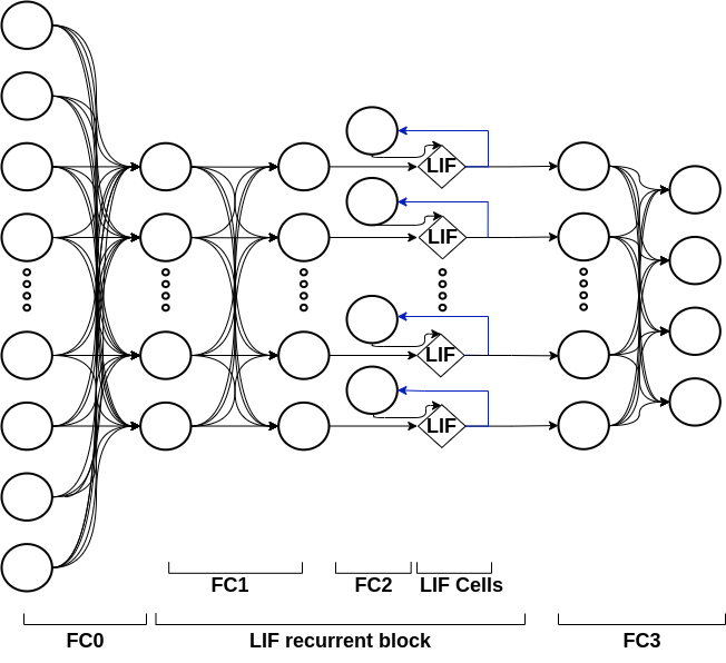
Figure 3: The architecture of the reference topology, where FC0 is the linear input layer, FC1 is the LIF linear input layer, FC2 is the LIF recurrent layer, LIF Cells are LIF activation function and FC3 is the linear output layer. Blue arrows represent the recurrent connections.

IV Design Space Exploration

Due to the huge number of different hyperparameters of NNs like the depth of the network, the type of layers, the activation function, the number of neurons, and many more, there is a huge design space of various NN topologies. This is the case for SNNs as well as for ANNs. When considering only the algorithmic side, a detailed design space exploration is not necessarily required since a huge NN topology often provides sufficient computational complexity to find an accurate mapping between input and output. However, for efficient hardware implementation, it is crucial to consider the complexity of the NN resulting in a trade-off between communication performance and computational complexity. This is especially critical for resource-constraint platforms like FPGAs.

IV-A Design Parameters and Evaluation Metrics

For the application of NN-based equalization, the algorithmic performance is expressed as bit error rate (BER) while the computational complexity is given in terms of multiply-accumulate (MAC) operations. For our SNN topology template, the MAC operations per output symbol can be calculated as:

$$\mathrm{MAC}_{\mathrm{SNN}}=N_{\mathrm{H}}\cdot(N_{\mathrm{I}}+2\cdot N_{\mathrm{H}}+4)\cdot T\;,$$ (3)

where $N_{\mathrm{H}}$ corresponds to the number of neurons in the hidden layer, $N_{\mathrm{I}}$ corresponds to the number of inputs, and $T$ gives the number of SNN time steps. For the reference topology, this results in $329\,600$ MAC operations per output symbol. When comparing it to the ANN proposed in [7] with $3600$ MAC operations, which is two orders of magnitude lower, it becomes clear that the SNN is by far too complex to achieve competitive hardware performance. Thus a detailed design space exploration of the SNN topology is required to provide a fair comparison between the ANN and the SNN regarding implementation efficiency.

Since the general structure of our SNN topology is already given by the reference topology, we can constrain our design space of the SNN topology to the following hyperparameters: the input size, the number of hidden neurons and the time steps.

Examining the reference topology one can notice that the input layer has the most MAC operations. The number of MAC operations of the input layer is determined by the number of inputs and hidden neurons. Thus, reducing those is crucial for designing a low-complex SNN topology. The number of inputs depends on the tap count which is divided into 3 sets of values. The first set is the last $\lfloor\frac{n_{\mathrm{tap}}}{2}\rfloor$ received symbols, the second set is the corresponding $\lfloor\frac{n_{\mathrm{tap}}}{2}\rfloor$ estimated symbols, and the final set is the currently received symbol. Received symbols are encoded with 8 bits and estimations are encoded with $2^{m}$ bits. Equation (4) describes the relationship between tap count and the number of input neurons.

$$N_{\mathrm{I}}=8\cdot(\lfloor\frac{n_{\mathrm{tap}}}{2}\rfloor+1)+2^{m}\cdot(\lfloor\frac{n_{\mathrm{tap}}}{2}\rfloor)$$ (4)

where $n_{\mathrm{tap}}$ is the number of equalizer taps and $m$ is the modulation order.

The number of hidden neurons has an immense impact on the topology’s computational complexity as it controls the size of all the layers, from (3) it can be seen that the complexity grows quadratically with the number of hidden neurons. Finally, the number of time steps directly dictates how many times the topology has to run to generate one output. Therefore, $\mathrm{MAC}_{\mathrm{SNN}}$ depends linearly on the number of time steps.

IV-B Training and Simulation Setup

The different topologies are trained using PyTorch[14] and Norse[15] on an NVIDIA A30 graphics card, with the configuration defined in [7]. The networks are trained for $5$ epochs using $10000$ batches with a batch size of $200000$ and a learning rate of $0.001$. Furthermore, the cross entropy loss function is used with the Adam optimizer. All configurations are trained for a signal-to-noise ratio (SNR) of $17$ and tested for SNRs of 12 to 21. To guarantee a fair comparison, deterministic PyTorch settings are used during training and testing.

IV-C Design Space Exploration Decisions

In the design space exploration, first, the number of input neurons is optimized by determining an appropriate value for $n_{\mathrm{tap}}$ by training and testing multiple variants of the reference topology. Fig. 4 presents a selected set of the results from which it’s evident that $n_{\mathrm{tap}}=17$ provides the best performance for most SNRs compared to $n_{\mathrm{tap}}=41$ which is used in the reference topology. According to (4), $n_{\mathrm{tap}}=17$ reduces the number of input neurons from $248$ to $104$, consequently this leads to a $34.95\text{\,}$ reduction in the total number of MAC operations compared to the reference topology.

Figure 4: Communication performance of different $n_{\mathrm{tap}}$

The remaining design parameters are the number of hidden neurons and the time steps. The reference topology has $80$ hidden neurons and $10$ time steps. We utilised the hyper-parameters optimization framework Optuna [16] to search the ranges of $1-80$ hidden neurons and $1-10$ time steps for promising configurations. After training and testing each configuration, the results are grouped by SNR and plotted to illustrate the communication performance versus the total number of MAC operations. Fig. 5 presents the results of 3 SNRs, namely 12, 16 and 21. The orange marks represent the reference topology with $n_{\mathrm{tap}}=41$, 80 hidden neurons and 10 time steps. After analyzing the resulting plots, two configurations stand out as they outperform the reference topology at a lower cost, namely $N_{H}=56,T=5$ and $N_{H}=72,T=5$. In the following, we will refer to those topologies as $\mathrm{SNN}_{56}$ and $\mathrm{SNN}_{72}$ and to the reference topology as $\mathrm{SNN}_{\mathrm{ref}}$.

Figure 5: Design space exploration results for number of hidden neurons and time steps for $n_{\mathrm{tap}}=17$, the orange mark represents the reference topology.

V Hardware Architecture

The topology is implemented using high-level synthesis (HLS) under the Vitis-HLS 2023.2 environment. First, we extend Xilinx’s Finn-HLSlib to support a recurrent LIF layer. Then the topology is implemented in a templated way to ease the exploration of the design space. Layers are defined using templated arbitrary precision data types. The topology is implemented in a streaming way in which each layer is implemented as a stage in a pipeline, layers are connected via streams. Each layer allows for a variable degree of input and output parallelism for exploration of the trade-off between power and throughput. Our target platform is the Xilinx ZCU104 evaluation board. It features the Xilinx XCZU7EV including a quad-core Arm Cortex A53 as a central processing unit (CPU) and a Xilinx FPGA. The processing starts on the CPU by encoding the input symbols and transferring them to the shared memory. The Programmable Logic (PL) reads the encoded symbols from the shared memory through AXI-Streams, processes it and writes the results back.

The original Norse[15] implementation has $\tau_{m}$ and $\tau_{s}$ set to 100 and 200 respectively. For an efficient FPGA implementation we replace those values with $125$ and $250$ respectively. This way we could replace the complex multiply operation with a low complexity shift operation.

We convert the 32-bit floating-point parameters used in the Python environment to arbitrary-width fixed-point format. The process of converting the values to fixed-point is referred to as quantization. There are two types of quantization, namely Quantization Aware Training (QAT) and Post-Training Quantization (PTQ). In this work QAT is utilized as it results in higher accuracy compared to PTQ. Quantized linear layers from Brevitas [17] are used. A quantized recurrent LIF layer is developed based on the LIF implementation of Norse. The input symbols are limited to -1, 0, 1 and can therefore be represented with 4 bits. In contrast, for weights, bias, voltage and current, the bit width is chosen based on a trade-off analysis of complexity and communication performance.

VI Results

VI-A Communication Performance

Following the design space exploration flow described in section IV we get an optimized version of the reference topology that uses $n_{\mathrm{tap}}=17$, $T=5$, $\tau_{m}=125$, $\tau_{s}=250$ and $N_{H}=56$ or $72$ hidden neurons.

The BER of $\mathrm{SNN}_{72}$ is higher than that of $\mathrm{SNN}_{\mathrm{ref}}$ by an average of $21.23\text{\,}$. However, after applying 8 bits QAT, a considerable improvement in the communication performance by $34.45\text{\,}$ compared to $\mathrm{SNN}_{\mathrm{ref}}$ and by $52.03\text{\,}$ compared to $\mathrm{ANN}_{\mathrm{ref}}$ is achieved; which outperformed all other experiments we investigated as illustrated in Fig. 6. Reducing the bit width to 6 bits gives a modest improvement by $10.06\text{\,}$ on average compared to $\mathrm{SNN}_{\mathrm{ref}}$. Additionally, 4 bits were implemented but as illustrated in Fig. 6, it results in the lowest performance. From a computational complexity perspective, $\mathrm{SNN}_{72}$ has $3.63\times$ less MAC operations than $\mathrm{SNN}_{\mathrm{ref}}$.

The communication performance of $\mathrm{SNN}_{56}$ is also presented in Fig. 6. The BER of the float variant increases by $45.03\text{\,}$ on average, however, its 8 bits variant achieves a BER reduction of $25.11\text{\,}$ as compared to the $\mathrm{SNN}_{\mathrm{ref}}$. Unlike the $N_{\mathrm{H}}=72$ version, the communication performance of the 6 bits variant of this version is lower by $43.3\text{\,}$ on average in comparison to the reference topology. $\mathrm{SNN}_{56}$ has $5.35\times$ less MAC operations than $\mathrm{SNN}_{\mathrm{ref}}$ and $1.47\times$ less than $\mathrm{SNN}_{72}$.

Figure 6: The communication performance of the reference floating point topology compared to the communication performance of $N_{\mathrm{H}}=72$ and $N_{\mathrm{H}}=56$ and their quantized variants.

VI-B FPGA Implementation

After analyzing the communication performance results we implemented the two topologies namely 8 bits, $\mathrm{SNN}_{72}$ and 8 bits, $\mathrm{SNN}_{56}$ in addition to the reference ANN and SNN from [7]. To make an objective and fair comparison we adjust the input and output parallelism of the topologies such that they have roughly the same throughput. Table I presents the results. We run each topology for $100K$ cycles, in each cycle $1000$ samples are processed in burst mode. We measured the latency and power of the PL and averaged them over the total number of samples. The power of the PL is composed of two components, a static component and a dynamic component. Static power is the power consumed by the PL without stimulating any input, while dynamic power is consumed while stimulating input. Comparing $\mathrm{ANN}_{\mathrm{ref}}$ with $\mathrm{SNN}_{\mathrm{ref}}$ we see that $\mathrm{SNN}_{\mathrm{ref}}$ requires $2.86\times$ more power while its dynamic energy is higher by a factor of $9.52$. On the other side, $\mathrm{SNN}_{72}$ requires a total power that is higher than $\mathrm{ANN}_{\mathrm{ref}}$ by $1.16\times$ while having almost the same dynamic energy. With respect to the energy efficiency we see that the unoptimized $\mathrm{SNN}_{\mathrm{ref}}$ already has $9.6\times$ better energy efficiency compared to $\mathrm{ANN}_{\mathrm{ref}}$; while $\mathrm{SNN}_{72}$ pushes this number even further to $25\times$.

In summary, our proposed versions have considerable gains in communication performance at an order of magnitude higher energy efficiency than $\mathrm{ANN}_{\mathrm{ref}}$.

TABLE I: Hardware implementation results

	$\mathrm{ANN}_{\mathrm{ref}}$	$\mathrm{SNN}_{\mathrm{ref}}$	$\mathrm{SNN}_{72}$	$\mathrm{SNN}_{56}$
MAC Operations	$3600$	$329\,600$	$90\,720$	$61\,600$
Latency ()	$1949$	$1657$	$1957$	$1657$
Throughput ($\mathrm{k}\mathrm{B}\mathrm{d}$)	$513$	$603.5$	$510.99$	$603.5$
LUT ()	$0.9$	$45.15$	$15.9$	$12.32$
LUT RAM ()	$3.27$	$1.49$	$1.53$	$1.3$
FF ()	$1.76$	$7.55$	$4.14$	$3.37$
BRAM ()	$0.8$	$0.8$	$0.8$	$0.8$
DSP ()	$0$	$0$	$0$	$0$
Total Power ()	$1.5$	$4.3$	$1.75$	$1.6$
Dynamic Power ()	$0.25$	$2.8$	$0.25$	$0.3$
Dynamic Energy ()	$0.487$	$4.64$	$0.489$	$0.497$
Energy
Efficiency ($\mathrm{p}\mathrm{J}\mathrm{/}\mathrm{M}\mathrm{A}\mathrm{C}$)	$135$	$14.1$	$5.39$	$8.07$

VII Limitations and future work

Although our SNN achieved better communications performance and better energy efficiency per MAC operation compared to the reference ANN, it requires more MAC operations. This highlights the need for advanced learning algorithms for SNNs that reduce their computational complexity while maintaining the same performance. Additionally, despite the custom and flexible FPGA architecture of the LIF neuron, the synchronous nature of FPGAs limits its ability to minimize energy consumption, particularly because SNNs are asynchronous and event-based. Future designs should consider further improvements in implementation efficiency. For future work, we plan on replacing the simulated channel with real-world data of different communication scenarios to further validate the robustness of our approach. Furthermore, we aim to investigate other hardware-optimized encoding approaches to reduce the spiking rate.

VIII Conclusion

In this work, we performed a design space exploration of SNN based DFE to minimize its computational complexity and improve its communication performance. Our findings indicate that SNNs outperformed ANNs in terms of energy efficiency, even on a synchronous and digital platform like FPGA by a factor of $25\times$ while reducing the BER by $52.03\text{\,}$ on average for an optical communication channel at the same throughput.

References

- [1] D. F. Carrera, C. Vargas-Rosales, N. M. Yungaicela-Naula, and L. Azpilicueta, “Comparative study of artificial neural network based channel equalization methods for mmWave communications,” IEEE Access, vol. 9, pp. 41 678–41 687, 2021.
- [2] M. A. Mohamed, H. A. Hassan, M. H. Essai, H. Esmaiel, A. S. Mubarak, and O. A. Omer, “Modified state activation functions of deep learning-based SC-FDMA channel equalization system,” EURASIP Journal on Wireless Communications and Networking, vol. 2023, no. 1, p. 115, Nov 2023. [Online]. Available: https://doi.org/10.1186/s13638-023-02326-4
- [3] L. Yang, Q. Zhao, and Y. Jing, “Channel equalization and detection with ELM-based regressors for OFDM systems,” IEEE Communications Letters, vol. 24, no. 1, pp. 86–89, 2020.
- [4] A. Logins, J. He, and K. Paramonov, “Block-structured deep learning-based OFDM channel equalization,” IEEE Communications Letters, vol. 26, no. 2, pp. 321–324, 2022.
- [5] J. Ney, V. Lauinger, L. Schmalen, and N. Wehn, “Unsupervised ANN-based equalizer and its trainable FPGA implementation,” in 2023 Joint European Conference on Networks and Communications amp; 6G Summit (EuCNC/6G Summit). IEEE, Jun. 2023. [Online]. Available: http://dx.doi.org/10.1109/EuCNC/6GSummit58263.2023.10188269
- [6] J. Ney, B. Hammoud, S. Dörner, M. Herrmann, J. Clausius, S. ten Brink, and N. Wehn, “Efficient FPGA implementation of an ANN-based demapper using cross-layer analysis,” Electronics, vol. 11, no. 7, 2022. [Online]. Available: https://www.mdpi.com/2079-9292/11/7/1138
- [7] A. von Bank, E.-M. Edelmann, and L. Schmalen, “Spiking neural network decision feedback equalization for IM/DD systems,” 2023.
- [8] E. Arnold, G. Böcherer, E. Müller, P. Spilger, J. Schemmel, S. Calabrò, and M. Kuschnerov, “Spiking neural network equalization on neuromorphic hardware for IM/DD optical communication,” in 2022 European Conference on Optical Communication (ECOC), 2022, pp. 1–4.
- [9] E.-M. Bansbach, A. von Bank, and L. Schmalen, “Spiking neural network decision feedback equalization,” 2023.
- [10] J. Ney, C. Füllner, V. Lauinger, L. Schmalen, S. Randel, and N. Wehn, “From algorithm to implementation: Enabling high-throughput CNN-based equalization on FPGA for optical communications,” in Embedded Computer Systems: Architectures, Modeling, and Simulation, C. Silvano, C. Pilato, and M. Reichenbach, Eds. Cham: Springer Nature Switzerland, 2023, pp. 158–173.
- [11] Q. T. Pham, T. Q. Nguyen, P. C. Hoang, Q. H. Dang, D. M. Nguyen, and H. H. Nguyen, “A review of SNN implementation on FPGA,” in 2021 International Conference on Multimedia Analysis and Pattern Recognition (MAPR), 2021, pp. 1–6.
- [12] A. L. Hodgkin and A. F. Huxley, “A quantitative description of membrane current and its application to conduction and excitation in nerve,” The Journal of Physiology, vol. 117, no. 4, pp. 500–544, 1952.
- [13] E. O. Neftci, H. Mostafa, and F. Zenke, “Surrogate gradient learning in spiking neural networks,” 2019.
- [14] A. Paszke, S. Gross, F. Massa, A. Lerer, J. Bradbury, G. Chanan, T. Killeen, Z. Lin, N. Gimelshein, L. Antiga, A. Desmaison, A. Köpf, E. Yang, Z. DeVito, M. Raison, A. Tejani, S. Chilamkurthy, B. Steiner, L. Fang, J. Bai, and S. Chintala, “Pytorch: An imperative style, high-performance deep learning library,” 2019.
- [15] C. Pehle and J. E. Pedersen, “Norse - A deep learning library for spiking neural networks,” Jan. 2021, documentation: https://norse.ai/docs/. [Online]. Available: https://doi.org/10.5281/zenodo.4422025
- [16] T. Akiba, S. Sano, T. Yanase, T. Ohta, and M. Koyama, “Optuna: A next-generation hyperparameter optimization framework,” in Proceedings of the 25th ACM SIGKDD International Conference on Knowledge Discovery and Data Mining, 2019.
- [17] A. Pappalardo, “Xilinx/brevitas,” 2023. [Online]. Available: https://doi.org/10.5281/zenodo.3333552