Boolean mean field spin glass model: rigorous results

Abstract

Spin glasses have played a fundamental role in statistical mechanics field. Purpose of this work is to analyze a variation on theme of the mean field case of them, when the Ising spins are replaced to Boolean ones, i.e. $\{0,1\}$ possible values. This may be useful to continue building a solid bridge between statical mechanics of spin glasses and Machine Learning techniques. We have drawn a detailed framework of this model: we have applied Guerra and Toninelli’s approach to prove the existence of the thermodynamic quenched statistical pressure for this model recovering its expression using Guerra’s interpolation. Specifically, we have supposed Replica Symmetric assumption and first step of Replica Symmetry Breaking approximation for the probability distribution of the order parameter of the model. Then, we analyze the stability of the resolution in both assumptions via de Almeida-Thouless line, proving that the Replica Symmetric one well describes the model apart for small values of temperature, when the Replica Symmetry Breaking is better. All the theoretical parts are supported by numerical techniques that demonstrate perfect consistency with the analytical results.

1 Introduction

In the last decades there have been several studies on statistical mechanics model and in particular on spin glasses talagrand2003spin . These are complex systems organized as networks of Ising spins which, in general, can assume $\{-1,1\}$ values and their interactions are supposed to be i.i.d. standard Gaussians MPV . Moreover, the mean field approximation of them, the Sherrington-Kirkpatrick (SK) model sherrington1975solvable ; panchenko2012sherrington , leads scientist to understand many phenomena, e.g. the ultrametricity parisi2000origin ; rammal1986ultrametricity ; agliari2023ultrametric , also in other fields. These include Artificial Intelligence (AI) and, in particular, Machine Learning (ML), which play a fundamental role in today’s society. SK features are largely discussed both in early ages with heuristic techniques MPV and in the last years with rigorous ones (as in talagrand2001rigorous ; CarmonaWu ; AABO-JPA2020 ).

The natural question this paper aims to solve is to understand what would change if the Ising spins could assume values from $\{0,1\}$. Indeed, all the fields linked to AI and, in particular, ML works with Boolean variables defined in $\{0,1\}$. Since a solid bridge has been built using statistical mechanics technique to solve ML problems zhou2021machine ; shalev2014understanding , this manuscript is intended to connect directly the two sides of the same coin, the Boolean and the Ising ones, showing explicitly their similarities. In order to better understand it, we start from the simplest model of Ising spin glasses and, since the expression of the Hamiltonian of the model in object is the same as in SK, we have called it Boolean SK model.

As far as Boolean variables concerns, we have found no works regarding the main feature and the resolution of this type of models through mathematical technique. Literature, indeed, is interested mainly in dynamics of sparse networks such as the well-known Random Boolean Networks (RBN) atlan1981random ; drossel2008random ; derrida1986evolution ; hurry2022dynamics where the Boolean spins are linked with $K$ neighbours. This had had great importance due to the large use in other fields, e.g. gene regulatory networks levine2005gene .

Here, instead, we are focus on mean field model, namely all the Ising spins interact each other, until they reach the equilibrium. Final purpose is to understand its general features and points of strength, such as the behaviour of the order parameter of the network. This variable which describes globally the collective properties of the model allows us to recover numerical results too. In order to understand the behaviour of the aforementioned variable in the thermodynamic limit, we need to make an assumption on its probability distribution. The most naive is the Replica Symmetric (RS) approximation, so the order parameter self-averages and there are no fluctuations around the mean value. However, usually the RS assumption is not the correct approximation to solve the model. After showing this, to overcome the problem, the concept of Replica Symmetry Breaking (RSB) was introduced, as done by Parisi and collaborators for the SK model MPV , where the probability distribution is now a sum of Dirac’s deltas peaked in the mean values for different time scales of the model van2001cluster . In this work we will use the first step of RSB (1RSB), namely we have only two different time scales. This and the RS assumptions have been used to recover the expression of the quenched statistical pressure and self-consistency equations in the thermodynamic limit. The latter control the behaviour of the order parameters.

To solve the model in both assumptions we have used Guerra’s interpolation. This mathematical technique, introduced by Francesco Guerra for spin glasses guerra2002thermodynamic ; guerra_broken and later imported also to neural networks barra2010replica ; Albanese2021 ; agliari2019dreaming , is mathematically rigorous and well-defined in every passage. Moreover, this allows us to overcome the most-used technique in statistical mechanics for this computations: the replica trick, extremely functional for the purpose but, unfortunately, only heuristic.

In order to understand how it is useful to apply the RS or the 1RSB approximations we need to establish which one is stable for particular temperature values. This has been recovered using the de Almeida-Thouless (AT) line, introduced by the two physicists in 1978 de1978stability for SK model with a technique based on replicas. In the last years a new technique, generally easier than the classic one, is introduced by Toninelli in 2002 toninelli2002almeida and, later, it was modified for the application on neural networks albanese2023almeida . Therefore, another scope of this work is to apply it in order to recover the expression of this critical line for the Boolean SK model.

All work was backed up by numerical experiments, in order to obtain positive feedback on the analytical results.

The paper is structured as follows.
After the introduction of the model taken into consideration and its order parameters in Sec. 2, we prove in Sec. 3 the existence of the thermodynamic limit of the quenched statistical pressure using Guerra and Toninelli’s approach guerra2002thermodynamic . We show how the fundamental technique works from a numerical point of view in the Sec. 2.1 and we find analytically the expression of the quenched statistical pressure via Guerra’s interpolation in RS assumption in Sec. 4 with the particular limit of null temperature. Then, in Sec. 5 we compute the expression in 1RSB approximation and we analyze the transition from the RS to the 1RSB in Sec. 5.2, reaching the expression of the corresponding of the AT line. Conclusions and outlooks close the manuscript.

2 Generalities about Boolean SK model

In this Section we introduce the model taken into consideration in the work. This is the Boolean counterpart of the SK model, which is the mean field prototype of spin glasses, made of Ising spins, $\{-1,+1\}$ variables.

The Hamiltonian of the model is

$$\mathcal{H}_{N}(\bm{s}|\bm{J}) =-\dfrac{1}{2\sqrt{N}}\sum_{i<j}J_{ij}s_{i}s_{j}-H\sum_{i=1}^{N}s_{i},$$ (1)

where $H\in\mathbb{R}$ is an external field, $s_{i}$ are Boolean variables, namely $s_{i}\in\{0,1\}$ for $i=1,\ldots,N$ and $J_{ij}$ are i.i.d. Gaussian variables. One can find the SK model simply replacing $s_{i}\in\{0,1\}$ with $\sigma_{i}\in\{-1,+1\}$.

In order to understand the collective properties of a network, we need to define a new variable known as order parameter. In this case it is the two replicas overlap

$$q_{ab}(\bm{s^{(a)}},\bm{s^{(b)}})=\dfrac{1}{N}\sum_{i=1}^{N}s^{(a)}_{i}s^{(b)}_{i},\;\;\;\;$$ (2)

where $a$ and $b$ denote the two different replicas.

Remark 1.

In the classical Sherrington-Kirkpatrick (SK) model with Ising spins $\sigma_{i}\in\{-1,+1\}$, the usual and most suitable order parameter is the overlap between the two replicas $\bm{\sigma}^{(a)}$ and $\bm{\sigma}^{(b)}$, given by

$$q_{ab}(\bm{s^{(a)}},\bm{s^{(b)}})=\dfrac{1}{N}\sum_{i=1}^{N}\sigma^{(a)}_{i}\sigma^{(b)}_{i}.$$ (3)

This order parameters measures the degree of similarity between the replicas in the Ising-SK case. However, when considering the SK model with Boolean spins, namely $s_{i}\in\{0,1\}$, the natural corresponding of the overlap,

$$q_{ab}(\bm{s^{(a)}},\bm{s^{(b)}})=\dfrac{1}{N}\sum_{i=1}^{N}s^{(a)}_{i}s^{(b)}_{i},$$ (4)

does not provide the same information regarding the similarity of two replicas. To properly compare the two models, one must consider the transformation

$$s_{i}=\frac{\sigma_{i}+1}{2},\quad s_{i}\in\{0,1\},\quad\sigma_{i}\in\{-1,+1\}$$

which translates Ising spins to Boolean spins. Under this transformation, the appropriate order parameter becomes a linear combination of the overlap and the magnetization:

$$\tilde{q}_{ab}=4(q_{ab}-M_{a})+1,$$ (5)

where $M_{a}=(N)^{-1}\sum_{i=1}^{N}s_{i}^{(a)}$ is the internal magnetization. As we will see in the Sec. 4, Fig. 1 shows in RS assumption that this new order parameter reflects correctly the similarity between replicas in the SK model with Boolean spins.

Then, we denote the associated Boltzmann factor, at inverse temperature $\beta=1/T\in\mathbb{R}^{+}$, associated to the Hamiltonian (1) as

$${B}_{N}(\bm{s}|\bm{J})=\frac{e^{-\beta\mathcal{H}_{N}(\bm{s}|\bm{J})}}{Z_{N}(\bm{J})},\quad\quad\quad Z(\bm{J})=\sum_{\{\bm{s}\}}e^{-\beta\mathcal{H}_{N}(\bm{s}|\bm{J})},$$ (6)

where $Z(\bm{J})$ is the corresponding partition function.

The corresponding Boltzmann-Gibbs average and quenched average, for a generic observable $O(\bm{s})$ is defined as

$$\omega_{\bm{J}}(O(\bm{s}))= \dfrac{1}{Z_{N}(\bm{J})}\sum_{\{\bm{s}\}}{B}_{N}(\bm{s}|\bm{J})O(\bm{s})$$ (7)

$$\langle O(\bm{s})\rangle= \mathbb{E}_{J}\omega_{\bm{J}}(O(\bm{s})).$$ (8)

In the end, we need to define the quenched statistical pressure as

$${A}(\beta)=\lim_{N\to+\infty}{A}_{N}(\beta)=\lim_{N\to+\infty}\dfrac{1}{N}\mathbb{E}\log Z_{N}(\bm{J})=-\lim_{N\to+\infty}\beta f_{N}(\beta)=-\beta f(\beta),$$ (9)

where $\mathbb{E}$ is the expectation with respect to all the i.i.d. $J_{ij}$ Gaussian standard variables, whereas $f_{N}$ is known as the quenched free energy at size $N$. Next, we might have decided to use either quenched statistical pressure or free energy to do the computations in Guerra’s interpolation. The important is to remain consistent through the procedure.

2.1 Update rules and Monte Carlo simulations

In order to show some numerical results, in the next sections we will use Monte Carlo (MC) simulations. Here we show the update rules we need to do this.

Let us start by defining the probability distribution of the Boolean variable $\bm{s}$, for $H=0$, as

$$p(\bm{s}|\beta,\bm{J})=\dfrac{1}{{Z}_{N}(\beta)}\displaystyle\sum\limits_{\{\bm{s}\}}\exp\left(\dfrac{\beta}{2\sqrt{N}}\displaystyle\sum\limits_{i,j}^{N}J_{ij}s_{i}s_{j}\right).$$ (10)

The Glauber criterion says that

$$\begin{array}[]{lll}\mathcal{P}(s_{i}\to 0)=\dfrac{p(s_{i}=0|\beta,\bm{J},s_{k\neq i})}{p(s_{i}=0|\beta,\bm{J},s_{k\neq i})+p(s_{i}=1|\beta,\bm{J},\sigma_{k\neq i})},\\ \\ \mathcal{P}(s_{i}\to 1)=\dfrac{p(s_{i}=1|\beta,\bm{J},s_{k\neq i})}{p(s_{i}=0|\beta,\bm{J},s_{k\neq i})+p(s_{i}=1|\beta,\bm{J},s_{k\neq i})}.\end{array}$$ (11)

So we can rewrite (11) as

$$\begin{array}[]{lll}\mathcal{P}(s_{i}\to 0)=\dfrac{1}{\mathcal{N}(\beta)}\exp{\left(\dfrac{\beta}{2\sqrt{N}}\displaystyle\sum\limits_{k,j\neq i}^{N}J_{kj}s_{k}s_{j}\right)}\\ \\ \mathcal{P}(s_{i}\to 1)=\dfrac{1}{\mathcal{N}(\beta)}\exp{\left(\dfrac{\beta}{2\sqrt{N}}\displaystyle\sum\limits_{k,j\neq i}^{N}J_{kj}s_{k}s_{j}+\dfrac{\beta}{2\sqrt{N}}\displaystyle\sum\limits_{j\neq i}^{N}\left(J_{ij}+J_{ji}\right)s_{j}\right)},\end{array}$$ (12)

where

$$\begin{array}[]{lll}\mathcal{N}(\beta)=\exp{\left(\dfrac{\beta}{2\sqrt{N}}\displaystyle\sum\limits_{k,j\neq i}^{N}J_{kj}s_{k}s_{j}\right)}+\exp{\left(\dfrac{\beta}{2\sqrt{N}}\displaystyle\sum\limits_{k,j\neq i}^{N}J_{kj}s_{k}s_{j}+\dfrac{\beta}{2\sqrt{N}}\displaystyle\sum\limits_{j\neq i}^{N}\left(J_{ij}+J_{ji}\right)s_{j}\right)}.\end{array}$$ (13)

With some algebraic manipulation we find

$$\begin{array}[]{lll}\mathcal{P}(s_{i}\to 0)=1-\mathrm{sig}(\beta h_{i}),\quad\mathcal{P}(s_{i}\to 1)=\mathrm{sig}(\beta h_{i})\end{array}$$ (14)

where $\mathrm{sig}(x)$ is the sigmoid function

$$\mathrm{sig}(x)=\dfrac{1}{1+e^{-x}}$$ (15)

and

$$h_{i}(\bm{s})=\dfrac{1}{2\sqrt{N}}\displaystyle\sum\limits_{j\neq i}^{N}\left(J_{ij}+J_{ji}\right)s_{j}.$$ (16)

which can be thought as the internal field acting on the $i$-th spin.
The update of the value of the Boolean variables is ruled by the following expression

$$s_{i}^{(n+1)}=\dfrac{1}{2}\Bigg{(}1+\mathrm{sign}\Big{[}\mathrm{sig}\left(\beta h_{i}\left(\bm{s}^{(n)}\right)\right)-\mathcal{U}(0,1)\Big{]}\Bigg{)}$$ (17)

where $\mathcal{U}(0,1)$ is a random uniform variable distributed between $0$ and $+1$, which can be rewritten as

$$s_{i}^{(n+1)}=\dfrac{1}{2}\Bigg{\{}1+\mathrm{sign}\Big{[}\tanh\left(\beta h_{i}\left(\bm{s}^{(n)}\right)\right)+\mathcal{U}(-1,1)\Big{]}\Bigg{\}}$$ (18)

where $\mathcal{U}(-1,1)$ is uniformed distributed between $-1$ and $+1$.

3 Existence of the thermodynamic limit

In this Section we prove that the existence of the expression of the quenched statistical pressure in the thermodynamic limit. To do so, we apply the technique by Guerra and Toninelli in guerra2002thermodynamic .

The scope is to apply Fekete’s Lemma fekete1923verteilung , which states that, considering a bounded and superadditive misurable function $F$, then $\lim_{N\to+\infty}\dfrac{F}{N}$ exists and it is equal to $\underset{N}{\inf}\dfrac{F}{N}$. To conform to the Literature on the subject, we will use quenched free energy in this Section.

We fix $F/N$ as $f_{N}(\beta)=-(N\beta)^{-1}\mathbb{E}\log Z_{N}(\beta)$ and let us start by proving that it is subadditive.

Let $t$ be a real positive interpolating parameter and let us suppose $H=0$ without losing generality. We define the interpolating partition function as

$$Z_{N}(t|\beta)=\sum_{\{\bm{s}\}}\exp\left[\dfrac{\beta}{2}\left(\sqrt{\dfrac{t}{N}}\sum_{i,j=1}^{N}J_{ij}s_{i}s_{j}+\sqrt{\dfrac{1-t}{N_{1}}}\sum_{i,j=1}^{N_{1}}J_{ij}^{{}^{\prime}}s_{i}s_{j}+\sqrt{\dfrac{1-t}{N_{2}}}\sum_{i,j=1}^{N_{2}}J_{ij}^{{}^{\prime\prime}}s_{i}s_{j}\right)\right]$$ (19)

where $J_{ij}^{{}^{\prime}}$ and $J_{ij}^{{}^{\prime\prime}}$ are i.i.d. standard Gaussian variables. For $t=1$ we recover the expression of the partition function of the Boolean SK model, instead for $t=1$ we have the sum of the partition functions of the disjoint model in two sets of $N_{1}$ and $N_{2}$ Boolean spins:

$$Z_{N}(t=0|\beta)=\sum_{\{\bm{s}\}}\exp\left[\sqrt{\dfrac{1}{N_{1}}}\sum_{i,j=1}^{N_{1}}J_{ij}^{{}^{\prime}}s_{i}s_{j}+\sqrt{\dfrac{1}{N_{2}}}\sum_{i,j=1}^{N_{2}}J_{ij}^{{}^{\prime\prime}}s_{i}s_{j}\right]=Z_{N_{1}}(\beta)Z_{N_{2}}(\beta).$$ (20)

Now we derive with respect to $t$ the interpolating quenched free energy as

$$d_{t}f_{N}(t|\beta)= -d_{t}\dfrac{1}{N\beta}\mathbb{E}\log Z_{N}(t|\beta)=-\dfrac{1}{4N}\mathbb{E}\left[\dfrac{1}{\sqrt{tN}}\sum_{i,j=1}^{N}J_{ij}\omega(s_{i}s_{j})-\dfrac{1}{\sqrt{(1-t)N_{1}}}\sum_{i,j=1}^{N_{1}}J_{ij}^{{}^{\prime}}\omega(s_{i}s_{j})\right.$$

$$\left.-\dfrac{1}{\sqrt{(1-t)N_{2}}}\sum_{i,j=1}^{N_{2}}J_{ij}^{{}^{\prime\prime}}\omega(s_{i}s_{j})\right].$$ (21)

We apply on each $J_{ij}$, $J_{ij}^{{}^{\prime}}$ and $J_{ij}^{{}^{\prime\prime}}$ the Stein’s Lemma which states that for a standard Gaussian variable $J$, i.e. $J\sim N(0,1)$, and for a generic function $f(J)$ for which the two expectations $\mathbb{E}\left(Jf(J)\right)$ and $\mathbb{E}\left(\partial_{J}f(J)\right)$ both exist,

$$\mathbb{E}\left(Jf(J)\right)=\mathbb{E}\left(\frac{\partial f(J)}{\partial J}\right).$$ (22)

In this way we get

$$d_{t}f_{N}(t|\beta)= -\dfrac{\beta}{8N^{2}}\sum_{i,j=1}^{N}\mathbb{E}\left[\omega(s_{i}s_{j})^{2}-\omega^{2}(s_{i}s_{j})\right]+\dfrac{\beta}{8NN_{1}}\sum_{i,j=1}^{N_{1}}\mathbb{E}\left[\omega(s_{i}s_{j})^{2}-\omega^{2}(s_{i}s_{j})\right]$$

$$+\dfrac{\beta}{8NN_{2}}\sum_{i,j=1}^{N_{2}}\mathbb{E}\left[\omega(s_{i}s_{j})^{2}-\omega^{2}(s_{i}s_{j})\right],$$ (23)

which, using the definition of the two replicas overlap $q_{12}$ and $q_{11}$ and the order parameters for the disjoint sets

$$\begin{array}[]{lll}q_{12}^{(1)}=\dfrac{1}{N_{1}}\displaystyle\sum\limits_{i=1}^{N_{1}}s_{i}^{(1)}s_{j}^{(2)},&&q_{12}^{(2)}=\dfrac{1}{N_{2}}\displaystyle\sum\limits_{i=1}^{N_{2}}s_{i}^{(1)}s_{j}^{(2)},\\ \\ {q_{11}^{(1)}=\dfrac{1}{N_{1}}\displaystyle\sum\limits_{i=1}^{N_{1}}s_{i},}&&{q_{11}^{(2)}=\dfrac{1}{N_{2}}\displaystyle\sum\limits_{i=1}^{N_{2}}s_{i},}\end{array}$$ (24)

can be rewritten as

$${d_{t}f_{N}(t|\beta)=\dfrac{\beta}{8}\left(\langle(q_{12}^{2}-q_{11}^{2})-\dfrac{N_{1}}{N}\left((q_{12}^{(1)})^{2}-(q_{11}^{(1)})^{2}\right)-\dfrac{N_{2}}{N}\left((q_{11}^{(2)})^{2}-(q_{12}^{(2)})^{2}\right)\rangle\right).}$$ (25)

Therefore, for the Jensen inequality we get

$$\langle q_{12}\rangle=\dfrac{1}{N}\displaystyle\sum\limits_{i=1}^{N}\mathbb{E}\omega^{2}(s_{i})\leq\langle q_{11}\rangle=\dfrac{1}{N}\displaystyle\sum\limits_{i=1}^{N}\mathbb{E}\omega(s_{i}^{2}).$$ (26)

Now, since we have $q_{12}=\dfrac{N_{1}}{N}q_{12}^{(1)}+\dfrac{N_{2}}{N}q_{12}^{(2)}$ and $q_{11}=\dfrac{N_{1}}{N}q_{11}^{(1)}+\dfrac{N_{2}}{N}q_{11}^{(2)}$ and the square is a convex function, we have

$$\langle q_{12}^{2}\rangle\geq\langle q_{11}^{2}\rangle,$$ (27)

regardless the group of spins considered. Now it is easy to check that $d_{t}f_{N}(t|\beta)\leq 0$. This means that

$$f_{N}(t=1|\beta)\leq f_{N}(t=0|\beta)\quad\quad\Rightarrow\quad\quad Nf_{N}(\beta)\leq N_{1}f_{N_{1}}(\beta)+N_{2}f_{N_{2}}(\beta)$$ (28)

and $f_{N}(\beta)$ is subadditive.

The quenched free energy is naturally bounded from the annealed free energy, namely

$$f_{N}^{A}(\beta)=-\dfrac{1}{N\beta}\log\mathbb{E}Z_{N}(\beta),$$ (29)

therefore it is possible to apply Fekete’s lemma fekete1923verteilung and prove that the thermodynamic limit of the quenched free energy, and so of the quenched statistical pressure, exists:

Theorem 1.

The thermodynamic limit of the quenched free energy of the Boolean SK model exists and it hold that

$$f(\beta)=\lim_{N\to+\infty}f_{N}(\beta)=\inf_{N}f_{N}(\beta).$$ (30)

4 Guerra’s interpolation: RS assumption

In this Section we want to find the expression of the quenched statistical pressure using Guerra’s interpolation. This is a method introduced for the first time by Francesco Guerra guerra2002thermodynamic for the SK model, later imported to neural networks. It is mathematically justified in every passage and, in general, simpler in computations than the most used technique, the replica trick MPV . Guerra’s interpolation is based on the introduction of an interpolating parameter in the expression of the quenched statistical pressure on which we applied the Fundamental Theorem of Calculus in order to recover the solution of the original model.

To do so, we need also to assume the behaviour of the order parameter $q_{ab}$. In the paper we will see Replica Symmetric (RS) in this Section and first step of Replica Symmetry Breaking (RSB) assumptions in Subsec. 5.1.

In RS assumption the probability distribution in the thermodynamic limit is a Dirac’s delta peaked in the equilibrium value $\bar{q}$, when the two replicas are different, and $\bar{M}$, where the two replicas coincide.

$$\mathbb{P}(q)=\lim_{N\to+\infty}\mathbb{E}_{J}\mathbb{P}_{N,J}(q)=\delta_{ab}\delta(q-\bar{M})+(1-\delta_{ab})\delta(q-\bar{q}).$$ (31)

It is not a coincidence that the equilibrium value for $q_{aa}$ is called $\bar{M}$. Indeed, since, for a generic Boolean values $s$, $s^{2}=s$ holds, we have

$$q_{11}=\dfrac{1}{N}\sum_{i=1}^{N}s_{i}^{(1)}s_{i}^{(1)}=\dfrac{1}{N}\sum_{i=1}^{N}(s_{i}^{(1)})^{2}=\dfrac{1}{N}\sum_{i=1}^{N}s_{i}^{(1)},$$ (32)

which can be thought as a magnetization, hence the name of the equilibrium value.

Let $t\in\mathbb{R}^{+}$ the real positive interpolating parameter, $Y_{i}\sim\mathcal{N}(0,1)$ auxiliary Gaussian i.i.d. field and $A,B\in\mathbb{R}$ constants to be set a posteriori. The interpolating partition function is defined as

$$\begin{array}[]{lll}Z_{N}(\beta,t|\bm{J},\bm{Y})&=\displaystyle\sum\limits_{\{\bm{s}\}}\exp\left[\sqrt{t}\dfrac{\beta}{2\sqrt{N}}\displaystyle\sum\limits_{i<j}^{N}J_{ij}s_{i}s_{j}+\sqrt{1-t}A\displaystyle\sum\limits_{i=1}^{N}Y_{i}s_{i}+(1-t)B\displaystyle\sum\limits_{i=1}^{N}s_{i}+\beta H\displaystyle\sum\limits_{i=1}^{N}s_{i}\right].\end{array}$$ (33)

We inherited in the interpolating space the construction of the Boltzmann-Gibbs $\omega_{J,t}(\cdot)$ and quenched average $\langle\cdot\rangle_{t}$, defined coherently with Eqs. (7) and (8). From now on, we imply the dependence on $J$ and $t$ from the computations.

The purpose is to apply the Fundamental Theorem of Calculus, reads as

$$A(t=1|\beta)=A(t=0|\beta)+\int_{0}^{1}d_{t}A(t|\beta)\Big{|}_{t=s}ds,$$ (34)

so now we compute the two terms we need to get the expression of the quenched statistical pressure of the original model, namely the one body term, $A(t=0|\beta)$, and the derivative with respect to $t$, $d_{t}A(t,|\beta)$. Let us start from the latter.

Following the computations in App. A one can find the expression of the derivative with respect to $t$ of the interpolating quenched statistical pressure at finite size $N$ as

$$\begin{array}[]{lll}d_{t}{A}_{N}(\beta,t)&=&\dfrac{\beta^{2}}{8N^{2}}\displaystyle\sum\limits_{i<j}^{N}\mathbb{E}_{\bm{J},\bm{Y}}\left[\omega(s_{i}s_{j})^{2}-\omega^{2}(s_{i}s_{j})\right]-\dfrac{A}{2N}\displaystyle\sum\limits_{i=1}^{N}\mathbb{E}_{\bm{J},\bm{Y}}\left[\omega(s_{i}^{2})-\omega^{2}(s_{i})\right]-\dfrac{B}{N}\displaystyle\sum\limits_{i=1}^{N}\mathbb{E}_{\bm{J},\bm{Y}}\omega(s_{i})\\ \\ &=&\dfrac{\beta^{2}}{8}\left[\langle q_{11}^{2}\rangle-\langle q_{12}^{2}\rangle\right]-\dfrac{A}{2}\left[\langle q_{11}\rangle-\langle q_{12}\rangle\right]-B\langle q_{11}\rangle,\end{array}$$ (35)

where in the last passage we have applied the definitions of the quenched average and of the order parameter.

Now we need to apply RS assumption. Specifically, from the assumed probability distribution we can say that the second moment of the order parameter tends to $0$ in the thermodynamic limit, reads as

$$\langle(q_{12}-\bar{q})^{2}\rangle\to 0,\quad\langle(q_{11}-\bar{M})^{2}\rangle\to 0,\quad\textnormal{as}\ N\to+\infty.$$ (36)

Therefore,

$$\langle(q_{12}-\bar{q})^{2}\rangle= \langle q_{12}^{2}\rangle+\bar{q}^{2}-2\bar{q}\langle q_{12}\rangle\to 0$$ (37)

$$\langle(q_{11}-\bar{M})^{2}\rangle= \langle q_{11}^{2}\rangle+\bar{M}^{2}-2\bar{M}\langle q_{11}\rangle\to 0.$$ (38)

Replacing $\langle q_{11}^{2}\rangle$ and $\langle q_{12}^{2}\rangle$ as in (37) and (38) in (35) and defining $A$ and $B$ in such a way that

$$\begin{array}[]{lll}A^{2}=\dfrac{\beta^{2}}{2}\bar{q},&&B=\dfrac{\beta^{2}}{4}\left(\bar{M}-\bar{q}\right),\end{array}$$ (39)

we give the expression of the derivative with respect to $t$ of the interpolating quenched statistical pressure in the thermodynamic limit

$$\begin{array}[]{lll}d_{t}{A}(t|\beta)&=&-\dfrac{\beta^{2}}{8}\left[\bar{M}^{2}-\bar{q}^{2}\right].\end{array}$$ (40)

Now the one body term is all we need.

$$\begin{array}[]{lll}A_{N}(\beta,t=0)&=&\dfrac{1}{N}\mathbb{E}_{\bm{Y}}\log\left\{\displaystyle\sum\limits_{\{\bm{s}\}}\exp\left[A\displaystyle\sum\limits_{i=1}^{N}Y_{i}s_{i}+B\displaystyle\sum\limits_{i=1}^{N}s_{i}+\beta H\displaystyle\sum\limits_{i=1}^{N}s_{i}\right]\right\}\\ \\ &=&\dfrac{1}{N}\mathbb{E}_{\bm{Y}}\log\left\{\prod_{i=1}^{N}\displaystyle\sum\limits_{s_{i}\in\{0,1\}}\exp\left[AY_{i}s_{i}+Bs_{i}+\beta H\displaystyle\sum\limits_{i=1}^{N}s_{i}\right]\right\}\\ \\ &=&\dfrac{1}{N}\mathbb{E}_{\bm{Y}}\log\left\{\prod\limits_{i=1}^{N}\left[\exp\left(AY_{i}+B+\beta H\right)+1\right]\right\}\\ \\ &=&\dfrac{1}{N}\displaystyle\sum\limits_{i=1}^{N}\mathbb{E}_{\bm{Y}}\log\left\{2\exp\left[\dfrac{A}{2}Y+\dfrac{B}{2}+\beta\dfrac{H}{2}\right]\cosh\left[\dfrac{A}{2}Y+\dfrac{B}{2}+\beta\dfrac{H}{2}\right]\right\}\end{array}$$ (41)

where in the last passage we have applied the following property

$$e^{X}+1=e^{X/2}\left(e^{X/2}+e^{-X/2}\right)=e^{X/2}2\cosh\left(X/2\right)$$ (42)

and the definition of the hyperbolic cosine.

Therefore the expression of the one body term is

$$\begin{array}[]{lll}A(t=0|\beta)&=&\log 2+\dfrac{\beta^{2}}{8}\left(\bar{M}-\bar{q}\right)+\beta\dfrac{H}{2}+\mathbb{E}_{Y}\log\left\{\cosh\left[\dfrac{\beta^{2}}{8}\left(\bar{M}-\bar{q}\right)+\dfrac{1}{2}Y\sqrt{\dfrac{\beta^{2}}{2}\bar{q}}+\beta\dfrac{H}{2}\right]\right\}.\end{array}$$ (43)

Applying the Fundamental Theorem of Calculus, putting (40) and (43) together, we state the following

Theorem 2.

The expression of the quenched statistical pressure of the Boolean SK model in RS assumption and in the thermodynamic limit is

$$\begin{array}[]{lll}A(\beta,H)&=&\log 2+\beta\dfrac{H}{2}+\dfrac{\beta^{2}}{8}\left(\bar{M}-\bar{q}\right)+\mathbb{E}_{x}\log\left\{\cosh\left[\dfrac{\beta^{2}}{8}\left(\bar{M}-\bar{q}\right)+x\sqrt{\dfrac{\beta^{2}}{8}\bar{q}}+\beta\dfrac{H}{2}\right]\right\}\\ &&-\dfrac{\beta^{2}}{8}\left[\bar{M}^{2}-\bar{q}^{2}\right],\end{array}$$ (44)

where the order parameters $\bar{M}$ and $\bar{q}$ fulfill the following self-consistency equations

$$\begin{array}[]{lll}\bar{M}&=&\dfrac{1}{2}\left[1+\mathbb{E}_{x}\tanh\left(\dfrac{\beta^{2}}{8}\left(\bar{M}-\bar{q}\right)+x\sqrt{\dfrac{\beta^{2}}{8}\bar{q}}+\beta\dfrac{H}{2}\right)\right],\\ \\ \bar{q}&=&\bar{M}-\dfrac{1}{4}\left[1-\mathbb{E}_{x}\tanh^{2}\left(\dfrac{\beta^{2}}{8}\left(\bar{M}-\bar{q}\right)+x\sqrt{\dfrac{\beta^{2}}{8}\bar{q}}+\beta\dfrac{H}{2}\right)\right].\end{array}$$ (45)

One can find the self-consistency equations simply extremizing the quenched statistical pressure with respect to the order parameters. In Fig. 1 we see the self-consistency equations and the behaviour of the linear combination of the order parameters, as discussed in Remark 1.

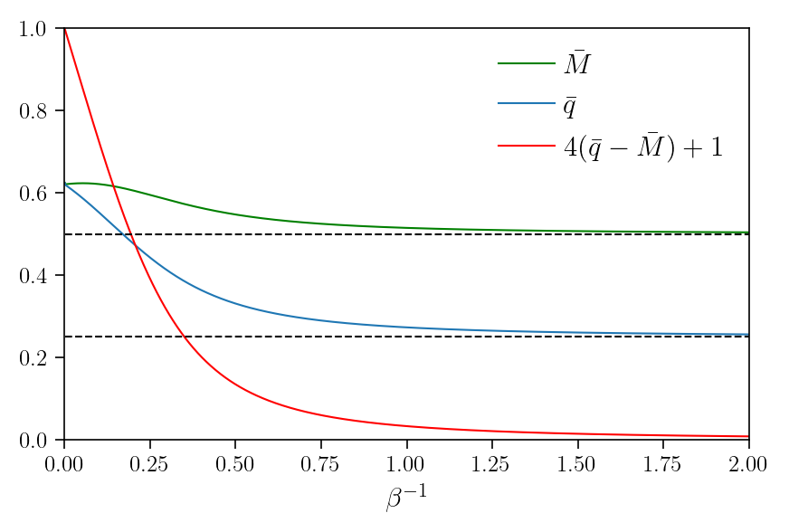
Figure 1: In this plot we show the behaviour of the mean value of the two replicas overlap $q_{12}$ (in blue) and the magnetization $q_{11}$ – whose mean value is denoted as $\bar{M}$– (in green) as found thanks to (45). Then, the linear combination that presents the expected behaviour is shown in red: it is equal to $1$ for small temperature and it cancels out for higher values of $T$. We stress that, unlike the SK model, in this case the transition is completely smooth.

Now, focusing on the linear susceptibility, we state that

$$\chi(M)=N\left(\langle M^{2}\rangle-\langle M\rangle^{2}\right)=\dfrac{1}{\beta^{2}}\partial^{2}_{H}\left(\dfrac{1}{N}\mathbb{E}_{\bm{J}}\log\mathcal{Z}(\beta,H)\right),$$ (46)

which can be computed as

$$\chi(M)=\dfrac{1}{2}\left[1-\mathbb{E}_{x}\tanh^{2}\left(\dfrac{\beta^{2}}{8}\left(\bar{M}-\bar{q}\right)+x\sqrt{\dfrac{\beta^{2}}{8}\bar{q}}+\beta\dfrac{H}{2}\right)\right].$$ (47)

Exploiting the relation

It is not cumbersome to compute the quenched average of the Hamiltonian as

$$\mathbb{E}\left[-\mathcal{H}_{N}\right]=\dfrac{\beta N}{4}\left(\langle M^{2}\rangle-\langle q_{12}^{2}\rangle\right)$$ (48)

and the derivative of the RS quenched statistical pressure with respect to $\beta$ as

$$N\partial_{\beta}A(\beta,H)=\dfrac{\beta N}{4}\left(\langle M\rangle^{2}-\langle q_{12}\rangle^{2}\right).$$ (49)

Since (48) and (49) are equal for definition, we get

$$N\left(\langle M\rangle^{2}-\langle M\rangle^{2}\right)=N\left(\langle q_{12}^{2}\rangle-\langle q_{12}\rangle^{2}\right)\Rightarrow\chi(M)=\chi(q_{12}).$$ (50)

In Fig. 2 we plot the behaviour of self-consistency equations (45) and the square root of the susceptibility for different values of the external field $H$. Instead, in Fig. 3 we show the behaviour of $\bar{M}$ via analytical computations, as in (56), and MC simulations, proving the goodness of our results.

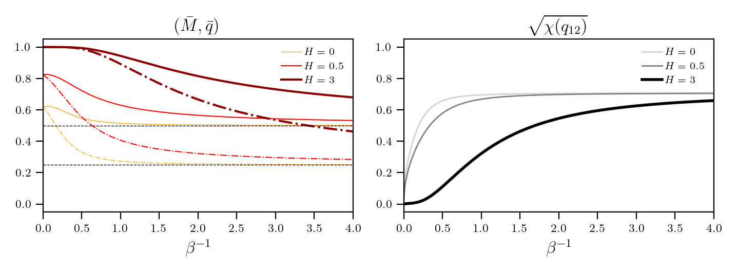
Figure 2: For different values of the external field $H$ we plot the values of self consistency equations (left) and square root of the susceptibility (right). In particular, we stress that, at $H$ increases, the values of the self-consistency equations ($\bar{M}$ solid lines, $\bar{q}$ dotted lines) improves and for low temperatures the square root of the susceptibility decreases, reaching the same plateau anyway at the value $\sqrt{\chi(q_{12})}=\sqrt{0.5}\approx 0.70$.

4.1 Computation of $\beta\to+\infty$ limit

Purpose of this Section is to analyze analytically the behaviour of the self-consistency equations in $\beta\to+\infty$, using the procedure introduced by Amit for Hopfield model Amit .

Let us start from the self-consistency equations, which are reported in the following for reader’s convenience

$$\begin{array}[]{lll}\bar{M}&=&\dfrac{1}{2}\left[1+\mathbb{E}_{x}\tanh\left(\dfrac{\beta^{2}}{8}\left(\bar{M}-\bar{q}\right)+x\sqrt{\dfrac{\beta^{2}}{8}\bar{q}}+\beta\dfrac{H}{2}\right)\right],\\ \\ \bar{q}&=&\bar{M}-\dfrac{1}{4}\left[1-\mathbb{E}_{x}\tanh^{2}\left(\dfrac{\beta^{2}}{8}\left(\bar{M}-\bar{q}\right)+x\sqrt{\dfrac{\beta^{2}}{8}\bar{q}}+\beta\dfrac{H}{2}\right)\right].\end{array}$$ (51)

If $\beta\to+\infty$ one can say that $\tanh^{2}(X)\to\textrm{sign}^{2}(X)=1$, so (51) becomes simply

$$\begin{array}[]{lll}\bar{q}&=&\bar{M}.\end{array}$$ (52)

Now, we can write $\bar{q}$ as

$$\begin{array}[]{lll}\bar{q}&=&\bar{M}-\dfrac{\delta{\bar{q}}}{\beta}\end{array}$$ (53)

and we add a generic term $\beta y/2$ in the argument of hyperbolic tangent in such a way that we can express the self-consistency equations as

$$\begin{array}[]{lll}\bar{M}&=&\dfrac{1}{2}\left[1+\mathbb{E}_{x}\tanh\left(\dfrac{\beta}{8}\delta{\bar{q}}+x\sqrt{\dfrac{\beta^{2}}{8}\left(\bar{M}-\dfrac{\delta{\bar{q}}}{\beta}\right)}+\beta\dfrac{H}{2}+\dfrac{\beta}{2}y\right)\right]\\ \\ \bar{M}-\dfrac{\delta{\bar{q}}}{\beta}&=&\bar{M}-\dfrac{1}{4}\left[1-\mathbb{E}_{x}\tanh^{2}\left(\dfrac{\beta}{8}\delta{\bar{q}}+x\sqrt{\dfrac{\beta^{2}}{8}\left(\bar{M}-\dfrac{\delta{\bar{q}}}{\beta}\right)}+\beta\dfrac{H}{2}+\dfrac{\beta}{2}y\right)\right].\end{array}$$ (54)

Then, if we derive $\bar{M}$ with respect to the auxiliary field $y$ we have

$$\begin{array}[]{lll}\partial_{y}\bar{M}&=&\dfrac{\beta}{2}\left[1-\mathbb{E}_{x}\tanh^{2}\left(\dfrac{\beta}{8}\delta{\bar{q}}+x\sqrt{\dfrac{\beta^{2}}{8}\left(\bar{M}-\dfrac{\delta{\bar{q}}}{\beta}\right)}+\beta\dfrac{H}{2}+\dfrac{\beta}{2}y\right)\right]=\delta\bar{q}\\ \\ \delta{\bar{q}}&=&\dfrac{\beta}{4}\left[1-\mathbb{E}_{x}\tanh^{2}\left(\dfrac{\beta}{8}\delta{\bar{q}}+x\sqrt{\dfrac{\beta^{2}}{8}\left(\bar{M}-\dfrac{\delta{\bar{q}}}{\beta}\right)}+\beta\dfrac{H}{2}+\dfrac{\beta}{2}y\right)\right].\end{array}$$ (55)

This allows us to perform explicitly $\beta\to\infty$ and we get

$$\begin{array}[]{lll}\bar{M}&=&\dfrac{1}{2}\left[1+\mathrm{erf}\left(\dfrac{\frac{1}{4}\delta{\bar{q}}+H+y}{\sqrt{\bar{M}}}\right)\right]\xrightarrow[]{y=0}\bar{M}=\dfrac{1}{2}\left[1+\mathrm{erf}\left(\dfrac{\delta{\bar{q}}+H}{4\sqrt{\bar{M}}}\right)\right]\,,\\ \\ \delta\bar{q}=\partial_{y}\bar{M}&=&\dfrac{1}{\sqrt{\pi\bar{M}}}\exp\left[-\dfrac{\left(\frac{1}{4}\delta{\bar{q}}+H+y\right)^{2}}{\bar{M}}\right]\xrightarrow[]{y=0}\delta\bar{q}=\dfrac{1}{\sqrt{\pi\bar{M}}}\exp\left[-\dfrac{\left(\delta{\bar{q}}+H\right)^{2}}{16\bar{M}}\right]\,.\end{array}$$ (56)

For $H=0$, we get $\bar{M}\approx 0.62$. This result is perfectly coherent with that one reached via MC simulation in Fig. 3.

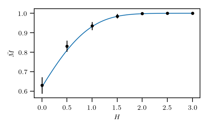
Figure 3: The comparison, at zero fast noise, namely $T=0$, between the self-consistency equation for $\bar{M}$ (56) (solid light-blue line) and MC simulations (black point) using updating rules derived in Subsec. 2.1 for different values of $H$. We stress that there is complete coherence between the analytical and numerical results.

Remark 2.

Having the expression of the quenched statistical pressure in the RS assumption, we can find the RS entropy of the model using the equation

$$s(T)=-\dfrac{\partial f}{\partial T}=\dfrac{1}{T^{2}}\dfrac{\partial f}{\partial\beta},$$ (57)

which gives us the following result

$$s^{\textnormal{RS}}(T)= \log 2+\dfrac{1}{8T^{2}}(\bar{M}-\bar{q})-\dfrac{3}{8T^{2}}(\bar{M}^{2}-\bar{q}^{2})-\dfrac{H}{2T}(2\bar{M}-1)$$

$$-\mathbb{E}_{x}\log\left\{\cosh\left[\dfrac{\beta^{2}}{8}\left(\bar{M}-\bar{q}\right)+x\sqrt{\dfrac{\beta^{2}}{8}\bar{q}}+\beta\dfrac{H}{2}\right]\right\}.$$ (58)

This expression is plotted in Fig. 4. As one can see, the entropy seems to be negative close to the zero-temperature: this cannot be possible since the entropy of a discrete system has to be always positive. Therefore, this suggests to change the assumption on the distribution of the order parameter, as already done for the SK model, in order to use the RSB framework. In this paper in Sec. 5.2 we will approach only the 1RSB one.

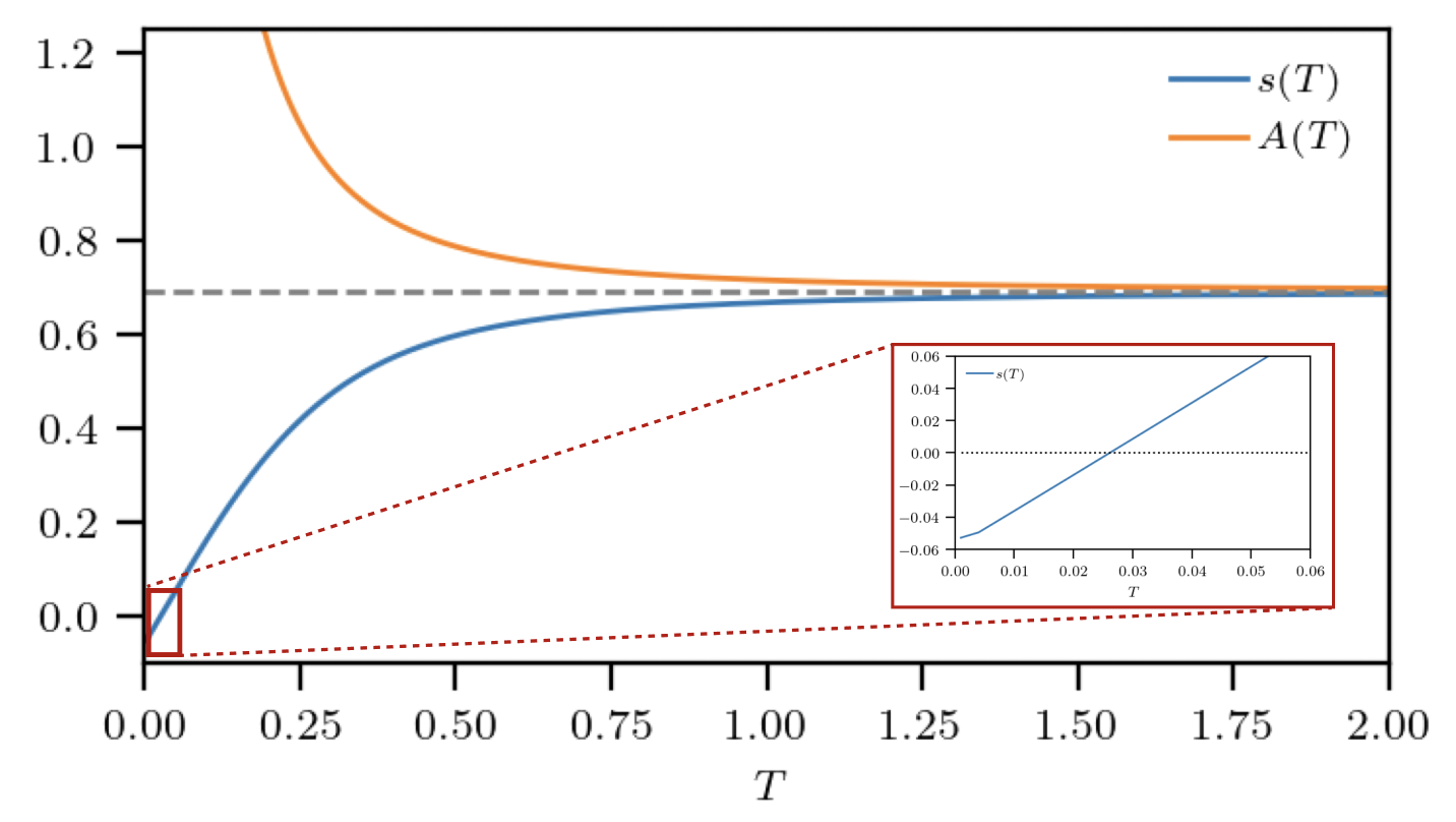
Figure 4: We plot the intensity entropy (in blue) and the intensity quenched statistical pressure (in orange) in RS assumption with respect to the temperature $T$. Both expressions show a plateau at $\log{2}$ for greater temperature, instead for smaller ones a zoom is shown and one can see that the entropy becomes negative. This suggest that the RS assumption for small vale of $T$ is not correct at all and this is a strong motivation for introducing the RSB framework.

5 Understanding the stability of RS assumption

The purpose of this section is twofold.
First, we wonder if it is possible to detect the transition between RS and 1RSB approximations for our model. To do so, we apply a new method introduced in albanese2023almeida for Hopfield model inspired to that one described by Toninelli in toninelli2002almeida for SK model.

However, unlike the classic method in de1978stability , we need to recover first the expression of the quenched statistical pressure (or equivalently the quenched free energy) for the 1RSB assumption, which takes us to the second aim of this Section. So, let us start with this results, obtained also in this case using Guerra’s interpolation.

Remark 3.

Before applying the RSB framework to solve the model, we wonder if it is the suitable one. Indeed, if we consider the expression of the Hamiltonian (1) with $H=0$ and $s_{i}\in\{0,1\}$, stressing that

$$s=\dfrac{1}{2}\left(\sigma-1\right),\quad\sigma\in\{-1,+1\},\ s\in\{0,1\},$$ (59)

we get that

$$\mathcal{H}_{N}(\bm{s}|\bm{J})= -\dfrac{1}{2\sqrt{N}}\sum_{i<j}J_{ij}\left[\dfrac{1}{4}\left(\sigma_{i}-1\right)\left(\sigma_{j}-1\right)\right]$$

$$=-\dfrac{1}{8\sqrt{N}}\sum_{i<j}J_{ij}\sigma_{i}\sigma_{j}+\dfrac{1}{4\sqrt{N}}\sum_{i<j}J_{ij}\sigma_{i}-\dfrac{1}{8\sqrt{N}}\sum_{i<j}J_{ij}$$

$$=-\dfrac{1}{4}\mathcal{H}_{N}(\bm{\sigma}|J)+\dfrac{1}{4}\sum_{i=1}^{N}h_{i}\sigma_{i}-\dfrac{1}{8\sqrt{N}}\sum_{i<j}J_{ij},$$ (60)

where we use $h_{i}=\dfrac{1}{\sqrt{N}}\sum_{j}J_{ij}$ where $h_{i}\sim\mathcal{N}(0,1)$. In this way we can easily see that the Ising and Boolean spins models differs only for a one body term, for which self-averaging as proven in App. B, and a factor which is independent from the spin configuration ($(8\sqrt{N})^{-1}\sum_{i<j}J_{ij}$). Therefore, the self averaging of the free energy and the possibility to use the RSB framework are completely justified.

From this we inherit a new set of Ghirlanda Guerra equalities ghirlanda1998general which can be apply to the model, as proven in App. C:

$$\left\langle\left(q_{12}^{2}-q_{13}^{2}\right)^{2}\right\rangle-\left\langle\left(q_{11}^{2}-q_{13}^{2}\right)^{2}\right\rangle+\Big{(}\left\langle q_{11}^{2}\right\rangle-\left\langle q_{12}^{2}\right\rangle\Big{)}^{2}=0$$ (61)

We stress that in classic SK case, we have that $q_{11}=1$ and (61) takes to the classic Ghirlanda Guerra identity:

$$\langle q_{12}^{4}\rangle-2\langle q_{12}^{2}q_{13}^{2}\rangle+\langle q_{12}^{2}\rangle^{2}=0,$$ (62)

as shown always in App. C.

In order to double check this we have proved numerically the correctness of (61) and the result is shown in Figure 5. Particularly, we stress that the new Ghirlanda Guerra (61) goes to zero quickly for small size network $N$ already.

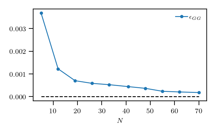
Figure 5: Value of the right hand side term of Eq. (61) with respect to the size of the network $N$. We stress that it is perfectly coherent with the theoretical results and it goes to zero very quickly, also for small sizes of the network $N$.

5.1 Guerra’s interpolation: 1RSB assumption

Now we solve the model via Guerra’s interpolation in 1RSB assumption. This means that the probability distribution of the order parameter $q_{ab}$, when the two replicas are different, displays two peaks in $\bar{q}_{1}$ and $\bar{q}_{2}$ concentrated with respect to a parameter $\theta\in[0,1]$

$$\mathbb{P}(\bm{s})=\lim_{N\to+\infty}\mathbb{E}_{\bm{J}}\mathbb{P}_{N,J}(\bm{s})=\delta_{ab}\delta(q_{ab}-\bar{M})+(1-\delta_{ab})\left((1-\theta)\delta(q_{ab}-\bar{q}_{2})+\theta\delta(q_{ab}-\bar{q}_{1})\right).$$ (63)

Let $t$ the real positive interpolating parameter, $Y_{i}^{(a)}\sim\mathcal{N}(0,1),$ $a=1,2$ auxiliary Gaussian field i.i.d. and $A^{(1)},\ A^{(2)},B$ constants to be set a posteriori. The interpolating partition function $Z_{N}(t|\beta)$ can be written, as explained by Guerra in guerra_broken , in such a way that we need to define first $Z_{2}(t|\beta)$

$$Z_{2}(t|\beta)=\sum_{\{\bm{s}\}}\exp\left[\sqrt{t}\dfrac{\beta}{2\sqrt{N}}\displaystyle\sum\limits_{i<j}^{N}J_{ij}s_{i}s_{j}+\sqrt{1-t}\sum_{a=1}^{2}A^{(a)}\displaystyle\sum\limits_{i=1}^{N}Y_{i}^{(a)}s_{i}+(1-t)B\displaystyle\sum\limits_{i=1}^{N}s_{i}+\beta H\displaystyle\sum\limits_{i=1}^{N}s_{i}\right].$$ (64)

Then, we average out the fields one per time in order to get

$$Z_{1}(t|\beta)\coloneqq \left[\mathbb{E}_{2}Z_{2}(t|\beta)^{\theta}\right]^{1/\theta}$$ (65)

$$Z_{0}(t|\beta)\coloneqq \exp\left\{\mathbb{E}_{1}\left[\log Z_{1}(t|\beta)\right]\right\}$$ (66)

$${Z}_{N}(t|\beta)\coloneqq Z_{0}(t|\beta),$$ (67)

where $\mathbb{E}_{a}$ is the average with respect to all the i.i.d. $Y_{i}^{(a)}$.

The interpolating quenched statistical pressure is introduced as

$$\mathcal{A}_{N}(\beta)=\dfrac{1}{N}\mathbb{E}_{0}\log Z_{N}(t|\beta),$$ (68)

where $\mathbb{E}_{0}$ represents the average with respect to all the i.i.d. $J_{ij}$. In the thermodynamic limit, we write

$$\mathcal{A}(\beta)=\lim_{N\to+\infty}\mathcal{A}_{N}(\beta).$$ (69)

Now, following Guerra’s prescription guerra_broken , given two copies (or replicas) of the system, we define the following averages, corresponding to thermalization within the two different levels of the hierarchy

$$\langle\cdot\rangle_{t,1}\coloneqq\mathbb{E}_{0}\mathbb{E}_{1}[\mathbb{E}_{2}\mathcal{W}_{2,t}\omega_{t}(\cdot)]^{2},$$ (70)

$$\langle\cdot\rangle_{t,2}\coloneqq\mathbb{E}_{0}\mathbb{E}_{1}\mathbb{E}_{2}\mathcal{W}_{2,t}[\omega_{t}(\cdot)]^{2},$$ (71)

where

$$\mathcal{W}_{2,t}\coloneqq\dfrac{{Z}_{2}^{\theta}(t|\beta)}{\mathbb{E}_{2}{Z}^{\theta}_{2}(t|\beta)}.$$ (72)

From now on, we imply the dependence on $t$ from the quenched average.

The purpose now is also in this case to apply the Fundamental Theorem of Calculus (34), so the next step is to compute the one body term and the derivative with respect to the interpolating parameter $t$. We start from the latter, reads as

$$d_{t}\mathcal{A}_{N}(t|\beta)= \dfrac{\beta^{2}}{8}\left[\langle q_{11}^{2}\rangle-(1-\theta)\langle q_{12}^{2}\rangle_{2}-\theta\langle q_{12}^{2}\rangle_{1}\right]-\dfrac{A^{(1)}}{2}\left[\langle q_{11}\rangle-(1-\theta)\langle q_{12}\rangle_{2}-\theta\langle q_{12}\rangle_{1}\right]$$

$$-\dfrac{A^{(1)}}{2}\left[\langle q_{11}\rangle-(1-\theta)\langle q_{12}\rangle_{2}\right]-B\langle q_{11}\rangle.$$ (73)

Since the recovery of this expression is a straightforward generalization of that one in RS assumption, it is left to the reader.

Thanks to 1RSB assumption, we state that

$$\langle(q_{12}-\bar{q})^{2}\rangle_{a}\to 0,\quad a=1,2\quad\quad\langle(q_{11}-\bar{M})^{2}\rangle\to 0,\quad\textnormal{as}\ N\to+\infty.$$ (74)

Therefore,

$$\langle(q_{12}-\bar{q})^{2}\rangle_{a}= \langle q_{12}^{2}\rangle+\bar{q}^{2}-2\bar{q}\langle q_{12}\rangle\to 0,\quad a=1,2$$ (75)

$$\langle(q_{11}-\bar{M})^{2}\rangle= \langle q_{11}^{2}+\bar{M}^{2}-2\bar{M}\langle q_{11}\rangle\to 0.$$ (76)

Replacing $\langle q_{11}^{2}\rangle$, $\langle q_{12}^{2}\rangle_{1}$ and $\langle q_{12}^{2}\rangle_{2}$ using (75) and (76) and defined $A^{(1)}$, $A^{(2)}$ and $B$ in such a way that

$$\begin{array}[]{lll}(A^{(1)})^{2}=\dfrac{\beta^{2}}{2}\bar{q}_{1},&&(A^{(1)})^{2}=\dfrac{\beta^{2}}{2}\left(\bar{q}_{2}-\bar{q}_{1}\right),\quad B=\dfrac{\beta^{2}}{4}\left(\bar{M}-\bar{q}_{2}\right),\end{array}$$ (77)

we give the expression of the derivative with respect to $t$ of the interpolating quenched statistical pressure in the thermodynamic limit

$$\begin{array}[]{lll}d_{t}{A}(\beta,t)&=&-\dfrac{\beta^{2}}{8}\left[\bar{M}^{2}-(1-\theta)\bar{q}_{2}^{2}-\theta\bar{q}_{1}^{2}\right].\end{array}$$ (78)

Now the one body term is all we need. We report only the expression

$$\mathcal{A}(t=0|\beta)=\log 2+\dfrac{1}{\theta}\mathbb{E}_{1}\log\mathbb{E}_{2}\exp\left({\theta}g(\beta,\bm{Y})\right)\cosh^{\theta}g(\beta,\bm{Y})$$ (79)

where

$$g(\beta,\bm{Y})=\left[\dfrac{1}{2}\left(A^{(1)}Y^{(1)}+A^{(2)}Y^{(2)}+B+\beta H\right)\right].$$ (80)

Finally, putting together (78) and (79), we state the following

Theorem 3.

The quenched statistical pressure in 1RSB assumption and in the thermodynamic limit of the Boolean SK model is

$$\begin{array}[]{lll}\mathcal{A}_{\theta}(\beta)&=&\log 2+\dfrac{1}{\theta}\mathbb{E}_{1}\log\mathbb{E}_{2}e^{\theta g(\beta,\bm{Y})}\cosh^{\theta}\Big{[}g(\beta,\bm{Y})\Big{]}-\dfrac{\beta^{2}}{8}\Big{(}\bar{M}^{2}-\bar{q}^{2}_{2}\Big{)}-\theta\dfrac{\beta^{2}}{8}\Big{(}\bar{q}^{2}_{2}-\bar{q}_{1}^{2}\Big{)}\end{array}$$ (81)

where

$$g(\beta,\bm{Y})=\dfrac{\beta^{2}}{8}(\bar{M}-\bar{q}_{2})+Y^{(1)}\sqrt{\dfrac{\beta^{2}}{8}\bar{q}_{1}}+Y^{(2)}\sqrt{\dfrac{\beta^{2}}{8}(\bar{q}_{2}-\bar{q}_{1})}.$$ (82)

The order parameters fulfill the following self-consistency equations

$$\begin{array}[]{lll}\bar{M}=\dfrac{1}{2}\left[1+\mathbb{E}_{1}\left\{\dfrac{\mathbb{E}_{2}e^{\theta g(\beta,\bm{Y})}\cosh^{\theta}\Big{[}g(\beta,\bm{Y})\Big{]}\tanh\Big{[}g(\beta,\bm{Y})\Big{]}}{\mathbb{E}_{2}e^{\theta g(\beta,\bm{Y})}\cosh^{\theta}\Big{[}g(\beta,\bm{Y})\Big{]}}\right\}\right],\\ \\ \bar{q}_{2}=M+\dfrac{1}{4}\left[\mathbb{E}_{1}\left\{\dfrac{\mathbb{E}_{2}e^{\theta g(\beta,\bm{Y})}\cosh^{\theta}\Big{[}g(\beta,\bm{Y})\Big{]}\tanh^{2}\Big{[}g(\beta,\bm{Y})\Big{]}}{\mathbb{E}_{2}e^{\theta g(\beta,\bm{Y})}\cosh^{\theta}\Big{[}g(\beta,\bm{Y})\Big{]}}\right\}-1\right],\\ \\ \bar{q}_{1}=M+\dfrac{1}{4}\left[\mathbb{E}_{1}\left\{\dfrac{\mathbb{E}_{2}e^{\theta g(\beta,\bm{Y})}\cosh^{\theta}\Big{[}g(\beta,\bm{Y})\Big{]}\tanh\Big{[}g(\beta,\bm{Y})\Big{]}}{\mathbb{E}_{2}e^{\theta g(\beta,\bm{Y})}\cosh^{\theta}\Big{[}g(\beta,\bm{Y})\Big{]}}\right\}^{2}-1\right].\end{array}$$ (83)

Remark 4.

We stress that if we put $\theta=0$ or $\theta=1$ in the expression of the 1RSB approximation of the quenched statistical pressure (81) we come back to that one in RS assumption (44) .
Indeed, for $\theta=0$ we get

$$\begin{array}[]{lll}\mathcal{A}_{\theta=0}(\beta)&=&\log 2+\mathbb{E}_{1}\mathbb{E}_{2}\left[g(\beta,\bm{Y})+\log\cosh\Big{[}g(\beta,\bm{Y})\Big{]}\right]-\dfrac{\beta^{2}}{8}\Big{(}\bar{M}^{2}-\bar{q}^{2}_{2}\Big{)}\\ \\ &=&\log 2+\mathbb{E}_{x}\log\cosh\Big{[}g(\beta,x)\Big{]}+\dfrac{\beta^{2}}{8}(\bar{M}-\bar{q}_{2})-\dfrac{\beta^{2}}{8}\Big{(}\bar{M}^{2}-\bar{q}^{2}_{2}\Big{)}=\mathcal{A}^{RS}(\beta)\end{array}$$ (84)

where

$$g(\beta,x)=\dfrac{\beta^{2}}{8}(\bar{M}-\bar{q}_{2})+x\sqrt{\dfrac{\beta^{2}}{8}\bar{q}_{2}}.$$ (85)

Instead, for $\theta=1$ we have that

$$\begin{array}[]{lll}\mathcal{A}_{\theta=1}(\beta)&=&\log 2+\mathbb{E}_{1}\log\mathbb{E}_{2}e^{g(\beta,\bm{Y})}\cosh\Big{[}g(\beta,\bm{Y})\Big{]}-\dfrac{\beta^{2}}{8}\Big{(}\bar{M}^{2}-\bar{q}^{2}_{1}\Big{)}.\end{array}$$ (86)

Focusing on the integral in $\mathbb{E}_{2}$ we get that

$$\begin{array}[]{lll}\mathbb{E}_{2}e^{g(\beta,\bm{Y})}\cosh\Big{[}g(\beta,\bm{Y})\Big{]}&=&\dfrac{1}{2}+\dfrac{1}{2}\mathbb{E}_{2}\left(e^{2g(\beta,\bm{Y})}\right)\\ \\ &=&\dfrac{1}{2}\left(1+\exp\left[\dfrac{\beta^{2}}{4}(\bar{M}-\bar{q}_{1})+Y^{(1)}2\sqrt{\dfrac{\beta^{2}}{8}\bar{q}_{1}}\right]\right)\\ \\ &=&\exp\left[\dfrac{\beta^{2}}{8}(\bar{M}-\bar{q}_{1})+Y^{(1)}\sqrt{\dfrac{\beta^{2}}{8}\bar{q}_{1}}\right]\cosh\left(\dfrac{\beta^{2}}{8}(\bar{M}-\bar{q}_{1})+Y^{(1)}\sqrt{\dfrac{\beta^{2}}{8}\bar{q}_{1}}\right),\end{array}$$ (87)

thus

$$\begin{array}[]{lll}\mathcal{A}_{\theta=1}(\beta)&=&\log 2+\dfrac{\beta^{2}}{8}(\bar{M}-\bar{q}_{1})+\mathbb{E}_{x}\log\cosh\Big{[}g^{RS}(\beta,x)\Big{]}-\dfrac{\beta^{2}}{8}\Big{(}\bar{M}^{2}-\bar{q}^{2}_{1}\Big{)}=\mathcal{A}^{RS}(\beta).\end{array}$$ (88)

5.2 AT line for Boolean SK

Now that we have the expression of the quenched statistical pressure in 1RSB assumption, we can check the stability of the two assumptions with respect to different values of the temperature.

Our method is based on the fact that, for $\theta\in\{0,1\}$ one of the two-delta peaks in 1RSB assumption vanishes and the 1RSB expression of the quenched free energy naturally becomes the RS one.

Then, we prove that for values of $\theta$ close but away from one, the 1RSB expression of the quenched free energy is smaller than the RS expression, i.e. $f_{1RSB}(\bar{M},\bar{q}_{2},\bar{q}_{1}|\theta)<f_{RS}(\bar{m},\bar{q})$, below a critical line in $\beta$, known as AT line.

Therefore, we expand the 1RSB quenched free-energy around $\theta=1$ to the first order, namely

$$f_{1RSB}({\bar{M},\,}\bar{q}_{2},\bar{q}_{1}|\theta)= f_{1RSB}({\bar{M},\,}\bar{q}_{2},\bar{q}_{1}|\theta)|_{\theta=1}+(\theta-1)\partial_{\theta}f_{1RSB}({\bar{M},\,}\bar{q}_{2},\bar{q}_{1}|\theta)|_{\theta=1},$$ (89)

where $f_{1RSB}({\bar{M},\,}\bar{q}_{2},\bar{q}_{1}|\theta)|_{\theta=1}=f_{RS}({\bar{M},\,}\bar{q})$. To determine when the RS solution becomes unstable, i.e. $f_{1RSB}({\bar{M},\,}\bar{q}_{2},\bar{q}_{1}|\theta)<f_{RS}({\bar{M},\,}\bar{q})$ we inspect the sign of $\partial_{\theta}f_{1RSB}({\bar{M},\,}\bar{q}_{2},\bar{q}_{1}|\theta)|_{\theta=1}$, keeping in mind that $\theta-1<0$.

Since the 1RSB self-consistency equations (83) also depend on $\theta$, we need to expand them with respect to $\theta$ around one too:

$$\bar{M}= \bar{M}^{(RS)}+(\theta-1)A(\bar{M},\bar{q}_{1},\bar{q}_{2})$$ (90)

$$\bar{q}_{1}= \bar{q}^{(RS)}+(\theta-1)B(\bar{M},\bar{q}_{1},\bar{q}_{2})$$ (91)

$$\bar{q}_{2}= \tilde{q}_{2}+(\theta-1)C(\bar{M},\bar{q}_{1},\bar{q}_{2}),$$ (92)

where $\bar{M}^{(RS)}$ and $\bar{q}^{(RS)}$ fulfill the RS self-consistency equations (45) and $\tilde{q}_{2}$ is the solution of the following self-consistency equation

$$\tilde{q}_{2}=\mathbb{E}_{1}\left[\dfrac{\mathbb{E}_{2}e^{g(\bar{M},\bar{q}_{2},\bar{q}_{1})}\cosh g(\bar{M},\bar{q}_{2},\bar{q}_{1})\tanh^{2}g(\bar{M},\bar{q}_{2},\bar{q}_{1})}{\mathbb{E}_{2}e^{g(\bar{M},\bar{q}_{2},\bar{q}_{1})}\cosh g(\bar{M},\bar{q}_{2},\bar{q}_{1})}\right].$$ (93)

The expression of $A(\bar{M},\bar{q}_{2},\bar{q}_{1}),\ B(\bar{M},\bar{q}_{2},\bar{q}_{1})$ and $C(\bar{M},\bar{q}_{2},\bar{q}_{1})$ are reported in Appendix D. From now on, we imply the apex $(RS)$ on $\bar{q}$ and $\bar{M}$

The derivative of the 1RSB quenched statistical pressure with respect to $\theta$, when $\theta=1$ is

$$K(\bar{M},\bar{q},\tilde{q}_{2})=\partial_{\theta}\left(-\beta f_{1RSB}({\bar{M},\,}\bar{q}_{2},\bar{q}_{1}|\theta)\right)|_{\theta=1}=-\dfrac{\beta^{2}}{8}\left(\tilde{q}_{2}^{2}-\bar{q}^{2}\right)+\dfrac{\beta^{2}}{8}\left(\bar{M}-\tilde{q}_{2}\right)+\dfrac{\beta^{2}}{4}\bar{M}(\tilde{q}_{2}-\bar{q})$$

$$-\mathbb{E}_{1}\log\mathbb{E}_{2}e^{g(\bar{M},\tilde{q}_{2},\bar{q})}\cosh g(\bar{M},\tilde{q}_{2},\bar{q})+\mathbb{E}_{1}\dfrac{\mathbb{E}_{2}e^{g(\bar{M},\tilde{q}_{2},\bar{q})}\cosh g(\bar{M},\tilde{q}_{2},\bar{q})\log\cosh g(\bar{M},\tilde{q}_{2},\bar{q})}{\mathbb{E}_{2}e^{g(\bar{M},\tilde{q}_{2},\bar{q})}\cosh g(\bar{M},\tilde{q}_{2},\bar{q})}.$$ (94)

We notice that, for $\tilde{q}_{2}=\bar{q}$, $K(\bar{M},\bar{q},\bar{q})=0$ and we study the behaviour of the function $K({\bar{M},\,}\bar{q},x)$ for $x\in[0,\bar{q}]$. For $x=\bar{q}$, independently from $\bar{M}$, we have $K({\bar{M},\,}\bar{q},\bar{q})=0$, while the extremum of $K({\bar{M},\,}\bar{q},x)$ is found from

$$\partial_{x}K({\bar{M},\,}\bar{q},x) =-\dfrac{\beta^{2}}{4}x-\dfrac{\beta^{2}}{16}+\dfrac{\beta^{2}}{4}\bar{M}+\dfrac{\beta^{2}}{16}\mathbb{E}_{1}\left[\dfrac{\mathbb{E}_{2}e^{g(\bar{M},x,\bar{q}_{1})}\cosh g(\bar{M},x,\bar{q}_{1})\tanh^{2}g(\bar{M},x,\bar{q}_{1})}{\mathbb{E}_{2}e^{g(\bar{M},x,\bar{q}_{1})}\cosh g(\bar{M},x,\bar{q}_{1})}\right]$$ (95)

which is null when $x=\tilde{q}_{2}(\bar{M},\bar{q})$.

Supposing the extremum global and considering that $K(\bar{M},\bar{q},\bar{q})=0$, if $x=\tilde{q}_{2}$ is a minimum, then $K(\bar{M},\bar{q},\tilde{q}_{2})<0$. Therefore, computing the second derivative with respect to $x$ we get

$$\partial_{x^{2}}K({\bar{M},\,}\bar{q},x) =-\dfrac{\beta^{2}}{4}\left(1-\dfrac{\beta^{2}}{32}\mathbb{E}_{1}\left[\dfrac{\mathbb{E}_{2}e^{g(\bar{M},\tilde{q}_{2},\bar{q})}\cosh g(\bar{M},\tilde{q}_{2},\bar{q})\textnormal{sech}^{3}g(\bar{M},\tilde{q}_{2},\bar{q})}{\mathbb{E}_{2}e^{g(\bar{M},\tilde{q}_{2},\bar{q})}\cosh g(\bar{M},\tilde{q}_{2},\bar{q})}\right]\right)$$ (96)

which is positive when

$$1-\dfrac{\beta^{2}}{32}\mathbb{E}_{1}\left[\dfrac{\mathbb{E}_{2}e^{g(\bar{M},\tilde{q}_{2},\bar{q})}\cosh g(\bar{M},\tilde{q}_{2},\bar{q})\textnormal{sech}^{3}g(\bar{M},\tilde{q}_{2},\bar{q})}{\mathbb{E}_{2}e^{g(\bar{M},\tilde{q}_{2},\bar{q})}\cosh g(\bar{M},\tilde{q}_{2},\bar{q})}\right]<0.$$ (97)

Hence the RS theory becomes unstable when the expression in (97) becomes negative, which in the $\tilde{q}_{2}\to\bar{q}$ limit becomes the corresponding of the well-known AT line for the SK model

$$1-\dfrac{\beta^{2}}{32}\mathbb{E}_{x}\left[{\textnormal{sech}^{4}\left(\dfrac{\beta^{2}}{8}(\bar{M}-\bar{q})+x\sqrt{\dfrac{\beta^{2}}{8}\bar{q}}\right)}\right]<0.$$ (98)

In Fig. 6 we show for which values of $\bar{M}$, $\bar{q}_{1}$ and $\bar{q}_{2}$ the AT line (98) is fulfilled. We notice that, apart from small values of $T$, the RS solutions seems to well approximate the model. In the zoom it is possible to better see the difference between $\bar{q}_{1}$ and $\bar{q}_{2}$ for small temperatures.

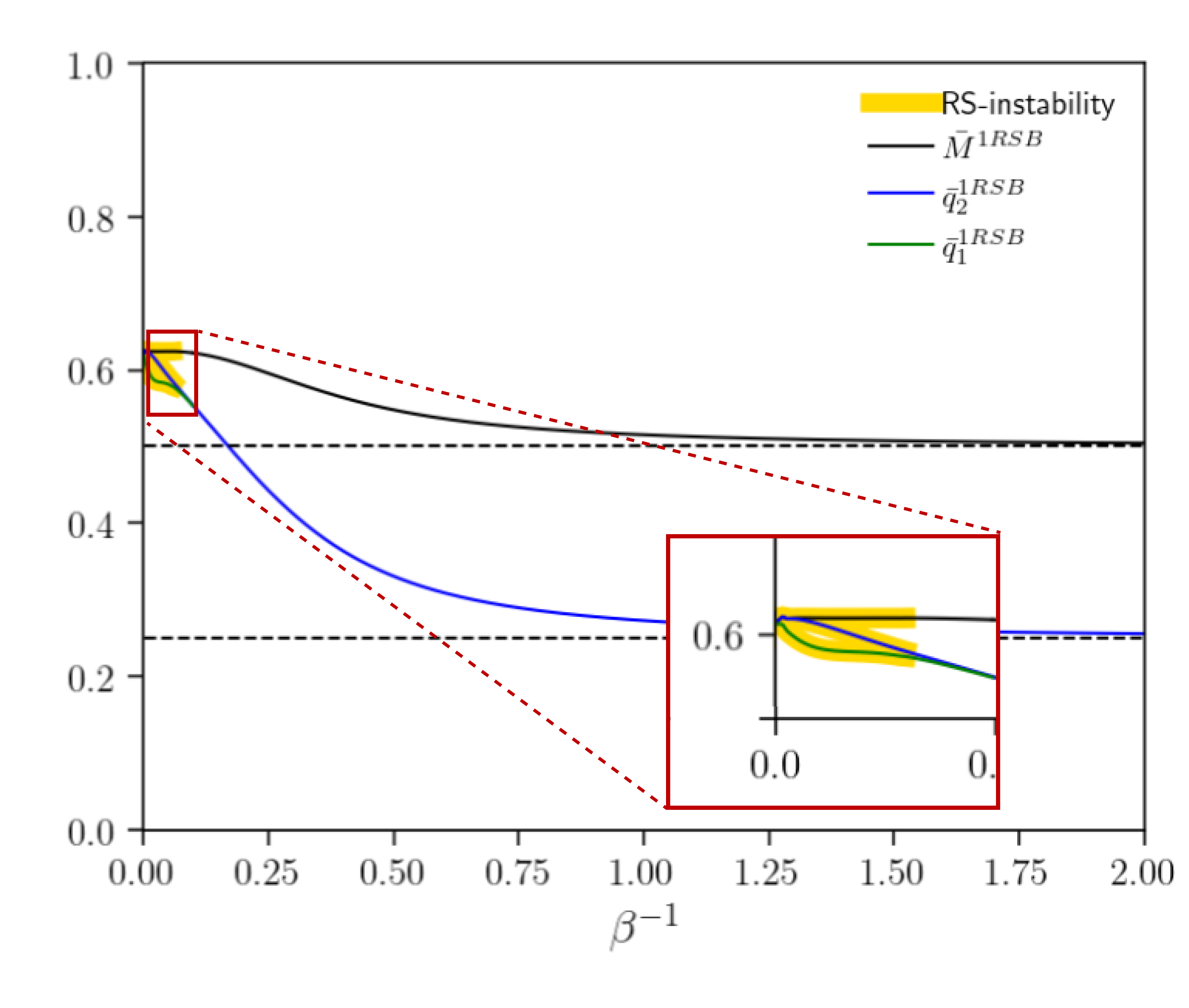
Figure 6: Numerical computation of the self-consistency equations (83). The part underlined in yellow is zoomed in the red square and represents the instability of the RS assumption recovered by AT line (98). We notice that the $\bar{q}_{1}$ and $\bar{q}_{2}$ are different only when the RS is unstable, as expected.

Remark 5.

After the computation of the expression of the quenched statistical pressure of the Boolean SK model we can easily compute the entropy also in this assumption using Eq. (57), reads as

$$s(T)= \log 2+\dfrac{1}{8T^{2}}(\bar{M}^{2}-\bar{q_{2}}^{2})+\dfrac{\theta}{8T^{2}}(\bar{q}_{2}^{2}-\bar{q}_{1}^{2})+\dfrac{1}{\theta}\mathbb{E}_{1}\log\mathbb{E}_{2}e^{\theta g(\beta,\bm{Y})}\cosh^{\theta}\Big{[}g(\beta,\bm{Y})\Big{]}$$

$$+\dfrac{1}{2T^{2}}\bar{M}(\bar{M}-\bar{q}_{2})-\dfrac{\theta\bar{q}_{1}}{8T^{2}}\left(4(\bar{q}_{1}-\bar{M})+1\right)+\dfrac{\bar{q}_{2}}{8T^{2}}+\dfrac{\bar{q}_{2}}{8T^{2}}(\theta-1)\left(4(\bar{q}_{2}-M)+1\right)$$

$$+\dfrac{\theta}{8T^{2}}(\bar{q}_{2}-\bar{q}_{1})+\dfrac{\theta}{8T^{2}}(2\bar{M}-1)(\bar{q}_{2}-\bar{q}_{1}).$$ (99)

The numerical result both for RS and 1RSB approximations are shown in Figure 7. We notice that latter has a better behaviour with respect to the former and, in particular, the AT line foresees perfectly the passage from RS to 1RSB.

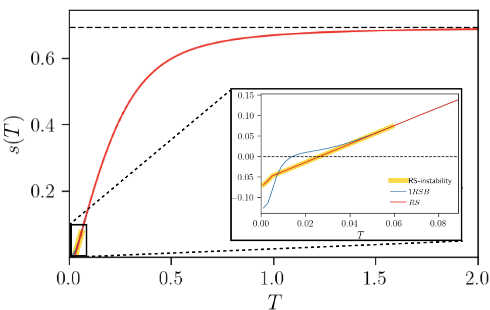
Figure 7: The numerical computation of the entropy for RS (red) and 1RSB (blue) assumptions. The yellow line represents the RS instability computed through AT line. We have also zoomed the plot in order to show the difference between the two assumptions for small temperature. As we can see from the zoom in the small temperature region, the 1RSB assumption improve the region of validity of the solution, as the intesity entropy becomes negative for smaller value of temperature with respect the RS solution.

6 Conclusions and outlooks

In this work we have devise some analytical and numerical results regarding a mean field network called Boolean SK model. This is made of $N$ Ising spins which can assume values $\{0,\ 1\}$ whose connections are random i.i.d. standard Gaussian variables. The name comes to the fact that the Hamiltonian of the model is the same for the SK model sherrington1975solvable . One of the main purposes was to create a framework, inspired to that one from SK model, to solve the model in the thermodynamic limit. This may prove useful with a view to linking the statistical mechanics of spin glass to ML models, which routinely use variables of $\{0,1\}$ type.

To do so, we have proven, using Guerra and Toninelli’s approach guerra2002thermodynamic , in that limit the existence and uniqueness of the quenched statistical pressure of the Boolean SK model. Moreover we have devised it in RS and 1RSB assumptions, applying Guerra’s interpolation. This method is mathematically rigorous and justified in every passage and allows us to come to the expressions without using the much more common replica trick that is nevertheless heuristic. There is complete coherence between the RS and 1RSB expression, proving the goodness of the method.

The corresponding of the AT line de1978stability was computed and we notice numerically that the RS approximation is unstable only for a limited number of values of temperature, the smaller ones. This leads us to believe that RS assumption is a good approximation to solve the model.

Our results are corroborated in the paper via numerical approach, showing the perfect coincidence with the analytical expressions.

Future outlooks could be using Boolean variables also for other typologies of models, such as associative neural networks Hopfield ; Amit , in order to understand what kind of changes in the collective properties there may be.

Appendix A Computations of the derivative with respect to $t$

In this Appendix we report the computations to recover the expression of the derivative with respect to the interpolating parameter $t$ of the interpolating quenched statistical pressure.

$$d_{t}A_{N}(t|\beta)= \dfrac{1}{N}\mathbb{E}\dfrac{1}{Z_{N}(t|\beta)}\sum_{\{\bm{s}\}}B_{N}(\bm{s}|\bm{J})\left(\dfrac{\beta}{4\sqrt{Nt}}\sum_{i,j=1}^{N}J_{ij}s_{i}s_{j}-\dfrac{A}{2\sqrt{1-t}}\sum_{i=1}^{N}Y_{i}s_{i}-B\sum_{i=1}^{N}s_{i}\right)$$ (100)

$$= \dfrac{\beta}{2\sqrt{Nt}N}\sum_{i,j=1}^{N}\mathbb{E}\partial_{J_{ij}}\left(\omega(s_{i}s_{j})\right)-\dfrac{A}{2N\sqrt{1-t}}\sum_{i=1}^{N}\mathbb{E}\partial_{Y_{i}}\left(\omega(s_{i})\right)-\dfrac{B}{N}\sum_{i=1}^{N}\mathbb{E}\omega(s_{i}),$$ (101)

where in the last passage we have applied Stein’s Lemma (22).

The computations of the partial derivatives with respect to $J_{ij}$ and $Y_{i}$ are similar. For this reason we show only the former:

$$\mathbb{E}\partial_{J_{ij}}\left(\omega(s_{i}s_{j})\right)= \dfrac{\beta}{4\sqrt{Nt}N}\sum_{i,j=1}^{N}\mathbb{E}\dfrac{1}{Z_{N}(t|\beta)}\partial_{J_{ij}}\left(\sum_{\{\bm{s}\}}B_{N}(\bm{s}|\bm{J})s_{i}s_{j}\right)$$

$$-\dfrac{\beta}{4\sqrt{Nt}N}\sum_{i,j=1}^{N}\mathbb{E}\partial_{J_{ij}}\left(\dfrac{1}{Z_{N}(t|\beta)}\right)\sum_{\{\bm{s}\}}B_{N}(\bm{s}|\bm{J})s_{i}s_{j}$$ (102)

$$= \dfrac{\beta}{4\sqrt{Nt}N}\sum_{i,j=1}^{N}\mathbb{E}\dfrac{1}{Z_{N}(t|\beta)}\sum_{\{\bm{s}\}}B_{N}(\bm{s}|\bm{J})s_{i}s_{j}\left(\dfrac{\beta\sqrt{t}}{2\sqrt{N}}s_{i}s_{j}\right)$$

$$-\dfrac{\beta}{4\sqrt{Nt}N}\sum_{i,j=1}^{N}\mathbb{E}-\dfrac{1}{Z_{N}^{2}(t|\beta)}\partial_{J_{ij}}\left(Z_{N}(t|\beta)\right)\sum_{\{\bm{s}\}}B_{N}(\bm{s}|\bm{J})s_{i}s_{j}$$ (103)

$$= \dfrac{\beta}{4\sqrt{Nt}N}\sum_{i,j=1}^{N}\mathbb{E}\dfrac{1}{Z_{N}(t|\beta)}\sum_{\{\bm{s}\}}B_{N}(\bm{s}|\bm{J})s_{i}s_{j}\left(\dfrac{\beta\sqrt{t}}{2\sqrt{N}}s_{i}s_{j}\right)$$

$$-\dfrac{\beta}{4\sqrt{Nt}N}\sum_{i,j=1}^{N}\mathbb{E}-\dfrac{1}{Z_{N}^{2}(t|\beta)}\left(\sum_{\{\bm{s}\}}B_{N}(\bm{s}|\bm{J})s_{i}s_{j}\right)^{2}\dfrac{\beta\sqrt{t}}{2\sqrt{N}}$$ (104)

which takes us to the expression in (35).

Appendix B Self-averaging for one body Hamiltonian

In this Appendix we show that the model whose Hamiltonian is

$$\mathcal{H}^{1-body}_{N}=\sum_{i=1}^{N}h_{i}s_{i},$$ (105)

where $h_{i}\sim\mathcal{N}(0,1)$ and $s_{i}\in\{0,1\},$ for $i=1,\ldots,N$, fulfills the self-averaging property. To do so, we have that the normalised variance of the intensive energy $u=\dfrac{1}{N}\mathcal{H}^{1-body}_{N}$ tends to zero in the thermodynamic limit

$$\dfrac{\sqrt{\mathrm{Var}(u)}}{\langle u\rangle}\to 0,\quad N\to+\infty.$$ (106)

We have

$$\langle u\rangle=\dfrac{1}{N}\sum_{i=1}^{N}\mathbb{E}_{\bm{h}}\omega(h_{i}s_{i})=\dfrac{1}{N}\sum_{i=1}^{N}\mathbb{E}_{\bm{h}}\omega(s_{i}^{2})-\omega^{2}(s_{i})$$ (107)

where in the last passage we have exploited Stein’s Lemma (22). Therefore

$$\langle u\rangle=\left(\langle q_{11}\rangle-\langle q_{12}\rangle\right).$$ (108)

Instead, for the variance we have

$$\mathrm{Var}(u)=\langle u^{2}\rangle-\langle u\rangle^{2}=\langle u^{2}\rangle-\left(\langle q_{11}\rangle-\langle q_{12}\rangle\right)^{2}$$ (109)

but

$$\langle u^{2}\rangle= \dfrac{1}{N^{2}}\sum_{i,j=1}^{N}\mathbb{E}_{\bm{h}}\omega(h_{i}h_{j}s_{i}s_{j})=\dfrac{1}{N^{2}}\sum_{i=1}^{N}\mathbb{E}_{\bm{h}}\omega(h_{i}^{2}s_{i}^{2})+\dfrac{1}{N^{2}}\sum_{i,j=1,i\neq j}^{N}\mathbb{E}_{\bm{h}}\omega(h_{i}h_{j}s_{i}s_{j})$$

$$=\dfrac{1}{N^{2}}\sum_{i=1}^{N}\mathbb{E}_{\bm{h}}\omega(h_{i}^{2}s_{i}^{2})+\dfrac{1}{N^{2}}\sum_{i,j=1,i\neq j}^{N}\mathbb{E}_{\bm{h}}\omega(h_{i}s_{i})\mathbb{E}_{\bm{h}}\omega(h_{j}s_{j}).$$ (110)

In the latter term we apply the Stein’s lemma (22) both for $h_{i}$ and $h_{j}$ and we get

$$\sum_{i,j=1,i\neq j}^{N}\mathbb{E}_{\bm{h}}\omega(h_{i}s_{i})\mathbb{E}_{\bm{h}}\omega(h_{j}s_{j})=\left(\langle q_{11}\rangle-\langle q_{12}\rangle\right)^{2},$$ (111)

which elides the last term in (109). In this way

$$\mathrm{Var}(u)= \dfrac{1}{N^{2}}\sum_{i=1}^{N}\mathbb{E}_{\bm{h}}\omega(h_{i}^{2}s_{i}^{2})=\dfrac{1}{N^{2}}\sum_{i=1}^{N}\mathbb{E}_{\bm{h}}\left[h_{i}\left(h_{i}\omega(s_{i}^{2})\right)\right]=\dfrac{1}{N^{2}}\sum_{i=1}^{N}\mathbb{E}_{\bm{h}}\left[\omega(s_{i})+h_{i}\left(\omega(s_{i})-\omega^{2}(s_{i})\right)\right]$$

$$=\dfrac{1}{N}\langle q_{11}\rangle+\dfrac{1}{N^{2}}\sum_{i=1}^{N}\mathbb{E}_{\bm{h}}\left[\omega(s_{i}^{2})-\omega^{2}(s_{i})\right]-\dfrac{1}{N^{2}}\sum_{i=1}^{N}\mathbb{E}_{\bm{h}}2\omega(s_{i})\left[\omega(s_{i}^{2})-\omega^{2}(s_{i})\right]$$

$$=\dfrac{1}{N}\left(2\langle q_{11}\rangle-3\langle q_{12}\rangle+2\dfrac{1}{N}\displaystyle\sum\limits_{i=1}^{N}\mathbb{E}_{h}\omega^{3}(s_{i})\right),$$ (112)

which scales as $1/N$. Therefore,

$$\dfrac{\sqrt{\mathrm{Var}(u)}}{\langle u\rangle}\sim\dfrac{1}{\sqrt{N}}\to 0,\quad N\to+\infty.$$ (113)

This shows that the model with Hamiltonian (105) self-averages in the thermodynamic limit.

Appendix C Recovery of the Ghirlanda Guerra identities

To show which identity is satisfied for the Boolean SK model, we follow the path outlined by Ghirlanda and Guerra in their work ghirlanda1998general .

For the sake of convenience we work with

$$u(\bm{s})=-\dfrac{1}{N}\mathcal{H}_{N}(\bm{s})\propto-\dfrac{1}{N\sqrt{N}}\displaystyle\sum\limits_{i<j}^{N}J_{ij}s_{i}s_{j}.$$ (114)

From the self-averaging proved in App. B, reads as

$$\lim_{N\to+\infty}\langle u(\bm{s})^{2}\rangle-\langle u(\bm{s})\rangle^{2}=0,$$ (115)

using the Cauchy-Schwarts inequalities, we get that

$$\lim_{N\to+\infty}\left(\langle u(\bm{s}^{(a)})F_{k}(q)\rangle-\langle u(\bm{s}^{(a)})\rangle\langle F_{k}(q)\rangle\right)=0$$ (116)

where $F_{k}(q)$ is a function of the $k$ replicas we have considered and with $u(\bm{s}^{(a)})$ we mean that $u$ is computed on the replica $a$.

Now, using Stein’s Lemma (22) we can computed the two factors of (116):

$$\langle u(\bm{s}^{(a)})F_{k}(q)\rangle =\dfrac{\beta}{2}\langle F_{k}(q)\left(\sum_{b=1}^{k}q_{ab}^{2}-kq_{a,k+1}^{2}\right)\rangle$$ (117)

$$\langle u({\bm{s}^{(a)}})\rangle\langle F_{k}(q)\rangle =\dfrac{\beta}{2}\langle F_{k}(q)\rangle\left(\langle q_{aa}^{2}\rangle-\langle q^{2}\rangle\right).$$ (118)

From (117) and (118) we have

$$\lim_{N\to+\infty}\left\langle F_{k}(q)\left(\sum_{b=1}^{k}q_{ab}^{2}-kq_{a,k+1}^{2}-\langle q_{aa}^{2}\rangle+\langle q^{2}\rangle\right)\right\rangle=0.$$ (119)

As done by Ghirlanda and Guerra, we can introduce the conditional expectation with respect to the algebra $\mathcal{A}_{k}$ generated by the overlaps among the $s$ replicas:

$$\mathbb{E}\left(q_{a,k+1}^{2}|\mathcal{A}_{k}\right)=\dfrac{1}{k}\sum_{b=1}^{k}q_{ab}^{2}-\dfrac{1}{k}\langle q_{aa}^{2}\rangle+\dfrac{1}{k}\langle q^{2}\rangle.$$ (120)

We assume that (120) holds exactly in the thermodynamic limit. Using this, we can write the following equalities with $a=1$ and $k=2$

$$\langle q_{12}^{2}q_{11}^{2}\rangle+\langle q_{12}^{4}\rangle-2\langle q_{12}^{2}q_{13}^{2}\rangle-\langle q_{12}^{2}\rangle\langle q_{11}^{2}\rangle+\langle q^{2}_{12}\rangle^{2}=0,$$ (121)

$$\langle q_{11}^{4}\rangle+\langle q_{11}^{2}q_{12}^{2}\rangle-2\langle q_{11}^{2}q_{13}^{2}\rangle-\langle q_{11}^{2}\rangle^{2}+\langle q_{11}^{2}\rangle\langle q^{2}_{12}\rangle=0.$$ (122)

We stress that (122) is a trivial equalities in classic SK case, since $q_{11}=1$.

Now, mixing (121) and (122) we get

$$\left\langle\left(q_{12}^{2}-q_{13}^{2}\right)^{2}\right\rangle-\left\langle\left(q_{11}^{2}-q_{13}^{2}\right)^{2}\right\rangle+\Big{(}\left\langle q_{11}^{2}\right\rangle-\left\langle q_{12}^{2}\right\rangle\Big{)}^{2}=0$$ (123)

which is the corresponding of the first Ghirlanda Guerra identity. Indeed, if we put $q_{11}=1$ we get

$$\left\langle\left(q_{12}^{2}-q_{13}^{2}\right)^{2}\right\rangle-\left\langle\left(1-q_{13}^{2}\right)^{2}\right\rangle+\Big{(}1-\left\langle q_{12}^{2}\right\rangle\Big{)}^{2}=0$$

$$\Rightarrow\langle q_{12}^{4}\rangle+\langle q_{13}^{4}\rangle-2\langle q_{12}^{2}q_{13}^{2}\rangle-1-\langle q_{13}^{4}\rangle+2\langle q_{13}^{2}\rangle+1+\langle q_{12}^{2}\rangle^{2}-2\langle q_{12}^{2}\rangle=0$$

$$\Rightarrow\langle q_{12}^{4}\rangle-2\langle q_{12}^{2}q_{13}^{2}\rangle+\langle q_{12}^{2}\rangle^{2}=0$$ (124)

which is the classic Ghirlanda Guerra equality ghirlanda1998general .

Appendix D Contributions of the sub-leading terms

$$A(\bar{M},\bar{q}_{2},\bar{q}_{1})= \dfrac{1}{2}\mathbb{E}_{1}\left[\dfrac{\mathbb{E}_{2}e^{g(\bar{M},\bar{q}_{2},\bar{q}_{1})}g(\bar{M},\bar{q}_{2},\bar{q}_{1})\tanh g(\bar{M},\bar{q}_{2},\bar{q}_{1})}{\mathbb{E}_{2}e^{g(\bar{M},\bar{q}_{2},\bar{q}_{1})}\sinh g(\bar{M},\bar{q}_{2},\bar{q}_{1})}\right.$$

$$+\dfrac{\mathbb{E}_{2}e^{g(\bar{M},\bar{q}_{2},\bar{q}_{1})}\log\cosh g(\bar{M},\bar{q}_{2},\bar{q}_{1})\sinh g(\bar{M},\bar{q}_{2},\bar{q}_{1})\tanh g(\bar{M},\bar{q}_{2},\bar{q}_{1})}{\mathbb{E}_{2}e^{g(\bar{M},\bar{q}_{2},\bar{q}_{1})}\sinh g(\bar{M},\bar{q}_{2},\bar{q}_{1})}$$

$$-\dfrac{\mathbb{E}_{2}e^{g(\bar{M},\bar{q}_{2},\bar{q}_{1})}\sinh g(\bar{M},\bar{q}_{2},\bar{q}_{1})\tanh g(\bar{M},\bar{q}_{2},\bar{q}_{1})}{\left(\mathbb{E}_{2}e^{g(\bar{M},\bar{q}_{2},\bar{q}_{1})}\sinh g(\bar{M},\bar{q}_{2},\bar{q}_{1})\right)^{2}}$$

$$\left.\cdot\mathbb{E}_{2}\left(e^{g(\bar{M},\bar{q}_{2},\bar{q}_{1})}\left(g(\bar{M},\bar{q}_{2},\bar{q}_{1})+\log\cosh g(\bar{M},\bar{q}_{2},\bar{q}_{1})\sinh g(\bar{M},\bar{q}_{2},\bar{q}_{1})\right)\right)\right],$$ (125)

$$B(\bar{M},\bar{q}_{2},\bar{q}_{1})= \dfrac{1}{2}\mathbb{E}_{1}\left[\dfrac{\mathbb{E}_{2}e^{g(\bar{M},\bar{q}_{2},\bar{q}_{1})}g(\bar{M},\bar{q}_{2},\bar{q}_{1})\tanh^{2}g(\bar{M},\bar{q}_{2},\bar{q}_{1})}{\mathbb{E}_{2}e^{g(\bar{M},\bar{q}_{2},\bar{q}_{1})}\sinh g(\bar{M},\bar{q}_{2},\bar{q}_{1})}\right.$$

$$+\dfrac{\mathbb{E}_{2}e^{g(\bar{M},\bar{q}_{2},\bar{q}_{1})}g(\bar{M},\bar{q}_{2},\bar{q}_{1})\tanh^{2}g(\bar{M},\bar{q}_{2},\bar{q}_{1})}{\mathbb{E}_{2}e^{g(\bar{M},\bar{q}_{2},\bar{q}_{1})}\sinh g(\bar{M},\bar{q}_{2},\bar{q}_{1})}$$

$$+\dfrac{+\mathbb{E}_{2}e^{g(\bar{M},\bar{q}_{2},\bar{q}_{1})}\log\cosh g(\bar{M},\bar{q}_{2},\bar{q}_{1})\sinh g(\bar{M},\bar{q}_{2},\bar{q}_{1})\tanh^{2}g(\bar{M},\bar{q}_{2},\bar{q}_{1})}{\mathbb{E}_{2}e^{g(\bar{M},\bar{q}_{2},\bar{q}_{1})}\sinh g(\bar{M},\bar{q}_{2},\bar{q}_{1})}$$

$$-\dfrac{\mathbb{E}_{2}e^{g(\bar{M},\bar{q}_{2},\bar{q}_{1})}\sinh g(\bar{M},\bar{q}_{2},\bar{q}_{1})\tanh^{2}g(\bar{M},\bar{q}_{2},\bar{q}_{1})}{\left(\mathbb{E}_{2}e^{g(\bar{M},\bar{q}_{2},\bar{q}_{1})}\sinh g(\bar{M},\bar{q}_{2},\bar{q}_{1})\right)^{2}}$$

$$\left.\cdot\mathbb{E}_{2}\left(e^{g(\bar{M},\bar{q}_{2},\bar{q}_{1})}\left(g(\bar{M},\bar{q}_{2},\bar{q}_{1})+\log\cosh g(\bar{M},\bar{q}_{2},\bar{q}_{1})\sinh g(\bar{M},\bar{q}_{2},\bar{q}_{1})\right)\right)\right],$$ (126)

$$C(\bar{M},\bar{q}_{2},\bar{q}_{1})= \mathbb{E}_{1}\left[\dfrac{\mathbb{E}_{2}e^{g(\bar{M},\bar{q}_{2},\bar{q}_{1})}\sinh g(\bar{M},\bar{q}_{2},\bar{q}_{1})\tanh g(\bar{M},\bar{q}_{2},\bar{q}_{1})}{\mathbb{E}_{2}e^{g(\bar{M},\bar{q}_{2},\bar{q}_{1})}\sinh{g(\bar{M},\bar{q}_{2},\bar{q}_{1})}}\right.$$

$$\cdot\dfrac{\mathbb{E}_{2}e^{g(\bar{M},\bar{q}_{2},\bar{q}_{1})}g(\bar{M},\bar{q}_{2},\bar{q}_{1})\tanh g(\bar{M},\bar{q}_{2},\bar{q}_{1})}{\mathbb{E}_{2}e^{g(\bar{M},\bar{q}_{2},\bar{q}_{1})}\sinh g(\bar{M},\bar{q}_{2},\bar{q}_{1})}$$

$$+\dfrac{\mathbb{E}_{2}e^{g(\bar{M},\bar{q}_{2},\bar{q}_{1})}\log\cosh g(\bar{M},\bar{q}_{2},\bar{q}_{1})\sinh g(\bar{M},\bar{q}_{2},\bar{q}_{1})\tanh g(\bar{M},\bar{q}_{2},\bar{q}_{1})}{\mathbb{E}_{2}e^{g(\bar{M},\bar{q}_{2},\bar{q}_{1})}\sinh g(\bar{M},\bar{q}_{2},\bar{q}_{1})}$$

$$-\dfrac{\mathbb{E}_{2}e^{g(\bar{M},\bar{q}_{2},\bar{q}_{1})}\sinh g(\bar{M},\bar{q}_{2},\bar{q}_{1})\tanh g(\bar{M},\bar{q}_{2},\bar{q}_{1})}{\left(\mathbb{E}_{2}e^{g(\bar{M},\bar{q}_{2},\bar{q}_{1})}\sinh g(\bar{M},\bar{q}_{2},\bar{q}_{1})\right)^{2}}$$

$$\left.\cdot\mathbb{E}_{2}\left(e^{g(\bar{M},\bar{q}_{2},\bar{q}_{1})}\left(g(\bar{M},\bar{q}_{2},\bar{q}_{1})+\log\cosh g(\bar{M},\bar{q}_{2},\bar{q}_{1})\sinh g(\bar{M},\bar{q}_{2},\bar{q}_{1})\right)\right)\right].$$ (127)

References

- (1) E. Agliari, L. Albanese, A. Barra, and G. Ottaviani. Replica symmetry breaking in neural networks: A few steps toward rigorous results. Journal of Physics A: Mathematical and Theoretical, 53, 2020.
- (2) E. Agliari, F. Alemanno, M. Aquaro, and A. Barra. Ultrametric identities in glassy models of natural evolution. Journal of Physics A: Mathematical and Theoretical, 56(38):385001, 2023.
- (3) E. Agliari, F. Alemanno, A. Barra, and A. Fachechi. Dreaming neural networks: rigorous results. Journal of Statistical Mechanics: Theory and Experiment, 2019(8):083503, 2019.
- (4) L. Albanese, F. Alemanno, A. Alessandrelli, and A. Barra. Replica symmetry breaking in dense hebbian neural networks. Journal of Statistical Physics, 189(2):1–41, 2022.
- (5) L. Albanese, A. Alessandrelli, A. Annibale, and A. Barra. About the de Almeida–Thouless line in neural networks. Physica A: Statistical Mechanics and its Applications, 633:129372, 2024.
- (6) D. J. Amit. Modeling brain function: The world of attractor neural networks. Cambridge university press, 1989.
- (7) H. Atlan, F. Fogelman-Soulie, J. Salomon, and G. Weisbuch. Random boolean networks. Cybernetics and System, 12(1-2):103–121, 1981.
- (8) A. Barra, A. Di Biasio, and F. Guerra. Replica symmetry breaking in mean-field spin glasses through the Hamilton–Jacobi technique. Journal of Statistical Mechanics: Theory and Experiment, 2010(09):P09006, 2010.
- (9) P. Carmona and Y. Hu. Universality in Sherrington-Kirkpatrick’s spin glass model. Annales de l’institut Henri Poincare (B) Probability and Statistics, 42, 2006.
- (10) J. R. de Almeida and D. J. Thouless. Stability of the Sherrington-Kirkpatrick solution of a spin glass model. Journal of Physics A: Mathematical and General, 11(5):983, 1978.
- (11) B. Derrida and G. Weisbuch. Evolution of overlaps between configurations in random Boolean networks. Journal de physique, 47(8):1297–1303, 1986.
- (12) B. Drossel. Random boolean networks. Reviews of nonlinear dynamics and complexity, pages 69–110, 2008.
- (13) M. Fekete. Über die verteilung der wurzeln bei gewissen algebraischen gleichungen mit ganzzahligen koeffizienten. Mathematische Zeitschrift, 17(1):228–249, 1923.
- (14) S. Ghirlanda and F. Guerra. General properties of overlap probability distributions in disordered spin systems. towards parisi ultrametricity. Journal of Physics A: Mathematical and General, 31(46):9149, 1998.
- (15) F. Guerra. Broken replica symmetry bounds in the mean field spin glass model. Communications in Mathematical Physics, 233:1–12, 2003.
- (16) F. Guerra and F. L. Toninelli. The thermodynamic limit in mean field spin glass models. Communications in Mathematical Physics, 230:71–79, 2002.
- (17) J. J. Hopfield. Neural networks and physical systems with emergent collective computational abilities. Proceedings of the National Academy of Sciences of the United States of America, 79:2554–2558, 1982.
- (18) C. J. Hurry, A. Mozeika, and A. Annibale. Dynamics of sparse Boolean networks with multi-node and self-interactions. Journal of Physics A: Mathematical and Theoretical, 55(41):415003, 2022.
- (19) M. Levine and E. H. Davidson. Gene regulatory networks for development. Proceedings of the National Academy of Sciences, 102(14):4936–4942, 2005.
- (20) M. Mézard, G. Parisi, and M. A. Virasoro. Spin glass theory and beyond: An Introduction to the Replica Method and Its Applications, volume 9. World Scientific Publishing Company, 1987.
- (21) D. Panchenko. The Sherrington-Kirkpatrick model: an overview. Journal of Statistical Physics, 149:362–383, 2012.
- (22) G. Parisi and F. Ricci-Tersenghi. On the origin of ultrametricity. Journal of Physics A: Mathematical and General, 33(1):113, 2000.
- (23) R. Rammal, G. Toulouse, and M. A. Virasoro. Ultrametricity for physicists. Reviews of Modern Physics, 58(3):765, 1986.
- (24) S. Shalev-Shwartz and S. Ben-David. Understanding machine learning: From theory to algorithms. Cambridge university press, 2014.
- (25) D. Sherrington and S. Kirkpatrick. Solvable model of a spin-glass. Physical review letters, 35(26):1792, 1975.
- (26) M. Talagrand. Rigorous results for mean field models for spin glasses. Theoretical computer science, 265(1-2):69–77, 2001.
- (27) M. Talagrand et al. Spin glasses: a challenge for mathematicians: cavity and mean field models, volume 46. Springer Science & Business Media, 2003.
- (28) F. L. Toninelli. About the Almeida-Thouless transition line in the Sherrington-Kirkpatrick mean-field spin glass model. EPL (Europhysics Letters), 60(5):764, 2002.
- (29) J. Van Mourik and A. Coolen. Cluster derivation of Parisi’s RSB solution for disordered systems. Journal of Physics A: Mathematical and General, 34(10):L111, 2001.
- (30) Z.-H. Zhou. Machine learning. Springer nature, 2021.