Reasoning Around Paradox
with Grounded Deduction

Abstract

How can we reason around logical paradoxes without falling into them? This paper introduces grounded deduction or GD, a Kripke-inspired approach to first-order logic and arithmetic that is neither classical nor intuitionistic, but nevertheless appears both pragmatically usable and intuitively justifiable. GD permits the direct expression of unrestricted recursive definitions – including paradoxical ones such as ‘$L\equiv\neg L$’ – while adding dynamic typing premises to certain inference rules so that such paradoxes do not lead to inconsistency. This paper constitutes a preliminary development and investigation of grounded deduction, to be extended with further elaboration and deeper analysis of its intriguing properties.

1 Introduction

How well-founded are the classical rules of logical deduction that we normally rely on throughout mathematics and the sciences? This topic has been debated for centuries.

1.1 Pythagoras visits Epimenides

Let us indulge briefly in an anachronistic reimagining of what transpired when Pythagoras met Epimenides in Crete. Upon hearing Epimenides utter the phrase “Cretans, always liars” as part of his ode to Zeus, Pythagoras becomes troubled wondering whether Epimenides, a Cretan, was lying. Seeking answers, Epimenides takes Pythagoras to the oracle in the cave of Ida, known always to tell the truth. Pythagoras asks the oracle:

O oracle, I ask you the following: is your answer to my question “no”?

Reports differ on what ensued next. By one account, the oracle emits a deafening shriek and vanishes in a cloud of acrid smoke. Pythagoras hastily flees the island, fearing retribution once the Cretans learn they have lost their oracle.

By a conflicting report, however, the oracle merely stares back at Pythagoras and calmly tells him: “Your question is circular bullshit.” Pythagoras departs the island in shame, never to mention the incident or leave its record in the history books.

Pythagoras’s query above is of course just a variation on the well-known Liar paradox, related to though distinct from the Epimenides paradox that later became associated with Epimenides’ famous line of poetry.

Let us focus, however, on the two conflicting accounts above of the oracle’s response to Pythagoras. In the first, which we’ll call the classical account, the oracle self-destructs trying to answer the question, as in any number of science-fiction scenarios where the hero triumphs over an evil computer or artificial intelligence by giving it some problem “too hard to solve.” In the second account, which we’ll call the grounded account, the oracle simply recognizes the circular reasoning in the Liar Paradox for what it is, and calls bullshit on the question instead of trying to answer it. When a paradox like this clearly causes something to go wrong, where does the blame lie: with the oracle asked to answer the question, or with the question itself?

1.2 The paradoxes in classical and alternative logics

In developmenting mathematics and computer science atop the accepted foundation of classical logic, we must carefully guard our formal systems from numerous paradoxes like that above. Avoiding paradoxes impels us to forbid unconsrained recursive definitions, for example, where a new symbol being defined also appears part of its definition. Allowing unconstrained recursive definitions in classical logic would make the Liar paradox trivially definable as ‘$L\equiv\neg L$’, leading to immediate inconsistency. $L$ becomes provably both true and false, and subsequently so do all other statements, rendering the logic useless for purposes of distinguishing truth from falsehood.

Understandably dissatisfied with this apparent fragility, alternative philosophical schools of thought have explored numerous ways to make logic or mathematics more robust by weakening the axioms and/or deduction rules that we use. Most of these alternative formulations of logic leave us pondering two important questions, however. First, could we envision actually working in such an alternative logic, carrying out what we recognize as more-or-less normal mathematics or computer science – and how would such adoption affect (or not) our everyday reasoning? Second, since most of these alternative logics ask us to live with unfamiliar and often counterintuitive new constraints on our reasoning, what is the payoff for going to this trouble? What ideally-useful benefit would we get, if any, for accepting unfamiliar constraints on our basic deduction methods – for “tying our hands” so to speak? The latter question may be central to the reason that most alternative logics along these lines remain obscure curiosities of great interest to experts specializing in formal logic, but to few others.

1.3 Introducing grounded deduction (GD)

This paper presents grounded deduction or GD, a foundation for logical deduction that attempts to avoid classical logic’s difficulties with the traditional paradoxes, while striving at a framework in which we might plausibly hope to do normal work in mathematics or the sciences without inordinate or unjustified difficulty. Most importantly, GD endeavors to offer something in return for the strange and perhaps uncomfortable new constraints it imposes on our traditional methods of deduction.

The main immediate “payoff” that GD offers is the permission to make unconstrained recursive definitions. That is, GD allows a definition of a new operator symbol $s\equiv d$ to include the newly-defined symbol $s$ arbitrarily within the right-hand side definition $d$, without the usual restrictions (such as that $d$ be structurally primitive-recursive, or well-founded by some other criteria). In particular, GD permits the direct definition of outright paradoxical propositions such as $L\equiv\neg L$ (the Liar paradox), without apparent inconsistency. More pragmatically, GD’s admission of unrestricted recursive definitions proves useful in concisely expressing and reasoning about numerous standard concepts in working mathematics and computer science.

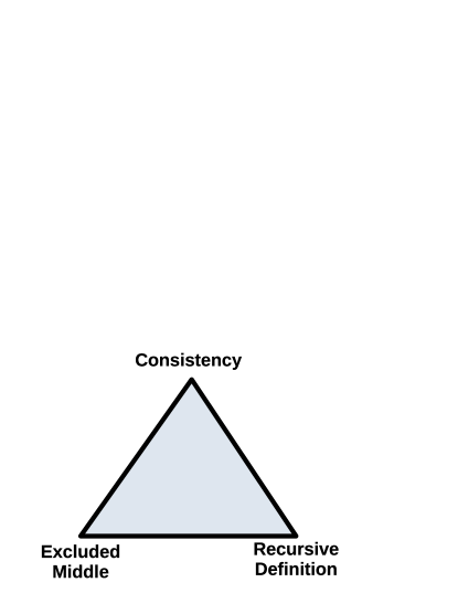
Figure 1: An impossibility triangle for logic. We may desire our logical reasoning to be (fully) consistent, to give us (unrestricted) use of the law of excludded middle or LEM, and to give us (unrestricted) recursive definition capability. It appears we must compromise at least one of these desires, however.

In the tradition of so-called “impossibility triangles,” Figure 1 shows one such triangle that appears to apply to systems of logic. Of three desirable properties we might wish for – namely (full) consistency, the (unrestricted) law of excluded middle or LEM, and (unrestricted) recursive definition, it appears we must compromise and accept a weakened version of at least one of these properties. Classical reasoning prioritizes full consistency and LEM while restricting recursive definitions, while in GD we will prioritize conssitency and recursive definition but weaken our LEM.

Beyond the immediate offering of unrestricted recursive definitions, the many indirect implications of GD’s alternative perspective on deduction rules and logical truth are interesting, in ways that this paper attempts to begin mapping, but on which it can admittedly only scratch the surface.

The cost of this flexibility manifests in GD’s deduction rules, many of which modify the rules of classical logic by incorporating typing requirements into their premises. For example, GD allows us to invoke proof by contradiction – assuming some proposition $p$ is false hypothetically in order to prove it true – only after we first prove that $p$ denotes a well-typed boolean value, i.e., that $p$ is in fact either true or false. GD’s inference rule for introducing logical implication $p\rightarrow q$ similarly requires us first to prove that $p$ is boolean, thereby avoiding Curry’s paradox, as we will see in Section 2.6.1.

Incorporating these typing requirements into GD’s basic deduction rules, fixed at the boundary between GD and whatever language or metalogic we use to reason about it, appears crucial in avoiding so-called revenge problems, where solving a pardox in one place just makes a more subtle but equally-insidious paradox appear elsewhere.

Satisfying GD’s typing requirements does impose a “reasoning cost” over the familiar rules of classical logic. In the common case, however, these typing proofs tend to be trivial and will likely be subject to future automation with appropriate tooling. As GD’s goal is to formulate a plausible working logic, the priority is to offer a reasonably complete set of familiar logical and mathematical tools in the new framework, ideally comprehensible not just to experts in mathematical logic or programming language theory, but also to non-experts. As a result, this formulation makes no attempt at minimalism. Many operators we introduce are definable in terms of others, and many deduction rules are derivable from combinations of others, as we note in places. The author thus offers apologies in advance to experts in logic to whom this style of formulation and exposition may feel unbearably verbose, tedious, and often redundant.

This working paper is a draft that is both preliminary and incomplete. In particular, what is presented here is only the first part of a much longer document, subsequent parts of which will be released in updates to this preprint as they reach a state of approximate readiness and readability. There may well be significant gaps or errors in parts already released, and rigorous formal analysis remains to be done. The author asks readers to take this current draft, whatever its state, as a preliminary basis for exploration, discussion, and further development, and not (yet) as a finished product.

2 Propositional deduction in GD

Mirroring the traditional starting point for defining logic, we first introduce the basic propositional connectives in GD for logical negation ($\neg$), conjunction ($\land$), disjunction ($\lor$), implication ($\rightarrow$), and biconditional ($\leftrightarrow$). In the process, we introduce GD’s approach to typing, judgments and deduction.

Classical logic in general, and the law of the excluded middle (LEM) especially, presuppose that any syntactically-valid proposition has an associated truth value of either true or false. Even many-valued logics such as Kleene’s 3-valued logic typically retain the underlying premise that every proposition has some particular truth value, while expanding the range of “choices” for what that value might be.

GD starts by rejecting this presumption, treating it as the “original sin” of classical logic. In GD, a proposition by default has no value of any type. In fact, GD does not even syntactically distinguish logical propositions from terms denoting mathematical objects such as integers or sets. Any syntactic expression is merely an untyped term – until that term is logically proven to represent a value (of some type) through a “grounded” deduction process. That is, until and unless we have proven that a term denotes a value of some type, we refuse to ascribe any value or type to that term – not even a “third value” in the usual sense for 3-valued logics.

2.1 Boolean truth values (bool)

We will typically use the letters $a,b,c$ to represent terms in some abstract or concrete syntax. A term might in principle represent any type of value (number, set, etc.). A term might just as well represent no definable value at all, such as the “result” of a paradox or computation that never terminates, and thus never actually yields any value.

For the present, we do not care exactly what kinds of values a term $a$ might represent (if indeed it has a value at all). Instead, we care only that there is at least one such expressible value that we will call “a true value.” We also assume there is at least one expressible value that we will call “a false value.” A value that falls into either of these categories we will call a boolean truth value, or simply a bool for short.

We require that no value be both true and false, but we otherwise set no expectations on what these truth values actually are. We are also agnostic to how many distinct true values and how many false values might exist. There might be only one unique true value named true, and one distinguished false value named false, as in many strongly-typed programming languages. Alternatively, truth values might be single-digit binary integers, with 1 as the unique true value, 0 as the unique false value, and all other numbers not denoting truth values. We might even take all integers to be truth values, with 0 as the only false value and all other integers representing true, as in many weakly-typed languages such as C. Which particular values might represent true and false will not concern us here; we assume merely that such values exist.

Consistent with these assumptions, we might consider the names true, false, and bool to denote types of values. From this perspective, the types true and false are each subtypes of type bool. That is, any value of type true is also of type bool, but the converse does not hold. If we view truth values as types, however, we do so only in the “weakly-typed” sense that we assume that concrete values of these types are reliably recognizable via some computation. We do not require all terms to have well-formed types in some type system, or expect that all all terms terms denoting truth values to be syntactically distinguishable (e.g., as “propositions”) from terms denoting other non-truth values. A term is just a term, which might but need not denote a truth value.

2.2 Type judgments and inference rules

If $a$ is an arbitrary term, then ‘$a\textsf{ true}$’ expresses a type judgment or claim that term $a$ denotes a true value (any true value if there is more than one). Similarly, ‘$a\textsf{ false}$’ is a type judgment that $a$ denotes a false value. Finally, ‘$a\textsf{ bool}$’ is a type judgment that $a$ denotes any boolean truth value, that is, either a true value or a false value.

We will next use judgments to form inference rules in traditional natural deduction style. To illustrate, we first introduce the following two basic inference rules:

$$\cfrac{a\textsf{ true}}{a\textsf{ bool}}\IfStrEq{boolI1}{}{}{\ \mathit{boolI1}}\qquad\cfrac{a\textsf{ false}}{a\textsf{ bool}}\IfStrEq{boolI2}{}{}{\ \mathit{boolI2}}$$

Inference rules indicate any premises above the line, a conclusion below the line, and optionally a label for the inference rule to the right. The first rule above, $\mathit{boolI1}$, states that if it is known (i.e., already proven) that term $a$ denotes a true value, then we may safely infer the weaker conclusion that $a$ denotes some boolean truth value (i.e., that $a$ is either true or false). The second rule similarly allows us to infer the weaker type judgment ‘$a\textsf{ bool}$’ if we have already proven the type judgment ‘$a\textsf{ false}$’.

The next inference rule illustrates multiple premises and hypothetical inference:

$$\cfrac{a\textsf{ bool}\qquad\begin{matrix}a\textsf{ true}\\ \vdots\\ c\textsf{ true}\end{matrix}\qquad\begin{matrix}a\textsf{ false}\\ \vdots\\ c\textsf{ true}\end{matrix}}{c\textsf{ true}}\IfStrEq{boolE}{}{}{\ \mathit{boolE}}$$

This rule states that we can draw the conclusion ‘$c\textsf{ true}$’ provided we first satisfy three conditions stated by the premises. The first premise ‘$a\textsf{ bool}$’ states that term $a$ must first be known (i.e., already proven) to be boolean. Second, starting from a hypothetical assumption of ‘$a\textsf{ true}$’, we must be able to derive through some correct chain of reasoning the conclusion ‘$c\textsf{ true}$’. Finally, starting from the contrary hypothesis ‘$a\textsf{ false}$’, we must likewise be able to derive the same conclusion ‘$c\textsf{ true}$’.

We may consider the first two inference rules above, $\mathit{boolI1}$ and $\mathit{boolI2}$, to be introduction rules for boolean type judgments. These rules introduce a type judgment of the form ‘$a\textsf{ bool}$’ into the conclusion, provided we are reasoning forwards from premises towards conclusion. The last rule above, in contrast, is an elimination rule for boolean type judgments. That is, the $\mathit{boolE}$ rule effectively eliminates a type judgment of the form ‘$a\textsf{ bool}$’ from the premises, thereby making it possible to reason in terms of true and false judgments alone, within the other two hypothetical premises.

The three inference rules above will be the only ones we need in order to define the relationship between boolean, true, and false type judgments in GD.

2.2.1 Boolean case analysis

Provided that $a$ is known to denote a boolean truth value (we have proven ‘$a\textsf{ bool}$’), the elimination rule $\mathit{boolE}$ above allows us to perform case analysis on $a$. That is, we can prove the goal ‘$b\textsf{ true}$’ in one fashion in the case where $a$ happens to be true, while we might prove the same goal in a different fashion in the case where $a$ is false.

With this power of case analysis, for example, we can immediately derive one rule for proof by contradiction. By taking $c$ to be the same as $a$ in the $\mathit{boolE}$ rule above, the second premise of $\mathit{boolE}$ becomes trivial, and we get the following derived rule representing a particular special case of boolean case analysis:

$$\cfrac{a\textsf{ bool}\qquad\begin{matrix}a\textsf{ false}\\ \vdots\\ a\textsf{ true}\end{matrix}}{a\textsf{ true}}\IfStrEq{}{}{}{\ \mathit{}}$$

That is, if $a$ is already proven to be boolean, and if from the hypothetical assumption that $a$ is false we can prove the contrary judgment that $a$ is true, then we can deduce the non-hypothetical conclusion that $a$ must be unconditionally true.

2.2.2 Judgments as terms

We will normally use type judgments like ‘$a\textsf{ true}$’ or ‘$a\textsf{ bool}$’ in defining inference rules such as those above. In GD these judgments may also serve as ordinary terms, however, expressing the proposition that a term denotes a value of a particular type. Formalizing this principle, the following rules express this equivalence: first for the specific example of the bool type, then in general for any name $\tau$ denoting a type:

$$\cfrac{a\textsf{ bool}}{(a\textsf{ bool})\textsf{ true}}\IfStrEq{}{}{}{\ \mathit{}}\qquad\cfrac{(a\textsf{ bool})\textsf{ true}}{a\textsf{ bool}}\IfStrEq{}{}{}{\ \mathit{}}\qquad\cfrac{a\textsf{ $\tau$}}{(a\textsf{ $\tau$})\textsf{ true}}\IfStrEq{}{}{}{\ \mathit{}}\qquad\cfrac{(a\textsf{ $\tau$})\textsf{ true}}{a\textsf{ $\tau$}}\IfStrEq{}{}{}{\ \mathit{}}$$

2.3 Logical negation $\neg$

We next introduce the logical negation operator, ‘$\neg$’. Given any term $a$, we can construct a term ‘$\neg a$’ denoting the logical negation of $a$. The following inference rules define logical negation in terms of the true and false type judgments above:

$$\cfrac{a\textsf{ true}}{\neg a\textsf{ false}}\IfStrEq{\neg I1}{}{}{\ \mathit{\neg I1}}\qquad\cfrac{a\textsf{ false}}{\neg a\textsf{ true}}\IfStrEq{\neg I2}{}{}{\ \mathit{\neg I2}}\qquad\cfrac{\neg a\textsf{ false}}{a\textsf{ true}}\IfStrEq{\neg E1}{}{}{\ \mathit{\neg E1}}\qquad\cfrac{\neg a\textsf{ true}}{a\textsf{ false}}\IfStrEq{\neg E2}{}{}{\ \mathit{\neg E2}}$$

These rules take the form of introduction and elimination rules, respectively, for logical negation. The fact that we can express both true (‘$a\textsf{ true}$’) and false type judgments (‘$a\textsf{ false}$’), and not just the former, allows for a simpler formulation than the traditional introduction and elimination rules for logical negation in classical logic.

In the interest of more concise notation, we can combine the four inference rules above into the following two bidirectional or equivalence rules:

$${\displaystyle\mathinner{\mathchoice{\ooalign{\raisebox{0.75pt}{$\displaystyle\frac{a\textsf{ true}}{\phantom{\neg a\textsf{ false}}}$}\cr\raisebox{-0.75pt}{$\displaystyle\frac{\phantom{a\textsf{ true}}}{\neg a\textsf{ false}}$}\cr}}{\ooalign{\raisebox{0.75pt}{$\textstyle\frac{a\textsf{ true}}{\phantom{\neg a\textsf{ false}}}$}\cr\raisebox{-0.75pt}{$\textstyle\frac{\phantom{a\textsf{ true}}}{\neg a\textsf{ false}}$}\cr}}{\ooalign{\raisebox{0.75pt}{$\scriptstyle\frac{a\textsf{ true}}{\phantom{\neg a\textsf{ false}}}$}\cr\raisebox{-0.75pt}{$\scriptstyle\frac{\phantom{a\textsf{ true}}}{\neg a\textsf{ false}}$}\cr}}{\ooalign{\raisebox{0.75pt}{$\scriptscriptstyle\frac{a\textsf{ true}}{\phantom{\neg a\textsf{ false}}}$}\cr\raisebox{-0.75pt}{$\scriptscriptstyle\frac{\phantom{a\textsf{ true}}}{\neg a\textsf{ false}}$}\cr}}}}\IfStrEq{\neg IE1}{}{}{\ \mathit{\neg IE1}}\qquad{\displaystyle\mathinner{\mathchoice{\ooalign{\raisebox{0.75pt}{$\displaystyle\frac{a\textsf{ false}}{\phantom{\neg a\textsf{ true}}}$}\cr\raisebox{-0.75pt}{$\displaystyle\frac{\phantom{a\textsf{ false}}}{\neg a\textsf{ true}}$}\cr}}{\ooalign{\raisebox{0.75pt}{$\textstyle\frac{a\textsf{ false}}{\phantom{\neg a\textsf{ true}}}$}\cr\raisebox{-0.75pt}{$\textstyle\frac{\phantom{a\textsf{ false}}}{\neg a\textsf{ true}}$}\cr}}{\ooalign{\raisebox{0.75pt}{$\scriptstyle\frac{a\textsf{ false}}{\phantom{\neg a\textsf{ true}}}$}\cr\raisebox{-0.75pt}{$\scriptstyle\frac{\phantom{a\textsf{ false}}}{\neg a\textsf{ true}}$}\cr}}{\ooalign{\raisebox{0.75pt}{$\scriptscriptstyle\frac{a\textsf{ false}}{\phantom{\neg a\textsf{ true}}}$}\cr\raisebox{-0.75pt}{$\scriptscriptstyle\frac{\phantom{a\textsf{ false}}}{\neg a\textsf{ true}}$}\cr}}}}\IfStrEq{\neg IE2}{}{}{\ \mathit{\neg IE2}}$$

The double line indicates that the rule is bidirectional, representing both an introduction and a corresponding elimination rule at once. Reading the bidirectional rule “as usual” with premise above and conclusion below the double line, these rules serve as introduction rules. Flipping the bidirectional rule vertically, however – taking the judgment below the line as the premise and the judgment above the line as conclusion – we get the corresponding elimination rule. A bidirectional rule thus states in effect that the form of judgment above the line is logically equivalent to, and hence freely interchangeable with, the form of judgment below the line.

Using the above rules and boolean case analysis ($\mathit{boolE}$), we can derive a bidirectional typing rule stating that if term $a$ is a boolean then so is ‘$\neg a$’, and vice versa:

$${\displaystyle\mathinner{\mathchoice{\ooalign{\raisebox{0.75pt}{$\displaystyle\frac{a\textsf{ bool}}{\phantom{\neg a\textsf{ bool}}}$}\cr\raisebox{-0.75pt}{$\displaystyle\frac{\phantom{a\textsf{ bool}}}{\neg a\textsf{ bool}}$}\cr}}{\ooalign{\raisebox{0.75pt}{$\textstyle\frac{a\textsf{ bool}}{\phantom{\neg a\textsf{ bool}}}$}\cr\raisebox{-0.75pt}{$\textstyle\frac{\phantom{a\textsf{ bool}}}{\neg a\textsf{ bool}}$}\cr}}{\ooalign{\raisebox{0.75pt}{$\scriptstyle\frac{a\textsf{ bool}}{\phantom{\neg a\textsf{ bool}}}$}\cr\raisebox{-0.75pt}{$\scriptstyle\frac{\phantom{a\textsf{ bool}}}{\neg a\textsf{ bool}}$}\cr}}{\ooalign{\raisebox{0.75pt}{$\scriptscriptstyle\frac{a\textsf{ bool}}{\phantom{\neg a\textsf{ bool}}}$}\cr\raisebox{-0.75pt}{$\scriptscriptstyle\frac{\phantom{a\textsf{ bool}}}{\neg a\textsf{ bool}}$}\cr}}}}\IfStrEq{\neg TIE}{}{}{\ \mathit{\neg TIE}}$$

We can now derive rules for proof by contradiction in terms of logical negation, by using case analysis ($\mathit{boolE}$) and $\neg I$:

$$\cfrac{a\textsf{ bool}\qquad\begin{matrix}\neg a\textsf{ true}\\ \vdots\\ a\textsf{ true}\end{matrix}}{a\textsf{ true}}\IfStrEq{}{}{}{\ \mathit{}}\qquad\cfrac{a\textsf{ bool}\qquad\begin{matrix}a\textsf{ true}\\ \vdots\\ \neg a\textsf{ true}\end{matrix}}{\neg a\textsf{ true}}\IfStrEq{}{}{}{\ \mathit{}}$$

From these rules and boolean case analysis we can in turn derive the more traditional inference rules for negation introduction and elimination, respectively:

$$\cfrac{a\textsf{ bool}\qquad\begin{matrix}a\textsf{ true}\\ \vdots\\ b\textsf{ true}\end{matrix}}{\neg a\textsf{ true}}\IfStrEq{}{}{}{\ \mathit{}}\qquad\cfrac{\neg a\textsf{ true}\qquad a\textsf{ true}}{b\textsf{ true}}\IfStrEq{}{}{}{\ \mathit{}}$$

The first rule requires a chain of reasoning leading from the hypothetical judgment ‘$a\textsf{ true}$’ to a proof of an arbitrary term $b$ used only in this premise: i.e., a proof that if $a$ is true then anything is provable. Simply taking $b$ to be ‘$\neg a$’ converts this rule into the earlier one for ‘$\neg a\textsf{ true}$’.

The second rule similarly derives a proof of an arbitrary term $b$ from the contradictory premises of both $\neg a$ and $a$. We derive this rule by applying case analysis rule $\mathit{boolE}$, and using the contradictory assumptions $\neg a$ and $a$ to discharge the hypothetical premises in both cases.

Finally we derive the most concise of the standard rules for proof by contradiction, namely double-negation introduction and elimination, as a bidirectional rule:

$${\displaystyle\mathinner{\mathchoice{\ooalign{\raisebox{0.75pt}{$\displaystyle\frac{a\textsf{ true}}{\phantom{\neg\neg a\textsf{ true}}}$}\cr\raisebox{-0.75pt}{$\displaystyle\frac{\phantom{a\textsf{ true}}}{\neg\neg a\textsf{ true}}$}\cr}}{\ooalign{\raisebox{0.75pt}{$\textstyle\frac{a\textsf{ true}}{\phantom{\neg\neg a\textsf{ true}}}$}\cr\raisebox{-0.75pt}{$\textstyle\frac{\phantom{a\textsf{ true}}}{\neg\neg a\textsf{ true}}$}\cr}}{\ooalign{\raisebox{0.75pt}{$\scriptstyle\frac{a\textsf{ true}}{\phantom{\neg\neg a\textsf{ true}}}$}\cr\raisebox{-0.75pt}{$\scriptstyle\frac{\phantom{a\textsf{ true}}}{\neg\neg a\textsf{ true}}$}\cr}}{\ooalign{\raisebox{0.75pt}{$\scriptscriptstyle\frac{a\textsf{ true}}{\phantom{\neg\neg a\textsf{ true}}}$}\cr\raisebox{-0.75pt}{$\scriptscriptstyle\frac{\phantom{a\textsf{ true}}}{\neg\neg a\textsf{ true}}$}\cr}}}}\IfStrEq{\neg\neg IE}{}{}{\ \mathit{\neg\neg IE}}$$

This formulation needs no ‘$a\textsf{ bool}$’ premise because the typing rules above imply that $\neg\neg a$, $\neg a$, and $a$ are all boolean provided that any one of them is boolean. We can then derive this rule from those above by contradiction.

The fact that double-negation elimination holds in GD makes it immediately obvious that GD makes no attempt to be intuitionistic in the tradition initiated by L.E.J. Brouwer, which traditionally rejects this equivalence. This is one way in which GD may feel more familiar and accesible than intuitionistic logic to those accustomed to classical logic, despite the new typing requirements that GD introduces.

2.4 Definitions, self-reference, and paradox

We now introduce into GD the ability to express definitions, in the following form:

$$s\equiv d$$

This form specifically represents a constant definition, in which we assign an arbitrary but not-yet-used symbol, $s$, as a constant symbol to represent another arbitrary term $d$. We henceforth refer to term $d$ as the expansion of the constant symbol $s$. In essence, the definition establishes the logical equivalence of symbol $s$ with its expansion $d$, in that either may subsequently be substituted for the other in a term. We focus on constant definitions to keep things simpler for now, but will introduce parameterized non-constant definitions later in Section 3.7.

2.4.1 Using definitions

We explicitly represent the use of definitions in GD via the following inference rules:

$$\cfrac{s\equiv d\qquad{p}\langle{d}\rangle\textsf{ true}}{{p}\langle{s}\rangle\textsf{ true}}\IfStrEq{{\equiv}I}{}{}{\ \mathit{{\equiv}I}}\qquad\cfrac{s\equiv d\qquad{p}\langle{s}\rangle\textsf{ true}}{{p}\langle{d}\rangle\textsf{ true}}\IfStrEq{{\equiv}E}{}{}{\ \mathit{{\equiv}E}}$$

The notation ‘${p}\langle{\cdot}\rangle$’ in the above rules represents a syntactic template that can express substitutions for free variables. In particular, if $x$ denotes a variable, the notation ‘${p}\langle{x}\rangle$’ represents an otherwise-arbitrary term $p$ having exactly one free variable $x$. If $d$ is a term, the notation ‘${p}\langle{d}\rangle$’ represents same term $p$ after replacing all instances of the free variable $x$ with term $d$. The notation ‘${p}\langle{s}\rangle$’ similarly represents the same term $p$ after replacing all instances of the same free variable $x$ with the defined symbol $s$.

Since the free variable $x$ itself does not appear in the above rules, the template term $p$ containing $x$ serves only as a context in these rules indicating where an instance of the definition’s expansion $d$ is to be replaced with the defined symbol $s$ in the introduction rule $\mathit{{\equiv}I}$, or vice-versa within the elimination rule $\mathit{{\equiv}E}$.

The pair of inference rules above describing definitional substitution have a form that will be common in GD, so we will use shorthand notation that combines both rules into a single more concise conditional bidirectional rule as follows:

$$\cfrac{s\equiv d\qquad}{}{\displaystyle\mathinner{\mathchoice{\ooalign{\raisebox{0.75pt}{$\displaystyle\frac{{p}\langle{d}\rangle\textsf{ true}}{\phantom{{p}\langle{s}\rangle\textsf{ true}}}$}\cr\raisebox{-0.75pt}{$\displaystyle\frac{\phantom{{p}\langle{d}\rangle\textsf{ true}}}{{p}\langle{s}\rangle\textsf{ true}}$}\cr}}{\ooalign{\raisebox{0.75pt}{$\textstyle\frac{{p}\langle{d}\rangle\textsf{ true}}{\phantom{{p}\langle{s}\rangle\textsf{ true}}}$}\cr\raisebox{-0.75pt}{$\textstyle\frac{\phantom{{p}\langle{d}\rangle\textsf{ true}}}{{p}\langle{s}\rangle\textsf{ true}}$}\cr}}{\ooalign{\raisebox{0.75pt}{$\scriptstyle\frac{{p}\langle{d}\rangle\textsf{ true}}{\phantom{{p}\langle{s}\rangle\textsf{ true}}}$}\cr\raisebox{-0.75pt}{$\scriptstyle\frac{\phantom{{p}\langle{d}\rangle\textsf{ true}}}{{p}\langle{s}\rangle\textsf{ true}}$}\cr}}{\ooalign{\raisebox{0.75pt}{$\scriptscriptstyle\frac{{p}\langle{d}\rangle\textsf{ true}}{\phantom{{p}\langle{s}\rangle\textsf{ true}}}$}\cr\raisebox{-0.75pt}{$\scriptscriptstyle\frac{\phantom{{p}\langle{d}\rangle\textsf{ true}}}{{p}\langle{s}\rangle\textsf{ true}}$}\cr}}}}\IfStrEq{{\equiv}IE}{}{}{\ \mathit{{\equiv}IE}}$$

A rule of this form expresses essentially that provided the common premise above the single line on the left side has been satisfied (in this case that a definition ‘$s\equiv d$’ exists), the premise above and conclusion below the right-hand, double-lined part of the rule may be used in either direction as a logical equivalence. That is, provided there is a definition ‘$s\equiv d$’, we can replace ‘${p}\langle{d}\rangle\textsf{ true}$’ with ‘${p}\langle{s}\rangle\textsf{ true}$’ and vice versa.

2.4.2 First-class definitions versus metalogical abbreviations

The careful construction and use of definitions is ubiquitous and essential in the normal practice of working mathematics and theoretical computer science. Ironically, however, definitions per se are often entirely from the formal logics constructed and studied by logicians, such as classical first-order logic. This is because standard practice is to treat definitions merely as metalogical abbreviations or shorthand notations: i.e., textual substitutions, like macros in many programming languages, that we could in principle just expand in our heads before commencing the real work of logical reasoning.

For this “definitions as shorthand abbreviations” perspective to work, however, standard practice holds that definitions must be non-recursive. That is, the newly-defined symbol $s$ in a definition ‘$s\equiv d$’ must not appear in the expansion $d$. Instead, the new symbol $s$ must be used only after the definition is complete. This crucial restriction avoids numerous tricky issues including the paradoxes we will explore shortly, while also tremendously reducing the expressiveness and utility of definitions.

In GD, in contrast, we will treat definitions as “first-class citizens” of the logic, rather than only as metalogical abbreviations. That is, we will treat definitions like ‘$s\equiv d$’ as actual steps in a formal logical proof, just as definitions normally appear before and intermixed with theorems in a working mathematical paper or textbook.

Both definitions and the bidirectional inference rules we have used above have the same apparent effect, of establishing logical equivalences. We draw an important semantic difference between them, however. Like other inference rules, a bidirectional equivalence rule is a purely metalogical construct: a convention we use to describe and reason about GD in our informal metalogic of ordinary English supplemented with traditional mathematical notation and concepts. A definition, in contrast, is not just metalogical but a first-class citizen within the logic of GD. Although the definitional equivalence symbol ‘$\equiv$’ is not part of GD’s term syntax, this symbol is part of GD’s proof syntax, since definitions appear in GD proofs alongside ordinary deductions.

We maintain the standard requirement that a given symbol $s$ must be defined only once: a proof must have at most one definition with a given symbol $s$ on the left-hand side. Allowing a symbol to be redefined – e.g., to yield a true value by one definition and a false value by another – would of course yield immediate contradictions.

GD will recklessly tempt fate, however, by allowing definitions to be recursive or self-referential. Within a definition ‘$s\equiv d$’, the newly-defined symbol $s$ may also appear any number of times, without restriction, within the definition’s right-hand-side expansion $d$. We will shortly explore the effects of recursive definitions.

2.4.3 The Liar Paradox

Let us see how our recklessly self-referential logic fares against the venerable liar paradox, readily expressible in words as follows:

This statement is false.

If we suppose hypothetically that the above statement is true, then we must logically conclude that it is false, and vice versa. It is thus both true and false, a contradiction.

We can readily express the liar paradox in a definition of GD as follows:

$$L\equiv\neg L$$

If allowed, this definition would immediately doom classical logic, which assumes that every syntactically well-formed proposition such as $L$ must be either true or false. Applying classical proof by contradiction, for example, we hypothetically assume $L$ is true, then unwrap its definition once to yield $\neg L$, a contradiction. Since the hypothesis $L$ yielded the conclusion $\neg L$, it follows that $L$ must also be true non-hypothetically. But then $\neg L$ is also true non-hypothetically, and we can prove anything.

GD’s deduction rules above do not permit us proof by contradiction about just any syntactically well-formed term $a$, however. Instead, our proof by contradiction rules first require us to prove ‘$a\textsf{ bool}$’: i.e., that $a$ is a term that actually denotes a boolean value. Only then may we assume that $a$ must be either true or false and invoke any flavor of the law of the excluded middle or proof by contradiction.

In the case of the liar paradox statement $L$, we could prove ‘$L\textsf{ bool}$’ if we could find a way to prove that ‘$\neg L$’, ‘$\neg\neg L$’, or any other such variant denotes a boolean value. But we will have difficulty doing so, as we find no well-founded, non-circular grounds to support such a claim. In particular, in attempting to prove that $L$ is boolean, we run into the practical conundrum of first having to prove that $L$ is boolean. We can assign $L$ no truth value because it is ungrounded, to adopt Kripke’s terminology.

We will of course revisit the paradox question, multiple times, as we acquire more interesting and seemingly-dangerous logical toys to play with.

2.5 Logical conjunction $\land$ and disjunction $\lor$

We introduce conjunction terms of the form ‘$a\land b$’ with the classical deduction rules:

$$\cfrac{a\textsf{ true}\qquad b\textsf{ true}}{a\land b\textsf{ true}}\IfStrEq{\land I1}{}{}{\ \mathit{\land I1}}\qquad\cfrac{a\land b\textsf{ true}}{a\textsf{ true}}\IfStrEq{\land E1}{}{}{\ \mathit{\land E1}}\qquad\cfrac{a\land b\textsf{ true}}{b\textsf{ true}}\IfStrEq{\land E2}{}{}{\ \mathit{\land E2}}$$

The introduction rule $\mathit{\land I1}$ allows us to introduce logical conjunction into a conclusion of the form ‘$a\land b\textsf{ true}$’, contingent on the premises of ‘$a\textsf{ true}$’ and ‘$b\textsf{ true}$’ each already holding individually. The two elimination rules $\mathit{\land E1}$ and $\mathit{\land E2}$ weaken the premise ‘$a\land b\textsf{ true}$’ into a conclusion of ‘$a\textsf{ true}$’ or ‘$b\textsf{ true}$’ alone, respectively.

The above rules allow us to reason only about the true cases relating to judgments of the form ‘$a\land b\textsf{ true}$’. We will also need to reason about cases in which a logical conjunction is false, a purpose served by the following rules:

$$\cfrac{a\textsf{ false}}{a\land b\textsf{ false}}\IfStrEq{\land I2}{}{}{\ \mathit{\land I2}}\qquad\cfrac{b\textsf{ false}}{a\land b\textsf{ false}}\IfStrEq{\land I3}{}{}{\ \mathit{\land I3}}\qquad\cfrac{a\land b\textsf{ false}\qquad\begin{matrix}a\textsf{ false}\\ \vdots\\ c\textsf{ true}\\ \end{matrix}\qquad\begin{matrix}b\textsf{ false}\\ \vdots\\ c\textsf{ true}\\ \end{matrix}}{c\textsf{ true}}\IfStrEq{\land E3}{}{}{\ \mathit{\land E3}}$$

The false-case introduction rules $\mathit{\land I2}$ and $\mathit{\land I3}$ allow us to infer ‘$a\land b\textsf{ false}$’ given a proof of either ‘$a\textsf{ false}$’ or ‘$b\textsf{ false}$’. The false-case elimination rule $E3$ essentially performs case analysis on the premise ‘$a\land b\textsf{ false}$’ to be eliminated. Provided the conclusion ‘$c\textsf{ true}$’ may be inferred separately (and likely via different reasoning steps) from either of the hypotheses ‘$a\textsf{ false}$’ or ‘$b\textsf{ false}$’, the premise ‘$a\land b\textsf{ false}$’ ensures the conclusion ‘$c\textsf{ true}$’ regardless of which of $a$ and/or $b$ are actually false.

The following rules similarly address the true and false cases of logical disjunction:

$$\cfrac{a\textsf{ true}}{a\lor b\textsf{ true}}\IfStrEq{\lor I1}{}{}{\ \mathit{\lor I1}}\qquad\cfrac{b\textsf{ true}}{a\lor b\textsf{ true}}\IfStrEq{\lor I2}{}{}{\ \mathit{\lor I2}}\qquad\cfrac{a\lor b\textsf{ true}\qquad\begin{matrix}a\textsf{ true}\\ \vdots\\ c\textsf{ true}\\ \end{matrix}\qquad\begin{matrix}b\textsf{ true}\\ \vdots\\ c\textsf{ true}\\ \end{matrix}}{c\textsf{ true}}\IfStrEq{\lor E1}{}{}{\ \mathit{\lor E1}}$$

$$\cfrac{a\textsf{ false}\qquad b\textsf{ false}}{a\lor b\textsf{ false}}\IfStrEq{\lor I3}{}{}{\ \mathit{\lor I3}}\qquad\cfrac{a\lor b\textsf{ false}}{a\textsf{ false}}\IfStrEq{\lor E2}{}{}{\ \mathit{\lor E2}}\qquad\cfrac{a\lor b\textsf{ false}}{b\textsf{ false}}\IfStrEq{\lor E3}{}{}{\ \mathit{\lor E3}}$$

The introduction rules $\mathit{\lor I1}$ and $\mathit{\lor I2}$ introduce ‘$a\lor b\textsf{ true}$’ given only an individual proof of either ‘$a\textsf{ true}$’ or ‘$b\textsf{ true}$’, respectively. The elimination rule essentially performs disjunctive case analysis. Provided the conclusion ‘$c\textsf{ true}$’ may be proven separately from either of the hypotheses ‘$a\textsf{ true}$’ or ‘$b\textsf{ true}$’, the disjunction in the premise ensures the conclusion regardless of which of $a$ and/or $b$ are in fact true. Similarly, the corresponding false-case rules naturally mirror the true-case rules for conjunction.

Just as in classical logic, conjunction and disjunction in GD are duals of each other: we can obtain either operator’s rules by taking those of the other and swapping true with false and swapping ‘$\land$’ with ‘$\lor$’. As a result, De Morgan’s laws work in GD just as in classical logic, as we express in the following bidirectional equivalence rules:

$${\displaystyle\mathinner{\mathchoice{\ooalign{\raisebox{0.75pt}{$\displaystyle\frac{\neg(\neg p\lor\neg q)}{\phantom{p\land q}}$}\cr\raisebox{-0.75pt}{$\displaystyle\frac{\phantom{\neg(\neg p\lor\neg q)}}{p\land q}$}\cr}}{\ooalign{\raisebox{0.75pt}{$\textstyle\frac{\neg(\neg p\lor\neg q)}{\phantom{p\land q}}$}\cr\raisebox{-0.75pt}{$\textstyle\frac{\phantom{\neg(\neg p\lor\neg q)}}{p\land q}$}\cr}}{\ooalign{\raisebox{0.75pt}{$\scriptstyle\frac{\neg(\neg p\lor\neg q)}{\phantom{p\land q}}$}\cr\raisebox{-0.75pt}{$\scriptstyle\frac{\phantom{\neg(\neg p\lor\neg q)}}{p\land q}$}\cr}}{\ooalign{\raisebox{0.75pt}{$\scriptscriptstyle\frac{\neg(\neg p\lor\neg q)}{\phantom{p\land q}}$}\cr\raisebox{-0.75pt}{$\scriptscriptstyle\frac{\phantom{\neg(\neg p\lor\neg q)}}{p\land q}$}\cr}}}}\IfStrEq{\land IE}{}{}{\ \mathit{\land IE}}\qquad{\displaystyle\mathinner{\mathchoice{\ooalign{\raisebox{0.75pt}{$\displaystyle\frac{\neg(\neg p\land\neg q)}{\phantom{p\lor q}}$}\cr\raisebox{-0.75pt}{$\displaystyle\frac{\phantom{\neg(\neg p\land\neg q)}}{p\lor q}$}\cr}}{\ooalign{\raisebox{0.75pt}{$\textstyle\frac{\neg(\neg p\land\neg q)}{\phantom{p\lor q}}$}\cr\raisebox{-0.75pt}{$\textstyle\frac{\phantom{\neg(\neg p\land\neg q)}}{p\lor q}$}\cr}}{\ooalign{\raisebox{0.75pt}{$\scriptstyle\frac{\neg(\neg p\land\neg q)}{\phantom{p\lor q}}$}\cr\raisebox{-0.75pt}{$\scriptstyle\frac{\phantom{\neg(\neg p\land\neg q)}}{p\lor q}$}\cr}}{\ooalign{\raisebox{0.75pt}{$\scriptscriptstyle\frac{\neg(\neg p\land\neg q)}{\phantom{p\lor q}}$}\cr\raisebox{-0.75pt}{$\scriptscriptstyle\frac{\phantom{\neg(\neg p\land\neg q)}}{p\lor q}$}\cr}}}}\IfStrEq{\lor IE}{}{}{\ \mathit{\lor IE}}$$

The fact that De Morgan’s laws continue to hold in GD as with classical logic may make GD feel slightly more familiar and accessible to some, despite the new typing requirements that many other inference rules impose in GD.

2.5.1 Typing rules for conjunction and disjunction

From the above rules we can finally derive the following straightforward typing rules for conjunction and disjunction:

$$\cfrac{a\textsf{ bool}\qquad b\textsf{ bool}}{a\land b\textsf{ bool}}\IfStrEq{\land TI}{}{}{\ \mathit{\land TI}}\qquad\cfrac{a\textsf{ bool}\qquad b\textsf{ bool}}{a\lor b\textsf{ bool}}\IfStrEq{\lor TI}{}{}{\ \mathit{\lor TI}}$$

Recall that logical negation in GD has a typing elimination rule $\mathit{\neg TE}$ that works in the reverse direction, allowing us to deduce ‘$a\textsf{ bool}$’ from ‘$\neg a\textsf{ bool}$’. Reverse-direction type deduction is not so simple for conjunction or disjunction, since the result may be boolean even if only one of the inputs is boolean. Nevertheless, we can derive the following reverse typing rules, reflecting the fact that at least one of the inputs to a conjunction or disjunction must be boolean in order to for the result to be boolean:

$$\cfrac{a\land b\textsf{ bool}\qquad\begin{matrix}a\textsf{ bool}\\ \vdots\\ c\textsf{ true}\\ \end{matrix}\qquad\begin{matrix}b\textsf{ bool}\\ \vdots\\ c\textsf{ true}\\ \end{matrix}}{c\textsf{ true}}\IfStrEq{\land TE}{}{}{\ \mathit{\land TE}}\qquad\cfrac{a\lor b\textsf{ bool}\qquad\begin{matrix}a\textsf{ bool}\\ \vdots\\ c\textsf{ true}\\ \end{matrix}\qquad\begin{matrix}b\textsf{ bool}\\ \vdots\\ c\textsf{ true}\\ \end{matrix}}{c\textsf{ true}}\IfStrEq{\lor TE}{}{}{\ \mathit{\lor TE}}$$

Now that we have logical disjunction, we might consider the booleanness of a term in terms of logical disjunction and negation. A term is boolean whenever its value is either true or false: that is, we may treat ‘$a\textsf{ bool}$’ as equivalent to ‘$a\lor\neg a\textsf{ true}$’:

$${\displaystyle\mathinner{\mathchoice{\ooalign{\raisebox{0.75pt}{$\displaystyle\frac{p\lor\neg p}{\phantom{p\textsf{ bool}}}$}\cr\raisebox{-0.75pt}{$\displaystyle\frac{\phantom{p\lor\neg p}}{p\textsf{ bool}}$}\cr}}{\ooalign{\raisebox{0.75pt}{$\textstyle\frac{p\lor\neg p}{\phantom{p\textsf{ bool}}}$}\cr\raisebox{-0.75pt}{$\textstyle\frac{\phantom{p\lor\neg p}}{p\textsf{ bool}}$}\cr}}{\ooalign{\raisebox{0.75pt}{$\scriptstyle\frac{p\lor\neg p}{\phantom{p\textsf{ bool}}}$}\cr\raisebox{-0.75pt}{$\scriptstyle\frac{\phantom{p\lor\neg p}}{p\textsf{ bool}}$}\cr}}{\ooalign{\raisebox{0.75pt}{$\scriptscriptstyle\frac{p\lor\neg p}{\phantom{p\textsf{ bool}}}$}\cr\raisebox{-0.75pt}{$\scriptscriptstyle\frac{\phantom{p\lor\neg p}}{p\textsf{ bool}}$}\cr}}}}\IfStrEq{boolIE}{}{}{\ \mathit{boolIE}}$$

2.5.2 Paradoxes revisited

With conjunction and disjunction, we can construct slightly more subtle and interesting paradoxes (and non-paradoxes). Consider the following statements intuitively, for example:

$S_{1}$: Snow is white.

$S_{2}$: Either statement $S_{1}$ or statement $S_{2}$ is true.

$S_{3}$: Statements $S_{2}$ and $S_{3}$ are both true.

Supposing $t$ is any true term, we can define these sentences in GD as follows:

$S_{1}\equiv\textsf{true}$

$S_{2}\equiv S_{1}\lor S_{2}$

$S_{3}\equiv S_{2}\land S_{3}$

Statement $S_{1}$ is trivially true, and only one operand of a disjunction need be true for the disjunction to be true. Therefore, the truth of statement $S_{1}$ makes statement $S_{2}$ likewise true, despite $S_{2}$’s self-reference in its second operand.

Statement $S_{3}$, however, we find ourselves unable to prove either true or false in GD. Because $S_{2}$ is true, $S_{3}$ effectively depends on its own value. We will not be able to invoke proof by contradiction on $S_{3}$ without first proving it boolean, and any such attempt will encounter the fact that $S_{3}$ must first have already been proven boolean.

$S_{3}$ is an example of a statement Kripke would classify as ungrounded but non-paradoxical: GD does not give it a truth value because of its circular dependency, but it could be “forced” to true (e.g., by axiom) without causing a logical inconsistency.

If $S_{2}$ happened to be false, of course, then it would be trivial to prove $S_{3}$ false.

2.6 Logical implication $\rightarrow$ and biconditional $\leftrightarrow$

Logical implication in GD exhibits the same equivalence as in classical logic, which we express in the following bidirectional inference rule:

$${\displaystyle\mathinner{\mathchoice{\ooalign{\raisebox{0.75pt}{$\displaystyle\frac{\neg p\lor q}{\phantom{p\rightarrow q}}$}\cr\raisebox{-0.75pt}{$\displaystyle\frac{\phantom{\neg p\lor q}}{p\rightarrow q}$}\cr}}{\ooalign{\raisebox{0.75pt}{$\textstyle\frac{\neg p\lor q}{\phantom{p\rightarrow q}}$}\cr\raisebox{-0.75pt}{$\textstyle\frac{\phantom{\neg p\lor q}}{p\rightarrow q}$}\cr}}{\ooalign{\raisebox{0.75pt}{$\scriptstyle\frac{\neg p\lor q}{\phantom{p\rightarrow q}}$}\cr\raisebox{-0.75pt}{$\scriptstyle\frac{\phantom{\neg p\lor q}}{p\rightarrow q}$}\cr}}{\ooalign{\raisebox{0.75pt}{$\scriptscriptstyle\frac{\neg p\lor q}{\phantom{p\rightarrow q}}$}\cr\raisebox{-0.75pt}{$\scriptscriptstyle\frac{\phantom{\neg p\lor q}}{p\rightarrow q}$}\cr}}}}\IfStrEq{{\rightarrow}IE}{}{}{\ \mathit{{\rightarrow}IE}}$$

Just as in classical logic, $a$ implies $b$ precisely when either $a$ is false or $b$ is true.

We can then derive introduction and elimination rules for implication, mostly classical except the introduction rule requires that the antecedent be proven to be boolean:

$$\cfrac{a\textsf{ bool}\qquad\begin{matrix}a\textsf{ true}\\ \vdots\\ b\textsf{ true}\\ \end{matrix}}{a\rightarrow b\textsf{ true}}\IfStrEq{{\rightarrow}I}{}{}{\ \mathit{{\rightarrow}I}}\qquad\cfrac{a\rightarrow b\textsf{ true}\qquad a\textsf{ true}}{b\textsf{ true}}\IfStrEq{{\rightarrow}E}{}{}{\ \mathit{{\rightarrow}E}}$$

The $\mathit{{\rightarrow}E}$ rule is identical to the classical modus ponens rule.

We can similarly express the logical biconditional or “if and only if” in GD via the same bidirectional equivalence that applies in classical logic:

$${\displaystyle\mathinner{\mathchoice{\ooalign{\raisebox{0.75pt}{$\displaystyle\frac{(p\rightarrow q)\land(q\rightarrow p)}{\phantom{p\leftrightarrow q}}$}\cr\raisebox{-0.75pt}{$\displaystyle\frac{\phantom{(p\rightarrow q)\land(q\rightarrow p)}}{p\leftrightarrow q}$}\cr}}{\ooalign{\raisebox{0.75pt}{$\textstyle\frac{(p\rightarrow q)\land(q\rightarrow p)}{\phantom{p\leftrightarrow q}}$}\cr\raisebox{-0.75pt}{$\textstyle\frac{\phantom{(p\rightarrow q)\land(q\rightarrow p)}}{p\leftrightarrow q}$}\cr}}{\ooalign{\raisebox{0.75pt}{$\scriptstyle\frac{(p\rightarrow q)\land(q\rightarrow p)}{\phantom{p\leftrightarrow q}}$}\cr\raisebox{-0.75pt}{$\scriptstyle\frac{\phantom{(p\rightarrow q)\land(q\rightarrow p)}}{p\leftrightarrow q}$}\cr}}{\ooalign{\raisebox{0.75pt}{$\scriptscriptstyle\frac{(p\rightarrow q)\land(q\rightarrow p)}{\phantom{p\leftrightarrow q}}$}\cr\raisebox{-0.75pt}{$\scriptscriptstyle\frac{\phantom{(p\rightarrow q)\land(q\rightarrow p)}}{p\leftrightarrow q}$}\cr}}}}\IfStrEq{{\leftrightarrow}IE}{}{}{\ \mathit{{\leftrightarrow}IE}}$$

Unlike implication, the biconditional introduction rule we derive includes premises demanding that we first prove both terms in question to be boolean:

$$\cfrac{a\textsf{ bool}\qquad b\textsf{ bool}\qquad\begin{matrix}a\textsf{ true}\\ \vdots\\ b\textsf{ true}\\ \end{matrix}\qquad\begin{matrix}b\textsf{ true}\\ \vdots\\ a\textsf{ true}\\ \end{matrix}}{a\leftrightarrow b\textsf{ true}}\IfStrEq{{\leftrightarrow}I}{}{}{\ \mathit{{\leftrightarrow}I}}$$

Two derived elimination rules, one for each direction, work as in classical logic:

$$\cfrac{a\leftrightarrow b\textsf{ true}\qquad a\textsf{ true}}{b\textsf{ true}}\IfStrEq{{\leftrightarrow}E1}{}{}{\ \mathit{{\leftrightarrow}E1}}\qquad\cfrac{a\leftrightarrow b\textsf{ true}\qquad b\textsf{ true}}{a\textsf{ true}}\IfStrEq{{\leftrightarrow}E2}{}{}{\ \mathit{{\leftrightarrow}E2}}$$

As we did earlier with definitions in Section 2.4.1, we can combine the two rules above into a single, more concise, conditional bidirectional inference rule:

$$\cfrac{a\leftrightarrow b\textsf{ true}\qquad}{}{\displaystyle\mathinner{\mathchoice{\ooalign{\raisebox{0.75pt}{$\displaystyle\frac{a\textsf{ true}}{\phantom{b\textsf{ true}}}$}\cr\raisebox{-0.75pt}{$\displaystyle\frac{\phantom{a\textsf{ true}}}{b\textsf{ true}}$}\cr}}{\ooalign{\raisebox{0.75pt}{$\textstyle\frac{a\textsf{ true}}{\phantom{b\textsf{ true}}}$}\cr\raisebox{-0.75pt}{$\textstyle\frac{\phantom{a\textsf{ true}}}{b\textsf{ true}}$}\cr}}{\ooalign{\raisebox{0.75pt}{$\scriptstyle\frac{a\textsf{ true}}{\phantom{b\textsf{ true}}}$}\cr\raisebox{-0.75pt}{$\scriptstyle\frac{\phantom{a\textsf{ true}}}{b\textsf{ true}}$}\cr}}{\ooalign{\raisebox{0.75pt}{$\scriptscriptstyle\frac{a\textsf{ true}}{\phantom{b\textsf{ true}}}$}\cr\raisebox{-0.75pt}{$\scriptscriptstyle\frac{\phantom{a\textsf{ true}}}{b\textsf{ true}}$}\cr}}}}\IfStrEq{{\leftrightarrow}E}{}{}{\ \mathit{{\leftrightarrow}E}}$$

From the above we can derive inference rules getting from a biconditional “back” to a logical implication in either direction:

$$\cfrac{a\leftrightarrow b\textsf{ true}}{a\rightarrow b\textsf{ true}}\IfStrEq{{\leftrightarrow}E3}{}{}{\ \mathit{{\leftrightarrow}E3}}\qquad\cfrac{a\leftrightarrow b\textsf{ true}}{b\rightarrow a\textsf{ true}}\IfStrEq{{\leftrightarrow}E4}{}{}{\ \mathit{{\leftrightarrow}E4}}$$

Finally, through boolean case analysis we can derive the following type-elimination rules that apply to the biconditional (but importantly, not to logical implication in GD). In essence, a biconditional in GD yields a boolean truth value not only when, but only when, both of its arguments are boolean:

$$\cfrac{a\leftrightarrow b\textsf{ bool}}{a\textsf{ bool}}\IfStrEq{{\leftrightarrow}TE1}{}{}{\ \mathit{{\leftrightarrow}TE1}}\qquad\cfrac{a\leftrightarrow b\textsf{ bool}}{b\textsf{ bool}}\IfStrEq{{\leftrightarrow}TE2}{}{}{\ \mathit{{\leftrightarrow}TE2}}$$

In general, we now have the machinery necessary to represent, and prove, any statement in classical propositional logic – provided, of course, that the constituent terms are first proven to be boolean as might be necessary.

2.6.1 Curry’s paradox

Another interesting paradox to examine is Curry’s paradox, which we may express informally as follows:

If this statement is true, then pigs fly.

Curry’s paradox is interesting in particular because it relies only on logical implication, and not on the law of excluded middle. Curry’s paradox therefore compromises even intuitionistic logics, if they were to admit self-referential definitions such as this.

We can express Curry’s paradox via a perfectly legal definition in GD, however:

$$C\equiv C\rightarrow P$$

With the traditional natural deduction rule for implication, without first proving anything else about $C$, we can hypothetically assume $C$ and attempt to derive arbitrary predicate $P$. Since $C\equiv C\rightarrow P$, this derivation follows trivially via modus ponens. But then we find that $C\rightarrow P$ is true non-hypothetically, that $C$ is likewise true by its definition, and hence (again by modus ponens) the truth of $P$, i.e., pigs fly.

In GD, however, the introduction rule for ‘$a\rightarrow b\textsf{ true}$’ carries an obligation first to prove ‘$a\textsf{ bool}$’. We will have trouble proving this for Curry’s statement $C$, however, since $C$’s implication depends on its own antecedent and we find no grounded basis to assign any truth value to it. As with the Liar paradox expressed in GD, we find ourselves first having to prove ‘$C\textsf{ bool}$’ in order to apply the $\mathit{{\rightarrow}I}$ rule in order to prove ‘$C\textsf{ bool}$’ (or in general to prove anything about $C$). Thus, GD appears to survive self-referential paradoxes that even intuitionistic logics do not.

3 Predicate logic: reasoning about objects

Moving beyond logical propositions, we now wish to reason logically about mathematical objects other than truth values: e.g., numbers, sets, functions, etc. We will thus wish to have the usual predicate-logic quantifiers, for all ($\forall$) and there exists ($\exists$).

3.1 Domain of discourse and object judgments

But what will be our domain of discourse – the varieties of mathematical objects that we quantify over? In the same spirit of our earlier agnosticism about which term values represent “true” or “false” values and how many of each there are, we likewise remain agnostic for now about precisely what kinds of objects we may quantify over in GD. We intentionally leave this question to be answered later, separately, in some specialization or application of the principles of GD that we cover here. In software engineering terms, we for now leave the domain of discourse as an open “configuration parameter” to our predicate logic.

Instead of settling on any particular domain of discourse, we merely introduce a new form of typing judgment for use in our inference rules:

$$a\textsf{ obj}$$

This judgment essentially states: “The term $a$ denotes an object in the domain of discourse to which the logical quantifiers apply.”

3.2 Universal quantification

Given this new form of type judgment, we define natural deduction rules for the universal quantifier $\forall$ as follows:

$$\cfrac{\begin{matrix}x\textsf{ obj}\\ \vdots\\ {p}\langle{x,\dots}\rangle\textsf{ true}\\ \end{matrix}}{\forall{x}\ {{p}\langle{x,\dots}\rangle\textsf{ true}}}\IfStrEq{\forall I1}{}{}{\ \mathit{\forall I1}}\qquad\cfrac{\forall{x}\ {{p}\langle{x,\dots}\rangle\textsf{ true}}\qquad a\textsf{ obj}}{{p}\langle{a,\dots}\rangle\textsf{ true}}\IfStrEq{\forall E1}{}{}{\ \mathit{\forall E1}}$$

The notation ‘${p}\langle{x,\dots}\rangle$’ represents a syntactic template as discussed earlier in Section 2.4.1, except in this case the ellipsis ‘$\dots$’ indicates that the template term $p$ may also contain other free variables in addition to $x$. As before, the notation ‘${p}\langle{a,\dots}\rangle$’ appearing in the $\forall E1$ rule represents the template term $p$ with another term $a$ substituted for the variable $x$ while avoiding variable capture.

The premise of the introduction rule $\mathit{\forall I1}$ posits a particular unspecified but quantifiable object denoted by some variable $x$, and demands a proof that a predicate term ${p}\langle{x,\dots}\rangle$ is true of $x$. This proof must thus be carried out without any knowledge of which particular quantifiable object the variable $x$ actually represents. Provided such a proof can be deduced about the unknown hypothetical object $x$, the introduction rule concludes that term ${p}\langle{x,\dots}\rangle$ holds true for all quantifiable objects $x$.

The elimination rule $\mathit{\forall E1}$ demands that some universally quantified term $\forall{x}\ {{p}\langle{x,\dots}\rangle}$ be true, and also that some arbitrary term $a$ of interest is already proven to denote a quantifiable object. Under these premises, we reason that the term ${p}\langle{a,\dots}\rangle$, where object term $a$ has been substituted for free variable $x$, must be true as a special case.

The new second premise ‘$a\textsf{ obj}$’ in the elimination rule $\mathit{\forall E1}$ represents the main difference between universal quantification in GD versus classical first-order logic. Classical first-order logic assumes that terms representing quantifiable objects are kept syntactically separate from logical formulas, and hence that any term that can be substituted for a variable $x$ in a quantifier is necessarily a quantifiable object. Because GD takes it as given that terms might denote anything (truth values, quantifiable objects, non-quantifiable objects) or nothing (paradoxical statements, non-terminating computations), it becomes essential to demand proof that $a$ in fact denotes a quantifiable object before we safely conclude that a universally-quantified truth applies to $a$.

As before in propositional logic, we also need to reason about the false case of universal quantification, i.e., where there is a counterexample to the quantified predicate. The following false-case inference rules serve this purpose:

$$\cfrac{a\textsf{ obj}\qquad{p}\langle{a,\dots}\rangle\textsf{ false}}{\forall{x}\ {{p}\langle{x,\dots}\rangle\textsf{ false}}}\IfStrEq{\forall I2}{}{}{\ \mathit{\forall I2}}\qquad\cfrac{\forall{x}\ {{p}\langle{x,\dots}\rangle\textsf{ false}}\qquad\begin{matrix}\underbrace{x\textsf{ obj}\qquad{p}\langle{x,\dots}\rangle\textsf{ false}}\\ \vdots\\ q\textsf{ true}\\ \end{matrix}}{q\textsf{ true}}\IfStrEq{\forall E2}{}{}{\ \mathit{\forall E2}}$$

The false-case introduction rule $\mathit{\forall I2}$ demands that some arbitrary term $a$ be known to denote a quantifiable object, and that some predicate term ${p}\langle{x,\dots}\rangle$ with a free variable $x$ be provably false when $a$ is substituted for $x$. Since this object $a$ serves as a counterexample demonstrating that ${p}\langle{x,\dots}\rangle$ is not true for all quantifiable objects $x$, we then conclude that the universally quantified predicate $\forall{x}\ {{p}\langle{x,\dots}\rangle}$ is false.

The false-case elimination rule $\mathit{\forall E2}$ allows us to make use of the knowledge that a universally quantified statement is false and thus has a counterexample. The $\mathit{\forall E2}$ rule takes as premises a universally-quantified predicate known to be false, together with a hypothetical line of reasoning from a variable $x$ denoting an arbitrary quantifiable object about which predicate ${p}\langle{x,\dots}\rangle$ is false, and concluding that term $q$ is true assuming these hypotheses. Upon satisfying these premises, the rule allows us to conclude that $q$ is true unconditionally (non-hypothetically). The conclusion term $q$ may not refer to the temporary variable $x$ used in the second hypothetical premise.

Apart from the incorporation of object typing requirements, both of these false-case rules operate similarly to the standard natural deduction rules for existential quantifiers in classical first-order logic. This should not be a surprise, in that their goal is to reason about the existence of a counterexample that falsifies a universally-quantified predicate.

3.3 Existential quantification

The following rules define existential quantification in GD:

$$\cfrac{a\textsf{ obj}\qquad{p}\langle{a,\dots}\rangle\textsf{ true}}{\exists{x}\ {{p}\langle{x,\dots}\rangle}\textsf{ true}}\IfStrEq{\exists I1}{}{}{\ \mathit{\exists I1}}\qquad\cfrac{\exists{x}\ {{p}\langle{x,\dots}\rangle}\textsf{ true}\qquad\begin{matrix}\underbrace{x\textsf{ obj}\qquad{p}\langle{x,\dots}\rangle\textsf{ true}}\\ \vdots\\ q\textsf{ true}\\ \end{matrix}}{q\textsf{ true}}\IfStrEq{\exists E1}{}{}{\ \mathit{\exists E1}}$$

$$\cfrac{\begin{matrix}x\textsf{ obj}\\ \vdots\\ {p}\langle{x,\dots}\rangle\textsf{ false}\\ \end{matrix}}{\exists{x}\ {{p}\langle{x,\dots}\rangle}\textsf{ false}}\IfStrEq{\exists I2}{}{}{\ \mathit{\exists I2}}\qquad\cfrac{\exists{x}\ {{p}\langle{x,\dots}\rangle}\textsf{ false}\qquad a\textsf{ obj}}{{p}\langle{a,\dots}\rangle\textsf{ false}}\IfStrEq{\exists E2}{}{}{\ \mathit{\exists E2}}$$

Just as in classical logic, universal and existential quantification are duals of each other in GD. That is, we may obtain the rules for either from those of the other simply by swapping true with false and simultaneously swapping ‘$\forall$’ with ‘$\exists$’. As a result, the classical equivalences between universal and existential quantification continue to hold in GD, as expressed in the following bidirectional inference rules:

$${\displaystyle\mathinner{\mathchoice{\ooalign{\raisebox{0.75pt}{$\displaystyle\frac{\neg\exists{x}\ {{\neg p}\langle{x,\dots}\rangle}}{\phantom{\forall{x}\ {{p}\langle{x,\dots}\rangle}}}$}\cr\raisebox{-0.75pt}{$\displaystyle\frac{\phantom{\neg\exists{x}\ {{\neg p}\langle{x,\dots}\rangle}}}{\forall{x}\ {{p}\langle{x,\dots}\rangle}}$}\cr}}{\ooalign{\raisebox{0.75pt}{$\textstyle\frac{\neg\exists{x}\ {{\neg p}\langle{x,\dots}\rangle}}{\phantom{\forall{x}\ {{p}\langle{x,\dots}\rangle}}}$}\cr\raisebox{-0.75pt}{$\textstyle\frac{\phantom{\neg\exists{x}\ {{\neg p}\langle{x,\dots}\rangle}}}{\forall{x}\ {{p}\langle{x,\dots}\rangle}}$}\cr}}{\ooalign{\raisebox{0.75pt}{$\scriptstyle\frac{\neg\exists{x}\ {{\neg p}\langle{x,\dots}\rangle}}{\phantom{\forall{x}\ {{p}\langle{x,\dots}\rangle}}}$}\cr\raisebox{-0.75pt}{$\scriptstyle\frac{\phantom{\neg\exists{x}\ {{\neg p}\langle{x,\dots}\rangle}}}{\forall{x}\ {{p}\langle{x,\dots}\rangle}}$}\cr}}{\ooalign{\raisebox{0.75pt}{$\scriptscriptstyle\frac{\neg\exists{x}\ {{\neg p}\langle{x,\dots}\rangle}}{\phantom{\forall{x}\ {{p}\langle{x,\dots}\rangle}}}$}\cr\raisebox{-0.75pt}{$\scriptscriptstyle\frac{\phantom{\neg\exists{x}\ {{\neg p}\langle{x,\dots}\rangle}}}{\forall{x}\ {{p}\langle{x,\dots}\rangle}}$}\cr}}}}\IfStrEq{\forall IE}{}{}{\ \mathit{\forall IE}}\qquad{\displaystyle\mathinner{\mathchoice{\ooalign{\raisebox{0.75pt}{$\displaystyle\frac{\neg\forall{x}\ {{\neg p}\langle{x,\dots}\rangle}}{\phantom{\exists{x}\ {{p}\langle{x,\dots}\rangle}}}$}\cr\raisebox{-0.75pt}{$\displaystyle\frac{\phantom{\neg\forall{x}\ {{\neg p}\langle{x,\dots}\rangle}}}{\exists{x}\ {{p}\langle{x,\dots}\rangle}}$}\cr}}{\ooalign{\raisebox{0.75pt}{$\textstyle\frac{\neg\forall{x}\ {{\neg p}\langle{x,\dots}\rangle}}{\phantom{\exists{x}\ {{p}\langle{x,\dots}\rangle}}}$}\cr\raisebox{-0.75pt}{$\textstyle\frac{\phantom{\neg\forall{x}\ {{\neg p}\langle{x,\dots}\rangle}}}{\exists{x}\ {{p}\langle{x,\dots}\rangle}}$}\cr}}{\ooalign{\raisebox{0.75pt}{$\scriptstyle\frac{\neg\forall{x}\ {{\neg p}\langle{x,\dots}\rangle}}{\phantom{\exists{x}\ {{p}\langle{x,\dots}\rangle}}}$}\cr\raisebox{-0.75pt}{$\scriptstyle\frac{\phantom{\neg\forall{x}\ {{\neg p}\langle{x,\dots}\rangle}}}{\exists{x}\ {{p}\langle{x,\dots}\rangle}}$}\cr}}{\ooalign{\raisebox{0.75pt}{$\scriptscriptstyle\frac{\neg\forall{x}\ {{\neg p}\langle{x,\dots}\rangle}}{\phantom{\exists{x}\ {{p}\langle{x,\dots}\rangle}}}$}\cr\raisebox{-0.75pt}{$\scriptscriptstyle\frac{\phantom{\neg\forall{x}\ {{\neg p}\langle{x,\dots}\rangle}}}{\exists{x}\ {{p}\langle{x,\dots}\rangle}}$}\cr}}}}\IfStrEq{\exists IE}{}{}{\ \mathit{\exists IE}}$$

3.4 Typing rules for quantifiers

If a property has a well-defined boolean value for all objects $x$, then the corresponding existentially or universally quantified expression similarly has a boolean truth value:

$$\cfrac{\begin{matrix}x\textsf{ obj}\\ \vdots\\ {p}\langle{x,\dots}\rangle\textsf{ bool}\\ \end{matrix}}{\forall{x}\ {{p}\langle{x,\dots}\rangle\textsf{ bool}}}\IfStrEq{\forall TI}{}{}{\ \mathit{\forall TI}}\qquad\cfrac{\begin{matrix}x\textsf{ obj}\\ \vdots\\ {p}\langle{x,\dots}\rangle\textsf{ bool}\\ \end{matrix}}{\exists{x}\ {{p}\langle{x,\dots}\rangle}\textsf{ bool}}\IfStrEq{\exists TI}{}{}{\ \mathit{\exists TI}}$$

The type introduction rules $\mathit{\forall TI}$ and $\mathit{\exists TI}$ are interesting for the fact that they would be considered non-constructive, and hence objectionable, in Brouwer’s intuitionistic tradition. GD includes these rules, however, giving them a computational if not “intuitionistic” interpretation, as we will discuss further in LABEL:sec:comp:intuit. We will sometimes want a constructive flavor of GD, which we obtain by omitting these typing rules.

3.4.1 Type constraints on quantification

We will often want to express quantifiers ranging only over objects of some specific type, such as the natural numbers to be defined later, rather than over all quantifiable objects of any type. We express this in GD by attaching type judgments to the variable bound in the quantifier, like ‘$\forall{x\textsf{ nat}}\ {{p}\langle{x,\dots}\rangle}$’ or ‘$\exists{x\textsf{ nat}}\ {{p}\langle{x,\dots}\rangle}$’ to constrain $x$ to natural numbers alone and not any other types of objects that might exist. We consider this notation to be equivalent to ‘$\forall{x}\ {(x\textsf{ nat})\rightarrow{p}\langle{x,\dots}\rangle}$’ or ‘$\exists{x}\ {(x\textsf{ nat})\rightarrow{p}\langle{x,\dots}\rangle}$’, respectively. Type-constrained quantification thus relies on logical implication and the use of type judgments as terms as discussed earlier in Section 2.2.2.

3.5 Equality

In the modern tradition of incorporating the concept of equality as an optional but common fragment of first-order logic, we now define the notion of equality in GD. In particular, equality in GD has the standard properties of reflexivity (${=}R$), symmetry (${=}S$), and transitivity (${=}T$), as expressed in the following rules:

$$\cfrac{a\textsf{ obj}}{a=a\textsf{ true}}\IfStrEq{{=}R}{}{}{\ \mathit{{=}R}}\qquad\cfrac{a=b\textsf{ true}}{b=a\textsf{ true}}\IfStrEq{{=}S}{}{}{\ \mathit{{=}S}}\qquad\cfrac{a=b\textsf{ true}\qquad b=c\textsf{ true}}{a=c\textsf{ true}}\IfStrEq{{=}T}{}{}{\ \mathit{{=}T}}$$

The reflexivity rule requires $a$ to be a quantifiable object as a precondition on our inferring that $a$ is equal to anything, even equal to itself. This typing discipline is inessential but pragmatically useful so that the fact of two objects $a$ and $b$ being comparable at all (i.e., ‘$a=b\textsf{ bool}$’) will entail that $a$ and $b$ are both quantifiable objects. This will help us avoid the need for too many typing premises in other rules. As a result, in particular, the symmetry and transitivity rules need no type premises, as their equality premises ensure that the terms known to be equal must denote objects.

We also maintain the traditional property that objects known to be equal may be substituted for each other, which we express via the following elimination rule:

$$\cfrac{a=b\textsf{ true}\qquad}{}{\displaystyle\mathinner{\mathchoice{\ooalign{\raisebox{0.75pt}{$\displaystyle\frac{{p}\langle{a,\dots}\rangle\textsf{ true}}{\phantom{{p}\langle{b,\dots}\rangle\textsf{ true}}}$}\cr\raisebox{-0.75pt}{$\displaystyle\frac{\phantom{{p}\langle{a,\dots}\rangle\textsf{ true}}}{{p}\langle{b,\dots}\rangle\textsf{ true}}$}\cr}}{\ooalign{\raisebox{0.75pt}{$\textstyle\frac{{p}\langle{a,\dots}\rangle\textsf{ true}}{\phantom{{p}\langle{b,\dots}\rangle\textsf{ true}}}$}\cr\raisebox{-0.75pt}{$\textstyle\frac{\phantom{{p}\langle{a,\dots}\rangle\textsf{ true}}}{{p}\langle{b,\dots}\rangle\textsf{ true}}$}\cr}}{\ooalign{\raisebox{0.75pt}{$\scriptstyle\frac{{p}\langle{a,\dots}\rangle\textsf{ true}}{\phantom{{p}\langle{b,\dots}\rangle\textsf{ true}}}$}\cr\raisebox{-0.75pt}{$\scriptstyle\frac{\phantom{{p}\langle{a,\dots}\rangle\textsf{ true}}}{{p}\langle{b,\dots}\rangle\textsf{ true}}$}\cr}}{\ooalign{\raisebox{0.75pt}{$\scriptscriptstyle\frac{{p}\langle{a,\dots}\rangle\textsf{ true}}{\phantom{{p}\langle{b,\dots}\rangle\textsf{ true}}}$}\cr\raisebox{-0.75pt}{$\scriptscriptstyle\frac{\phantom{{p}\langle{a,\dots}\rangle\textsf{ true}}}{{p}\langle{b,\dots}\rangle\textsf{ true}}$}\cr}}}}\IfStrEq{{=}E}{}{}{\ \mathit{{=}E}}$$

That is, whenever terms $a$ and $b$ are known to be equal, instances of $a$ may be replaced with $b$, and vice versa, within another term $p$.

3.5.1 Typing rules for equality

We next introduce typing rules for equality:

$$\cfrac{a\textsf{ obj}\qquad b\textsf{ obj}}{a=b\textsf{ bool}}\IfStrEq{{=}TI}{}{}{\ \mathit{{=}TI}}\qquad\cfrac{a=b\textsf{ bool}}{a\textsf{ obj}}\IfStrEq{{=}TE1}{}{}{\ \mathit{{=}TE1}}\qquad\cfrac{a=b\textsf{ bool}}{b\textsf{ obj}}\IfStrEq{{=}TE2}{}{}{\ \mathit{{=}TE2}}$$

The first rule $\mathit{{=}TI}$ expresses the standard mathematical principle that any two quantifiable objects may be compared, yielding some definite truth as to whether they are equal or not. We could alternatively adopt weaker rules, in which perhaps only some quantifiable objects may be tested for equality, and perhaps only with some but not all others, to yield well-defined results. Such weaker alternatives would significantly complicate reasoning about equality, however, and would depart from the now-ubiquitous practice of expecting essentially all mathematical objects to be comparable.

The last two elimination rules $\mathit{{=}TE1}$ and $\mathit{{=}TE2}$ are technically redundant with each other, of course, as either can be derived from the other using the symmetry rule $\mathit{{=}S}$ above. We include both merely for…well, symmetry.

We will need to reason not only about equality but also about inequality – “not equals” – which we define via the following rules:

$${\displaystyle\mathinner{\mathchoice{\ooalign{\raisebox{0.75pt}{$\displaystyle\frac{a=b\textsf{ false}}{\phantom{a\neq b\textsf{ true}}}$}\cr\raisebox{-0.75pt}{$\displaystyle\frac{\phantom{a=b\textsf{ false}}}{a\neq b\textsf{ true}}$}\cr}}{\ooalign{\raisebox{0.75pt}{$\textstyle\frac{a=b\textsf{ false}}{\phantom{a\neq b\textsf{ true}}}$}\cr\raisebox{-0.75pt}{$\textstyle\frac{\phantom{a=b\textsf{ false}}}{a\neq b\textsf{ true}}$}\cr}}{\ooalign{\raisebox{0.75pt}{$\scriptstyle\frac{a=b\textsf{ false}}{\phantom{a\neq b\textsf{ true}}}$}\cr\raisebox{-0.75pt}{$\scriptstyle\frac{\phantom{a=b\textsf{ false}}}{a\neq b\textsf{ true}}$}\cr}}{\ooalign{\raisebox{0.75pt}{$\scriptscriptstyle\frac{a=b\textsf{ false}}{\phantom{a\neq b\textsf{ true}}}$}\cr\raisebox{-0.75pt}{$\scriptscriptstyle\frac{\phantom{a=b\textsf{ false}}}{a\neq b\textsf{ true}}$}\cr}}}}\IfStrEq{{\neq}IE}{}{}{\ \mathit{{\neq}IE}}\qquad\cfrac{a\neq b\textsf{ true}}{b\neq a\textsf{ true}}\IfStrEq{{\neq}S}{}{}{\ \mathit{{\neq}S}}$$

The first bidirectional rule $\mathit{{\neq}IE}$ simply states the standard principle that inequality means the same as “not equal to”. The second rule $\mathit{{\neq}S}$ expresses that, like equality, inequality is symmetric. Unlike equality, however, inequality is neither reflexive nor transitive. We can then derive typing rules for inequality:

$$\cfrac{a\textsf{ obj}\qquad b\textsf{ obj}}{a\neq b\textsf{ bool}}\IfStrEq{{\neq}TI}{}{}{\ \mathit{{\neq}TI}}\qquad\cfrac{a\neq b\textsf{ bool}}{a\textsf{ obj}}\IfStrEq{{\neq}TE1}{}{}{\ \mathit{{\neq}TE1}}\qquad\cfrac{a\neq b\textsf{ bool}}{b\textsf{ obj}}\IfStrEq{{\neq}TE2}{}{}{\ \mathit{{\neq}TE2}}$$

3.6 Parameterized function and predicate definitions

Now that we have notation and some rules for reasoning about objects, it becomes more essential to extend our earlier characterization of first-class definitions of GD, in Section 2.4, to allow for non-constant, parameterized definitions. Adopting a common shorthand, we will use the notation $\vec{x}$ to represent a finite list of variables $x_{1},\dots,x_{n}$ for some arbitrary natural number $n$. Using this notation and the syntactic template notation used earlier, a parameterized definition in GD takes the following form:

$$s(\vec{x})\equiv{d}\langle{\vec{x}}\rangle$$

A definition of this form in general defines symbol $s$ to be a function taking as formal parameters the list of variables $\vec{x}$. The definition’s expansion, represented by the syntactic template ${d}\langle{\vec{x}}\rangle$, is simply an arbitrary term that may contain free variables from the list $\vec{x}$. As before in Section 2.4, each symbol $s$ may be defined only once, but the symbol $s$ may appear without restriction within the expansion ${d}\langle{\vec{x}}\rangle$. This freedom gives definitions in GD the expressive power to represent arbitrary recursive functions. The special case where the list of free variables $\vec{x}$ is empty ($n=0$), of course, represents the constant definition case described earlier.

With the basic structure of definitions generalized in this way, we similarly generalize the inference rules with which we use definitions for substitution within terms:

$$\cfrac{s(\vec{x})\equiv{d}\langle{\vec{x}}\rangle\qquad}{}{\displaystyle\mathinner{\mathchoice{\ooalign{\raisebox{0.75pt}{$\displaystyle\frac{{p}\langle{{d}\langle{\vec{a}}\rangle,\dots}\rangle\textsf{ true}}{\phantom{{p}\langle{s(\vec{a}),\dots}\rangle\textsf{ true}}}$}\cr\raisebox{-0.75pt}{$\displaystyle\frac{\phantom{{p}\langle{{d}\langle{\vec{a}}\rangle,\dots}\rangle\textsf{ true}}}{{p}\langle{s(\vec{a}),\dots}\rangle\textsf{ true}}$}\cr}}{\ooalign{\raisebox{0.75pt}{$\textstyle\frac{{p}\langle{{d}\langle{\vec{a}}\rangle,\dots}\rangle\textsf{ true}}{\phantom{{p}\langle{s(\vec{a}),\dots}\rangle\textsf{ true}}}$}\cr\raisebox{-0.75pt}{$\textstyle\frac{\phantom{{p}\langle{{d}\langle{\vec{a}}\rangle,\dots}\rangle\textsf{ true}}}{{p}\langle{s(\vec{a}),\dots}\rangle\textsf{ true}}$}\cr}}{\ooalign{\raisebox{0.75pt}{$\scriptstyle\frac{{p}\langle{{d}\langle{\vec{a}}\rangle,\dots}\rangle\textsf{ true}}{\phantom{{p}\langle{s(\vec{a}),\dots}\rangle\textsf{ true}}}$}\cr\raisebox{-0.75pt}{$\scriptstyle\frac{\phantom{{p}\langle{{d}\langle{\vec{a}}\rangle,\dots}\rangle\textsf{ true}}}{{p}\langle{s(\vec{a}),\dots}\rangle\textsf{ true}}$}\cr}}{\ooalign{\raisebox{0.75pt}{$\scriptscriptstyle\frac{{p}\langle{{d}\langle{\vec{a}}\rangle,\dots}\rangle\textsf{ true}}{\phantom{{p}\langle{s(\vec{a}),\dots}\rangle\textsf{ true}}}$}\cr\raisebox{-0.75pt}{$\scriptscriptstyle\frac{\phantom{{p}\langle{{d}\langle{\vec{a}}\rangle,\dots}\rangle\textsf{ true}}}{{p}\langle{s(\vec{a}),\dots}\rangle\textsf{ true}}$}\cr}}}}\IfStrEq{{\equiv}IE}{}{}{\ \mathit{{\equiv}IE}}$$

Recall from Section 2.4.1 that this conditional bidirectional rule notation demands first that the common premise on the left side be satisfied – i.e., in this case, that a definition of the form ‘$s(\vec{x})\equiv{d}\langle{\vec{x}}\rangle$’ has been made. Provided this common premise is satisfied, the rule’s right-hand side may be used in either direction, forward or reverse. Further, the right-hand side in this rule assumes that there is a template term ${p}\langle{y,\dots}\rangle$ containing at least one free variable $y$ (and possibly other free variables).

In the forward direction, $\mathit{{\equiv}IE}$ serves as an introduction rule, taking as its right-hand premise the result of a double substitution. First we take the definition’s expansion ${d}\langle{\vec{x}}\rangle$ and replace the list of formal variables $\vec{x}$ with a list of arbitrary terms represented by $\vec{a}$, to form an instantiated expansion term ${d}\langle{\vec{a}}\rangle$. We then substitute this instantiated expansion for variable $y$ in the template ${p}\langle{y,\dots}\rangle$ to form the rule’s second premise. Provided these premises are satisfied, the introduction rule allows us to replace all occurrences of the instantiated expansion ${d}\langle{\vec{a}}\rangle$ with function application terms of the form $s(\vec{a})$, which represent calls or invocations of function symbol $s$ with actual parameters represented by the terms $\vec{a}$. In effect, the rule introduces a function application by “reverse-evaluating” the function $s$ from a result term to corresponding “unevaluated” function application terms.

Operating in the reverse direction, $\mathit{{\equiv}IE}$ functions as an elimination rule, permitting exactly the same transformation in reverse. That is, in the presence of a definition ‘$s(\vec{x})\equiv{d}\langle{\vec{x}}\rangle$’, the rule allows function applications of the form $s(\vec{a})$ – where the terms $\vec{a}$ represent actual parameters to function $s$ – to be replaced with corresponding occurrences of $s$’s definition instantiated with these same actual parameters to yield the instantiated expansion term ${d}\langle{\vec{a}}\rangle$. Thus, the rule effectively eliminates instances of the defined symbol $s$ from term $p$ by evaluating the function in the forward direction, i.e., replacing function applications with instantiated expansions of the function definition.

Since the formal parameters in a GD definition may be replaced with arbitrary terms as actual parameters via the above introduction and elimination rules, and arbitrary terms in GD may represent anything (i.e., values of any type) or nothing (i.e., paradoxical or non-terminating computations), we can similarly make no a priori assumptions about what these terms denote, if anything, while performing substitutions using definitions. We will see the importance of this principle as we further develop GD and make use of its power to express arbitrary recursive definitions.

In traditional mathematical practice, a predicate is distinct from a function in that a function yields values in the relevant domain of discourse (e.g., natural numbers, sets, etc.), while a predicate yields truth values. That is, in first-order classical logic where terms and formulas are syntactically distinct, a function application is a term whereas a predicate application is a formula. In GD, however, since formulas are just terms that happen to (or are expected to) yield boolean truth values, there is similarly no special distinction between a function definition and a predicate definition: a predicate in GD is merely a function that happens to (or is expected to) result in a boolean value.

By allowing unrestricted recursive definitions into GD, we have in effect embedded much of the computational power of Church’s untyped lambda calculus into GD. If we replace the function symbols $s$ in the $\mathit{{\equiv}IE}$ rule above with lambda terms of the form ‘$(\lambda{\vec{x}}\ {{d}\langle{\vec{x}}\rangle})$’ – i.e., if we treat a function’s “name” as an explicit term representation of that function’s definition – then the $\mathit{{\equiv}IE}$ rule effectively becomes what is called $\beta$-substitution in the lambda calculus. The untyped lambda calculus is Turing complete and hence able to express any computable function, so allowing unrestricted recursive definitions in GD clearly brings considerable computational power with it.

Despite this expressive and computational power, however, we are not (yet) bringing into GD higher-order functions as first-class objects that we might calculate in a term or quantify over. That is, we have defined rules for transforming an entire function application term of the form $s(\vec{a})$ in the presence of a suitable definition of function symbol $s$, but we have not (yet) ascribed any meaning to $s$ alone in the logic of GD (except in the constant definition case where $s$ has no parameters), and we cannot quantify over functions. We will come to the topic of higher-order functions later in LABEL:sec:fun.

3.7 Conditionals within predicates

In describing computations on objects via recursive definitions, it will often be useful to express conditional evaluation: computing a value in one fashion under a certain condition, and otherwise in a different fashion. It has become ubiquitous in practical programming languages to express conditional evaluation in terms of an if/then/else construct, whose behavior in GD we describe via the following conditional bidirectional inference rules:

$$\cfrac{p\textsf{ true}\qquad}{}{\displaystyle\mathinner{\mathchoice{\ooalign{\raisebox{0.75pt}{$\displaystyle\frac{{q}\langle{a,\dots}\rangle\textsf{ true}}{\phantom{{q}\langle{\textbf{if}\ {p}\ \textbf{then}\ {a}\ \textbf{else}\ {b},\dots}\rangle\textsf{ true}}}$}\cr\raisebox{-0.75pt}{$\displaystyle\frac{\phantom{{q}\langle{a,\dots}\rangle\textsf{ true}}}{{q}\langle{\textbf{if}\ {p}\ \textbf{then}\ {a}\ \textbf{else}\ {b},\dots}\rangle\textsf{ true}}$}\cr}}{\ooalign{\raisebox{0.75pt}{$\textstyle\frac{{q}\langle{a,\dots}\rangle\textsf{ true}}{\phantom{{q}\langle{\textbf{if}\ {p}\ \textbf{then}\ {a}\ \textbf{else}\ {b},\dots}\rangle\textsf{ true}}}$}\cr\raisebox{-0.75pt}{$\textstyle\frac{\phantom{{q}\langle{a,\dots}\rangle\textsf{ true}}}{{q}\langle{\textbf{if}\ {p}\ \textbf{then}\ {a}\ \textbf{else}\ {b},\dots}\rangle\textsf{ true}}$}\cr}}{\ooalign{\raisebox{0.75pt}{$\scriptstyle\frac{{q}\langle{a,\dots}\rangle\textsf{ true}}{\phantom{{q}\langle{\textbf{if}\ {p}\ \textbf{then}\ {a}\ \textbf{else}\ {b},\dots}\rangle\textsf{ true}}}$}\cr\raisebox{-0.75pt}{$\scriptstyle\frac{\phantom{{q}\langle{a,\dots}\rangle\textsf{ true}}}{{q}\langle{\textbf{if}\ {p}\ \textbf{then}\ {a}\ \textbf{else}\ {b},\dots}\rangle\textsf{ true}}$}\cr}}{\ooalign{\raisebox{0.75pt}{$\scriptscriptstyle\frac{{q}\langle{a,\dots}\rangle\textsf{ true}}{\phantom{{q}\langle{\textbf{if}\ {p}\ \textbf{then}\ {a}\ \textbf{else}\ {b},\dots}\rangle\textsf{ true}}}$}\cr\raisebox{-0.75pt}{$\scriptscriptstyle\frac{\phantom{{q}\langle{a,\dots}\rangle\textsf{ true}}}{{q}\langle{\textbf{if}\ {p}\ \textbf{then}\ {a}\ \textbf{else}\ {b},\dots}\rangle\textsf{ true}}$}\cr}}}}\IfStrEq{iftrueIE}{}{}{\ \mathit{iftrueIE}}$$

$$\cfrac{p\textsf{ false}\qquad}{}{\displaystyle\mathinner{\mathchoice{\ooalign{\raisebox{0.75pt}{$\displaystyle\frac{{q}\langle{b,\dots}\rangle\textsf{ true}}{\phantom{{q}\langle{\textbf{if}\ {p}\ \textbf{then}\ {a}\ \textbf{else}\ {b},\dots}\rangle\textsf{ true}}}$}\cr\raisebox{-0.75pt}{$\displaystyle\frac{\phantom{{q}\langle{b,\dots}\rangle\textsf{ true}}}{{q}\langle{\textbf{if}\ {p}\ \textbf{then}\ {a}\ \textbf{else}\ {b},\dots}\rangle\textsf{ true}}$}\cr}}{\ooalign{\raisebox{0.75pt}{$\textstyle\frac{{q}\langle{b,\dots}\rangle\textsf{ true}}{\phantom{{q}\langle{\textbf{if}\ {p}\ \textbf{then}\ {a}\ \textbf{else}\ {b},\dots}\rangle\textsf{ true}}}$}\cr\raisebox{-0.75pt}{$\textstyle\frac{\phantom{{q}\langle{b,\dots}\rangle\textsf{ true}}}{{q}\langle{\textbf{if}\ {p}\ \textbf{then}\ {a}\ \textbf{else}\ {b},\dots}\rangle\textsf{ true}}$}\cr}}{\ooalign{\raisebox{0.75pt}{$\scriptstyle\frac{{q}\langle{b,\dots}\rangle\textsf{ true}}{\phantom{{q}\langle{\textbf{if}\ {p}\ \textbf{then}\ {a}\ \textbf{else}\ {b},\dots}\rangle\textsf{ true}}}$}\cr\raisebox{-0.75pt}{$\scriptstyle\frac{\phantom{{q}\langle{b,\dots}\rangle\textsf{ true}}}{{q}\langle{\textbf{if}\ {p}\ \textbf{then}\ {a}\ \textbf{else}\ {b},\dots}\rangle\textsf{ true}}$}\cr}}{\ooalign{\raisebox{0.75pt}{$\scriptscriptstyle\frac{{q}\langle{b,\dots}\rangle\textsf{ true}}{\phantom{{q}\langle{\textbf{if}\ {p}\ \textbf{then}\ {a}\ \textbf{else}\ {b},\dots}\rangle\textsf{ true}}}$}\cr\raisebox{-0.75pt}{$\scriptscriptstyle\frac{\phantom{{q}\langle{b,\dots}\rangle\textsf{ true}}}{{q}\langle{\textbf{if}\ {p}\ \textbf{then}\ {a}\ \textbf{else}\ {b},\dots}\rangle\textsf{ true}}$}\cr}}}}\IfStrEq{iffalseIE}{}{}{\ \mathit{iffalseIE}}$$

The first rule $\mathit{iftrueIE}$ states essentially that provided the left-hand premise $p$ is known to be true, an if construct with condition $p$ and then-case term $a$ may be introduced in place a “bare” instance of term $a$ – or vice versa, using the rule in the other direction. The second rule $\mathit{iffalseIE}$ similarly states that when premise $p$ is known to be false, an if construct is bidirectionally replaceable with its else-case term $b$.

A key part of the expressive power and utility of if/then/else is that it is polymorphic or type-agnostic with respect to its subterms $a$ and $b$. That is, $a$ and $b$ can in principle denote any type of object, not just some particular type such as boolean.

4 Natural number arithmetic

Now that we have logical machinery to reason about mathematical objects via quantification and equality, it would be nice to have some actual mathematical objects to reason about. For purposes of “kicking the tires” of our new grounded deduction vehicle, what better place to start than with the natural numbers?

As before, we will introduce natural numbers in a form agnostic to questions of what other types of values, whether quantifiable or non-quantifiable, might exist in GD’s term space, or what the relationship might be between the natural numbers and objects of other types. For example, we will leave it unspecified for now whether or not the natural numbers are identical to any or all truth values. Our basic formulation here will apply equally well, for example, to models of GD where 0 is false and 1 is true, where 0 is false and any nonzero number is true, or where true and false are separate values unequal to any natural number, within or outside the domain of discourse.

4.1 Basic deduction rules for natural numbers

We introduce natural numbers via deduction rules that essentially correspond to the Peano axioms (minus those for equality, which we obtained above):

$$\cfrac{}{0\textsf{ nat}}\IfStrEq{0I}{}{}{\ \mathit{0I}}\qquad{\displaystyle\mathinner{\mathchoice{\ooalign{\raisebox{0.75pt}{$\displaystyle\frac{a\textsf{ nat}}{\phantom{\mathbf{S}(a)\textsf{ nat}}}$}\cr\raisebox{-0.75pt}{$\displaystyle\frac{\phantom{a\textsf{ nat}}}{\mathbf{S}(a)\textsf{ nat}}$}\cr}}{\ooalign{\raisebox{0.75pt}{$\textstyle\frac{a\textsf{ nat}}{\phantom{\mathbf{S}(a)\textsf{ nat}}}$}\cr\raisebox{-0.75pt}{$\textstyle\frac{\phantom{a\textsf{ nat}}}{\mathbf{S}(a)\textsf{ nat}}$}\cr}}{\ooalign{\raisebox{0.75pt}{$\scriptstyle\frac{a\textsf{ nat}}{\phantom{\mathbf{S}(a)\textsf{ nat}}}$}\cr\raisebox{-0.75pt}{$\scriptstyle\frac{\phantom{a\textsf{ nat}}}{\mathbf{S}(a)\textsf{ nat}}$}\cr}}{\ooalign{\raisebox{0.75pt}{$\scriptscriptstyle\frac{a\textsf{ nat}}{\phantom{\mathbf{S}(a)\textsf{ nat}}}$}\cr\raisebox{-0.75pt}{$\scriptscriptstyle\frac{\phantom{a\textsf{ nat}}}{\mathbf{S}(a)\textsf{ nat}}$}\cr}}}}\IfStrEq{\mathbf{S}IE}{}{}{\ \mathit{\mathbf{S}IE}}$$

$${\displaystyle\mathinner{\mathchoice{\ooalign{\raisebox{0.75pt}{$\displaystyle\frac{a=b\textsf{ true}}{\phantom{\mathbf{S}(a)=\mathbf{S}(b)\textsf{ true}}}$}\cr\raisebox{-0.75pt}{$\displaystyle\frac{\phantom{a=b\textsf{ true}}}{\mathbf{S}(a)=\mathbf{S}(b)\textsf{ true}}$}\cr}}{\ooalign{\raisebox{0.75pt}{$\textstyle\frac{a=b\textsf{ true}}{\phantom{\mathbf{S}(a)=\mathbf{S}(b)\textsf{ true}}}$}\cr\raisebox{-0.75pt}{$\textstyle\frac{\phantom{a=b\textsf{ true}}}{\mathbf{S}(a)=\mathbf{S}(b)\textsf{ true}}$}\cr}}{\ooalign{\raisebox{0.75pt}{$\scriptstyle\frac{a=b\textsf{ true}}{\phantom{\mathbf{S}(a)=\mathbf{S}(b)\textsf{ true}}}$}\cr\raisebox{-0.75pt}{$\scriptstyle\frac{\phantom{a=b\textsf{ true}}}{\mathbf{S}(a)=\mathbf{S}(b)\textsf{ true}}$}\cr}}{\ooalign{\raisebox{0.75pt}{$\scriptscriptstyle\frac{a=b\textsf{ true}}{\phantom{\mathbf{S}(a)=\mathbf{S}(b)\textsf{ true}}}$}\cr\raisebox{-0.75pt}{$\scriptscriptstyle\frac{\phantom{a=b\textsf{ true}}}{\mathbf{S}(a)=\mathbf{S}(b)\textsf{ true}}$}\cr}}}}\IfStrEq{\mathbf{S}{=}IE}{}{}{\ \mathit{\mathbf{S}{=}IE}}\qquad{\displaystyle\mathinner{\mathchoice{\ooalign{\raisebox{0.75pt}{$\displaystyle\frac{a\neq b\textsf{ true}}{\phantom{\mathbf{S}(a)\neq\mathbf{S}(b)\textsf{ true}}}$}\cr\raisebox{-0.75pt}{$\displaystyle\frac{\phantom{a\neq b\textsf{ true}}}{\mathbf{S}(a)\neq\mathbf{S}(b)\textsf{ true}}$}\cr}}{\ooalign{\raisebox{0.75pt}{$\textstyle\frac{a\neq b\textsf{ true}}{\phantom{\mathbf{S}(a)\neq\mathbf{S}(b)\textsf{ true}}}$}\cr\raisebox{-0.75pt}{$\textstyle\frac{\phantom{a\neq b\textsf{ true}}}{\mathbf{S}(a)\neq\mathbf{S}(b)\textsf{ true}}$}\cr}}{\ooalign{\raisebox{0.75pt}{$\scriptstyle\frac{a\neq b\textsf{ true}}{\phantom{\mathbf{S}(a)\neq\mathbf{S}(b)\textsf{ true}}}$}\cr\raisebox{-0.75pt}{$\scriptstyle\frac{\phantom{a\neq b\textsf{ true}}}{\mathbf{S}(a)\neq\mathbf{S}(b)\textsf{ true}}$}\cr}}{\ooalign{\raisebox{0.75pt}{$\scriptscriptstyle\frac{a\neq b\textsf{ true}}{\phantom{\mathbf{S}(a)\neq\mathbf{S}(b)\textsf{ true}}}$}\cr\raisebox{-0.75pt}{$\scriptscriptstyle\frac{\phantom{a\neq b\textsf{ true}}}{\mathbf{S}(a)\neq\mathbf{S}(b)\textsf{ true}}$}\cr}}}}\IfStrEq{\mathbf{S}{\neq}IE}{}{}{\ \mathit{\mathbf{S}{\neq}IE}}$$

$$\cfrac{a\textsf{ nat}}{\mathbf{S}(a)\neq 0\textsf{ true}}\IfStrEq{\mathbf{S}{\neq}0I}{}{}{\ \mathit{\mathbf{S}{\neq}0I}}$$

These rules express the basic Peano axioms that zero is a natural number, the successor of any natural number is a natural number, two natural numbers are equal/unequal whenever their successors are equal/unequal, respectively, and the successor of any natural number is not equal to zero: that is, the successor function $\mathbf{S}$ never “wraps around” to zero as it would if we were defining modular arithmetic.

4.2 Natural number typing rules

The following typing rules relate the natural number type to the potentially-broader type obj of quantifiable objects:

$$\cfrac{a\textsf{ obj}}{(a\textsf{ nat})\textsf{ bool}}\IfStrEq{natTI}{}{}{\ \mathit{natTI}}\qquad\cfrac{a\textsf{ nat}}{a\textsf{ obj}}\IfStrEq{natTE}{}{}{\ \mathit{natTE}}$$

The natural number type-introduction rule $\mathit{natTI}$ states that if a term $a$ is known to denote some quantifiable object, then there is a definite boolean “fact of the matter” about whether or not $a$ more specifically denotes a natural number. If $a$ is any quantifiable object, then either it is a natural number – hence ‘$(a\textsf{ nat})\textsf{ true}$’ – or it is some other type of object – hence ‘$(a\textsf{ nat})\textsf{ false}$’. From a computational perspective, this rule effectively states that we can subject any quantifiable object $a$ to a test of whether it denotes a natural number, comparable to the dynamic type checks common in programming languages such as Python. Such checks always work provided the tested value $a$ indeed represents a well-defined object. We cannot expect such a type test to work if $a$ denotes a non-object such as a nonterminating computation, however.

The natural number type-elimination rule $\mathit{natTE}$ above states the simpler but equally-important subtyping property that any natural number is a quantifiable object.

4.3 Mathematical induction

We next introduce a rule for mathematical induction on the natural numbers:

$$\cfrac{{p}\langle{0,\dots}\rangle\textsf{ true}\qquad\begin{matrix}\underbrace{x\textsf{ nat}\qquad{p}\langle{x,\dots}\rangle\textsf{ true}}\\ \vdots\\ {p}\langle{\mathbf{S}(x),\dots}\rangle\textsf{ true}\\ \end{matrix}\qquad a\textsf{ nat}}{{p}\langle{a,\dots}\rangle\textsf{ true}}\IfStrEq{Ind}{}{}{\ \mathit{Ind}}$$

This rule expresses the standard principle that provided a predicate term ${p}\langle{x,\dots}\rangle$ is true for the case $x=0$, and from the premise of it being true for any given natural number $x$ we can prove that it is also true for $\mathbf{S}(x)$, then ${p}\langle{x,\dots}\rangle$ is true for any arbitrary natural number $a$. The last constraint, expressed by the final premise ‘$a\textsf{ nat}$’, is important in GD to constrain the rule’s applicability to well-defined (i.e., grounded and in particular non-paradoxical) values of the appropriate object type, i.e., nat.

Recall that we can restrict a quantifier to objects of a particular type: that is, ‘$\forall{x\textsf{ nat}}\ {{p}\langle{x,\dots}\rangle}$’ is equivalent to ‘$\forall{x}\ {(x\textsf{ nat})\rightarrow{p}\langle{x,\dots}\rangle}$’, as discussed earlier in Section 3.4.1. Using the above rule for mathematical induction together with the universal quantifier introduction rule $\mathit{\forall I}$ and the type-introduction rule $\mathit{natTI}$ above, we can derive the following, perhaps simpler and more familiar induction rule that directly yields a quantified predicate:

$$\cfrac{{p}\langle{0,\dots}\rangle\textsf{ true}\qquad\begin{matrix}\underbrace{x\textsf{ nat}\qquad{p}\langle{x,\dots}\rangle\textsf{ true}}\\ \vdots\\ {p}\langle{\mathbf{S}(x),\dots}\rangle\textsf{ true}\\ \end{matrix}}{\forall{x\textsf{ nat}}\ {{p}\langle{x,\dots}\rangle}\textsf{ true}}\IfStrEq{}{}{}{\ \mathit{}}$$

4.4 Natural number case decomposition

Combining the above basic natural-number reasoning rules with GD’s general recursive definition capability described earlier in Section 2.4 and Section 3.7, we already have almost the arithmetic infrastructure necessary to express arbitrary computable functions on natural numbers. To make our arithmetic fully useful, however, we still seem to need one more basic mechanism, namely natural number case decomposition: that is, a means to distinguish between the “zero” and “successor of something” cases of an argument in a recursive definition. Defining functions of natural numbers recursively by case decomposition is standard practice, usually just implicitly assumed to be valid, throughout working mathematics. Consistent with this standard practice, we will adopt the case-decomposition notation of working mathematics by allowing recursive definitions such as in the following example, which defines a predecessor function $\mathbf{P}$ that simply subtracts 1 from its argument, clamping at zero:

$$\mathbf{P}(a)\equiv\begin{cases}0&\mid a=0\\ a_{p}&\mid a=\mathbf{S}(a_{p})\\ \end{cases}$$

An alternative notation, closer to the tradition of programming language practices in computer science, would be to use case statements or similar textual constructs. Such notation, particularly prominent in functional programming languages, varies widely in details but typically looks similar to the following syntax we will employ:

$$\mathbf{P}(a)\equiv\hbox{{case}\ }{a}\hbox{ {of}\ }{{0}\Rightarrow{0}\mid{\mathbf{S}(a_{p})}\Rightarrow{a_{p}}}$$

The following conditional bidirectional inference rules express the basic reasoning and computational role that case analysis provides:

$$\cfrac{a=0\textsf{ true}\qquad}{}{\displaystyle\mathinner{\mathchoice{\ooalign{\raisebox{0.75pt}{$\displaystyle\frac{{c}\langle{t_{0},\dots}\rangle\textsf{ true}}{\phantom{{c}\langle{\hbox{{case}\ }{a}\hbox{ {of}\ }{{0}\Rightarrow{t_{0}}\mid{\mathbf{S}(v_{p})}\Rightarrow{{t_{p}}\langle{v_{p},\dots}\rangle}},\dots}\rangle\textsf{ true}}}$}\cr\raisebox{-0.75pt}{$\displaystyle\frac{\phantom{{c}\langle{t_{0},\dots}\rangle\textsf{ true}}}{{c}\langle{\hbox{{case}\ }{a}\hbox{ {of}\ }{{0}\Rightarrow{t_{0}}\mid{\mathbf{S}(v_{p})}\Rightarrow{{t_{p}}\langle{v_{p},\dots}\rangle}},\dots}\rangle\textsf{ true}}$}\cr}}{\ooalign{\raisebox{0.75pt}{$\textstyle\frac{{c}\langle{t_{0},\dots}\rangle\textsf{ true}}{\phantom{{c}\langle{\hbox{{case}\ }{a}\hbox{ {of}\ }{{0}\Rightarrow{t_{0}}\mid{\mathbf{S}(v_{p})}\Rightarrow{{t_{p}}\langle{v_{p},\dots}\rangle}},\dots}\rangle\textsf{ true}}}$}\cr\raisebox{-0.75pt}{$\textstyle\frac{\phantom{{c}\langle{t_{0},\dots}\rangle\textsf{ true}}}{{c}\langle{\hbox{{case}\ }{a}\hbox{ {of}\ }{{0}\Rightarrow{t_{0}}\mid{\mathbf{S}(v_{p})}\Rightarrow{{t_{p}}\langle{v_{p},\dots}\rangle}},\dots}\rangle\textsf{ true}}$}\cr}}{\ooalign{\raisebox{0.75pt}{$\scriptstyle\frac{{c}\langle{t_{0},\dots}\rangle\textsf{ true}}{\phantom{{c}\langle{\hbox{{case}\ }{a}\hbox{ {of}\ }{{0}\Rightarrow{t_{0}}\mid{\mathbf{S}(v_{p})}\Rightarrow{{t_{p}}\langle{v_{p},\dots}\rangle}},\dots}\rangle\textsf{ true}}}$}\cr\raisebox{-0.75pt}{$\scriptstyle\frac{\phantom{{c}\langle{t_{0},\dots}\rangle\textsf{ true}}}{{c}\langle{\hbox{{case}\ }{a}\hbox{ {of}\ }{{0}\Rightarrow{t_{0}}\mid{\mathbf{S}(v_{p})}\Rightarrow{{t_{p}}\langle{v_{p},\dots}\rangle}},\dots}\rangle\textsf{ true}}$}\cr}}{\ooalign{\raisebox{0.75pt}{$\scriptscriptstyle\frac{{c}\langle{t_{0},\dots}\rangle\textsf{ true}}{\phantom{{c}\langle{\hbox{{case}\ }{a}\hbox{ {of}\ }{{0}\Rightarrow{t_{0}}\mid{\mathbf{S}(v_{p})}\Rightarrow{{t_{p}}\langle{v_{p},\dots}\rangle}},\dots}\rangle\textsf{ true}}}$}\cr\raisebox{-0.75pt}{$\scriptscriptstyle\frac{\phantom{{c}\langle{t_{0},\dots}\rangle\textsf{ true}}}{{c}\langle{\hbox{{case}\ }{a}\hbox{ {of}\ }{{0}\Rightarrow{t_{0}}\mid{\mathbf{S}(v_{p})}\Rightarrow{{t_{p}}\langle{v_{p},\dots}\rangle}},\dots}\rangle\textsf{ true}}$}\cr}}}}\IfStrEq{case0IE}{}{}{\ \mathit{case0IE}}$$

$$\cfrac{a=\mathbf{S}(a_{p})\textsf{ true}\qquad}{}{\displaystyle\mathinner{\mathchoice{\ooalign{\raisebox{0.75pt}{$\displaystyle\frac{{c}\langle{{t_{p}}\langle{a_{p},\dots}\rangle,\dots}\rangle\textsf{ true}}{\phantom{{c}\langle{\hbox{{case}\ }{a}\hbox{ {of}\ }{{0}\Rightarrow{t_{0}}\mid{\mathbf{S}(v_{p})}\Rightarrow{{t_{p}}\langle{v_{p},\dots}\rangle}},\dots}\rangle\textsf{ true}}}$}\cr\raisebox{-0.75pt}{$\displaystyle\frac{\phantom{{c}\langle{{t_{p}}\langle{a_{p},\dots}\rangle,\dots}\rangle\textsf{ true}}}{{c}\langle{\hbox{{case}\ }{a}\hbox{ {of}\ }{{0}\Rightarrow{t_{0}}\mid{\mathbf{S}(v_{p})}\Rightarrow{{t_{p}}\langle{v_{p},\dots}\rangle}},\dots}\rangle\textsf{ true}}$}\cr}}{\ooalign{\raisebox{0.75pt}{$\textstyle\frac{{c}\langle{{t_{p}}\langle{a_{p},\dots}\rangle,\dots}\rangle\textsf{ true}}{\phantom{{c}\langle{\hbox{{case}\ }{a}\hbox{ {of}\ }{{0}\Rightarrow{t_{0}}\mid{\mathbf{S}(v_{p})}\Rightarrow{{t_{p}}\langle{v_{p},\dots}\rangle}},\dots}\rangle\textsf{ true}}}$}\cr\raisebox{-0.75pt}{$\textstyle\frac{\phantom{{c}\langle{{t_{p}}\langle{a_{p},\dots}\rangle,\dots}\rangle\textsf{ true}}}{{c}\langle{\hbox{{case}\ }{a}\hbox{ {of}\ }{{0}\Rightarrow{t_{0}}\mid{\mathbf{S}(v_{p})}\Rightarrow{{t_{p}}\langle{v_{p},\dots}\rangle}},\dots}\rangle\textsf{ true}}$}\cr}}{\ooalign{\raisebox{0.75pt}{$\scriptstyle\frac{{c}\langle{{t_{p}}\langle{a_{p},\dots}\rangle,\dots}\rangle\textsf{ true}}{\phantom{{c}\langle{\hbox{{case}\ }{a}\hbox{ {of}\ }{{0}\Rightarrow{t_{0}}\mid{\mathbf{S}(v_{p})}\Rightarrow{{t_{p}}\langle{v_{p},\dots}\rangle}},\dots}\rangle\textsf{ true}}}$}\cr\raisebox{-0.75pt}{$\scriptstyle\frac{\phantom{{c}\langle{{t_{p}}\langle{a_{p},\dots}\rangle,\dots}\rangle\textsf{ true}}}{{c}\langle{\hbox{{case}\ }{a}\hbox{ {of}\ }{{0}\Rightarrow{t_{0}}\mid{\mathbf{S}(v_{p})}\Rightarrow{{t_{p}}\langle{v_{p},\dots}\rangle}},\dots}\rangle\textsf{ true}}$}\cr}}{\ooalign{\raisebox{0.75pt}{$\scriptscriptstyle\frac{{c}\langle{{t_{p}}\langle{a_{p},\dots}\rangle,\dots}\rangle\textsf{ true}}{\phantom{{c}\langle{\hbox{{case}\ }{a}\hbox{ {of}\ }{{0}\Rightarrow{t_{0}}\mid{\mathbf{S}(v_{p})}\Rightarrow{{t_{p}}\langle{v_{p},\dots}\rangle}},\dots}\rangle\textsf{ true}}}$}\cr\raisebox{-0.75pt}{$\scriptscriptstyle\frac{\phantom{{c}\langle{{t_{p}}\langle{a_{p},\dots}\rangle,\dots}\rangle\textsf{ true}}}{{c}\langle{\hbox{{case}\ }{a}\hbox{ {of}\ }{{0}\Rightarrow{t_{0}}\mid{\mathbf{S}(v_{p})}\Rightarrow{{t_{p}}\langle{v_{p},\dots}\rangle}},\dots}\rangle\textsf{ true}}$}\cr}}}}\IfStrEq{case\mathbf{S}IE}{}{}{\ \mathit{case\mathbf{S}IE}}$$

These rules operate similarly to the substitution rule for equality in Section 3.5, but permit substitution only if the argument $a$ is known to be zero or nonzero, respectively.

The following more subtle inference rule finally allows us to reason in the reverse direction about case statements. In particular, if it is known that a case statement yields a object equal to some term $b$, then that result must have resulted from either the zero-case subterm or the nonzero-case subterm.

$$\cfrac{\begin{aligned} b=\hbox{{case}\ }{a}\hbox{ {of}\ }{}&{0}\Rightarrow{t_{0}}\mid\\ &{\mathbf{S}(v_{p})}\Rightarrow{{t_{p}}\langle{v_{p},\dots}\rangle}\textsf{ true}\end{aligned}\qquad\begin{matrix}\underbrace{a=0\qquad b=t_{0}}\\ \vdots\\ c\textsf{ true}\\ \end{matrix}\qquad\begin{matrix}\underbrace{a=\mathbf{S}(v_{p})\qquad b={t_{p}}\langle{v_{p},\dots}\rangle}\\ \vdots\\ c\textsf{ true}\\ \end{matrix}}{c\textsf{ true}}\IfStrEq{}{}{}{\ \mathit{}}$$

These examples illustrate that recursive definition, combined with case decomposition in GD, enable us to define the predecessor function $\mathbf{P}$ in GD. As an alternative, if we take the predecessor function $\mathbf{P}$ to be primitive, we could use the if/then/else conditional-evaluation construct defined earlier in Section 3.7 with the conditional predicate $a=0$ to achieve the same effect of case decomposition on natural number $a$. Unlike a case construct, however, an if construct offers no direct way to get from a nonzero natural number to its predecessor, which is why it seems we need a predecessor primitive $\mathbf{P}$ with this approach. Case decomposition may feel more natural to those familiar with functional programming languages supporting abstract data types (ADTs) and pattern matching, while treating $\mathbf{P}$ and if as primitive may feel more natural to those more familiar with more common imperative languages like C or Python.

4.5 Basic arithmetic development

Although we will not elaborate on the full details, it appears feasible to develop arithmetic in GD based on these foundations in mostly the usual way. The main difference from a standard development of Peano Arithmetic (PA) in classical logic is the need to prove that relevant objects are well-defined natural numbers before using them. These proof obligations appear slightly tedious, to be sure, but otherwise not particularly onerous or challenging, since expressing type constraints and expectations is a standard if usually informal and often implicit part of standard mathematical practice.

We start by defining the small numerals in the obvious way:

$$1\equiv\mathbf{S}(0)\qquad 2\equiv\mathbf{S}(\mathbf{S}(0))\qquad\cdots$$

We then define addition in the standard primitive-recursive fashion:

$$a+b\equiv\begin{cases}b&|\ a=0\\ \mathbf{S}(a_{p}+b)&|\ a=\mathbf{S}(a_{p})\\ \end{cases}$$

The key difference here between GD and standard practice, of course, is that GD imposed on us no a priori constraints on recursion – such as that the definition be structurally primitive-recursive, or well-founded in any other sense – before admitting the recursive definition as legitimate in GD. We can just as easily define nonsensical ungrounded functions like ‘$F(x)\equiv F(x)$’. GD accepts such definitions without complaint, but just (hopefully) will not allow us to prove much of interest about what $F(x)$ actually denotes under such a definition.

We do, however, now have to prove that a sensibly-defined function such as addition actually yields a natural number for all arguments of interest: in this case, for all natural-number inputs $a$ and $b$. We can do so inductively, under the background assumptions ‘$a\textsf{ nat}$’ and ‘$b\textsf{ nat}$’, using the typing rules introduced earlier together with the rules for mathematical induction.

To prove that addition as defined above is a total function on the natural numbers, for example, we use induction on the first argument $a$ (simply because the definition above fairly arbitrarily used decomposition on the first argument $a$ in its recursion) to prove the proposition ‘$(a+b)\textsf{ nat}$’. In the base case of $a=0$, substituting the zero case of our definition of addition results in an obligation to prove that $b$ is a natural number, but we already have that as a background hypothesis. In the induction step, we may assume that some ephemeral variable $x$ denotes a natural number (‘$x\textsf{ nat}$’) and that $x+b$ is already known to denote a natural number (‘$(x+b)\textsf{ nat}$’). We must then prove ‘$\mathbf{S}(x+b)\textsf{ nat}$’. But since the induction hypothesis already gives us ‘$(x+b)\textsf{ nat}$’ and the earlier type-introduction rule for successor in Section 4.1 in turn allows us to infer ‘$\mathbf{S}(x+b)\textsf{ nat}$’, the induction step is likewise proven.

Having proven that adding two natural numbers always yields a natural number, proving the other interesting properties of addition proceeds more-or-less as usual in Peano arithmetic or similar systems, merely incorporating the appropriate natural number (and boolean) typing proofs as needed throughout the deductive process.

We continue in this spirit merely by outlining suitable recursive definitions in GD for a few more of the basic arithmetic functions, whose developments appear feasible in essentially the same way as in standard (e.g., primitive-recursive) developments of the same functions – only with the added obligations of inductively proving these definitions actually yield natural numbers for all appropriate arguments, since we can no longer assume this at the outset due to primitive recursion or other well-foundedness constraints in the function-definition process.

We define multiplication recursively as follows:

$$a\times b\equiv\begin{cases}0&|\ a=0\\ (a_{p}\times b)+b&|\ a=\mathbf{S}(a_{p})\\ \end{cases}$$

This approach extends naturally to exponentiation:

$$a^{b}\equiv\begin{cases}1&|\ b=0\\ a\times a^{b_{p}}&|\ b=\mathbf{S}(b_{p})\\ \end{cases}$$

Neither GD’s basic recursive definition facilities in Section 2.4, nor the case decomposition mechanism introduced above, nor the rules for proof by mathematical induction, inherently “care” whether a defined function returns a natural number, or a boolean, or some other type. As a result, exactly the same facilities allow us to define inequalities and the ordering of natural numbers in similarly recursive style:

$$a\leq b\equiv\begin{cases}\textsf{true}&|\ a=0\\ (a_{p}\neq b)\land(a_{p}\leq b)&|\ a=\mathbf{S}(a_{p})\\ \end{cases}$$

This definition in essence tests $a\leq b$ by checking, recursively, that no natural number strictly less than $a$ is equal to $b$. This recursive definition style is not our only option: we could alternatively use quantifiers to similar effect as in ‘$a\leq b\equiv\exists{c\textsf{ nat}}\ {a+c=b}$’. We stick with the recursive style here merely for consistency and illustration purposes.

Either way, the other inequalities are easily defined:

$$a<b\equiv a\leq b\land a\not=b$$

$$a\geq b\equiv\neg(a<b)$$

$$a>b\equiv\neg(a\leq b)$$

The upshot is that using these slightly-more-tedious proof practices, we can prove any primitive-recursive function or predicate to be a terminating total function or predicate in GD. Having done so, we can then reason about these primitive-recursive functions and predicates in the same fashion as we would in primitive recursive arithmetic or PRA. Although PRA is based on classical logic, GD’s inference rules effectively reduce to the classical rules whenever the new typing requirements in the premises can be discharged – which they always can be in the case of primitive-recursive computations. Thus, GD with natural numbers as defined here appears to be at least as expressive and powerful as PRA, in terms of both computation and reasoning power.

4.6 Ackermann’s function

Although we make no pretense of offering a full or rigorous development of arithmetic in GD here, one obvious “burning” question likely to be asked is how powerful this formulation of natural-number arithmetic actually is? For example, is GD only as powerful as PRA in reasoning, or is it more powerful?

A well-known limitation of PRA is that primitive recursion can express arbitrary exponentially-growing functions, but cannot express superexponential functions such as Ackermann’s function. We may define Ackermann’s function recursively (though not primitive recursively) as follows:

$$A(x,y)\equiv\begin{cases}y+1&\mid x=0\\ A(x-1,1)&\mid y=0\\ A(x-1,A(x,y-1))&\textrm{otherwise}\\ \end{cases}$$

While it is not yet clear what other limitations GD might have, it does not appear to have this particular limitation. Given that GD makes no restrictions on recursive definitions, the above standard definition of the Ackermann function may be simply “dropped into” GD with no immediate concern.

The slightly less trivial issue, however, is whether GD is powerful enough to allow us to compute and reason about a function like Ackermann’s. In order to do this, we must as a starting point be able to prove Ackermann’s function to be a total function provided that its arguments $x$ and $y$ are natural numbers. If we cannot do this, then just having the definition “in the system” will be useless.

Fortunately, proving the Ackermann function total appears not to be a problem in GD. Doing so simply requires a double (nested) inductive argument: first an outer induction on argument $x$, then an inner induction on argument $y$. In the base case of the outer induction for $x=0$, we merely need to prove ‘$(y+1)\textsf{ nat}$’, which is trivial given the argument type assumption ‘$y\textsf{ nat}$’. In the outer step case of $x>0$, we start with an induction hypothesis that ‘$\forall{y\textsf{ nat}}\ {A(x-1,y)\textsf{ nat}}$’. We must then use an inner induction on $y$ to prove ‘$\forall{y\textsf{ nat}}\ {A(x,y)\textsf{ nat}}$’. In the inner base case of $y=0$, proving ‘$A(x-1,1)\textsf{ nat}$’ is direct from the outer induction hypothesis. For the inner induction step case, given an induction hypothesis of ‘$A(x,y-1)\textsf{ nat}$’, we must prove ‘$A(x-1,A(x,y-1))\textsf{ nat}$’. The embedded invocation of $A(x,y-1)$ yields a natural number directly from the inner induction hypothesis, then applying the outer induction hypothesis gives us ‘$A(x-1,A(x,y-1))\textsf{ nat}$’.

We will not rehash here all the details of Ackermann’s proof that his function is actually superexponential, growing faster than any exponential function representable in primitive-recursive arithmetic. It should in principle be straightforward, if tedious, to transplant Ackermann’s proof into GD. Again, the only significant new proof that obligations GD imposes atop classical logic are to satisfy the various natural number and boolean typing requirements, all of which should be readily satisfiable given the well-founded structure of everything to be proven.

In summary, when we introduce the natural numbers, GD’s unrestricted recursive definitions enable us not only to express and reason about primitive-recursive functions and predicates as in PRA, but also to express arbitrary computable functions through recursion, and apparently to reason about them in relatively standard ways that at least extend beyond the reasoning power of PRA. How far this reasoning power extends, remains to be seen.

5 First-class booleans and type disciplines

Now that we have some objects in GD’s domain of discourse, namely the natural numbers, it is worth exploring in more detail how GD evolves if we add other types of first-class objects to the domain of discourse. In particular, we have so far talked about boolean values (i.e., true values and false values) without making any commitments about whether or how these boolean values might be objects inhabiting our domain of discourse. Let us now retreat slightly from our prior agnosticism and see what changes if we explicitly make boolean values into first-class objects that we can quantify over.

In terms of the fundamental expressiveness of GD, it is entirely unnecessary to make boolean values first-class. Anything we can express with first-class booleans we can still readily express without them; the difference is purely a matter of taste and convenience. Further, boolean objects are strictly simpler to define and use than the natural numbers: e.g., we do not need induction to quantify over or otherwise reason about “all” of the two first-class boolean objects. As a result, the content of this section may appear inconsequential from a formal perspective. We include it nevertheless for the purpose of clarifying and systematizing GD’s type system more explicitly.

5.1 Equality of first-class booleans

Given that we now wish to be able to quantify over boolean values and have the “intuitively correct” thing happen when we do so, we will now introduce the following inference rule allowing us to compare booleans for equality:

$$\cfrac{a\leftrightarrow b\textsf{ true}}{a=b\textsf{ true}}\IfStrEq{bool{=}I}{}{}{\ \mathit{bool{=}I}}$$

Combining this new rule with prior inference rules now enables us to infer that there can be only two boolean values, namely true and false. That is, any true value is (now) equal to any other true value, and any two false values are similarly equal.

5.2 Typing rules for first-class booleans

Exactly as we did with the natural numbers, we introduce typing rules stating that boolean values may be tested for booleanness, and that boolean values are objects:

$$\cfrac{a\textsf{ obj}}{(a\textsf{ bool})\textsf{ bool}}\IfStrEq{boolTI}{}{}{\ \mathit{boolTI}}\qquad\cfrac{a\textsf{ bool}}{a\textsf{ obj}}\IfStrEq{boolTE}{}{}{\ \mathit{boolTE}}$$

The latter $\mathit{boolTE}$ rule, in particular, enables us to quantify over boolean values via the universal and existential quantifiers as we already can for the natural numbers.

The similarity of these rules with those for the natural numbers in Section 4.2 suggest that we may want a pair of rules of this kind for any new type we may want to introduce. If and when we get around to defining types themselves as explicit values (perhaps even quantifiable objects) in GD, we may wish to collapse all these rules into a pair of more generic rules akin to the following, where $\tau$ represents any type:

$$\cfrac{a\textsf{ obj}}{(a\ \tau)\textsf{ bool}}\IfStrEq{boolTI}{}{}{\ \mathit{boolTI}}\qquad\cfrac{a\ \tau}{a\textsf{ obj}}\IfStrEq{boolTE}{}{}{\ \mathit{boolTE}}$$

For now, however, we limit ourselves to pointing out this trend.

5.3 Type disiciplines: agnostic, coded, or disjoint types

While the above rules allow us to infer that the booleans constitute exactly two quantifiable objects, we have still made no commitments regarding the specific relationship between objects of bool type and those of any other type such as nat. At the moment, it could still be the case that boolean true is equal to the natural number 1 (or to any other natural number for that matter), or it could be the case that boolean true is unequal to any natural number. Like making booleans first-class to start with, making a declaration on this matter of disjointness is technically unnecessary and inconsequential from a theoretical perspective: there is nothing we might “need” to express that we can’t readily express in principle while remaining agnostic regarding this question.

Figure 2: A decision diagram illustrating a choice among three type disciplines: agnostic types, coded types, or disjoint types.

Nevertheless, to map out a few interesting design alternatives, we distinguish between three type disciplines illustrated in Figure 2. We briefly outline the alternative type disciplines of agnostic types, coded types, and disjoint types below.

5.3.1 Agnostic types (AT)

In the agnostic types (AT) discipline, we remain stubbornly uncommitted to taking a position on all matters of whether values of two distinct types are equal or unequal. Even though our typing rule $\mathit{{\neq}TI}$ in Section 3.5.1 states explicitly that any two objects are indeed comparable, in that testing them for equality yields a boolean result, by adopting the AT discipline we deliberately stop short of providing any logical basis for proving what that result is when the objects compared are of different types. We simply decline to add any further inference rules or axioms that might resolve this question. We can still compare values of a particular type for equality or inequality, but cannot expect to resolve such comparisons one way or the other in proofs.

Adopting this discipline is attractive if we wish to keep our inference rules to a minimum, given that it is generally perfectly feasible (and often standard practice) to avoid equality comparisons across types anyway. Further, any proofs we formulate under this discipline remain valid under either of the two disciplines below, so AT keeps our reasoning more generic and reusable in a sense. We decide not to decide.

5.3.2 Coded types (CT)

Both in theory and in practice, it is often useful to encode values of more complex types into values of a single base type, such as natural numbers. For example, we might encode boolean false as 0 and true as 1. We will depend on such more elaborate forms of such coding extensively below in LABEL:sec:refl, for example. If we adopt the coded types or CT discipline, we treat such coding as transparent, considering a value of a non-base type as identical and equal to its code in the base type. Adopting this type discipline with the common encoding of true as 1 and false as 0, for example, we will be able to prove the statements ‘$\textsf{true}=1$’, ‘$\textsf{false}=0$’, ‘$\textsf{true}\neq 0$’, and ‘$\textsf{false}\neq 2$’.

Adopting the CT discipline may readily be accused of violating software-engineering best practices and in particular type abstraction principles, which normally hold that we should “hide” and not depend on the implementation, or internal representation, of a type. When we are reasoning along lines in which coding is central, however – such as in Gödel’s incompleteness theorems and related forms of reflective reasoning we will explore in later sections – adopting the CT discipline can be convenient and avoid unnecessary notation and explicit conversions between a non-base type (such as a GD term) and its code. In the CT discipline, the term or other non-base type is its code – i.e., equal and identical to its code – so there is no conversion to be done.

5.3.3 Disjoint types (DT)

Whether for convenience, conceptual cleanliness, strengthening GD’s type system, or supporting best practices in software or proof engineering, we might wish to ensure that objects of one type are always disjoint from, and hence unequal to, objects of a different type. As one argument for disjoint typing, even though it may be technically workable to consider false as “equal to” zero true as “equal to” one as in the CT discipline, in almost all of their endless practical uses booleans and natural numbers play different semantic roles, for which one is more clearly suitable than the other. Distinguishing the different semantic roles of different types has come to be accepted as useful in clear reasoning and communication at the very least, and particularly helpful when automation gets involved. True never equals 1 because they are semantically distinct.

Taking this optional step further aligns GD with many familiar programming languages such as Python, for example. In the particular case of booleans versus natural numbers, we might impose this disjointness requirement via the following rules:

$$\cfrac{(a\textsf{ bool})\textsf{ true}}{(a\textsf{ nat})\textsf{ false}}\IfStrEq{}{}{}{\ \mathit{}}\qquad\cfrac{(a\textsf{ nat})\textsf{ true}}{(a\textsf{ bool})\textsf{ false}}\IfStrEq{}{}{}{\ \mathit{}}$$

If we continue adding more types to GD in this vein, however, we will find ourselves having to introduce a quadratically-exploding variety of similar new inference rules to obtain all the disjointness properties we desire. At that point, it will become pragmatically important to be able to reason about types as first-class objects, in order to be able to express and use a more-generic disjointness rule of this general form:

$$\cfrac{\tau_{1}\textsf{ type}\qquad\tau_{2}\textsf{ type}\qquad\tau_{1}\neq\tau_{2}\textsf{ true}\qquad(a\ \tau_{1})\textsf{ true}}{(a\ \tau_{2})\textsf{ false}}\IfStrEq{}{}{}{\ \mathit{}}$$

Since disjointness of types is formally inessential and inconsequential for purposes of fundamental expressiveness and reasoning, however, we will defer further development or exploration of first-class types and related topics for now.

6 Non-conclusion: “to be continued$\dots$”

As mentioned in the introduction, this is a preliminary and incomplete draft, in particular a portion of a longer document to be released progressively. There is no conclusion yet. Feedback is highly welcome and appreciated on the portions released so far.

Acknowledgments

The author wishes to thank colleagues who have offered helpful feedback so far, in particular: Anton Burtsev, Adam Chlipala, Frans Kaashoek, Viktor Kuncak, Derek Leung, John Regehr, Robbert Van Renesse, Deian Stefan, and Nickolai Zeldovich.

Mystery hash

This digest covers the document’s sources including the parts not yet released:

6b788fddd5fa4c19629d51f9b99444675e1e9189ecded9ad1c53692060353fcf6d1ef699cabacd484da920a590b6b1f46091cf17add8ba6fbcd9c8540470e664

References

- [1] Wilhelm Ackermann “Zum Hilbertschen Aufbau der reellen Zahlen” In Mathematische Annalen 99, 1928, pp. 118–133
- [2] “Revenge of the Liar: New Essays on the Paradox” Oxford University Press, 2008
- [3] Errett Bishop “Foundations of Constructive Analysis” New York: Academic Press, 1967
- [4] Luitzen Egbertus Jan Brouwer “Brouwer’s Cambridge Lectures on Intuitionism” Cambridge University Press, 1981
- [5] Luitzen Egbertus Jan Brouwer “Over de Grondslagen der Wiskunde”, 1907
- [6] Alonzo Church “A Set of Postulates for the Foundation of Logic” In Annals of Mathematics 33.2, 1932, pp. 346–366 DOI: 10.2307/1968337
- [7] Alonzo Church “Introduction to Mathematical Logic”, Annals of Mathematical Studies 13 Princeton University Press, 1945
- [8] Alonzo Church “The Calculi of Lambda-Conversion”, Annals of Mathematics Studies 6 Princeton University Press, 1941
- [9] Richard Dedekind “Essays on the Theory of Numbers”, Dover Books on Mathematics Dover, 1963
- [10] Richard Dedekind “Was sind und was sollen die Zahlen?” Braunschweig: Vieweg, 1888
- [11] Hartry Field “Saving Truth From Paradox” Oxford University Press, 2008
- [12] Harry G. Frankfurt “On Bullshit” Princeton University Press, 2005
- [13] Reuben Louis Goodstein “Recursive Number Theory: a development of recursive arithmetic in a logic-free equation calculus” North-Holland, 1957
- [14] J. Harris “The Cretans Always Liars” Seventh Series In The Expositor 2, 1906, pp. 305–317
- [15] Arend Heyting “Intuitionism: An introduction”, Studies in logic and the foundations of mathematics North-Holland, 1971
- [16] “Philosophy and Foundations of Mathematics” 1, L. E. J. Brouwer Collected Works North-Holland, 1975
- [17] S.. Kleene and J.. Rosser “The Inconsistency of Certain Formal Logics” In Annals of Mathematics 36.3 Mathematics Department, Princeton University, 1935, pp. 630–636 DOI: 10.2307/1968646
- [18] Stephen Cole Kleene “On Notation for Ordinal Numbers” In The Journal of Symbolic Logic 3.4, 1938, pp. 150–155 DOI: 10.2307/2267778
- [19] Saul Kripke “Outline of a Theory of Truth” In The Journal of Philosophy 72.19, 1975, pp. 690–716 DOI: 10.2307/2024634
- [20] Per Martin-Löf “Intuitionistic Type Theory” Notes by Giovanni Sambin of a series of lectures given in Padua, June 1980, 1980 URL: https://archive-pml.github.io/martin-lof/pdfs/Bibliopolis-Book-retypeset-1984.pdf
- [21] Tim Maudlin “Truth and Paradox” Clarendon Press, 2006
- [22] James Morrow “City of Truth” Harper Voyager, 1993
- [23] Thoralf Skolem “Begründung der elementaren Arithmetik durch die rekurrierende Denkweise ohne Anwendung scheinbarer Veränderlichen mit unendlichem Ausdehnungsbereich” In Videnskapsselskapets skrifter I. Matematisk-naturvidenskabelig klasse.6 Kristiania, 1923
- [24] Roy Sorensen “A Brief History of the Paradox: Philosophy and the Labyrinths of the Mind” Oxford University Press, 2005
- [25] “From Frege to Gödel: A Source Book in Mathematical Logic, 1879–1931”, Source Books in History of Sciences, 2002