Graph Inspection for Robotic Motion Planning: Do Arithmetic Circuits Help?

Abstract

We investigate whether algorithms based on arithmetic circuits are a viable alternative to existing solvers for Graph Inspection, a problem with direct application in robotic motion planning. Specifically, we seek to address the high memory usage of existing solvers [12]. Aided by novel theoretical results enabling fast solution recovery, we implement a circuit-based solver for Graph Inspection which uses only polynomial space and test it on several realistic robotic motion planning datasets. In particular, we provide a comprehensive experimental evaluation of a suite of engineered algorithms for three key subroutines. While this evaluation demonstrates that circuit-based methods are not yet practically competitive for our robotics application, it also provides insights which may guide future efforts to bring circuit-based algorithms from theory to practice.

1 Introduction

InGraph Inspection, we are given an edge-weighted and vertex-multi-colored graph and are asked to find a minimum-weight closed walk from a given starting vertex $s$ that collects at least $t$ colors. The colors allow us to model a “collection” problem, generalizing the Traveling Salesman Problem by allowing objects to be collectable at multiple vertices in the graph. Graph Inspection is motivated by robotic motion planning [4, 6], where a robot is tasked with inspecting “points of interest” by traveling a route in its configuration space. While exact solutions to this problem for a whole motion planning task may be prohibitively expensive to compute—given that the involved configuration space is immensely large and complicated—exact algorithms are nonetheless useful as Mizutani et al. [12] demonstrated by improving an existing planning heuristic [6] using integer linear programming (ILP) and dynamic programming (DP) exact solvers for Graph Inspection as subroutines. These approaches resulted in improved solution quality with comparable running times on simulated robotic tasks.

Mizutani et al. noted two limitations of the solvers which constrain their scalability. The ILP solver cannot solve problems on large networks in part because the ILP itself scales with the number of edges in the network times the number of colors. In contrast, the DP solver runs in time linear in the network size but scales exponentially with the number of colors. Crucially, this is also true for the memory consumed by the DP and creates a sharp limit for its use case. The resulting need for a Graph Inspection solver which a) runs on large instances and b) has low space consumption was the starting point for our work here.

One theoretical remedy to dynamic programming algorithms with exponential space complexity are algebraic approaches which can “simulate” dynamic programming by constructing compact arithmetic circuits and testing the polynomials represented by these circuits for the presence of linear monomials [10, 11, 14, 7]. We can conceptualize this as a polynomial-time (and therefore polynomial-space) reduction from the source problem to an instance of Multilinear Detection, in which we are given an arithmetic circuit and are tasked with deciding whether a multilinear monomial exists. This latter problem is solvable using polynomial space (and running times comparable to the DP counterparts).

Algorithms based on Multilinear Detection have been implemented for certain problems on synthetic or generic data with somewhat promising results [1, 9]. In this work, we took the opportunity to put the arithmetic circuit approach to the test in a very realistic setting: our test data is derived from two robotic inspection scenarios and our Graph Inspection solver can be used as a subroutine (similarly to Mizutani et al. [12]) to accomplish the relevant robotics tasks.

Theoretical contributions.

Our main contribution is the introduction of tree certificates in the context of Multilinear Detection. These objects allow us to circumvent an issue with existing results (see Section 3) and, more importantly, to directly recover a solution from the circuit without self-reduction. We present two randomized algorithms, one Monte-Carlo and one Las Vegas, which recover tree certificates for certain linear monomials of degree $k$ in time $\tilde{\mathcal{O}}(2^{k}km)$ in circuits with $m$ edges.

Next, in Section 4 we adapt the arithmetic circuit approach to reduce Graph Inspection parameterized by $t$ to Multilinear Detection on integer-weighted instances. Combining this with the aforementioned certificate recovery yields an FPT (defined in Section 2) algorithm which runs in $\tilde{\mathcal{O}}(2^{t}(\ell t^{3}n^{2}+t^{3}|\mathcal{C}|n))$ time and uses $\tilde{\mathcal{O}}(\ell tn^{2}+t|C|n)$ space, where $\ell$ is an upper bound on the solution weight, $|\mathcal{C}|$ is the number of colors in the instance and $t$ is the minimum number of colors we want to collect. One general challenge in using circuits is incorporating additional parameters like the solution weight $\ell$ and we explore several options to do so which might be of independent interest.

Engineering contributions.

We present a C++ implementation of our theoretical algorithm with a modular design. This allows us to test different components of the algorithm, namely four different methods of circuit construction (Section 5), three different search strategies to find the optimal solution weight $\ell$ (Section 6), and both of the aforementioned solution recovery algorithms. Our engineering choices and experiments provide insights for several problems relevant for future implementations of arithmetic circuit algorithms, including (i) the avoidance of circuit reconstruction when searching for optimal solution weight, (ii) the discretization of non-integral weights, and (iii) the importance of multithreading for this class of algorithms.

Experimental results.

In Section 8 we experimentally evaluate each of the engineering choices described above, thereby demonstrating that careful engineering can yield significant running time improvements for arithmetic circuit algorithms. Additionally, we illustrate a trade-off between solution-quality and scalability by evaluating several scaling factors (used to produce integral edge weights). Finally, we demonstrate the large gap remaining between theory and practice: though the algebraic approach scales better in theory, it is not yet practically competitive with dynamic programming on instances with many nodes or more than ${\sim}10$ colors, which is too limiting for many practical applications.

Future directions: toward practicality.

In this work, new theoretical insights and careful engineering yield progress toward the application of arithmetic-circuit-based techniques to a graph analysis problem with practical relevance in robotics. However, our experimental results demonstrate that further progress is needed before this class of algorithms becomes competitive with existing strategies in practice. From a theoretical perspective, new techniques which reduce the depth of constructed circuits, or new solving methods which reduce the dependence on that parameter, are desirable. Another interesting future direction would be hybrid methods that provide a trade-off between memory-intensive dynamic programming and time-intensive circuit evaluation. On the engineering side, the work by Kaski et al. [9] suggests that GPGPU implementations are feasible (albeit complicated) and the use of such hardware could provide a significant speedup for circuit-based algorithms.

2 Preliminaries

We refer to the textbook by Diestel [3] for standard graph-theoretic definitions and notation. For a set $S$, the notation $2^{S}$ indicates the power set of $S$. Unless otherwise specified, all graphs $G=(V,E)$ in this work are undirected, with edges weighted by a function $w\colon E\rightarrow\mathbb{R}_{\geq 0}$ and vertices multi-colored by a function $\chi\colon V\rightarrow 2^{\mathcal{C}}$, where $\mathcal{C}$ is the color set. Given a vertex subset $S\subseteq V$, we use the notations $\chi(S)$ for $\bigcup_{v\in S}\chi(v)$, $G[S]$ for the subgraph induced by $S$, and $G-S$ for $G[V\setminus S]$. If $S=\{v\}$, we may write $G-v$ instead of $G-\{v\}$.

A (simple) path $P=v_{1},v_{2},\ldots,v_{p}$ is a sequence of distinct vertices with $v_{i}v_{i+1}\in E$ for all $i<p$. A walk is defined similarly, but in this case a vertex may appear more than once. A walk is closed if it starts and ends at the same vertex. The weight of a walk is the sum of the weights of its edges, i.e., $\sum_{i=1}^{p-1}w(v_{i}v_{i+1})$. The distance between two vertices $u,v\in V$, denoted by $d(u,v)$, is the minimum weight across all walks between $u$ and $v$. The distance between a vertex $v$ and a vertex set $S\subseteq V$ is the minimum distance between $v$ and any vertex in $S$, i.e., $d(v,S)=d(S,v)=\min_{u\in S}d(v,u)$. We can now define the subject of our study:

For the sake of simplicity, we may assume that $G$ is connected, $t\leq|\mathcal{C}|$, and $\chi(s)=\emptyset$.

Parameterized complexity.

A parameterized problem is a tuple $(I,k)$ where $I\in\Sigma^{*}$ is the input instance and $k\in\mathbb{N}$ is a parameter. A parameterized problem is fixed-parameter tractable (FPT) if there exists an algorithm solving every instance $(I,k)$ in $f(k)\cdot\text{poly}(|I|)$ time, where $f$ is a computable function. For an introduction to parameterized complexity, we refer to the textbook by Cygan et al. [2].

Polynomials and arithmetic circuits.

A monomial over a set of variables $X$ is a (commutative) product of variables from $X$. We call a monomial multilinear if no variable appears more than once in it. A polynomial is a linear combination of monomials with coefficients from $\mathbb{Z}_{+}$.

An arithmetic circuit $\mathcal{F}$ over $X$ is a directed acyclic graph (DAG) for which every source is labelled either by a constant from $\mathbb{Z}_{+}$ (a scalar) or by a variable from $X$, and furthermore every internal node is labelled as either an addition or a multiplication node. The internal nodes and sinks of the DAG are called gates and outputs, respectively, of the circuit $\mathcal{F}$.

For a node $v\in\mathcal{F}$, we define $\mathcal{F}[v]$ to be the arithmetic induced by all nodes that can reach $v$ in $\mathcal{F}$, including $v$. We further define $P_{\mathcal{F}[v]}(X)$ to be the polynomial that results from expanding the arithmetic expression of $\mathcal{F}[v]$ into a sum of products. For a circuit $\mathcal{F}$ with a single output $r\in V(\mathcal{F})$, we write $P_{\mathcal{F}}(X)$ for the polynomial $P_{\mathcal{F}[r]}(X)$.

We now formalize the problem of checking whether the polynomial representation of an output node includes a multilinear monomial.

Prior work has established a randomized FPT algorithm which uses only polynomial space.

Lemma 2.1 ([11, 14])

There is a randomized ${\mathcal{O}^{*}}(2^{k})$-time and polynomial space algorithm for Multilinear Detection.

3 Engineering Multilinear Detection

Before elaborating on our main algorithm, we characterize arithmetic circuits in terms of certificates and provide solution recovery algorithms.

Let $P_{\mathcal{F}}(X)$ be a polynomial represented by an (arithmetic) circuit $\mathcal{F}$, and let $P_{\mathcal{F}}(X,A)$ be a fingerprint polynomial derived from $\mathcal{F}$ as follows (as defined by Koutis and Williams): for every addition gate $v\in V(\mathcal{F})$ and input edge $uv\in E(\mathcal{F})$, we annotate the edge $uv$ with a dedicated variable $a_{uv}\in A$. The semantic of this annotation is that the output of node $u$ is multiplied by $a_{uv}$ before it is fed to $v$. Koutis and Williams [11] showed that multilinear monomials can be detected using only polynomial space if the associated fingerprint polynomial has additional properties:

Lemma 3.1 ([11, 14])

Let $\mathcal{F}$ be a connected arithmetic circuit over a set $X$ of variables, and let $k$ be an integer. Suppose that the coefficient of each monomial in the fingerprint polynomial $P_{\mathcal{F}}(X,A)$ is $1$. Then, there exists a randomized $\mathcal{O}^{*}(2^{k})$-time polynomial-space algorithm for Multilinear Detection with $(\mathcal{F},X,k)$. This is a one-sided error Monte Carlo algorithm with a constant success probability.

To generalize this result to arbitrary circuits, Koutis and Williams defined $\mathcal{A}$-circuits and claim that their associated fingerprint polynomial only contains monomials with coefficient one. However, our initial implementation showed that this claim does not hold, and in fact the following small fingerprint circuit is indeed an $\mathcal{A}$-circuit but does not have the claimed property:

The associated fingerprint polynomial is $P(X,A)=((a_{1}x+a_{2}y)\cdot a_{3})((a_{1}x+a_{2}y)\cdot a_{4})=a_{3}a_{4}a_{1}^{2}x^{2}+2a_{1}a_{2}a_{3}a_{4}xy+a_{3}a_{4}a_{1}^{2}y^{2}$, in particular the one multilinear monomial $2a_{1}a_{2}a_{3}a_{4}xy$ has coefficient $2$.

In fact, the presence of multilinear monomials in the fingerprint polynomial is directly related to the presence of tree-shaped substructures in the circuit which the above circuit does not have. To formalize this claim, we first need to develop some machinery.

Given a circuit $\mathcal{F}$ with single output $r$ such that $P_{\mathcal{F}}(X,A)$ contains a multilinear monomial, we define a certificate $\hat{\mathcal{F}}$ as a minimal sub-circuit of $\mathcal{F}$ with the same output node such that $P_{\hat{\mathcal{F}}}(X,A)$ contains a multilinear monomial, and every multiplication gate in $\hat{\mathcal{F}}$ takes the same inputs in $\mathcal{F}$. In other words, we require $N_{\hat{\mathcal{F}}}^{-}(v)=N_{\mathcal{F}}^{-}(v)$ for every multiplication gate $v\in V(\hat{\mathcal{F}})$. We say a certificate $\hat{\mathcal{F}}$ is a tree certificate if the underlying graph of $\hat{\mathcal{F}}$ is a tree.

Proposition 3.1

Let $\hat{\mathcal{F}}$ be a tree certificate without scalar inputs. Then, for any node $v\in V(\hat{\mathcal{F}})$, we have that $P_{\hat{\mathcal{F}}[v]}(X,A)$ is a multilinear monomial (without any other terms) of coefficient $1$. Moreover, every addition gate in $\hat{\mathcal{F}}$ has exactly one in-neighbor.

• We prove by induction on the number $n$ of nodes in $\hat{\mathcal{F}}$ that $P_{\hat{\mathcal{F}}[v]}(X,A)$ contains exactly one monomial of coefficient $1$ for all $v\in V(\hat{\mathcal{F}})$. For the base case with $n=1$, the only node is a variable node, which is by definition a multilinear monomial of coefficient $1$. For the inductive step, consider $P_{\hat{\mathcal{F}}[v]}(X,A)$ for an output node $v$. Notice that $v$ must be either an addition gate or a multiplication gate.

  If $v$ is an addition gate, we know that there exists an in-neighbor of $v$ whose fingerprint polynomial contains a multilinear monomial of coefficient $1$. Due to the minimality of a certificate, $v$ cannot have more than one in-neighbor. Let $u\in N_{\hat{\mathcal{F}}}^{-}(v)$ be $v$’s in-neighbor. Then, $\hat{\mathcal{F}}[u]$ is a tree certificate for $u$. From the inductive hypothesis, $P_{\hat{\mathcal{F}}[v]}(X,A)=a_{uv}\cdot P_{\hat{\mathcal{F}}[u]}(X,A)$, which is a multilinear monomial of coefficient $1$.

  If $v$ is a multiplication gate, then for every in-neighbor $u$ of $v$, $\hat{\mathcal{F}}[u]$ must be a tree certificate because otherwise $P_{\hat{\mathcal{F}}[v]}(X,A)$ cannot have a multilinear monomial. From the inductive hypothesis, $P_{\hat{\mathcal{F}}[u]}(X,A)$ is a multilinear monomial of coefficient $1$ for every $u$. Notice that since the underlying graph of $\hat{\mathcal{F}}$ is a tree, for each distinct $u,u^{\prime}\in N_{\hat{\mathcal{F}}}^{-}(v)$, $P_{\hat{\mathcal{F}}[u]}(X,A)$ and $P_{\hat{\mathcal{F}}[u^{\prime}]}(X,A)$ do not share any variables or fingerprints. Hence, $P_{\hat{\mathcal{F}}[v]}(X,A)=\prod_{u\in N_{\hat{\mathcal{F}}}^{-}(v)}P_{\hat{\mathcal{F}}[u]}(X,A)$ is also a multilinear monomial of coefficient $1$.         

Corollary 3.1

Let $\hat{\mathcal{F}}$ be a tree certificate without scalar inputs. Then, for any node $v\in V(\hat{\mathcal{F}})$, $\hat{\mathcal{F}}[v]$ is also a tree certificate.

• From Proposition 3.1, for any node $v\in V(\hat{\mathcal{F}})$ we have that $P_{\hat{\mathcal{F}}[v]}(X,A)$ is a multilinear monomial of coefficient $1$. Necessarily, $\hat{\mathcal{F}}[v]$ is a certificate as it should be minimal, and clearly the underlying graph of $\hat{\mathcal{F}}[v]$ is a tree. Thus $\hat{\mathcal{F}}[v]$ is a tree certificate.         

We are now ready to state the lemma that we have been building toward.

Lemma 3.2 (Tree Certificate Lemma)

Let $\mathcal{F}$ be a circuit without scalar inputs. For a node $v\in V(\mathcal{F})$, the fingerprint polynomial $P_{\mathcal{F}[v]}(X,A)$ contains a multilinear monomial of coefficient $1$ if and only if there exists a tree certificate for $v$.

For example, it is clear to verify that the small circuit above does not contain a tree certificate since any certificate must include the cycle.

To prove Lemma 3.2, we introduce more new notation and then prove a stronger lemma. For a nonempty set of variables $\emptyset\neq X^{\prime}\subseteq X$ and a (possibly empty) set of fingerprints $A^{\prime}\subseteq A$, we write $\mu(X^{\prime},A^{\prime})$ for $\left(\prod_{x\in X^{\prime}}x\right)\left(\prod_{a\in A^{\prime}}a\right)$. By definition, $\mu(X^{\prime},A^{\prime})$ is a multilinear monomial of coefficient $1$. Similarly, we write $\mu(X^{\prime})$ for $\prod_{x\in X^{\prime}}x$ in case fingerprints are irrelevant. Also, we say a tree certificate $\hat{\mathcal{F}}$ for $v\in V(\hat{\mathcal{F}})$ encodes $(X^{\prime},A^{\prime})$ if $P_{\hat{\mathcal{F}}[v]}(X,A)=\mu(X^{\prime},A^{\prime})$.

Lemma 3.3

Let $\mathcal{F}$ be a circuit without scalar inputs. For a node $v\in V(\mathcal{F})$, the fingerprint polynomial $P_{\mathcal{F}[v]}(X,A)$ contains a monomial $\mu(X^{\prime},A^{\prime})$ for some $\emptyset\neq X^{\prime}\subseteq X$ and $A^{\prime}\subseteq A$ if and only if there exists a tree certificate $\hat{\mathcal{F}}$ for $v$ encoding $(X^{\prime},A^{\prime})$.

• We will show both directions.

  ($\Rightarrow$) For a node $v\in V(\mathcal{F})$, assume that $P_{\mathcal{F}[v]}(X,A)$ contains a monomial $\mu(X^{\prime},A^{\prime})$ for some $\emptyset\neq X^{\prime}\subseteq X$ and $A^{\prime}\subseteq A$. We will show that $\mathcal{F}$ has a tree certificate $\hat{\mathcal{F}}$ for $v$ encoding $(X^{\prime},A^{\prime})$ by induction on the number $n$ of nodes in $\mathcal{F}[v]$. It is trivial for the base case $n=1$: since there are no scalar inputs, we have $n=1$ if and only if $v$ is a variable node representing $x\in X$. We have $P_{\mathcal{F}[v]}(X,A)=x=\mu(\{x\},\emptyset)$, and $\mathcal{F}[v]$ encodes $(\{x\},\emptyset)$. For the inductive step with $n>1$, consider two cases.

  Suppose node $v$ is an addition gate. Then, there exists $u\in N_{\mathcal{F}}^{-}(v)$ such that $P_{\mathcal{F}[u]}(X,A)$ contains a monomial $\mu(X^{\prime},A^{\prime}\setminus\{a_{uv}\})$. From the inductive hypothesis, there exists a tree certificate $\hat{\mathcal{F}}$ for $u$ encoding $(X^{\prime},A^{\prime}\setminus\{a_{uv}\})$. We see that the circuit $(V(\hat{\mathcal{F}})\cup\{v\},E(\hat{\mathcal{F}})\cup\{uv\})$ forms a tree certificate for $v$ encoding $(X^{\prime},A^{\prime})$.

  Suppose node $v$ is a multiplication gate, and let $u_{1},\ldots,u_{\ell}$ be the in-neighbors of $v$ in $\mathcal{F}$. Since there are no scalar inputs, there must be a partition $(X_{1},\ldots,X_{\ell})$ of $X^{\prime}$ and a partition $(A_{1},\ldots,A_{\ell})$ of $A^{\prime}$ such that for each $1\leq i\leq\ell$, $X_{i}\neq\emptyset$ and $P_{\mathcal{F}[u_{i}]}(X,A)$ contains a monomial $\mu(X_{i},A_{i})$. From the inductive hypothesis, there exists a tree certificate $\hat{\mathcal{F}}_{i}$ for $u_{i}$ encoding $(X_{i},A_{i})$ for each $1\leq i\leq\ell$. If tree certificates $\hat{\mathcal{F}}_{i}$ are vertex-disjoint, then the circuit $(\{v\}\cup\bigcup_{i}V(\hat{\mathcal{F}}_{i}),\bigcup_{i}(E(\hat{\mathcal{F}}_{i})\cup\{u_{i}v\}))$ forms a tree certificate for $v$ encoding $(X^{\prime},A^{\prime})$.

  Now, assume towards a contradiction that tree certificates $\hat{\mathcal{F}}_{1}$ and $\hat{\mathcal{F}}_{2}$ (without loss of generality) share a node. Let $w\in V(\hat{\mathcal{F}}_{1})\cap V(\hat{\mathcal{F}}_{2})$ be a shared node first appearing in an arbitrary topological ordering of $(V(\hat{\mathcal{F}}_{1})\cup V(\hat{\mathcal{F}}_{2}),E(\hat{\mathcal{F}}_{1})\cup E(\hat{\mathcal{F}}_{2}))$. Observe that $w$ cannot be a variable node because ${X_{1}\cap X_{2}=\emptyset}$.

  From Corollary 3.1, $\hat{\mathcal{F}}_{1}[w]$ and $\hat{\mathcal{F}}_{2}[w]$ are tree certificates for $w$. Then, there exist some sets $X_{1}^{\prime},A_{1}^{\prime},X_{2}^{\prime},A_{2}^{\prime}$ such that $\emptyset\neq X_{1}^{\prime}\subseteq X_{1}$, $\emptyset\neq X_{2}^{\prime}\subseteq X_{2}$, $A_{1}^{\prime}\subseteq A_{1}$, $A_{2}^{\prime}\subseteq A_{2}$, $P_{\hat{\mathcal{F}}_{1}[w]}(X,A)=\mu(X_{1}^{\prime},A_{1}^{\prime})$ and $P_{\hat{\mathcal{F}}_{2}[w]}(X,A)=\mu(X_{2}^{\prime},A_{2}^{\prime})$.

  Consider the circuit $\hat{\mathcal{F}}_{1}^{\prime}:=((V(\hat{\mathcal{F}}_{1})\setminus V(\hat{\mathcal{F}}_{1}[w]))\cup V(\hat{\mathcal{F}}_{2}[w]),(E(\hat{\mathcal{F}}_{1})\setminus E(\hat{\mathcal{F}}_{1}[w]))\cup E(\hat{\mathcal{F}}_{2}[w]))$. Since $w$ is the earliest “overlapping” node in the topological ordering, ${V(\hat{\mathcal{F}}_{1})\setminus V(\hat{\mathcal{F}}_{1}[w])}$ and $V(\hat{\mathcal{F}}_{2}[w])$ do not share any nodes. Then, $\hat{\mathcal{F}}_{1}^{\prime}$ is the tree certificate for $u_{1}$ encoding $((X_{1}\setminus X_{1}^{\prime})\cup X_{2}^{\prime},(A_{1}\setminus A_{1}^{\prime})\cup A_{2}^{\prime})$. Similarly, define $\hat{\mathcal{F}}_{2}^{\prime}:=(V(\hat{\mathcal{F}}_{2})\setminus V(\hat{\mathcal{F}}_{2}[w])\cup V(\hat{\mathcal{F}}_{1}[w]),E(\hat{\mathcal{F}}_{2})\setminus E(\hat{\mathcal{F}}_{2}[w])\cup E(\hat{\mathcal{F}}_{1}[w]))$. We know that $\hat{\mathcal{F}}_{2}^{\prime}$ is the tree certificate for $u_{2}$ encoding $((X_{2}\setminus X_{2}^{\prime})\cup X_{1}^{\prime},(A_{2}\setminus A_{2}^{\prime})\cup A_{1}^{\prime})$.

  For convenience, let $\tilde{X}_{1}:=(X_{1}\setminus X_{1}^{\prime})\cup X_{2}^{\prime}$, $\tilde{A}_{1}:=(A_{1}\setminus A_{1}^{\prime})\cup A_{2}^{\prime}$, $\tilde{X}_{2}:=(X_{2}\setminus X_{2}^{\prime})\cup X_{1}^{\prime}$, and $\tilde{A}_{2}:=(A_{2}\setminus A_{2}^{\prime})\cup A_{1}^{\prime}$. Notice that by the inductive hypothesis, $P_{\mathcal{F}[u_{1}]}(X,A)$ contains monomials $\mu(X_{1},A_{1})$ and $\mu(\tilde{X}_{1},\tilde{A}_{1})$. Similarly, $P_{\mathcal{F}[u_{2}]}(X,A)$ contains monomials $\mu(X_{2},A_{2})$ and $\mu(\tilde{X}_{2},\tilde{A}_{2})$. Because $v$ is a multiplication gate, we have

  $$\quad P_{\mathcal{F}[v]}(X,A)$$

  $$=\ \prod_{i=1}^{\ell}P_{\mathcal{F}[u_{i}]}(X,A)$$

  $$=\ P_{\mathcal{F}[u_{1}]}(X,A)\cdot P_{\mathcal{F}[u_{2}]}(X,A)\cdot\prod_{i=3}^{\ell}P_{\mathcal{F}[u_{i}]}(X,A)$$

  $$=\ (\mu(X_{1},A_{1})+\mu(\tilde{X}_{1},\tilde{A}_{1})+\ldots)\cdot$$

  $$(\mu(X_{2},A_{2})+\mu(\tilde{X}_{2},\tilde{A}_{2})+\ldots)\cdot\prod_{i=3}^{\ell}(\mu(X_{i},A_{i})+\ldots)$$

  $$=\ (\mu(X_{1},A_{1})\mu(X_{2},A_{2})+\mu(\tilde{X}_{1},\tilde{A}_{1})\mu(\tilde{X}_{2},\tilde{A}_{2})+\ldots)\cdot$$

  $$\prod_{i=3}^{\ell}(\mu(X_{i},A_{i})+\ldots)$$

  $$=\ (\mu(X_{1},A_{1})\mu(X_{2},A_{2})+\mu(\tilde{X}_{1},\tilde{A}_{1})\mu(\tilde{X}_{2},\tilde{A}_{2}))\cdot$$

  $$\prod_{i=3}^{\ell}\mu(X_{i},A_{i})+p(X,A),$$

  for some polynomial $p(X,A)$. This can be simplified as follows:

  $$\mu(\tilde{X}_{1},\tilde{A}_{1})\mu(\tilde{X}_{2},\tilde{A}_{2})$$

  $$=\ \mu(\tilde{X}_{1}\cup\tilde{X}_{2},\tilde{A}_{1}\cup\tilde{A}_{2})$$

  $$=\ \mu(((X_{1}\setminus X_{1}^{\prime})\cup X_{2}^{\prime})\cup((X_{2}\setminus X_{2}^{\prime})\cup X_{1}^{\prime}),$$

  $$((A_{1}\setminus A_{1}^{\prime})\cup A_{2}^{\prime})\cup((A_{2}\setminus A_{2}^{\prime})\cup A_{1}^{\prime}))$$

  $$=\ \mu(((X_{1}\setminus X_{1}^{\prime})\cup X_{1}^{\prime})\cup((X_{2}\setminus X_{2}^{\prime})\cup X_{2}^{\prime}),$$

  $$((A_{1}\setminus A_{1}^{\prime})\cup A_{1}^{\prime})\cup((A_{2}\setminus A_{2}^{\prime})\cup A_{2}^{\prime}))$$

  $$=\ \mu(X_{1}\cup X_{2},A_{1}\cup A_{2})$$

  $$=\ \mu(X_{1},A_{1})\mu(X_{2},A_{2})$$

  $$P_{\mathcal{F}[v]}(X,A)$$

  $$=\ 2\mu(X_{1},A_{1})\mu(X_{2},A_{2})\cdot\prod_{i=3}^{\ell}\mu(X_{i},A_{i})+p(X,A)$$

  $$=\ 2\cdot\prod_{i=1}^{\ell}\mu(X_{i},A_{i})+p(X,A)$$

  $$=\ 2\mu(\bigcup_{i=1}^{\ell}X_{i},\bigcup_{i=1}^{\ell}A_{i})+p(X,A)$$

  $$=\ 2\mu(X^{\prime},A^{\prime})+p(X,A)$$

  This result implies that $P_{\mathcal{F}[v]}(X,A)$ contains a monomial $\alpha\mu(X^{\prime},A^{\prime})$ for some integer $\alpha\geq 2$, contradicting our assumption that $P_{\mathcal{F}[v]}(X,A)$ contains $\mu(X^{\prime},A^{\prime})$ as a monomial.

  ($\Leftarrow$) Suppose that $\mathcal{F}$ has a tree certificate $\hat{\mathcal{F}}$ for $v\in V(\mathcal{F})$ encoding $(X^{\prime},A^{\prime})$ for some $\emptyset\neq X^{\prime}\subseteq X$ and $A^{\prime}\subseteq A$. We will show that $P_{\mathcal{F}[v]}(X,A)$ contains the monomial $\mu(X^{\prime},A^{\prime})$.

  By definition, we have $P_{\hat{\mathcal{F}}[v]}(X,A)=\mu(X^{\prime},A^{\prime})$. We iteratively construct ${\mathcal{F}}^{\prime}$ as follows.

  1. Initially, let ${\mathcal{F}}^{\prime}\leftarrow(V(\mathcal{F}),E(\hat{\mathcal{F}}))$.

  2. Add all the edges in $E(\mathcal{F})\setminus E(\hat{\mathcal{F}})$ to $\mathcal{F}^{\prime}$ that are not pointing to $V(\hat{\mathcal{F}})$. At this point, we still have $P_{{\mathcal{F}}^{\prime}[v]}(X,A)=\mu(X^{\prime},A^{\prime})$.

  3. Add an arbitrary edge $uw\in E(\mathcal{F})\setminus E({\mathcal{F}}^{\prime})$ pointing to $w\in V(\hat{\mathcal{F}})$. Here, node $w$ is an addition gate because otherwise edge $uw$ must have been included in $\hat{\mathcal{F}}$. Notice that newly introduced terms in $P_{{\mathcal{F}}^{\prime}[v]}(X,A)$ have $a_{uw}$ as a factor. Recall that for every edge $e$ such that $a_{e}\in A^{\prime}$, we have $e\in E(\hat{\mathcal{F}})$. Since $uv\not\in E(\hat{\mathcal{F}})$, $a_{uw}\not\in A^{\prime}$, and $P_{{\mathcal{F}}^{\prime}[v]}(X,A)$ still have the monomial $\mu(X^{\prime},A^{\prime})$.

  4. Repeat from Step 3 until we reach $\mathcal{F}^{\prime}=\mathcal{F}$.

  From the construction above, we have shown that $P_{\mathcal{F}[v]}(X,A)$ contains $\mu(X^{\prime},A^{\prime})$ as a monomial.         

The following proposition characterizes variable nodes in a certificate.

Proposition 3.2

Let $\hat{\mathcal{F}}$ be a certificate for node $v$ that is not a variable node. Then, every variable node in $\hat{\mathcal{F}}$ has out-degree $1$.

• If there is a variable node $x$ with out-degree $0$, then $x$ can be removed and $\hat{\mathcal{F}}$ is not minimal.

  Assume towards a contradiction that a variable node $x$ has out-degree at least $2$. Then, $\hat{\mathcal{F}}$ contains a node $u$ with two vertex-disjoint $x$-$u$ paths. Since $\hat{\mathcal{F}}$ is minimal, multilinear monomials in $P_{\hat{\mathcal{F}}[v]}(X)$ require a monomial in $P_{\hat{\mathcal{F}}[u]}(X)$ using the two $x$-$u$ paths $P_{1},P_{2}$.

  First, $u$ cannot be a multiplication gate as the terms in $P_{\hat{\mathcal{F}}[u]}(X)$ using $P_{1}$ and $P_{2}$ contain $x^{2}$. Suppose $u$ is an addition gate. Then, the terms in $P_{\hat{\mathcal{F}}[u]}(X)$ using $P_{1}$ and $P_{2}$ are in the form $\alpha_{1}x+\alpha_{2}x$ for some monomials $\alpha_{1}$ and $\alpha_{2}$. Then, having only one of the in-neighbors of $u$ is sufficient, and thus $\hat{\mathcal{F}}$ is not minimal, a contradiction.        

Proposition 3.2 allows us to prove the following useful lemma, which we will later use to show the existence of tree certificates by construction.

Lemma 3.4

Let $\mathcal{F}$ be an arithmetic circuit. If every multiplication gate in $\mathcal{F}$ has at most $1$ non-variable in-neighbor, then every certificate in $\mathcal{F}$ is a tree certificate.

• Let $\hat{\mathcal{F}}$ be a certificate in $\mathcal{F}$. We prove by induction on the number $n$ of nodes in $\hat{\mathcal{F}}$. It is clear for the base case $n=1$. For the inductive step with $n>1$, let $v$ be an output node of $\hat{\mathcal{F}}$. We consider two cases (note that $v$ cannot be a variable node).

  Suppose node $v$ is an addition gate. Then, it must have one in-neighbor $u$ due to the minimality. First, we show that $\hat{\mathcal{F}}[u]$ is a certificate for $u$. Since $P_{\hat{\mathcal{F}}[v]}(X)=P_{\hat{\mathcal{F}}[u]}(X)$, we know that $P_{\hat{\mathcal{F}}[u]}(X)$ contains a multilinear monomial. Also for the same reason, if $\hat{\mathcal{F}}[u]$ is not minimal, then $\hat{\mathcal{F}}[v]$ is not minimal. Second, from the inductive hypothesis $\hat{\mathcal{F}}[u]$ is a tree certificate, and adding edge $uv$ to $\hat{\mathcal{F}}[u]$ does not create a cycle in the underlying graph. Thus $\hat{\mathcal{F}}$ is a tree certificate.

  Suppose node $v$ is a multiplication gate. If $v$ does not have a non-variable in-neighbor, then $\hat{\mathcal{F}}$ is clearly a tree certificate. Assume that the in-neighbors of $v$ are variable nodes $X^{\prime}\subseteq X$ and a non-variable node $u$. Since $P_{\hat{\mathcal{F}}[v]}(X)=\mu(X^{\prime})\cdot P_{\hat{\mathcal{F}}[u]}(X)$, if $P_{\hat{\mathcal{F}}[v]}(X)$ contains a multilinear monomial $m_{v}(X)$, then $P_{\hat{\mathcal{F}}[u]}(X)$ contains a multilinear monomial $m_{u}(X):=m_{v}(X)/\mu(X^{\prime})$. Here $m_{u}(X)$ may be scalar; recall that scalar terms are also considered multilinear.

  First, we show that $\hat{\mathcal{F}}[u]$ is a certificate for $u$. As $P_{\hat{\mathcal{F}}[u]}(X)$ contains a multilinear monomial, it suffices to show that $\hat{\mathcal{F}}[u]$ is minimal. Assume not. Then, there exists a certificate $\hat{\mathcal{F}}^{\prime}[u]$ as a sub-circuit of $\hat{\mathcal{F}}[u]$ such that $P_{\hat{\mathcal{F}}^{\prime}[u]}(X)$ contains a multilinear monomial $m_{u}^{\prime}(X)$. Now, the circuit $\hat{\mathcal{F}}^{\prime}$ constructed from $\hat{\mathcal{F}}$ by replacing $\hat{\mathcal{F}}[u]$ with $\hat{\mathcal{F}}^{\prime}[u]$ must have the monomial $\mu(X^{\prime})\cdot m_{u}^{\prime}(X)$. From Proposition 3.2, $m^{\prime}_{u}(X)$ does not contain any variables from $X^{\prime}$ because for each $x\in X^{\prime}$, $v$ is the only out-neighbor of $x$. Hence, $\mu(X^{\prime})\cdot m_{u}^{\prime}(X)$ is a multilinear monomial, contradicting that $\hat{\mathcal{F}}$ is minimal.

  Second, from the inductive hypothesis $\hat{\mathcal{F}}[u]$ is a tree certificate. Also, from Proposition 3.2, $\hat{\mathcal{F}}[u]$ is disjoint from $X^{\prime}$. Thus $\hat{\mathcal{F}}$ is a tree certificate.         

Our last step before showing how to recover solutions is to broaden the range of Multilinear Detection instances which we can solve efficiently. We need to do so because, unfortunately, for some of our circuit constructions the condition imposed by Lemma 3.1 is too strong. However, we next prove that we can solve Multilinear Detection if there exists a multilinear monomial in $P_{\mathcal{F}}(X,A)$ with coefficient $1$.

Lemma 3.5

Let $\mathcal{F}$ be a connected arithmetic circuit over a set $X$ of variables with $m$ edges, and let $k$ be an integer. Suppose there exists a multilinear monomial in the fingerprint polynomial $P_{\mathcal{F}}(X,A)$ whose coefficient is $1$ if $P_{\mathcal{F}}(X)$ contains a multilinear monomial of degree at most $k$. Then, there exists a randomized $\tilde{\mathcal{O}}(2^{k}km)$-time $\tilde{\mathcal{O}}(m+k|X|)$-space algorithm for Multilinear Detection with $(\mathcal{F},X,k)$. This is a one-sided error Monte Carlo algorithm with a constant success probability ($1/4$).

• We use an algorithm by Koutis for Odd Multilinear $k$-Term [10], where we want to decide if the polynomial represented by an arithmetic circuit contains a multilinear monomial with odd coefficient of degree at most $k$.

  If $P_{\mathcal{F}}(X)$ does not contain a multilinear monomial of degree at most $k$, then the algorithm always decides correctly. Suppose $(\mathcal{F},X,k)$ is a yes-instance. Then, by definition, if $P_{\mathcal{F}}(X,A)$ contains a multilinear monomial of coefficient $1$, then $P_{\mathcal{F}}(X,A)$ contains a multilinear monomial with odd coefficient; notice that not all multilinear monomials have to have coefficient $1$. The algorithm works in $\mathcal{O}(2^{k}(k|X|+T))$ time and $\mathcal{O}(k|X|+S)$ space, where $T$ and $S$ are the time and the space taken for evaluating the circuit over the integers modulo $2^{k+1}$, respectively.

  In our case, each node stores an $\mathcal{O}(\log k)$-size vector of integers up to $2^{k+1}$, representing the coefficients of a polynomial with degree $\mathcal{O}(\log k)$. This requires $\tilde{\mathcal{O}}(k)$-bit information. The most time-consuming operation is multiplication of these vectors, which can be done in $\tilde{\mathcal{O}}(k)$ time with a Fast-Fourier-Transform style algorithm [14]. Hence, $T\in\tilde{\mathcal{O}}(km)$ and the running time is $\mathcal{O}(2^{k}(k|X|+T))\subseteq\tilde{\mathcal{O}}(2^{k}(k|X|+km))=\tilde{\mathcal{O}}(2^{k}km)$.

  Storing the circuit and fingerprint polynomial requires $\tilde{\mathcal{O}}(m)$ space and each computation requires $\tilde{\mathcal{O}}(k)$ space at a time. Hence, $S\in\tilde{\mathcal{O}}(m+k)$ and $\mathcal{O}(k|X|+S)\subseteq\tilde{\mathcal{O}}(m+k|X|)$.         

3.1 Solution Recovery for Multilinear Detection.

We say a fingerprint circuit $\mathcal{F}$ over $(X,A)$ is recoverable with respect to an output node $r$ and an integer $k$ if it is verified that $P_{\mathcal{F}[r]}(X,A)$ contains a multilinear monomial of degree at most $k$ with coefficient $1$. Once we have determined that $\mathcal{F}$ is recoverable, we want to recover a solution by finding a tree certificate of $\mathcal{F}$ with the single output $r$.

Now we present two algorithms for finding a tree certificate: MonteCarloRecovery and LasVegasRecovery. The basic idea common in both algorithms is backtracking from the output node of a circuit. When seeing a multiplication gate, we keep all in-edges. For an addition gate, we use binary search to find exactly one in-edge that is included in a tree certificate. Specifically, for every addition gate $v$ encountered during the solution recovery process, let $E^{\prime}$ be the set of in-edges of $v$, i.e. $E^{\prime}=\{uv\colon u\in N_{\mathcal{F}}^{-}(v)\}$. Then, we say a partition $(A,B)$ of $E^{\prime}$ is a balanced partition of the in-edges of $v$ if $0\leq|A|-|B|\leq 1$. We then run an algorithm for Multilinear Detection with either $\mathcal{F}-A$ or $\mathcal{F}-B$ to decide which edges to keep.

Lemma 3.6 (MonteCarloRecovery)

Let $\mathcal{F}$ be a connected recoverable circuit of $m$ edges with respect to degree $k$ and output $r$. Also assume that every tree certificate of $\mathcal{F}$ contains at most $\mathcal{O}(k)$ addition nodes. There exists a one-sided error Monte Carlo algorithm that finds a tree certificate of $\mathcal{F}$ in $\tilde{\mathcal{O}}(2^{k}km)$ time with a constant success probability.

• Consider Algorithm 1. This algorithm traverses all nodes in $\mathcal{F}$ from the given output node $r$ to the variable nodes and removes nodes and edges that are not in a tree certificate. Whenever the algorithm sees an addition gate having a path to node $r$ in the current circuit, it keeps exactly one in-neighbor. This operation is safe due to Proposition 3.1. Let $\hat{\mathcal{F}}$ be the resulting circuit. Every addition gate in $\hat{\mathcal{F}}$ has in-degree $1$, and all the in-edges of a multiplication gate are kept if there is a path to node $r$ in $\hat{\mathcal{F}}$. Assuming that the algorithm solves Multilinear Detection correctly, $\hat{\mathcal{F}}$ is a tree certificate.

  The algorithm fails when Algorithm 1 incorrectly concludes that $\mathcal{F}-A$ does not have a tree certificate. This happens with probability at most $(1-p)^{\theta}$, where $p$ is a constant success probability of Multilinear Detection (Lemma 3.5). By assumption, Algorithm 1 enters Algorithm 1 no more than $\mathcal{O}(k)$ times. Let $ck$ be this number. Then, the overall failure probability $f(\theta,k)$ is: $\sum_{i=0}^{ck-1}(1-(1-p)^{\theta})^{i}\cdot(1-p)^{\theta}=(1-p)^{\theta}\cdot\frac{1-(1-(1-p)^{\theta})^{ck}}{1-(1-(1-p)^{\theta})}=1-(1-(1-p)^{\theta})^{ck}$. For a fixed success probability $p^{\prime}$ of the algorithm, we can find a value $\theta\in\mathcal{O}(\log k)$ such that $f(\theta,k)\leq p^{\prime}$.

  Finally, the expected running time of this algorithm is asymptotically bounded by the running time of Algorithm 1 as other operations can be done in $\mathcal{O}(km)$ time. From Lemma 3.5, the total running time is

  $$\mathcal{O}(k\theta\cdot 2^{k}m)=\mathcal{O}(2^{k}km\log k)=\tilde{\mathcal{O}}(2^{k}km)$$

  with a constant success probability.         

Input: A recoverable circuit $\mathcal{F}$ with respect to $k$ and output $r$, and a failure count threshold $\theta$.

Output: A tree certificate.

1

// Reversed traversal from the output node.

2 for $v\in V(\mathcal{F})$ in topological ordering of the reverse graph of $\mathcal{F}$ do

3       if $v\neq r$ and $N^{+}(v)=\emptyset$ then

             // Remove unlinked nodes.

4             Let $\mathcal{F}\leftarrow\mathcal{F}-v$.

5            

6      else if $v$ is an addition gate then

             // Perform binary search.

7             while $\deg_{\mathcal{F}}^{-}(v)>1$ do

8                   Let $A,B$ be a balanced partition of the in-edges of $v$.

9                   Repeatedly solve Multilinear Detection at most $\theta$ times with $(\mathcal{F}-A,k)$.

10                   if $\mathcal{F}-A$ contains a tree certificate then

                         // Safe to remove $A$.

11                         Let $\mathcal{F}\leftarrow\mathcal{F}-A$.

12                        

13                  else

                         // Should keep a vertex in $A$.

14                         Let $\mathcal{F}\leftarrow\mathcal{F}-B$.

15                        

16      

17return $\mathcal{F}$

Algorithm 1 MonteCarloRecovery

Lemma 3.7 (LasVegasRecovery)

Let $\mathcal{F}$ be a connected recoverable circuit of $m$ edges with respect to degree $k$ and output $r$. Also assume that every tree certificate of $\mathcal{F}$ contains at most $\mathcal{O}(k)$ addition nodes. There exists a Las Vegas algorithm that finds a tree certificate of $\mathcal{F}$ with an expected running time of $\tilde{\mathcal{O}}(2^{k}km)$.

• Consider Algorithm 2. This algorithm is identical to Algorithm 1 except for the inner loop starting from Algorithm 2. Now, since Algorithm 2 is a one-sided error Monte Carlo algorithm, if $\mathcal{F}-X$ contains a tree certificate, then there exists a tree certificate $\hat{\mathcal{F}}$ including some edge $uv\in A\cup B\setminus X$. The set $X$ is safe to remove, and with the argument in the proof of Lemma 3.6, the algorithm correctly outputs a tree certificate of $\mathcal{F}$.

  For the expected running time, note that by assumption, Algorithm 2 enters Algorithm 2 no more than $\mathcal{O}(k)$ times. Again, the running time of the algorithm is asymptotically bounded by the running time of Algorithm 2.

  The expected number of executions of Algorithm 2 is $\mathcal{O}(k\log n)$ because we perform binary search on the $\mathcal{O}(n)$ in-edges of an addition gate $v$. We know that the “correct” edge exists in either $A$ or $B$, and the algorithm for Multilinear Detection succeeds with a constant probability $p$. We expect to see one success for every $2/p$ runs. From Lemma 3.5, the total expected running time is $\tilde{\mathcal{O}}(k\log n\cdot\frac{2}{p}\cdot 2^{k}m)=\tilde{\mathcal{O}}(2^{k}km)$.         

Input: A recoverable circuit $\mathcal{F}$ with respect to $k$ and output $r$.

Output: A tree certificate.

1

// Reversed traversal from the output node.

2 for $v\in V(\mathcal{F})$ in topological ordering of the reverse graph of $\mathcal{F}$ do

3       if $v\neq r$ and $N^{+}(v)=\emptyset$ then

             // Remove unlinked nodes.

4             Let $\mathcal{F}\leftarrow\mathcal{F}-v$.

5            

6      else if $v$ is an addition gate then

             // Perform binary search.

7             while $\deg_{\mathcal{F}}^{-}(v)>1$ do

8                   Let $A,B$ be a balanced partition of the in-edges of $v$.

9                  

                  // Alternatively set $A$ and $B$.

10                   for $X\in[A,B,A,B,\ldots]$ do

11                         Solve Multilinear Detection with $(\mathcal{F}-X,k)$.

12                         if $\mathcal{F}-X$ contains a tree certificate then

                               // Safe to remove $X$.

13                               Let $\mathcal{F}\leftarrow\mathcal{F}-X$.

14                               break

15                              

16      

17return $\mathcal{F}$

Algorithm 2 LasVegasRecovery

4 Algorithm for Graph Inspection

The following describes a high-level algorithm ALG-IPA (ALGebraic Inspection Planning Algorithm) for Graph Inspection. There are three key subroutines: (1) circuit construction, (2) search, and (3) solution recovery. We designed and engineered several approaches to each, described in Sections 3, 5, and 6. This algorithm requires an input graph to be complete and metric and its edge weights to be integral.

Algorithm ALG-IPA:

Input: A complete metric graph $G=(V,E)$, a color set $\mathcal{C}$, an edge-weight function $w\colon E\to\mathbb{Z}_{\geq 0}$, a vertex-coloring function $\chi\colon V\to 2^{\mathcal{C}}$, a vertex $s\in V$ such that $\chi(s)=\emptyset$, and a failure count threshold $\theta\in\mathbb{N}$.

Output: A minimum-weight closed walk in $G$, starting at $s$ and collecting at least $t$ colors.

1. Finding bounds. Using the algorithms from [12], find lower ($\ell_{\textnormal{lo}}$) and upper bounds ($\ell_{\textnormal{hi}}$) for the solution weight. If the lower bound is fractional, then round it up to the nearest integer.

2. Search for the optimal weight. Find the minimum weight $\tilde{\ell}$ such that there exists a closed walk from $s$ with weight $\tilde{\ell}$, collecting at least $t$ colors. We run the following steps iteratively.

   1. Construction of an arithmetic circuit. As part of the search, construct an arithmetic circuit for a target weight $\ell$ ($\ell_{\textnormal{lo}}\leq\ell\leq\ell_{\textnormal{hi}}$).

   2. Evaluation of the arithmetic circuit. Solve Multilinear Detection for the constructed arithmetic circuit. If the output for $\ell$ contains a multilinear monomial, then we can immediately conclude that $\ell$ is feasible and update $\ell_{\textnormal{hi}}$. Otherwise, we repeatedly solve Multilinear Detection for $\theta$ times until we conclude that $\ell$ is infeasible and update $\ell_{\textnormal{lo}}$.

3. Solution recovery. Recover and output a solution walk with weight $\tilde{\ell}$. This can be done by reconstructing an arithmetic circuit for $\tilde{\ell}$, obtaining a tree certificate $\hat{\mathcal{F}}$ for it, and constructing a walk from vertex $s$ in $G$ based on $\hat{\mathcal{F}}$.

ALG-IPA can be used to solve any instance of Graph Inspection, given polynomial-time pre- and post-processing. The solution quality incurs a penalty based on rounding errors.

Let $\lambda\in\mathbb{R}$ be a scaling factor. We perform the following preprocessing steps in our implementation. Given a graph $G=(V,E)$, first create the transitive closure of $G$ by computing all-pairs shortest paths. Remove all vertices $v\in V\setminus\{s\}$ that are unreachable from $s$ or have no colors (i.e. $\chi(v)=\emptyset$). For every edge $e$, update its edge weight to $\lambda\cdot w(e)$ and round to the nearest integer. Again, compute all-pairs shortest paths to make $G$ a metric graph.

Once we obtain a solution walk $W$ from ALG-IPA, simply replace every edge $uv$ in $W$ with any shortest $u$-$v$ path in $G$. The resulting walk becomes a solution for Graph Inspection.

We prove later that ALG-IPA is a randomized FPT algorithm with respect to $t$, requiring only polynomial space. The algorithm’s performance depends on the details of each subroutine (Sections 3, 5, and 6), and we defer a formal analysis of ALG-IPA to Section 7.

5 Circuit Construction

Here, we present four constructions for multilinear detection: NaiveCircuit, StandardCircuit, CompactCircuit, and SemiCompactCircuit. Each circuit consists of the following nodes:

Figure 1: An example of an arithmetic circuit (CompactCircuit with UnifiedSearch), encoding the graph instance $G$ with colors $\mathcal{C}=\{c_{1},c_{2},c_{3}\}$, illustrated on the left, with $t=3$. The circuit consists of variable nodes (gray) for each color in $\mathcal{C}$, auxiliary nodes (green), receivers (purple), transmitters (blue), and output nodes (red). Notice that each receiver/transmitter pair is identifiable by a layer, index ($V\setminus\{s\}$ for CompactCircuit), and walk weight from the starting vertex $s$. A tree certificate, corresponding to walk $(s,u,w,s)$ with weight $7$, is highlighted in bold.

• Variables: Variable node $x_{c}$ for each color $c\in\mathcal{C}$.

• Internal nodes: We conceptually create $t$ computational layers corresponding to the degree of a polynomial. Each layer contains two types of nodes: transmitters and receivers. A transmitter, denoted by $T_{t^{\prime},v,d}$ or $T_{t^{\prime},v,d,i}$, is a gate that transfers information to the next layer and is identified by layer $1\leq t^{\prime}\leq t$, vertex $v\in V\setminus\{s\}$, the weight $d$ of a walk from $s$, and any optional index $i$.

  A receiver, denoted by $R_{*}$ (indices vary with construction types), is a gate that receives information from the previous layer and sends it to the transmitter in the same layer.

• Output nodes: The construction of output nodes (sinks that matter) depends on the search algorithm, but it is in common that they aggregate information from the transmitters in the last layer, i.e. layer $t$.

  If the search algorithm is UnifiedSearch (see Section 6.3), then there are addition nodes $O_{\ell}$ for every target value $\ell$ ($\ell_{\text{lo}}\leq\ell\leq\ell_{\text{hi}}$) as output nodes, and the edge from $T_{t,v,d}$ in layer $t$ to $O_{\ell}$ exists if $\ell=d+w(v,s)$.

  If the search algorithm is StandardBinarySearch or ProbabilisticBinarySearch (Sections 6.1 and 6.2), then a target weight $\ell$ is given when creating a circuit. In this case, an addition node $O_{\ell}$ is the only output node, and the edge from $T_{t,d,i}$ in layer $t$ to $O_{\ell}$ exists if $\ell_{\text{lo}}\leq d+w(v,s)\leq\ell$.

• Auxiliary nodes: CompactCircuit and SemiCompactCircuit (Sections 5.3 and 5.4) have another set of nodes located in between variable nodes and computational layers.

Observation 5.1

There are $|\mathcal{C}|$ variable nodes and at most ($\ell_{\textnormal{hi}}-\ell_{\textnormal{lo}}+1$) output nodes for all constructions.

Now we present how we construct computational layers. We then analyze the size of each circuit and its correctness. We argue that a construction is correct when the following conditions are met: (1) the circuit contains a tree certificate for Multilinear Detection with degree at most $t$ and the output node corresponding to objective $\ell$ if and only if there exists a solution walk with weight at most $\ell$ in an input graph for ALG-IPA, and (2) every tree certificate contains at most $\mathcal{O}(t)$ addition nodes. In the following arguments, we write $k$ for $|\mathcal{C}|$, and set $w(v,v)=0$.

5.1 NaiveCircuit.

In this construction, transmitters are indexed by a pair of a vertex and one of its colors, that is, we split each color of a vertex into a distinct entity.

For the first layer, create a multiplication gate $T_{1,v,w(s,v),c}$ as a transmitter for every vertex $v$ for every color $c\in\chi(v)$ if $w(s,v)\leq\ell$. Every transmitter in the first layer has only one input $x_{c}$.

In other layers $1<t^{\prime}\leq t$, proceed as follows. For every vertex $v$ for every color $c\in\chi(v)$, and for every transmitter $T_{t^{\prime}-1,v^{\prime},d^{\prime},c^{\prime}}$ in the previous layer, let $d=d^{\prime}+w(v^{\prime},v)$. We continue only if $d\leq\ell$ and $c\neq c^{\prime}$.

First, create a new multiplication gate $r$ as a receiver taking $T_{t^{\prime}-1,v^{\prime},d^{\prime},c^{\prime}}$ and $x_{c}$ as input. Next, create an addition gate $T_{t^{\prime},v,d,c}$ as a transmitter if this does not exist. Finally, add an edge from $r$ to the transmitter $T_{t^{\prime},v,d,c}$. Notice that each receiver has $2$ in-neighbors, and each transmitter may have at most $k(n-2)$ in-neighbors.

Lemma 5.1

NaiveCircuit is correct and creates a circuit of $\mathcal{O}(\ell_{\textnormal{hi}}tk^{2}n^{2})$ nodes and $\mathcal{O}(\ell_{\textnormal{hi}}tk^{2}n^{2})$ edges.

• For each layer, there are $\mathcal{O}(\ell_{\textnormal{hi}}kn)$ addition gates $T_{t^{\prime},v,d,c}$ and for each of them, there are $\mathcal{O}(kn)$ multiplication gates $r$ that link between layers. Hence, there are $\mathcal{O}(\ell_{\textnormal{hi}}tk^{2}n^{2}+k+\ell_{\textnormal{hi}})=\mathcal{O}(\ell_{\textnormal{hi}}tk^{2}n^{2})$ nodes in total. By construction, there are $\mathcal{O}(\ell_{\textnormal{hi}}tk^{2}n^{2}+2\ell_{\textnormal{hi}}tk^{2}n^{2}+\ell_{\textnormal{hi}}tk^{2}n)=\mathcal{O}(\ell_{\textnormal{hi}}tk^{2}n^{2})$ edges.

  To show the correctness, suppose there is a solution walk $(s,v_{1},v_{2},\ldots,s)$ with weight $\ell$. Then, there must be a corresponding sequence $(v_{1},c_{1}),\ldots,(v_{t},c_{t})$ such that $\{v_{i}\}$ is an ordered (not necessarily distinct) vertex sets, and $\{c_{i}\}$ is a distinct set of colors with $c_{i}\in\chi(v_{i})$. Such a distinct set of colors exists because the solution walk collects at least $t$ colors. Let $d_{i}$ be the distance from $s$ to $v_{i}$ in this walk, i.e. $d_{1}=w(s,v_{1}),d_{2}=d_{1}+w(v_{1},v_{2}),\ldots,d_{i}=d_{i-1}+w(v_{i-1},v_{i})$. Then, we construct a tree certificate as follows: pick $T_{i,v_{i},d_{i},c_{i}}$ for every computational layer $1\leq i\leq t$, and connect $T_{t,v_{t},d_{t},c_{t}}$ to the output node $O_{\ell}$. Observe that there is a path from $T_{1,v_{1},d_{1},c_{1}}$ to $O_{\ell}$ including all $T_{i,v_{i},d_{i},c_{i}}$, because by assumption $w(s,v_{1})+w(v_{1},v_{2})+\ldots+w(v_{t},s)=d_{t}+w(v_{t},s)=\ell$. We extend this path by adding all in-neighbors of any multiplication gates to construct $\hat{\mathcal{F}}$. This includes distinct $t$ colors $\{c_{i}\}$, so $\hat{\mathcal{F}}$ is a tree certificate for Multilinear Detection.

  Now, suppose there exists a tree certificate $\hat{\mathcal{F}}$ for Multilinear Detection. It is clear to see from construction that every monomial in $P_{\mathcal{F}[T_{t^{\prime},v,d,c}]}(X)$ has degree $t^{\prime}$ and every monomial in $P_{\mathcal{F}[O_{\ell}]}(X)$ has degree $t$. Since the underlying graph of $\hat{\mathcal{F}}$ is a tree, $\hat{\mathcal{F}}$ includes exactly one node $T_{i,v_{i},d_{i},c_{i}}$ for each layer $1\leq i\leq t$. For the same reason, the set $\{c_{i}\}$ is distinct. Also, we know that $\hat{\mathcal{F}}$ includes $t$ addition gates, each of which has only one in-neighbor. Consider a walk $(s,v_{1},v_{2},\ldots,v_{t},s)$. This walk collects at least $t$ colors, and its total weight is $\ell$. Hence, this is a solution walk.         

5.2 StandardCircuit.

Intuitively, this type of circuit is built by switching addition and multiplication nodes in the computational layers of NaiveCircuit, as described in more detail below. The indexing scheme is also the same and the first layer is identical to the first layer of NaiveCircuit.

For layers $1<t^{\prime}\leq t$, proceed as follows. For each vertex $v$, for each color $c\in\chi(v)$, and for each transmitter $T_{t^{\prime}-1,v^{\prime},d^{\prime},c^{\prime}}$ in the previous layer, let $d=d^{\prime}+w(v^{\prime},v)$. We continue only if $d\leq\ell$ and $c\neq c^{\prime}$.

First, create an addition gate $R_{t^{\prime},v,d,c}$ as a receiver if it does not exist. Next, create a multiplication gate $T_{t^{\prime},v,d,c}$ as a transmitter if it does not exist. Lastly, add the following edges: $(T_{t^{\prime}-1,v^{\prime},d^{\prime},c^{\prime}},R_{t^{\prime},v,d,c})$, $(R_{t^{\prime},v,d,c},T_{t^{\prime},v,d,c})$, and $(x_{c},T_{t^{\prime},v,d,c})$. Note that in this construction, a transmitter has at most $2$ in-neighbors, and a receiver has possibly $k(n-2)$ in-neighbors.

Lemma 5.2

StandardCircuit is correct and creates a circuit of $\mathcal{O}(\ell_{\textnormal{hi}}tkn)$ nodes and $\mathcal{O}(\ell_{\textnormal{hi}}tk^{2}n^{2})$ edges.

• For each layer, there are $\mathcal{O}(\ell_{\textnormal{hi}}kn)$ addition gates with in-degree $\mathcal{O}(kn)$ and $\mathcal{O}(\ell_{\textnormal{hi}}kn)$ multiplication gates with in-degree $2$. There are $\mathcal{O}(\ell_{\textnormal{hi}})$ output nodes with in-degree $kn$. Hence, in total there are $\mathcal{O}(\ell_{\textnormal{hi}}tkn)$ nodes and $\mathcal{O}(\ell_{\textnormal{hi}}tk^{2}n^{2}+2\ell_{\textnormal{hi}}tkn+\ell_{\textnormal{hi}}kn)=\mathcal{O}(\ell_{\textnormal{hi}}tk^{2}n^{2})$ edges.

  The correctness proof is similar to that of Lemma 5.1. If there is a solution walk $(s,v_{i},v_{2},\ldots,s)$ with weight $\ell$, then there is a path including $T_{i,v_{i},d_{i},c_{i}}$ and the output node $O_{\ell}$, as defined in the proof of Lemma 5.1. This path and the set of collected colors $\{c_{i}\}$ induce a tree certificate.

  If there is a tree certificate $\hat{\mathcal{F}}$, then $\hat{\mathcal{F}}$ must include $t$ addition gates and $T_{i,v_{i},d_{i},c_{i}}$ for each layer $1\leq i\leq t$. The walk $(s,v_{1},\ldots,v_{t},s)$ will be a solution walk.         

5.3 CompactCircuit.

This is designed to have an asymptotically smaller number of nodes than the others. In this construction, we do not split vertex colors. We have transmitters $T_{t^{\prime},v,d}$, receivers $R_{t^{\prime},v,d}$, and auxiliary nodes $a_{t^{\prime},v}$ for layer $t^{\prime}$, vertex $v\in V\setminus\{s\}$, and weight $d$.

First, construct auxiliary nodes. For each $1\leq t^{\prime}\leq t$ and for each vertex $v$, add an addition gate $a_{t^{\prime},v}$ and take as input $\{x_{c}\colon c\in\chi(v)\}$.

For $t^{\prime}=1$, add an edge from $a_{v}$ to $T_{1,v,w(s,v)}$ if $w(s,v)\leq\ell$. For $1<t^{\prime}\leq t$, for each vertex $v$, and for each transmitter $T_{t^{\prime}-1,v^{\prime},d^{\prime}}$ in the previous layer, let $d=d^{\prime}+w(v^{\prime},v)$. Notice that it is possible that $v=v^{\prime}$. Intuitively, this means collecting a new color without moving. We add the following edges if $d\leq\ell$: $(T_{t^{\prime}-1,v^{\prime},d^{\prime}},R_{t^{\prime},v,d})$, $(R_{t^{\prime},v,d},T_{t^{\prime},v,d})$, and $(a_{t^{\prime},v},T_{t^{\prime},v,d})$. Figure 1 illustrates an example of this construction type.

Lemma 5.3

CompactCircuit is correct and creates a circuit of $\mathcal{O}(\ell_{\textnormal{hi}}tn+k)$ nodes and $\mathcal{O}(\ell_{\textnormal{hi}}tn^{2}+tkn)$ edges.

• In addition to $k$ variable nodes, there are $\mathcal{O}(tn)$ addition nodes $a_{t^{\prime},v}$, $\mathcal{O}(\ell_{\textnormal{hi}}tn)$ addition nodes $T_{t^{\prime},v,d}$, $\mathcal{O}(\ell_{\textnormal{hi}}tn)$ multiplication nodes $R_{t^{\prime},v,d}$, and $\mathcal{O}(\ell_{\textnormal{hi}})$ output nodes. The number of nodes is $\mathcal{O}(k+tn+2\ell_{\textnormal{hi}}tn+\ell_{\textnormal{hi}})=\mathcal{O}(\ell_{\textnormal{hi}}tn+k)$. To obtain the number of edges, we count in-degrees of those nodes. Each of $a_{t^{\prime},v}$ has $\mathcal{O}(k)$ in-neighbors, each of $T_{t^{\prime},v,d}$ has $2$ in-neighbors, and each of $R_{t^{\prime},v,d}$ has $\mathcal{O}(n)$ in-neighbors. For the output nodes, if the search strategy is UnifiedSearch, there are $\mathcal{O}(\ell_{\textnormal{hi}})$ nodes with in-degree $\mathcal{O}(n)$. Otherwise, there is $1$ node with in-degree $\mathcal{O}(\ell_{\textnormal{hi}}n)$. In either case, there will be $\mathcal{O}(\ell_{\textnormal{hi}}n)$ edges to the output. The total number of edges is $\mathcal{O}(tkn+2\ell_{\textnormal{hi}}tn+\ell_{\textnormal{hi}}tn^{2}+\ell_{\textnormal{hi}}n)=\mathcal{O}(\ell_{\textnormal{hi}}tn^{2}+tkn)$.

  To show the correctness, suppose there is a solution walk of weight $\ell$. Since the instance is complete and metric, there exists a solution walk $W=sv_{1},\ldots,v_{p},s$ of weight at most $\ell$ with no repeated vertices other than $s$ such that at every vertex $v$ in $V(W)\setminus\{s\}$ collects at least one new color. Then, we create a sequence $(v_{1},c_{1}),\ldots,(v_{t},c_{t})$ as follows. First, pick exactly $t$ colors $C\subseteq\bigcup_{v\in V(W)}\chi(v)$ so that we still collect at least one new color at every vertex in $V(W)\setminus\{s\}$. Let $C_{v}\subseteq C$ be the newly collected colors at vertex $v$. Then, when we see a new vertex $v$ in $V(W)\setminus\{s\}$, append $\{(v,c)\colon c\in C_{v}\}$ to the sequence. Now, we have $\{v_{i}\}$ as an ordered (not necessarily distinct) vertex sets, and $\{c_{i}\}$ is a distinct set of colors with $c_{i}\in\chi(v_{i})$. We write $d_{i}$ for the distance from $s$ to $v_{i}$ in the walk $W$, i.e. $d_{1}=w(s,v_{1}),d_{2}=d_{1}+w(v_{1},v_{2}),\ldots$ with setting $w(v_{i},v_{i})=0$. By assumption, we have $d_{t}+w(v_{t},s)\leq\ell$.

  We construct a tree certificate as follows. Let $S\subseteq V(\mathcal{F})$ be a set of nodes such that $S=\{T_{i,v_{i},d_{i}}\colon 1\leq i\leq t\}\cup\{R_{i,v_{i},d_{i}}\colon 1<i\leq t\}\cup\{a_{i,v_{i}}\colon 1\leq i\leq t\}\cup\{O_{\ell^{\prime}}\}$, where $\ell^{\prime}=d_{t}+w(v_{t},s)\leq\ell$ for UnifiedSearch and $\ell^{\prime}=\ell$ for the others. Let $\mathcal{F}^{\prime}:=\mathcal{F}[S]$ and observe that the underlying graph of $\mathcal{F}^{\prime}$ is a tree. Then, we add variable nodes $\{c_{i}\colon 1\leq i\leq t\}$ and edges $\{c_{i}a_{i,v_{i}}\colon 1\leq i\leq t\}$ to $\mathcal{F}^{\prime}$. It is clear to see that $\mathcal{F}^{\prime}$ contains $2t$ addition gates. Also, its underlying graph remains a tree because $c_{i}$ is distinct. By construction, $P_{\mathcal{F}^{\prime}[O_{\ell^{\prime}}]}(X)$ is a multilinear monomial representing the color set $\{c_{i}\}$ of size $t$. Observe that $\mathcal{F}^{\prime}$ is a tree certificate for Multilinear Detection.

  Conversely, suppose there exists a tree certificate $\hat{\mathcal{F}}$ for Multilinear Detection with respect to weight $\ell$. Every multiplication gate in $\hat{\mathcal{F}}$ has the same in-neighbors as in $\mathcal{F}$, and from Proposition 3.1, every addition gate in $\hat{\mathcal{F}}$ has degree $1$ in $\hat{\mathcal{F}}$. This leaves us one structure: $t$ variable nodes $\{c_{i}\}$, their out-neighbors $\{a_{i,v_{i}}\}$ such that $c_{i}\in\chi(v_{i})$, multiplication gates $T_{i,v_{i},d_{i}}$ in layers $1\leq i\leq t$, accompanied addition gates $R_{i,v_{i},d_{i}}$ for $i>1$, and the output node $O_{\ell}$. Consider a walk $(s,v_{1},v_{2},\ldots,v_{t},s)$. This walk collects $t$ colors, and its total weight is at most $\ell$, so it is a solution walk.         

5.4 SemiCompactCircuit.

This construction is similar to StandardCircuit, but instead of splitting vertex colors into vertex-color tuples, we keep track of vertex-multiplicity tuples. Here, the multiplicity means how many colors are collected at the same vertex.

First, add addition gates $a_{v}^{(i)}$ as auxiliary nodes that takes as input $\{x_{c}\colon c\in\chi(v)\}$ for every vertex $v\in V\setminus\{s\}$ and every multiplicity $1\leq i\leq\min\{t,|\chi(v)|\}$.

The first layer contains multiplication gates $T_{1,v,d,1}$ as transmitters that takes $a_{v}^{(1)}$ as the only input. The other layers ($1<t^{\prime}\leq t$) contain addition gates $R_{t^{\prime},v,d,i}$ as receivers and multiplication gates $T_{t^{\prime},v,d,i}$ as transmitters. $T_{t^{\prime},v,d,i}$ takes two inputs, $R_{t^{\prime},v,d,i}$ and $a_{v}^{(i)}$.

For every vertex $v\in V\setminus\{s\}$ add the following edges: (1) $(T_{t^{\prime}-1,v,d,i},R_{t^{\prime},v,d,i+1})$ for $i<\min\{t,|\chi(v)|\}$, and (2) $(T_{t^{\prime}-1,v^{\prime},d^{\prime},i},R_{t^{\prime},v,d^{\prime}+w(v^{\prime},v),1})$ for $v^{\prime}\neq v$, $d^{\prime}+w(v^{\prime},v)\leq\ell$, and $1\leq i\leq\min\{t,|\chi(v^{\prime})|\}$. The former represents collecting another color at the same vertex, thus keeping the same walk length and incrementing the multiplicity by one. The latter represents moving to another vertex, and the multiplicity is reset to one.

Lemma 5.4

SemiCompactCircuit is correct and creates a circuit of $\mathcal{O}(\ell_{\textnormal{hi}}t^{2}n+k)$ nodes and $\mathcal{O}(\ell_{\textnormal{hi}}t^{2}n^{2}+tkn)$ edges.

• We have $\mathcal{O}(tn)$ auxiliary nodes $a_{v}^{(i)}$ with in-degree $\mathcal{O}(k)$. The first layer contains $\mathcal{O}(n)$ nodes with in-degree $1$. For each layer $1<t^{\prime}\leq t$, there are $\mathcal{O}(\ell_{\textnormal{hi}}n)$ addition gates $R_{t^{\prime},v,d,1}$ with in-degree $\mathcal{O}(tn)$, $\mathcal{O}(\ell_{\textnormal{hi}}tn)$ addition gates $R_{t^{\prime},v,d,i}$ with $i>1$ and in-degree $1$, $\mathcal{O}(\ell_{\textnormal{hi}}tn)$ multiplication gates with in-degree $2$. There are $\mathcal{O}(\ell_{\textnormal{hi}})$ output nodes and $\mathcal{O}(\ell_{\textnormal{hi}}tn)$ edges to the output. Hence, there are $\mathcal{O}(\ell_{\textnormal{hi}}t^{2}n+k)$ nodes and $\mathcal{O}(tkn+\ell_{\textnormal{hi}}t^{2}n^{2}+\ell_{\textnormal{hi}}t^{2}n+2\ell_{\textnormal{hi}}t^{2}n+\ell_{\textnormal{hi}}tn)=\mathcal{O}(\ell_{\textnormal{hi}}t^{2}n^{2}+tkn)$ edges in total.

  To show the correctness, suppose there is a solution walk of weight $\ell$. Since there exists a solution walk $W=(s,v_{1},\ldots,s)$ of weight at most $\ell$ with no repeated vertices other than $s$ such that every vertex $v$ in $V(W)\setminus\{s\}$ collects at least one new color. Then, we create a sequence $(v_{1},c_{1},\mu_{1}),\ldots,(v_{t},c_{t},\mu_{2})$ as follows. First, pick exactly $t$ colors $C\subseteq\bigcup_{v\in V(W)}\chi(v)$ so that we still collect at least one new color at every vertex in $V(W)\setminus\{s\}$. Let $C_{v}\subseteq C$ be the newly collected colors at vertex $v$. Then, when we see a new vertex $v$ in $V(W)\setminus\{s\}$, append $(v,c_{v,1},1),(v,c_{v,2},2),\ldots$ to the sequence, where $C_{v}=\{c_{v,1},c_{v,2},\ldots\}$. Now, we have $\{v_{i}\}$ as an ordered (not necessarily distinct) vertex sets, $\{c_{i}\}$ is a distinct set of colors with $c_{i}\in\chi(v_{i})$, and $\{\mu_{i}\}$ represents how many colors are collected at vertex $v_{i}$ so far. We write $d_{i}$ for the distance from $s$ to $v_{i}$ in the walk $W$, i.e., $d_{1}=w(s,v_{1}),d_{2}=d_{1}+w(v_{1},v_{2}),\ldots,d_{i}=d_{i-1}+w(v_{i-1},v_{i})$, with setting $w(v_{i},v_{i})=0$. By assumption, we have $d_{t}+w(v_{t},s)\leq\ell$.

  We construct a tree certificate as follows. Let $S\subseteq V(\mathcal{F})$ be a set of nodes such that $S=\{T_{i,v_{i},d_{i},\mu_{i}}\colon 1\leq i\leq t\}\cup\{R_{i,v_{i},d_{i},\mu_{i}}\colon 1<i\leq t\}\cup\{a_{v_{i}}^{(\mu_{i})}\colon 1\leq i\leq t\}\cup\{O_{\ell^{\prime}}\}$, where $\ell^{\prime}=d_{t}+w(v_{t},s)\leq\ell$ for UnifiedSearch and $\ell^{\prime}=\ell$ for the others. Let $\mathcal{F}^{\prime}:=\mathcal{F}[S]$ and observe that the underlying graph of $\mathcal{F}^{\prime}$ is a tree. By construction, the pair $(v_{i},\mu_{i})$ is unique in the sequence. Then, we add variable nodes $\{c_{i}\colon 1\leq i\leq t\}$ and edges $\{c_{i}a_{v_{i}}^{\mu_{i}}\colon 1\leq i\leq t\}$ to $\mathcal{F}^{\prime}$. It is clear to see that $\mathcal{F}^{\prime}$ contains $2t$ addition gates. Also, its underlying graph remains a tree because $c_{i}$ is distinct. By construction, $P_{\mathcal{F}^{\prime}[O_{\ell^{\prime}}]}(X)$ is a multilinear monomial representing the color set $\{c_{i}\}$ of size $t$. $\mathcal{F}^{\prime}$ is a tree certificate for Multilinear Detection.

  Conversely, suppose there exists a tree certificate $\hat{\mathcal{F}}$ for Multilinear Detection with respect to weight $\ell$. Every multiplication gate in $\hat{\mathcal{F}}$ has the same in-neighbors as in $\mathcal{F}$, and from Proposition 3.1, every addition gate in $\hat{\mathcal{F}}$ has degree $1$ in $\hat{\mathcal{F}}$. This leaves us one structure: $t$ variable nodes $\{c_{i}\}$, their out-neighbors $\{a_{v_{i}}^{(\mu_{i})}\}$ such that $c_{i}\in\chi(v_{i})$, multiplication gates $T_{i,v_{i},d_{i},\mu_{i}}$ in the computational layers $1\leq i\leq t$, accompanied addition gates $R_{i,v_{i},d_{i},\mu_{i}}$ for $i>1$, and the output node $O_{\ell}$. Consider a walk $(s,v_{1},v_{2},\ldots,v_{t},s)$. This walk collects $t$ colors, and its total weight is at most $\ell$. This is a solution walk.         

6 Search Strategies

In this section, we describe three search algorithms. We prove that each algorithm correctly finds the optimal weight with probability $1-(1-p)^{\theta}$, where $p$ is the constant success probability from Lemma 3.1, and $\theta$ is the failure count threshold greater than $p^{-1}$. Also, we analyze the expected running time under simplistic assumptions: the optimal weight $\tilde{\ell}$ is uniformly distributed between $\ell_{\textnormal{lo}}$ and $\ell_{\textnormal{hi}}$; a single run of construction and evaluation of a circuit takes (non-decreasing) $f(\ell)$ time; and the evaluation results in True if $\tilde{\ell}\leq\ell$ with probability $p$ and False otherwise. We write $T(\ell_{\textnormal{lo}},\ell_{\textnormal{hi}})$ for the expected running time with lower and upper bounds $\ell_{\textnormal{lo}}$ and $\ell_{\textnormal{hi}}$, respectively. We also define $\ell_{\textnormal{diff}}:=\ell_{\textnormal{hi}}-\ell_{\textnormal{lo}}+1$.

6.1 StandardBinarySearch.

We first implemented the standard binary search. Given $\ell_{\textnormal{lo}}$ and $\ell_{\textnormal{hi}}$, we examine the middle value $\ell=\lfloor(\ell_{\text{lo}}+\ell_{\text{hi}})/2\rfloor$ to see if $\ell$ is feasible. If $\ell$ is feasible, then we update $\ell_{\text{hi}}$ to $\ell$. On the other hand, if the circuit is evaluated only to False for $\theta^{\prime}$ times, then we set $\ell_{\text{lo}}$ to $\ell+1$. Here $\theta^{\prime}$ is a number in $\mathcal{O}(\theta\log\log(\ell_{\textnormal{diff}}))$ such that $(1-(1-p)^{\theta^{\prime}})^{\lfloor\log_{2}(\ell_{\textnormal{diff}})\rfloor}\geq 1-(1-p)^{\theta}$; such a number must exist. The algorithm terminates when $\ell_{\text{lo}}=\ell_{\text{hi}}$, and this is our output.

Lemma 6.1

Algorithm StandardBinarySearch correctly finds the optimal weight in expected running time $\tilde{\mathcal{O}}(\theta\cdot f(\ell_{\textnormal{hi}}))$ with probability $1-(1-p)^{\theta}$.

• We have $\theta^{\prime}\in\tilde{\mathcal{O}}(\theta)$. It is known that binary search requires at most $\log_{2}(\ell_{\textnormal{diff}})$ evaluations, and each evaluation takes at most $\theta^{\prime}f(\ell_{\textnormal{hi}})$ time. Hence, the running time is $\mathcal{O}(\theta^{\prime}f(\ell_{\textnormal{hi}})\log(\ell_{\textnormal{diff}}))\subseteq\tilde{\mathcal{O}}(\theta\cdot f(\ell_{\textnormal{hi}}))$.

  The algorithm succeeds when all the $\log_{2}(\ell_{\textnormal{diff}})$-many evaluations succeed. This probability is

  $$(1-(1-p)^{\theta^{\prime}})^{\log_{2}(\ell_{\textnormal{diff}})}\geq 1-(1-p)^{\theta}$$

  by our choice of $\theta^{\prime}$.        

6.2 ProbabilisticBinarySearch.

The performance of the previous algorithm degrades when the optimal value is close to $\ell_{\text{lo}}$ because concluding that the value $\ell$ is infeasible requires $\theta$ evaluations of a circuit. To mitigate this penalty, ProbabilisticBinarySearch evaluates each circuit once at a time and randomly goes higher before concluding that the value is infeasible. We set this probability $p^{\prime}$ to $1-p/2$. We maintain midpoints and failure counts as a stack. Algorithm 3 gives the details.

Input: An instance $\mathcal{I}$ of Graph Inspection, bounds of the optimal weight $\ell_{\textnormal{lo}}\leq\ell_{\textnormal{hi}}$, a failure count threshold $\theta^{\prime}$, and a probability $p^{\prime}$.

Output: Optimal weight.

1

// Maintain midpoints as a stack.

2 Create an empty stack $S$.

3while $\ell_{\textnormal{lo}}<\ell_{\textnormal{hi}}$ do

4       if $S$ is empty then

5             Push $(\lfloor\frac{\ell_{\textnormal{lo}}+\ell_{\textnormal{hi}}}{2}\rfloor,0)$ to $S$.

6            

7      Pop the top element $(\ell,c)$ from $S$.

8      

9      Create a circuit $\mathcal{F}$ of $\mathcal{I}$ for $\ell$.

10       Solve Multilinear Detection with $(\mathcal{F},k)$ and get result out.

11      

12      if $\textnormal{{out}}=\textnormal{{True}}$ then

13             Let $\ell_{\textnormal{hi}}\leftarrow\ell$.

14            

15      else

16             if $c+1\geq\theta^{\prime}$ then

                   Let $\ell_{\textnormal{lo}}\leftarrow\ell+1$.

                    // reject $\ell$

17                   Clear $S$.

18            else

19                   Push $(\ell,c+1)$ to $S$.

20                   if $\ell<\ell_{\textnormal{hi}}-1$ then

                         // Randomly go higher.

21                         With probability $p^{\prime}$, push $(\lfloor\frac{\ell+1+\ell_{\textnormal{hi}}}{2}\rfloor,0)$ to $S$.

22                        

23return $\ell_{\textnormal{hi}}$

Algorithm 3 ProbabilisticBinarySearch

Lemma 6.2

Algorithm ProbabilisticBinarySearch correctly finds the optimal weight in expected running time $\tilde{\mathcal{O}}((\theta+\ell_{\textnormal{diff}})\cdot f(\ell_{\textnormal{hi}}))$ with probability $1-(1-p)^{\theta}$.

• The algorithm fails when for any feasible $\ell$, it observes no successes and $\theta^{\prime}$ failures. For a fixed $\ell$, this probability is at most $(1-p)^{\theta^{\prime}}$, and there are at most $\ell_{\textnormal{diff}}$ possible values to check. By the same argument for StandardBinarySearch, by setting $\theta^{\prime}\in\tilde{\mathcal{O}}(\theta)$ such that $(1-(1-p)^{\theta^{\prime}})^{\ell_{\textnormal{diff}}}\geq 1-(1-p)^{\theta}$, we can achieve success probability $1-(1-p)^{\theta}$.

  To argue the running time, let $T(\tilde{\ell},\ell)$ be the expected number of runs of an Multilinear Detection solver for $\ell<\ell_{\textnormal{hi}}$, where the optimal weight is $\tilde{\ell}$. This is sufficient as Algorithm 3 never evaluates $\ell_{\textnormal{hi}}$.

  We consider three cases. If $\ell$ is feasible, that is, $\ell\geq\tilde{\ell}$, then unless the algorithm fails, it will eventually find that $\ell$ is feasible because whenever the algorithm search for a higher value, $\ell$ is always in the stack. Hence, $T(\tilde{\ell},\ell)\leq p^{-1}$. Next, if $\ell=\tilde{\ell}-1$, then the algorithm must try $\theta^{\prime}$ evaluations to conclude that $\ell$ is infeasible. We have $T(\tilde{\ell},\ell)=\theta^{\prime}$. Lastly, if $\ell<\tilde{\ell}-1$, the algorithm moves higher with probability $p^{\prime}$. If it goes to another infeasible value (lucky case), it will never come back to $\ell$. If it moves to a feasible value, it will then come back after finding that that value is feasible. Notice that the latter case only happens at most $\log_{2}(\ell_{\textnormal{hi}}-\ell)$ times because when we come back from the higher part, the remaining search space will be shrunk into half. Hence, $T(\tilde{\ell},\ell)\leq(p^{\prime})^{-1}+\log_{2}(\ell_{\textnormal{hi}}-\ell)$.

  Putting these together, we sum over all possible $\tilde{\ell},\ell$, assuming each of $\tilde{\ell}$ appears with probability $\ell_{\textnormal{diff}}^{-1}$. The expected running time is

  $$\frac{f(\ell_{\textnormal{hi}})}{\ell_{\textnormal{diff}}}\sum_{\tilde{\ell}=\ell_{\textnormal{lo}}}^{\ell_{\textnormal{hi}}}\sum_{\ell=\ell_{\textnormal{lo}}}^{\ell_{\textnormal{hi}}-1}T(\tilde{\ell},\ell)$$

  $$\leq\ \frac{f(\ell_{\textnormal{hi}})}{\ell_{\textnormal{diff}}}\left(\ell_{\textnormal{diff}}\theta^{\prime}+\ell_{\textnormal{diff}}^{2}(p^{-1}+(p^{\prime})^{-1}+\log_{2}(\ell_{\textnormal{diff}}))\right)$$

  $$\in\ \tilde{\mathcal{O}}((\theta+\ell_{\textnormal{diff}})\cdot f(\ell_{\textnormal{hi}})),$$

  as desired. Note that $p$ and $p^{\prime}$ are constants.         

6.3 UnifiedSearch.

The previous approach aims to reduce the number of evaluations for infeasible circuits, but in most cases, evaluating circuits with large $\ell$ (more time consuming than the evaluation of a circuit with small $\ell$) multiple times is unavoidable.

We resolve this by tweaking a circuit to have multiple output nodes. Now, we assume that a circuit returns $\textsf{out}(\ell)\in\{\textnormal{{True}},\textnormal{{False}}\}$ for each $\ell_{\text{lo}}\leq\ell\leq\ell_{\text{hi}}$. As instructed in Section 5 and illustrated in Figure 1, we create $(\ell_{\textnormal{hi}}-\ell_{\textnormal{lo}}+1)$ output nodes connecting from the last layer of internal nodes. Other nodes are the same as the other search strategies.

Input: An instance $\mathcal{I}$ of Graph Inspection, bounds of the optimal weight $\ell_{\textnormal{lo}}\leq\ell_{\textnormal{hi}}$, and a failure count threshold $\theta$.

Output: Optimal weight.

1

2for $i\leftarrow 1$ to $\theta$ do

3       if $\ell_{\textnormal{lo}}=\ell_{\textnormal{hi}}$ then

4             return $\ell_{\textnormal{hi}}$

5            

6      Create a multi-output circuit $\mathcal{F}$ of $\mathcal{I}$ for all $\ell$ between $\ell_{\textnormal{lo}}$ and $\ell_{\textnormal{hi}}$, inclusive.

7       Solve Multilinear Detection with $(\mathcal{F},k)$ and obtain results $\textsf{out}(\ell):\ell\mapsto\{\textnormal{{False}},\textnormal{{True}}\}$.

8       Let $\ell_{\textnormal{hi}}\leftarrow\min\{\ell\colon\textsf{out}(\ell)=\textnormal{{True}}\}$.

9return $\ell_{\textnormal{hi}}$

Algorithm 4 UnifiedSearch

The algorithm UnifiedSearch is shown in Algorithm 4. Once the output for $\ell$ is evaluated to True, it is safe to update $\ell_{\textnormal{hi}}\leftarrow\ell$. We can then construct a smaller circuit for the new $\ell_{\textnormal{hi}}$, which may speed up the circuit evaluation.

Lemma 6.3

Algorithm UnifiedSearch correctly finds the optimal weight in expected running time $\mathcal{O}(\theta\cdot f(\ell_{\textnormal{hi}}))$ with probability $1-(1-p)^{\theta}$.

• Since there are at most $\theta$ circuit evaluations, the overall running time is bounded by $\theta\cdot f(\ell_{\textnormal{hi}})$. Assuming the circuit construction is correct, we have $\textsf{out}(\ell)=\textnormal{{False}}$ for every $\ell<\tilde{\ell}$. The algorithm fails only when $\textsf{out}(\tilde{\ell})$ is evaluated to False $\theta$ times consecutively. This happens with probability at most $(1-p)^{\theta}$, which completes the proof.         

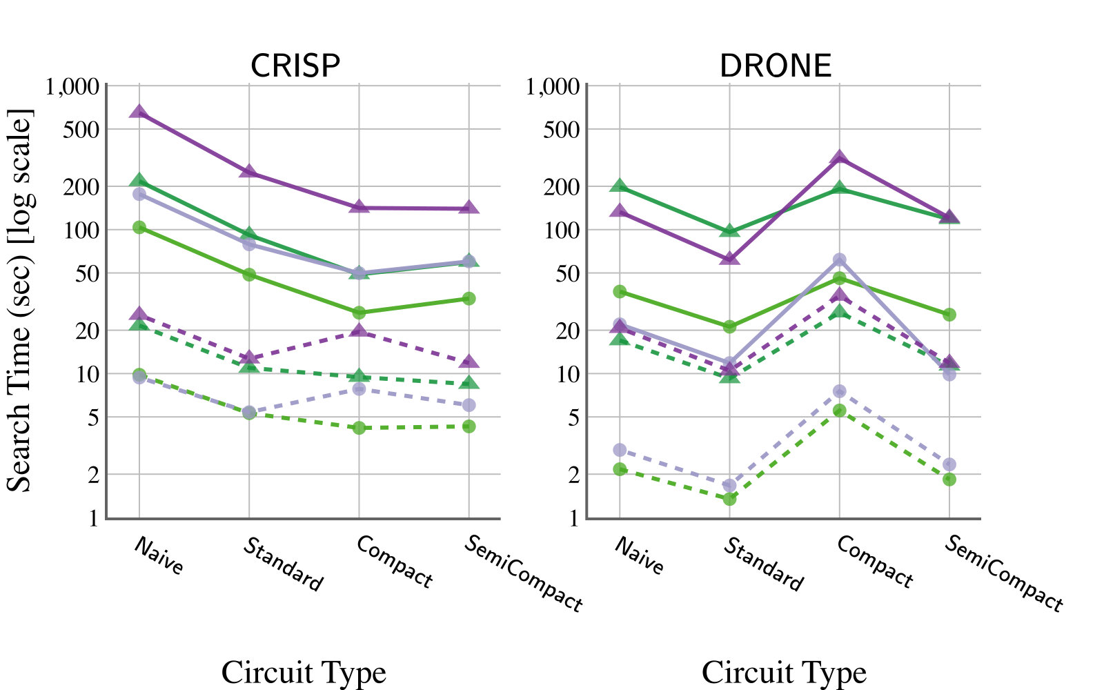
Figure 2: The number of edges in the circuit (left) and average search time (right) for each circuit type.

7 Proof of Main Theorem

Now we are ready to formally state our main result.

Theorem 7.1

If the edge weights are restricted to integers, and there exists a solution with weight at most $\ell\in\mathbb{N}$, then Graph Inspection can be solved in randomized $\tilde{\mathcal{O}}(2^{t}(\ell t^{3}n^{2}+t^{3}|\mathcal{C}|n))$ time and with $\tilde{\mathcal{O}}(\ell tn^{2}+t{|\mathcal{C}|}n)$ space, with a constant success probability.

• Consider running ALG-IPA with CompactCircuit, UnifiedSearch, and MonteCarloRecovery with appropriate preprocessing. We set scaling factor $\lambda=1$, assuming input weights are integral, and let $\theta$ be a constant that controls the overall success probability. The preprocessing steps described in Section 4 take $\tilde{\mathcal{O}}(n^{2})$ time to create a complete, metric graph. Step (1) is optional if we know an upper bound $\ell$ for the solution weight.

  In step (2), as shown by Lemma 5.4, CompactCircuit creates a circuit $\mathcal{F}$ of $\mathcal{O}(\ell t^{2}n+|\mathcal{C}|)$ nodes and $\mathcal{O}(\ell tn^{2}+t|\mathcal{C}|n)$ edges such that if there exists a solution walk with weight at most $\ell$ in $G$, then $\mathcal{F}$ contains a tree certificate for Multilinear Detection with degree at most $t$. This implies that for an output node $O_{\ell^{\prime}}$ for every $\ell^{\prime}\leq\ell$ the fingerprint polynomial $P_{\mathcal{F}[O_{\ell^{\prime}}]}(X,A)$ contains a multilinear monomial with coefficient $1$ if $\ell^{\prime}$ is feasible. Note that $\mathcal{F}$ contains $\mathcal{O}(k)$ addition gates.

  By Lemma 3.5 and Lemma 6.3, we can find the optimal weight $\tilde{\ell}$ in $\tilde{\mathcal{O}}(2^{t}t(\ell tn^{2}+t|\mathcal{C}|n))$ time and $\tilde{\mathcal{O}}(\ell tn^{2}+t|\mathcal{C}|n+t|\mathcal{C}|)=\tilde{\mathcal{O}}(\ell tn^{2}+t|\mathcal{C}|n)$ space with a constant probability. Lastly, in Step (3) we use MonteCarloRecovery to find a solution walk with weight $\tilde{\ell}$. From Lemma 3.6, we can find a tree certificate of $\mathcal{F}$ in $\tilde{\mathcal{O}}(2^{t}t\cdot t(\ell tn^{2}+t|\mathcal{C}|n))=2^{t}(\ell t^{3}n^{2}+t^{3}|\mathcal{C}|n)$ time with a constant probability. As stated in the proof of Lemma 5.3, once we find a tree certificate of $\mathcal{F}$, we can reconstruct a walk $W$ collecting at least $t$ colors with weight $\tilde{\ell}$ on $G$.

  The postprocessing step is to replace each edge $uv$ in $W$ with any of the shortest $u$-$v$ paths in the original graph for Graph Inspection to construct a solution walk $\tilde{W}$. Since $G$ is complete and metric, the weight of $\tilde{W}$ is also $\tilde{\ell}$, and if the edge weight is restricted to (non-negative) integers, this weight is optimal in the original instance. Also, replacing edges in $W$ with shortest paths in the original graph is safe because it is enough to collect colors at the vertices appeared in $W$.

  The algorithm fails only when either UnifiedSearch or MonteCarloRecovery fails. Since both subroutines have a constant success probability, the overall success probability is also constant.         

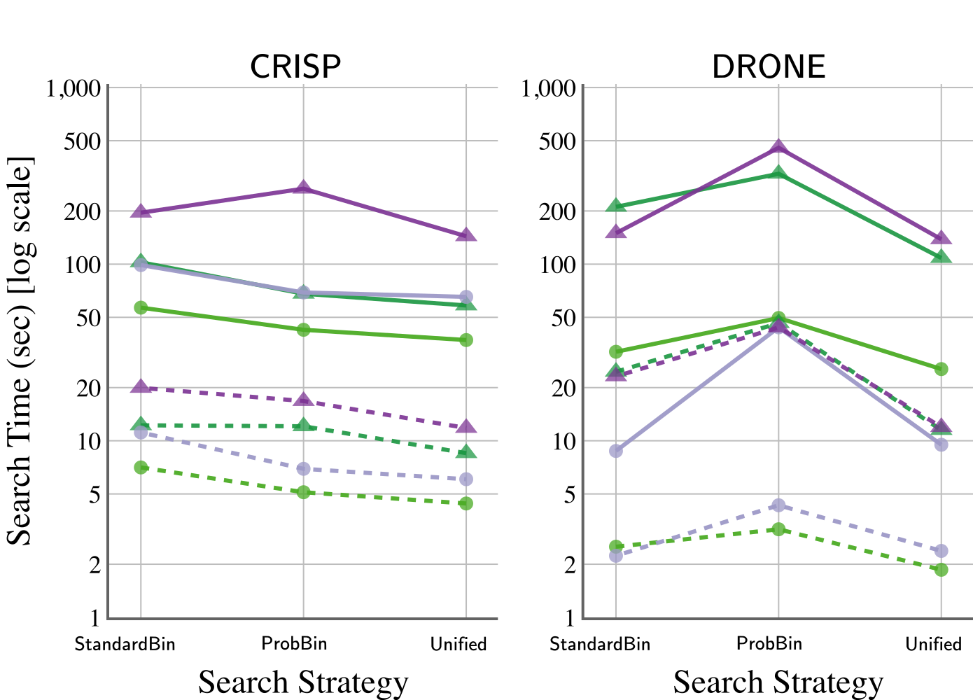
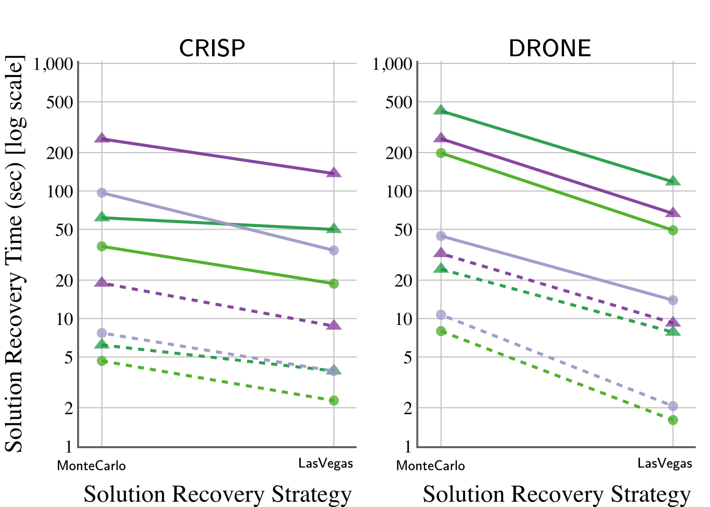
Figure 3: Runtime of each subroutine: search strategies (left) and solution recovery strategies (right).

8 Experimental Results

To show the practicality of our algebraic methods, we conducted computational experiments on the real-world instances used by Fu et al. [6, 5]. We built RRGs (Rapidly-exploring Random Graphs [8]) using IRIS-CLI, originating from the CRISP and DRONE datasets. For each dataset, we created small (roughly $50$ vertex) and large (roughly $100$ vertex) instances and sampled $k\in\{10,12\}$ dispersed POIs (Points Of Interest) using an algorithm from Mizutani et al. [12]. Throughout the experiments, we set $t=k$, i.e. algorithms try to collect all colors (POIs) in the given graph and parallelized using $80$ threads.

We first verify the effect of algorithmic choices—circuit types, search strategies, and solution recovery strategies—to see how they perform on various instances. We tested two scaling factors for each dataset: $\lambda_{\text{small}}=50$, $\lambda_{\text{large}}=100$ for CRISP and $\lambda_{\text{small}}=0.1$, $\lambda_{\text{large}}=0.5$ for DRONE. We measured running times by using the average measurement from three different seeds for a pseudorandom number generator. Next, we tested several scaling factors, as practical instances have real-valued edge weights, to observe trade-offs between running time/space usage and accuracy.

We implemented our code with C++ (using C++17 standard). We ran all experiments on Rocky Linux release 8.8 on identical hardware, equipped with 80 CPUs (Intel(R) Xeon(R) Gold 6230 CPU @ 2.10 GHz) and 191000 MB of memory.

Our code and data to replicate all experiments are available at https://osf.io/4c92e/?view_only=e3d38d9356c04d60b32c2f45ccc19853.

8.1 Choice of Circuit Types.

To assess the four circuit type we proposed in Section 5, we ran our algorithm with all the circuit types, using the UnifiedSearch search strategy. We first measured the number of edges in the constructed arithmetic circuit as this number is a good estimator for running time and space usage.

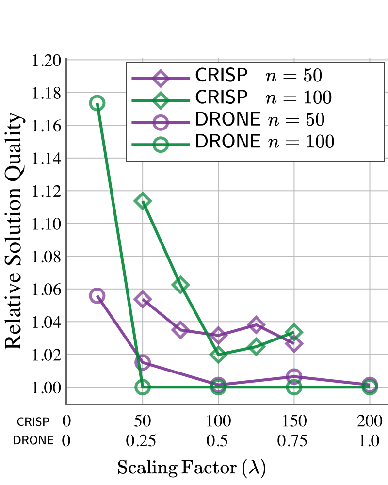
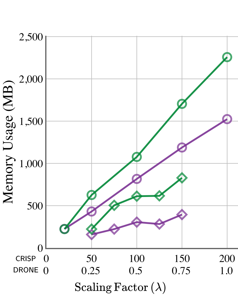
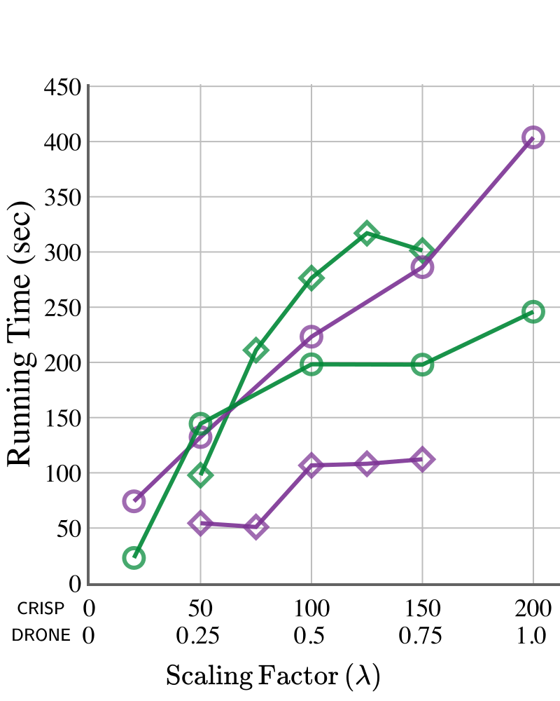
Figure 4: The average ratio of the weight obtained by ALG-IPA to the optimal weight (left), the average peak memory usage (middle), and the average overall running time (right) for different scaling factors.

Figure 2 (left) plots the number of edges of the circuit for each instance. By construction, StandardCircuit always gives a smaller circuit than NaiveCircuit. CompactCircuit has asymptotically the smallest circuit, but in some configurations, especially in DRONE, CompactCircuit results in a larger circuit than StandardBinarySearch. We observed that DRONE has a lower bound higher than that of CRISP, and CompactCircuit has to maintain low-weight walks that are “below” lower bounds, thus creating more edges. Lastly, SemiCompactCircuit has about the same size as StandardCircuit with DRONE and is much smaller with CRISP.

Next, we measured the search time to obtain the optimal weight, using the search strategy UnifiedSearch. Figure 2 (right) plots the average search time for each instance. For both datasets, search time is closely related to the number of edges in the circuit. With the CRISP dataset with larger $k$ ($k=12$), CompactCircuit recorded the best search time. This was not true with DRONE; for that dataset, CompactCircuit is even slower than NaiveCircuit. It is also surprising for us that StandardCircuit performed best on most of the DRONE instances. This suggests that the circuit size is not the only factor for determining the running time.

8.2 Choice of Search Strategies.

For evaluating search strategies, we ran the algorithm with each strategy with the circuit type SemiCompactCircuit and measured the search time (as done in the previous experiment). Figure 3 (left) plots the average search time for various instances. We observe that UnifiedSearch is the fastest with a few exceptions with DRONE, which matches our expectation. ProbabilisticBinarySearch is more unstable; it is faster than StandardBinarySearch with CRISP except $n=100,k=12,\lambda=\lambda_{\text{large}}$, but it is the slowest among three with DRONE.

8.3 Choice of Solution Recovery Strategies.

For each recovery strategy, we measured the time for solution recovery after finding the optimal weight, using circuit type SemiCompactCircuit. As shown in Figure 3 (right), LasVegasRecovery performed better than MonteCarloRecovery with all test instances. Moreover, unlike MonteCarloRecovery, it is guaranteed that LasVegasRecovery always succeeds. We conclude that LasVegasRecovery has clear advantages over MonteCarloRecovery.

8.4 Choice of Scaling Factors.

Finally, we evaluated the effect of varied scaling factors ($\lambda$) by running our algorithm using subroutines SemiCompactCircuit, UnifiedSearch and LasVegasRecovery with fixed $k=12$.

We first measured how the weight of the walk obtained by ALG-IPA is close to the optimal weight. Figure 4 (left) shows the ratio of the weight by ALG-IPA to the optimal (the lower, the better). This ratio was less than $1.2$ for all test instances, and with large enough scaling factors ($100$ for CRISP, $0.25$ for DRONE), the ratio converges within $1.04$. Figure 4 (middle) plots the peak memory usage for ALG-IPA. We observed the almost linear growth of memory usage with respect to the scaling factor. This is due to the fact that the size of an arithmetic circuit is proportional to the solution weight in integers.

Figure 4 (right) shows the overall running time (including search time and solution recovery time) for each instance. The precise running times depend on the structure of an instance as well as randomness, but our experiment demonstrates that running time increases with the scaling factor. Taken together, the plots in Figure 4 illustrate a trade-off between fidelity (influenced by rounding errors) and computational resources (time and space).

8.5 Preprocessing Results

Finally, we present results of preprocessing on our Graph Inspection instances. Because $k$ (the number of colors present in the graph) is small, this preprocessing is quite effective. In particular, removing colorless vertices significantly reduces the size of the graphs.

Table 1: Instance sizes before and after preprocessing. $n_{\text{build}}$ is the parameter given to the software of Fu et al. [6] during instance construction, and can be thought of as a “target” number of vertices for the constructed graph. $k$ is the number of colors remaining after performing color reduction. $n$ and $m$ are the number of vertices and edges in the color-reduced instance, while $n^{\prime}$ and $m^{\prime}$ are the same statistics after preprocessing.

Dataset	$n_{\text{build}}$	$k$	$n$	$m$	$n^{\prime}$	$m^{\prime}$
CRISP	50	10	70	509	15	105
		12			17	136
	100	10	113	951	20	190
		12			24	276
DRONE	50	10	64	329	12	66
		12			14	91
	100	10	119	878	16	120
		12			19	171

9 Conclusion

In this paper we present a novel approach for solution recovery for Multilinear Detection and applied these findings to design a solver for Graph Inspection, thereby addressing real-world applications in robotic motion planning. Using a modular design, we tested variants of different algorithmic subroutines, namely search strategy, circuit design, and solution recovery. Some of our findings are unambiguous and should easily translate to other implementations based on arithmetic circuits: First, we can recommend that parameter search (like the solution weight $\ell$ in our case) is best conducted by constructing a single circuit with multiple outputs for all candidate values. Second, optimizing the circuit design towards size is a clear priority as otherwise the number of circuit edges quickly explodes. Finally, of the two novel solution recovery algorithms for Multilinear Detection, LasVegasRecovery is the clear winner.

Many questions remain open. While our solver is not competitive with the existing solvers on realistic instances of Graph Inspection, it is quite plausible that it can perform well in other problem settings where memory is much more of a concern than running time. One drawback of the current circuit construction is the reliance on the transitive closure of the input graph. A more efficient encoding of the underlying metric graph could substantially reduce the size of the resulting circuit. Further, there might be preprocessing rules for arithmetic circuits that reduce their size without affecting their semantic. Finally, on the theoretical side, we would like to see whether other problems can be solved using the concept of tree certificates.

References

- [1] A. Björklund, P. Kaski, L. Kowalik, and J. Lauri, Engineering motif search for large graphs, in Proceedings of the 17th Workshop on Algorithm Engineering and Experiments (ALENEX), SIAM, 2015, pp. 104–118.
- [2] M. Cygan, F. V. Fomin, Ł. Kowalik, D. Lokshtanov, D. Marx, M. Pilipczuk, M. Pilipczuk, and S. Saurabh, Parameterized algorithms, Springer, 2015.
- [3] R. Diestel, Graph theory, Springer-Verlag, Berlin, 2005.
- [4] B. Englot and F. Hover, Planning complex inspection tasks using redundant roadmaps, in Proceedings of The 15th International Symposium on Robotics Research (ISRR), Springer, 2017, pp. 327–343.
- [5] M. Fu, A. Kuntz, O. Salzman, and R. Alterovitz, Asymptotically optimal inspection planning via efficient near-optimal search on sampled roadmaps, The International Journal of Robotics Research, 42 (2023), pp. 150–175.
- [6] M. Fu, O. Salzman, and R. Alterovitz, Computationally-efficient roadmap-based inspection planning via incremental lazy search, in Proceedings of the 2021 International Conference on Robotics and Automation (ICRA), IEEE, 2021, pp. 7449–7456.
- [7] S. Guillemot and F. Sikora, Finding and counting vertex-colored subtrees, Algorithmica, 65 (2013), pp. 828–844.
- [8] S. Karaman and E. Frazzoli, Sampling-based algorithms for optimal motion planning, The International Journal of Robotics Research, 30 (2011), pp. 846–894.
- [9] P. Kaski, J. Lauri, and S. Thejaswi, Engineering motif search for large motifs, in Proceedings of the 17th International Symposium on Experimental Algorithms (SEA), Schloss Dagstuhl - Leibniz-Zentrum für Informatik, 2018, pp. 28:1–28:19.
- [10] I. Koutis, Faster Algebraic Algorithms for Path and Packing Problems, in Proceedings of the 35th International Colloquium of Automata, Languages and Programming (ICALP), Springer, 2008, pp. 575–586.
- [11] I. Koutis and R. Williams, LIMITS and Applications of Group Algebras for Parameterized Problems, ACM Transactions on Algorithms, 12 (2016), pp. 31:1–31:18.
- [12] Y. Mizutani, D. C. Salomao, A. Crane, M. Bentert, P. G. Drange, F. Reidl, A. Kuntz, and B. D. Sullivan, Leveraging fixed-parameter tractability for robot inspection planning, arXiv preprint arXiv:2407.00251, 2024.
- [13] P. C. Pop, O. Cosma, C. Sabo, and C. P. Sitar, A comprehensive survey on the generalized traveling salesman problem, European Journal of Operational Research, 314 (2024), pp. 819–835.
- [14] R. Williams, Finding paths of length k in time, Information Processing Letters, 109 (2009), pp. 315–318.