CliquePH: Higher-Order Information for Graph Neural Networks through Persistent Homology on Clique Graphs

Abstract

Graph neural networks have become the default choice by practitioners for graph learning tasks such as graph classification and node classification. Nevertheless, popular graph neural network models still struggle to capture higher-order information, i.e., information that goes beyond pairwise interactions. Recent work has shown that persistent homology, a tool from topological data analysis, can enrich graph neural networks with topological information that they otherwise could not capture. Calculating such features is efficient for dimension 0 (connected components) and dimension 1 (cycles). However, when it comes to higher-order structures, it does not scale well, with a complexity of $O(n^{d})$, where $n$ is the number of nodes and $d$ is the order of the structures. In this work, we introduce a novel method that extracts information about higher-order structures in the graph while still using the efficient low-dimensional persistent homology algorithm. On standard benchmark datasets, we show that our method can lead to up to $31\%$ improvements in test accuracy.

1 Introduction

The research area of Graph Neural Networks (GNNs) has received a huge amount of interest in the past few years [1, 2]. As a result, GNNs are now the first choice for many graph-related tasks, like graph classification, node classification, and link prediction. Nevertheless, GNNs present some shortcomings when it comes to modeling higher-order structures (i.e., structures in the graph that go beyond pairwise interactions, like cliques and cycles [3, 4]). In fact, GNNs follow a message-passing framework [5] in which each node communicates with its neighbors, but there is no mechanism to go beyond pairwise interactions, which limits the expressiveness of these models [6]. However, information regarding certain topological structures like cycles and cliques, can be of great importance to graph-related tasks, significantly improving performance [7].

Topological data analysis (TDA) [8] is an emerging area of study that uses techniques from topology, and in particular the tool of persistent homology, to study the shape of the data at multiple scales. TDA is particularly well-suited for capturing higher-order information in graphs, as it can provide information related to structures of different orders, including cliques and cycles, which are known to be particularly informative for several graph-related tasks [7]. Recent works have incorporated topological information related to persistent homology into graph learning tasks with great success [9]. These methods are however limited to persistent homology up to dimension 1, due to the high computational cost that is required for higher dimensions. While this already empowers the model with important structural information that GNNs cannot capture, it is still missing a vast amount of higher-order information.

In this paper we introduce CliquePH, a new topological layer that can be added to any GNN, and that provides information about persistent homology on higher-order structures. Performing persistent homology up to dimension $1$ is extremely efficient and scalable, while higher-dimensional persistent homology is prohibitively expensive [9]. We then devise a strategy that captures higher-order information while still using the efficient low-dimensional persistent homology. In more detail, we first “lift” the graph into multiple clique graphs describing the connections of higher-order structures, and then apply persistent homology up to dimension 1 to each “higher-order” graph. This strategy allows us to use the very efficient (with complexity linear in the number of nodes) persistent homology of dimension 1, while still extracting information from higher-order structures.

The contributions of this paper can be summarized as follows:

• We introduce a topological layer named CliquePH that can be incorporated into any GNN and that provides information related to persistent homology on higher-order graph structures.

• We highlight theoretical results that provide a strong motivation for the use of higher-order persistent homology in graph learning tasks.

• We evaluate our method applied to three popular GNNs on standard graph classification benchmarks, and show performance improvements of up to $31\%$.

2 Preliminaries

We denote a graph with $G=(V,E)$, where $V$ is the set of nodes, with $\lvert V\lvert=n$, and $E$ is the set of edges. We consider attributed graphs, in which every node has a set of $d$ features. The features for each node in a graph are contained in a matrix $\mathbf{X}\in\mathbb{R}^{n\times d}$. We use $\mathcal{N}_{v}$ to indicate the neighbors of node $v$ (i.e., the nodes connected to $v$ by an edge).

Clique Graphs.

A $k$-vertex clique in a graph $G=(V,E)$ is a subset of vertices such that every two distinct vertices in the clique have an edge between them, i.e., $k=\{v_{1},v_{2},\dots,v_{k}\}$, with $v_{i}\in V$, is a $k$-vertex clique if $(v_{i},v_{j})\in E\text{ }\forall i\neq j;\text{ }i,j=1,\dots,k$. Let $k_{1},k_{2},\dots k_{z}$ be the $r$-vertex cliques in the graph $G$, then the $r$-vertex clique graph of $G$ is a graph $K^{(r)}(G)=(V_{K^{(r)}},E_{K^{(r)}})$, with $V_{K^{(r)}}=\{k_{1},k_{2},\dots k_{z}\}$, and $(k_{i},k_{j})\in E_{K^{(r)}}\text{ if and only if }i\neq j\text{ and }k_{i}\cap k_{j}\neq\emptyset$. In other words, the $r$-vertex clique graph $K^{(r)}(G)$ summarizes the structure of the $r$-vertex cliques in the graph $G$.

Table 1: Runtime comparison for one epoch of training of exact higher-order persistent homology up to dimension 2 (denoted with “FullPH”), and our proposed method CliquePH. Results are for the same architecture and hyperparameters trained for one epoch on MNIST dataset. All results are run on NVIDIA A100.

Method Time (h:m:s/epoch) # Iteration/sec Speedup FullPH 9:24:14 0.05 it/s 1 CliquePH 00:02:57 2.42 it/s $\sim$191

Persistent Homology.

Persistent homology [10, 11], a technique for capturing topological features of data, constitutes the foundation of our proposed method. In contrast to other graph learning techniques, persistent homology permits us to quantify topological features at different scales. The crucial element enabling multi-scale calculations is a filtration, i.e., a consistent ordering of the vertices and edges of a graph, defined using a function $f\colon G\to\mathbb{R}$. Filtrations can be either obtained from static descriptor functions that measure certain aspects of a graph, such as its number of connected components or its curvature [12], but recent work also demonstrates that it is possible to learn filtrations in an end-to-end fashion [13, 9]. Regardless of the origin of a filtration, the crucial insight is that, since a graph is a discrete object, its topology can only change at a finite number of critical thresholds $t_{1},\dotsc,t_{k}$. Thus, any function $f\colon G\to\mathbb{R}$ that gives rise to a filtration enables us to turn a graph into a sequence of nested subgraphs $G_{1}\subseteq G_{2}\subseteq\dotsc\subseteq G_{k}=G$, where each $G_{i}$ is defined based on the critical points of $f$ via $G_{i}:=\{x\in V\cup E\mid f(x)\leq t_{i}\}$. Intuitively, each subgraph consists of all elements of the graph $G$ whose function value is less than or equal to the critical threshold. Alongside this sequence of subgraphs, we now calculate the homology groups. These groups capture the topological features—connected components, cycles, voids, and higher-order features—of each subgraph. Persistent homology represents all topological features arising from the filtration in a set of persistence diagrams. Each persistence diagram consists of a multiset of intervals of the form $(c_{i},d_{i})$ with $c_{i},d_{i}\in\mathbb{R}\cup\{\infty\}$, with $c_{i}$ denoting the “creation time” (in terms of the critical thresholds ) and $d_{i}$ denoting the “destruction time.” Features with an infinite destruction time are called essential; these denote topological features that appear at all scales. Prior work in leveraging topological features from graphs ignored clique information due to computational issues: while it is possible to work with higher-order topological features arising from cliques, a naive application of the persistent homology scales with $\mathcal{O}(n^{d})$, where $n$ denotes the number of vertices in a graph, and $d$ denotes the order of cliques (we refer to this as exact higher order persistent homology). Our proposed method instead lifts cliques into individual skeleton graphs, and then performs the efficient persistent homology up to dimension 1. In Table 1 we show a time comparison for one epoch of training, of our proposed method CliquePH with a lifting of the original graph up to 3-vertex clique graphs, and a modified version making use of exact persistent homology up to dimension 2 (dimension 2 corresponds to triangles, i.e., 3-vertex cliques – hence the comparison). The exact persistent homology computations take about 190 times more than our method CliquePH.

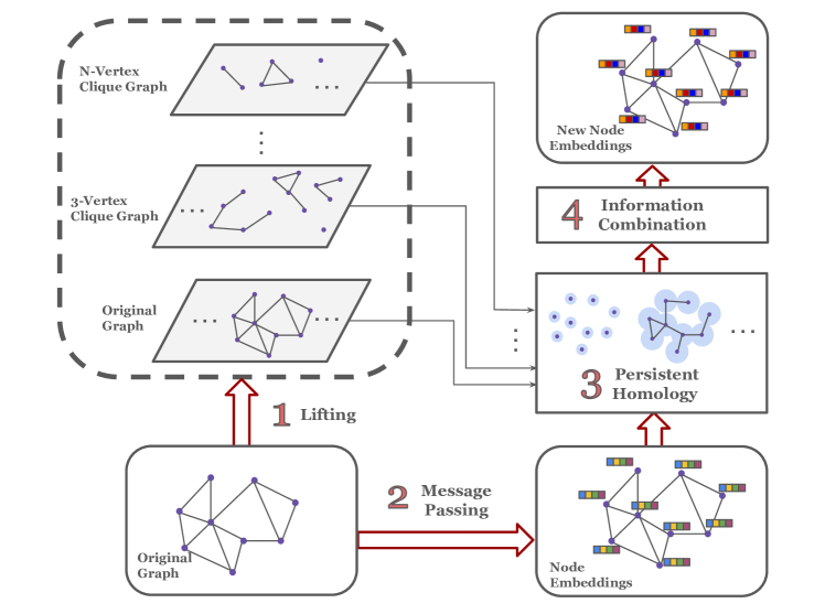
Figure 1: Overview of our method. CliquePH is composed of four stages. (1) First we “lift” the original graph by extracting its clique graphs. (2) We construct node embeddings using a graph neural network. (3) We use learnable functions to generate filtration values for all nodes and edges in all the lifted graphs. We then perform persistent homology (up to dimension 1) on all lifted graphs. (4) We incorporate the information from persistent homology and message-passing into a single representation. The whole model is trained end-to-end.

Graph Neural Networks.

GNNs are deep learning models that operate on graphs. Most popular GNNs adhere to the message-passing framework [5]. Let $\mathbf{H}^{(\ell)}\in\mathbb{R}^{n\times d^{\prime}}$ be the matrix of node representations at iteration $\ell$ (with $\mathbf{H}^{(0)}=\mathbf{X}$, and $\mathbf{H}^{(i)}_{v}$ used to indicate the representation of node $v$ at iteration $i$). Given a permutation-invariant aggregation function $\Phi$, and a learnable update function $\Psi_{\theta}$ (usually a neural network), a message passing layer updates node representations via

$$\mathbf{m}^{(\ell)}_{v} =\Phi(\{\!\{\mathbf{H}_{u}^{(\ell)}\text{ }\lvert\text{ }u\in\mathcal{N}_{v}\}\!\})$$ (1)

$$\mathbf{H}_{v}^{(\ell+1)} =\Psi_{\theta}(\mathbf{H}_{v}^{(\ell)},\mathbf{m}^{(\ell)}_{v})$$ (2)

where $\{\!\{\cdot\}\!\}$ indicates a multiset, and $m_{v}$ is the message received by node $v$ from its neighbours. After $L$ message-passing layers, the node embeddings $\mathbf{H}^{(L)}$ are used to perform a given task (e.g., they are fed to a classifier network), and the whole system is trained end-to-end. For graph-level tasks, it is common to adopt a permutation invariant readout function that aggregates all the node representations into a unique graph embedding (e.g., through averaging).

Topological Graph Neural Networks.

TOGL [9] is a layer that can be added in-between message passing iterations in GNNs to incorporate global topological information extracted by persistent homology up to dimension 1. Given the node embedding at layer $\ell$, TOGL uses a learnable filtration function $f_{\theta}:\mathbf{H}_{v}^{(\ell)}\rightarrow\mathbb{R},\forall v\in V$ to assign a filtration value to each node. Filtration values for each edge are then obtained by taking the maximum filtration value between the two nodes connected by the edge. Successively, persistent homology up to dimension 1 is computed, returning a persistence diagram for dimension $0$ and one for dimension $1$: $\mathcal{D}^{(0)},\mathcal{D}^{(1)}$. The persistence diagrams are then embedded using DeepSet [14] networks $S_{\theta}^{(0)},S_{\theta}^{(1)}$, encoding each diagram into a vector: $\mathbf{A}_{0}=S_{\theta}^{(0)}(\mathcal{D}^{(0)}),\mathbf{A}_{1}=S_{\theta}^{(1)}(\mathcal{D}^{(1)})$. The information from the diagrams is then incorporated into node embeddings (for dimension 0), and to the graph embedding (for dimension 1). All the operations in TOGL are differentiable, and the network is learned end-to-end.

3 Our Method

Our proposed method aims at introducing information from persistent homology on higher-order structures into GNNs. While our method is theoretically different from performing persistent homology up to higher dimensions, we show it brings substantial performance improvements. Our method can be decomposed into four components (as shown in Figure 1), which we present below.

3.1 Graph Lifting

Starting from the original graph $G$, we perform a “lifting“ operation to extract its clique graphs:

$$\text{{lift}}(G)=\{G,K^{(3)}(G),K^{(4)}(G),\dots,K^{(r)}(G)\}$$

the maximum size $r$ for the clique graphs can be defined arbitrarily according to the data at hand (e.g., by taking the value that leads to a clique graph with a number of nodes that is least $5\%$ the number of nodes in the original graph). We start from the $3$-vertex clique graph, as the information about nodes and edges is already present in the original graphs, while the higher dimensions are the ones in which GNNs struggle. This step can be done just once, as pre-processing on all graphs in the dataset.

In practice, we use $r=5$ in our experiments as available datasets tend to have a very small number of cliques larger than that. When dealing with real-world graphs, several works have proposed methods for enumerating all cliques in a graph that in practice have a fast runtime [15, 16, 17, 18]. In all datasets considered in our experiments, we have been able to perform this pre-processing step for each dataset, up to $r=5$, within 1 hour. For instance, complete preprocessing time on MNIST dataset for up to 3-cliques, up to 4-cliques, and up to 5-cliques takes 36.4 min, 58.1 min, and 60.7 min consecutively.

3.2 Message-Passing

In this step, we obtain node embeddings for the original graph $G$. In more detail, we perform $L_{m}$ steps of message passing on $G$. Any GNN could be used for this step, and the output is a matrix of node embeddings $\mathbf{H}^{(L_{m})}$.

3.3 Learnable Persistent Homology

Once we have obtained embeddings for the nodes in $G$, we incorporate information from persistent homology for all graphs in $\text{{lift}}(G)$. This step is composed of three sub-components presented below.

1 - Filtration values for nodes and edges.

To perform persistent homology, we first need to compute filtration values for dimension $0$ (nodes), which we indicate with $\mathbf{F}^{(\cdot)}_{0}$, and dimension $1$ (edges), which we indicate with $\mathbf{F}^{(\cdot)}_{1}$, in all graphs in the lifted set. We first describe how we obtain filtration values for the original graph $G$, and then for the clique graphs $K^{(\cdot)}(G)$.

Original graph $G$. For dimension $0$, we use a two-layer MLP $f_{0}$ to map the embedding of each node into $d_{f}$ filtration values: $\mathbf{F}^{(G)}_{0}(v)=f_{0}(\mathbf{H}_{v}^{(L_{m})})$. For dimension $1$, we first obtain a representation $\mathbf{r}_{e_{i}}$ for each edge $e_{i}=(u,v)$ by concatenating the representations of the nodes it connects: $\mathbf{r}_{e_{i}}=\text{cat}(\mathbf{H}_{v}^{(L_{m})}(u),\mathbf{H}_{v}^{(L_{m})}(v))$. We then obtain the filtration value for the edge using a 2-layer MLP function $f_{1}$ as follows:

$$\mathbf{F}^{(G)}_{1}(e_{i})=max(\{\mathbf{F}^{(G)}_{0}(u),\mathbf{F}^{(G)}_{0}(v)\})+f_{1}(\mathbf{r}_{e_{i}})$$ (3)

Clique graphs $K^{(\cdot)}(G)$. For the lifted graphs, we obtain filtration values in a similar way. Let $k_{i}$ be a node in a clique graph, related to a clique between the nodes $\{u_{1},u_{2},\dots,u_{j}\}$, we first obtain the embedding for $k_{i}$ as $\mathbf{e}_{k_{i}}=\text{cat}(\mathbf{H}_{v}^{(L_{m})}(u_{1}),\dots,\mathbf{H}_{v}^{(L_{m})}(u_{j}))$. We then compute the filtration value as

$$\mathbf{F}^{K^{(\cdot)}}_{0}(k_{i})=\max(\{\mathbf{F}^{(G)}_{0}(u_{1}),\dots,\mathbf{F}^{(G)}_{0}(u_{j})\})+f_{k^{(\cdot)}_{0}}(\mathbf{e}_{k_{i}})$$ (4)

where $f_{k^{(\cdot)}_{0}}$ is a two-layer MLP (a separate one for each clique graph). We then obtain the filtration values for dimension 1 following an analogous procedure to the one used for dimension $1$ on the original graph $G$, using a separate learnable function for each clique graph.

2 - Persistent homology.

We now have filtration values for all the nodes and edges in all the graphs in the lifted set. We can then perform the efficient persistent homology up to dimension 1 to all the graphs, obtaining two persistence diagrams for each graph in the lifted set: $\{(D_{G}^{(0)},D_{G}^{(1)}),(D_{K^{(3)}}^{(0)},D_{K^{(3)}}^{(1)}),\dots,(D_{K^{(r)}}^{(0)},D_{K^{(r)}}^{(1)})\}$. The diagrams for dimension $0$ have a number of entries equal to the number of nodes in the respective graph, while the diagrams for dimension $1$ have a number of entries equal to the number of independent cycles in the respective graph. In other words, these diagrams are summarizing the evolution (according to the learned filtration values) of the connected components and cycles in each graph.

3 - Embed persistence diagrams.

The diagrams for dimension $0$ of the original graph $G$ are passed to a permutation equivariant (set-to-set) DeepSet network (a separate network for each graph in the lifted set is used), which returns a vector for each node. These vectors are stored in a matrix $\mathbf{E}^{(0)}_{G}$. The diagrams for dimension $0$ for all clique graphs are passed to a permutation invariant DeepSet network (a separate network for each clique graph is used), which returns a single vector $\mathbf{E}^{(0)}_{K^{(\cdot)}}$ for each clique graph $K^{(\cdot)}(G)$. The diagrams of dimension $1$ for all graphs are passed through a permutation invariant (set-to-vector) DeepSet network (a separate network for each graph in the lifted set is used) to obtain a unique embedding, which returns a single vector for each graph: $\mathbf{E}^{(1)}_{G},\mathbf{E}^{(1)}_{K^{(3)}},\dots,\mathbf{E}^{(1)}_{K^{(r)}}$.

3.4 Information Combination

We summarize the information from the persistent homology of each clique graph into a unique vector for each dimension. In more detail, we concatenate the vectors $\mathbf{E}^{(0)}_{K^{(\cdot)}}$ and $\mathbf{E}^{(1)}_{K^{(\cdot)}}$, and pass them through a two-layer MLP to obtain a vector $\mathbf{E}_{K^{(j)}}$ for each dimension $j\geq 3$. Finally, we combine all the information from the persistent homology computations with the embeddings obtained in the message passing step. This is done by adding the embeddings together:

$$\mathbf{H}^{(L_{m})} +\mathbf{E}^{(0)}_{G}+\text{{scatter}}(\mathbf{E}^{(1)}_{G})+\text{{scatter}}(\mathbf{E}_{K^{(3)}})+\dots+\text{{scatter}}(\mathbf{E}_{K^{(r)}})$$ (5)

where the function scatter indicates that the embeddings of each clique are added to all the node embeddings of the nodes that form that clique. More formally, given a $3$-vertex clique $k=(u,v,z)$ with embedding $\mathbf{e}_{k}$, the operation $\mathbf{H}+\text{{scatter}}(\mathbf{e}_{k})$ is doing the following

$$\mathbf{H}_{v}=\mathbf{H}_{v}+\mathbf{e}_{k};\text{ }\mathbf{H}_{u}=\mathbf{H}_{u}+\mathbf{e}_{k};\text{ }\mathbf{H}_{z}=\mathbf{H}_{z}+\mathbf{e}_{k}$$ (6)

and leaving the rows of $\mathbf{H}$ related to other nodes unaltered. Additional round(s) of message passing on $G$ can then be performed before passing the embeddings to the final classifier. In the case of a graph-level task, a standard graph pooling method (e.g., averaging) is used.

Finally, we mention that CliquePH does not affect the permutation equivariance of GNNs, and is fully differentiable (hence allowing end-to-end training). More details can be found in Appendix A. We futher provide a comparison between CliquePH and TOGL in Appendix B.

3.5 Limitations

There are three main limitations to our method. Firstly, for very large graphs, it may become difficult computationally to use values of $r$ larger than $3$. While our experiments show that $r=3$ is already enough to provide benefits, this can prevent from exploiting the full potential of CliquePH. Secondly, our method avoids the computational complexity of the exact higher order persistent homology procedure, but it is not equivalent to it, and hence does not have the same theoretical guarantees in terms of expressiveness. Finally, in tasks in which higher-order structures are not informative, CliquePH may not be useful, or may even promote overfitting.

4 Theoretical Motivation

The expressivity of GNNs is measured by considering their ability of distinguishing non-isomorphic graphs. This is done by relating GNNs to the Weisfeiler-Lehman algorithm (or WL algorithm) [19]. We refer to Morris et al. [20] for a complete introduction to WL, its variants, and its use in machine learning. The WL algorithm cannot completely solve the graph isomorphism problem (in fact, there is no known polynomial time solution), but it can still distinguish a large number of graphs [21]. Modifications to the WL algorithm have been made to increase its distinguishing power. In particular, some “higher-order” variants have been proposed. These variants form a hierarchy of algorithms: 1-WL, 2-WL, …, $k$-WL, each more expressive than the previous, i.e., $i$-WL can distinguish more graphs than $(i-1)$-WL. It has been shown that standard message-passing GNNs are strictly less powerful than the 1-WL algorithm [6]. Two recent results, which we provide below, present a strong motivation for using persistent homology to enhance the expressivity of GNNs.

Theorem 4.1 (Persistent Homology is at least as expressive as the 1-WL - Thm. 2 in Horn et al. [9]).

Persistent homology is at least as expressive as the 1-WL algorithm, i.e. if the 1-WL label sequences for two graphs $G$ and $G^{\prime}$ diverge, there exists an injective filtration $f$ such that the corresponding 0-dimensional persistence diagrams $D_{G}^{(0)}$ and $D_{G^{\prime}}^{(0)}$ are not equal.

Theorem 4.2 ($k$-dimensional Persistent Homology is as expressive as $k$-WL - Thm. 3 in Ballester and Rieck [22]).

Given $k$-WL colorings of two graphs $G$ and $G^{\prime}$ that are different, there exists a filtration of $G$ and $G^{\prime}$ such that the corresponding persistence diagrams in dimension $k-1$ or dimension $k$ are different.

Theorem 4.1 entails that first-order persistent homology information can already make any GNN strictly more expressive than the $1$-WL. Theorem 4.2 is a weaker version of this result; it shows that higher-order persistent homology can in fact match the expressiveness of higher-order variants of the WL algorithm—without requiring an enumeration of all $k$-tuples.

As CliquePH makes use of first-order persistent homology information, it is straightforward to see from Theorem 4.1 that a GNN empowered with CliquePH is strictly more powerful than the 1-WL algorithm. While we cannot use Theorem 4.2 to theoretically prove that a version of CliquePH with cliques up to order $k$ leads to the expressiveness of $k$-WL (as CliquePH does not perform exact higher-order persistent homology), we provide below empirical evidence of the practical increase in expressiveness provided by CliquePH.

Empirical Validation of Expressiveness.

We consider 6 datasets of strongly regular graphs [22] (i.e., graphs in which all nodes have the same degree), which are known to be hard to distinguish with the 1-WL test. We then randomly initialize a GCN [23], a GCN with TOGL [9], and a GCN with CliquePH (with a lifting up to 3-vertex clique graphs), and use them to produce graph embeddings. All models are set to have the same number of layers (set to 4), and the internal same dimensionalities (set to 128). We then count the number of unique representations (a network that can distinguish all graphs will provide a different representation for each graph). We show results averaged of 10 random seeds in Table 3. CliquePH increases the capability of distinguishing regular graphs, improving also over TOGL, which has an expressivity strictly higher than the 1-WL, empirically showing that persistent homology information from clique graphs provides important performance benefits.

Table 2: We report the test accuracy (following standard practice, we report ROC-AUC on OGBG-molhiv) obtained on standard benchmark datasets when only structural information is considered (i.e., no node attributes are used). We compare standard popular GNNs (GCN, GIN, GAT) alone, and with the addition of TOGL and our proposed method, CliquePH. The highest performing model of each dataset is highlighted with a grey background and the highest performing variant for each architecture in bold. The last column on the right shows the average performance improvement provided by TOGL and CliquePH with respect to the base GNN.

Graph classification Method DD ENZYMES MNIST PROTEINS IMDB-B REDDIT-5K OGBG-molhiv Avg. $\uparrow$ GCN-4 ${68.0}\pm{3.6}$ ${22.0}\pm{3.3}$ ${76.2}\pm{0.5}$ ${68.8}\pm{2.8}$ ${65.1}\pm{5.1}$ ${54.1}\pm{0.8}$ ${66.4}\pm{1.8}$ ${-}$ GCN-3-TOGL-1 ${75.1}\pm{2.1}$ ${30.3}\pm{6.5}$ ${84.8}\pm{0.4}$ ${73.8}\pm{4.3}$ ${72.5}\pm{3.0}$ ${54.3}\pm{1.4}$ ${69.4}\pm{1.8}$ ${5.7}$ GCN-3-CliquePH-1 ${76.1}\pm{1.3}$ ${34.3}\pm{4.7}$ ${83.6}\pm{0.7}$ ${72.6}\pm{1.5}$ ${74.7}\pm{1.2}$ ${57.7}\pm{0.5}$ ${69.6}\pm{2.0}$ ${6.9}$ GIN-4 ${75.6}\pm{2.8}$ ${21.3}\pm{6.5}$ ${83.4}\pm{0.9}$ ${74.6}\pm{3.1}$ ${71.1}\pm{3.7}$ ${50.2}\pm{2.4}$ ${68.7}\pm{0.9}$ ${-}$ GIN-3-TOGL-1 ${76.2}\pm{2.4}$ ${23.7}\pm{6.9}$ ${84.4}\pm{1.1}$ ${73.9}\pm{4.9}$ ${74.4}\pm{1.6}$ ${52.7}\pm{0.9}$ ${65.1}\pm{6.2}$ ${0.8}$ GIN-3-CliquePH-1 ${77.6}\pm{1.7}$ ${24.7}\pm{3.1}$ ${88.9}\pm{0.6}$ ${72.9}\pm{0.9}$ ${72.4}\pm{2.8}$ ${55.0}\pm{1.4}$ ${69.6}\pm{1.8}$ ${2.3}$ GAT-4 ${63.3}\pm{3.7}$ ${21.7}\pm{2.9}$ ${63.2}\pm{10.4}$ ${67.5}\pm{2.6}$ ${63.6}\pm{3.9}$ ${48.1}\pm{1.1}$ ${51.8}\pm{5.6}$ ${-}$ GAT-3-TOGL-1 ${75.7}\pm{2.1}$ ${23.5}\pm{6.1}$ ${77.2}\pm{10.5}$ ${72.4}\pm{4.6}$ ${71.2}\pm{2.4}$ ${52.7}\pm{1.4}$ ${68.6}\pm{1.7}$ ${8.8}$ GAT-3-CliquePH-1 ${75.2}\pm{1.9}$ ${27.5}\pm{4.0}$ ${83.8}\pm{0.9}$ ${72.6}\pm{0.8}$ ${71.5}\pm{2.6}$ ${53.7}\pm{1.0}$ ${69.9}\pm{1.7}$ ${10.7}$

Table 3: Number of strongly regular graphs distinguishable by untrained models. All models have the same number of layers and dimensionality. CliquePH can enhance the ability of networks to distinguish “hard” non-isomorphic graphs.

Dataset	Cubic12	Cubic14	Cubic16	Quartic10	Quartic11	Quartic12
# Graphs	85	509	4060	59	265	1544
GCN	${78}\pm{0.0}$	${458}\pm{0.0}$	${3604}\pm{0.0}$	${56}\pm{0.0}$	${255}\pm{0.0}$	${1427}\pm{0.0}$
GCN-TOGL	${85}\pm{0.0}$	${507.2}\pm{1.4}$	${4049.4}\pm{3.7}$	${59}\pm{0.0}$	${264}\pm{0.0}$	${1540.1}\pm{2.1}$
GCN-CliquePH	${85}\pm{0.0}$	${509}\pm{0.0}$	${4057.1}\pm{0.7}$	${59}\pm{0.0}$	${265}\pm{0.0}$	${1542.3}\pm{2.21}$

5 Experiments

To demonstrate the benefits provided by our method in practical scenarios, we follow prior literature [9] and apply our method to three GNNs among the most used by practitioners: GCN [23], GIN [6], and GAT [24]. In more detail, we report results for each GNN by itself, for the GNN with the addition of TOGL [9], and for the GNN with the addition of our method CliquePH. The comparison with TOGL is particularly useful, as TOGL is a topological method that can be used on top of any GNN (like CliquePH), and it makes use of information coming from persistent homology up to dimension one. This then allows us to analyze the benefit provided by the persistent homology information obtained from the higher-order clique graphs that is present in our method. Finally, we provide an ablation study to observe the effects of the position of the CliquePH layer in the model architecture.

Experimental Setup and Datasets.

In order to ensure a fair performance comparison, we take the optimal architectures and hyperparameters for the GNNs and for TOGL from prior work [9]. For CliquePH we use the same architecture for the base GNN of TOGL, and we tune only the learning rate and the maximum dimension of the lifted clique graphs (between 3, 4, and 5) using a random search approach (using values in the interval: $(10^{-6},10^{-2})$) by comparing the loss on the validation set. Furthermore, the reported results are obtained by averaging over ten independent runs with varying random seeds. The code to replicate our experiments will be publicly released upon acceptance. In Tables 2 and 4, the notation “GCN-4” indicates a GCN architecture with 4 message passing layers, while “GCN-3-CliquePH-1” indicates a GCN architecture with 3 message passing layers, and 1 CliquePH layer. We use the analogous notation for the other GNNs, and for networks with TOGL. All experimental results were conducted on a single NVIDIA A100 GPU, and 20 allocated AMD EPYC 7742 64-Core CPUs, with the Adam optimizer, 4 workers, and a batch size of 32 for small datasets and 128 for large datasets. We use standard graph classification benchmark datasets: DD [25], ENZYMES [26], MNIST [27], PROTEINS [28], IMDB-B [29], Reddit-5k [30], and OGBG-Molhiv [31]. We perform two types of experiments, the first, which we refer to as structure-based, does not consider the information coming from node features; the second instead follows the standard procedure, and makes use of the available node attributes. To ensure the same training, evaluation, and data setup, we use the code provided by the authors of TOGL [9], and we report results for TOGL and base models from their paper.

Performance on Structure-based Experiments.

Following prior work [9], to perform structure-based experiments, we assign random node labels and input features. This approach allows us to assess the practical effectiveness of our method in comparison to classical message-passing GNNs for extracting underlying structural and topological information. Table 2 shows the results for the structure-based graph classification task. Firstly, we observe that CliquePH and TOGL significantly improve the performance of standard GNNs. CliquePh in particular leads to the highest average improvement across datasets (last column on the right), with an improvement of $6.9\%$ with respect to the base GCN model, $2.3\%$ with respect to the base GIN, and $10.7\%$ with respect to the base GAT. Looking at individual datasets, we then notice that a CliquePH model is the best performing model on 6 out of 7 datasets. Furthermore, it can be seen that in most cases, the results for CliquePH present a lower variance across runs, showing an increased stability with respect to TOGL.

Performance on Benchmark Datasets.

We now investigate the effect of CliquePH layer on standard benchmark datasets making use of node attributes. We use the same datasets used for the structure-based experiments, except for MNIST, which does not have node attributes. Results are shown in Table 4. We notice that CliquePH can significantly improve the performance of GNNs even in the presence of rich feature information, while this is not the case for TOGL. In fact, the average performance improvement across datasets for CliquePH is always positive (while for TOGL it is negative for the GIN model) and in $90\%$ of the cases, the addition of CliquePH improves the performance of the baseline GNN, with improvements of up to $31\%$. As above, we notice that in the majority of cases, the results for CliquePH have a lower variance than the ones for TOGL, highlighting the increased stability of our method.

Table 4: We report the test accuracy (following standard practice, we report ROC-AUC on OGBG-molhiv) obtained on standard graph classification benchmark datasets (considering node features). We compare standard popular GNNs (GCN, GIN, GAT) alone, and with the addition of TOGL and our proposed method, CliquePH. The highest performing model of each dataset is highlighted with grey background and the highest performing variant for each architecture in bold. The last column on the right shows the average performance improvement provided by TOGL and CliquePH with respect to the base GNN.

Graph classification Method DD ENZYMES MNIST PROTEINS-FULL IMDB-B REDDIT-5K OGBG-molhiv Avg. $\uparrow$ GCN-4 ${72.8}\pm{4.1}$ ${58.3}\pm{6.1}$ ${90.0}\pm{0.3}$ ${76.1}\pm{2.4}$ ${68.6}\pm{4.9}$ ${53.7}\pm{1.7}$ ${71.9}\pm{1.1}$ ${-}$ GCN-3-TOGL-1 ${73.2}\pm{4.7}$ ${53.0}\pm{9.2}$ ${95.5}\pm{0.2}$ ${76.0}\pm{3.9}$ ${72.8}\pm{2.3}$ ${54.5}\pm{1.2}$ ${72.6}\pm{2.0}$ ${0.9}$ GCN-3-CliquePH-1 ${75.0}\pm{1.8}$ ${55.5}\pm{4.2}$ ${95.9}\pm{0.2}$ ${82.0}\pm{0.5}$ ${71.1}\pm{3.2}$ ${55.6}\pm{1.2}$ ${75.2}\pm{2.3}$ ${2.7}$ GIN-4 ${70.8}\pm{3.8}$ ${50.0}\pm{12.3}$ ${96.1}\pm{0.3}$ ${72.3}\pm{3.3}$ ${72.8}\pm{2.5}$ ${53.3}\pm{1.6}$ ${69.8}\pm{1.1}$ ${-}$ GIN-3-TOGL-1 ${75.2}\pm{4.2}$ ${43.8}\pm{7.9}$ ${96.1}\pm{0.1}$ ${73.6}\pm{4.8}$ ${74.2}\pm{4.2}$ ${53.7}\pm{1.1}$ ${67.3}\pm{4.0}$ ${-0.17}$ GIN-3-CliquePH-1 ${76.1}\pm{2.6}$ ${54.8}\pm{8.4}$ ${96.3}\pm{0.1}$ ${81.4}\pm{1.1}$ ${73.7}\pm{2.1}$ ${55.1}\pm{1.7}$ ${72.9}\pm{1.6}$ ${3.6}$ GAT-4 ${71.1}\pm{3.1}$ ${26.8}\pm{4.1}$ ${94.1}\pm{0.3}$ ${71.3}\pm{5.4}$ ${73.2}\pm{4.1}$ ${51.4}\pm{1.4}$ ${74.0}\pm{2.1}$ ${-}$ GAT-3-TOGL-1 ${73.7}\pm{2.9}$ ${51.5}\pm{7.3}$ ${95.9}\pm{0.3}$ ${75.2}\pm{3.9}$ ${70.8}\pm{8.0}$ ${52.5}\pm{0.9}$ ${74.7}\pm{1.8}$ ${4.6}$ GAT-3-CliquePH-1 ${75.4}\pm{3.1}$ ${57.5}\pm{9.2}$ ${96.8}\pm{0.2}$ ${80.8}\pm{1.4}$ ${70.7}\pm{3.0}$ ${53.8}\pm{1.5}$ ${75.7}\pm{1.1}$ ${7.0}$

Ablation Study.

We investigate the effects of the position of the CliquePH layer inside a GNN architecture, and the maximum dimension $r$ of the lifted clique graphs. We provide below an overview of the results and we refer to Appendix C for the full results. We start by considering a 4-layer GNN, with 3 message passing layers and 1 CliquePH layer, and we change the position of the latter. We consider the structure-based scenario to exclude the influence of node features. Results are shown in Figure 2 (Left) for the DD dataset (other datasets are in the Appendix). We notice that the effects are highly dataset dependent: for DD using CliquePH as the first layer is more effective, while, e.g., for Enzymes the best performance is when the layer is 3rd, similar to PROTEINS. We then consider a GNN with a number of layers that vary from 1 to 5 and with CliquePH as the last layer. Results are shown in Figure 2 (Center). Again we notice that the performance is highly dependent on the dataset, as for DD there is little change in performance for different numbers of layers, while, e.g., for ENZYMES it is important to have 2 to 4 layers prior to CliquePH. On IMDB-B we notice how the addition of CliquePH significantly increases performance even for a 1-layer architecture. Finally, we notice how in all cases the addition of CliquePH always leads to performance improvements. Finally, we apply CliquePH with a maximum dimension of the lifted clique graphs varying from 3 to 5 on the DD dataset. Results are shown in Figure 2 (Right). We observe that tuning this parameter is important to avoid overfitting. These results suggest that tuning the position of CliquePH, and the value of $r$, is important to obtain the best results, and that CliquePH always leads to performance improvements when no node features are available.

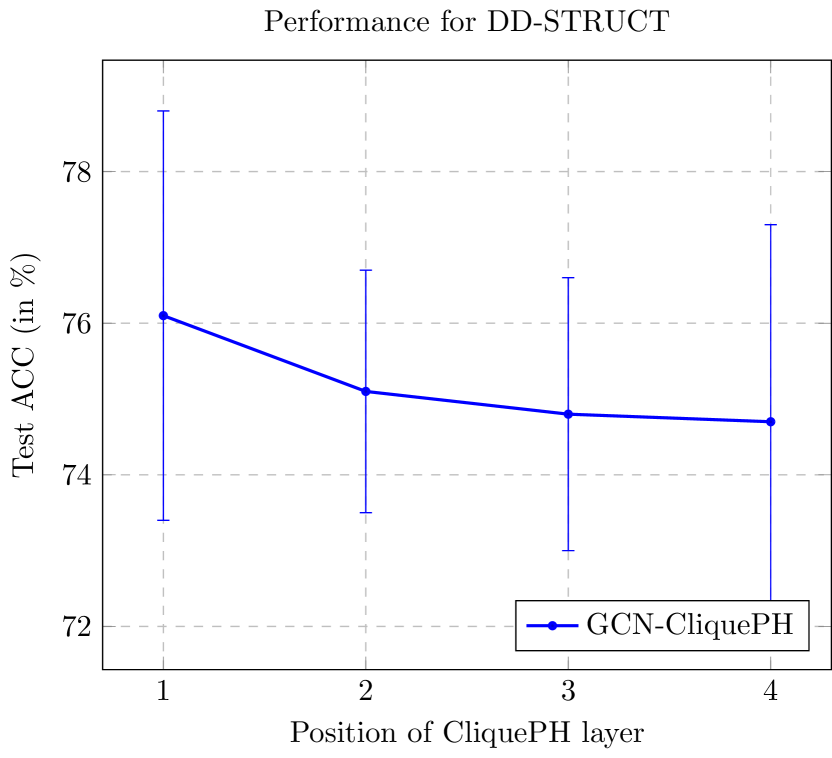
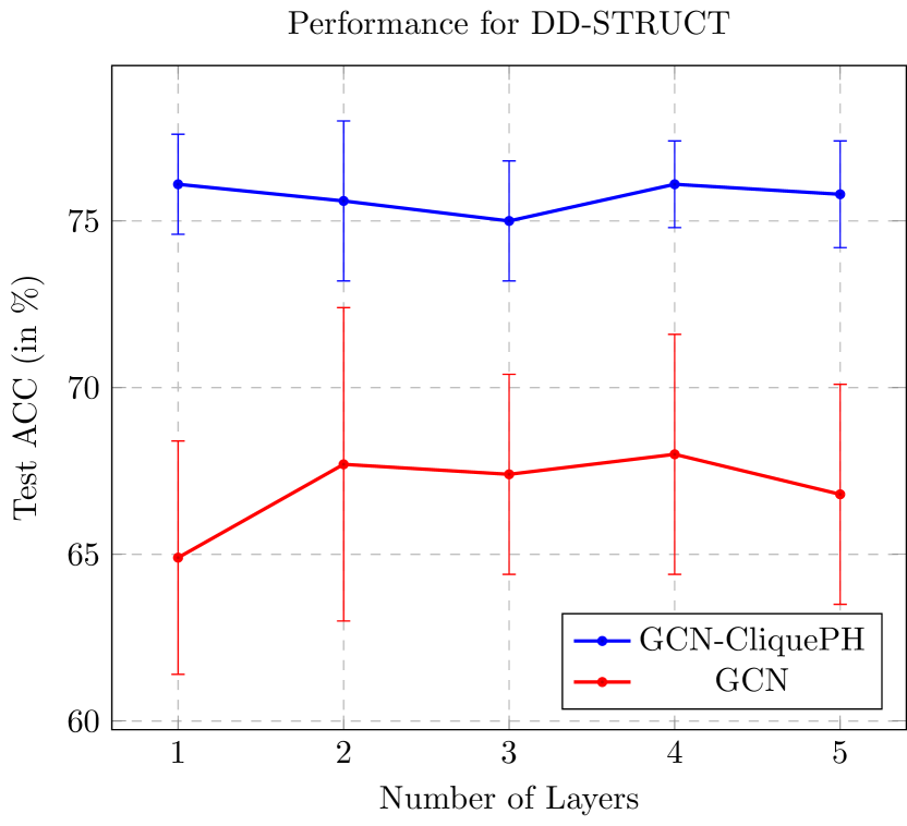
Figure 2: Ablation Results for different architectures. (Left) Test accuracy for the structure-based experiments while changing the position of CliquePH layer. (Center) Test accuracy for the structure-based experiments while increasing the total number of layers in the model. Error bars show standard deviation over 10 runs. (Right) Test accuracy for the structure-based experiments while changing the maximum dimension of the lifted clique graphs of CliquePH.

6 Related Work

Graph neural networks and topological data analysis have become very popular and prolific research fields. In this section, we review works at the intersection of graph machine learning and topology, and we refer the interested reader to comprehensive surveys for the latest advancements in graph neural networks [1, 2] and topological data analysis [32, 33, 34]. In the context of graph neural networks augmented with topological information, Bouritsas et al. [7] show that adding information about the number of higher-order structures that a node belongs to can improve the theoretical expressivity and practical performance of a model. Similarly, Immonen et al. [35] use a topological descriptor based on filtrations as additional node features for GNNs. Zhao et al. [36] use persistent homology to weight messages in GNNs in the message passing procedure. He et al. [37] use sheaf theory to produce node position encodings that improve the performance of graph neural networks on several tasks. Song et al. [38] propose a feature augmentation method by obtaining topology embedding of nodes through Node2vec. This introduces topological structure information into an end-to-end model to improve node representation learning. In addition, several works discuss message-passing on topological spaces. Bodnar et al. [39] introduce a model that performs message passing over simplicial complexes. Bodnar et al. [40] successively extended this model to cellular complexes. Later work [41] has also introduced models that operate on cellular sheaves. While these works are related to CliquePH, there are some important differences. Firstly, these methods require a specific message-passing model, while our method CliquePH can be applied in conjunction with any existing GNN. Secondly, CliquePH makes use of Persistent Homology, which provides access to information (e.g., the exact number of cliques and cycles in the original graph and in each lifted graph) that cannot be guaranteed to be accessible to methods that perform message passing on topological structures. Finally, several works also focus on the explicit connections between topological data analysis and graph learning. O’Bray et al. [42] use graph filtrations to compute efficient graph representations that can outperform those obtained from GNNs. Southern et al. [43] leverage topological tools to robustly evaluate generative graph models. Coupette et al. [44] introduces the concept of curvature for hypergraphs and show that they can be used to effectively perform clustering. Carriere et al. [45] use extended persistent diagrams to produce graph embeddings. Srambical and Rieck [46] use graph filtrations to classify dynamic graphs. Ye et al. [47] introduces the use of extended persistent homology, a variant of persistent homology, into graph-related tasks.

7 Conclusions

GNNs are powerful models operating on graph structures, but they lack the ability of extracting information about higher-order structures. In this paper, we introduce a novel learnable topological layer that provides GNNs with information from persistent homology on higher-order structures present in a graph. Our experimental results show that our method leads to performance improvements of up to $31\%$ on standard benchmarks for the tasks of graph classification.

Appendix A Permutation Equivariance & Differentiability

Permutation Equivariance.

Most popular GNNs are permutation equivariant (as we do not want the ordering of the nodes to affect the final output), and it is hence important to address whether our proposed method impacts this property. Assuming the use of a permutation equivariant GNN for the message passing operations in CliquPH, and noticing that persistent homology is permutation equivariant by design, we can confirm that CliquePH does indeed preserve this property.

Differentiability.

The persistent homology computations are differentiable (and hence allow end-to-end training) only with an appropriate choice of function to embed the persistence diagrams. In particular, we refer to the following theorem from Horn et al. [9, Theorem 1].

Theorem A.1.

Let $f_{\theta}$ be a vertex filtration function $f_{\theta}:V\rightarrow R$ with continuous parameters $\theta$, and let $\Psi$ be a differentiable embedding function (used to embed persistence diagrams) of unspecified dimensions. If the vertex function values of $f_{\theta}$ are distinct for a specific set of parameters $\theta^{\prime}$, i.e. $f_{\theta}(v)\neq f_{\theta}(w)\text{ for }v\neq w$, then the map $\theta\rightarrow\Psi(\text{ph}(G,f_{\theta}))$ is differentiable at $\theta$.

Differentiability thus hinges on unique function values at the vertices of the graph. We observe that this condition is always satisfied in practice (as the chances of having all floating point values be exactly the same are infinitesimally small); if need be, it can be enforced by a random perturbation of function values, similar to the well known strategy of adding random features to GNNs [48, 49]. Since we use DeepSet (which is a differentiable architecture) as our function to embed the persistence diagrams, we are guaranteed to be respecting Theorem A.1, thus ensuring the differentiability of our CliquePH method.

Appendix B Differences Between CliquePH and TOGL

Our method CliquePH is strictly related to TOGL [9] as both methods provide a “plug-in” topological layer for GNNs. Furthermore, both methods rely on a differentiable (and learnable) implementation of persistent homology as the main tool for capturing topological information.

There are however several differences which we highlight below

• CliquePH introduces a lifting operation that allows the model to obtain persistent homology information on the clique graphs representing the connectivity of higher-order structure in the graph. TOGL on the other hand is strictly limited to information up to dimension 1. This point implies that CliquePH has several functions that are not present in TOGL (e.g., the functions for computing filtration values for the lifted graphs, the functions for embedding higher-order persistence diagrams, the functions for combining information from lifted graphs).

• In eq. 3, the learnable function $f_{1}$ is not present in the original TOGL layer, and provides CliquePH with more flexibility. In fact, this provides the model with an additional learnable function that can modify the filtration value of the edge without modifying the values for the nodes connected by that edge.

• CliquePH uses an MLP for combining information (section 3.4) from persistence diagrams into node embeddings. TOGL does not use a learnable function for this step.

Appendix C Full Ablation results

We start by considering a 4-layer GNN, with 3 message passing layers and 1 CliquePH layer, and we change the position of the latter. We consider the structure-based scenario to exclude the influence of node features. Results are shown in Figure 3 (Center) for the DD, ENZYMES, and PROTEINS datasets. We notice that the effects are highly dataset dependent: for DD using CliquePH as the first layer is more effective, while for Enzymes the best performance is when the layer is 3rd, similar to PROTEINS.

We then consider a GNN with a number of layers that vary from 1 to 5 and with CliquePH as the last layer. Results are shown in Figure 4. Again we notice that the performance is highly dependent on the dataset, as for DD there is little change in performance for different numbers of layers, while for ENZYMES it is important to have 2 to 4 layers prior to CliquePH. On PROTEINS we notice how the addition of CliquePH significantly increases performance even for a 1-layer architecture. Finally, we notice how in all cases the addition of CliquePH always improves the final performance.

Finally, in Figure 5 we show the performance of a GCN, GIN, and GAT model with different maximum dimension of the lifted graph (varying between 3, 4, and 5) on the DD dataset in a structure-based setting. The results confirm the importance of tuning this parameter to avoid overfitting the data. We also notice that GIN, the theoretically most expressive architecture of the three, achieves the highest performance with a maximum dimension of 4, while GCN and GAT prefer 3.

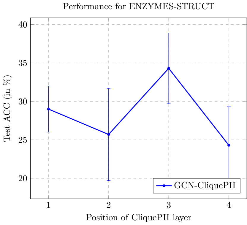
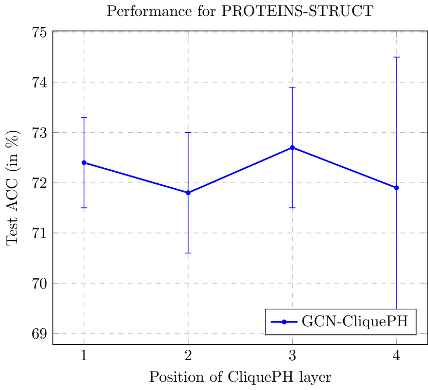
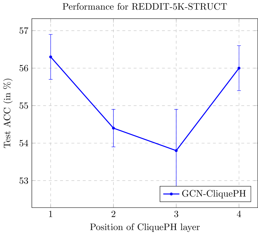
Figure 3: Comparison of test accuracy for the structure-based experiments while changing the position of CliquePH layer in the GCN model architecture. Results averaged over 10 runs.

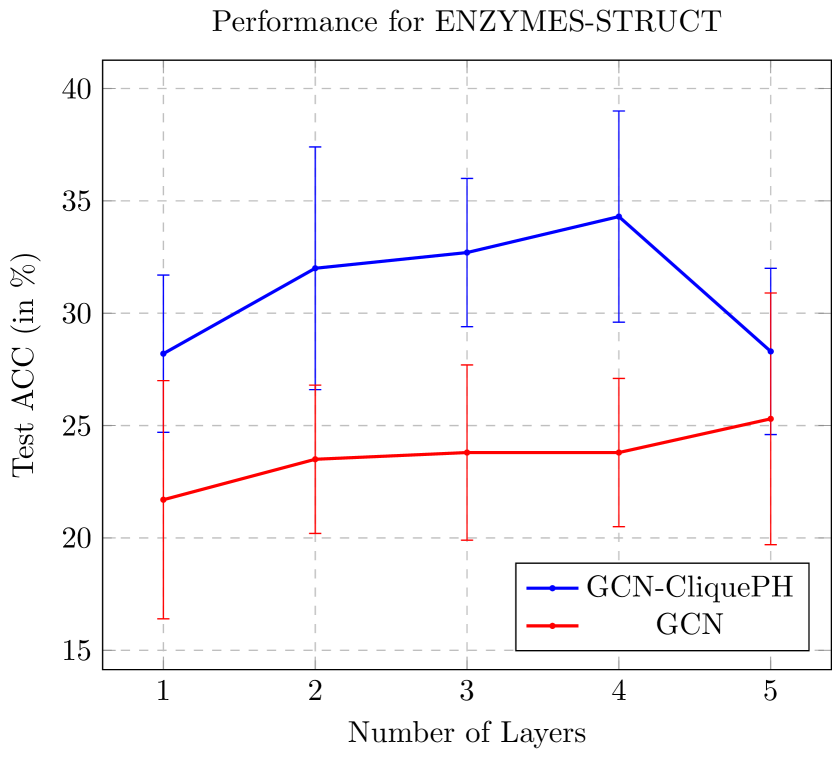
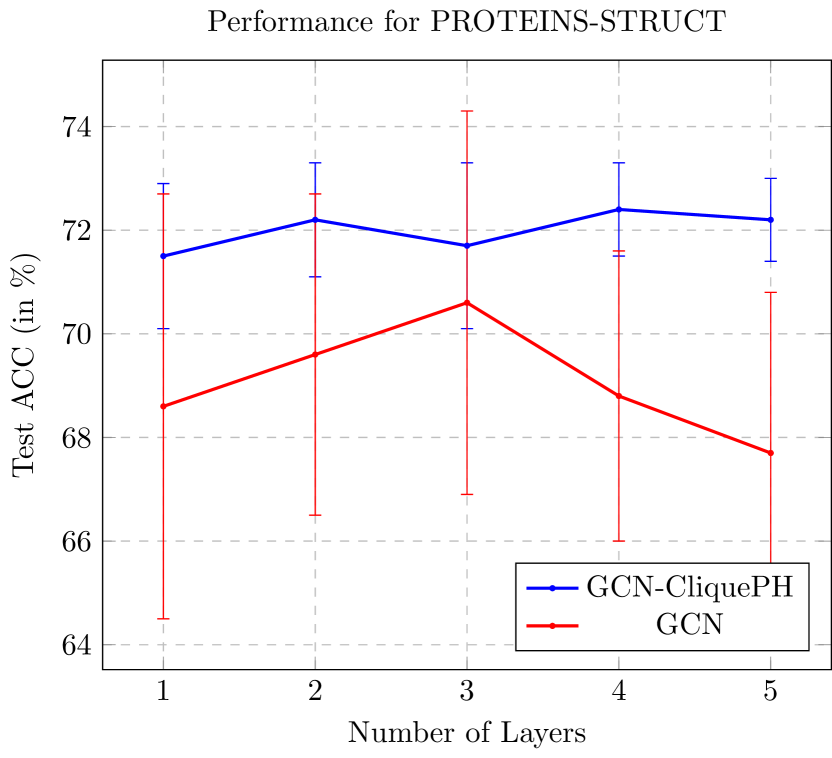
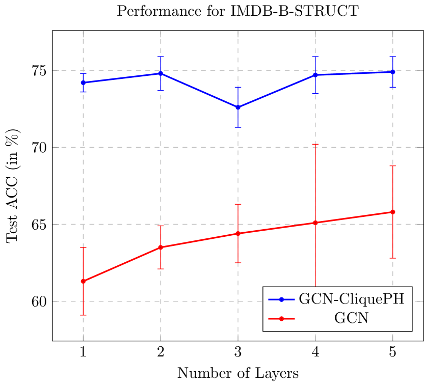
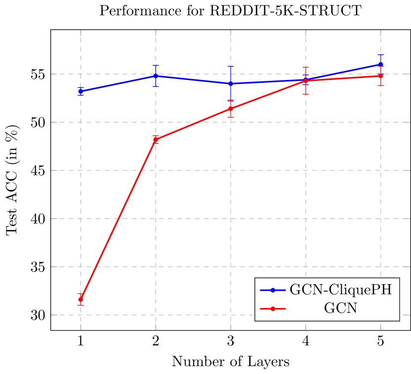
Figure 4: Comparison of test accuracy for the structure-based experiments while increasing the total number of layers in the model architecture. Error bars show the standard deviation over 10 runs.

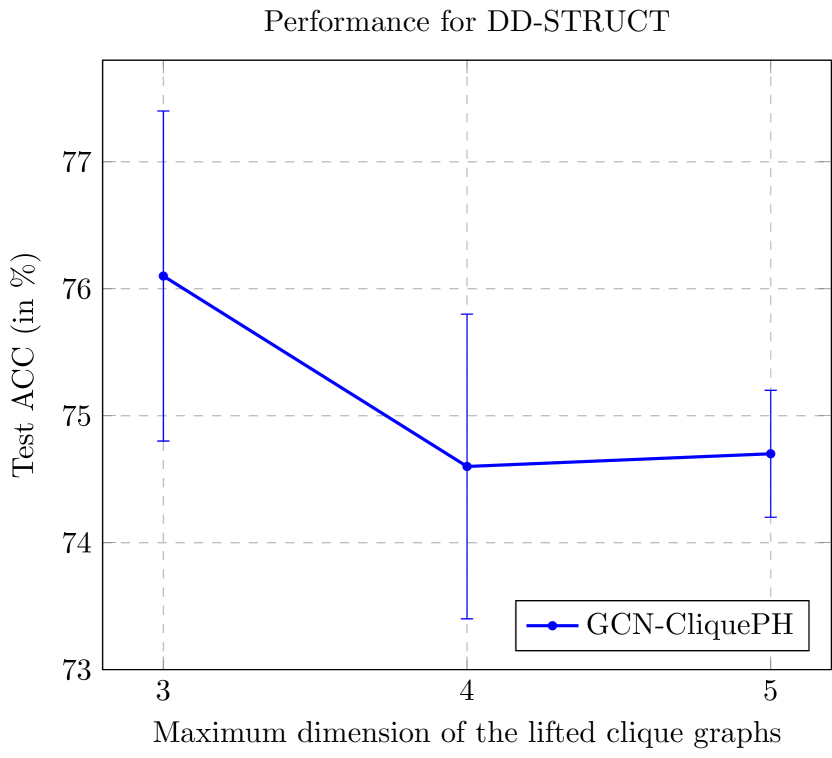
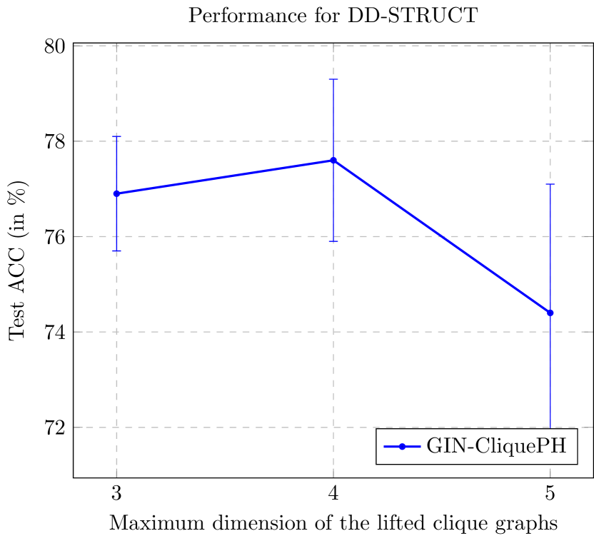
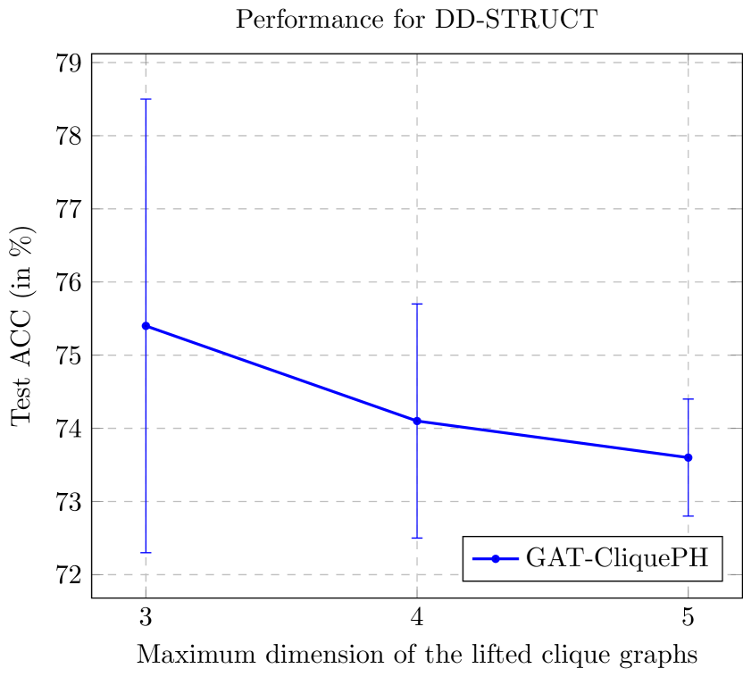
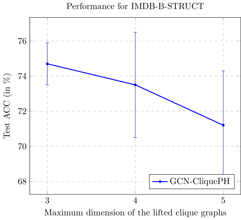
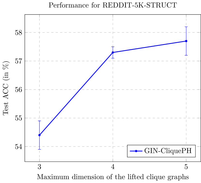
Figure 5: Comparison of test accuracy for the structure-based experiments while changing the maximum dimension of the lifted clique graphs of CliquePH. Results averaged over 10 runs.

Appendix D Node Classification Experiments

While we believe the benefits of CliquePH are more visible for graph classification tasks (in which higher-order structural information usually plays a much more important role), we performed a small experiment on the Cora-ML [50], Coauthor CS [51], and Coauthor Physics [51] datasets. We followed the same practices and architectures we used for the graph classification datasets plus an additional 0.2 drop-out on all architectures to prevent overfitting. We adhered to the widely accepted practice of training-validation-test splits of 60%-20%-20%. We report results in Table 5, and show that CliquePH can provide benefits also for node-level tasks.

Table 5: We report the test accuracy for node classification. We compare standard popular GNNs (GCN, GIN, GAT) alone, and with the addition of TOGL and our proposed method, CliquePH. The highest performing model of each dataset is highlighted with grey background and the highest performing variant for each architecture in bold.

Method Cora-ML Coauthor CS Coauthor Physics GCN-4 ${92.4}\pm{0.8}$ ${92.9}\pm{0.1}$ ${96.1}\pm{0.06}$ GCN-3-TOGL-1 ${93.0}\pm{1.1}$ ${93.0}\pm{0.1}$ ${96.4}\pm{0.06}$ GCN-3-CliquePH-1 ${93.4}\pm{0.6}$ ${93.7}\pm{0.3}$ ${96.6}\pm{0.07}$ GIN-4 ${92.9}\pm{1.3}$ ${92.6}\pm{0.2}$ ${95.9}\pm{0.1}$ GIN-3-TOGL-1 ${93.2}\pm{0.6}$ ${93.2}\pm{0.3}$ ${96.3}\pm{0.05}$ GIN-3-CliquePH-1 ${94.2}\pm{1.0}$ ${94.3}\pm{0.3}$ ${96.4}\pm{0.01}$ GAT-4 ${93.7}\pm{1.2}$ ${93.2}\pm{0.2}$ ${96.2}\pm{0.2}$ GAT-3-TOGL-1 ${93.8}\pm{0.7}$ ${93.3}\pm{0.4}$ ${96.1}\pm{0.2}$ GAT-3-CliquePH-1 ${94.4}\pm{0.8}$ ${94.3}\pm{0.3}$ ${96.4}\pm{0.07}$

References

- Waikhom and Patgiri [2023] Lilapati Waikhom and Ripon Patgiri. A survey of graph neural networks in various learning paradigms: methods, applications, and challenges. Artificial Intelligence Review, 56(7):6295–6364, 2023.
- Wu et al. [2020] Zonghan Wu, Shirui Pan, Fengwen Chen, Guodong Long, Chengqi Zhang, and S Yu Philip. A comprehensive survey on graph neural networks. IEEE transactions on neural networks and learning systems, 32(1):4–24, 2020.
- Diestel et al. [2008] Reinhard Diestel, Alexander Schrijver, and Paul Seymour. Graph theory. Oberwolfach Reports, 4(2):887–944, 2008.
- Diestel [2017] Reinhard Diestel. Graph Theory. Springer Publishing Company, Incorporated, 5th edition, 2017. ISBN 3662536218.
- Gilmer et al. [2017] Justin Gilmer, Samuel S Schoenholz, Patrick F Riley, Oriol Vinyals, and George E Dahl. Neural message passing for quantum chemistry. In International conference on machine learning, pages 1263–1272. PMLR, 2017.
- Xu et al. [2018] Keyulu Xu, Weihua Hu, Jure Leskovec, and Stefanie Jegelka. How powerful are graph neural networks? arXiv preprint arXiv:1810.00826, 2018.
- Bouritsas et al. [2022] Giorgos Bouritsas, Fabrizio Frasca, Stefanos Zafeiriou, and Michael M Bronstein. Improving graph neural network expressivity via subgraph isomorphism counting. IEEE Transactions on Pattern Analysis and Machine Intelligence, 45(1):657–668, 2022.
- Wasserman [2018] Larry Wasserman. Topological data analysis. Annual Review of Statistics and Its Application, 5:501–532, 2018.
- Horn et al. [2022] Max Horn, Edward De Brouwer, Michael Moor, Yves Moreau, Bastian Rieck, and Karsten Borgwardt. Topological graph neural networks. In International Conference on Learning Representations, 2022.
- Barannikov [1994] Serguei A. Barannikov. The framed Morse complex and its invariants. Advances in Soviet Mathematics, 21:93–115, 1994.
- Edelsbrunner and Harer [2010] Herbert Edelsbrunner and John Harer. Computational Topology: An Introduction. American Mathematical Society, Providence, RI, USA, 2010.
- O’Bray et al. [2021a] Leslie O’Bray, Bastian Rieck, and Karsten Borgwardt. Filtration curves for graph representation. In Proceedings of the 27th ACM SIGKDD International Conference on Knowledge Discovery & Data Mining, pages 1267–1275, New York, NY, USA, 2021a. Association for Computing Machinery. doi: 10.1145/3447548.3467442.
- Hofer et al. [2020] Christoph D. Hofer, Florian Graf, Bastian Rieck, Marc Niethammer, and Roland Kwitt. Graph filtration learning. In Hal Daumé III and Aarti Singh, editors, Proceedings of the 37th International Conference on Machine Learning, number 119 in Proceedings of Machine Learning Research, pages 4314–4323. PMLR, 2020.
- Zaheer et al. [2017] Manzil Zaheer, Satwik Kottur, Siamak Ravanbakhsh, Barnabas Poczos, Russ R Salakhutdinov, and Alexander J Smola. Deep sets. Advances in neural information processing systems, 30, 2017.
- Cazals and Karande [2008] F. Cazals and C. Karande. A note on the problem of reporting maximal cliques. Theoretical Computer Science, 407(1):564–568, 2008. ISSN 0304-3975. doi: https://doi.org/10.1016/j.tcs.2008.05.010. URL https://www.sciencedirect.com/science/article/pii/S0304397508003903.
- Gianinazzi et al. [2021] Lukas Gianinazzi, Maciej Besta, Yannick Schaffner, and Torsten Hoefler. Parallel algorithms for finding large cliques in sparse graphs. In Proceedings of the 33rd ACM Symposium on Parallelism in Algorithms and Architectures, SPAA ’21, page 243–253, New York, NY, USA, 2021. Association for Computing Machinery. ISBN 9781450380706. doi: 10.1145/3409964.3461800. URL https://doi.org/10.1145/3409964.3461800.
- Vassilevska [2009] Virginia Vassilevska. Efficient algorithms for clique problems. Information Processing Letters, 109(4):254–257, 2009. ISSN 0020-0190. doi: https://doi.org/10.1016/j.ipl.2008.10.014. URL https://www.sciencedirect.com/science/article/pii/S0020019008003293.
- Bron and Kerbosch [1973] Coen Bron and Joep Kerbosch. Algorithm 457: finding all cliques of an undirected graph. Commun. ACM, 16(9):575–577, sep 1973. ISSN 0001-0782. doi: 10.1145/362342.362367. URL https://doi.org/10.1145/362342.362367.
- Leman and Weisfeiler [1968] AA Leman and Boris Weisfeiler. A reduction of a graph to a canonical form and an algebra arising during this reduction. Nauchno-Technicheskaya Informatsiya, 2(9):12–16, 1968.
- Morris et al. [2023] Christopher Morris, Yaron Lipman, Haggai Maron, Bastian Rieck, Nils M. Kriege, Martin Grohe, Matthias Fey, and Karsten Borgwardt. Weisfeiler and leman go machine learning: The story so far. Journal of Machine Learning Research, 24(333):1–59, 2023. URL http://jmlr.org/papers/v24/22-0240.html.
- Babai and Kucera [1979] László Babai and Ludik Kucera. Canonical labelling of graphs in linear average time. In 20th annual symposium on foundations of computer science (sfcs 1979), pages 39–46. IEEE, 1979.
- Ballester and Rieck [2024] Rubén Ballester and Bastian Rieck. On the expressivity of persistent homology in graph learning. arXiv, 2024. URL https://arxiv.org/abs/2302.09826.
- Kipf and Welling [2017] Thomas N. Kipf and Max Welling. Semi-supervised classification with graph convolutional networks. In International Conference on Learning Representations, 2017.
- Veličković et al. [2018] Petar Veličković, Guillem Cucurull, Arantxa Casanova, Adriana Romero, Pietro Liò, and Yoshua Bengio. Graph attention networks. In International Conference on Learning Representations, 2018.
- Shervashidze et al. [2009] Nino Shervashidze, SVN Vishwanathan, Tobias Petri, Kurt Mehlhorn, and Karsten Borgwardt. Efficient graphlet kernels for large graph comparison. In Artificial intelligence and statistics, pages 488–495. PMLR, 2009.
- Schomburg et al. [2004] Ida Schomburg, Antje Chang, Christian Ebeling, Marion Gremse, Christian Heldt, Gregor Huhn, and Dietmar Schomburg. Brenda, the enzyme database: updates and major new developments. Nucleic acids research, 32(suppl_1):D431–D433, 2004.
- LeCun et al. [2010] Yann LeCun, Corinna Cortes, and Christopher J.C. Burges. Mnist handwritten digit database. AT&T Labs, 2, 2010.
- Dobson and Doig [2003] Paul D Dobson and Andrew J Doig. Distinguishing enzyme structures from non-enzymes without alignments. Journal of molecular biology, 330(4):771–783, 2003.
- Maas et al. [2011] Andrew Maas, Raymond E Daly, Peter T Pham, Dan Huang, Andrew Y Ng, and Christopher Potts. Learning word vectors for sentiment analysis. In Proceedings of the 49th annual meeting of the association for computational linguistics: Human language technologies, pages 142–150, 2011.
- Yanardag and Vishwanathan [2015] Pinar Yanardag and SVN Vishwanathan. Deep graph kernels. In Proceedings of the 21th ACM SIGKDD international conference on knowledge discovery and data mining, pages 1365–1374, 2015.
- Hu et al. [2020] Weihua Hu, Matthias Fey, Marinka Zitnik, Yuxiao Dong, Hongyu Ren, Bowen Liu, Michele Catasta, and Jure Leskovec. Open graph benchmark: Datasets for machine learning on graphs. arXiv preprint arXiv:2005.00687, 2020.
- Hensel et al. [2021] Felix Hensel, Michael Moor, and Bastian Rieck. A survey of topological machine learning methods. Frontiers in Artificial Intelligence, 4:681108, 2021.
- Chazal and Michel [2021] Frédéric Chazal and Bertrand Michel. An introduction to topological data analysis: fundamental and practical aspects for data scientists. Frontiers in artificial intelligence, 4:108, 2021.
- Leykam and Angelakis [2023] Daniel Leykam and Dimitris G Angelakis. Topological data analysis and machine learning. Advances in Physics: X, 8(1):2202331, 2023.
- Immonen et al. [2023] Johanna Emilia Immonen, Amauri H Souza, and Vikas Garg. Going beyond persistent homology using persistent homology. In Thirty-seventh Conference on Neural Information Processing Systems, 2023. URL https://openreview.net/forum?id=27TdrEvqLD.
- Zhao et al. [2020] Qi Zhao, Ze Ye, Chao Chen, and Yusu Wang. Persistence enhanced graph neural network. In Silvia Chiappa and Roberto Calandra, editors, Proceedings of the Twenty Third International Conference on Artificial Intelligence and Statistics, volume 108 of Proceedings of Machine Learning Research, pages 2896–2906. PMLR, 26–28 Aug 2020. URL https://proceedings.mlr.press/v108/zhao20d.html.
- He et al. [2023] Yu He, Cristian Bodnar, and Pietro Lio. Sheaf-based positional encodings for graph neural networks. In NeurIPS 2023 Workshop on Symmetry and Geometry in Neural Representations, 2023.
- Song et al. [2023] Rui Song, Fausto Giunchiglia, Ke Zhao, and Hao Xu. Topological enhanced graph neural networks for semi-supervised node classification. Applied Intelligence, 53(20):23538–23552, 2023.
- Bodnar et al. [2021a] Cristian Bodnar, Fabrizio Frasca, Yuguang Wang, Nina Otter, Guido F Montufar, Pietro Lió, and Michael Bronstein. Weisfeiler and lehman go topological: Message passing simplicial networks. In Marina Meila and Tong Zhang, editors, Proceedings of the 38th International Conference on Machine Learning, volume 139 of Proceedings of Machine Learning Research, pages 1026–1037. PMLR, 18–24 Jul 2021a. URL https://proceedings.mlr.press/v139/bodnar21a.html.
- Bodnar et al. [2021b] Cristian Bodnar, Fabrizio Frasca, Nina Otter, Yuguang Wang, Pietro Lio, Guido F Montufar, and Michael Bronstein. Weisfeiler and lehman go cellular: Cw networks. Advances in Neural Information Processing Systems, 34:2625–2640, 2021b.
- Bodnar et al. [2022] Cristian Bodnar, Francesco Di Giovanni, Benjamin Chamberlain, Pietro Liò, and Michael Bronstein. Neural sheaf diffusion: A topological perspective on heterophily and oversmoothing in gnns. Advances in Neural Information Processing Systems, 35:18527–18541, 2022.
- O’Bray et al. [2021b] Leslie O’Bray, Bastian Rieck, and Karsten Borgwardt. Filtration curves for graph representation. In Proceedings of the 27th ACM SIGKDD Conference on Knowledge Discovery & Data Mining, pages 1267–1275, 2021b.
- Southern et al. [2023] Joshua Southern, Jeremy Wayland, Michael Bronstein, and Bastian Rieck. Curvature filtrations for graph generative model evaluation. arXiv preprint arXiv:2301.12906, 2023.
- Coupette et al. [2023] Corinna Coupette, Sebastian Dalleiger, and Bastian Rieck. Ollivier-ricci curvature for hypergraphs: A unified framework. In Eleventh International Conference on Learning Representations. OpenReview. net, 2023.
- Carriere et al. [2020] Mathieu Carriere, Frederic Chazal, Yuichi Ike, Theo Lacombe, Martin Royer, and Yuhei Umeda. Perslay: A neural network layer for persistence diagrams and new graph topological signatures. In Silvia Chiappa and Roberto Calandra, editors, Proceedings of the Twenty Third International Conference on Artificial Intelligence and Statistics, volume 108 of Proceedings of Machine Learning Research, pages 2786–2796. PMLR, 26–28 Aug 2020. URL https://proceedings.mlr.press/v108/carriere20a.html.
- Srambical and Rieck [2023] Franz Srambical and Bastian Rieck. Filtration surfaces for dynamic graph classification. arXiv preprint arXiv:2309.03616, 2023.
- Ye et al. [2023] Xue Ye, Fang Sun, and Shiming Xiang. Treph: A plug-in topological layer for graph neural networks. Entropy, 25(2):331, 2023.
- Abboud et al. [2021] Ralph Abboud, İsmail İlkan Ceylan, Martin Grohe, and Thomas Lukasiewicz. The surprising power of graph neural networks with random node initialization. In Zhi-Hua Zhou, editor, Proceedings of the Thirtieth International Joint Conference on Artificial Intelligence, IJCAI-21, pages 2112–2118. International Joint Conferences on Artificial Intelligence Organization, 8 2021. doi: 10.24963/ijcai.2021/291. URL https://doi.org/10.24963/ijcai.2021/291. Main Track.
- Sato et al. [2021] Ryoma Sato, Makoto Yamada, and Hisashi Kashima. Random features strengthen graph neural networks. In Proceedings of the 2021 SIAM international conference on data mining (SDM), pages 333–341. SIAM, 2021.
- Bojchevski and Günnemann [2017] Aleksandar Bojchevski and Stephan Günnemann. Deep gaussian embedding of graphs: Unsupervised inductive learning via ranking. arXiv preprint arXiv:1707.03815, 2017.
- Shchur et al. [2018] Oleksandr Shchur, Maximilian Mumme, Aleksandar Bojchevski, and Stephan Günnemann. Pitfalls of graph neural network evaluation. arXiv preprint arXiv:1811.05868, 2018.