An Earth-System-Oriented View of the S2S Predictability of North American Weather Regimes
Abstract
It is largely understood that subseasonal-to-seasonal (S2S) predictability arises from the atmospheric initial state during early lead times, the land during intermediate lead times, and the ocean during later lead times. We examine whether this hypothesis holds for the S2S prediction of weather regimes by training a set of XGBoost models to predict weekly weather regimes over North America at 1-to-8-week lead times. Each model used a different predictor from one of the three considered Earth system components (atmosphere, ocean, or land) sourced from reanalyses. Three additional models were trained using land-, ocean-, or atmosphere-only predictors to capture process interactions and leverage multiple signals within the respective Earth system component. We found that each Earth system component performed more skillfully at different forecast horizons, with sensitivity to seasonality and observed (i.e., ground truth) weather regime. S2S predictability from the atmosphere was higher during winter, from the ocean during summer, and from land during spring and summer. Ocean heat content was the best predictor for most seasons and weather regimes beyond week 2, highlighting the importance of sub-surface ocean conditions for S2S predictability. Soil temperature and water content were also important predictors. Climate patterns were associated with changes in the likelihood of occurrence for specific weather regimes, including the El Niño-Southern Oscillation, Madden Julian Oscillation, North Pacific Gyre, and Indian Ocean dipole. This study quantifies predictability from some previously identified processes on the large-scale atmospheric circulation and gives insight into new sources for future study.
Recurrent and persistent large-scale atmospheric patterns are referred to as weather regimes. Algorithms can be trained to predict weather regimes over North America up to eight weeks into the future. Contributions to prediction skill can originate from different parts of the Earth system, such as stratospheric wind anomalies, sub-surface ocean heat content, and soil water content. In this study, we found that contributions to the predictability of weather regimes can vary in importance depending on the lead time, season, and predicted weather regime. These results show that predictability contributions can vary more than previously documented and deepen our understanding of sources of predictability, which can help improve forecasts extending beyond two weeks for the benefit of society and decision-makers.
1 Introduction
The subseasonal-to-seasonal timescale (S2S; two weeks to two months) is often called a “predictability desert” (Vitart et al., 2012). Despite research advances (Becker et al., 2022; Sengupta et al., 2022), S2S forecasting remains challenging due to the chaotic nature of the atmosphere, imprecise knowledge of initial conditions, and multiple interactions and feedbacks among Earth system components (Lorenz, 1963; White et al., 2017; Pegion et al., 2019; Merryfield et al., 2020). For example, atmospheric features evolve more quickly than the land and ocean, but they partly determine future land and ocean conditions. The resulting oceanic and land states also affect the subsequent atmospheric state via vertical fluxes of heat and moisture (Teng et al., 2019). Machine learning (ML) has shown potential for S2S forecasting given its ability to capture nonlinear and complex relationships (e.g., Molina et al., 2023b). Here we leverage ML to explore Earth system component contributions to S2S predictability (e.g., Mayer and Barnes, 2021; Molina et al., 2023a).
K-means clustering (i.e., an unsupervised ML method) has been used to identify large-scale weather or circulation regimes, which are planetary-scale flow configurations that are recurrent, persistent, and quasi-stationary (Michelangeli et al., 1995; Reinhold and Pierrehumbert, 1982; Molina et al., 2023a; Lee et al., 2023). These regimes persist longer than small-scale atmospheric events, some of which may be stochastic (e.g., thunderstorms). Regimes can have an imprint on surface precipitation or temperature anomalies by creating persistent dynamic or thermodynamic conditions that lead to subsidence or convection, or by guiding the track of extratropical cyclones (e.g., Vigaud et al., 2018). To study S2S predictability, Molina et al. (2023a) clustered historical fields of 500-hPa geopotential height over North America for the extended boreal cold season and found that upstream outgoing longwave radiation (OLR) and sea surface temperatures (SSTs) help skillfully predict regimes several weeks in advance. Lee et al. (2023) more recently redefined North American regimes for the entire year instead of cold months only.
Beyond helping identify persistent and recurrent patterns, ML can be used to forecast weather regimes (WRs). For example, Weyn et al. (2021) demonstrated that the performance of ML is comparable to state-of-the-art numerical models using a deep convolutional neural network on a global cubed-sphere grid that predicts lower and middle tropospheric geopotential height, near-surface temperature, and mid-tropospheric geopotential thickness at S2S lead times. However, neural networks can have a large number of hyperparameters, be prone to overfitting, and take substantial computing to train (e.g., Schmitt, 2022). On the other hand, tree-based algorithms can decipher patterns and nonlinearities among training data (Herman and Schumacher, 2018) and have the capacity to achieve similar performance as neural networks at S2S lead times at comparably lower computational costs during training (e.g., Vitart et al., 2022). Tree-based models include Extreme Gradient Boosting (XGBoost; Friedman, 2001), which has been used frequently during recent years to forecast a wide range of phenomena (Molina et al., 2023b), such as lightning (Mostajabi et al., 2019), daily precipitation (Dong et al., 2023), and seasonal temperature (Qian et al., 2020). XGBoost presents several advantages over other tree-based methods because it can better handle unbalanced datasets, has less likelihood of overfitting, and exhibits better detection of non-linear patterns (Fatima et al., 2023). These advantages are mainly due to a more flexible and adaptable architecture and the dynamic adjustment of hyperparameters during training.
Given the intertwined temporal evolution of the atmosphere, land, and ocean, all three components are relevant for predictability at the S2S timescale (Alexander, 1992; Koster et al., 2010, 2011; Guo et al., 2012; Hartmann, 2015). It has been largely understood that predictability arises from the atmospheric initial state at lead times of less than two weeks, in contrast to the land and ocean which provide predictability during longer lead times (Meehl et al., 2021). However, Richter et al. (2024) demonstrated that contributions to predictability from Earth system components may be more complicated, with predictability from the atmosphere playing a greater role during S2S lead times. The initial conditions of the atmosphere, land, and ocean sometimes provide “forecasts of opportunity” (Mariotti et al., 2020), some of which can manifest during certain states of the Madden-Julian Oscillation (MJO; Robertson and Vitart, 2018), sudden stratospheric warmings (Kidston et al., 2015), and the El Niño-Southern Oscillation (ENSO; DelSole et al., 2017). Considering the theoretical and technical advances mentioned above, this study aims to quantify relative initial state contributions to weather regime predictability from various Earth system components at S2S lead times using the XGBoost algorithm (Chen and Guestrin, 2016).
2 Data and Methods
2.1 Forecasting framework
Numerous XGBoost models were independently trained to predict weekly weather regime (WR) classes over North America. We trained each model with a different input variable to assess the contribution of the respective predictor at different lead times, ranging from 1 to 8 weeks into the future. Weekly averaged data was used with weeks delineated on Mondays and Thursdays; some overlap in the days of the week was permitted for the weekly averages in exchange for a doubling of sample size. For any weekly forecast that started on Monday (), the input “week 0” contained days from the previous Tuesday and finished on that respective Monday (), while the first lead time of the forecast (i.e., week 1) included days from the next Tuesday to the following Monday (), and so on for weeks 2 through 8. Likewise, for weekly forecasts starting on a Thursday (), the weekly input contained days from the previous Friday ending that Thursday.
2.2 Weather Regimes Computation
Hourly geopotential height at 500-hPa (Z500) on an approximately 31-km grid was sourced from the ECMWF fifth generation reanalysis (ERA5; Hersbach et al., 2020) to compute weekly WR classes. Our study was constrained to 1981-2020 due to the limited availability of ocean data below the sea surface from a different product. Following the Lee et al. (2023) framework, we computed weekly WRs for all months of the year. To do this, we first computed the daily average for each grid cell over the region shown in Figure 1 (20∘N to 80∘N and 180∘W to 30∘W). Then, we computed daily anomalies by subtracting the respective grid cell’s multi-year daily average from 1981 to 2020, and we divided the data by the multi-year standard deviation to obtain standardized anomalies. Although considering the full period for computing the climatology may result in some training data leakage, we emphasize that our objective is to gain insight into the sources of predictability and not to develop a prediction system. Thus, potential data leakage from the climatology presents a minimal study limitation. After computing the daily anomalies, we detrended the data by subtracting the daily area-averaged (cosine-latitude weighted) linear trend of the Z500 field over the domain (4.81 m/decade). Subsequently, we computed weekly averages delineated by Mondays and Thursdays (consistent with Subsection 2.1). Given weekly averaging, in addition to a different study period, some differences in our WRs compared to those of Lee et al. (2023) are expected.
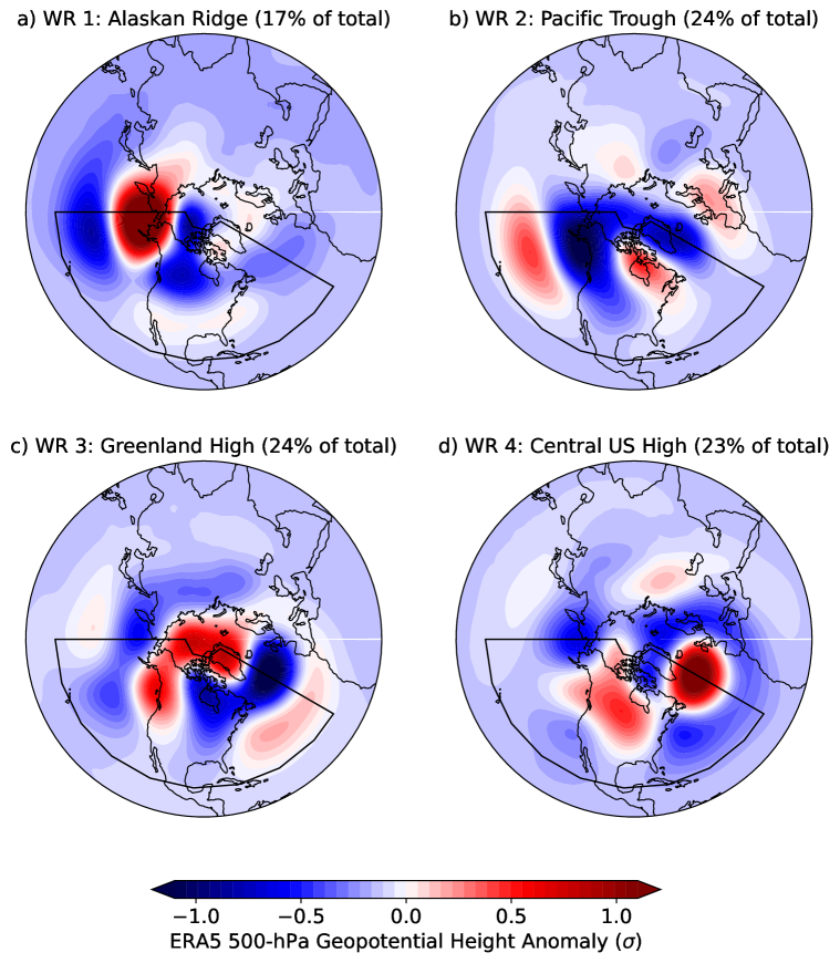
After obtaining the detrended standardized anomalies at a weekly temporal resolution, the methodology described by Molina et al. (2023a) and Lee et al. (2023) was replicated. First, we extracted the 12 leading principal components (PCs) from the weekly Z500 fields. Then, we identified the WRs by applying k-means clustering with four centroids over the time series of these 12 PCs (Michelangeli et al., 1995). Following Lee et al. (2023), we created a fifth class called “No WR,” which corresponds to samples that are closer to the origin than to any of the four WR centroids; that is, the PC scores are closer to the (0, 0, 0, … 0) point on the PC space. The average Z500 detrended anomalies associated with the four identified WR classes are shown in Figure 1. Consistent with nomenclature from past studies (e.g., Lee et al., 2019; Robertson et al., 2020; Molina et al., 2023a; Lee et al., 2023), the identified large-scale WRs were named Alaskan Ridge, Pacific Trough, Greenland High, and Central United States (US) High (Figure 1).
2.3 Sources of Predictability and Input Data for the Models
Disregarding external forcings, such as anthropogenic or volcanic emissions, the primary sources of S2S predictability can be classified into two categories: i) the state of recurring or quasi-oscillatory patterns, and ii) anomalies in the initial state of one of the components of the Earth system whose typical timescale of evolution (i.e., persistence time) is similar to the target forecast (National Academies of Sciences et al., 2016). In this study, we start from the (imperfect) assumption that most of the information corresponding to those two categories is contained within a limited set of variables from three Earth system components (ocean, land, and atmosphere). Additionally, we assume that the XGBoost models, in conjunction with a sufficiently large sample size, are skillful enough to at least partially represent the physical laws that determine the spatiotemporal behavior of the processes affecting the future state of the atmosphere within the S2S temporal horizon.
Each model within this study is trained separately using one variable from one of the three considered Earth system components. For the atmosphere and land, we used data from ERA5 and ERA5-Land (Muñoz-Sabater et al., 2021) reanalyses, respectively. For the ocean, we used data from the Simple Ocean Data Assimilation reanalysis (SODA; Carton et al., 2018). Taking into account various known sources of predictability originating from tropical and extratropical regions (e.g., Stan et al., 2017; Tseng et al., 2018; Lin et al., 2019), the spatial domain of all input variables span all longitudes (360∘ around the prime meridian) and latitudes from 30∘S to 90∘N. ERA5 and ERA5-Land datasets are available at a 0.1∘ horizontal grid spacing, while the SODA dataset is available at a 0.5∘ horizontal grid spacing. For the input variables to have a uniform but sufficiently detailed spatial resolution, all fields were re-gridded onto a 0.5∘ horizontal grid using nearest neighbor interpolation. In the following subsections, we describe the potential sources of predictability we aim to represent and the corresponding input variables.
All input variables were transformed into weekly detrended anomalies, following the steps described in Subsections 2.1 and 2.2. However, instead of removing the area average trend, each pixel was detrended separately. After obtaining the weekly detrended standardized anomalies by subtracting the daily climatology and dividing by the standard deviation, we performed a dimensionality reduction of the data by applying PC analysis, similar to what was done for WRs. For each variable, 20 leading PCs were used as XGBoost model inputs following a sensitivity assessment which found that skill did not change substantially with more PCs. Apart from the models trained separately with each variable to assess predictability from one individual variable, three other models were trained using atmosphere-only, land-only, or ocean-only variables as inputs. The same PC analysis was performed for dimensionality reduction, considering 20 PCs for each variable within the Earth system component.
2.3.1 Atmospheric variables
Four atmospheric variables were used in our study, with three from the troposphere and one from the stratosphere (Table 1). The variables from the troposphere are Z500, outgoing long-wave radiation (OLR), and 200-hPa zonal wind (U200). Z500 describes the mid-latitude atmosphere, including the large-scale atmospheric circulation (Cheng and Wallace, 1993), North-Atlantic oscillation (NAO; Wallace and Gutzler, 1981; Davini et al., 2012), planetary- and synoptic-scale waves (Blackmon, 1976), and blocking episodes (Tibaldi and Molteni, 1990; Scherrer et al., 2006). OLR provides information about the strength and spatial coverage of convective clusters, which are related to tropical-extratropical teleconnections (Stan et al., 2017), from the MJO (Hendon and Salby, 1994; Wheeler and Kiladis, 1999; Wheeler and Hendon, 2004), ENSO (Yulaeva and Wallace, 1994), and Indian Ocean dipole (IOD; Saji et al., 1999). U200 provides information about the shape and location of the polar and subtropical jet streams (Krishnamurti, 1961; Palmén, 1948; Strong and Davis, 2007), in addition to the coupling of the Walker circulation to the phase of ocean-related phenomena, like ENSO or IOD (Philander, 1983; Saji et al., 1999).
| \toplineVariable | Relevance to S2S forecasting |
|---|---|
| \midline500hPa geopotential height (Z500) | Mid-latitude atmosphere (e.g., weather regimes, North-Atlantic oscillation, |
| planetary Rossby waves, and blocking episodes). | |
| Outgoing longwave radiation (OLR) | Clusters of convection and large-scale cloud patterns. |
| 10hPa zonal wind (U10) | Quasi-biennal oscillation and sudden stratospheric warming events. |
| 200hPa zonal wind (U200) | Strength and structure of the walker cell, jet streams, and Indian Ocean dipole. |
| \botline |
The stratosphere is a valuable source of S2S predictability given its slowly varying circulation anomalies (National Academies of Sciences et al., 2016). During boreal winter, the stratosphere can interact with the upper troposphere and modify the tropospheric circulation, along with the onset and evolution of WRs (Baldwin and Dunkerton, 2001; Baldwin et al., 2003; Gerber et al., 2009; Domeisen et al., 2020). Two primary stratospheric mechanisms contributing to mid-latitude predictability have been previously identified, the quasi-biennial oscillation (QBO; Baldwin et al., 2001) and the stratospheric polar vortex (Gerber et al., 2009). The QBO is an easterly-to-westerly reversal of tropical stratospheric winds partly driven by waves originating from the troposphere that can affect the strength of the stratospheric polar vortex (Baldwin et al., 2001). Changes in the stratospheric polar vortex can result in large-scale tropospheric circulation anomalies with a lag of about one month (Thompson and Wallace, 2000; Baldwin and Dunkerton, 2001). Rapid slowdowns of the stratospheric polar vortex are frequently accompanied by sudden stratospheric warmings that can affect the Northern Annular Mode and contribute to an equatorward shift of the tropospheric midlatitude jet (Gerber et al., 2009; Domeisen et al., 2020). The zonal wind at 10-hPa (U10) is the fourth atmospheric variable we consider because it can help diagnose the QBO phase and the strength of the stratospheric polar vortex (Baldwin et al., 2001; Gerber et al., 2009).
2.3.2 Oceanic variables
The ocean is relevant for S2S prediction because it provides information about natural modes of climate variability and it can influence the overlying atmosphere (National Academies of Sciences et al., 2016). Perturbations of the ocean’s mean state, particularly within the tropics, can induce organized large-scale convection, modifying the heating distribution through the atmosphere and producing temperature and precipitation anomalies. Organized convection can also change the extratropical circulation due to propagation via Rossby wave-trains (Bjerknes, 1969; Horel and Wallace, 1981; Trenberth et al., 1998). ENSO is one of the primary modulators of long-lived tropical signals, with positive or negative SST anomalies over the eastern-to-central equatorial Pacific characterizing its warm and cold phases respectively (Philander, 1983).
The atmosphere can also respond to extratropical ocean features (Zhou, 2019), such as eddy-mediated processes, which can generate near-surface atmospheric baroclinicity and modify the spatial characteristics of overlying storm tracks (Kwon et al., 2010). Another example is a linear thermodynamic interaction, where geopotential heights are modulated above the ocean anomaly (Kushnir et al., 2002). Although the atmospheric variance associated with extratropical SST anomalies is modest compared to internal atmospheric variability, extratropical SST anomalies can persist for months to years (Chelton and Xie, 2010) and the atmosphere can respond within a few months (Ferreira and Frankignoul, 2005; Deser et al., 2007).
Ocean data was sourced from SODA reanalysis (Table 2). To capture information about subsurface conditions that may reach the surface via mixing (Alexander, 1992), we used ocean heat content (OHC) integrated from the surface to different depths (50m, 100m, 200m, 300m, and 700m). Sea surface height (SSH) and mixed layer depth (MLD) were also used, which provide information about the upper-ocean circulation, anomalous upwelling or downwelling, and the size, depth, and location of eddies (Chelton et al., 2011; Kurczyn et al., 2012; Uchoa et al., 2023).
| \toplineVariable | Relevance to S2S forecasting |
|---|---|
| \midlineSea surface temperature (SST) | ENSO, storage of anomalous surface heat, and eddies. |
| Ocean heat content (OHC) integrated from the surface | Magnitude and persistence of anomalous heat. |
| to a 50m, 100m, 200m, 300m, or 700m depth. | |
| Mixed-layer depth (MLD) | Anomalous upwelling or downwelling, and upper-ocean circulation structure. |
| Sea-surface height (SSH) | Anomalous upwelling or downwelling, and upper-ocean circulation structure. |
| Sea ice thickness (IT) | Anomalous changes of heat and moisture fluxes from the ocean to the atmosphere, |
| and changes in albedo. | |
| Sea ice concentration (IC) | Anomalous changes of heat and moisture fluxes from the ocean to the atmosphere, |
| and changes in albedo. | |
| \botline |
Sea ice thickness and concentration anomalies were also used, which are generally slow-evolving and describe sea ice cover (Table 2). Sea ice can significantly reduce heat and moisture fluxes from the ocean to the atmosphere, modifying the surface albedo and increasing how much incoming radiation is reflected (National Academies of Sciences et al., 2016). The presence and persistence of sea ice can also affect the paths of atmospheric lows (Balmaseda et al., 2010; Screen et al., 2011).
2.3.3 Land variables
Soil water content can influence surface energy budgets, contributing to anomalies in temperature and precipitation, and is therefore another source of S2S predictability (Koster et al., 2004, 2010; Guo et al., 2011; Koster and Walker, 2015; Roundy and Wood, 2015; Thomas et al., 2016). ERA5-Land, based on the Tiled ECMWF Scheme for Surface Exchanges over Land (TESSEL; Balsamo et al., 2009) and forced with ERA5 atmospheric fields, provides temperature and water content for four layers down to a depth of 2.89m. Soil water content (SWC) and soil temperature (ST) integrated from the surface to the depth of each one of the four reanalysis layers (7cm, 28cm, 1m, and 2.89m) are used as input variables (Table 3). Terrestrial snow is another source of S2S predictability given its radiative effects and liquid water that is released during melting (Peings et al., 2011; Jeong et al., 2013; Orsolini et al., 2013; Thomas et al., 2016). Thus, we used snow depth (SD) as an input variable for some land-only ML models.
| \toplineVariable | Relevance to S2S forecasting |
|---|---|
| \midlineSoil water content (SWC) integrated from the surface | Storage of surface water, and proxy for soil and |
| to a 7cm, 28cm, 1m, or 2.89m depth. | vegetation characteristics. |
| Soil temperature (STL) averaged from the surface | Proxy for potential evaporation and proxy for soil |
| to a 7cm, 28cm, 1m, or 2.89m depth. | and vegetation characteristics. |
| Snow depth (SD) | Storage of surface water and influence on surface energy budgets. |
| \botline |
2.4 XGBoost hyperparameters
We performed a Bayesian optimization (Snoek et al., 2012) of hyperparameters for each ML model to obtain the combinations that produced the best possible performance within the limits of our study. We emphasize that our objective is not to obtain the best possible S2S forecasts but to assess predictability contributions from different variables and Earth system components. Given the potential presence of certain states of modes of climate variability, a model may perform better when evaluated in one particular period than another. To prevent overfitting to such patterns, we used k-fold cross-validation to find the best combination of hyperparameters and cross-testing to obtain performance metrics representative of the whole study period. The “cross-validation and cross-testing” approach has been shown to remove biases when assessing performance while also taking advantage of all samples within the dataset (Korjus et al., 2016). The hyperparameter search is performed independently for each variable and lead time.
We employed cross-validation and cross-testing in the following manner for each one of the variables. The 40-year dataset was divided into four decades (1981-1990, 1991-2000, 2001-2010, and 2011-2020). For cross-testing, we denoted a test subset as one of the four decades. A model predicting a test subset was then trained using the remaining three decades of data. Before training on the remaining three decades, we applied three-fold cross-validation, where each one of the decades served as one “fold.” Three-fold cross-validation allowed us to obtain the combination of hyperparameters that provided good skill across each held out fold, which involved trying multiple combinations of hyperparameters and training iteratively on two of the three decades. Finally, the combination of hyperparameters yielding the best average performance over the three decades was chosen to predict the respective test subset, and this process was repeated three more times to obtain performance statistics on the four test subsets.
Ten hyperparameters were assessed during optimization (Table 4), including those related to the complexity of the trees (e.g., maximum tree depth) and to prevent overfitting (e.g., L1 and L2 regularization terms). Additionally, we assessed the impact of adding class weights to control for WR class imbalance. The Bayesian algorithm (Snoek et al., 2012) used to perform the hyperparameter search approximates a probabilistic function to the hyperparameter field to make iterative changes in a direction that improves the objective function. We used the F1 score as the objective function, which is similar to “threat score” and “critical success index,” and focuses on the fraction of observed and forecast events that were correctly predicted. The advantage of the F1 score over other objectives, such as accuracy, lies in that it neglects “true negative” cases that can artificially inflate skill when a class imbalance exists. 50 initial trials with random hyperparameter combinations were run to provide an initial performance baseline and then 50 subsequent iterations were performed using the Bayesian algorithm to find the best combination. For the hyperparameter optimization stage, 100 estimators (trees or boosting rounds within the XGBoost algorithm) were used for each model. After finding the best set of hyperparameters, 300 estimators (i.e., the number of boosting rounds or trees) were used to train the final XGBoost model for each variable or combination of variables. Table 4 shows the optimal hyperparameters identified during the search.
| \toplineHyperparameter | Search range | Optimal values |
| \midlineMaximum depth of a tree | 3-12 | 9-12 |
| Minimum sum of instance weight needed in a child | 1-50 | 30-40 |
| Percentage of samples used for each tree construction | 0.1-1 | 0.8-1 |
| Percentage of features used for each tree construction | 0.1-1 | 0-0.25 |
| Percentage of features used for each split | 0.1-1 | 0.8-1 |
| Learning rate | 0.01-0.3 | 0.25-0.3 |
| Minimum loss reduction required to make a further partition on a leaf node of a tree (gamma) | 0-3 | 0-0.5 |
| L1 regularization term on weights | 0-10 | 0-2 |
| L2 regularization term on weights | 0-10 | 0-2 |
| Weighted loss for class imbalance | Boolean | True |
| \botline |
3 Results
3.1 Sources of predictability based on ML model skill
Plots a, b, and c in Figure 2 show the F1 score as a function of lead time for each ML model trained using atmospheric, oceanic, or land predictors. For the atmosphere-only models (Figure 2a), predictability from certain predictors is higher during earlier lead times. For example, during weeks 1-2, the models using Z500 or U200 as predictors perform better than models using OLR or U10. A model trained using all atmosphere predictors performs well during weeks 1-3 and exceeds the performance of the other models during weeks 5-7. Some variables provide more predictability later in the forecast horizon. For instance, U10 provides predictability during weeks 5-7, indicating lagged contributions via the QBO and stratospheric polar vortex (Baldwin et al., 2001; Gerber et al., 2009). OLR provides predictability during week 8, indicating the importance of tropical-to-extratropical teleconnections during the later forecast horizon.
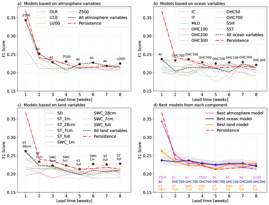
ML models trained using ocean predictors exhibit consistent spread in performance across lead times (Figure 2b). OHC integrated to different depths, particularly 700m, appears as the best predictor for most lead times except week 1 when the all-variables model provides the highest predictability. Predictability from SSH, which is moderate across lead times, is likely related to the thermal state of the tropical ocean, gyres, and other extra-tropical oceanic features. Comparably less predictability is offered by ice thickness and ice concentration, possibly due to seasonality. Limited predictability from SST as a predictor supports the need to account for the subsurface in addition to surface conditions.
The performance of ML models trained with land predictors exhibits less spread from week to week compared to ocean predictors making it difficult to rank land predictor importance; however, some predictors stand out (Figure 2c). For example, ST in the most superficial layers provides more predictability for weeks 1-2. After week 3, ST and SWC integrated into the deepest layers provide more predictability across most lead times. These results suggest that land-based S2S predictability mainly comes from evaporative processes, highlighting the importance of continuing to improve the coverage of soil in situ observations (e.g., Hasan et al., 2020).
Figure 2d compares the best-performing ML models based on the F1-score from each Earth system component. Results indicate that the atmosphere provides comparatively greater predictability at 1-2 week lead times. Ocean-based predictability outperforms the other components during weeks 3 and 6 (although within confidence levels). Land-based predictability increases during later lead times, outperforming the other components at week 8, though also within the envelope spread. All Earth system components outperform persistence during later lead times. We also note that predictability was not necessarily improved when using all predictors from the respective Earth system component, potentially due to competing predictive signals or limitations associated with partially correlated predictors (Figure 2a-c).
3.2 Seasonality of the sources of predictability
Given the seasonality of the midlatitudes, certain predictors may provide more predictability during certain periods of the year. Some examples include seasonal variations of land heat and moisture fluxes, incident radiation and radiative fluxes, and sea ice thickness and extent. Figure 3 shows predictability stratified by season and notable seasonal differences are found.
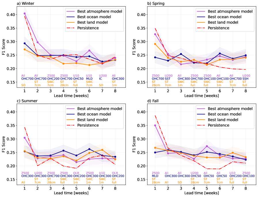
During winter (Figure 3a), the best-performing atmosphere-only models offer more predictability than other components during the first two weeks. The importance of stratospheric dynamics in S2S predictability during boreal winter is also elucidated; Z500 is the best predictor during weeks 3-4, and U10 is best at weeks 5-6. Ocean-based predictability decreases gradually across the forecast horizon, with OHC being the best predictor until week 5. Land-based predictability decreases throughout the forecast horizon, with small increases during weeks 7-8. The importance of snow depth (SD) as a predictor at weeks 1 and 7 is also evident during winter.
During spring (Figure 3b), the atmosphere provides more predictability during weeks 1-2, oceanic-based predictability is higher during week 3, and land-based predictability is higher during week 4, although with overlapping confidence bounds. SWC is also important during weeks 3-6, which is in agreement with studies finding that soil water content offers more predictability before summer when land-surface energy transfers become active (Conil et al., 2009; Guo et al., 2012; Thomas et al., 2016). Predictability from all components increases during later lead times, suggesting influence from boundary conditions or lagged processes in spring (Meehl et al., 2021).
Predictability from the atmosphere is lower during summer at early lead times (Figure 3c), which is expected because of the reduced influence of the jet stream and associated large-scale circulation. Predictability from the ocean is higher during summer, particularly during week 6. Similar to spring, land-based predictability decreases until week 5 and then increases, likely due to information contained in soil water content. The best-scoring predictors during most lead times were OHC and SWC for the ocean and land, respectively.
During fall (Figure 3d), higher predictability is evident from the atmosphere during weeks 1 and 5 relative to the other components, similar to winter. Land-based models show the highest skill during weeks 7 and 8, and ocean-based models show the highest skill during weeks 2, 3, 4, and 6, within confidence intervals.
Although not the focus of our study, predictability from all components exceeds persistence at weeks 3-8 during spring, summer, and fall. Persistence exhibits more predictability during winter, illustrating that baselines can complicate ML model assessments if seasonality is not considered.
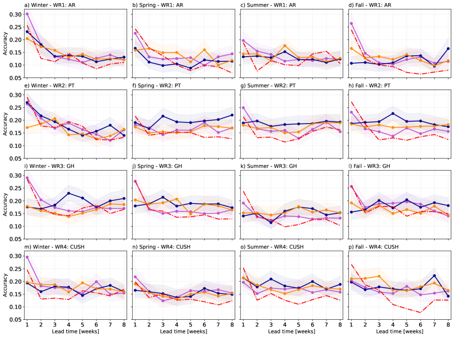
3.3 Variations in predictability sources based on WR
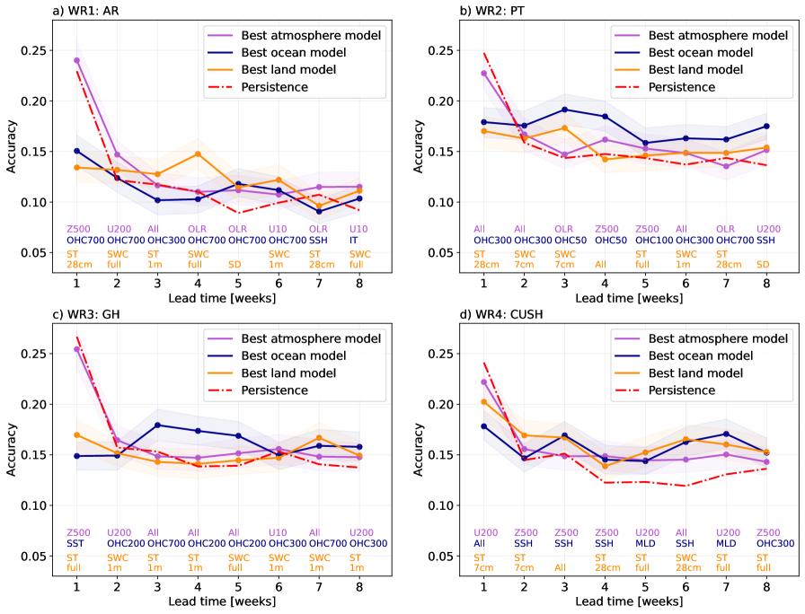
Different WRs may have differing sources of predictability. Figure 4 shows the accuracy of the best-performing ML models from each component as a function of lead time and stratified by WR, and Figure 5 is further stratified by season. Additionally, Tables 5-7 show the corresponding predictors that the best models are based on.
| \topline | 1 | 2 | 3 | 4 | 5 | 6 | 7 | 8 | |
|---|---|---|---|---|---|---|---|---|---|
| WR | Season | ||||||||
| \midlineAR | Winter | Z500 | ALL | ALL | ALL | OLR | U200 | U200 | U10 |
| Spring | ALL | ALL | Z500 | OLR | U10 | OLR | OLR | U10 | |
| Summer | Z500 | U200 | OLR | ALL | OLR | OLR | ALL | U10 | |
| Fall | ALL | ALL | U200 | Z500 | U200 | U200 | U10 | ALL | |
| PT | Winter | ALL | ALL | Z500 | Z500 | Z500 | U10 | Z500 | Z500 |
| Spring | OLR | U200 | OLR | Z500 | Z500 | ALL | U200 | U200 | |
| Summer | ALL | U200 | OLR | Z500 | U10 | Z500 | Z500 | U200 | |
| Fall | Z500 | Z500 | U10 | Z500 | Z500 | U10 | OLR | Z500 | |
| GH | Winter | Z500 | U200 | Z500 | ALL | U10 | U10 | ALL | U200 |
| Spring | Z500 | U200 | ALL | ALL | OLR | ALL | U200 | U200 | |
| Summer | Z500 | ALL | U10 | Z500 | ALL | Z500 | U10 | OLR | |
| Fall | U200 | ALL | ALL | U10 | ALL | U10 | ALL | OLR | |
| CUSH | Winter | ALL | ALL | U200 | Z500 | U200 | U10 | ALL | ALL |
| Spring | U200 | U200 | U200 | U200 | U10 | ALL | U200 | U200 | |
| Summer | U200 | Z500 | Z500 | Z500 | OLR | Z500 | U10 | OLR | |
| Fall | U200 | Z500 | ALL | OLR | U200 | OLR | U200 | Z500 | |
| \botline |
| \topline | 1 | 2 | 3 | 4 | 5 | 6 | 7 | 8 | |
|---|---|---|---|---|---|---|---|---|---|
| WR | Season | ||||||||
| \midlineAR | Winter | OHC700 | OHC700 | OHC300 | OHC700 | SSH | OHC700 | OHC50 | OHC700 |
| Spring | OHC700 | OHC700 | SST | SSH | MLD | SST | MLD | MLD | |
| Summer | IT | OHC50 | OHC300 | OHC100 | OHC700 | OHC300 | OHC700 | OHC700 | |
| Fall | OHC700 | OHC300 | OHC700 | OHC700 | OHC700 | OHC700 | IT | IT | |
| PT | Winter | OHC700 | SST | OHC50 | IT | IT | OHC300 | SST | OHC300 |
| Spring | OHC50 | SST | OHC50 | OHC700 | ALL | SSH | OHC700 | SSH | |
| Summer | OHC300 | OHC300 | OHC50 | OHC50 | OHC100 | OHC300 | ALL | OHC700 | |
| Fall | MLD | OHC300 | OHC300 | OHC50 | OHC50 | OHC100 | ALL | MLD | |
| GH | Winter | OHC700 | OHC700 | OHC200 | OHC200 | OHC50 | OHC700 | OHC700 | OHC700 |
| Spring | OHC700 | ALL | OHC700 | OHC100 | OHC200 | OHC100 | OHC700 | OHC700 | |
| Summer | OHC300 | OHC200 | MLD | OHC300 | SSH | SST | SSH | OHC300 | |
| Fall | OHC700 | OHC300 | OHC700 | OHC200 | SSH | OHC50 | OHC300 | OHC200 | |
| CUSH | Winter | ALL | SSH | OHC200 | SSH | SSH | MLD | MLD | OHC300 |
| Spring | SSH | SST | OHC200 | OHC200 | OHC100 | OHC100 | SSH | OHC300 | |
| Summer | ALL | OHC700 | OHC700 | OHC100 | OHC200 | IC | IC | SST | |
| Fall | MLD | OHC200 | SSH | OHC100 | MLD | MLD | MLD | OHC200 | |
| \botline |
| \topline | 1 | 2 | 3 | 4 | 5 | 6 | 7 | 8 | |
|---|---|---|---|---|---|---|---|---|---|
| WR | Season | ||||||||
| \midlineAR | Winter | ALL | ST 28cm | ST 7cm | SD | ST 1m | ST 7cm | ST 28cm | SWC full |
| Spring | ST 28cm | ST 7cm | ST 1m | SWC full | SWC full | SWC 1m | SWC 1m | SWC 1m | |
| Summer | SWC full | SWC full | ST 1m | SWC full | SD | SWC 1m | SWC 28cm | SWC full | |
| Fall | ALL | ST full | SWC full | SWC full | SWC full | ST full | ST 28cm | ST 1m | |
| PT | Winter | SWC full | SWC 7cm | SWC 7cm | ALL | ST 1m | SWC 1m | SD | SD |
| Spring | ST 28cm | ALL | SWC full | SWC 1m | ST 7cm | ST 1m | ST 7cm | ST full | |
| Summer | ALL | SWC 7cm | SWC 7cm | ST 7cm | ST full | SWC 1m | SWC 1m | SWC 28cm | |
| Fall | SWC full | SWC full | SWC 7cm | SWC 7cm | ST full | ST 7cm | ST 28cm | ST 7cm | |
| GH | Winter | SD | SD | SD | SD | SD | SWC 28cm | SWC 1m | SWC 1m |
| Spring | ST 1m | SWC 28cm | ST full | SWC 7cm | SWC 1m | SD | SWC 1m | ST 1m | |
| Summer | ST full | SWC 1m | ST 28cm | ST 1m | ST 1m | SWC 1m | SWC 1m | ST full | |
| Fall | SWC 7cm | ST 1m | ST 1m | ST 28cm | SWC full | ST 7cm | ST full | ST 28cm | |
| CUSH | Winter | ST 7cm | ST full | ST full | ST full | ST full | ST full | ST full | ST full |
| Spring | ST 28cm | ST 7cm | ST 28cm | SWC full | SD | SWC 28cm | ST 1m | ST 7cm | |
| Summer | ST 7cm | ST 7cm | ALL | SWC full | SWC 1m | SWC 28cm | SWC 1m | ST full | |
| Fall | ST 7cm | ST 1m | ST 28cm | ST 1m | ST full | SWC 28cm | SWC 28cm | ALL | |
| \botline |
3.3.1 Alaskan Ridge
For the Alaskan Ridge regime (Figure 4a), atmosphere-based models showed the most accuracy during weeks 1-2 and 7-8, with the latter related to OLR and U10 contributions. Ocean-based models were best during week 5 (though within confidence bounds), largely associated with OHC. Land-based models were best during weeks 3, 4, and 6, associated with SWC and ST. Notable seasonal differences in accuracy were also found. During winter (Fig. 5a), atmosphere-based models performed best during weeks 1-2 and 6-7, with the latter associated with U200. ST outperformed the other variables during weeks 3 and 5, and OHC provided more predictability during weeks 4 and 8 (within confidence bounds). In spring, land-based models performed best during weeks 2-4 and 6, while atmospheric models performed best during weeks 1, 5, 7, and 8 (Fig. 5b). For land-based models, ST contributed more predictability during earlier lead times and SWC during later lead times (Table 7). OLR and U10 frequently appeared as the best atmospheric predictors (Table 5). In summer (Figure 5c), the atmosphere is the best predictor during earlier lead times and land is better in later weeks. The best atmospheric predictors are mixed, while land predictability is largely associated with SWC (Table 7). During fall (Figure 5d), atmospheric models are more accurate during weeks 1, 2, and 7, land-based models perform best during weeks 3-5, and ocean-based models perform best during weeks 6 and 8; U10, SWC, OHC, and ice thickness (IT) were the best predictors (Tables 5-7).
3.3.2 Pacific Trough
Ocean-based models performed most accurately when predicting the Pacific Trough regime starting at week 2 lead time, with predictability largely from OHC (Figure 4b). Seasonal stratification shows that predictability from the ocean for the Pacific Trough regime is consistent year-round (Figure 5e-h). During winter (Figure 5e), the best ocean predictors are mixed, but Z500 is the best atmospheric predictor during most lead times, while SWC and snow depth (SD) are the best land predictors (Tables 5-7). Ocean-based model accuracy increases during spring, largely associated with OHC (Table 6), while the atmosphere- and land-based accuracy remains nearly constant as a function of lead time (Figure 5f). Predictability during summer is similar to spring except for land-based predictability, which increases in later lead times due to contributions from SWC (Figure 5g, Table 7). During fall OHC is still most accurate during most lead times (Figure 5h).
3.3.3 Greenland High
Most predictability comes from the atmosphere when predicting the Greenland High regime at lead times of 1-2 weeks (Z500 and U200), and then the ocean provides more predictive skill until week 5 (OHC; Figure 4c). The land contributes more predictability at week 7, related to SWC. Stratifying by season further corroborates that the ocean is a dominant source of predictability after week 2 during winter, spring, and fall, largely related to OHC (Figure 5i,j,l, Table 6). The land also exhibits higher predictability after a lead time of 2 weeks during spring and summer. Although not the best predictor overall, snow depth (SD) appears as the best land predictor during some winter and spring lead times (Table 7), illustrating the importance of snow for predicting the Greenland High regime (Figure 5i-j). In addition to SWC, ST is an important source of land-based predictability during summer and fall (Table 7). U10 appears repeatedly as the best atmospheric predictor during most subseasonal lead times (i.e., week 3+) in summer, fall, and winter (Table 5).
3.3.4 Central-US High
The three Earth system components exhibit similar accuracy in predicting the Central US High regime, with improvement in land- and ocean-based performance after week 5 (Figure 4d). The jet stream (i.e., U200), SSH, and ST contribute skill most frequently across the forecast horizon (Tables 5-7). Predictability differences between Earth system components become more evident during certain seasons. In summer, the ocean contributes the most predictability, associated with OHC, IC, and SST (Table 6). During Fall, land-based models perform better, particularly during earlier lead times. Similar to other WRs, ST is the best predictor during earlier lead times while SWC is best during later weeks. During winter and spring, the accuracy among components exhibits a lot of overlap. The variables that offer the highest accuracy during winter are U10, SSH, MLD, OHC, and ST. The best predictor during spring for the Central-US High regime at most lead times is U200.
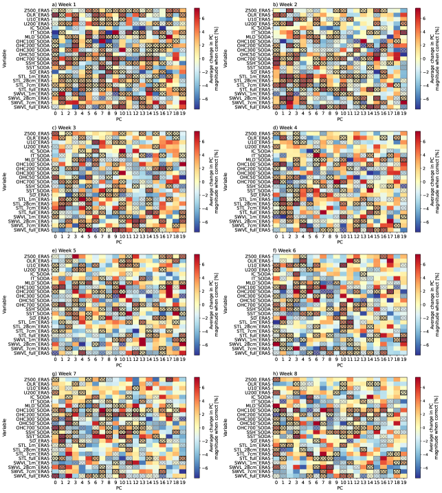
3.4 Physical processes contributing predictability
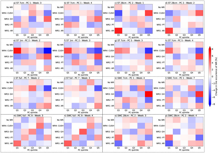
In this section, we explore processes that contribute to the predictability of WRs and describe some of their main characteristics. Although the spatial dimensionality of predictors was reduced using PC analysis, the spatial fields of leading PCs can be reconstructed for interpretation. Recall that 20 leading PCs were used per predictor as input features into XGBoost. Here we focus on the PCs that are meaningfully associated with a change in the future likelihood of a WR occurring. To identify these PCs, the heatmaps in Figure 6 were constructed using
| (1) |
where D is the respective PC scores (absolute values) of all samples, n is the total number of D samples, a is a subset of the respective PC scores from D when associated WR predictions are correct, and na is the number of a samples. In other words, the heatmap shows the percent change between the average PC score magnitudes when predictions are correct and the average PC score magnitudes for all predictions. A larger percent change indicates that the respective PC is on average more anomalous when it results in a correct prediction. Additionally, a chi-squared test of independence was used to assess whether large PC scores, defined as greater than the 80th percentile of scores or less than the 20th percentile of scores, are associated with a statistically significant change in the distribution of WRs at the specific lead time considered as compared to WR climatology. The null hypothesis states that the change in WR distribution at a specific lead time happened by chance. Grey hatching in Figure 6 indicates PCs and variables where the null hypothesis was rejected (=0.05) stratified by lead time. Lastly, black hatching was used if, in addition to grey hatching, the mean of the absolute values of scores associated with correct WR predictions was greater than the mean of the absolute values of all scores. The processes associated with black hatched PCs will be considered ‘relevant’ and of focus for the rest of the manuscript because they are associated with a meaningful change in WR distribution and correct WR forecasts.
3.4.1 Atmospheric precursors
Figure 6 shows that several atmospheric processes contribute to WR predictability. For 500-hPa geopotential height anomalies, PCs 0, 2, 9, and 10 appeared as relevant after week 1. Figure 7 shows the spatial patterns (i.e., Empirical Orthogonal Function or EOFs) associated with the positive phase of PC0 and PC2. Since PC9 and PC10 explain less than 2% of Z500 variance, we focus on PC0 and PC2, although we note that EOF9 and EOF10 indicate Rossby wave trains in the mid-latitudes (not shown). The PC0 time series exhibits multi-year variability and its EOF shows high variance over the tropics, likely associated with ENSO (Fig. 7a and Fig. 8a). PC0 is related to an increased likelihood of the Greenland High regime (weeks 4 and 8) and a decrease of the Pacific Trough regime (week 8) when it is in a positive phase (Q5 in Fig. 9a,b). EOF2 manifests as a wavenumber-2 pattern over the high latitudes and the WRs likelihood response is asymmetric between upper and lower quintiles of WR likelihood: when the PC scores are below the 20th percentile (Q1), there is an increase in the likelihood of the Central-US High regime and a decrease in the likelihood of the Alaskan Ridge regime during weeks 2 and 3 (Fig. 9c,d), but the opposite signal is weaker when the PC scores are higher than the 80th percentile (Q5).
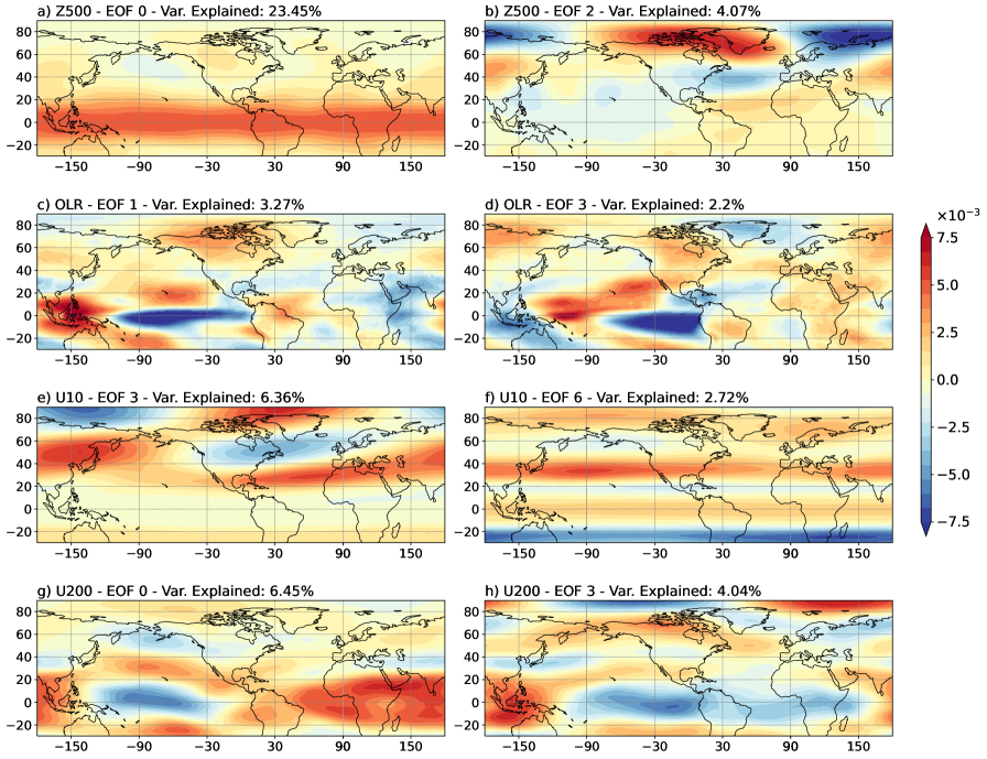
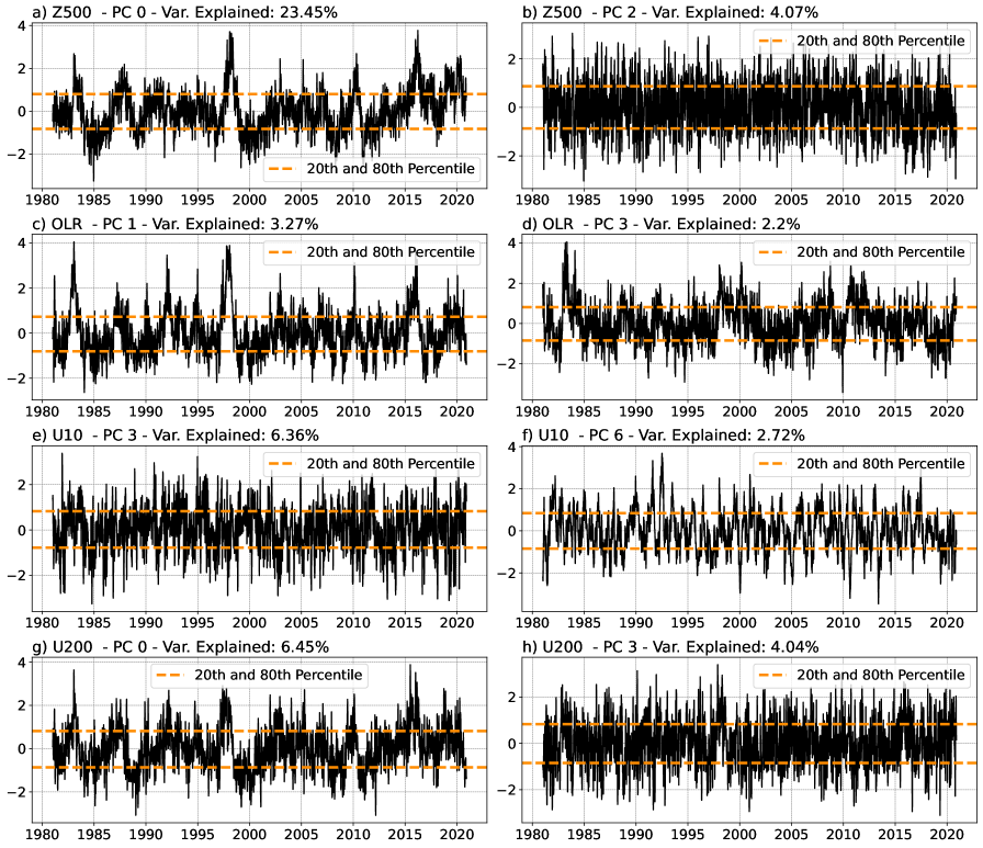
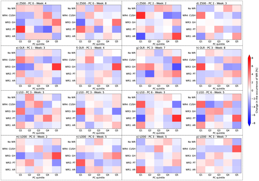
For OLR, PCs 1, 3, 10, and 18 appeared as relevant at lead times beyond week 1 (Figure 6). Since PC10 and PC18 explain less than 2% of OLR variance, we focus on PC1 and PC3. EOF1 is associated with high variance over the central tropical Pacific Ocean and Maritime Continent (Fig. 7c). Like the PC0 time series for Z500, PC1 for OLR is associated with an increased likelihood of the Greenland High regime during weeks 2 to 5, likely related to ENSO variability (Fig. 8c and Q5 in Fig. 9e,f)). EOF3 shows high variance over the Maritime Continent and the eastern tropical Pacific, with a variance of the opposite sign over the central tropical Pacific that extends to the West Coast of the US (Fig. 7d). EOF3 may be ENSO (warm phase) and/or MJO driven (phases 4, 5, and 6). PC3 is associated with shifts in the likelihood of the Pacific Trough and Greenland High regimes during the late stages of the forecast (weeks 7 and 8; Fig. 9g,h).
The most relevant PCs for U10 are PC3, PC6, and PC10 (Figure 6). PC10 has a variance explained of less than 2%, therefore we focus on PC3 and PC6. EOF3 exhibits high U10 variance from the Gulf of Mexico to Asia, over the Arctic proximal to Greenland, and a high variance of the opposite sign over North America, the North Atlantic, and the Arctic proximal to Siberia (Fig. 7e). EOF3 is physically associated with stratospheric zonal convergence over the Northeastern extra-tropical Pacific and divergence to the north, over the Arctic Ocean (Fig. 7e). The negative PC scores associated with this pattern are related to an increase in the likelihood of the Greenland High regime during weeks 3 to 5 (Q1 in Fig. 9i,j). EOF6 illustrates high U10 variance in the subtropics and polar regions (Fig. 7f). The negative phase of EOF6 may be related to sudden stratospheric warmings since the polar stratospheric jet would slow during such events. EOF6 is associated with an increase in the likelihood of the Pacific Trough regime and a decrease in the likelihood of the Central-US High regime during weeks 1 to 5 (Q5 in Fig. 9k,l).
Relevant PCs for U200 are 0, 3, and 15 (Fig. 6), with PC10 explaining less than 2% of the variance of U200, so focus is placed on PCs 0 and 3. EOF0 exhibits high variance over the tropics of opposite signs over the Atlantic and Pacific equatorial waters, likely related to modulations of the Walker circulation and ENSO (Fig. 7g). The positive phase of EOF0 relates to the likelihood of the Pacific Trough regime, which decreases in frequency from weeks 2 to 5 (Q5 in Fig. 9m,n). In contrast, the likelihood of the Greenland High regime increases at a week 2 lead time. EOF3 also shows high variance over the tropical Pacific, but with a shorter time scale of variability as compared to PC0 (Fig. 7h, Fig. 8h). PC3 is related to an increase in the likelihood of the Central-US High regime near the end of the forecast horizon (Q5, week 7), and negative PC scores are associated with an increase in the likelihood of the Alaskan Ridge regime at week 5 (Q1 in Fig. 9o,p).
3.4.2 Oceanic precursors
Numerous oceanic processes and climate modes of variability relevant to S2S predictability (e.g., ENSO) were consistently found to contribute to WR predictability (Figure 6). PC0 for OHC integrated to 700m, OHC integrated to 300m, and SSH all are relevant for WR prediction and all resemble ENSO in their EOF0 patterns and PC time series (Figs. 10a and 11a). The influence of ENSO is still reflected in these fields even though the predictors contain information well below the surface. Additionally, the high variance across the Indian Ocean resembles the IOD, which is related to ENSO (Ashok et al., 2001). The negative phase of these predictors (La Niña-like) is associated with an increase in the likelihood of the Pacific Trough regime across all lead times, in contrast to a decrease in the likelihood of the Greenland High regime (Q1 in Fig. 12a,b). EOF3 for OHC integrated to 50m shows an ENSO-like pattern and its PC time series also makes clear that the Pacific Decadal Oscillation (PDO; Mantua and Hare, 2002) is imprinted on the respective PC (Figs. 10b and 11b). The more slowly evolving mode of variability does not show a clear relationship with WR likelihoods (Fig. 12c,d), although there is a decrease in the likelihood of the Greenland High regime when PC scores are above the 80th percentile (Q5). EOF2 for SSH and its PC time series resemble ENSO, but with high variance across the equatorial Pacific shifted farther west, potentially related to a different flavor of ENSO and build-up of the warm pool (Fig. 10c). This pattern is associated with a higher likelihood of occurrence for the Pacific Trough regime through week 5 (Q5 in Fig. 12e,f). EOF3 for OHC integrated to 100m and 700m are relevant for predicting WRs but are more difficult to interpret. Both show a dipole-like variance pattern across the central and southern Pacific, but their association with WRs is mixed (Fig. 12g,h).
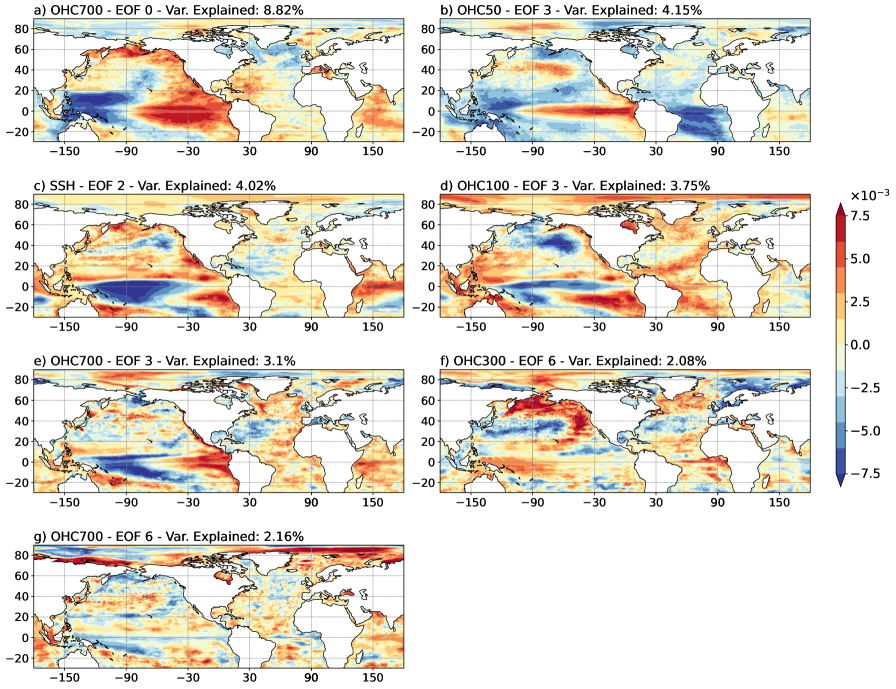
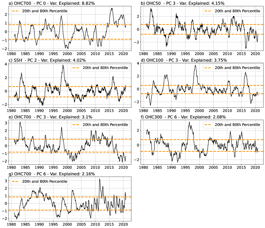
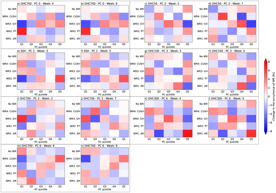
Some oceanic predictors display an influence from the North Pacific gyre. For example, EOF6 of OHC integrated to 300m shows high variance across the North Pacific, with a dipole-like pattern between the coasts of the Pacific Northwest and the central-to-western Pacific (Fig. 10f). This pattern is associated with an increased likelihood of the Alaskan Ridge regime occurring from week 4 onwards (Q5 in Fig. 12k,l). Other oceanic processes with more slowly evolving variability outside the tropical Pacific Ocean are indicated by EOF6 of OHC integrated to 700m (and 100m, although not shown) where there is a high variance over the Indian Ocean and a high variance dipole pattern (of opposite signs) over the Arctic Ocean (Figs. 10g). The negative PC scores from both of these predictors are associated with a decrease in the likelihood of the Central-US High regime (Q1), while the response to the positive phase (Q5) is the opposite but weaker (Fig. 12m,n).
3.4.3 Land precursors
Numerous land processes contribute to WR predictability, including ST and SWC (Fig. 6). We again focus on the PCs containing more than 2% variance explained. EOF1 for ST integrated to 7cm (and 28cm, though not shown due to similarities) shows high variance over the Amazon, Sub-Saharan Africa, and Asia (Fig. 13a); associated with increases in the likelihood of the Greenland High regime from weeks 2 to 4 (Q5 in Fig. 15a,b). EOF1 for ST integrated to 7cm also shows a high variance over Greenland and a high variance of the opposite sign over Europe (Fig. 13a). EOF2 for ST integrated to 28cm is related to high variance from Saharan Africa to Asia, and over Greenland, with high variance of the opposite sign over the Amazon, Sub-Saharan Africa, and Europe (Fig. 13); associated with an increased likelihood of the Central-US High regime and a decreased likelihood of the Alaskan Ridge regime during weeks 1 and 2 (Q5 in Fig. 15c,d). EOF2 for ST integrated to 1m shows a high variance over North America and Eastern Europe, and a high variance of the opposite sign over Australia, Western Europe, and Alaska; associated with a decrease in the likelihood of the Central-US High regime during weeks 2 and 3 (Q5 in Fig. 15e,f). The PC2 scores for ST integrated to 1m also increase during later years, suggesting the influence of a multi-decadal mode of climate variability or external forcing (Fig. 14c). EOF5 for ST integrated to 7cm shows a high variance over the Americas, Greenland, and the western Mediterranean, with a high variance of the opposite sign over northern Asia, Australia, and central-to-eastern Saharan Africa (Fig. 13d). The high-frequency variability of the PC5 time series for ST integrated to 7cm also shows an association with a decreased likelihood of the Central US High regime and an increased likelihood of the Greenland High regime during weeks 3-4 lead times (Q5 in Fig. 15g,h). EOF7 for ST integrated across all layers shows high variance across Greenland, South America, and Eastern Europe and its associated PC time series exhibits a slower mode of variability (Figs. 13e and 14e). This pattern is related to a decreased likelihood of the Central-US High regime during weeks 2-3 lead times (Q5 in Fig. 15i,j).
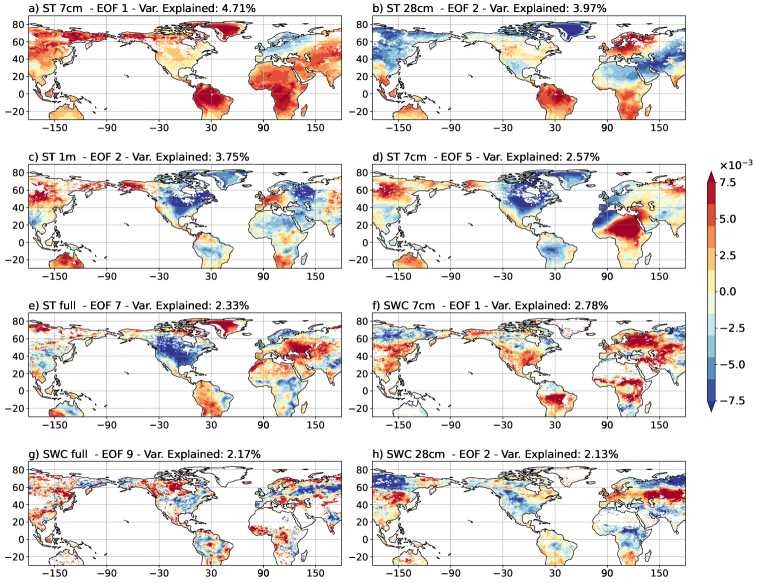
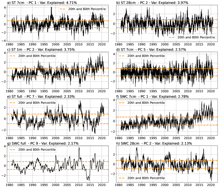
SWC PCs generally entailed less variance explained as ST PCs, but several were still identified as relevant and with variance explained greater than 2%. The PC time series for SWC integrated to 7cm was similar to that of PC2 for ST integrated to 1m; the influence of a multi-decadal mode of climate variability or external forcing is likely across the study period (Fig. 14f). EOF1 for SWC integrated to 7cm shows a high variance over the US, Amazon, eastern Europe, and Asia, with a high variance of the opposite sign over Siberia and Canada; a pattern strongly associated with likelihoods of the Greenland High and Pacific Trough regimes (Fig. 13f and Q5 in Fig. 15k,l). EOF9 for SWC integrated across the full available soil depth shows a heterogeneous pattern much noisier and more difficult to decipher than past patterns identified (Fig. 13g). PC9 time series for SWC integrated across the full-depth varies more slowly and results are mixed in terms of association with changes in the likelihood of WRs, except for the Alaskan Ridge regime, which shows an increase in the likelihood when PC9 is negative (Q1 in Figs. 15m,n). EOF2 for SWC integrated to 28cm shows high variance over the continental US. Variance is also high but with latitudinal stratification across Eurasia. These spatial patterns are associated with opposite sign changes in the likelihood of the Pacific Trough and Alaskan Ridge regimes for weeks 3 and 4 (Q1 and Q5 in Fig. 15o,p).
4 Conclusions
In this manuscript, we used ML to learn more about the sources of predictability of WRs over North America at S2S lead times. We trained several XGBoost models with an input variable from one of three Earth system components to assess their relative importance at various lead times and seasons. As expected, we found that atmospheric variables were better predictors during weeks 1-2 of the forecast. As lead time increases, the atmosphere, land, and ocean components contribute varying levels of predictability. For the atmosphere, the models using all variables as input features (OLR, U200, Z500, and U10) were frequently the best performers across several lead times. Ocean-based predictability came from ocean heat content, while soil water content and temperature mattered more for land-based predictability. ML models that included all variables from the land or ocean did not necessarily present the best skill, possibly due to competing predictive signals or limitations with using correlated variables. Thus, while convenient, it is not advisable to train an ML model that includes all predictors without special treatment or weighting. Contrary to our expectations, fewer variables could provide more predictability when using ML, particularly for slower-evolving land and ocean processes.
Our results also show how highly seasonally-dependent the sources of predictability are. Atmospheric-based predictability is more relevant during winter, while ocean-based is more so during summer. Predictability from land generally increases during later lead times in spring and summer. Sources of predictability were also dependent on the WR being predicted. Predictability from the ocean was higher than the land or atmosphere for the Pacific Trough and Greenland High regimes. Predictability from the land was comparably higher than the other components when predicting the Alaskan Ridge regime, although it was an overall less predictable regime than others. Central US High regime predictability also varied seasonally, where land contributed more predictability during fall and winter and the ocean contributed more during summer. Regarding specific predictors, ocean heat content was commonly the best predictor across seasons and regimes. Soil temperature and water content were also frequently relevant. Although atmospheric predictability was limited during later lead times, OLR frequently appeared relevant during spring and U10 during fall.
Relationships between predictors and the likelihood of WRs occurring were also explored across the forecast horizon. EOFs and PC time series showed an association between ENSO and the occurrence of the Pacific Trough and Greenland High regimes across subseasonal lead times, with La Niña-like conditions having a stronger impact on WR likelihoods, and therefore being a state of higher WR predictability. This association was stronger for OHC than SSTs, illustrating that the subsurface ocean enhances predictability. Convection (i.e., OLR) over the tropics and stratospheric winds (i.e., U10) were also relevant at subseasonal lead times, likely concerning the MJO and QBO. The North Pacific Gyre, IOD, and PDO were also reflected in ocean EOFs, and related to the occurrence of different WRs. SWC exhibited higher heterogeneity in EOF patterns than ST EOFs. Slower modes of climate variability, such as at multi-decadal scales, were also evident in the land PC time series.
Future work should focus on more deeply understanding sources of WR predictability, including testing causal hypotheses and quantifying how they may change in a warming climate. This study could also be expanded to incorporate other Earth system components and processes or delve further into the predictors herein. For example, we focused on explaining PCs with greater variance explained due to the large number of variables in our study, but some PCs with low variance were also associated with a statistically significant shift in WR occurrence. PC analysis is also limited to capturing linear signals, which may obfuscate nonlinear predictability in the Earth system. Our study is subject to limitations associated with clustering methods, wherein the WRs may be sensitive to the length of the observational record; a limitation that future work should also explore. Combined with domain knowledge, ML continues to present opportunities to elucidate sources of predictability.
Acknowledgements.
JSPC and MJM were supported by a University of Maryland Grand Challenges Seed Grant. Computing and data storage resources were provided by the Computational and Information Systems Laboratory at the National Science Foundation (NSF) National Center for Atmospheric Research (NCAR), which is a major facility sponsored by the NSF under Cooperative Agreement No. 1852977. The authors acknowledge the use of OpenAI’s ChatGPT for assistance in developing and refining the code used for analysis and visualization. \datastatementERA5 and SODA reanalyses can be obtained from the NSF NCAR Research Data Archive (https://doi.org/10.5065/D6X34W69 and https://doi.org/10.5065/HBTB-R521). Software developed for this study is available as open source at the GitHub repository: https://github.com/jhayron-perez/WR_Predictability.References
- Alexander (1992) Alexander, M. A., 1992: Midlatitude atmosphere–ocean interaction during El Niño. Part I: the North Pacific Ocean. J. Climate, 5 (9), 944–958, 10.1175/1520-0442(1992)005¡0944:MAIDEN¿2.0.CO;2.
- Ashok et al. (2001) Ashok, K., Z. Guan, and T. Yamagata, 2001: Impact of the Indian Ocean dipole on the relationship between the Indian monsoon rainfall and ENSO. Geophys. Res. Lett., 28 (23), 4499–4502, 10.1029/2001GL013294.
- Baldwin et al. (2001) Baldwin, M., and Coauthors, 2001: The quasi-biennial oscillation. Rev. Geophys., 39 (2), 179–229, 10.1029/1999RG000073.
- Baldwin and Dunkerton (2001) Baldwin, M. P., and T. J. Dunkerton, 2001: Stratospheric harbingers of anomalous weather regimes. Science, 294 (5542), 581–584, 10.1126/science.1063315.
- Baldwin et al. (2003) Baldwin, M. P., D. B. Stephenson, D. W. Thompson, T. J. Dunkerton, A. J. Charlton, and A. O’Neill, 2003: Stratospheric memory and skill of extended-range weather forecasts. Science, 301 (5633), 636–640, 10.1126/science.1087143.
- Balmaseda et al. (2010) Balmaseda, M. A., L. Ferranti, F. Molteni, and T. N. Palmer, 2010: Impact of 2007 and 2008 Arctic ice anomalies on the atmospheric circulation: Implications for long-range predictions. Quart. J. Roy. Meteor. Soc., 136 (652), 1655–1664, 10.1002/qj.661.
- Balsamo et al. (2009) Balsamo, G., A. Beljaars, K. Scipal, P. Viterbo, B. van den Hurk, M. Hirschi, and A. K. Betts, 2009: A revised hydrology for the ECMWF model: Verification from field site to terrestrial water storage and impact in the Integrated Forecast System. Journal of hydrometeorology, 10 (3), 623–643, 10.1175/2008JHM1068.1.
- Becker et al. (2022) Becker, E. J., B. P. Kirtman, M. L’Heureux, Á. G. Muñoz, and K. Pegion, 2022: A decade of the North American Multimodel Ensemble (NMME): Research, application, and future directions. Bull. Amer. Meteor. Soc., 103 (3), E973–E995, 10.1175/BAMS-D-20-0327.1.
- Bjerknes (1969) Bjerknes, J., 1969: Atmospheric teleconnections from the equatorial Pacific. Mon. Wea. Rev., 97 (3), 163–172, 10.1175/1520-0493(1969)097¡0163:ATFTEP¿2.3.CO;2.
- Blackmon (1976) Blackmon, M. L., 1976: A climatological spectral study of the 500 mb geopotential height of the Northern Hemisphere. J. Atmos. Sci., 33 (8), 1607–1623, 10.1175/1520-0469(1976)033¡1607:ACSSOT¿2.0.CO;2.
- Carton et al. (2018) Carton, J. A., G. A. Chepurin, and L. Chen, 2018: SODA3: A new ocean climate reanalysis. J. Climate, 31 (17), 6967–6983, 10.1175/JCLI-D-18-0149.1.
- Chelton et al. (2011) Chelton, D. B., M. G. Schlax, and R. M. Samelson, 2011: Global observations of nonlinear mesoscale eddies. Progress in oceanography, 91 (2), 167–216, 10.1016/j.pocean.2011.01.002.
- Chelton and Xie (2010) Chelton, D. B., and S.-P. Xie, 2010: Coupled ocean-atmosphere interaction at oceanic mesoscales. Oceanography, 23 (4), 52–69, URL https://www.jstor.org/stable/24860862.
- Chen and Guestrin (2016) Chen, T., and C. Guestrin, 2016: Xgboost: A scalable tree boosting system. Proceedings of the 22nd ACM SIGKDD International Conference on Knowledge Discovery and Data Mining, 785–794, 10.1145/2939672.2939785.
- Cheng and Wallace (1993) Cheng, X., and J. M. Wallace, 1993: Cluster analysis of the Northern Hemisphere wintertime 500-hPa height field: Spatial patterns. J. Atmos. Sci., 50 (16), 2674–2696, 10.1175/1520-0469(1993)050¡2674:CAOTNH¿2.0.CO;2.
- Conil et al. (2009) Conil, S., H. Douville, and S. Tyteca, 2009: Contribution of realistic soil moisture initial conditions to boreal summer climate predictability. Climate Dyn., 32, 75–93, 10.1007/s00382-008-0375-9.
- Davini et al. (2012) Davini, P., C. Cagnazzo, R. Neale, and J. Tribbia, 2012: Coupling between Greenland blocking and the North Atlantic Oscillation pattern. Geophys. Res. Lett., 39 (14), 10.1029/2012GL052315.
- DelSole et al. (2017) DelSole, T., L. Trenary, M. K. Tippett, and K. Pegion, 2017: Predictability of Week-3–4 Average Temperature and Precipitation over the Contiguous United States. J. Climate, 30 (10), 3499 – 3512, 10.1175/JCLI-D-16-0567.1.
- Deser et al. (2007) Deser, C., R. A. Tomas, and S. Peng, 2007: The transient atmospheric circulation response to North Atlantic SST and sea ice anomalies. J. Climate, 20 (18), 4751–4767, 10.1175/JCLI4278.1.
- Domeisen et al. (2020) Domeisen, D. I., and Coauthors, 2020: The role of the stratosphere in subseasonal to seasonal prediction: 2. Predictability arising from stratosphere-troposphere coupling. Journal of Geophysical Research: Atmospheres, 125 (2), e2019JD030 923, 10.1029/2019JD030923.
- Dong et al. (2023) Dong, J., W. Zeng, L. Wu, J. Huang, T. Gaiser, and A. K. Srivastava, 2023: Enhancing short-term forecasting of daily precipitation using numerical weather prediction bias correcting with XGBoost in different regions of China. Engineering Applications of Artificial Intelligence, 117, 105 579, 10.1016/j.engappai.2022.105579.
- Fatima et al. (2023) Fatima, S., A. Hussain, S. B. Amir, S. H. Ahmed, and S. M. H. Aslam, 2023: XGBoost and Random Forest Algorithms: An in Depth Analysis. Pakistan Journal of Scientific Research, 3 (1), 26–31.
- Ferreira and Frankignoul (2005) Ferreira, D., and C. Frankignoul, 2005: The transient atmospheric response to midlatitude SST anomalies. J. Climate, 18 (7), 1049–1067, 10.1175/JCLI-3313.1.
- Friedman (2001) Friedman, J. H., 2001: Greedy function approximation: A gradient boosting machine. Annals of Statistics, 1189–1232, URL https://www.jstor.org/stable/2699986.
- Gerber et al. (2009) Gerber, E., C. Orbe, and L. M. Polvani, 2009: Stratospheric influence on the tropospheric circulation revealed by idealized ensemble forecasts. Geophys. Res. Lett., 36 (24), 10.1029/2009GL040913.
- Guo et al. (2011) Guo, Z., P. A. Dirmeyer, and T. DelSole, 2011: Land surface impacts on subseasonal and seasonal predictability. Geophys. Res. Lett., 38 (24), 10.1029/2011GL049945.
- Guo et al. (2012) Guo, Z., P. A. Dirmeyer, T. DelSole, and R. D. Koster, 2012: Rebound in atmospheric predictability and the role of the land surface. J. Climate, 25 (13), 4744–4749, 10.1175/JCLI-D-11-00651.1.
- Hartmann (2015) Hartmann, D. L., 2015: Pacific sea surface temperature and the winter of 2014. Geophys. Res. Lett., 42 (6), 1894–1902, 10.1002/2015GL063083.
- Hasan et al. (2020) Hasan, S. S., L. Zhen, M. G. Miah, T. Ahamed, and A. Samie, 2020: Impact of land use change on ecosystem services: A review. Environmental Development, 34, 100 527, 10.1016/j.envdev.2020.100527.
- Hendon and Salby (1994) Hendon, H. H., and M. L. Salby, 1994: The life cycle of the Madden–Julian oscillation. J. Atmos. Sci., 51 (15), 2225–2237, 10.1175/1520-0469(1994)051¡2225:TLCOTM¿2.0.CO;2.
- Herman and Schumacher (2018) Herman, G. R., and R. S. Schumacher, 2018: Money doesn’t grow on trees, but forecasts do: Forecasting extreme precipitation with random forests. Mon. Wea. Rev., 146 (5), 1571–1600, 10.1175/MWR-D-17-0250.1.
- Hersbach et al. (2020) Hersbach, H., and Coauthors, 2020: The ERA5 global reanalysis. Quart. J. Roy. Meteor. Soc., 146 (730), 1999–2049, 10.1002/qj.3803.
- Horel and Wallace (1981) Horel, J. D., and J. M. Wallace, 1981: Planetary-scale atmospheric phenomena associated with the Southern Oscillation. Mon. Wea. Rev., 109 (4), 813–829, 10.1175/1520-0493(1981)109¡0813:PSAPAW¿2.0.CO;2.
- Jeong et al. (2013) Jeong, J.-H., H. W. Linderholm, S.-H. Woo, C. Folland, B.-M. Kim, S.-J. Kim, and D. Chen, 2013: Impacts of snow initialization on subseasonal forecasts of surface air temperature for the cold season. J. Climate, 26 (6), 1956–1972, 10.1175/JCLI-D-12-00159.1.
- Kidston et al. (2015) Kidston, J., A. A. Scaife, S. C. Hardiman, D. M. Mitchell, N. Butchart, M. P. Baldwin, and L. J. Gray, 2015: Stratospheric influence on tropospheric jet streams, storm tracks and surface weather. Nature Geoscience, 8 (6), 433–440, 10.1038/ngeo2424.
- Korjus et al. (2016) Korjus, K., M. N. Hebart, and R. Vicente, 2016: An efficient data partitioning to improve classification performance while keeping parameters interpretable. PloS one, 11 (8), e0161 788, 10.1371/journal.pone.0161788.
- Koster and Walker (2015) Koster, R., and G. Walker, 2015: Interactive vegetation phenology, soil moisture, and monthly temperature forecasts. J. Hydrometeor., 16 (4), 1456–1465, 10.1175/JHM-D-14-0205.1.
- Koster et al. (2004) Koster, R. D., and Coauthors, 2004: Regions of strong coupling between soil moisture and precipitation. Science, 305 (5687), 1138–1140, 10.1126/science.1100217.
- Koster et al. (2010) Koster, R. D., and Coauthors, 2010: Contribution of land surface initialization to subseasonal forecast skill: First results from a multi-model experiment. Geophys. Res. Lett., 37 (2), 10.1029/2009GL041677.
- Koster et al. (2011) Koster, R. D., and Coauthors, 2011: The Second Phase of the Global Land–Atmosphere Coupling Experiment: Soil Moisture Contributions to Subseasonal Forecast Skill. J. Hydrometeor., 12 (5), 805 – 822, https://doi.org/10.1175/2011JHM1365.1.
- Krishnamurti (1961) Krishnamurti, T. N., 1961: The subtropical jet stream of winter. J. Atmos. Sci., 18 (2), 172–191, 10.1175/1520-0469(1961)018¡0172:TSJSOW¿2.0.CO;2.
- Kurczyn et al. (2012) Kurczyn, J., E. Beier, M. F. Lavín, and A. Chaigneau, 2012: Mesoscale eddies in the northeastern Pacific tropical-subtropical transition zone: Statistical characterization from satellite altimetry. Journal of Geophysical Research: Oceans, 117 (C10), 10.1029/2012JC007970.
- Kushnir et al. (2002) Kushnir, Y., W. Robinson, I. Bladé, N. Hall, S. Peng, and R. Sutton, 2002: Atmospheric GCM response to extratropical SST anomalies: Synthesis and evaluation. J. Climate, 15 (16), 2233–2256, 10.1175/1520-0442(2002)015¡2233:AGRTES¿2.0.CO;2.
- Kwon et al. (2010) Kwon, Y.-O., M. A. Alexander, N. A. Bond, C. Frankignoul, H. Nakamura, B. Qiu, and L. A. Thompson, 2010: Role of the Gulf Stream and Kuroshio–Oyashio systems in large-scale atmosphere–ocean interaction: A review. J. Climate, 23 (12), 3249–3281, 10.1175/2010JCLI3343.1.
- Lee et al. (2019) Lee, S., J. Furtado, and A. Charlton-Perez, 2019: Wintertime North American weather regimes and the Arctic stratospheric polar vortex. Geophys. Res. Lett., 46 (24), 14 892–14 900, 10.1029/2019GL085592.
- Lee et al. (2023) Lee, S. H., M. K. Tippett, and L. M. Polvani, 2023: A new year-round weather regime classification for North America. J. Climate, 36 (20), 7091–7108, 10.1175/JCLI-D-23-0214.1.
- Lin et al. (2019) Lin, H., J. Frederiksen, D. Straus, and C. Stan, 2019: Tropical-extratropical interactions and teleconnections. Sub-Seasonal to Seasonal Prediction, Elsevier, 143–164, 10.1016/B978-0-12-811714-9.00007-3.
- Lorenz (1963) Lorenz, E. N., 1963: Deterministic nonperiodic flow. J. Atmos. Sci., 20 (2), 130–141, 10.1175/1520-0469(1963)020¡0130:DNF¿2.0.CO;2.
- Mantua and Hare (2002) Mantua, N. J., and S. R. Hare, 2002: The Pacific decadal oscillation. Journal of oceanography, 58, 35–44, 10.1023/A:1015820616384.
- Mariotti et al. (2020) Mariotti, A., and Coauthors, 2020: Windows of opportunity for skillful forecasts subseasonal to seasonal and beyond. Bull. Amer. Meteor. Soc., 101 (5), E608–E625, 10.1175/BAMS-D-18-0326.1.
- Mayer and Barnes (2021) Mayer, K. J., and E. A. Barnes, 2021: Subseasonal forecasts of opportunity identified by an explainable neural network. Geophys. Res. Lett., 48 (10), e2020GL092 092, 10.1029/2020GL092092.
- Meehl et al. (2021) Meehl, G. A., and Coauthors, 2021: Initialized Earth system prediction from subseasonal to decadal timescales. Nature Reviews Earth & Environment, 2 (5), 340–357, 10.1038/s43017-021-00155-x.
- Merryfield et al. (2020) Merryfield, W. J., and Coauthors, 2020: Current and emerging developments in subseasonal to decadal prediction. Bull. Amer. Meteor. Soc., 101 (6), E869–E896, 10.1175/BAMS-D-19-0037.1.
- Michelangeli et al. (1995) Michelangeli, P.-A., R. Vautard, and B. Legras, 1995: Weather regimes: Recurrence and quasi stationarity. J. Atmos. Sci., 52 (8), 1237–1256, 10.1175/1520-0469(1995)052¡1237:WRRAQS¿2.0.CO;2.
- Molina et al. (2023a) Molina, M. J., J. H. Richter, A. A. Glanville, K. Dagon, J. Berner, A. Hu, and G. A. Meehl, 2023a: Subseasonal representation and predictability of North American weather regimes using cluster analysis. Artificial Intelligence for the Earth Systems, 1–54, 10.1175/AIES-D-22-0051.1.
- Molina et al. (2023b) Molina, M. J., and Coauthors, 2023b: A review of recent and emerging machine learning applications for climate variability and weather phenomena. Artificial Intelligence for the Earth Systems, 1–46, 10.1175/AIES-D-22-0086.1.
- Mostajabi et al. (2019) Mostajabi, A., D. L. Finney, M. Rubinstein, and F. Rachidi, 2019: Nowcasting lightning occurrence from commonly available meteorological parameters using machine learning techniques. Npj Climate and Atmospheric Science, 2 (1), 41, 10.1038/s41612-019-0098-0.
- Muñoz-Sabater et al. (2021) Muñoz-Sabater, J., and Coauthors, 2021: ERA5-Land: A state-of-the-art global reanalysis dataset for land applications. Earth System Science Data, 13 (9), 4349–4383, 10.5194/essd-13-4349-2021.
- National Academies of Sciences et al. (2016) National Academies of Sciences, E., B. o. A. S. Medicine, D. o. E. Climate, Ocean Studies Board, and L. Studies, 2016: Next generation Earth system prediction: Strategies for subseasonal to seasonal forecasts. National Academies Press, Washington, D.C., 10.17226/21873.
- Orsolini et al. (2013) Orsolini, Y., R. Senan, G. Balsamo, F. Doblas-Reyes, F. Vitart, A. Weisheimer, A. Carrasco, and R. Benestad, 2013: Impact of snow initialization on sub-seasonal forecasts. Climate Dyn., 41, 1969–1982, 10.1007/s00382-013-1782-0.
- Palmén (1948) Palmén, E., 1948: On the distribution of temperature and wind in the upper westerlies. J. Atmos. Sci., 5 (1), 20–27, 10.1175/1520-0469(1948)005¡0020:OTDOTA¿2.0.CO;2.
- Pegion et al. (2019) Pegion, K., and Coauthors, 2019: The Subseasonal Experiment (SubX): A multimodel subseasonal prediction experiment. Bull. Amer. Meteor. Soc., 100 (10), 2043–2060, 10.1175/BAMS-D-18-0270.1.
- Peings et al. (2011) Peings, Y., H. Douville, R. Alkama, and B. Decharme, 2011: Snow contribution to springtime atmospheric predictability over the second half of the twentieth century. Climate Dyn., 37, 985–1004, 10.1007/s00382-010-0884-1.
- Philander (1983) Philander, S. G. H., 1983: El Niño–Southern Oscillation phenomena. Nature, 302 (5906), 295–301, 10.1038/302295a0.
- Qian et al. (2020) Qian, Q. F., X. J. Jia, and H. Lin, 2020: Machine learning models for the seasonal forecast of winter surface air temperature in North America. Earth and Space Science, 7 (8), e2020EA001 140, 10.1029/2020EA001140.
- Reinhold and Pierrehumbert (1982) Reinhold, B. B., and R. T. Pierrehumbert, 1982: Dynamics of weather regimes: Quasi-stationary waves and blocking. Mon. Wea. Rev., 110 (9), 1105–1145, 10.1175/1520-0493(1982)110¡1105:DOWRQS¿2.0.CO;2.
- Richter et al. (2024) Richter, J. H., and Coauthors, 2024: Quantifying sources of subseasonal prediction skill in CESM2. npj Climate and Atmospheric Science, 7 (1), 59, 10.1038/s41612-024-00595-4.
- Robertson and Vitart (2018) Robertson, A., and F. Vitart, 2018: Sub-seasonal to seasonal prediction: the gap between weather and climate forecasting. Elsevier.
- Robertson et al. (2020) Robertson, A. W., N. Vigaud, J. Yuan, and M. K. Tippett, 2020: Toward identifying subseasonal forecasts of opportunity using North American weather regimes. Mon. Wea. Rev., 148 (5), 1861–1875, 10.1175/MWR-D-19-0285.1.
- Roundy and Wood (2015) Roundy, J. K., and E. F. Wood, 2015: The attribution of land–atmosphere interactions on the seasonal predictability of drought. J. Hydrometeor., 16 (2), 793–810, 10.1175/JHM-D-14-0121.1.
- Saji et al. (1999) Saji, N., B. N. Goswami, P. Vinayachandran, and T. Yamagata, 1999: A dipole mode in the tropical Indian Ocean. Nature, 401 (6751), 360–363, 10.1038/43854.
- Scherrer et al. (2006) Scherrer, S. C., M. Croci-Maspoli, C. Schwierz, and C. Appenzeller, 2006: Two-dimensional indices of atmospheric blocking and their statistical relationship with winter climate patterns in the Euro-Atlantic region. International Journal of Climatology: A Journal of the Royal Meteorological Society, 26 (2), 233–249, 10.1002/joc.1250.
- Schmitt (2022) Schmitt, M., 2022: Deep learning vs. gradient boosting: Benchmarking state-of-the-art machine learning algorithms for credit scoring. arXiv preprint arXiv:2205.10535, 10.48550/arXiv.2205.10535.
- Screen et al. (2011) Screen, J. A., I. Simmonds, and K. Keay, 2011: Dramatic interannual changes of perennial Arctic sea ice linked to abnormal summer storm activity. Journal of Geophysical Research: Atmospheres, 116 (D15), 10.1029/2011JD015847.
- Sengupta et al. (2022) Sengupta, A., B. Singh, M. J. DeFlorio, C. Raymond, A. W. Robertson, X. Zeng, D. E. Waliser, and J. Jones, 2022: Advances in subseasonal to seasonal prediction relevant to water management in the western United States. Bull. Amer. Meteor. Soc., 103 (10), E2168–E2175, 10.1175/BAMS-D-22-0146.1.
- Snoek et al. (2012) Snoek, J., H. Larochelle, and R. P. Adams, 2012: Practical Bayesian optimization of machine learning algorithms. Advances in neural information processing systems, 25.
- Stan et al. (2017) Stan, C., D. M. Straus, J. S. Frederiksen, H. Lin, E. D. Maloney, and C. Schumacher, 2017: Review of tropical-extratropical teleconnections on intraseasonal time scales. Rev. Geophys., 55 (4), 902–937, 10.1002/2016RG000538.
- Strong and Davis (2007) Strong, C., and R. E. Davis, 2007: Winter jet stream trends over the Northern Hemisphere. Quart. J. Roy. Meteor. Soc., 133 (629), 2109–2115, 10.1002/qj.171.
- Teng et al. (2019) Teng, H., G. Branstator, A. B. Tawfik, and P. Callaghan, 2019: Circumglobal response to prescribed soil moisture over North America. J. Climate, 32 (14), 4525 – 4545, 10.1175/JCLI-D-18-0823.1.
- Thomas et al. (2016) Thomas, J. A., A. A. Berg, and W. J. Merryfield, 2016: Influence of snow and soil moisture initialization on sub-seasonal predictability and forecast skill in boreal spring. Climate Dyn., 47, 49–65, 10.1007/s00382-015-2821-9.
- Thompson and Wallace (2000) Thompson, D. W., and J. M. Wallace, 2000: Annular modes in the extratropical circulation. Part I: Month-to-month variability. J. Climate, 13 (5), 1000–1016, 10.1175/1520-0442(2000)013¡1000:AMITEC¿2.0.CO;2.
- Tibaldi and Molteni (1990) Tibaldi, S., and F. Molteni, 1990: On the operational predictability of blocking. Tellus A, 42 (3), 343–365, 10.1034/j.1600-0870.1990.t01-2-00003.x.
- Trenberth et al. (1998) Trenberth, K. E., G. W. Branstator, D. Karoly, A. Kumar, N.-C. Lau, and C. Ropelewski, 1998: Progress during TOGA in understanding and modeling global teleconnections associated with tropical sea surface temperatures. Journal of Geophysical Research: Oceans, 103 (C7), 14 291–14 324, 10.1029/97JC01444.
- Tseng et al. (2018) Tseng, K.-C., E. Barnes, and E. Maloney, 2018: Prediction of the midlatitude response to strong Madden-Julian Oscillation events on S2S time scales. Geophys. Res. Lett., 45 (1), 463–470, 10.1002/2017GL075734.
- Uchoa et al. (2023) Uchoa, I., I. T. Simoes-Sousa, and I. C. da Silveira, 2023: The Brazil Current mesoscale eddies: Altimetry-based characterization and tracking. Deep Sea Research Part I: Oceanographic Research Papers, 192, 103 947, 10.1016/j.dsr.2022.103947.
- Vigaud et al. (2018) Vigaud, N., A. W. Robertson, and M. K. Tippett, 2018: Predictability of recurrent weather regimes over North America during winter from submonthly reforecasts. Mon. Wea. Rev., 146 (8), 2559–2577, 10.1175/MWR-D-18-0058.1.
- Vitart et al. (2012) Vitart, F., A. W. Robertson, and D. L. Anderson, 2012: Subseasonal to seasonal prediction project: Bridging the gap between weather and climate. Bulletin of the World Meteorological Organization, 61 (2), 23.
- Vitart et al. (2022) Vitart, F., and Coauthors, 2022: Outcomes of the WMO Prize Challenge to improve subseasonal to seasonal predictions using artificial intelligence. Bull. Amer. Meteor. Soc., 103 (12), E2878–E2886, 10.1175/BAMS-D-22-0046.1.
- Wallace and Gutzler (1981) Wallace, J. M., and D. S. Gutzler, 1981: Teleconnections in the geopotential height field during the Northern Hemisphere winter. Mon. Wea. Rev., 109 (4), 784–812, 10.1175/1520-0493(1981)109¡0784:TITGHF¿2.0.CO;2.
- Weyn et al. (2021) Weyn, J. A., D. R. Durran, R. Caruana, and N. Cresswell-Clay, 2021: Sub-seasonal forecasting with a large ensemble of deep-learning weather prediction models. Journal of Advances in Modeling Earth Systems, 13 (7), e2021MS002 502, 10.1029/2021MS002502.
- Wheeler and Kiladis (1999) Wheeler, M., and G. N. Kiladis, 1999: Convectively coupled equatorial waves: Analysis of clouds and temperature in the wavenumber–frequency domain. J. Atmos. Sci., 56 (3), 374–399, 10.1175/1520-0469(1999)056¡0374:CCEWAO¿2.0.CO;2.
- Wheeler and Hendon (2004) Wheeler, M. C., and H. H. Hendon, 2004: An all-season real-time multivariate MJO index: Development of an index for monitoring and prediction. Mon. Wea. Rev., 132 (8), 1917–1932, 10.1175/1520-0493(2004)132¡1917:AARMMI¿2.0.CO;2.
- White et al. (2017) White, C. J., and Coauthors, 2017: Potential applications of subseasonal-to-seasonal (S2S) predictions. Meteorological Applications, 24 (3), 315–325, 10.1002/met.1654.
- Yulaeva and Wallace (1994) Yulaeva, E., and J. M. Wallace, 1994: The signature of ENSO in global temperature and precipitation fields derived from the microwave sounding unit. J. Climate, 7 (11), 1719–1736, 10.1175/1520-0442(1994)007¡1719:TSOEIG¿2.0.CO;2.
- Zhou (2019) Zhou, G., 2019: Atmospheric response to sea surface temperature anomalies in the mid-latitude oceans: A brief review. Atmosphere-Ocean, 57 (5), 319–328, 10.1080/07055900.2019.1702499.