On the Role of Context in Reading Time Prediction

Abstract

We present a new perspective on how readers integrate context during real-time language comprehension. Our proposals build on surprisal theory, which posits that the processing effort of a linguistic unit (e.g., a word) is an affine function of its in-context information content. We first observe that surprisal is only one out of many potential ways that a contextual predictor can be derived from a language model. Another one is the pointwise mutual information (PMI) between a unit and its context, which turns out to yield the same predictive power as surprisal when controlling for unigram frequency. Moreover, both PMI and surprisal are correlated with frequency. This means that neither PMI nor surprisal contains information about context alone. In response to this, we propose a technique where we project surprisal onto the orthogonal complement of frequency, yielding a new contextual predictor that is uncorrelated with frequency. Our experiments show that the proportion of variance in reading times explained by context is a lot smaller when context is represented by the orthogonalized predictor. From an interpretability standpoint, this indicates that previous studies may have overstated the role that context has in predicting reading times.

https://github.com/rycolab/context-reading-time

On the Role of Context in Reading Time Prediction

1 Introduction

Surprisal theory (Hale, 2001; Levy, 2008) posits that the amount of effort it takes to process a linguistic unit is an affine function of its in-context information content, i.e., its surprisal. Numerous studies have found empirical support for surprisal theory across different reading measurement methods, languages, and language models (Smith and Levy, 2013; Wilcox et al., 2020; Kuribayashi et al., 2021; Meister et al., 2021; Wilcox et al., 2023; Shain et al., 2024), particularly when controlling for additional effects such as frequency. In this work, we take a critical look at surprisal theory as an adequate explanation for the role of context in reading time prediction, starting from a simple observation: Surprisal is but one quantity that can be derived from a language model to represent the effect of context (Giulianelli et al., 2024). We first show that, as an alternative to surprisal, one could take an association-based view on real-time language comprehension and model it as a function of the pointwise mutual information (PMI) between a unit and its context. Because PMI, surprisal, and frequency are collinear, all linear models with just two of these covariates are equivalent in terms of their predictive power. This simple identity therefore implies that all empirical validation of surprisal theory based on linear regression modeling also lends support for association-based theories of language processing.

This raises the question of whether there is a more suitable way to estimate the effect that context has on reading time. We argue that, given that frequency is known to play an important role in processing effort (Broadbent, 1967; Inhoff and Rayner, 1986; Rayner and Duffy, 1986; Bybee, 2006), a more interesting construct to analyze should be what context contributes beyond what is already captured by frequency. To obtain a predictor that represents just that, we propose a technique where we project surprisal onto the orthogonal complement of frequency, ensuring that they are uncorrelated. This process effectively disentangles the contextual and non-contextual information into different covariates in our regressions and closely resembles residualization.

To test whether the choice of contextual predictor matters empirically, we measure how much the variance in reading times explained by the contextual predictor changes when substituting surprisal for the orthogonalized context predictor. We find that our proposed predictor results in much smaller explained variance. Our results suggest that empirical work on surprisal theory has overestimated the effect that context has on reading times.

2 Predictive Models of Reading Behavior

We seek to model the cognitive processing difficulty of a unit ${u}$, e.g., a word, drawn from an alphabet ${\Sigma}$. Additionally, we augment ${\Sigma}$ to include a unique ${\textsc{eos}}\not\in{\Sigma}$ symbol which indicates the end of an utterance; we further define ${\overline{{\Sigma}}}\mathrel{\stackrel{{\scriptstyle\textnormal{def}}}{{=}}}{\Sigma}\cup\{{\textsc{eos}}\}$. Let ${\Sigma}^{*}$ be the set of all strings over the alphabet ${\Sigma}$; we write ${\boldsymbol{u}}\in{\Sigma}^{*}$ for a string, ${{u}_{t}}$ for the $t^{\text{th}}$ unit in ${\boldsymbol{u}}$, $|{\boldsymbol{u}}|$ for the number of units in ${\boldsymbol{u}}$, and ${\boldsymbol{u}}{\boldsymbol{v}}$ for the concatenation of ${\boldsymbol{u}}$ with another string ${\boldsymbol{v}}$. Given a string ${\boldsymbol{c}}{u}$, we are interested in how ${u}$’s processing effort is shaped by its context of preceding units ${\boldsymbol{c}}$.

A common psychometric proxy for the cognitive processing difficulty of ${u}$ is the time it takes a human to read ${u}$, typically, as measured in an eye-tracking study Rayner (1998). In general terms, we are interested in empirically assessing some theory of cognitive processing difficulty, which can be thought of as a collection of unit-level properties that are implicated in determining processing effort as measured by reading times. The most common type of evidence adduced to support such theories comes from (generalized) linear modeling. We define a predictor function as a function of type ${\mathbf{X}}\colon{\Sigma}^{*}\times{\overline{{\Sigma}}}\rightarrow{\mathbb{R}^{D}}$, i.e., a function that maps a context–unit pair to a $D$-dimensional real vector. We model the reading time measurements as a linear model ${f_{{\boldsymbol{\beta}}}}$ conditioned on ${\mathbf{X}}({\boldsymbol{c}},{\overline{{u}}})$, i.e., ${r}({\boldsymbol{c}},{\overline{{u}}})\sim{f_{{\boldsymbol{\beta}}}}\left(\;\cdot\mid{\mathbf{X}}({\boldsymbol{c}},{\overline{{u}}})\right)$ where ${\boldsymbol{\beta}}\in{\mathbb{R}^{D}}$ is a real-valued parameter vector. A model whose expected value, ${\widehat{{r}}}({\boldsymbol{c}},{\overline{{u}}})={\boldsymbol{\beta}}^{\intercal}{\mathbf{X}}({\boldsymbol{c}},{\overline{{u}}})$, achieves high likelihood on held-out data lends empirical support to the theory that the factors measured by the predictors in ${\mathbf{X}}$ underlie the process of reading.

2.1 Language Modeling Background

We are particularly interested in predictors that are derived from language models (LMs) ${{p_{\mathrm{H}}}}$, which are distributions over ${\Sigma}^{*}$. A relevant construct is the probability that a string in ${\Sigma}^{*}$ has a certain prefix ${\boldsymbol{c}}$, called normalized prefix probability:

$${\pi_{\mathrm{H}}}({\boldsymbol{c}})=\frac{1}{{{Z}_{\pi_{\mathrm{H}}}}}\sum_{{\boldsymbol{u}}\in{\Sigma}^{*}}{{p_{\mathrm{H}}}}({\boldsymbol{c}}{\boldsymbol{u}}),$$ (1)

where the normalizing constant ${{Z}_{\pi_{\mathrm{H}}}}$ is

$${{Z}_{\pi_{\mathrm{H}}}} =1+\sum_{{\boldsymbol{u}}\in{\Sigma}^{*}}{{p_{\mathrm{H}}}}({\boldsymbol{u}})|{\boldsymbol{u}}|$$ (2)

See Prop. 1 in App. A for a proof of Eq. 2. In words, this identity says that the normalized prefix probability exists when the expected string length is finite, which is the case for transformer-based LMs (Du et al., 2023). For simplicity, we further assume that ${{p_{\mathrm{H}}}}({\boldsymbol{u}})>0$ for all ${\boldsymbol{u}}\in{\Sigma}^{*}$. This assumption holds true in practice due to the softmax function (Boltzmann, 1868; Gibbs, 1902), which enforces the probability estimates to be strictly positive. Then, for all ${u}\in{\Sigma}$,

$${{p_{\mathrm{H}}}}({u}\mid{\boldsymbol{c}})\mathrel{\stackrel{{\scriptstyle\textnormal{def}}}{{=}}}\frac{{\pi_{\mathrm{H}}}({\boldsymbol{c}}{u})}{{\pi_{\mathrm{H}}}({\boldsymbol{c}})}.$$ (3)

The eos symbol is special in the sense that

$${{p_{\mathrm{H}}}}({\textsc{eos}}\mid{\boldsymbol{c}})\mathrel{\stackrel{{\scriptstyle\textnormal{def}}}{{=}}}\frac{{{p_{\mathrm{H}}}}({\boldsymbol{c}})}{{\pi_{\mathrm{H}}}({\boldsymbol{c}})}.$$ (4)

Thus, ${{p_{\mathrm{H}}}}({\overline{{u}}}\mid{\boldsymbol{c}})$ is a probability distribution over ${\overline{{\Sigma}}}$. Importantly, note that ${{p_{\mathrm{H}}}}({\overline{{u}}}\mid{\boldsymbol{c}})$ is not the probability of ${\boldsymbol{c}}{\overline{{u}}}$ as an entire string given that we know ${\boldsymbol{c}}$, only that ${\overline{{u}}}$ follows ${\boldsymbol{c}}$.

2.2 Frequency as a Predictor of Reading Time

Previous studies (e.g., Shain, 2019, 2024) have investigated the effect of frequency, operationalized as unigram surprisal, on reading time. A unigram LM ${{q_{\mathrm{H}}}}$ is a distribution over ${\Sigma}^{*}$ where, when a string is sampled autoregressively, each unit is conditionally independent of the context. In notation, we write ${{q_{\mathrm{H}}}}({\overline{{u}}})$ for the probability of ${\overline{{u}}}$ independent of context.

We now consider the unigram model that best approximates the human LM ${{p_{\mathrm{H}}}}$ in the sense of the forward Kullback–Leibler divergence ${\mathrm{KL}}({{p_{\mathrm{H}}}}\mid\mid q)$. We can compute the minimizer ${{q_{\mathrm{H}}}}$ in closed form. We define the following function that counts the number of occurrences of a unit ${\overline{{u}}}\in{\overline{{\Sigma}}}$ in ${\boldsymbol{u}}$:

$${\#}({\boldsymbol{u}},{\overline{{u}}})\mathrel{\stackrel{{\scriptstyle\textnormal{def}}}{{=}}}\sum\limits_{t=1}^{|{\boldsymbol{u}}|}\mathbbm{1}{\{{\overline{{u}}}={{u}_{t}}\}}+\mathbbm{1}{\{{\overline{{u}}}={\textsc{eos}}\}}.$$ (5)

Then, the minimizing unigram LM, factored autoregressively, is given by

$${{q_{\mathrm{H}}}}({\overline{{u}}})=\frac{1}{{{Z}_{{q_{\mathrm{H}}}}}}\sum\limits_{{\boldsymbol{u}}\in{\Sigma}^{*}}{{p_{\mathrm{H}}}}({\boldsymbol{u}}){\#}({\boldsymbol{u}},{\overline{{u}}}),$$ (6)

where the normalizing constant ${{Z}_{{q_{\mathrm{H}}}}}$ is necessarily finite for language models of finite expected length. Then, given an LM ${{p_{\mathrm{H}}}}$ with a unigram LM ${{q_{\mathrm{H}}}}$, the unigram surprisal is given by

$${\upsilon_{\mathrm{H}}}({\overline{{u}}})\mathrel{\stackrel{{\scriptstyle\textnormal{def}}}{{=}}}-\log{{q_{\mathrm{H}}}}({\overline{{u}}}).$$ (7)

We will refer to unigram surprisal as frequency for the remainder of this paper. Importantly, frequency is often considered as a control variable, rather than the factor being investigated in support of a particular cognitive theory of language processing.

2.3 Surprisal as a Predictor of Reading Time

A common claim is that reading is mediated by contextual surprisal (Shannon, 1948), defined as

$${\iota_{\mathrm{H}}}({\boldsymbol{c}},{\overline{{u}}})\mathrel{\stackrel{{\scriptstyle\textnormal{def}}}{{=}}}-\log{{p_{\mathrm{H}}}}({\overline{{u}}}\mid{\boldsymbol{c}}).$$ (8)

Indeed, this claim has received much empirical support (Hale, 2001; Demberg and Keller, 2008; Smith and Levy, 2008, inter alia). Importantly, there is evidence that the particular functional relationship, called the linking function, between contextual surprisal and reading time is affine (Smith and Levy, 2013; Wilcox et al., 2023; Shain et al., 2024), justifying the use of linear regression modeling.

2.4 PMI as a Predictor of Reading Time

Next, we point out an alternative way of deriving a contextual predictor from an LM, namely, as the pointwise mutual information (PMI; Fano, 1961) between a unit and its context. PMI measures association, and has been an important notion in NLP (Church and Hanks, 1990; Levy and Goldberg, 2014) and, more recently, psycholinguistics (Wilcox et al., 2024). The PMI between a unit ${\overline{{u}}}\in{\overline{{\Sigma}}}$ and its context ${\boldsymbol{c}}\in{\Sigma}^{*}$ is given by

$${\mu_{\mathrm{H}}}({\boldsymbol{c}},{\overline{{u}}})\mathrel{\stackrel{{\scriptstyle\textnormal{def}}}{{=}}}\log\frac{{{p_{\mathrm{H}}}}({\overline{{u}}}\mid{\boldsymbol{c}}){\pi_{\mathrm{H}}}({\boldsymbol{c}})}{{\pi_{\mathrm{H}}}({\boldsymbol{c}}){{q_{\mathrm{H}}}}({\overline{{u}}})}.$$ (9)

The probability that ${\boldsymbol{c}}$ and ${\overline{{u}}}$ occur together is expressed in the numerator (rewritten using Eqs. 3 and 4). The denominator expresses what this probability would be if ${\boldsymbol{c}}$ and ${\overline{{u}}}$ were independent.

If PMI is predictive of reading times, then that would suggest a theory positing that the strength of association that the observed unit has with its context is part of what determines the effort it takes to process it. It turns out that many of the empirical results that have been published in support of surprisal theory, actually, by courtesy of the assumed affine linking function, provide an equal amount of evidence for a PMI-based theory. To see this, first note that we can rewrite PMI as the difference between frequency and surprisal:

$${\mu_{\mathrm{H}}}( {\boldsymbol{c}},{\overline{{u}}})=\log\frac{{{p_{\mathrm{H}}}}({\overline{{u}}}\mid{\boldsymbol{c}})}{{{q_{\mathrm{H}}}}({\overline{{u}}})}$$ (10a)

$$\quad={\upsilon_{\mathrm{H}}}({\overline{{u}}})-{\iota_{\mathrm{H}}}({\boldsymbol{c}},{\overline{{u}}}).$$ (10b)

This equation shows that ${\upsilon_{\mathrm{H}}}$, ${\iota_{\mathrm{H}}}$ and ${\mu_{\mathrm{H}}}$ are linearly dependent in a certain Hilbert space, which we will introduce in § 3. Now, under a linear model ${f_{{\boldsymbol{\beta}}}}$ with only surprisal and frequency as predictors, the expected value of ${f_{{\boldsymbol{\beta}}}}$, denoted by ${\widehat{{r}}}({\boldsymbol{c}},{\overline{{u}}})$, is given by

$${\widehat{{r}}}( {\boldsymbol{c}},{\overline{{u}}})={\beta_{0}}+{\beta_{{\upsilon_{\mathrm{H}}}}}{\upsilon_{\mathrm{H}}}({\overline{{u}}})+{\beta_{{\iota_{\mathrm{H}}}}}{\iota_{\mathrm{H}}}({\boldsymbol{c}},{\overline{{u}}}).$$ (11)

By adding and subtracting an additional ${\beta_{{\iota_{\mathrm{H}}}}}{\upsilon_{\mathrm{H}}}({\overline{{u}}})$ term, this can be rewritten as

$${\widehat{{r}}}( {\boldsymbol{c}},{\overline{{u}}})={\beta_{0}}+({\beta_{{\upsilon_{\mathrm{H}}}}}+{\beta_{{\iota_{\mathrm{H}}}}}){\upsilon_{\mathrm{H}}}({\overline{{u}}})-{\beta_{{\iota_{\mathrm{H}}}}}{\mu_{\mathrm{H}}}({\boldsymbol{c}},{\overline{{u}}}).$$ (12)

(We suppressed an intermediate step, given in § B.1.) Thus, it turns out that the very same coefficient that is typically taken to indicate the effect of surprisal also has an alternative interpretation as the negative effect of PMI. Furthermore, the predictive power of a linear model with surprisal and frequency is the same as that of a linear model with PMI and frequency. In other words, if frequency is provided as a predictor, additionally adding surprisal as a predictor is no more predictive than adding PMI ceteris paribus. However, two such models will differ in the coefficient assigned to frequency: ${\beta_{{\upsilon_{\mathrm{H}}}}}$ in the surprisal and frequency model, versus ${\beta_{{\upsilon_{\mathrm{H}}}}}+{\beta_{{\iota_{\mathrm{H}}}}}$ in the PMI and frequency model. As a consequence, they will also differ in terms of the strength of the effect attributed to the predictor that stands in for context, i.e., surprisal or PMI.

3 Disentangling the Effect of Context

As there is a large and established body of work showing that frequency plays a major role in explaining the effort it takes to process words (see, e.g., Bybee, 2006), we argue that the interest of surprisal theory lies in understanding what additional effect there is of contextual information beyond frequency. The exposition above implies that neither surprisal nor PMI should receive special status as a measure of the effect of context. Moreover, both surprisal and PMI are correlated with frequency and all three are collinear.

We now present a simple technique to decorrelate frequency from surprisal, resulting in a new predictor that is engineered to be disentangled from frequency. Importantly, our technique attributes the shared effect of frequency and surprisal on reading time to frequency, and then creates a new predictor which represents the effect of surprisal that is not shared with frequency. We argue that this new predictor is more relevant to study than either surprisal or PMI since it represents only the effect of context.

Our technical exposition starts with an underlying probability space $({\Sigma}^{*}\times{\overline{{\Sigma}}},\mathcal{P}({\Sigma}^{*}\times{\overline{{\Sigma}}}),{{\pi_{\mathrm{H}}}\cdot{{p_{\mathrm{H}}}}})$. Next, consider the following random variables under this probability space: ${\mathbf{I}_{\mathrm{H}}}$ encoding the distribution over surprisals ${\iota_{\mathrm{H}}}({\boldsymbol{c}},{\overline{{u}}})$ of the next unit given a context, ${\mathbf{M}_{\mathrm{H}}}$ encoding the distribution over PMIs ${\mu_{\mathrm{H}}}({\boldsymbol{c}},{\overline{{u}}})$ between the next unit and a context, and ${\mathbf{Y}_{\mathrm{H}}}$ encoding the distribution over frequencies ${\upsilon_{\mathrm{H}}}({\overline{{u}}})$ of a unit. Note that ${\mathbf{I}_{\mathrm{H}}}$, ${\mathbf{M}_{\mathrm{H}}}$ and ${\mathbf{Y}_{\mathrm{H}}}$ are real-valued random variables and that ${\mathbf{Y}_{\mathrm{H}}}$ is constant in ${\boldsymbol{c}}$. They are elements of a Hilbert space ${\mathcal{H}}$ over ${\mathbb{R}}$ containing all random variables under the above probability space that have finite second moment (Rudin, 1987). The inner product on ${\mathcal{H}}$ is given by

$$\langle{\mathbf{X}},{\mathbf{Y}}\rangle \mathrel{\stackrel{{\scriptstyle\textnormal{def}}}{{=}}}\mathbb{E}[{\mathbf{X}}{\mathbf{Y}}]$$ (13)

$$=\sum_{\begin{subarray}{c}{\boldsymbol{c}}\in{\Sigma}^{*},\\ {\overline{{u}}}\in{\overline{{\Sigma}}}\end{subarray}}{\pi_{\mathrm{H}}}({\boldsymbol{c}}){{p_{\mathrm{H}}}}({\overline{{u}}}\mid{\boldsymbol{c}}){\mathbf{X}}({\boldsymbol{c}},{\overline{{u}}}){\mathbf{Y}}({\boldsymbol{c}},{\overline{{u}}}).$$

§ C.1 provides further details on why ${\mathcal{H}}$ is indeed a Hilbert space over ${\mathbb{R}}$ with the above inner product. With ${\mathcal{H}}$ being a Hilbert space, we can take projections on ${\mathcal{H}}$. Taking the projection of ${\mathbf{I}_{\mathrm{H}}}$ onto the orthogonal complement of ${\mathbf{Y}_{\mathrm{H}}}$ we get

$$\mathrm{proj}_{{\mathbf{Y}^{\perp}_{\mathrm{H}}}}({\mathbf{I}_{\mathrm{H}}})={\mathbf{I}_{\mathrm{H}}}-\frac{\langle{\mathbf{I}_{\mathrm{H}}},{\mathbf{Y}_{\mathrm{H}}}\rangle}{\langle{\mathbf{Y}_{\mathrm{H}}},{\mathbf{Y}_{\mathrm{H}}}\rangle}{\mathbf{Y}_{\mathrm{H}}}.$$ (14)

Projecting in this manner results in an orthogonalization in the sense that $\langle{\mathbf{Y}_{\mathrm{H}}},\mathrm{proj}_{{\mathbf{Y}^{\perp}_{\mathrm{H}}}}({\mathbf{I}_{\mathrm{H}}})\rangle=0$, as a consequence of the Hilbert projection theorem (Rudin, 1991, pp. 306-9). See § C.2 for a proof. If the expected values of at least one of the random variables ${\mathbf{X}}$ and ${\mathbf{Y}}$ is $0$, which can be achieved by a simple mean-centering transformation, then

$$\langle{\mathbf{X}},{\mathbf{Y}}\rangle =\mathbb{E}[{\mathbf{X}}{\mathbf{Y}}]$$ (15)

$$={\mathrm{Cov}}({\mathbf{X}},{\mathbf{Y}})+\underbrace{\mathbb{E}[{\mathbf{X}}]\mathbb{E}[{\mathbf{Y}}]}_{=0}.$$

Thus, if ${\mathbf{Y}_{\mathrm{H}}}$ and ${\mathbf{I}_{\mathrm{H}}}$ are mean-centered the covariance between ${\mathbf{Y}_{\mathrm{H}}}$ and $\mathrm{proj}_{{\mathbf{Y}^{\perp}_{\mathrm{H}}}}({\mathbf{I}_{\mathrm{H}}})$ will be $0$, i.e., they will be decorrelated.author=Andreas,color=blue!40,size=,fancyline,caption=,]Ryan suspects that the coefficeints will be diffeerent if we dont mean center Thus, $\mathrm{proj}_{{\mathbf{Y}^{\perp}_{\mathrm{H}}}}({\mathbf{I}_{\mathrm{H}}})$ constitutes a new predictor variable, which we term orthogonalized surprisal. In words, orthogonalized surprisal represents the effect of context and is disentangled from frequency.author=Andreas,color=blue!40,size=,fancyline,caption=,]Low priority but nice to have: Prove that doing this with PMI instead would be equivalent

4 Variance Explained by Context

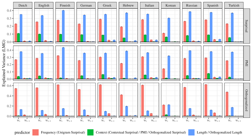
Figure 1: Proportion of total variance explained by the predictors (Kruskal, 1987), across languages and linear regression models. Summing the values represented by the four bars yields the coefficient of determination $R^{2}$. Note that the $R^{2}$ values are the same across the three models, as a consequence of the collinearity discussed in § 2.4. Error bars are 95% confidence intervals across folds of data. We observe only a small proportion of explained variance by context when excluding the variance it shares with frequency, as in the orthogonalized surprisal predictor.

We now seek an empirical understanding of how the new orthogonalized surprisal predictor influences the importance attributed to context in reading time prediction. In addition to the experiment presented here, we also compared the predictive power for nonlinear models across different predictors. Those experiments are discussed in App. F.

Dataset and Predictors.

We use gaze duration times from the Multilingual Eye-movement Corpus (MECO; Siegelman et al., 2022), which consists of word-level eye-tracking measurements from several languages. To obtain surprisal estimates, we approximate ${{p_{\mathrm{H}}}}$ with mGPT (Shliazhko et al., 2024), which is a multilingual LM based on the GPT-2 architecture. The frequency estimates are from Speer (2022) and PMI is computed through the decomposition given in Eq. 10b. Orthogonalized surprisal is obtained by approximating $\langle{\mathbf{I}_{\mathrm{H}}},{\mathbf{Y}_{\mathrm{H}}}\rangle$ and $\langle{\mathbf{Y}_{\mathrm{H}}},{\mathbf{Y}_{\mathrm{H}}}\rangle$ on a training corpus. More specifically, we transform surprisal and frequency to be mean-centered, and use the transformed data to compute unbiased sample variances and covariances. Those sample estimates are then plugged into Eq. 14. § B.2 gives the formula for a linear model with orthogonalized surprisal. We also include a word length predictor. Word length is correlated with frequency (Zipf, 1949), so we orthogonalize it in the same manner as surprisal. App. E gives more details on the dataset and predictor variables.

Experimental Setup.

We fit three linear models using ordinary least squares, with predictors: (i) surprisal, frequency, and length, (ii) PMI, frequency, and length, and (iii) orthogonalized surprisal, frequency, and orthogonalized length. author=Ethan,color=orange!40,size=,fancyline,caption=,]Add: "Orthogonalized surprisal and orthogonalized PMI yeild the same predictor, which we note simply as orthogonalized in figures" (mention brief explaination of why?)  andreas: This is mentioned in fn 8, but I see how that can be easily missed… We include spillover effects from the previous word and fit models over ten folds of cross-validation. We then measure the relative importance of predictors by averaging over the proportion of variance explained by the predictors across orderings in which they are added to the model (Lindeman et al., 1980; Kruskal, 1987), a technique known as LMG (Grömping, 2007). One advantage of this technique, compared to previous methods (e.g., Delta Log Likelihood; Goodkind and Bicknell, 2018) is that LMG gives a better absolute sense of predictive power.

Results.

The LMG values for the different predictors across these models are visualized in Fig. 1. Comparing the plots on the bottom row to the plots on the top row, we observe that the explained variance for orthogonalized surprisal is much lower than for surprisal. These results are consistent across languages. For most languages, when ranking the importance of the predictors, orthogonalization shifts the third most important predictor from context to the previous word’s frequency. Our results suggest that using surprisal therefore overestimates the importance that context has on reading time. Finally, we observe values for PMI that for most languages lie between those for surprisal and orthogonalized surprisal, indicating that the extent to which that PMI overestimates the context effect is smaller compared to surprisal. We observe that the mean $R^{2}$ values of the models across LMG orderings, i.e., the sums of the bars within each facet, range between $0.6$–$0.8$, indicating that the linear models capture a fairly large proportion of the variance observed during the reading process.

5 Conclusion

This article discusses predictors that capture how the processing effort of a unit is shaped by its context. We made the observation that there exist alternatives to the widely used surprisal predictor. Surprisal is correlated with non-contextual frequency, so we provided a technique to disentangle contextual and non-contextual information in language models. In so doing, we found that the effect that context has on reading times appears to be small.

Limitations

Our approach takes one predictor to remain untouched (i.e., frequency), and modifies others to reflect effects that are disassociated from the first. It would thus be natural to ask what happens in the alternative setting, where surprisal remains untouched and frequency is projected onto the orthogonal complement of surprisal. In § F.1, we provide such an analysis. It turns out that even when attributing the shared effect of frequency and surprisal on reading times to surprisal—which is the case when replacing frequency by an orthogonalized frequency predictor—the variance explained by the frequency predictor is still higher for most languages in comparison to the surprisal predictor. This gives further support to our conclusion that context appears to play a small role in reading time prediction.

Furthermore, our presentation of ideas and discussion largely ignores effects of word lengths. We find word lengths to explain the most variance in reading times in our surprisal and PMI models. In addition, after residualizing word length against frequency, we find length to be the second strongest predictor, with an explained variance ranging from around $10\%$–$21\%$. One hypothesis is that readers may make multiple saccades within first passes of longer words, and the time it takes to plan and execute these saccades could be the underlying reason why orthogonalized word length remains explanatory even after residualization. Future work could control for this by adding in the number of saccades within a word as an additional predictor into models.

We are unaware of any efficient algorithm to compute $\langle{\mathbf{I}_{\mathrm{H}}},{\mathbf{Y}_{\mathrm{H}}}\rangle$ and $\langle{\mathbf{Y}_{\mathrm{H}}},{\mathbf{Y}_{\mathrm{H}}}\rangle$ exactly, so in practical settings we must rely on estimation. Thus, it may be that the orthogonalized surprisal predictor is only “close to” being orthogonal to frequency in practice. The manner in which estimation is performed makes our technique similar to residualization—see App. D for a discussion. Moreover, our method only provides guarantees for predictor variables that live in ${\mathcal{H}}$.

Another limitation of this work is that, while we investigate several languages, these are still biased towards Indo-European languages. For example, we present results from one language only for Fino-Uralic, Semitic, Turkic, and Koreanic language families, but seven Indo-European languages. Expanding these results to even more languages would further broaden the impact of this work. In addition, we observe somewhat unique effects for Korean, where, in orthogonalized models, frequency accounts for a lower proportion of the variance, and length and context account for higher proportions, at least compared to other languages. One possible reason for this is the Korean script (Hangul), which combines features of both alphabetic and syllabic writing systems. Future work should conduct similar analyses on different Korean datasets to determine whether this trend is a property of Korean, or just our particular Korean language dataset.

Ethical Considerations

This work uses previously collected human data from the MECO dataset. Please see the paper that introduces this dataset (Siegelman et al., 2022) for information about the data collection procedure. The authors foresee no ethical problems arising from the work presented here.

Appendix A Normalizing the Prefix Probabilities

Here we show that ${{Z}_{\pi_{\mathrm{H}}}}$ as defined in Eq. 2 is the normalizing constant for the prefix probabilities.

Proposition 1.

Let ${{Z}_{\pi_{\mathrm{H}}}}$ be defined as in Eq. 2, i.e.,

$${{Z}_{\pi_{\mathrm{H}}}}=1+\sum_{{\boldsymbol{u}}\in{\Sigma}^{*}}{{p_{\mathrm{H}}}}({\boldsymbol{u}})|{\boldsymbol{u}}|.$$ (16)

Then, ${{Z}_{\pi_{\mathrm{H}}}}$ is the normalizing constant for ${\pi_{\mathrm{H}}}$, i.e.,

$$\sum_{{\boldsymbol{c}}\in{\Sigma}^{*}}{\pi_{\mathrm{H}}}({\boldsymbol{c}})=1.$$ (17)

Proof.

First, note that Eq. 2 can be rewritten in the following manner:

$${{Z}_{\pi_{\mathrm{H}}}} =1+\sum_{{\boldsymbol{u}}\in{\Sigma}^{*}}{{p_{\mathrm{H}}}}({\boldsymbol{u}})|{\boldsymbol{u}}|$$ (18a)

$$=\sum_{{\boldsymbol{u}}\in{\Sigma}^{*}}{{p_{\mathrm{H}}}}({\boldsymbol{u}})+\sum_{{\boldsymbol{u}}\in{\Sigma}^{*}}{{p_{\mathrm{H}}}}({\boldsymbol{u}})|{\boldsymbol{u}}|$$ (18b)

$$=\sum_{{\boldsymbol{u}}\in{\Sigma}^{*}}(1+|{\boldsymbol{u}}|){{p_{\mathrm{H}}}}({\boldsymbol{u}})$$ (18c)

$$=\sum_{{\boldsymbol{c}}\in{\Sigma}^{*}}\sum_{{\boldsymbol{u}}^{\prime}\in{\Sigma}^{*}}{{p_{\mathrm{H}}}}({\boldsymbol{c}}{\boldsymbol{u}}^{\prime}).$$ (18d)

The last step follows from the fact that a string ${\boldsymbol{u}}$ can be segmented into two substrings ${\boldsymbol{c}}$ and ${\boldsymbol{u}}^{\prime}$ in $1+|{\boldsymbol{u}}|$ ways. Note the two cases where either ${\boldsymbol{c}}={\varepsilon}$ and ${\boldsymbol{u}}^{\prime}={\boldsymbol{u}}$, or ${\boldsymbol{c}}={\boldsymbol{u}}$ and ${\boldsymbol{u}}^{\prime}={\varepsilon}$ (with ${\varepsilon}$ denoting the empty string). It is then easy to see that ${{Z}_{\pi_{\mathrm{H}}}}$ is a valid normalizing constant:

$$\sum_{{\boldsymbol{c}}^{\prime}\in{\Sigma}^{*}}{\pi_{\mathrm{H}}}({\boldsymbol{c}}^{\prime}) =\sum_{{\boldsymbol{c}}^{\prime}\in{\Sigma}^{*}}\frac{\sum_{{\boldsymbol{u}}\in{\Sigma}^{*}}{{p_{\mathrm{H}}}}({\boldsymbol{c}}^{\prime}{\boldsymbol{u}})}{\sum_{{\boldsymbol{c}}\in{\Sigma}^{*}}\sum_{{\boldsymbol{u}}^{\prime}\in{\Sigma}^{*}}{{p_{\mathrm{H}}}}({\boldsymbol{c}}{\boldsymbol{u}}^{\prime})}$$ (19a)

$$=\frac{\sum_{{\boldsymbol{c}}^{\prime}\in{\Sigma}^{*}}\sum_{{\boldsymbol{u}}\in{\Sigma}^{*}}{{p_{\mathrm{H}}}}({\boldsymbol{c}}^{\prime}{\boldsymbol{u}})}{\sum_{{\boldsymbol{c}}\in{\Sigma}^{*}}\sum_{{\boldsymbol{u}}^{\prime}\in{\Sigma}^{*}}{{p_{\mathrm{H}}}}({\boldsymbol{c}}{\boldsymbol{u}}^{\prime})}$$ (19b)

$$=1.$$ (19c)

∎

Appendix B Linear Models

B.1 Rewriting Linear Models with Surprisal in Terms of PMI

In this section, we demonstrate the equivalence between two linear models, one with surprisal and frequency as predictors, and the other with PMI and frequency as predictors. In particular, we consider a linear model of reading times ${f_{{\boldsymbol{\beta}}}}\left(\;\cdot\mid{\mathbf{X}}({\boldsymbol{c}},{\overline{{u}}})\right)$, in which ${\mathbf{X}}({\boldsymbol{c}},{\overline{{u}}})\colon{\Sigma}^{*}\times{\overline{{\Sigma}}}\rightarrow{\mathbb{R}^{D}}$ includes surprisal, frequency and additional baseline predictors ${{\mathbf{X}}_{\text{b}}}({\boldsymbol{c}},{\overline{{u}}})\colon{\Sigma}^{*}\times{\overline{{\Sigma}}}\rightarrow\mathbb{R}^{D-3}$ and show that it is equivalent to a model in which surprisal is replaced with PMI. Consider the prediction ${\widehat{{r}}}({\boldsymbol{c}},{\overline{{u}}})$ which is the expected value of ${f_{{\boldsymbol{\beta}}}}\left(\;\cdot\mid{\mathbf{X}}({\boldsymbol{c}},{\overline{{u}}})\right)$. To demonstrate the equivalence, we simply add and subtract an additional frequency term:

$${\widehat{{r}}}({\boldsymbol{c}},{\overline{{u}}}) ={\beta_{0}}+{\beta_{{\upsilon_{\mathrm{H}}}}}{\upsilon_{\mathrm{H}}}({\overline{{u}}})+{\beta_{{\iota_{\mathrm{H}}}}}{\iota_{\mathrm{H}}}({\boldsymbol{c}},{\overline{{u}}})+{\boldsymbol{\beta}^{\intercal}_{\text{b}}}{{\mathbf{X}}_{\text{b}}}({\boldsymbol{c}},{\overline{{u}}})$$ (20a)

$$={\beta_{0}}+({\beta_{{\upsilon_{\mathrm{H}}}}}+{\beta_{{\iota_{\mathrm{H}}}}}){\upsilon_{\mathrm{H}}}({\overline{{u}}})-{\beta_{{\iota_{\mathrm{H}}}}}(\underbrace{{\upsilon_{\mathrm{H}}}({\overline{{u}}})-{\iota_{\mathrm{H}}}({\boldsymbol{c}},{\overline{{u}}})}_{={\mu_{\mathrm{H}}}({\boldsymbol{c}},{\overline{{u}}})})+{\boldsymbol{\beta}^{\intercal}_{\text{b}}}{{\mathbf{X}}_{\text{b}}}({\boldsymbol{c}},{\overline{{u}}})$$ (20b)

$$={\beta_{0}}+({\beta_{{\upsilon_{\mathrm{H}}}}}+{\beta_{{\iota_{\mathrm{H}}}}}){\upsilon_{\mathrm{H}}}({\overline{{u}}})-{\beta_{{\iota_{\mathrm{H}}}}}{\mu_{\mathrm{H}}}({\boldsymbol{c}},{\overline{{u}}})+{\boldsymbol{\beta}^{\intercal}_{\text{b}}}{{\mathbf{X}}_{\text{b}}}({\boldsymbol{c}},{\overline{{u}}}),$$ (20c)

where ${\boldsymbol{\beta}}=[{\beta_{0}},{\beta_{{\upsilon_{\mathrm{H}}}}},{\beta_{{\iota_{\mathrm{H}}}}},{\boldsymbol{\beta}}_{\text{b}}]\in{\mathbb{R}^{D}}$.

B.2 The Orthogonalized Surprisal Model

Under a linear model of reading time which includes orthogonal surprisal, frequency and (possibly) other predictors ${{\mathbf{X}}_{\text{b}}}({\boldsymbol{c}},{\overline{{u}}})$, reading time predictions are obtained as follows:

$${\widehat{{r}}}({\boldsymbol{c}},{\overline{{u}}}) ={\beta_{0}}+{\beta_{{\iota_{\mathrm{H}}}}}\left({\iota_{\mathrm{H}}}({\boldsymbol{c}},{\overline{{u}}})-\frac{{\mathrm{Cov}}({\mathbf{I}_{\mathrm{H}}},{\mathbf{Y}_{\mathrm{H}}})}{{\mathrm{Cov}}({\mathbf{Y}_{\mathrm{H}}},{\mathbf{Y}_{\mathrm{H}}})}{\upsilon_{\mathrm{H}}}({\overline{{u}}})\right)+{\beta_{{\upsilon_{\mathrm{H}}}}}{\upsilon_{\mathrm{H}}}({\overline{{u}}})+{\boldsymbol{\beta}^{\intercal}_{\text{b}}}{{\mathbf{X}}_{\text{b}}}({\boldsymbol{c}},{\overline{{u}}})$$ (21a)

$$={\beta_{0}}+{\beta_{{\iota_{\mathrm{H}}}}}{\iota_{\mathrm{H}}}({\boldsymbol{c}},{\overline{{u}}})+\left({\beta_{{\upsilon_{\mathrm{H}}}}}-{\beta_{{\iota_{\mathrm{H}}}}}\frac{{\mathrm{Cov}}({\mathbf{I}_{\mathrm{H}}},{\mathbf{Y}_{\mathrm{H}}})}{{\mathrm{Cov}}({\mathbf{Y}_{\mathrm{H}}},{\mathbf{Y}_{\mathrm{H}}})}\right){\upsilon_{\mathrm{H}}}({\overline{{u}}})+{\boldsymbol{\beta}^{\intercal}_{\text{b}}}{{\mathbf{X}}_{\text{b}}}({\boldsymbol{c}},{\overline{{u}}}).$$ (21b)

We estimate ${\mathrm{Cov}}({\mathbf{I}_{\mathrm{H}}},{\mathbf{Y}_{\mathrm{H}}})$ (and ${\mathrm{Cov}}({\mathbf{Y}_{\mathrm{H}}},{\mathbf{Y}_{\mathrm{H}}})$) through the unbiased sample covariance on the training corpus,

$$\frac{1}{N-1}\sum_{{\overline{{u}}}\in{\overline{{\Sigma}}}}({\iota_{\mathrm{H}}}({\boldsymbol{c}},{\overline{{u}}})-{\hat{\mu}}_{\iota_{\mathrm{H}}})({\upsilon_{\mathrm{H}}}({\overline{{u}}})-{\hat{\mu}}_{\upsilon_{\mathrm{H}}}),$$ (22)

where ${\hat{\mu}}_{\iota_{\mathrm{H}}}$ and ${\hat{\mu}}_{\upsilon_{\mathrm{H}}}$ are the training corpus sample means for surprisal and frequency, respectivey.

Appendix C Further Technical Details on the Hilbert Space

In this section we provide formal guarantees for the method presented in § 3. In § C.1, we justify why the Hilbert space introduced in § 3 is indeed a Hilbert space. In § C.2, we show that the projection in Eq. 14 yields a predictor which is orthogonal to frequency.

C.1 Predictor Variables as Elements of a Hilbert Space

Let $({\Sigma}^{*}\times{\overline{{\Sigma}}},\mathcal{P}({\Sigma}^{*}\times{\overline{{\Sigma}}}),{{\pi_{\mathrm{H}}}\cdot{{p_{\mathrm{H}}}}})$ be a probability space. We further require that ${\pi_{\mathrm{H}}}({\boldsymbol{c}}){{p_{\mathrm{H}}}}({\overline{{u}}}\mid{\boldsymbol{c}})>0$ for all ${\boldsymbol{c}}\in{\Sigma}^{*}$ and ${u}\in{\Sigma}$, which is equivalent to the assumption that ${{p_{\mathrm{H}}}}({\boldsymbol{u}})>0$ for all ${\boldsymbol{u}}\in{\Sigma}^{*}$ by Eqs. 3 and 4. We construct a Hilbert space ${\mathcal{H}}$ over ${\mathbb{R}}$ of all random variables of type ${\mathbf{X}}\colon{\Sigma}^{*}\times{\overline{{\Sigma}}}\rightarrow{\mathbb{R}}$ with the restriction that $\mathbb{E}[{\mathbf{X}}^{2}]<\infty$. We require the second moment to be finite since $\infty\notin{\mathbb{R}}$. In this paper, we are particularly interested in the random variables ${\mathbf{I}_{\mathrm{H}}}({\boldsymbol{c}},{\overline{{u}}})={\iota_{\mathrm{H}}}({\boldsymbol{c}},{\overline{{u}}})$, ${\mathbf{M}_{\mathrm{H}}}({\boldsymbol{c}},{\overline{{u}}})={\mu_{\mathrm{H}}}({\boldsymbol{c}},{\overline{{u}}})$, ${\mathbf{Y}_{\mathrm{H}}}({\boldsymbol{c}},{\overline{{u}}})={\upsilon_{\mathrm{H}}}({\overline{{u}}})$, for ${\boldsymbol{c}}\in{\Sigma}^{*}$ and ${\overline{{u}}}\in{\overline{{\Sigma}}}$. They encode the distributions over surprisal, frequency and PMI, respectively, and are all distributed according to ${{\pi_{\mathrm{H}}}\cdot{{p_{\mathrm{H}}}}}$. We have

$$\mathbb{P}({\mathbf{I}_{\mathrm{H}}}=\iota)=\sum_{\begin{subarray}{c}{\boldsymbol{c}}\in{\Sigma}^{*},\\ {\overline{{u}}}\in{\overline{{\Sigma}}}\end{subarray}}{\pi_{\mathrm{H}}}({\boldsymbol{c}}){{p_{\mathrm{H}}}}({\overline{{u}}}\mid{\boldsymbol{c}})\mathbbm{1}\{\iota={\iota_{\mathrm{H}}}({\boldsymbol{c}},{\overline{{u}}})\}$$ (23a)

$$\mathbb{P}({\mathbf{Y}_{\mathrm{H}}}=\upsilon)=\sum_{\begin{subarray}{c}{\boldsymbol{c}}\in{\Sigma}^{*},\\ {\overline{{u}}}\in{\overline{{\Sigma}}}\end{subarray}}{\pi_{\mathrm{H}}}({\boldsymbol{c}}){{p_{\mathrm{H}}}}({\overline{{u}}}\mid{\boldsymbol{c}})\mathbbm{1}\{\upsilon={\upsilon_{\mathrm{H}}}({\overline{{u}}})\}$$ (23b)

$$\mathbb{P}({\mathbf{M}_{\mathrm{H}}}=\mu)=\sum_{\begin{subarray}{c}{\boldsymbol{c}}\in{\Sigma}^{*},\\ {\overline{{u}}}\in{\overline{{\Sigma}}}\end{subarray}}{\pi_{\mathrm{H}}}({\boldsymbol{c}}){{p_{\mathrm{H}}}}({\overline{{u}}}\mid{\boldsymbol{c}})\mathbbm{1}\{\mu={\mu_{\mathrm{H}}}({\boldsymbol{c}},{\overline{{u}}})\}.$$ (23c)

We define the following inner product:

$$\langle{\mathbf{X}},{\mathbf{Y}}\rangle \mathrel{\stackrel{{\scriptstyle\textnormal{def}}}{{=}}}\mathbb{E}\left[{\mathbf{X}}{\mathbf{Y}}\right]$$ (24a)

$$=\sum_{\begin{subarray}{c}{\boldsymbol{c}}\in{\Sigma}^{*},\\ {\overline{{u}}}\in{\overline{{\Sigma}}}\end{subarray}}{\pi_{\mathrm{H}}}({\boldsymbol{c}}){{p_{\mathrm{H}}}}({\overline{{u}}}\mid{\boldsymbol{c}}){\mathbf{X}}({\boldsymbol{c}},{\overline{{u}}}){\mathbf{Y}}({\boldsymbol{c}},{\overline{{u}}}).$$ (24b)

Consequently, the norm is given by ${||\cdot||_{{\mathcal{H}}}}\mathrel{\stackrel{{\scriptstyle\textnormal{def}}}{{=}}}\sqrt{\langle\cdot,\cdot\rangle}$ and the distance metric between two random variables ${\mathbf{X}}$ and ${\mathbf{Y}}$ is ${d}({\mathbf{X}},{\mathbf{Y}})\mathrel{\stackrel{{\scriptstyle\textnormal{def}}}{{=}}}{||{\mathbf{X}}-{\mathbf{Y}}||_{{\mathcal{H}}}}$. With this choice of inner product, ${\mathcal{H}}$ is a Hilbert space. That is because ${\mathcal{H}}$ is the $L^{2}({\Sigma}^{*}\times{\overline{{\Sigma}}})$ space, and any such $L^{2}$ space is a Hilbert space (Rudin, 1987, p. 78).

C.2 Orthogonal Projection

In this section, we use the Hilbert projection theorem to show that frequency and orthogonalized surprisal are disentangled, i.e., that $\langle{\mathbf{Y}_{\mathrm{H}}},\mathrm{proj}_{{\mathbf{Y}^{\perp}_{\mathrm{H}}}}({\mathbf{I}_{\mathrm{H}}})\rangle=0$. We introduce the Hilbert projection theorem in Prop. 2 and apply it to our technique in Prop. 3.

Proposition 2 (Hilbert Projection Theorem).

Let ${\mathcal{H}}$ be a Hilbert space and ${\mathcal{C}}\subseteq{\mathcal{H}}$ be a nonempty closed convex set. For every ${\mathbf{X}}\in{\mathcal{H}}$ there exists a unique ${||{\mathbf{X}}-{\mathbf{Y}}^{\prime}||_{{\mathcal{H}}}}$ which is equal to

$$\inf_{{\mathbf{Y}}\in{\mathcal{C}}}{||{\mathbf{X}}-{\mathbf{Y}}||_{{\mathcal{H}}}}.$$ (25)

If ${\mathcal{C}}$ is a closed vector subspace of ${\mathcal{H}}$, then ${\mathbf{X}}-{\mathbf{Y}}^{\prime}$ is orthogonal to ${\mathcal{C}}$, i.e., $\langle{\mathbf{X}}-{\mathbf{Y}}^{\prime},{\mathbf{Y}}\rangle=0$ for all ${\mathbf{Y}}\in{\mathcal{C}}$.

Proof.

See Rudin (1991, pp. 306-9). ∎

Proposition 3 (Decorrelated Predictors).

Let ${\mathcal{H}}$ be the Hilbert space introduced in § 3 and § C.1. Further, consider ${\mathbf{X}},{\mathbf{Z}}\in{\mathcal{H}}$ and define

$$\mathrm{proj}_{{\mathbf{Z}}^{\perp}}({\mathbf{X}})\mathrel{\stackrel{{\scriptstyle\textnormal{def}}}{{=}}}{\mathbf{X}}-\frac{\langle{\mathbf{X}},{\mathbf{Z}}\rangle}{\langle{\mathbf{Z}},{\mathbf{Z}}\rangle}{\mathbf{Z}}.$$ (26)

Then,

$$\langle\mathrm{proj}_{{\mathbf{Z}}^{\perp}}({\mathbf{X}}),{\mathbf{Z}}\rangle=0.$$ (27)

Proof.

Let ${\mathcal{C}}$ be the set of vectors spanned by ${\mathbf{Z}}$, i.e., ${\mathcal{C}}\mathrel{\stackrel{{\scriptstyle\textnormal{def}}}{{=}}}\{a{\mathbf{Z}}\mid a\in{\mathbb{R}}\}$. It is easy to see that ${\mathcal{C}}$ is a closed subspace of ${\mathcal{H}}$. Then, by Prop. 2, there exists a ${\mathbf{Y}}^{\prime}$ such that

$$\inf_{{\mathbf{Y}}\in{\mathcal{C}}}{||{\mathbf{X}}-{\mathbf{Y}}||_{{\mathcal{H}}}}={||{\mathbf{X}}-{\mathbf{Y}}^{\prime}||_{{\mathcal{H}}}}.$$ (28)

By the definition of ${\mathcal{C}}$, we have ${\mathbf{Y}}^{\prime}=a^{\prime}{\mathbf{Z}}$ for some $a^{\prime}\in{\mathbb{R}}$. Because the infimum is achieved, to determine $a^{\prime}$, we consider the following convex optimization problem:

$$\operatorname*{{\mathrm{argmin}}}_{a\in{\mathbb{R}}}{||{\mathbf{X}}-a{\mathbf{Z}}||^{2}_{{\mathcal{H}}}} =\operatorname*{{\mathrm{argmin}}}_{a\in{\mathbb{R}}}{||a{\mathbf{Z}}||^{2}_{{\mathcal{H}}}}-2\langle a{\mathbf{Z}},{\mathbf{X}}\rangle+{||{\mathbf{X}}||^{2}_{{\mathcal{H}}}}$$ (29a)

$$=\operatorname*{{\mathrm{argmin}}}_{a\in{\mathbb{R}}}a^{2}{||{\mathbf{Z}}||^{2}_{{\mathcal{H}}}}-2a\langle{\mathbf{Z}},{\mathbf{X}}\rangle.$$ (29b)

Because Eq. 29b is differentiable in $a$, we check the first-order optimality conditions

$$2a{||{\mathbf{Z}}||^{2}_{{\mathcal{H}}}}-2\langle{\mathbf{Z}},{\mathbf{X}}\rangle=0,$$ (30)

so

$$\operatorname*{{\mathrm{argmin}}}_{a\in{\mathbb{R}}}a^{2}{||{\mathbf{Z}}||^{2}_{{\mathcal{H}}}}-2a\langle{\mathbf{Z}},{\mathbf{X}}\rangle =\frac{\langle{\mathbf{Z}},{\mathbf{X}}\rangle}{{||{\mathbf{Z}}||^{2}_{{\mathcal{H}}}}}$$ (31a)

$$=\frac{\langle{\mathbf{Z}},{\mathbf{X}}\rangle}{\langle{\mathbf{Z}},{\mathbf{Z}}\rangle}.$$ (31b)

We note that this solution is unique because Eq. 29b is convex in $a$. Thus, observing by Prop. 2 that

$$\langle{\mathbf{X}}-\frac{\langle{\mathbf{Z}},{\mathbf{X}}\rangle}{\langle{\mathbf{Z}},{\mathbf{Z}}\rangle}{\mathbf{Z}},{\mathbf{Z}}\rangle=0,$$ (32)

we have the desired result that $\langle\mathrm{proj}_{{\mathbf{Z}}^{\perp}}({\mathbf{X}}),{\mathbf{Z}}\rangle=0$. ∎

Appendix D Our Method in Relation to Residualization

The technique presented in § 3 closely resembles another method used to decorrelate predictors—residualization (see, e.g., Kuperman et al., 2008; Jaeger, 2010; García et al., 2019). Consider a linear regression setting with response ${\mathbf{y}}\in{{\mathbb{R}}^{N}}$ and design matrix ${\mathbf{X}}\in{{\mathbb{R}}^{{N}\times 2}}$, i.e., ${N}$ data points for two predictors ${\mathbf{x}_{1}},{\mathbf{x}_{2}}\in{{\mathbb{R}}^{N}}$, being column vectors. The idea behind residualization is to decorrelate the predictors by replacing one of them, say ${\mathbf{x}_{1}}$, by the residuals obtained from the ordinary least squares solution of the regression model in which ${\mathbf{x}_{1}}$ is the response and ${\mathbf{x}_{2}}$ is the (only) predictor. The new predictor will thus take the value

$${\mathbf{x}_{1\text{-res}}}={\mathbf{x}_{1}}-({\hat{\beta}^{\text{ols}}_{0}}+{\hat{\beta}^{\text{ols}}_{1}}{\mathbf{x}_{2}}),$$ (33)

where ${\hat{\beta}^{\text{ols}}_{0}},{\hat{\beta}^{\text{ols}}_{1}}\in{\mathbb{R}}$ are the ordinary least squares estimates for the intercept and slope, respectively, when regressing ${\mathbf{x}_{1}}$ against ${\mathbf{x}_{2}}$. Note that ${\hat{\beta}^{\text{ols}}_{0}}=0$ and ${\hat{\beta}^{\text{ols}}_{1}}=\frac{{\mathbf{x}_{1}}^{\intercal}{\mathbf{x}_{2}}}{{\mathbf{x}_{2}}^{\intercal}{\mathbf{x}_{2}}}$ under mean centering. In that case, Eq. 33 mirrors Eq. 14:

$${\mathbf{x}_{1\text{-res}}}={\mathbf{x}_{1}}-\frac{{\mathbf{x}_{1}}^{\intercal}{\mathbf{x}_{2}}}{{\mathbf{x}_{2}}^{\intercal}{\mathbf{x}_{2}}}{\mathbf{x}_{2}},$$ (34)

In Eq. 14 we had the inner product between two vectors in the Hilbert space ${\mathcal{H}}$, but here we have the inner product between two vectors in Euclidean space (${\mathbf{x}_{1}}$ and ${\mathbf{x}_{2}}$), which is the dot product. Indeed, residualization is defined only over a sample of data points. Our technique can thus be viewed as a functional generalization of residualization. From a statistical perspective, Eq. 34 provides estimates of residual values which can, ideally, be generalized to data beyond the sample of ${N}$ data points from which they were estimated. In a Hilbert space, on the other hand, there is no question of generalization. For the predictors we use, which are derived from a language model, we know their true values. We only approximate the inner products in Eq. 14 since computing their exact value would be intractable. That is, the reason for our approximation, which yields the same formula as residualization, is computational, rather than statistical.

Arguments Against Residualization.

Residualization has received criticism as a way to obtain more interpretable model coefficients (York, 2012; Wurm and Fisicaro, 2014). Consider the following three linear regression models estimated by ordinary least squares:

$$\text{Model A}\colon\quad {\mathbf{y}}=\beta^{A}_{0}+\beta^{A}_{1}{\mathbf{x}_{1}}+\beta^{A}_{2}{\mathbf{x}_{2}}+\boldsymbol{\varepsilon}$$ (35)

$$\text{Model B}\colon\quad {\mathbf{y}}=\beta^{B}_{0}+\beta^{B}_{1}{\mathbf{x}_{1\text{-res}}}+\beta^{B}_{2}{\mathbf{x}_{2}}+\boldsymbol{\varepsilon}$$ (36)

$$\text{Model C}\colon\quad {\mathbf{y}}=\beta^{C}_{0}+\beta^{C}_{2}{\mathbf{x}_{2}}+\boldsymbol{\varepsilon},$$ (37)

where $\boldsymbol{\varepsilon}\in{{\mathbb{R}}^{N}}$ is a vector of Gaussian noise variables. In the models above, we have that $\beta^{A}_{1}=\beta^{B}_{1}$ and $\beta^{A}_{2}\neq\beta^{B}_{2}=\beta^{C}_{2}$ (Wurm and Fisicaro, 2014). That is, the effect of the residualized predictor—${\mathbf{x}_{1}}$ in the example above—remains the same after residualization (Model A vs. Model B). On the other hand, the estimated effect of the residualizing predictor on the response—${\mathbf{x}_{2}}$ in the example above—changes between Model B which regresses ${\mathbf{y}}$ on ${\mathbf{x}_{1\text{-res}}}$ and ${\mathbf{x}_{2}}$ and Model A which regresses ${\mathbf{y}}$ on ${\mathbf{x}_{1}}$ and ${\mathbf{x}_{2}}$. The estimated effect of ${\mathbf{x}_{2}}$ in Model B instead becomes equal to what it would have been under a model with a single predictor, regressing only on ${\mathbf{x}_{2}}$ (Model C). These outcomes are contrary to what one might expect: The effect of the modified, residualized predictor ${\mathbf{x}_{1}}$ is the same while the effect of the untouched predictor ${\mathbf{x}_{2}}$ changes. This has indeed been a source of confusion in the literature (Wurm and Fisicaro, 2014). However, in our case, the fact that $\beta^{A}_{2}\neq\beta^{B}_{2}=\beta^{C}_{2}$ is actually the desired consequence: We sought to estimate the effect of context that is not correlated with frequency. In other words, we want the covariance between frequency and surprisal to be attributed to frequency, as it would be in a model that only regresses reading time on frequency (corresponding to Model C). Moreover, we argue that the estimated coefficient is the wrong quantity to look at when measuring importance—it is the role of the predictor in relation to the others that should matter. While $\beta^{A}_{1}=\beta^{B}_{1}$ does not indicate a difference in importance, a measure of explained variance like LMG does, as we demonstrate by our results in Fig. 1. We thus advocate for the use of such a measure instead of analyzing coefficients. Another remark relates to whether a residualized variable is interpretable as anything at all. For instance, Breaugh (2006) gives an example of height and weight of basketball players: Residualizing height with respect to weight would result in a residualized predictor that would involve a notion of height disentangled from weight, which is tricky to conceptualize in a real-world context. However, in our case, we are addressing the question of what predictor should be extracted in the first place, i.e., from a language model as a stand-in for context. Our paper argued that orthogonalized surprisal gives a better interpretation for the effect of context than contextual surprisal does.

We hope that our work and this discussion can help shed further light on when residualization is, and is not, suitable.

Appendix E Dataset and Predictor Variables

E.1 Dataset

We use the Multilingual Eye-movement Corpus (MECO; Siegelman et al., 2022), which consists of eye-tracking-based reading-time data across 13 different languages for 12 Wikipedia-style articles about various topics. The articles have been carefully constructed to contain the same content across languages. Word-level reading time is recorded for between $32{-}54$ participants per language, using several different reading variables. Of these, for our main experiments, we use gaze duration, which is the total fixation time on a word during its first pass (i.e., before the first time the gaze leaves the word). However, below we also show results for two other reading metrics: first fixation duration, which is the duration of the first fixation that lands on the word, and total fixation duration, which is the sum over all fixation durations of a word. In our experiments, we give a reading time of zero to words that were skipped on the first pass. We take the average over the by-subject reading times to obtain the response variables we model.

E.2 Predictors

Our predictor variables are estimated in the following way: Surprisal estimates are obtained from mGPT (Shliazhko et al., 2024), which is a multilingual variant of GPT-3 that was trained on Wikipedia and the C4 corpus (Raffel et al., 2020). It supports 61 languages, which intersected with the MECO dataset yields 11 languages for our experiments: Dutch, English, Finnish, German, Greek, Hebrew, Italian, Korean, Russian, Spanish, and Turkish. Estonian and Norwegian, which are present in MECO, are unfortunately not supported by mGPT. For each word in MECO, we sum the surprisals estimated by mGPT for each of the tokens that make up that word. We use the estimates from Speer (2022) to obtain word frequency (i.e., unigram surprisal) and length, following previous work. Finally, PMI estimates are obtained from surprisal and frequency through Eq. 10b. All predictors are standardized (i.e., set to mean zero and standard deviation one) before computing orthogonalized surprisal values and fitting the regression models.

Appendix F Additional Experiments

We complement the main experiments presented in § 4 with three additional empirical analyses. In § F.1, we take an alternative position to the one in the main text, using an orthogonalized frequency predictor. In § F.2, we exclude the length predictor and perform the same analysis as we did in the main text. In § F.3, we compare the predictive power of nonlinear models across different sets of predictors.

F.1 Orthogonalized Frequency

Here, we provide an additional analysis in which we derive a new frequency predictor, swapping the two variables in Eq. 14. In this case, the shared effect of frequency and surprisal on reading time is attributed to surprisal, and the frequency effect represents the effect beyond what is already explained by surprisal. We present the results in Fig. 2. Comparing this analysis to Fig. 1 may be considered analogous to Shain’s (2019) study, which compares the independent effects of surprisal and frequency by adding them in as predictors on top of baseline models that contain the other. However, in contrast to Shain (2019), we find that frequency appears to be more important than contextual effects in explaining reading times.

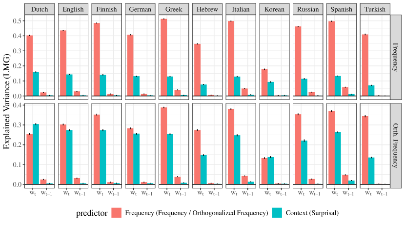
Figure 2: This figure is analogous to Fig. 1, with the difference that frequency is projected onto the orthogonal complement of surprisal, resulting in an orthogonalized frequency predictor. Even when the shared effect of frequency and surprisal is attributed to surprisal, we still find that the frequency predictor explains more variance than surprisal for most languages.

F.2 Results without Length

We complement the experiments in § 4 with an additional analysis which excludes length. We follow the same experimental setup as described in the main portion of the text, this time with three linear models that include predictors: (i) surprisal and frequency, (ii) PMI and frequency, and (iii) orthogonalized surprisal and frequency. We include spillover variables from the previous word. The results are shown in Fig. 3. We observe that the implications on context found in Fig. 1 do not change when excluding length.

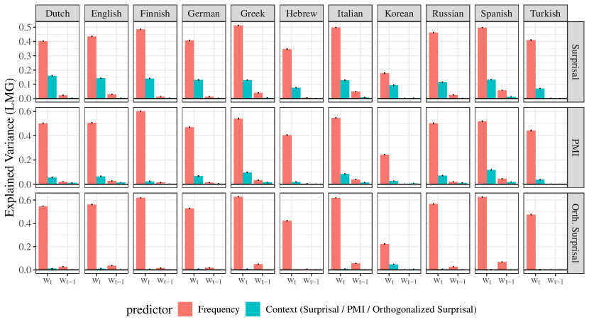
Figure 3: This figure is analogous to Fig. 1, except that it shows results when excluding the word length predictor.

F.3 Psychometric Predictive Power

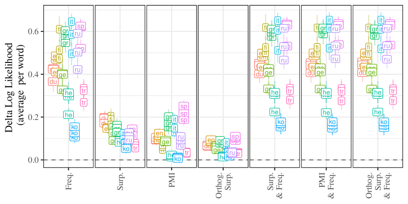
Figure 4: $\Delta_{\mathrm{llh}}$of GAM models. Models include only the indicated predictors. Error bars are 95% confidence intervals across folds of data.

While the surprisal and PMI models are equivalent under a linear model, that relationship does not necessarily need to hold under a nonlinear one. Therefore, we compare the psychometric predictive power by fitting generalized additive models (GAMs). GAMs are a class of additive models that can learn non-linear relationships between predictor and response variables. All the terms in our GAMs are spline-based smooth terms, that include either a contextual predictor variable (i.e., surprisal, PMI, or orthogonalized surprisal), or frequency. We restrict our smooth terms to six basis functions, following the logic outlined in Hoover et al. (2023). GAMs are fit using the mgcv package in R. Two example calls are given below:

⬇

gam(reading_time ~ s(surprisal, bs = ’cr’, k = 6) + s(prev_surprisal, bs = ’cr’, k = 6), data = .)

gam(reading_time ~ s(pmi, bs = ’cr’, k = 6) + s(prev_pmi, bs = ’cr’, k = 6) + s(frequency, bs = ’cr’, k = 6) + s(prev_frequency, bs = ’cr’, k = 6), data = .)

We consider an additional baseline model which is the average reading time estimated from the training set. We compare delta log-likelihood $\Delta_{\mathrm{llh}}$—the average difference in likelihood between the target models mentioned above and the baseline model—as estimated over ten folds of cross-validation across several different sets of predictor variables.

Results are visualized in Fig. 4. We observe three big trends: First, we find that all predictors lead to positive $\Delta_{\mathrm{llh}}$, indicating that they are useful for predicting reading times. However, second, when looking at models with just one predictor variable, we observe that frequency alone leads to higher $\Delta_{\mathrm{llh}}$than any other single variable, and that surprisal and PMI tend to result in higher $\Delta_{\mathrm{llh}}$than orthogonalized surprisal. This is to be expected. We know from prior research that frequency plays a large role in explaining by-word processing effort, and because orthogonalized variables, by definition, are decorrelated with frequency, they are not expected to be strong predictors of reading times, alone.

The right three facets of Fig. 4 show models that combine contextual and non-contextual predictors into a single model. Here, we observe only insignificant, nearly invisible differences between the models’ ${\Delta_{\mathrm{llh}}}$. We conclude that all three implementations of context are equally good at predicting reading times.

In Fig. 5, we show our generalized additive modeling results, broken down by language, across the $x$-facets. We also show results for reading time metrics other than gaze duration, including first fixation duration (top row) and total reading times (bottom row). These results are consistent with those reported in Fig. 4. We find that of the four individual predictors, frequency leads to the highest $\Delta_{\mathrm{llh}}$, followed by surprisal, PMI, and then orthogonalized variants. When combining our non-contextual predictor (frequency), alongside these contextual predictors, we do not observe differences in $\Delta_{\mathrm{llh}}$.

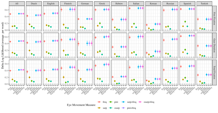
Figure 5: Psychometric Predictive Power by Language. Results are consistent those reported in Fig. 4.

Appendix G Connection with Model Size

The results presented in this article may help explain a trend recently observed in the computational psycholinguistics literature: Surprisal values of larger LMs provide a worse fit to human reading-time data compared to those of medium-sized models (Oh and Schuler, 2023b). Specifically, Oh et al. (2024) suggest that this is because larger models are incredibly accurate at predicting rare words in context. Medium-sized models, on the other hand, are not as good at predicting rare words in context. Therefore, surprisal estimates for these words are closer to their unigram frequencies, i.e., non-contextual surprisal. If reading times are primarily driven by frequency effects, as suggested by our analysis, the surprisal predictor should—on its own—yield stronger predictive power if it is closer to frequency, as is the case for medium-sized models. Thus, this could explain why the decoupling of surprisal and frequency in these larger models results in poorer fits to human reading times.

References

- Boltzmann (1868) Ludwig Boltzmann. 1868. Studien über das Gleichgewicht der lebendigen Kraft zwischen bewegten materiellen Punkten. K.K. Hof und Staatsdruckerei.
- Breaugh (2006) James A. Breaugh. 2006. Rethinking the control of nuisance variables in theory testing. Journal of Business and Psychology, 20(3):429–443.
- Broadbent (1967) Donald E. Broadbent. 1967. Word-frequency effect and response bias. Psychological Review, 74 1:1–15.
- Bybee (2006) Joan Bybee. 2006. Frequency of use and the organization of language. Oxford University Press.
- Church and Hanks (1990) Kenneth Ward Church and Patrick Hanks. 1990. Word association norms, mutual information, and lexicography. Computational Linguistics, 16(1):22–29.
- Demberg and Keller (2008) Vera Demberg and Frank Keller. 2008. Data from eye-tracking corpora as evidence for theories of syntactic processing complexity. Cognition, 109(2):193–210.
- Du et al. (2023) Li Du, Lucas Torroba Hennigen, Tiago Pimentel, Clara Meister, Jason Eisner, and Ryan Cotterell. 2023. A measure-theoretic characterization of tight language models. In Proceedings of the 61st Annual Meeting of the Association for Computational Linguistics (Volume 1: Long Papers), pages 9744–9770, Toronto, Canada. Association for Computational Linguistics.
- Fano (1961) Robert M. Fano. 1961. Transmission of Information: A Statistical Theory of Communication. MIT Press Classics. MIT Press.
- García et al. (2019) Catalina B. García, Román Salmerón, Claudia García, and José García. 2019. Residualization: justification, properties and application. Journal of Applied Statistics, 47(11):1990–2010.
- Gibbs (1902) Josiah Willard Gibbs. 1902. Elementary Principles in Statistical Mechanics. Charles Scribner’s Sons.
- Giulianelli et al. (2024) Mario Giulianelli, Andreas Opedal, and Ryan Cotterell. 2024. Generalized measures of anticipation and responsivity in online language processing.
- Goodkind and Bicknell (2018) Adam Goodkind and Klinton Bicknell. 2018. Predictive power of word surprisal for reading times is a linear function of language model quality. In Proceedings of the 8th Workshop on Cognitive Modeling and Computational Linguistics (CMCL 2018), pages 10–18, Salt Lake City, Utah. Association for Computational Linguistics.
- Grömping (2007) Ulrike Grömping. 2007. Estimators of relative importance in linear regression based on variance decomposition. The American Statistician, 61(2):139–147.
- Hale (2001) John Hale. 2001. A probabilistic Earley parser as a psycholinguistic model. In Second Meeting of the North American Chapter of the Association for Computational Linguistics.
- Hoover et al. (2023) Jacob Louis Hoover, Morgan Sonderegger, Steven T. Piantadosi, and Timothy J. O’Donnell. 2023. The Plausibility of Sampling as an Algorithmic Theory of Sentence Processing. Open Mind, 7:350–391.
- Inhoff and Rayner (1986) Albrecht Werner Inhoff and Keith Rayner. 1986. Parafoveal word processing during eye fixations in reading: Effects of word frequency. Perception & Psychophysics, 40(6):431–439.
- Jaeger (2010) Florian Jaeger. 2010. Redundancy and reduction: Speakers manage syntactic information density. Cognitive Psychology, 61(1):23–62.
- Kruskal (1987) William Kruskal. 1987. Relative importance by averaging over orderings. The American Statistician, 41(1):6–10.
- Kuperman et al. (2008) Victor Kuperman, Raymond Bertram, and R. Harald Baayen. 2008. Morphological dynamics in compound processing. Language and Cognitive Processes, 23(7-8):1089–1132.
- Kuribayashi et al. (2021) Tatsuki Kuribayashi, Yohei Oseki, Takumi Ito, Ryo Yoshida, Masayuki Asahara, and Kentaro Inui. 2021. Lower perplexity is not always human-like. In Proceedings of the 59th Annual Meeting of the Association for Computational Linguistics and the 11th International Joint Conference on Natural Language Processing (Volume 1: Long Papers), pages 5203–5217, Online. Association for Computational Linguistics.
- Levy and Goldberg (2014) Omer Levy and Yoav Goldberg. 2014. Neural word embedding as implicit matrix factorization. In Advances in Neural Information Processing Systems, volume 27. Curran Associates, Inc.
- Levy (2008) Roger Levy. 2008. Expectation-based syntactic comprehension. Cognition, 106(3):1126–1177.
- Lindeman et al. (1980) Richard H. Lindeman, Peter F. Merenda, and Ruth Z. Gold. 1980. Introduction to bivariate and multivariate analysis. Glenview (Ill.) : Scott.
- Meister et al. (2021) Clara Meister, Tiago Pimentel, Patrick Haller, Lena Jäger, Ryan Cotterell, and Roger Levy. 2021. Revisiting the Uniform Information Density hypothesis. In Proceedings of the 2021 Conference on Empirical Methods in Natural Language Processing, pages 963–980, Online and Punta Cana, Dominican Republic. Association for Computational Linguistics.
- Nikkarinen et al. (2021) Irene Nikkarinen, Tiago Pimentel, Damián Blasi, and Ryan Cotterell. 2021. Modeling the unigram distribution. In Findings of the Association for Computational Linguistics: ACL-IJCNLP 2021, pages 3721–3729, Online. Association for Computational Linguistics.
- Oh and Schuler (2023a) Byung-Doh Oh and William Schuler. 2023a. Transformer-based language model surprisal predicts human reading times best with about two billion training tokens. In Findings of the Association for Computational Linguistics: EMNLP 2023, pages 1915–1921, Singapore. Association for Computational Linguistics.
- Oh and Schuler (2023b) Byung-Doh Oh and William Schuler. 2023b. Why does surprisal from larger transformer-based language models provide a poorer fit to human reading times? Transactions of the Association for Computational Linguistics, 11:336–350.
- Oh et al. (2024) Byung-Doh Oh, Shisen Yue, and William Schuler. 2024. Frequency explains the inverse correlation of large language models’ size, training data amount, and surprisal’s fit to reading times. In Proceedings of the 18th Conference of the European Chapter of the Association for Computational Linguistics (Volume 1: Long Papers), pages 2644–2663, St. Julian’s, Malta. Association for Computational Linguistics.
- Raffel et al. (2020) Colin Raffel, Noam Shazeer, Adam Roberts, Katherine Lee, Sharan Narang, Michael Matena, Yanqi Zhou, Wei Li, and Peter J. Liu. 2020. Exploring the limits of transfer learning with a unified text-to-text transformer. Journal of Machine Learning Research, 21(140):1–67.
- Rayner (1998) Keith Rayner. 1998. Eye movements in reading and information processing: 20 years of research. Psychological bulletin, 124 3:372–422.
- Rayner and Duffy (1986) Keith Rayner and Susan A. Duffy. 1986. Lexical complexity and fixation times in reading: Effects of word frequency, verb complexity, and lexical ambiguity. Memory & Cognition, 14(3):191–201.
- Rudin (1987) Walter Rudin. 1987. Real and complex analysis, 3rd ed. McGraw-Hill, Inc., USA.
- Rudin (1991) Walter Rudin. 1991. Functional Analysis. International series in pure and applied mathematics. McGraw-Hill.
- Shain (2019) Cory Shain. 2019. A large-scale study of the effects of word frequency and predictability in naturalistic reading. In Proceedings of the 2019 Conference of the North American Chapter of the Association for Computational Linguistics: Human Language Technologies, Volume 1 (Long and Short Papers), pages 4086–4094, Minneapolis, Minnesota. Association for Computational Linguistics.
- Shain (2024) Cory Shain. 2024. Word Frequency and Predictability Dissociate in Naturalistic Reading. Open Mind, 8:177–201.
- Shain et al. (2024) Cory Shain, Clara Meister, Tiago Pimentel, Ryan Cotterell, and Roger Levy. 2024. Large-scale evidence for logarithmic effects of word predictability on reading time. Proceedings of the National Academy of Sciences, 121(10):e2307876121.
- Shannon (1948) Claude E. Shannon. 1948. A mathematical theory of communication. The Bell System Technical Journal, 27(3):379–423.
- Shliazhko et al. (2024) Oleh Shliazhko, Alena Fenogenova, Maria Tikhonova, Anastasia Kozlova, Vladislav Mikhailov, and Tatiana Shavrina. 2024. mGPT: Few-Shot Learners Go Multilingual. Transactions of the Association for Computational Linguistics, 12:58–79.
- Siegelman et al. (2022) Noam Siegelman, Sascha Schroeder, Cengiz Acartürk, Hee-Don Ahn, Svetlana Alexeeva, Simona Amenta, Raymond Bertram, Rolando Bonandrini, Marc Brysbaert, Daria Chernova, et al. 2022. Expanding horizons of cross-linguistic research on reading: The multilingual eye-movement corpus (MECO). Behavior Research Methods, 54(6):2843–2863.
- Smith and Levy (2008) Nathaniel J. Smith and Roger Levy. 2008. Optimal processing times in reading: A formal model and empirical investigation. In Proceedings of the 30th Annual Conference of the Cognitive Science Society.
- Smith and Levy (2013) Nathaniel J. Smith and Roger Levy. 2013. The effect of word predictability on reading time is logarithmic. Cognition, 128(3):302–319.
- Speer (2022) Robyn Speer. 2022. rspeer/wordfreq: v3.0.
- Wilcox et al. (2020) Ethan Gotlieb Wilcox, Jon Gauthier, Jennifer Hu, Peng Qian, and Roger P. Levy. 2020. On the predictive power of neural language models for human real-time comprehension behavior. In Proceedings of the 42nd Annual Meeting of the Cognitive Science Society, page 1707–1713.
- Wilcox et al. (2024) Ethan Gotlieb Wilcox, Tiago Pimentel, Clara Meister, and Ryan Cotterell. 2024. An information-theoretic analysis of targeted regressions during reading. Cognition, 249:105765.
- Wilcox et al. (2023) Ethan Gotlieb Wilcox, Tiago Pimentel, Clara Meister, Ryan Cotterell, and Roger P. Levy. 2023. Testing the Predictions of Surprisal Theory in 11 Languages. Transactions of the Association for Computational Linguistics, 11:1451–1470.
- Wurm and Fisicaro (2014) Lee H. Wurm and Sebastiano A. Fisicaro. 2014. What residualizing predictors in regression analyses does (and what it does not do). Journal of Memory and Language, 72:37–48.
- York (2012) Richard York. 2012. Residualization is not the answer: Rethinking how to address multicollinearity. Social Science Research, 41(6):1379–1386.
- Zipf (1949) George K. Zipf. 1949. Human Behaviour and the Principle of Least Effort. Addison-Wesley.