Ranked Enumeration for Database Queries

Abstract

Ranked enumeration is a query-answering paradigm where the query answers are returned incrementally in order of importance (instead of returning all answers at once). Importance is defined by a ranking function that can be specific to the application, but typically involves either a lexicographic order (e.g., “ORDER BY R.A, S.B” in SQL) or a weighted sum of attributes (e.g., “ORDER BY 3*R.A + 2*S.B”). We recently introduced any-$k$ algorithms for (multi-way) join queries, which push ranking into joins and avoid materializing intermediate results until necessary. The top-ranked answers are returned asymptotically faster than the common join-then-rank approach of database systems, resulting in orders-of-magnitude speedup in practice.

In addition to their practical usefulness, our techniques complement a long line of theoretical research on unranked enumeration, where answers are also returned incrementally, but with no explicit ordering requirement. For a broad class of ranking functions with certain monotonicity properties, including lexicographic orders and sum-based rankings, the ordering requirement surprisingly does not increase the asymptotic time or space complexity, apart from logarithmic factors.

A key insight of our work is the connection between ranked enumeration for database queries and the fundamental task of computing the $k^{\textrm{th}}$-shortest path in a graph. Uncovering these connections allowed us to ground our approach in the rich literature of that problem and connect ideas that had been explored in isolation before. In this article, we adopt a pragmatic approach and present a slightly simplified version of the algorithm without the shortest-path interpretation. We believe that this will benefit practitioners looking to implement and optimize any-$k$ approaches.

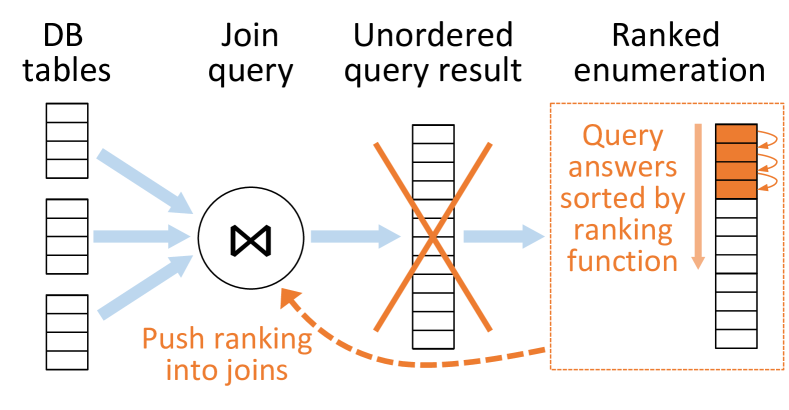
Figure 1: Enumerating the query answers in ranked order without first materializing the unordered query result. Our approach pushes sorting into the join operation so that joining and ranking are interleaved.

1 Introduction

Data analytics queries can generate large intermediate or final results, rendering data systems unresponsive. A primary culprit is the join operator, which combines data from different tables, potentially causing a combinatorial explosion in the output. Consequently, traditional join-processing techniques can become infeasible, or they simply take too long before delivering any answer to the user or to the next step in a data-processing pipeline. Work on enumeration [6, 37] addresses this by returning query answers incrementally as quickly as possible, even when the full query output is too large to compute. However, enumeration traditionally does not support a desired order (or ranking) specifying, which answers should be returned first. We thus refer to it as unranked enumeration. In practice, certain answers may be preferred over others based on some notion of importance or relevance. For instance, higher importance may be assigned to newer or more trusted data. Ranked enumeration [20, 39] therefore augments enumeration with a total-order feature over the query answers, formalized by a ranking function (e.g., expressed by an ORDER BY clause in SQL).

Database systems today follow a join-then-rank approach, i.e. they first compute all join answers and then apply the ranking (by sorting either incrementally or in batch). One way to think about the improvement we seek is that we want to “push” the ranking operator deeper into the query plan. While this resembles typical database optimizations, such as pushing projections before joins, our task turns out to be more challenging, because join and ranking operators generally do not commute. Novel algorithms are required, where joining and ranking are interleaved.

Performance Goal. How do we measure performance for such an algorithm? The top-ranked answers should be returned quickly without wasting resources on low-ranked ones, similar to classic top-$k$ queries [25]. However, in contrast to top-$k$, where “pruning” techniques based on the given number of returned answers $k$ can be leveraged, a ranked-enumeration algorithm does not know the value $k$ in advance. Instead of pruning, it can at best postpone work on lower-ranked answers, providing guarantees no matter how many answers are eventually returned. We are thus interested in the Time-To-$k$, or $\mathrm{TT}(k)$, for any possible value of $k$. This gave rise to the “any-$k$” label, quasi an “anytime top-$k$” algorithm [14, 48, 49].

Note that a stricter and popular [6, 24, 34, 37] measure of performance involves combining preprocessing time (i.e., $\mathrm{TT}(1)$) with the worst-case delay between answers (i.e., the maximum inter-arrival time). However, lowering the worst-case delay may have no practical benefit if it does not also improve $\mathrm{TT}(k)$ [41]. Adopting $\mathrm{TT}(k)$ allows for situations where a spike in delay is offset by shorter delays in previous iterations. An established example where this difference occurs is incremental QuickSort [36] which guarantees $\mathrm{TT}(k)={\mathcal{O}}(n+k\log k)$, but has a linear worst-case delay between answers.

  SELECT Cit1.PaperID, Cit2.PaperID, Cit3.PaperID,
         Cit3.CitedPaperID, Cit1.InflWeight +
         Cit2.InflWeight + Cit3.InflWeight AS Weight
  FROM Cit Cit1, Cit Cit2, Cit Cit3
  WHERE Cit1.CitedPaperID = Cit2.PaperID AND
        Cit2.CitedPaperID = Cit3.PaperID
  ORDER BY Weight

Figure 2: SQL query for ranking chains of highly influential citations.

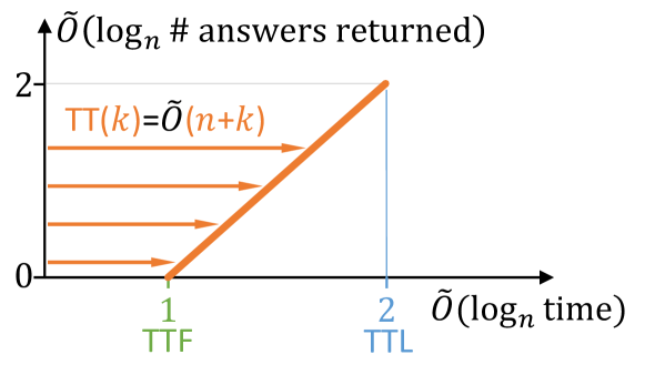
Figure 3: Ranked enumeration guarantees for the query of Figure 2: The first answer (TTF for Time-To-First) is returned in $\tilde{{\mathcal{O}}}(n)$ and the last answer (TTL for Time-To-Last) in $\tilde{{\mathcal{O}}}(n^{2})$.

An Example. Consider a bibliography dataset that stores the influence of research papers on later papers that cite them. Each tuple in relation $\mathsf{Cit}(\mathrm{PaperID},\allowbreak\mathrm{CitedPaperID},\allowbreak\mathrm{InflWeight})$ states that a paper with ID $\mathrm{CitedPaperID}$ influenced a later paper $\mathrm{PaperID}$ with a numerical weight $\mathrm{InflWeight}$. For the sake of the example, assume that the influence weight has been precomputed by some prediction technique and takes on an integer value in range [1, 10], with 1 being the most influential. To extract chains of highly influential citations, we can write the join query

$$\mathsf{Cit}(p_{1},p_{2},s_{1})\,,\,\mathsf{Cit}(p_{2},p_{3},s_{2})\,,\,\mathsf{Cit}(p_{3},p_{4},s_{3})$$

and order its answers in ascending sequence of the SUM $s_{1}+s_{2}+s_{3}$. For readers unfamiliar with Datalog, note that relation $\mathsf{Cit}$ appears three times to indicate a self-join (which requires renaming to $\mathsf{Cit1},\mathsf{Cit2},\mathsf{Cit3}$ in SQL as shown in Figure 2) and that a variable like $p_{2}$ appearing more than once indicates an equi-join between the corresponding columns (i.e., $\mathsf{Cit1}.p_{2}=\mathsf{Cit2}.p_{2}$). How fast can ranked enumeration be here? The entire query output can have size $n^{2}$ in the worst case [5]. On the other hand, simply checking if any query answer exists (called the Boolean query) takes $\Theta(n)$ [50]. Ranked enumeration aims to cover the continuum between those two with $\mathrm{TT}(k)=\tilde{{\mathcal{O}}}(n+k)$, as shown in Figure 3. The $\tilde{{\mathcal{O}}}$ notation abstracts away logarithmic factors in $n$ and $k$ introduced by join indexes or sorting (by $s_{1}+s_{2}+s_{3}$).

Prioritizing Computation. To build intuition, let us first consider how unranked enumeration works. If we were to follow a standard table-at-a-time approach, we would start by joining $\mathsf{Cit1}\bowtie\mathsf{Cit2}$. This is a costly bulk computation of time complexity $\tilde{{\mathcal{O}}}(n^{2})$. However, it would not yet produce a single query answer because table $\mathsf{Cit3}$ has not been checked. To produce answers as quickly as possible, we need to be more careful in where we spend resources and prioritize differently. Instead of a table-at-a-time, a tuple-at-a-time approach is needed. We start with only one tuple from $\mathsf{Cit1}$, look up the matches in $\mathsf{Cit2}$, pick one, and then look up the $\mathsf{Cit3}$ matches to produce one answer. This strategy can be implemented using a pipelined execution in a database system. The standard unranked enumeration algorithm [6] achieves $\tilde{{\mathcal{O}}}(n+k)$ by following such an approach, preceded by a $\tilde{{\mathcal{O}}}(n)$-time semi-join reduction [50], which removes “dangling” tuples that do not contribute to the final output.

Ranked enumeration appears more challenging because additional prioritization is required to avoid low-ranking query answers. Interestingly, a more careful look at the unranked enumeration algorithm [6] reveals that, with appropriate sorting of the input relations, the output naturally follows a lexicographic order. A lexicographic order is defined by a sequence of variables, such as $s_{1}\parbox{8.5359pt}{ \leavevmode\hbox to9.39pt{\vbox to5.2pt{\text{[drawing]}}}}s_{2}\parbox{8.5359pt}{ \leavevmode\hbox to7.51pt{\vbox to5.2pt{\text{[drawing]}}}}s_{3}$. It means that the answers are first ordered by variable $s_{1}$, then by $s_{2}$, and then by $s_{3}$ (ORDER BY Cit1.InflWeight, Cit2.InflWeight, Cit3.InflWeight in SQL). This heavily prioritizes the weight of the first citation in the chain; a chain with weights $1\parbox{8.5359pt}{ \leavevmode\hbox to7.51pt{\vbox to5.2pt{\text{[drawing]}}}}10\parbox{8.5359pt}{ \leavevmode\hbox to7.51pt{\vbox to5.2pt{\text{[drawing]}}}}10$ would be ranked higher than a chain with weights $2\parbox{8.5359pt}{ \leavevmode\hbox to7.51pt{\vbox to5.2pt{\text{[drawing]}}}}1\parbox{8.5359pt}{ \leavevmode\hbox to7.51pt{\vbox to5.2pt{\text{[drawing]}}}}1$. The enumeration algorithm of Bagan et al. [6] is capable of producing such an order, granted that we first sort each copy of $\mathsf{Citi}$ by $\mathrm{InflWeight}$.

But what if a different order that is “inconvenient” for the algorithm is required? As we will discuss in more detail, certain lexicographic orders, such as $s_{2}\parbox{8.5359pt}{ \leavevmode\hbox to7.51pt{\vbox to5.2pt{\text{[drawing]}}}}s_{1}\parbox{8.5359pt}{ \leavevmode\hbox to7.51pt{\vbox to5.2pt{\text{[drawing]}}}}s_{3}$ cannot be achieved by this approach. Moreover, for SUM ranking, the situation is more difficult because a high-ranking tuple in $\mathsf{Cit1}$ might only join with low-ranking tuples in $\mathsf{Cit2}$ and $\mathsf{Cit3}$, leading to low-ranking answers in aggregate. Addressing this requires a stronger form of prioritization that incorporates lookahead information about tuples and weights that come later in the query plan.

Any-$k$ Algorithms. We have developed and implemented algorithms that achieve $\mathrm{TT}(k)=\tilde{{\mathcal{O}}}(n+k)$ for acyclic join queries and subset-monotone ranking functions [39, 41]. These include all lexicographic orders, SUM, as well as MIN and MAX. In our example, the first $k={\mathcal{O}}(1)$ answers are obtained after only $\tilde{{\mathcal{O}}}(n)$, and—if the enumeration is carried out to the end—the last answer in $\tilde{{\mathcal{O}}}(n^{2})$, matching the join-then-rank approach. Compared to unranked enumeration, ranking by $s_{1}+s_{2}+s_{3}$ introduces only a logarithmic factor in $k$.

Although multiple any-$k$ algorithms exist [41], their complexity differences concern logarithmic factors and treating query size as a variable that can grow arbitrarily, which may not always materialize in practice. In this article, we cater to practicality and ease of understanding, focusing on data complexity, guarantees in $\tilde{{\mathcal{O}}}$ without logarithmic factors, and on the easiest-to-understand variant. We describe the algorithm in a straightforward way, without relying on the graph abstraction that we have previously used [39, 41] to highlight the connection to earlier work on shortest path enumeration [26, 29].

Organization. The rest of this article is organized as follows. Section 2 introduces necessary concepts and notation. Section 3 presents a simple algorithm that works for certain lexicographic orders and explores which lexicographic orders are achievable with this algorithm. Section 4 takes on the harder case of SUM. Section 5 discusses several extensions that generalize the approach to more expressive queries and ranking functions. Section 6 concludes and provides directions for future work.

2 Basic Concepts

We focus on Select-Project-Join queries, which we formally define in the usual way as Conjunctive Queries. Throughout the article, we use $[m]$ to denote the set of integers $\{1,\ldots,m\}$.

Database. A database $D$ is a set of finite relations $\{R_{1},\ldots,R_{m}\}$, where each $R_{i}$ for $i\in[m]$ has arity $\texttt{ar}(R)$ (i.e., $\texttt{ar}(R)$ attributes or columns) and draws values from a fixed infinite domain ${\mathtt{dom}}$, (i.e., $R_{i}\subseteq{\mathtt{dom}}^{\texttt{ar}(R_{i})}$). The size of the database $n$ is the number of tuples across all relations.

Query. In Datalog, a Conjunctive Query (CQ) $Q$ is an expression $Q(\bm{\mathbf{Y}})\allowbreak{\,:\!\!-\,}\allowbreak R_{1}(\bm{\mathbf{V_{1}}}),\allowbreak\ldots,\allowbreak R_{\ell}(\bm{\mathbf{V_{\ell}}})$, where each $\bm{\mathbf{V}}_{i}$ for $i\in[\ell]$ is a list of either variables (representing database attributes) or constants from ${\mathtt{dom}}$ (encoding selection). Each atom $R_{i}(\bm{\mathbf{V_{i}}})$ refers to a (not necessarily distinct) database relation with $|\bm{\mathbf{V_{i}}}|$ attributes. If $\bm{\mathbf{X}}$ is the set of all distinct variables appearing in all lists $\bm{\mathbf{V}}_{i}$ for $i\in[\ell]$, then the variables $\bm{\mathbf{Y}}$ (representing output attributes) need to be a subset of $\bm{\mathbf{X}}$ and are called free. A Join Query (JQ) is a special case of a CQ where all variables are free (i.e., $\bm{\mathbf{Y}}=\bm{\mathbf{X}}$). Multiple atoms are allowed to refer to the same relation, which we call a self-join. The query size, measured by the number of symbols in the query, is assumed to be ${\mathcal{O}}(1)$. This is often referred to as data complexity [46] and it is relevant in practice because while new data may be collected, the query size does not typically grow unboundedly.

Queries are evaluated over a database $D$ and produce a result $Q(D)$. A query answer or output tuple is an element $q\in Q(D)$. The occurrence of the same variable in different atoms encodes an equi-join condition, implying equality between the corresponding attributes. A typical preprocessing step for all algorithms is to (1) remove self-joins from the query by copying database tables and (2) remove selections on individual relations (like $R(x,1)$ or $R(x,x)$) by filtering. These operations take ${\mathcal{O}}(n)$ and can be ignored because the cost is asymptotically the same as reading the database once. Afterwards, a naive evaluation strategy to compute $Q(D)$ (which helps to understand the query semantics) is to ($i$) materialize the Cartesian product of the $\ell$ relations, ($ii$) select tuples that satisfy the equi-joins, and ($iii$) project on the $\bm{\mathbf{Y}}$ attributes.

Acyclicity. A CQ is (alpha-)acyclic [16] if it admits a join tree. A join tree is a rooted tree whose nodes are the query atoms and for each variable $x$, all tree nodes containing $x$ form a connected subtree. The acyclicity of a CQ can be tested, and a corresponding join tree can be constructed, in linear time in the query size [38].

Ranking. Ranked enumeration assumes a user-specified ranking function that orders the query answers $Q(D)$ by mapping them to a domain $W$ equipped with a total order $\preceq$. Ties are broken arbitrarily. Given a query $Q$, a lexicographic order $L$ is a sequence of query variables $x_{1}\parbox{8.5359pt}{ \leavevmode\hbox to7.51pt{\vbox to5.2pt{\text{[drawing]}}}}x_{2}\parbox{8.5359pt}{ \leavevmode\hbox to7.51pt{\vbox to5.2pt{\text{[drawing]}}}}\ldots$, implying that the answers are first compared by the values of $x_{1}$, and if tied by the values of $x_{2}$, and so on. A partial lexicographic order contains a strict subset of the query variables. Another case is SUM, given by an expression $f_{1}(x_{1})\allowbreak+\allowbreak f_{2}(x_{2})\allowbreak+\allowbreak\ldots$, where $f_{1},\allowbreak f_{2},\allowbreak\ldots$ can be arbitrary, ${\mathcal{O}}(1)$-computable functions mapping ${\mathtt{dom}}$ to ${\mathbb{R}}$.

3 Enumeration by Lexicographic Order

We begin with the lexicographic orders that can be produced as a by-product of the standard “unranked” enumeration algorithm through a minor extension (i.e., pre-sorting all input relations according to the lexicographic order). Although various descriptions of this algorithm exist in the literature using different abstractions [6, 11, 34, 37], it is often overlooked that it can easily produce query answers according to certain lexicographic orders.

We offer a detailed description that ($i$) is easy to implement and ($ii$) generalizes to SUM (Section 4) and other orders. We focus on acyclic JQs and discuss how this restriction can be lifted in Section 5.

The algorithm consists of two phases. First, the preprocessing phase builds essential data structures such as join indexes and applies a semijoin reduction [50] to remove dangling tuples from the input relations. Then, the enumeration phase traverses the relations using the indexes to connect joining tuples. The $\tilde{{\mathcal{O}}}(n+k)$ complexity guarantee for $\mathrm{TT}(k)$ hinges on the semijoin filtering, which eliminates “dead-ends” by ensuring that every partial query answer—generated by joining tuples from a subset of relations—can be extended to a complete query answer. We will detail both phases in Sections 3.1 and 3.2, then examine, which lexicographic orders can be supported by this algorithm in Section 3.3.

As a guiding example, we use the query $R(x_{1},x_{2}),\allowbreak S(x_{1},x_{3}),\allowbreak T(x_{2},x_{4}),\allowbreak U(x_{4},x_{5})$ and show how to achieve the order $x_{1}\parbox{8.5359pt}{ \leavevmode\hbox to7.51pt{\vbox to5.2pt{\text{[drawing]}}}}x_{2}\parbox{8.5359pt}{ \leavevmode\hbox to7.51pt{\vbox to5.2pt{\text{[drawing]}}}}x_{3}\parbox{8.5359pt}{ \leavevmode\hbox to7.51pt{\vbox to5.2pt{\text{[drawing]}}}}x_{4}\parbox{8.5359pt}{ \leavevmode\hbox to7.51pt{\vbox to5.2pt{\text{[drawing]}}}}x_{5}$. An example database is shown in Figure 4.

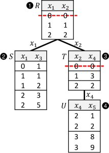
Figure 4: An example database for the join query $R(x_{1},x_{2}),S(x_{1},x_{3}),T(x_{2},x_{4}),U(x_{4},x_{5})$. The relations are organized in a join tree. Red marks indicate tuples removed by the semijoin reduction. Also shown are shared variables between child-parent pairs and the relation ordering rel used by the lexicographic enumeration algorithm.

3.1 Bottom-up Preprocessing Phase

Join Order. The preprocessing phase starts by organizing the relations in a (rooted) join tree $\mathcal{T}$. Unlike a database query plan, a join tree does not fully specify the join order. It only determines that a parent relation must be processed before its children (also called a topological sort). Hence any order that respects this constraint can be followed by the enumeration algorithm. Let function rel denote such an order, i.e., it maps the integers $[\ell]$ to database relations, where $\ell$ is the number of relations. In our example, we have $\texttt{rel}(1)\!=\!R,\texttt{rel}(2)\!=\!S,\texttt{rel}(3)\!=\!T,\texttt{rel}(4)\!=\!U$ (see Fig. 4). This means that relation $S$ will always be visited before relation $T$ during enumeration. To encode the tree structure, we refer to the parent of the $r$-th relation in the order as $\texttt{pr}(r)$, for $r\in[2,\ell]$.

Join Indexes. Next, we build join indexes, e.g., B-trees or hash indexes, allowing us to find matching tuples efficiently. We abstract an index as a function $\textrm{JoinIndex}_{R\rightarrow S}$, which, given a tuple $t\in R$, returns a list $M$ of $S$ tuples that agree with $t$ on the join attributes between $R$ and $S$ (i.e., the common variables between the atoms). To achieve the desired $\mathrm{TT}(k)$ guarantees, the index must be built in $\tilde{{\mathcal{O}}}(n)$ with lookups in $\tilde{{\mathcal{O}}}(1)$ (not including the time it takes to read $M$). We construct one index for each parent-child pair in the join tree, i.e., $\textrm{JoinIndex}_{R\rightarrow S}$ based on $x_{1}$, $\textrm{JoinIndex}_{R\rightarrow T}$ based on $x_{2}$, $\textrm{JoinIndex}_{T\rightarrow U}$ based on $x_{4}$ in our example. Figure 4 shows each relation grouped by the attributes that join with the parent, i.e., the image of $\textrm{JoinIndex}_{\texttt{pr}(r)\rightarrow\texttt{rel}(r)}$ for the $r$-th relation, $r\in[2,\ell]$. The root has no grouping.

Semijoin reduction. Using the join tree and indexes, we perform a semijoin reduction exactly as in the bottom-up step of the Yannakakis algorithm [50]. The relations are traversed in reverse topological order with a semijoin applied for each parent-child pair. In our example, the semijoins are executed in the following order:

$$T=T\ltimes U,\;\;R=R\ltimes T,\;\;R=R\ltimes S$$

This step is crucial for our desired complexity guarantee. To understand why, consider tuple $R(0,0)$, for which there are matching tuples in $S$ and $T$, but none in $U$. Consequently, the time processing $R(0,0)$ is wasted, without producing an output tuple. With sufficiently many such “dangling” tuples, the time between consecutive answers would grow to exceed $\mathrm{TT}(k)=\tilde{{\mathcal{O}}}(n+k)$. The semijoin reduction prevents this by removing dangling tuples like $R(0,0)$ and $T(0,0)$. Notice that $S(0,1)$ is dangling, but not removed. Removing all dangling tuples would require a full reduction [9, 13], which is not necessary for the enumeration algorithm. It is easy to show that any remaining dangling tuples will never be accessed by top-down traversals.

Algorithm 1 presents the semijoin reduction expressed in a way that easily generalizes to support other orders, as we will see in Section 4. Specifically, it can be viewed as message passing at the tuple level: Each tuple pulls “messages” from joining tuples in the children relations, determines its own state based on the messages, and later passes a message up the tree. The “message” here is a Boolean value that indicates whether matching tuples exist in the subtree. If the aggregated message from at least one of the children relations is “False”, then the tuple is removed and a “False” message is propagated upwards. Note that parents are “pulling” instead of children “pushing” messages so that we can use the parent-to-child join indexes that we anyway need in the enumeration phase. The algorithm employs memoization for the aggregated message of a join group (Algorithm 1), since multiple tuples in the parent relation may access it. This is important in order to guarantee linear time.

Sorting. When we build a join index, we sort its entries (i.e., the tuples within the same join group) by the same lexicographic order. In the example, the entries of $\textrm{JoinIndex}_{R\rightarrow S}$ are sorted by $x_{1}\parbox{8.5359pt}{ \leavevmode\hbox to7.51pt{\vbox to5.2pt{\text{[drawing]}}}}x_{3}$, the entries of $\textrm{JoinIndex}_{R\rightarrow T}$ by $x_{2}\parbox{8.5359pt}{ \leavevmode\hbox to7.51pt{\vbox to5.2pt{\text{[drawing]}}}}x_{4}$, and so on. The join index is built after reducing a relation with messages from its children, and sorted thereafter. The tuples of the root relation are considered to belong to the same join group (as if a parent relation with an empty set of join variables to group-by existed) and are also sorted. Slightly abusing the notation, we treat a relation as a sorted list of tuples; e.g., $R[1]$ denotes the first tuple of $R$.

1

Input: acyclic JQ $Q$ (without self-joins), database $D$, join tree $\mathcal{T}$, lexicographic order $L$, relation ordering rel consistent with $\mathcal{T}$

2 Output: reduced and sorted database $D^{\prime}$, $\textrm{JoinIndex}_{R\rightarrow S}$ for each parent $R$ and child $S$ in $\mathcal{T}$

3

4Initialize $\texttt{val}(t)=\texttt{True}$ for all tuples $t$ of all relations

5

6//Process relations in reverse rel order (bottom-up in $\mathcal{T}$)

7for $i=\ell$ down to 2  do

8       relation $S=\texttt{rel}[i]$; relation $R=\texttt{pr}(S)$

9      //Relation $S$ has been reduced in a previous iteration

10      (or is a leaf)

11      

12      Construct $\textrm{JoinIndex}_{R\rightarrow S}$ on shared attributes

13      

14      Sort $\textrm{JoinIndex}_{R\rightarrow S}$ entries by $L$

15      

16      for tuple $t\in R$ do

17             $M=\textrm{JoinIndex}_{R\rightarrow S}(t)$

18             //Memoization: $\texttt{val}(M)$ is reused

19             if $\texttt{val}(M)$ not already computed then

20                   $\texttt{val}(M)=\texttt{False}\lor\bigvee_{t^{\prime}\in M}\texttt{val}(t^{\prime})$

21                  

22            $\texttt{val}(t)=\texttt{val}(t)\wedge\texttt{val}(M)$

23             if not $\texttt{val}(t)$ then remove $t$ from $R$ in $D$

24            

25Sort the root $R$ by $L$

26

27return $D$, $\textrm{JoinIndex}_{R\rightarrow S}$ for all $(R,S)\in\mathcal{T}$

28

Algorithm 1 Preprocessing for lexicographic enumeration (Section 3.1).

3.2 Top-down Enumeration Phase

While the semijoin reduction proceeds bottom-up in the opposite direction of relation order rel (Algorithm 1), the enumeration phase traverses the relations top-down. We start with tuple $R[1]=R(1,1)$ and, through the join indexes, find the first match in every relation, yielding the first query answer $(1,1,1,3,8)$. In the second iteration, we proceed with the matches from the last relation, i.e., tuple $(3,9)$ from $U$, obtaining $(1,1,1,3,9)$. This exhausts all matches in $U$, therefore in the third iteration the algorithm backtracks to the next match in preceding relation $T$. Since no second match exists in $T$, we backtrack once again to $S$, encountering $(1,2)$ there. With $(1,1,2)$ as a partial answer, the algorithm proceeds forward to $T,U$ to obtain $(1,1,2,3,8)$. The process continues analogously, returning answers $(1,1,2,3,9)$, $(2,2,3,2,1)$, etc.

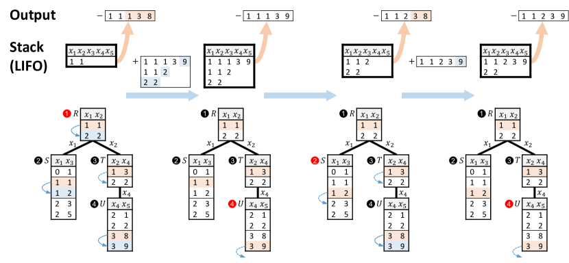
Figure 5: Enumeration steps for the first 4 answers by Algorithm 2 described in Section 3. The stack, shown on top, pops a partial answer, which is extended with the first matching tuples (in orange color) and moved to the output in each iteration. Starting from the last relation for which a tuple is in the partial answer (in red color), we check if a “next” tuple in the same join group exists (in blue color) and push a new answer to the stack. Dashed arrows indicate that there is no next.

This enumeration can be implemented recursively, akin to a standard depth-first search (DFS). Equivalently, we implement it with a stack of partial query answers (LIFO), which tracks the current frontier. A partial answer contains matched tuples from only a subset of the relations. When a partial answer is popped from the stack and we extend it into a complete answer, alternatives that use the next available tuple are pushed back onto the stack, starting from the current relation. The extension of a partial answer always selects the first matching tuple following the relation order. This is illustrated in Figure 5. Notice that when the second answer $(1,1,1,3,9)$ is popped, the current relation is $\texttt{rel}(4)=U$, with $R(1,1)$, $S(1,1)$, and $T(1,3)$ from the earlier relations considered fixed (so we do not generate new answers from those relations). In fact, $(1,1,2)$ is already on the stack from the previous iteration. This logic ensures that we enumerate each query answer exactly once. For the time complexity, note that we visit each relation at most once in each iteration, thus the cost per iteration is $\tilde{{\mathcal{O}}}(1)$ because query size is treated as a constant.

The LIFO nature of the stack is essential for achieving the lexicographic order. For instance, new answers that replace $U$-tuples (thus, change only the $x_{5}$ value) are always popped before answers that replace tuples in $R$, $S$, or $T$. In the following, we discuss the achievable orders in more detail.

1

Input: acyclic JQ $Q$, database $D$, lexicographic order $L$ without disruptive trio

Output: Ranked enumeration of $Q(D)$ in $L$ order

2

3Remove self-joins from $Q$ by copying the corresponding relations and renaming them in both $D$ and $Q$

4

5Construct an $L$-consistent join tree $\mathcal{T}$ of $Q$ with $L$-consistent relation order given by $\texttt{rel}(i),i\in[\ell]$

6

7Preprocess($Q$, $D$, $\mathcal{T}$, $L$, rel) (Algorithm 1)

8

9//A partial answer in the stack is represented as a list of input tuples together with their positions in the corresponding join groups (to easily get the next)

10 Initialize stack $\mathcal{S}$ with element $[(t_{1},1)]$ where $t_{1}=R[1]$ and $R$ is the root of $\mathcal{T}$

11

12repeat

13      

14      //Pop a partial answer ($1\leq r\leq|\mathcal{T}|$), which also contains the positions $j_{i}$ for each tuple $t_{i}$

15       $s=\mathcal{S}.\mathrm{pop}()$; $[(t_{1},j_{1}),\ldots,(t_{r},j_{r})]=s$

16      

17      //Look up matches in $r$-th relation

18       $M_{r}=\textrm{JoinIndex}_{\texttt{pr}(r)\rightarrow\texttt{rel}(r)}(t_{\texttt{pr}(r)})$

19      

20      //Push partial answer with next tuple of $r$-th relation. It exists if $j_{r}$ is not the last position in the group $M_{r}$

21       if $|M_{r}|\geq j_{r}+1$ then

22             $s^{\prime}=s.\mathrm{copy}().\mathrm{replaceLast}((M_{r}[j_{r}+1],j_{r}+1))$

23             $\mathcal{S}.\mathrm{push}(s^{\prime})$

24            

25      //Range over the remaining relations

26       for $i$ from $r+1$ to $|\mathcal{T}|$ do

27            

28            //Look up matches in $i$-th relation

29             $M_{i}=\textrm{JoinIndex}_{\texttt{pr}(i)\rightarrow\texttt{rel}(i)}(t_{\texttt{pr}(i)})$

30            

31            //Extend partial answer with first tuple in matches of $i$-th relation

32             $t_{i}=M_{i}[1]$; $s.\mathrm{append}((t_{i},1))$

33            

34            //$s$ is now $[(t_{1},j_{1}),\ldots,(t_{r},j_{r}),\ldots,(t_{i},1)]$

35            

36            if $|M_{i}|\geq 2$ then

37                   //Push partial answer with next tuple of $i$-th relation to stack $\mathcal{S}$

38                   $s^{\prime}=s.\mathrm{copy}().\mathrm{replaceLast}((M_{i}[2],2))$

39                   $\mathcal{S}.\mathrm{push}(s^{\prime})$

40                  

41      Merge $s$ into single tuple and output

42      

43until query is interrupted or $\mathcal{S}$ is empty

Algorithm 2 Ranked enumeration for lexicographic orders without disruptive trios

3.3 Supported Lexicographic Orders

Different lexicographic orders can be achieved by different sortings of the individual relations. For example, if we sort $R$ by $x_{2}\parbox{8.5359pt}{ \leavevmode\hbox to7.51pt{\vbox to5.2pt{\text{[drawing]}}}}x_{1}$, we can achieve the order $x_{2}\parbox{8.5359pt}{ \leavevmode\hbox to7.51pt{\vbox to5.2pt{\text{[drawing]}}}}x_{1}\parbox{8.5359pt}{ \leavevmode\hbox to7.51pt{\vbox to5.2pt{\text{[drawing]}}}}x_{3}\parbox{8.5359pt}{ \leavevmode\hbox to7.51pt{\vbox to5.2pt{\text{[drawing]}}}}x_{4}\parbox{8.5359pt}{ \leavevmode\hbox to7.51pt{\vbox to5.2pt{\text{[drawing]}}}}x_{5}$ without any other change in the algorithm. Some other orders can be achieved by additionally selecting a different topological sort on the join tree. With $[R,T,U,S]$ instead of $[R,S,T,U]$, we can achieve $x_{1}\parbox{8.5359pt}{ \leavevmode\hbox to7.51pt{\vbox to5.2pt{\text{[drawing]}}}}x_{2}\parbox{8.5359pt}{ \leavevmode\hbox to7.51pt{\vbox to5.2pt{\text{[drawing]}}}}x_{4}\parbox{8.5359pt}{ \leavevmode\hbox to7.51pt{\vbox to5.2pt{\text{[drawing]}}}}x_{5}\parbox{8.5359pt}{ \leavevmode\hbox to7.51pt{\vbox to5.2pt{\text{[drawing]}}}}x_{3}$. However, certain lexicographic orders cannot be achieved by this algorithm. Brault-Baron [15] identified a sufficient condition, which was later termed a disruptive trio [18] and shown to be necessary for other problems related to enumeration. (We discuss this in more detail in Section 6.)

Definition (Disruptive Trio)

For a CQ $Q$ and lexicographic order $L$, three variables $x_{1},x_{2},x_{3}$ from $L$ with relative order $x_{1}\parbox{8.5359pt}{ \leavevmode\hbox to7.51pt{\vbox to5.2pt{\text{[drawing]}}}}x_{2}\parbox{8.5359pt}{ \leavevmode\hbox to7.51pt{\vbox to5.2pt{\text{[drawing]}}}}x_{3}$ form a disruptive trio if $x_{1}$ and $x_{2}$ are not neighbors (i.e., they do not appear together in a $Q$ atom), but $x_{3}$ is a neighbor of both $x_{1}$ and $x_{2}$.

In our example, $x_{1},x_{4},x_{2}$ form a disruptive trio if $L$ is $x_{1}\parbox{8.5359pt}{ \leavevmode\hbox to7.51pt{\vbox to5.2pt{\text{[drawing]}}}}x_{4}\parbox{8.5359pt}{ \leavevmode\hbox to7.51pt{\vbox to5.2pt{\text{[drawing]}}}}x_{2}$ or even $x_{1}\parbox{8.5359pt}{ \leavevmode\hbox to7.51pt{\vbox to5.2pt{\text{[drawing]}}}}x_{3}\parbox{8.5359pt}{ \leavevmode\hbox to7.51pt{\vbox to5.2pt{\text{[drawing]}}}}x_{4}\parbox{8.5359pt}{ \leavevmode\hbox to7.51pt{\vbox to5.2pt{\text{[drawing]}}}}x_{5}\parbox{8.5359pt}{ \leavevmode\hbox to7.51pt{\vbox to5.2pt{\text{[drawing]}}}}x_{2}$. Intuitively, during the enumeration, we cannot transition from $R$ to $T$ without fixing $x_{1},x_{2}$ before $x_{4}$, which is inconsistent with the order $L$.

Brault-Baron showed that for lexicographic orders containing all free variables, the absence of a disruptive trio is equivalent to $L$ being a reverse alpha elimination order [[]Theorem 15]brault13thesis, and for partial lexicographic orders, it is equivalent to the lexicographic order being consistent with (or, in other words, a restriction of) a reverse alpha elimination order. An alpha elimination order is an ordering of the variables that guides the join tree construction [16]. If variable $y$ follows variable $x$ in the elimination order, then in the resulting join tree, $y$ will never appear without $x$ in any ancestor of a node that contains $x$. This guarantees that there exists a relation ordering rel such that the $L$ variables are encountered in the desired sequence. We call such an ordering of the relations, and its corresponding join tree, $L$-consistent.

If a desired lexicographic order has no disruptive trio, then we can find an $L$-consistent join tree and an $L$-consistent ordering of the relations to use with the enumeration algorithm discussed above.

Theorem 1 (LEX)

Let $Q$ be an acyclic join query over database $D$ and $L$ a lexicographic order of the variables in $Q$. If $L$ does not contain a disruptive trio, then ranked enumeration of $Q(D)$ by $L$ can be achieved with $\mathrm{TT}(k)=\tilde{{\mathcal{O}}}(n+k)$.

Algorithm 2 shows the pseudocode. After the preprocessing phase, a loop returns query answers iteratively by popping and pushing from the stack. Notice that, for each answer, we keep track of the positions $j_{1},\ldots,j_{\ell}$ of the tuples within the corresponding join group. This allows us to quickly access the next tuple in the group when constructing new answers (in Algorithms 2 and 2).

What about the lexicographic orders that contain disruptive trios? Algorithm 2 does not apply because there is no join tree that can match the order. For these orders, as well as SUM, we need a different strategy. Lexicographic orders with disruptive trios can in fact be reduced to a SUM-ordering problem by assigning the appropriate variable weights: If all relations have cardinality at most $n$, we can achieve that by setting the weight of the $i^{\textrm{th}}$ value of the $j^{\textrm{th}}$ variable in the order to $i\cdot n^{|L|-1-j}$.

4 Enumeration by SUM Order

In this section, we shift focus to ranking by SUM. Let $\sum_{i=1}^{5}x_{i}$ (in ascending order) be the ranking function for our example query. A naive strategy is to select the best tuple from each relation based on its individual weight. For instance, using the same join tree as before, we could start with $R(1,1)$ since it has the lowest weight $1+1=2$ within $R$. However, this strategy is not guaranteed to find the top answers, at least not within the time bounds we aim for. Once we choose $R(1,1)$, we will be stuck in a region of query answers with high overall weight because of the high weights of $U(3,8)$ and $U(3,9)$, which are the only matching tuples in $U$. The true top-1 answer $(2,2,3,2,1)$ starts with $R(2,2)$, which matches with $U(2,1)$. To make the right choices in $R$, the algorithm needs “lookahead” information about later matches in relations like $U$.

Unfortunately, it is infeasible to explicitly pre-compute the “lookahead” combinations of $S,T,U$ tuples in the preprocessing phase, because that would exceed our desired $\tilde{{\mathcal{O}}}(n)$. Instead, we rely on Dynamic Programming and a factorized representation of the query output. The enumeration phase is similar to the algorithm of Section 3.2, but uses a priority queue instead of a stack in order to prioritize the candidates according to the “lookahead” information computed during preprocessing.

4.1 Bottom-up Preprocessing Phase

To prioritize the tuples that lead to the lowest total weight, we modify the semijoin reduction so that, in addition to removing dangling tuples, we also compute the best possible weight $\texttt{opt}(t)$ reachable by each tuple $t$ when joining it with other tuples in its subtree. This bottom-up computation is essentially a form of Dynamic Programming.

The algorithm is easier to present using tuple weights instead of attribute weights. We set the weights of $R$ to $x_{1}+x_{2}$, of $S$ to $x_{3}$, of $T$ to $x_{4}$ and of $U$ to $x_{5}$. Such a conversion is always possible in linear time, which means that both regimes are supported in the algorithm. We only need to be careful so that the weight of each variable is assigned to a unique relation; this can be achieved through a mapping $\mu$ that assigns each variable $x$ in the SUM to the first relation (or atom) that contains $x$ in the topological sort rel. We denote the weight of tuple $t$ by $\texttt{w}(t)$. Algorithm 3 computes $\texttt{opt}(t)$ for all tuples $t$ by aggregating the input weights using $\min$ and $+$, bottom-up in reverse rel order , as shown in Figure 6. The leaf relations set $\texttt{opt}(t)$ to be equal to $\texttt{w}(t)$. For tuple $T(2,2)$, which is in the non-leaf relation $T$, we add its own weight $2$ to the message $\min\{1,2\}$ from the joining group in $U$, hence $\texttt{opt}(T(2,2))=\!2\!+\!\min\{1,2\}=\!3$. For a relation with multiple children, we add the messages from all of them. E.g., for $R(2,2)$, we add its own weight $4$ with the message $\min\{3,5\}$ from $S$ and the message $\min\{3\}$ from $T$, hence $\texttt{opt}(R(2,2))=10$. By the end of the preprocessing step, we know the optimal weight $\texttt{opt}(t)$ for each tuple $t$, and the join index entries are sorted according to these values.

Remark 1

The fact that Algorithm 3 is so similar to the semijoin reduction in Algorithm 1 is not a coincidence. They are both instances of the FAQ framework [2] with different semirings. In particular, the aggregation operators $\vee$ and $\wedge$ from the semi-join reduction are replaced with $\min$ and $+$ in the variant for SUM. In more technical terms, the former corresponds to the Boolean semiring and the latter to the tropical semiring.

Figure 6: Bottom-up Dynamic Programming for SUM (preprocessing). Orange circles show the weights $\texttt{w}(t)$ assigned to tuples. Blue squares show the calculated minimal subtree weight $\texttt{opt}(t)$ for each tuple.

1

Input: acyclic JQ $Q$ (without self-joins), database $D$ with tuple weights, join tree $\mathcal{T}$, relation ordering rel consistent with $\mathcal{T}$

2 Output: reduced and sorted database $D^{\prime}$, $\textrm{JoinIndex}_{R\rightarrow S}$ for each parent $R$ and child $S$ in $\mathcal{T}$

3

4Initialize $\texttt{opt}(t)=\texttt{w}(t)$ for all tuples $t$ of all relations

5

6$\texttt{rel}=$ relation ordering consistent with $\mathcal{T}$

7//Process relations in reverse rel order (bottom-up in $\mathcal{T}$)

8for $i=\ell$ down to 2  do

9       relation $S=\texttt{rel}[i]$; relation $R=\texttt{pr}(S)$

10      

11      //Relation $S$ has been reduced in a previous iteration

12      (or is a leaf)

13      

14      Construct $\textrm{JoinIndex}_{R\rightarrow S}$ on shared attributes

15      

16      Sort $\textrm{JoinIndex}_{R\rightarrow S}$ entries by opt

17      

18      for tuple $t\in R$ do

19             $M=\textrm{JoinIndex}_{R\rightarrow S}(t)$

20             //Memoization: $\texttt{val}(M)$ is reused

21             if $\texttt{opt}(M)$ not already computed then

22                  

23                  $\texttt{opt}(M)=\min\{\infty,\min_{t^{\prime}\in M}\texttt{opt}(t^{\prime})$ }

24                  

25            $\texttt{opt}(t)=\texttt{opt}(t)+\texttt{opt}(M)$

26             if $\texttt{opt}(t)==\infty$ then remove $t$ from $R$ in $D$

27            

28Sort the root $R$ by opt

29

30return $D$, $\textrm{JoinIndex}_{R\rightarrow S}$ for all $(R,S)\in\mathcal{T}$

31

(Section 4.1). Changes compared to Algorithm 1 are in blue.

Algorithm 3 Preprocessing for enumeration by SUM

(Section 4.1). Changes compared to Algorithm 1 are in blue.

1

Input: acyclic JQ $Q$, database $D$, SUM order $\mathcal{W}$

Output: Ranked enumeration of $Q(D)$ in $\mathcal{W}$ order

2

3Remove self-joins from $Q$ by copying the corresponding relations and renaming them in both $D$ and $Q$

4

5 Construct a join tree $\mathcal{T}$ of $Q$ with tree-consistent relation order given by $\texttt{rel}(i),i\in[\ell]$

6

7Convert attribute weights to tuple weights

8

9Preprocess($Q$, $D$, $\mathcal{T}$, rel) (Algorithm 3)

10

11//A partial answer in the stack is represented as a list of input tuples together with their positions in the corresponding join groups (to easily get the next)

12 Initialize priority queue $\mathcal{P}$ with element $[(t_{1},1)]$ where $t_{1}=R[1]$ and $R$ is the root of $\mathcal{T}$

13

14repeat

15      

16      //Pop a partial answer ($1\leq r\leq|\mathcal{T}|$), which also contains the positions $j_{i}$ for each tuple $t_{i}$

17       $s=\mathcal{S}.\mathrm{pop}()$; $[(t_{1},j_{1}),\ldots,(t_{r},j_{r})]=s$

18      

19      //Look up matches in $r$-th relation

20       $M_{r}=\textrm{JoinIndex}_{\texttt{pr}(r)\rightarrow\texttt{rel}(r)}(t_{\texttt{pr}(r)})$

21      

22      //Push partial answer with next tuple of $r$-th relation. It exists if $j_{r}$ is not the last position in the group $M_{r}$

23      

24      if $|M_{r}|\geq j_{r}+1$ then

25             $s^{\prime}=s.\mathrm{copy}().\mathrm{replaceLast}((M_{r}[j_{r}+1],j_{r}+1))$

26             ${\leavevmode\color[rgb]{0,0,1}\mathcal{P}}.\mathrm{push}(s^{\prime})$ with priority $\texttt{prio}(s^{\prime})$

27            

28      //Range over the remaining relations

29       for $i$ from $r+1$ to $|\mathcal{T}|$ do

30            

31            //Look up matches in $i$-th relation

32             $M_{i}=\textrm{JoinIndex}_{\texttt{pr}(i)\rightarrow\texttt{rel}(i)}(t_{\texttt{pr}(i)})$

33            

34            //Extend partial answer with first tuple in matches of $i$-th relation

35             $t_{i}=M_{i}[1]$; $s.\mathrm{append}((t_{i},1))$

36            

37            //$s$ is now $[(t_{1},j_{1}),\ldots,(t_{r},j_{r}),\ldots,(t_{i},1)]$

38            

39            if $|M_{i}|\geq 2$ then

40                   //Push partial answer with next tuple of $i$-th relation to priority queue $\mathcal{P}$

41                   $s^{\prime}=s.\mathrm{copy}().\mathrm{replaceLast}((M_{i}[2],2))$

42                   ${\leavevmode\color[rgb]{0,0,1}\mathcal{P}}.\mathrm{push}(s^{\prime})$ with priority $\texttt{prio}(s^{\prime})$

43                  

44      Merge $s$ into single tuple and output

45      

46until query is interrupted or $\mathcal{P}$ is empty

Algorithm 4 Ranked enumeration for SUM orders. Changes compared to Algorithm 2 are in blue.

4.2 Top-down Enumeration Phase

As can be seen in Algorithm 4, the high-level logic of the enumeration is the same as the lexicographic enumeration of Algorithm 2. Algorithms 4 and 4 generate new query answers with the tuple in the next position in the join group, like before. However, tuples within a join group are now sorted by opt, so each answer generated is guaranteed to produce the next-best weight (among those in the same join group) when extended to a complete answer.

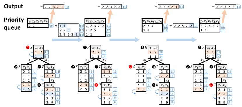
Figure 7: The example from Fig. 5 adapted with a priority queue instead of a stack to support ranked enumeration by SUM.

Another important difference is that the stack that maintains the partial answers is replaced by a priority queue $\mathcal{P}$. Initially, $\mathcal{P}$ only contains a partial answer with $R[1]=R(2,2)$, producing the top-1 answer $(2,2,3,2,1)$ with weight $\texttt{opt}(R(2,2))=10$. The second iteration has 3 candidates in $\mathcal{P}$: $(1,1)$, $(2,2,5)$ and $(2,2,3,2,2)$. The priority of each candidate $s$, denoted by $\texttt{prio}(s)$ is the weight of the answer we will obtain if we fully extend it. We compute it before inserting it into $\mathcal{P}$; we can either prematurily extend it into a full answer, or we can subtract from the previous answer the weight of the subtree that was removed and add the weight of the new subtree. For example, for $(2,2,5)$, we can subtract the weight of the subtree rooted at $S(2,3)$ and add the new weight $\texttt{opt}(S(2,5))$ to the weight of the answer of the previous iteration, yielding $10-3+5=12$. Based on the priorities, $(2,2,3,2,2)$ with priority $11$ will be the winner in the second iteration, and the enumeration continues accordingly. Figure 7 depicts the process.

The size of the priority queue $\mathcal{P}$ is at most $k\ell$, since we push at most $\ell$ candidates in each iteration. Hence, the time of each iteration now includes a logarithmic cost for priority-queue operations (instead of the earlier constant one for stack accesses). However, if we ignore logarithmic factors, the $\mathrm{TT}(k)$ complexity remains the same as in Theorem 1.

Theorem 2 (SUM)

Let $Q$ be an acyclic join query over database $D$ and $\mathcal{W}$ a SUM ranking function. Ranked enumeration of $Q(D)$ by $\mathcal{W}$ can be achieved with $\mathrm{TT}(k)=\tilde{{\mathcal{O}}}(n+k)$.

4.3 Experimental Results

We implemented any-$k$ (enumeration by SUM) and The code is available to use at https://github.com/northeastern-datalab/anyk-code. The experimental results from PVLDB’20 [39] and PVLDB’21 [42] have been independently reproduced.

Setup. We compare the performance of any-$k$ against JoinFirst (first computing the full result using the Yannakakis algorithm [50]), PSQL (PostgreSQL 9.5.20), System X (a commercial system), and DuckDB 0.10.1 on path queries (joining relations in a chain). We configure the database systems in order to minimize system overhead, provide them with indexes before query execution, and ensure that all input relations are cached in memory. We only test serial execution.

Results. Figure 8(a) reports ranked-enumeration behavior of any-$k$ on synthetic data, with $\mathrm{TT}(k)$ on the x-axis and $k$ on the y-axis. All the database systems follow an approach similar to JoinFirst, differing only in constant factors. The in-memory DuckDB system is the fastest, but by the time it returns the first answer (in 3.8 sec), any-$k$ has already returned almost 2 million answers, and the first one in 66msec. Figure 8(b) shows the scalability on a Bitcoin network, where weighted edges represent the degree of trust between users. To control data size on the x-axis, we retain edges between users whose IDs are below a certain threshold. For this experiment we fix $k\!=\!10^{3}$. JoinFirst runs out of memory as the data size increases, while the database systems are outperformed by more than 2 orders of magnitude on the full dataset. Increasing the number of joins, as shown in Figure 8(c) has an even more dramatic effect. The running time of any-$k$ stays below 1 second even for 10 joining relations, while the other approaches either time out or run out of memory with 5 or more relations.

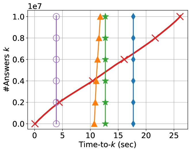
(a) 4-Path Synthetic
(varying $k$)

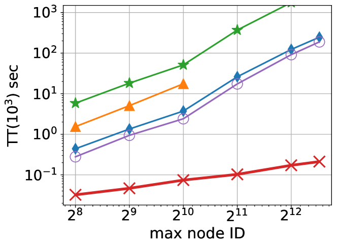
(b) 4-Path Bitcoin
(varying data size)

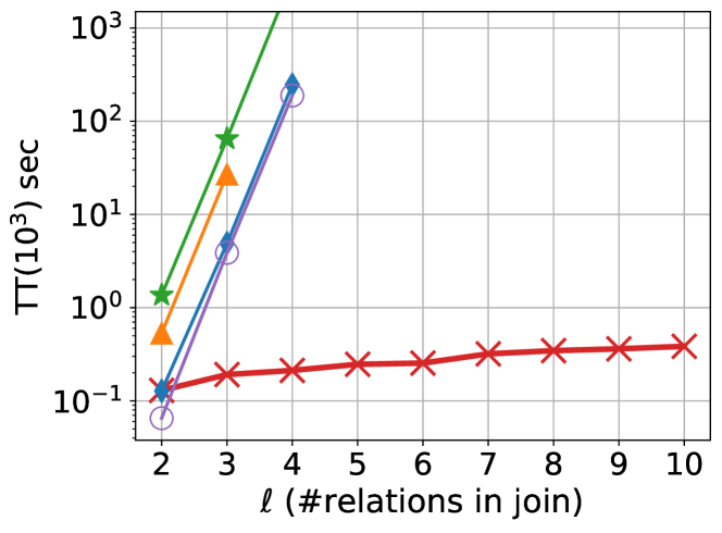
(c) $\ell$-Path Bitcoin
(varying query size)

Figure 8: Experimental results comparing any-$k$ against the join-then-rank approach (JoinFirst) and 3 database systems. Any-$k$ returns the top answer in 66 msec, whereas DuckDB needs 3.8 sec (a). As the data size or the number of joins increase (b,c), alternatives quickly time out.

5 Extensions

We consider a number of extensions of the algorithms presented so far.

5.1 General Ranking Functions

Beyond lexicographic orders and SUM, the algorithm of Section 4 can be used with any ranking function that obeys a property called subset-monotonicity. Recall that a ranking function $w$ maps the query answers to a domain $W$ ordered by $\preceq$. We consider ranking functions that achieve this by aggregating (a multiset of) input weights via an aggregate function $w_{A}$. For example, $w_{A}$ is $\sum$ for SUM.

Definition (Subset-Monotonicity)

A ranking function $w$ is subset-monotone if $w_{A}(X_{1})\preceq w_{A}(X_{2})\Rightarrow w_{A}(X_{1}\uplus Y)\preceq w_{A}(X_{2}\uplus Y)$ for all $X_{1},X_{2},Y$ $\in\mathbb{N}^{W}$, where $\uplus$ is multiset union.

Intuitively, subset-monotonicity allows us to infer the ranking of complete solutions from the ranking of partial solutions. This is essentially enabling Dynamic Programming [10].

Any subset-monotone ranking function can be handled efficiently with the $\tilde{{\mathcal{O}}}(n+k)$ guarantee for acyclic queries [41]. For instance, we may choose the aggregate function to be $\max$ instead of $\sum$. Under this ranking, only the highest weight in each query answer is relevant for ordering the answers.

What about non-subset-monotone ranking functions? A negative result has been given by Deep and Koutris [20], who showed that if the ranking function is a black box, then we cannot do better than materializing the entire query output. Thus, the only guarantee we can hope for is the worst-case output of the query, given by the AGM bound [5].

5.2 CQs with Projection

So far, we have focused on join queries, yet CQs may also contain projection. Projections introduce a new challenge: even if ranked enumeration is efficient for a join query, this may not be true for projections, because we need to eliminate duplicates (under set semantics), potentially increasing $\mathrm{TT}(k)$.

Bagan et al. [6] established a dichotomy for unranked enumeration that precisely characterizes queries that admit $\mathrm{TT}(k)=\tilde{{\mathcal{O}}}(n+k)$. The negative side of the dichotomy applies only to self-join-free CQs and relies on two complexity-theoretic hypotheses: SparseBMM [11] states that two Boolean matrices $A$ and $B$, represented as lists of non-zeros, cannot be multiplied in time $m^{1+o(1)}$ where $m$ is the number of non-zeros in $A$, $B$, and $AB$. Hyperclique [1, 30] states that for every $k\geq 2$, there is no $O(n\operatorname{polylog}n)$ algorithm to decide the existence of a $(k{+}1,k)$-hyperclique in a $k$-uniform hypergraph with $n$ hyperedges, where a $(k{+}1,k)$-hyperclique is a set of $k{+}1$ vertices such that every subset of $k$ vertices forms a hyperedge, and a $k$-uniform hypergraph is one where all hyperedges contain exactly $k$ vertices. Under these assumptions, the only efficient (self-join-free) CQs are those that are free-connex. A CQ is free-connex if it is acyclic and additionally, it remains acyclic if we add an atom that contains all free variables [15].

Interestingly, that frontier of tractability for unranked enumeration turns out to be the same for ranked enumeration with subset-monotone ranking functions (modulo logarithmic factors).

Theorem 3 (Dichotomy [41])

Let $Q$ be a CQ. If $Q$ is free-connex, then ranked enumeration with an s-monotone ranking function is possible with $\mathrm{TT}(k)=\tilde{{\mathcal{O}}}(n+k)$. Otherwise, if it is also self-join-free, then it is not possible with $\mathrm{TT}(k)=\tilde{{\mathcal{O}}}(n+k)$ for any ranking function, assuming SparseBMM and Hyperclique.

For the class of acyclic but non-free-connex CQs, the dichotomy precludes the existence of an algorithm with the efficient $\tilde{{\mathcal{O}}}(n+k)$ guarantee. However, $\tilde{{\mathcal{O}}}(n\cdot k)$ is possible for subset-monotone ranking functions. This result has been established by the algorithm of Bagan et al. [6] for lexicographic orders, by Deep et al. [19] for lexicographic orders and SUM through a different algorithm, and by Kimelfeld and Sagiv [28] for all subset-monotone ranking functions through a third algorithm.

Theorem 4 (Non-free-connex [6, 19, 28])

Let $Q$ be an acyclic, non-free-connex CQ over database $D$ and $w$ a subset-monotone ranking function. Ranked enumeration of $Q(D)$ by $w$ can be achieved with $\mathrm{TT}(k)=\tilde{{\mathcal{O}}}(n\cdot k)$.

5.3 Beyond Acyclic CQs

We can apply our ranked-enumeration algorithms even to queries that are not acyclic CQs, albeit with adjusted complexity guarantees. This is possible if the query can be transformed into an acyclic and free-connex CQ, or a union of such queries. In that case, we first apply the transformation and then perform ranked enumeration on the resulting queries. To deal with a union, we maintain a top-level priority queue that retrieves the next query answer from the query with the lowest weight in each iteration. Duplicate answers introduce potential complications, but as long as the number of duplicates per answer is bounded by a constant, they can be filtered on-the-fly without increasing complexity. In general, identifying such transformations is an orthogonal research problem, and we discuss three notable cases.

Cyclic JQs. For cyclic JQs, we can employ (hyper)tree decompositions [23] to reduce them to a union of acyclic JQs. A decomposition is associated with a width parameter that captures the degree of acyclicity of the query and affects the complexity of subsequent algorithms; for a JQ with width $d$, we can achieve $\mathrm{TT}(k)=\tilde{{\mathcal{O}}}(n^{d}+k)$. The state-of-the-art width for a JQ $Q$ is the submodular width $\textsf{subw}(Q)$ [3, 31], transforming a cyclic JQ over a database of size $n$ to a union of acyclic JQs of size ${\mathcal{O}}(n^{\textsf{subw}(Q)})$, allowing ranked enumeration with $\mathrm{TT}(k)=\tilde{{\mathcal{O}}}(n^{\textsf{subw}(Q)}+k)$.

Built-in Predicates. Another case involves acyclic JQs that additionally contain built-in predicates [45] such as inequalities. For non-equalities (or “disequalities” $\neq$), we can always achieve $\mathrm{TT}(k)=\tilde{{\mathcal{O}}}(n+k)$ regardless of where the non-equalities appear in the JQ through a “color-coding” technique [35]. Abo Khamis et al. [27] showed that the same is true for a multidimensional generalization of non-equality, called a Not-All-Equal (NAE) predicate. For inequalities ($<,>$), we can successfully reduce the query to an acyclic JQ over an $\tilde{{\mathcal{O}}}(n)$ database, hence achieving $\mathrm{TT}(k)=\tilde{{\mathcal{O}}}(n+k)$, as long as the inequality predicate involves variables that appear in join-tree nodes that are adjacent [42]. This condition can be checked directly from the query structure; it is equivalent to the absence of a chordless path of length at least 4 connecting the inequality variables, in the query’s hypergraph [40].

CQs with FDs. While a CQ may be acyclic but not free-connex, or even cyclic, it may still be possible to transform it to an acyclic CQ without employing a hypertree decomposition, which generally increase the complexity. This is the case when Functional Dependencies (FDs) are present in the CQ. We can achieve $\mathrm{TT}(k)=\tilde{{\mathcal{O}}}(n+k)$ for queries whose so-called FD-extension is free-connex [17], which is also known as the closure of $Q$ [22].

6 Conclusion and Future Outlook

In this paper, we explored the problem of ranked enumeration without fully materializing the query result. We demonstrated how, for acyclic join queries, certain lexicographic orders can naturally be produced by the unranked enumeration algorithm (with an additional sorting of individual relations). However, not all orders can be handled in this straightforward way. With additional preprocessing and data structures for prioritization, we presented an extended algorithm capable of handling more complex ranking functions, including SUM. Notably, for free-connex CQs, this approach achieves $\mathrm{TT}(k)=\tilde{{\mathcal{O}}}(n+k)$ for any subset-monotone ranking function, and no other self-join-free CQ admits this guarantee (under common hypotheses). Broader classes of queries are also within the reach of the algorithm, as long as they can be efficiently reduced to a union of acyclic and free-connex CQs.

These results contribute to an extensive line of research in database theory, focused on the computational tasks that can be efficiently performed on query results without explicitly materializing them. The goal is to offer the illusion of a materialized result, while the actual operations are executed directly on the database. Beyond ranked enumeration, related tasks include aggregation [2], linear regression [33], and $k$-means clustering [32], among others. One closely related problem is direct access [18, 21, 40], which asks whether it is possible to efficiently jump to arbitrary positions in the (implicit) output array, after a preprocessing phase. Ranked enumeration is a special case of this problem, where the accessed positions are $1,2,3,\ldots$

One of the areas lacking a refined understanding for ranked enumeration is the complexity landscape for ranking functions. Although some orders are algorithmically easier to achieve than others within the subset-monotone class, their complexity is the same, modulo logarithmic factors [41]. On the other end of the spectrum, for arbitrary black-box ranking functions, no strong guarantees can be achieved. What about the space in-between? For the problem of direct access, more intriguing separations are known, even within the class of lexicographic and SUM ranking functions. Interestingly, the disruptive trio condition (Section 3.3) that describes the feasible lexicographic orders for the algorithm of Section 3 also appears as a necessary condition for the tractability of direct access [18] (assuming SparseBMM). However, in contrast to ranked enumeration, it gives a polynomial separation of lexicographic orders. Mapping out properties of ranking functions and their impact on complexity is an interesting research direction.

In a similar vein, more work is needed to understand the fundamental difficulty of ranking. For instance, are there surprising cases where ranked enumeration is harder than unranked? One avenue to approach this question is to study CQs with “long” inequalities (in contrast to the “short” inequalities of Section 5.3). For some queries, e.g., for $Q(x_{1},x_{2},x_{3},x_{4})\allowbreak{\,:\!\!-\,}\allowbreak R(x_{1},x_{2}),\allowbreak S(x_{2},x_{3}),\allowbreak T(x_{3},x_{4}),\allowbreak x_{1}<x_{4}$, it is known that unranked enumeration can be achieved with $\tilde{{\mathcal{O}}}(n+k)$ [47], yet ranked enumeration has not been studied. Another avenue is to consider different classes of circuits [4] instead of CQs in order to find such a separation.

The relationship between ranked enumeration and top-$k$ can also lead to interesting questions. Top-$k$ introduces two relaxations, the exact impact of which is not entirely clear: (1) $k$ is a small constant, and (2) $k$ is known in advance.

Finally, parallelization is a natural, but challenging, direction. The prioritization of answers required by ranked enumeration implies a degree of sequentiality in the computation, making a parallel adaptation non-obvious. On the theoretical side, the widely used MPC model [8] does not seem to be a good fit because of its batch-processing nature.

Acknowledgements. This work was supported in part by a grant from PricewaterhouseCoopers (PwC), the National Institutes of Health (NIH) under award number R01 NS091421, and by the National Science Foundation (NSF) under award numbers CAREER IIS-1762268 and IIS-1956096. Nikolaos Tziavelis was additionally supported by a Google PhD fellowship. Any opinions, findings, and conclusions or recommendations expressed in this paper are those of the authors and do not necessarily reflect the views of the funding agencies.

References

- [1] Amir Abboud and Virginia Vassilevska Williams “Popular Conjectures Imply Strong Lower Bounds for Dynamic Problems” In FOCS, 2014, pp. 434–443 DOI: 10.1109/FOCS.2014.53
- [2] Mahmoud Abo Khamis, Hung Q Ngo and Atri Rudra “FAQ: questions asked frequently” In PODS, 2016, pp. 13–28 DOI: 10.1145/2902251.2902280
- [3] Mahmoud Abo Khamis, Hung Q Ngo and Dan Suciu “What do Shannon-type Inequalities, Submodular Width, and Disjunctive Datalog have to do with one another?” In PODS, 2017, pp. 429–444 DOI: 10.1145/3034786.3056105
- [4] Antoine Amarilli, Pierre Bourhis, Florent Capelli and Mikaël Monet “Ranked Enumeration for MSO on Trees via Knowledge Compilation” In ICDT 290, 2024, pp. 25:1–25:18 DOI: 10.4230/LIPIcs.ICDT.2024.25
- [5] Albert Atserias, Martin Grohe and Dániel Marx “Size Bounds and Query Plans for Relational Joins” In SIAM J. Comput. 42.4, 2013, pp. 1737–1767 DOI: 10.1137/110859440
- [6] Guillaume Bagan, Arnaud Durand and Etienne Grandjean “On acyclic conjunctive queries and constant delay enumeration” In International Workshop on Computer Science Logic (CSL), 2007, pp. 208–222 DOI: 10.1007/978-3-540-74915-8_18
- [7] Nurzhan Bakibayev, Tomáš Kočiský, Dan Olteanu and Jakub Závodný “Aggregation and Ordering in Factorised Databases” In PVLDB 6.14 VLDB Endowment, 2013, pp. 1990–2001 DOI: 10.14778/2556549.2556579
- [8] Paul Beame, Paraschos Koutris and Dan Suciu “Communication Steps for Parallel Query Processing” In J. ACM 64.6, 2017 DOI: 10.1145/3125644
- [9] Catriel Beeri, Ronald Fagin, David Maier and Mihalis Yannakakis “On the Desirability of Acyclic Database Schemes” In J. ACM 30.3, 1983, pp. 479–513 DOI: 10.1145/2402.322389
- [10] Richard Bellman “The theory of dynamic programming” In Bull. Amer. Math. Soc. 60.6 American Mathematical Society, 1954, pp. 503–515 URL: https://projecteuclid.org:443/euclid.bams/1183519147
- [11] Christoph Berkholz, Fabian Gerhardt and Nicole Schweikardt “Constant Delay Enumeration for Conjunctive Queries: A Tutorial” In ACM SIGLOG News 7.1 New York, NY, USA: ACM, 2020, pp. 4–33 DOI: 10.1145/3385634.3385636
- [12] Christoph Berkholz and Nicole Schweikardt “Constant Delay Enumeration with FPT-Preprocessing for Conjunctive Queries of Bounded Submodular Width” In MFCS 138, LIPIcs, 2019, pp. 58:1–58:15 DOI: 10.4230/LIPIcs.MFCS.2019.58
- [13] Philip A. Bernstein and Dah-Ming W. Chiu “Using Semi-Joins to Solve Relational Queries” In J. ACM 28.1, 1981, pp. 25–40 DOI: 10.1145/322234.322238
- [14] Mark S Boddy “Anytime Problem Solving Using Dynamic Programming.” In AAAI, 1991, pp. 738–743 URL: https://dl.acm.org/doi/abs/10.5555/1865756.1865791
- [15] Johann Brault-Baron “De la pertinence de l’énumération: complexité en logiques propositionnelle et du premier ordre”, 2013 URL: https://hal.archives-ouvertes.fr/tel-01081392
- [16] Johann Brault-Baron “Hypergraph Acyclicity Revisited” In ACM Comput. Surv. 49.3 New York, NY, USA: Association for Computing Machinery, 2016 DOI: 10.1145/2983573
- [17] Nofar Carmeli and Markus Kröll “Enumeration Complexity of Conjunctive Queries with Functional Dependencies” In Theory Comput. Syst. 64.5, 2020, pp. 828–860 DOI: 10.1007/s00224-019-09937-9
- [18] Nofar Carmeli, Nikolaos Tziavelis, Wolfgang Gatterbauer, Benny Kimelfeld and Mirek Riedewald “Tractable Orders for Direct Access to Ranked Answers of Conjunctive Queries” In TODS 48.1, 2023 DOI: 10.1145/3578517
- [19] Shaleen Deep, Xiao Hu and Paraschos Koutris “Ranked Enumeration of Join Queries with Projections” In PVLDB 15.5, 2022, pp. 1024–1037 DOI: 10.14778/3510397.3510401
- [20] Shaleen Deep and Paraschos Koutris “Ranked Enumeration of Conjunctive Query Results” In ICDT 186, 2021, pp. 5:1–5:19 DOI: 10.4230/LIPIcs.ICDT.2021.5
- [21] Idan Eldar, Nofar Carmeli and Benny Kimelfeld “Direct Access for Answers to Conjunctive Queries with Aggregation” In ICDT 290, 2024, pp. 4:1–4:20 DOI: 10.4230/LIPIcs.ICDT.2024.4
- [22] Wolfgang Gatterbauer and Dan Suciu “Dissociation and propagation for approximate lifted inference with standard relational database management systems” In The VLDB Journal 26.1, 2017, pp. 5–30 DOI: 10.1007/s00778-016-0434-5
- [23] Georg Gottlob, Gianluigi Greco, Nicola Leone and Francesco Scarcello “Hypertree Decompositions: Questions and Answers” In PODS, 2016, pp. 57–74 DOI: 10.1145/2902251.2902309
- [24] Muhammad Idris, Martín Ugarte, Stijn Vansummeren, Hannes Voigt and Wolfgang Lehner “General dynamic Yannakakis: conjunctive queries with theta joins under updates” In VLDB J. 29 Springer, 2020, pp. 619–653 DOI: 10.1007/s00778-019-00590-9
- [25] Ihab F Ilyas, George Beskales and Mohamed A Soliman “A survey of top- query processing techniques in relational database systems” In ACM Computing Surveys 40.4, 2008, pp. 11 DOI: 10.1145/1391729.1391730
- [26] Víctor M Jiménez and Andrés Marzal “Computing the shortest paths: A new algorithm and an experimental comparison” In International Workshop on Algorithm Engineering (WAE), 1999, pp. 15–29 Springer DOI: 10.1007/3-540-48318-7_4
- [27] Mahmoud Abo Khamis, Hung Q. Ngo, Dan Olteanu and Dan Suciu “Boolean Tensor Decomposition for Conjunctive Queries with Negation” In ICDT, 2019, pp. 21:1–21:19 DOI: 10.4230/LIPIcs.ICDT.2019.21
- [28] Benny Kimelfeld and Yehoshua Sagiv “Incrementally Computing Ordered Answers of Acyclic Conjunctive Queries” In International Workshop on Next Generation Information Technologies and Systems (NGITS), 2006, pp. 141–152 DOI: 10.1007/11780991_13
- [29] Eugene L Lawler “A procedure for computing the k best solutions to discrete optimization problems and its application to the shortest path problem” In Management science 18.7 INFORMS, 1972, pp. 401–405 DOI: 10.1287/mnsc.18.7.401
- [30] Andrea Lincoln, Virginia Vassilevska Williams and R. Ryan Williams “Tight Hardness for Shortest Cycles and Paths in Sparse Graphs” In SODA, 2018, pp. 1236–1252 DOI: 10.1137/1.9781611975031.80
- [31] Dániel Marx “Tractable Hypergraph Properties for Constraint Satisfaction and Conjunctive Queries” In J. ACM 60.6 New York, NY, USA: ACM, 2013, pp. 42:1–42:51 DOI: 10.1145/2535926
- [32] Benjamin Moseley, Kirk Pruhs, Alireza Samadian and Yuyan Wang “Relational Algorithms for k-Means Clustering” In ICALP 198, 2021, pp. 97:1–97:21 DOI: 10.4230/LIPIcs.ICALP.2021.97
- [33] Dan Olteanu and Maximilian Schleich “Factorized databases” In SIGMOD Record 45.2 Association for Computing Machinery, 2016 DOI: 10.1145/3003665.3003667
- [34] Dan Olteanu and Jakub Závodnỳ “Size bounds for factorised representations of query results” In TODS 40.1 ACM, 2015, pp. 2 DOI: 10.1145/2656335
- [35] Christos H. Papadimitriou and Mihalis Yannakakis “On the complexity of database queries” In Journal of Computer and System Sciences 58.3, 1999, pp. 407–427 DOI: 10.1006/jcss.1999.1626
- [36] Rodrigo Paredes and Gonzalo Navarro “Optimal Incremental Sorting” In ALENEX, 2006, pp. 171–182 DOI: 10.1137/1.9781611972863.16
- [37] Luc Segoufin “Constant Delay Enumeration for Conjunctive Queries” In SIGMOD Record 44.1, 2015, pp. 10–17 DOI: 10.1145/2783888.2783894
- [38] Robert E Tarjan and Mihalis Yannakakis “Simple linear-time algorithms to test chordality of graphs, test acyclicity of hypergraphs, and selectively reduce acyclic hypergraphs” In SIAM J. Comput. 13.3 SIAM, 1984, pp. 566–579 DOI: 10.1137/0213035
- [39] Nikolaos Tziavelis, Deepak Ajwani, Wolfgang Gatterbauer, Mirek Riedewald and Xiaofeng Yang “Optimal Algorithms for Ranked Enumeration of Answers to Full Conjunctive Queries” In PVLDB 13.9, 2020, pp. 1582–1597 DOI: 10.14778/3397230.3397250
- [40] Nikolaos Tziavelis, Nofar Carmeli, Wolfgang Gatterbauer, Benny Kimelfeld and Mirek Riedewald “Efficient Computation of Quantiles over Joins” In PODS, 2023, pp. 303–315 DOI: 10.1145/3584372.3588670
- [41] Nikolaos Tziavelis, Wolfgang Gatterbauer and Mirek Riedewald “Any-k Algorithms for Enumerating Ranked Answers to Conjunctive Queries” In CoRR abs/2205.05649, 2023 URL: https://arxiv.org/abs/2205.05649
- [42] Nikolaos Tziavelis, Wolfgang Gatterbauer and Mirek Riedewald “Beyond Equi-joins: Ranking, Enumeration and Factorization” In PVLDB 14.11, 2021, pp. 2599–2612 DOI: 10.14778/3476249.3476306
- [43] Nikolaos Tziavelis, Wolfgang Gatterbauer and Mirek Riedewald “Optimal Join Algorithms Meet Top-k” In SIGMOD tutorials, 2020, pp. 2659–2665 DOI: 10.1145/3318464.3383132
- [44] Nikolaos Tziavelis, Wolfgang Gatterbauer and Mirek Riedewald “Toward Responsive DBMS: Optimal Join Algorithms, Enumeration, Factorization, Ranking, and Dynamic Programming” In ICDE tutorials, 2022 DOI: 10.1109/ICDE53745.2022.00299
- [45] Jeffrey D. Ullman “Principles of database and knowledge-base systems, Vol. I” Computer Science Press, Inc., 1988 URL: https://dl.acm.org/doi/abs/10.5555/42790
- [46] Moshe Y. Vardi “The Complexity of Relational Query Languages (Extended Abstract)” In STOC, 1982, pp. 137–146 DOI: 10.1145/800070.802186
- [47] Qichen Wang and Ke Yi “Conjunctive Queries with Comparisons” In SIGMOD, 2022, pp. 108–121 DOI: 10.1145/3514221.3517830
- [48] Xiaofeng Yang, Deepak Ajwani, Wolfgang Gatterbauer, Patrick K Nicholson, Mirek Riedewald and Alessandra Sala “Any-: Anytime Top- Tree Pattern Retrieval in Labeled Graphs” In WWW, 2018, pp. 489–498 DOI: 10.1145/3178876.3186115
- [49] Xiaofeng Yang, Mirek Riedewald, Rundong Li and Wolfgang Gatterbauer “Any- Algorithms for Exploratory Analysis with Conjunctive Queries” In International Workshop on Exploratory Search in Databases and the Web (ExploreDB), 2018, pp. 1–3 DOI: 10.1145/3214708.3214711
- [50] Mihalis Yannakakis “Algorithms for Acyclic Database Schemes” In VLDB, 1981, pp. 82–94 URL: https://dl.acm.org/doi/10.5555/1286831.1286840