Fate of Boltzmann’s breathers: kinetic theory perspective
Abstract
The dynamics of a system composed of elastic hard particles confined by an isotropic harmonic potential are studied. In the low-density limit, the Boltzmann equation provides an excellent description, and the system does not reach equilibrium except for highly specific initial conditions: it generically evolves towards and stays in a breathing mode. This state is periodic in time, with a Gaussian velocity distribution, an oscillating temperature and a density profile that oscillates as well. We characterize this breather in terms of initial conditions, and constants of the motion. For low but finite densities, the analysis requires to take into account the finite size of the particles. Under well-controlled approximations, a closed description is provided, which shows how equilibrium is reached at long times. The (weak) dissipation at work erodes the breather’s amplitude, while concomitantly shifting its oscillation frequency. An excellent agreement is found between Molecular Dynamics simulation results and the theoretical predictions for the frequency shift. For the damping time, the agreement is not as accurate as for the frequency and the origin of the discrepancies is discussed.
I Introduction
The Boltzmann equation determines the dynamics of the one-particle distribution function, , of a dilute gas composed of particles with short-range interaction ( denoting position, velocity, and time). The system can be confined by an external force Boltzmann (1995); Résibois and Leener (1977); Cercignani (1988). Essentially, the dynamics of the distribution function can be decomposed into streaming due to the external force and binary collisions between the particles. The equation was derived by Boltzmann by “counting” collisions under the assumption of molecular chaos, i.e. absence of correlations between the particles that are going to collide. Nearly a century later, the equation could be derived in a rigorous mathematical way for hard core systems Landford III (1975, 1983): assuming uncorrelated initial conditions, it can be proved in the low density limit that the equation holds in some time window not . Nowadays, the Boltzmann equation is an active area of research in Mathematics Villani (2002); Saint-Raymond (2009). Besides, it is one of the cornerstones of Statistical Physics Résibois and Leener (1977); Cercignani (1988). It is widely used to study transport phenomena in different areas (solid state, plasmas, granular systems, traffic flow, population dynamics). To pinpoint just one of many applications: it is at the root of the lattice Boltzmann method, that has gained a prominent role as a key computational tool for a wide variety of complex states of flowing matter across a broad range of scales, from turbulence, to biosystems or nanofluidics and recently to quantum-relativistic subnuclear fluids Succi (2018).
Apart from the fact that the state of the system can be described in terms of the one-particle distribution function with a known evolution equation, Boltzmann introduced a functional, from which the irreversible dynamics of the gas can be understood. More precisely, he proved the so-called -theorem that states that, if satisfies the Boltzmann equation, then . As is bounded from below, it must reach a stationary value and this only occurs when is a collisional invariant or, equivalently, when the distribution function is a Maxwellian with some space and time dependent density, flow velocity and temperature. By introducing this distribution into the Boltzmann equation, it can be seen that, except for some external potentials that will be considered later, the only possibility is to have spatial and time independent temperature and flow velocity, with a density field given by the equilibrium one. Then, invoking the above argument, it can be proved that independently of the initial condition, the equilibrium Maxwell-Boltzmann distribution is reached in the long-time limit. Yet, Boltzmann himself realized that if the system is confined by an isotropic harmonic potential, there exist more exotic solutions in which the distribution function is a local equilibrium Maxwell-Boltzmann distribution, but with some specific space and time-dependent hydrodynamic fields Boltzmann (1909): the temperature is spatially homogeneous, the flow velocity is linear in and the density is Gaussian. The temperature and the cloud size oscillate with the same frequency but with opposite phases around their equilibrium values. The amplitude of the flow velocity also oscillates with the same frequency, vanishing when the temperature is extremum. These “breathing modes” result from a perpetual conversion of kinetic and potential energy, through a swing-like mechanism. These modes also exist beyond the harmonic confinement, for specific potentials worked out in Guéry-Odelin et al. (2014, 2023).
The breathing modes have long been considered as a mathematical curiosity without any possibility of realization in Nature Uhlenbeck (1963). Any small imperfection in the trapping potential will eventually thermalize the system, and “pin” it at equilibrium. In the last years however, the interest for these modes has increased, specially in the context of cold atoms where the system is typically confined by a magnetic trap and the resulting confining potential can be accurately considered to be harmonic Dalfovo et al. (1999). Moreover, if the temperature is somewhat larger than the critical temperature for the Bose-Einstein condensate, the dynamics of the system are well described by the classical Boltzmann equation. When the confined harmonic potential is anisotropic, there still exist breathing modes but damped and with a different frequency of oscillations with respect to the isotropic case. The frequency and damping coefficient of some modes (the monopole and quadrupole ones) can be calculated from the Boltzmann equation Guéry-Odelin et al. (1999), yielding a very good agreement with experiments Buggle et al. (2005) in the above mentioned conditions. Remarkably, recently, thanks to a new magnetic trap capable of producing near-isotropic harmonic potential, the non-damping monopole (i.e. the breather) has been experimentally observed Lobster et al. (2015); Guéry-Odelin and Trizac (2015). Actually, the mode decays very slowly as a consequence of small anharmonic perturbations, which decrease with cloud size. Beyond a mere mathematical curiosity, the relevance of the breather is highlighted in Ref. Lobster et al. (2015), as its relaxation time can be made as small as desired with respect to all the other modes. This leaves open the question of a possible thermalization of the system, in a perfectly isotropic and harmonic trap.
In this paper, we consider a system confined by an isotropic harmonic potential with a twofold objective. The first is to clarify, at the level of the Boltzmann equation, which type of breather emerges out of the interactions. Second, the goal is to analyze the problem beyond the Boltzmann level, in a finite (although small) density system. To this end, we will consider that the particles are hard particles and the questions of interest are: do breathers survive and if so, how are they affected? Is equilibrium reached in the long time limit? We will see that a breather indeed appears, which oscillates with a frequency that is slightly shifted with respect to its Boltzmann counterpart, and that its amplitude decays very slowly in time. Close to equilibrium, we will compute the frequency shift of the oscillations as well as the damping time. The same questions were recently tackled in García de Soria et al. (2024) using a hydrodynamic description, finding similar results (but restricted, by construction, to the hydrodynamic regime). It was found that the damping is associated to the nonlocality of collisions (meaning the fact that the centers of mass of particles colliding are at slightly different locations), so that it vanishes in the low density limit. Remarkably, for finite densities, the equilibrium relaxation time is related to the usually neglected bulk viscosity. This is so because the relaxation is carried out at constant temperature and with a shearless velocity field. In the present paper, it is shown that the results of García de Soria et al. (2024) are also valid beyond the hydrodynamic scale. In addition, by performing the analysis microscopically, an intuitive understanding of the damping mechanism at the particle level is achieved.
The paper is organized as follows. The model is introduced in section II. In Sec. III, the dynamics of the system are studied in the low density limit. The main properties of the breathers are derived, and the theoretical predictions are compared with Molecular Dynamics (MD) simulations; the agreement is very good. In Sec. IV, the dynamics of the system are studied beyond the Boltzmann limit, accounting for asymptotically long times (not accessible otherwise). A closed description is obtained, featuring a novel dissipation mechanism, impinging of the breather’s late evolution. It is found that the amplitude of their oscillations decays, and that the corresponding frequency is shifted with respect to the Boltzmann limiting case. Testing the predictions against MD simulations yields an excellent agreement for the frequency; the damping time is not as accurately captured, but its scaling behaviour is found to match the predicted one. A discussion is presented in section V, together with our conclusions.
II The model
We consider elastic hard particles of mass and diameter . Let and denote the position and velocity of particle at time , respectively, with . The system is confined by an isotropic harmonic potential: a particle at position is subject to a force , where is the stiffness. The spatial dimension of the system is ( disks, for spheres). Upon binary encounter between two particles, say particle and , of velocities and , the velocities are instantaneously changed to the postcollisional values, and , in such a way that total momentum and energy are conserved.
| (1) | |||||
| (2) |
where is the relative velocity and a unit vector joining the two centers of particles at contact.
As the collisions are elastic, the total energy
| (3) |
is conserved. Here, the characteristic frequency of the oscillations of one particle, , has been introduced. In addition, the total angular momentum
| (4) |
relative to the center of the force is also a constant of the motion. On the other hand, although momentum is conserved in the instantaneous collisions, total momentum is not a constant of the motion due to the presence of the external force.
An interesting property of this kind of system is that the center of mass of the system fulfills a closed equation due to the linear character of the force:
| (5) |
This property is independent of the interparticle potential, as it stems from the action-reaction principle and the linear character of the confining potential. Hence, the center of mass of the system oscillates around the origin with frequency . Of course, equilibrium can only be reached if and are zero. If this is not the case, the system can be studied in the non inertial frame of reference in which the center of mass is at rest. In this frame, the equations of motion are the same as in the original inertial frame of reference, again, as a consequence of the linear character of the force. This property is specific to the harmonic potential (isotropic or anisotropic) and it is also valid for a general interparticle potential.
III Boltzmann equation description of the system
In the low density limit, a Boltzmann description of the system is supposed to be valid. In this case, the state of the system is described by the one-particle distribution function, , defined as usual in kinetic theory as the averaged density of particles in position and velocity space. The dynamics of the one-particle distribution function are given by the Boltzmann equation
| (6) |
where
| (7) |
is the so called collisional contribution. Here, we have introduced the Heaviside step function, , the relative velocity, , and the operator , that replaces the precollisional velocities into the postcollisional velocities
| (8) | |||||
| (9) |
Let us define the averaged values in phase space as
| (10) |
Although depends on time, this dependence will not be explicitly written. By taking moments in the Boltzmann equation, it can be shown that and satisfy the following first order system of differential equations
| (11) | |||||
| (12) |
where we have introduced the total energy per particle
| (13) |
that is a constant of the motion. The system given by Eqs. (11) and (12) provides a closed description of the moments and , i.e. they are completely determined in terms of the initial condition and . This, at first sight, surprising feature is a peculiarity of systems confined by an isotropic harmonic potential and can be intuitively understood as a consequence of the fact that, at the Boltzmann level, particles are considered to be point particles Lobster et al. (2015). In effect, for one particle Eqs. (11) and (12) trivially hold. Let us then consider a system of two particles and identify with and with . Between collisions the result clearly holds. When a collision takes place, the velocities of the particles change, but and do not change if the two particles can be considered to be “at the same place” and momentum is conserved in collisions. Due to this fact and as energy is conserved in a collision (note that the energy explicitly appears in Eq. (12)), the system of equations (11) and (12) holds for any time. For a system composed of an arbitrary number of particles, the argument is the same as the dynamics can be seen as a sequence of binary collisions.
The system of differential equations (11) and (12) is equivalent to the second order differential equation
| (14) |
to be solved with the initial condition and . The explicit solution of Eq. (14) can be written in the form
| (15) |
where
| (16) |
is the corresponding equilibrium value of ,
| (17) |
and . That is, oscillates around the equilibrium value, , with angular frequency , and with amplitude , given by Eq. (17). From this, it is clearly seen that, in general, equilibrium cannot be reached. It can only be reached for the exceptional initial conditions in which , i.e. when and is equal to the equilibrium value.
Finally, let us mention that, by taking moments in the Boltzmann equation, the following relations are obtained
| (18) | |||||
| (19) |
consistently with the fact that the center of mass of the system obeys Eq. (5).
III.1 The breather state
It was shown by Boltzmann that Eq. (6) admits as a solution a Gaussian distribution
| (20) |
if the coefficients , and verify certain conditions Boltzmann (1909); Uhlenbeck (1963). We will see that these solutions describe breathing modes, where a perpetual conversion of kinetic energy and potential energy operates through a swinglike mechanism. The subscript denotes this particular state, the breather state. By substituting Eq. (20) into the Boltzmann equation, Eq. (6), it can be shown that has to be position independent and obeys the following third order differential equation
| (21) |
where the dot denotes time derivative. The other coefficients must be of the form
| (22) | |||||
| (23) |
where and are constants (time and position independent) and satisfies the second order differential equation
| (24) |
The vectors and describe the position of the center of mass of the system and the total angular momentum respectively. Taking into account the remarks of Sec. II, we can take . In addition, we will take for simplicity. The analysis for can be done in a similar fashion.
It is convenient to introduce the hydrodynamic fields, as usual in kinetic theory, as the first velocity moments of the distribution function
| (25) | |||||
| (26) | |||||
| (27) |
These moments are respectively the particle density, momentum density and kinetic energy density. In terms of these moments, and under the above mentioned conditions in which total momentum and total angular momentum are null, the one-particle distribution of the breather reads
| (28) |
with the following hydrodynamic fields
| (29) | |||||
| (30) |
Here, is the total number of particles and the only condition for is to fulfill Eq. (21), whose solution is
| (31) |
We have also introduced the constant
| (32) |
that is positive by definition. The relation between and the temperature of the breather, , is simply . As the density profile is Gaussian, can be calculated in a simple way, obtaining
| (33) |
consistently with Eq. (15) and with the fact that we have introduced the same notation for the two phases, . In fact, Eq. (33) can be inverted to express the parameters that define ( and ) in terms of the ones that define ( and ), obtaining
| (34) |
with
| (35) |
We have ; is a meaningful index for quantifying departure from equilibrium, it measures the breather strength: at equilibrium while means that , corresponding to a breather of maximal amplitude. Equivalently, can be explicitly written in terms of as
| (36) |
Nevertheless, it must be stressed that, while the time evolution of is always described by Eq. (15), the inverse of the temperature, , fulfills Eq. (21) only in the breather state. Let us also mention that the breather solution of the Boltzmann equation, , although expressed in terms of the hydrodynamic fields, is an exact solution of the kinetic equation independently of the values of the fields gradients. In other words, there is no “hydrodynamic” approximation behind and the fields of can vary over distances of the order of the mean free path.
To sum up, the Boltzmann equation admits a time dependent Gaussian solution completely characterized by or, equivalently, by . As the dynamics of are fully described in terms of the initial conditions , and , for the considered case in which the center of mass of the system is at rest and the total angular momentum is zero, the breather is completely determined in terms of the total number of particles, , , and . In addition, from the -theorem, it is known that, independently of the initial condition, will tend in the long-time limit to be a collisional invariant Résibois and Leener (1977); Cercignani (1988), i.e.
| (37) |
As the breather state is of this form, it turns out that, for any initial condition, the system will reach in the long-time limit the only compatible breather with the initial condition, the one characterized by , , and . Hence, in the context of the studied model, the breather state plays an essential role as it is the “attractor” to which any state will tend to. Moreover, equilibrium will be reached if and only if the initial condition fulfills and .
III.2 Simulation results
In this section we present MD simulations results of hard disks (i.e. ) of mass and diameter confined by an harmonic force of constant . In the simulations , and are taken to be unity. When there is a binary encounter between the particles, they collide following the collision rule given by Eqs. (1) and (2). The original event-driven algorithm for hard spheres Allen and Tisdesley (1987) is modified in order to take into account the external force. The objective is to see if, independently of the initial condition, the system reaches the breather state studied in the previous section. Of course, the comparison only makes sense for low densities where the Boltzmann equation is supposed to accurately describe the dynamics of the system. In all the simulations performed in this section, we have taken and the results have been averaged over trajectories. The initial condition is generated by placing the particles inside a ring with an inner radius of and an outer radius of as follows: concentric, equally spaced circles are defined within the ring, with radii ranging from to . The same number of particles, , is uniformly distributed in each circle. The initial velocity distribution is Gaussian with null total momentum and total angular momentum. In addition, is zero and is maximum, so that . Let us also define the maximum dimensionless density of a system in equilibrium with energy per particle, , at the Boltzmann level
| (38) |
in terms of which the parameters of the simulations will be expressed.
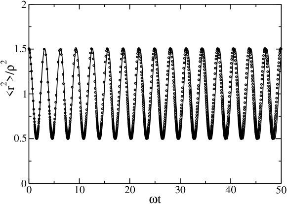
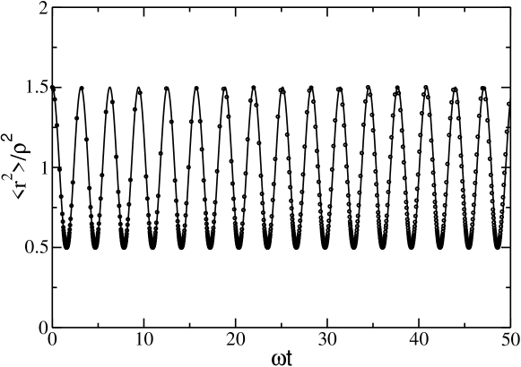
In Fig. 1, is plotted as a function of the dimensionless time, , for and . The circles are the simulation results and the solid line the theoretical prediction given by Eq. (15). For the chosen values of the parameters, the density at the origin (the maximum density) oscillates between and , so that the system is supposed to be accurately described by the Boltzmann equation. The measurements of are taken each collisions per particle. That is why it is seen in the figure that the density of circles is higher when is close to the minimum. At those times the temperature and the density are close to the respective maxima and there are more collisions per particle in a given time window. As it is seen, in the time scale of the figure, the agreement between the simulation results and the theoretical prediction is very good from the initial time (as expected), oscillating with frequency around unity. This is so because, as it was discussed in Sec. III, Eq. (15) holds for any initial condition at any time. Nevertheless, a slight discrepancy between the frequency seen in the simulations and the theoretical one, , is observed. The measured time average of is around . It is not plotted because it cannot be distinguished from the theoretical prediction (unity) in the scale of the figure. Fig. 2 shows the same data as Fig. 1, but for another value of the density, . The initial scaled variance is the same that in the previous case so that . The circles are the simulation results and the solid line the theoretical prediction given by Eq. (15). As the energy is larger than in the previous case, the density is smaller and the Boltzmann prediction is expected to be even better. In fact, in this case, the discrepancy between the frequency of the simulation results and the theoretical prediction, , cannot be observed in the scale of the figure. As the measurements of are also taken each collisions per particle, the density of points depends on time in a similar way as in Fig. 1. Let us note that, for the chosen values of the parameters, the amplitude of the oscillations is of the order of the mean value () and the dynamics are highly non-linear. As discussed in Sec. III.1, the state of the system is described by an exact solution of the complete non-linear Boltzmann equation.
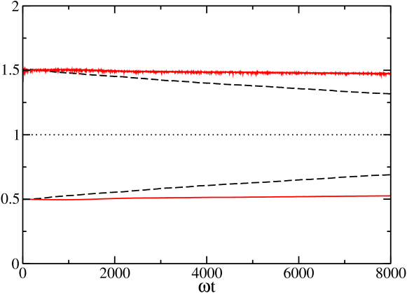
In Fig. 3, the amplitude of the oscillations of is plotted, but over a much wider time scale. The solid line (red) corresponds to , while the dashed line (black) is for . The point line is at unity and is plotted only for reference. It is seen that the amplitudes decay very slowly, with faster decay for the one associated to the larger density. These effects (decay of the amplitude and corrections to the frequency and time average value) are beyond Boltzmann and will be discussed in the following sections. In any case, there is a wide time scale in which the Boltzmann prediction is accurate, and that we study in more detail below.
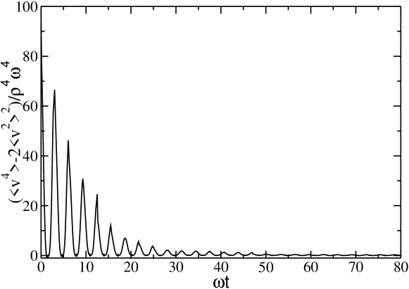
To see that the system reaches the breather state, we have measured the fourth position and velocity moments of the distribution function, and respectively. In the breather state, due to the Gaussian character of the distribution function, these moments are simply related to their respective second moments. In the case, we get
| (39) | |||
| (40) |
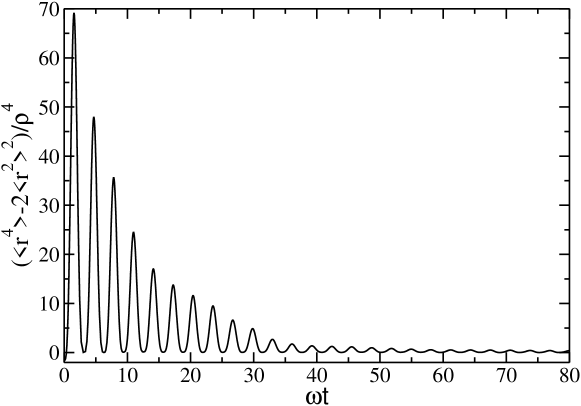
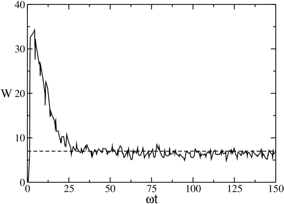
In Fig. 4, MD simulation results for are plotted as a function of the dimensionless time, , for and . It can be seen that, for times (around collisions per particle), the simulation results are close to zero, indicating that the breather state has been reached. Similarly, In Fig. 5, MD simulation results for are plotted as a function of time, for the same values of the parameters. Again, for times , the simulation results are close to zero, indicating that the breather state has been reached. It is also possible to determine if the system has reached the breather state by measuring the total number of particles inside a “small” sphere in the position and velocity space centered at the origin. By small, it is understood that the distribution function does not vary appreciably inside it. This is so because the distribution function of the breather at the origin is simply , that is time-independent (a similar quantity was considered in Dauchet et al. (2018) to measure the damping of the breathing mode). In Fig. 6, the total number of particles inside a sphere centered at the origin in the position and velocity space of radius and respectively, , is plotted as a function of the dimensionless time, , for and . As the phase-space volume is “small”, it is
| (41) |
with and . The solid line are the simulation results and the dashed line the theoretical prediction in the breather state. Although the quantity fluctuates much more than and , it can safely be said that, for (see Fig. 6), the breather value has been reached. Note that, unlike the fourth moments, and , does not oscillate in the transient to the breather state. The results for and are similar, finding that, after around collisions per particle (in this case ) , and reach the corresponding values in the breather state.
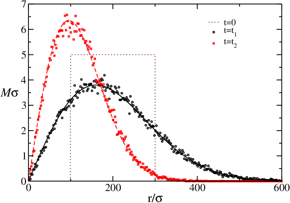
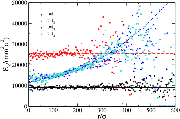
With the aid of the above defined quantities, it is possible to determine if the breather state has been reached. In particular, the measured values of the fourth position and velocity moments indicate that the distribution function is Gaussian. The objective now is to measure the hydrodynamic fields once the breather state has been reached, in order to compare them with the theoretical predictions. Concretely, the spatial domain of the system has been divided into rings of internal radius and external radius , that will be denoted as , and three quantities (functions of ) have been measured at different times: (a) the number of particles in the ring, ; (b) the averaged radial component of the velocity in the ring, and; (c) the averaged kinetic energy in the ring, . The subindex indicates that the sum is extended over the particles that are inside the ring . From Eqs. (29) and (30), the theoretical expressions for the above defined quantities can be calculated in the breather. Assuming that is small enough and for , they are: , and . We have taken , which satisfies the desired condition that the hydrodynamic fields do not vary appreciably over distances of this order.
The following MD simulation results are also for and . In Fig. 7, is plotted for the initial time, for (where is approximately maximum) and for which is the value of the available dimensionless time closest to (where is approximately minimum). As mention above, for these values of the parameters, the system is well in the breather state for these times. The dots, (black) circles and (red) squares are the simulation results for the initial condition, and respectively. The (black) solid and the (red) dashed lines are the theoretical predictions for and respectively. With the chosen parameters, the values of and are and respectively, so that is only different from zero for where it is constant. It is seen that the agreement between the simulation results and the theoretical prediction is remarkable. For with and being not too large for the amplitude of to have decayed, a very similar profile to the one measured at time is obtained. The same occurs for the profiles at and the one measured at time .
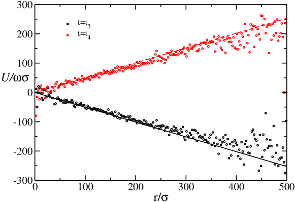
In Fig. 8, is plotted for the available times closer to and that will be denoted as and respectively. For these times the absolute value of the slope of the velocity profile is approximately maximum. The (black) circles and (red) squares are the simulation results at time and respectively and the (black) solid and (red) dashed lines are the corresponding theoretical prediction. It is seen that the agreement between the simulation results and the theoretical prediction is very good from the origin to . For the data becomes more noisy because there are very few particles (at those times, the number of particles that are inside the circle centered at the origin of radius is about so that the number of particles outside the circle is about ). In fact, as it can be seen in the figure, there are several cells where there are no particles. at times and is not shown, but it fluctuates around zero.
In Fig. 9, is plotted for , , and . The (black) circles, (red) squares, (dark blue) triangles and (sky blue) stars are the simulation results for , , and respectively, and the (black) solid, (red) dashed and (dark blue) solid-dashed lines the corresponding theoretical prediction. The agreement between the simulation results and the theoretical prediction is very good from the origin to , and for the times , and (the same for ) respectively. As in the previous case of , above these values of the distance to the origin, the data become very noisy.
All these results indicate that for times of the order of the system is already in the breather state where it remains for long time. Similar results are obtained starting with different initial conditions and for different values of the parameters if the density is small enough, proving the attractive character of the breather state at the Boltzmann level.
IV Breathers beyond the Boltzmann equation description
The objective of this section is the study of the existence of the breather states beyond the low density limit. The question we want to address is: for the considered model at finite densities, is a breather state or, on the contrary, equilibrium reached in the long-time limit?
We have shown in Sec. III that one of the essential features not to reach equilibrium in the low density limit is the fact that we have a closed equation for , Eq. (14). The solution of this equation is given by Eq. (15), where it is manifestly seen that equilibrium can only be reached for a particular class of initial conditions. It was also shown in Sec. III by intuitive arguments that, to have the above mentioned closed description, it is essential that the particles be point-like. Hence, we expect not to have a closed description for in a finite density system. On the other hand, for a finite density system of hard spheres, the so-called Enskog equation is supposed to describe the dynamics of the system if the density is “moderate” Enskog (1922); van Beijeren and Ernst (1973); Résibois and Leener (1977). The structure of the Enskog equation is similar to that of the Boltzmann equation, but with the collisional term modified in such a way that the size of the particles as well as the existence of spatial correlations between the colliding particles are considered. For this equation, a -theorem has been proved Résibois (1978); Maynar et al. (2018) but, in this case, the condition for the long-time behavior of is
| (42) |
where, in contrast to Eq. (37), and depend only on time but not on the position. The new function, , is included here because total angular momentum is conserved in a collision (in the Boltzmann framework this term is included in the that can depend on ). The difference between Eq. (37) and (42) is due to the fact that, at the Enskog level, is not approximated by (as it is done at the Boltzmann level in which the size of the particles is neglected). Then, in a collision, it is taken into account that particles are located at different places. For example, , while due to conservation of total momentum in a collision (the same occurs with and ). The fact that, at the Enskog level, can only depend on time forbids the existence of the breather and equilibrium is always reached.
For the above mentioned reasons, it is expected that the system will always reach equilibrium in the long-time limit. Nevertheless, we would also expect that, if the system is dilute enough, the Boltzmann description will provide a good approximation of the dynamics and the system will reach a state close to the breather where it will remain for some time. In order to study this situation, we will start by a Liouville description of the system. The first equation of the BBGKY hierarchy is Cercignani (1988)
| (43) |
where
| (44) |
being the two-particle distribution function of the colliding particles. Note that the Boltzmann equation is obtained by making the approximation , i.e. neglecting position and velocity correlations and the variation of the one-particle distribution function in distances of the order of the diameter of the particles.
Performing a similar analysis to the one made in the previous section with the Boltzmann equation, i.e. by taking moments in Eq. (43), one obtains (see Appendix A)
| (45) | |||||
| (46) |
where is the collisional contribution to the pressure tensor. Its explicit expression is
| (47) |
where
| (48) |
Physically, represents the contribution to the flux of momentum due to collisions Maynar et al. (2018). In a hard sphere system, there is flux of momentum through a given surface due to particles that cross the surface, , and due to collisions between particles without crossing the surface (the two particles are in opposite sites of the surface, do not cross the surface, but interchange momentum in a collision). The first contribution is described simply by the tensor , while the second, , is given by Eq. (47).
Eqs. (45) and (46) are exact but, in contrast to the Boltzmann ones given by (11) and (12), they are not closed. They depend on that is unknown. Moreover, this new term is a collisional contribution which arises from the fact that, in a collision, particles are not at the same place due to their finite size (see Eq. (47)). So, everything is consistent with the intuitive explanation of Eq. (14) in which it was essential that the particles were “at the same place” in a collision in order to have a closed equation for : for finite size particles the evolution equation for is not closed due to a collisional contribution that vanishes for point particles. In fact, an intuitive derivation of Eqs. (45) and (46) can be made in the same lines as in the Boltzmann context. In effect, in this case changes instantaneously in a collision. Concretely, , where has been defined taking the particle as the tagged particle. Note that the increment is always positive because when a collision is going to take place. Hence, the change of in a time window due to collisions is the sum of for all the collisions taking place in . The average of this quantity is precisely the new contribution .
In order to study Eqs. (45) and (46) some approximations have to be done. Firstly, we will assume molecular chaos, i.e.
| (49) |
without the approximation . This is the simplest approximation that still takes into account the fact that, in a collision, particles are not at the same place. To continue, we need to express the distribution function as functionals of and . The simulation results of the previous section show that, for the considered values of the parameters, the one particle distribution function of the finite density system is very well characterized by the distribution function of the breather at the Boltzmann level. This is so on the time scale in which the amplitude of the breather does not vary. For this reason, we assume that the distribution function has the same functional form in terms of and as the distribution function of the breather at the Boltzmann level. Taking into account Eqs. (28), (29) and (30), the distribution is then approximated by
| (50) |
with
| (51) | |||||
| (52) |
The inverse of the temperature, , is given in terms of and by Eq. (36)
| (53) |
As the distribution function of the breather is an exact solution of the Boltzmann equation in all the regimes, i.e. from the collisionless to the hydrodynamic regime, our approximation is expected to be valid in all the regimes aswell.
Taking into account molecular chaos and inserting Eq. (50) into Eq. (47), the expression for to first order in the gradients is (see Appendix B)
| (54) |
where the zeroth and first order terms are
| (55) |
and
| (56) |
respectively. Note that is proportional to consistently with the fact that we are beyond the Boltzmann framework.
Let us remark that the same result is obtained in a simpler way (without any calculation) if, for , we take the hydrodynamics expression at the Enskog level to first order in the gradients and neglect position correlation Ferziger and Kaper (1972); Garzó et al. (2018) (taking the pair correlation function equal to unity) as it was done in García de Soria et al. (2024). In effect, the hydrodynamic expression for to first order in the gradients is Résibois and Leener (1977)
| (57) |
where is the excess pressure with respect to the ideal one, , is the collisional contribution to the shear viscosity, is the bulk viscosity and denotes the -th component of . The explicit expression for and are (the coefficient is not needed in the subsequent analysis)
| (58) |
and
| (59) |
where is the pair correlation function at contact. The trace of the tensor is
| (60) |
Taking into account the explicit expressions for and given above and approximating the two-pair correlation function by unity, Eq. (60) reduces to Eq. (54) with the zeroth order and first order in the gradients contribution given by Eqs. (55) and (56) respectively. The coincidence between the kinetic theory approach and the hydrodynamic approach deserves some comments as it is not incidental: in the kinetic theory approach the distribution function is Gaussian, while in the hydrodynamic one the distribution function to first order in the gradients is not Gaussian. Nevertheless, the non gaussianities contribution to are all immersed in the shear viscosity, that does not appear in the trace. Let us also remark that, in the hydrodynamic approach, it is implicitly assumed that the fields vary over distances much larger than the mean free path while, in the kinetic approach, it is only assumed that the fields vary smoothly over distances of the order of the diameter of the particles (so that the expansion given by Eq. (54) makes sense).
Finally, taking into account the expressions for the hydrodynamic fields, Eqs. (51), (52) and (53), the spatial integral of the pressure tensor can be evaluated, obtaining
| (61) | |||||
| (62) |
where the value of the maximum density (the one at the origin) at the Boltzmann level at time has been introduced
| (63) |
Eqs. (45) and (46) with given by Eqs. (61) and (62) form a closed set of first order non-linear differential equations for and . They are valid arbitrary far from equilibrium if the hypothesis we have postulated are valid, i.e. if Eqs. (49), (50) and (54) hold. In the next section, we will analyze the equation for states close to equilibrium.
IV.1 Close to equilibrium states
In this section, the dynamics of the system are studied for states close to thermal equilibrium. It is convenient to work with the second order differential equation for equivalent to the system of Eqs. (45) and (46) that reads
| (64) |
where is given by Eqs. (61) and (62) with . Eq. (64) admits a stationary solution (the equilibrium solution), , that satisfies
| (65) |
with . differs from the corresponding Boltzmann value, , due to excluded volume effects. Assuming that the density is small, should be close to . It is convenient to introduce the deviation
| (66) |
that, to linear order, can be calculated, obtaining
| (67) |
where is the value of the maximum density of a system in equilibrium with energy per particle, , at the Boltzmann level, defined in Eq. (38). Of course, . Remarkably, the prediction for given by Eq. (67) coincides with the equilibrium one in the first virial approximation (see Appendix C).
To study the dynamics, we introduce the deviation of around the actual equilibrium value
| (68) |
To linear order in and for low densities, we have
| (69) | |||||
| (70) |
Taking into account the above relations, by linearizing Eq. (64) around the equilibrium solution, one finds that, for low densities, satisfies the following second order linear differential equation with constant coefficients
| (71) |
with
| (72) |
and
| (73) |
The solution of the differential equation can be written in terms of the roots of the characteristic equation, ,
| (74) |
where, again, the linear approximation in has been made. Then, within this approximation, the solution of Eq. (71) can be written as
| (75) |
with the phase, , depending on the initial condition. The coefficient , given by Eq. (72), is identified as the relaxation time of the amplitude of the oscillations, and , given by Eq.(73), is the frequency of the oscillations. This is the main result of the paper as it lets us understand the origin of the relaxation to equilibrium as a consequence of density corrections with respect to the Boltzmann framework. The relaxation time, , depends on the two parameters that define the equilibrium state, and (or, equivalently, and ). In the conditions we are working (for low densities), the relaxation is very slow, as the relaxation time goes as . The divergence in the low density limit is consistent with the Boltzmann description, in which equilibrium is never reached. On the other hand, the frequency of the oscillations, , is “renormalized” with respect to the Boltzmann prediction, , being the former one always larger than the last one. The origin of the renormalization of the frequency and of the damping can be identified: from Eq. (69), it is seen that the renormalization of the frequency (and also of the time average of the oscillations) comes from while, from Eq. (70), it is seen that the damping comes from . These results are equivalent to the ones obtained in García de Soria et al. (2024) by hydrodynamic arguments where is associated to the excess pressure and to the bulk viscosity. Concretely, in García de Soria et al. (2024) the relaxation time, , was identified as a functional of the bulk viscosity in equilibrium, , in the form
| (76) |
that coincides with Eq. (72). Eq. (75) highlights the two time scales of the state of the system: the one related to the oscillations, , that is fast and it is given by the external force, and that controls the decay of the amplitude of the oscillations and that is much slower than the previous one.
IV.2 Simulation results
The objective of this section is to compare the theoretical predictions obtained above with MD simulation results. The idea is to measure as a function of time, extracting from it , and . is obtained from the averaged value around which oscillates, by fitting the relative maxima (or minima) to an exponential and by measuring the time between two relative maxima (or minima) that can be separated by several periods. The MD simulations are performed as in section III.2. The only difference is that the initial condition is generated in such a way that the initial density profile is Gaussian. Hence, at the initial time the system is closer to the breather and the condition for the theory to be valid, i.e. that the distribution function has the same functional form that the breather at the Boltzmann level, is reached faster.
We have performed a series of simulations with disks and for different values of the energy, in such a way that varies approximately in the interval . These values of the density are expected to be small enough for the theory to be valid, as the Boltzmann prediction describes accurately the dynamics in a wide enough time window. The results have been averaged over trajectories. With the chosen values of the parameters, the system is close enough to equilibrium so that the linear approximation is supposed to be valid. This is supported by the fact that the non-linear solution of Eqs. (45) and (46) with given by Eqs. (61) and (62) is very close to the linear approximation for the above mentioned parameters. For the considered values of the parameters, the minimum mean free path (the one at the origin) is of the same order as the size of the system measured by , so that the conditions for the validity of hydrodynamics are doubtful. Nevertheless, this is not relevant in our case because, as it has been mentioned above, our predictions do not rely on a hydrodynamic description. In addition, this gives support to the analysis performed in García de Soria et al. (2024), as the theoretical predictions do not depend on the regime.
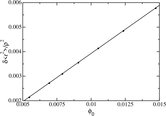
.
In Fig. 10, is plotted as a function of the dimensionless density, . The dots are the simulation results and the solid line the theoretical prediction given by Eq. (67). As can be seen, the agreement between them is excellent.
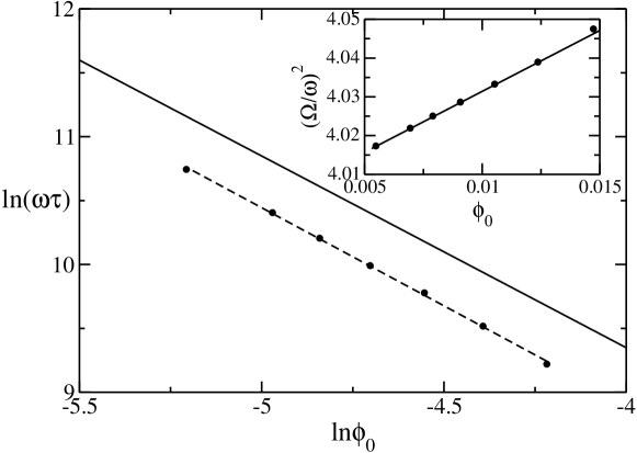
In Fig. 11, is plotted as a function of in logarithmic scale. The dots are the simulation results and the solid line the theoretical prediction given by Eq. (72) that, for and expressed in terms of and , takes the form
| (77) |
The dashed line is the linear fitting of the simulation results with slope in good agreement with Eq. (77). As in the previous cases, the error bars cannot be observed in the scale of the figure. Note that, in this case, the agreement is not as good as in the previous two quantities. The quotient between the theoretical prediction and the measured quantities is always of the order of , indicating that, although the density dependence is perfectly captured by the theory, there are other not considered ingredients that renormalize the amplitude of . Similar results are obtained for other values of the number of particles, so that the discrepancies are not due to finite size effects. In the next section we will further comment about that.
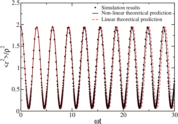
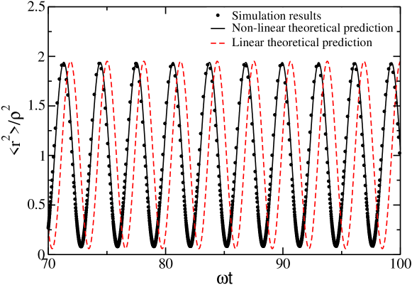
Finally, is plotted as a function of the dimensionless density, , in the inset of Fig. 11. The dots are the simulation results and the solid line the theoretical prediction given by Eq. (73).The agreement between the simulation results and the theoretical prediction is very good. The error bars in the measured quantities cannot be observed in the scale of the figures. We have also performed MD simulations very far from equilibrium where the linear approximation is supposed to fail. The values of the chosen parameters are , and the “extreme” value , so that the amplitude of the oscillations of is nearly . In Fig. 12, is plotted as a function of the dimensionless time, , in the time window . The points are MD simulation results, the (black) solid line is the non-linear theoretical prediction, while the (red) dashed line is the linear theoretical prediction. It can be seen that the agreement between the simulation results and the theoretical predictions is very good, although a small shift is found in the linear theoretical prediction for . This effect is amplified in Fig. 13, where the same is plotted but for the time window . Here, the linear theoretical prediction is clearly shifted with respect to the simulation results, while the non-linear one still perfectly fits the simulation data. More quantitatively, the values of the frequencies of the oscillations, , in the simulation results, non-linear theoretical prediction and linear theoretical predictions are , and respectively. We stress that the “correction” to the Boltzmann prediction in the non-linear case is of the order of twice the correction in the linear case. Note also that, for these times, the decay of the amplitude of the oscillations cannot be observed. The same analysis has been performed for different values of the relative amplitude, , the results being plotted in Fig. 14. The (black) circles are the simulation results and the (red) squares are the results extracted from the numerical solution of the non-linear equations. It is seen that the agreement between both is very good and that for the linear prediction is accurate. These results give a strong support to the validity of the non-linear equations, at least in the time window where dominates the dynamics with respect .

V Discussion and conclusions
In this work, we have worked out the dynamics of a system of hard particles that collide elastically and that are confined by an isotropic harmonic potential: each particle of mass at point is subject to a force . The study has been performed at two levels of description: at the low-density limit where the Boltzmann equation describes the dynamics of the system and beyond the low-density limit (although for low densities). At the Boltzmann level, we have shown that, independently of the initial condition, the system reaches a breather state in the long-time limit. Concretely, if the system is studied in the frame of reference where total momentum vanishes and assuming the total angular momentum also vanishes, the breather is characterized by (number of particles), , where refers to an average in the initial condition, and the total energy per particle . This is a consequence of the fact that verifies a closed equation, independently of the initial distribution function, oscillating around the equilibrium value with frequency (the amplitude of the oscillations depends on and ). Equilibrium is only reached when and vanishes. For low densities, MD simulation results are in excellent agreement with the Boltzmann predictions. We have probed the above mentioned prediction for and we have shown that, independently of the initial condition, after some collisions per particle, the hydrodynamic fields reach the corresponding profiles, oscillating with the corresponding frequency. Nevertheless, small corrections are reported, eroding the amplitude of the oscillations very slowly. The frequency of the oscillations and the mean value of are also slightly renormalized. All these effects are due to the fact that a system of particles of finite diameter, , does never, strictly speaking, comply with the Boltzmann equation level of description.
The study of the dynamics of the system beyond the Boltzmann equation is performed taking into account precisely this idea. By performing the approximation in the first equation of the BBGKY hierarchy, a closed equation for the distribution function is obtained that takes into account the finite size of the particles. Recall that the Boltzmann equation is obtained with the additional approximation . By taking moments in the dynamical equation, evolution equations for and are obtained that, in contrast to the Boltzmann ones, are not closed. A new term arises that is proportional to the total collisional contribution to the pressure, . Closed evolution equations are obtained by assuming that the functional dependence of the distribution function on and is the same as the one in the breather state at the Boltzmann level (this approximation is supported by the previous MD simulation results) and by expanding the distribution function to first order in the gradients. By performing a linear analysis of the resulting equations, one finds that oscillates around the equilibrium value (that is renormalized with respect to the Boltzmann value) with a given frequency (that is also renormalized with respect to the Boltzmann prediction), leading to a decay of the amplitude of the oscillations with a given relaxation time, . While the renormalizations are due to the zeroth order in the gradients expansion of , i.e. the excess pressure, the decay of the oscillations is due to the first order contribution. If a hydrodynamic description of the system is valid, this first order contribution can be understood as a fingerprint of the bulk viscosity García de Soria et al. (2024). In fact, the measure of can be considered to be a direct probe of the bulk viscosity. We are not aware of any other process in which this transport coefficient appears in such a clear way.
The agreement between the theoretical predictions and Molecular Dynamics simulation results is excellent for the mean value and frequency of the oscillations. For , the agreement is decent, but it is not as good as for the aforementioned quantities. This fact deserves some comments. First, it must be mentioned that the mismatch is not caused by the linearization process, as the numerical solution of the complete non-linear equations leads to similar results. To analyze the problem, recall the main approximations made in the theory: a) Eq. (49), i.e. molecular chaos assumption ; b) Eq. (50), that approximates the distribution function to have the same functional form as in the breather state at the Boltzmann level with the hydrodynamic fields written in terms of and ; c) the expansion in the gradients of the fields. Considering a), position correlations between the particles that are going to collide can be accounted for by multiplying the collisional term by the pair correlation function at contact. This is the idea behind the Enskog equation Enskog (1922) that incorporates position correlations of the particles at contact while neglecting velocity correlations. This would actually increase the collision frequency and, hence, “accelerate” the process, obtaining a faster decay, as desired. However, for the considered densities, the corrections cannot reach the factor as the pair correlation function at contact is of the order of , hence a 2% correction. Although the density is very small, velocity correlations could contribute to the corresponding order in the density. However, their computation are complex and the analysis would require further investigations. Approximation c) could be improved by introducing more terms in the gradients expansion but it can hardly explain the discrepancy: as is a scalar, the second order in the gradients contribution is of the form , where with are Burnett coefficients, that do not contribute to in the linear regime (in the non-linear case, a term of the form will appear that would not help, either). Perhaps, the most plausible scenario to explain the discrepancies is that approximation b) is not accurate enough at this order in the density. Within a hydrodynamic description, this could be improved by considering the hydrodynamic equations at the Enskog level. By linearizing them around the equilibrium state, the relaxation time could be extracted, although it is difficult to go beyond the approximation performed in García de Soria et al. (2024) as the state around which the linearization is performed is position-dependent. Another possibility is to modify the ansatz given by Eq. (50) by incorporating more moments in the distribution function, e.g. all the possible position and velocity fourth moments. Taking into account the symmetry of the system, they are , , , , and . Work along these lines is in progress.
The present work represents a first step in the study of the dynamics of dense confined systems. A number of interesting questions arise, pertaining to the behavior at high densities, or under anisotropic trapping. In the latter case, the decay to equilibrium features two contributions, one coming from the anisotropy of the potential and one stemming from the finite density. It would be interesting to clarify the region of the parameters where one effect or the other dominates. Work along these lines is also in progress.
Acknowledgements.
This research was supported by grant ProyExcel-00505 funded by Junta de Andalucía, and grant PID2021-126348NB-100 funded by MCIN/AEI/10.13039/501100011033 and ERDF “A way of making Europe” and by the ‘Agence Nationale de la Recherche’ grant No. ANR-18-CE30-0013.Appendix A Evolution equations for and
We will proceed in two steps. We will first take velocity moments in Eq. (43) to obtain balance equations for and and, then, we will take spatial moments to obtain the desired equations.
By integrating in the velocity in Eq. (43) and taking into account that Maynar et al. (2018), the density equation is obtained
| (78) |
By multiplying by in Eq. (43) and integrating in the velocity space, one obtains
| (79) |
where the collisional contribution to the pressure tensor has been introduced through
| (80) |
with
| (81) |
and we have taken into account (see Ref. Maynar et al. (2018)) that
| (82) |
Appendix B Gradient expansion of
Taking into account molecular chaos, i.e. Eq. (49), into Eq. (47), the expression for is
| (84) |
where we have also replaced by . By expanding the integrand to first order in the gradients, it is
| (85) |
And, by substituting Eq. (85) into (84), we have
| (86) |
with
| (87) | |||
| (88) |
where the integral in has been performed.
Taking into account that the distribution function has the form given by Eq. (50), the zeroth order contribution is
where the new variables, and , have been introduced. The notation is also used. Finally, taking into account that
| (90) |
and performing the Gaussian velocity integrals, one obtains
| (91) |
Taking into account that
| (92) |
the first order contribution is
| (93) |
In addition, the gradient of the distribution function can be explicitly written in the form
| (94) |
where the summation over repeated indexes has been used. By substituting Eq. (B) into Eq. (93), taking into account symmetry properties and performing the Gaussian velocity integrals, the expression for of the main text is obtained, i.e.
| (95) |
Appendix C Evaluation of in the first virial approximation
The objective of this appendix is to calculate in the first virial approximation. Let us assume that the state of the system is described, in equilibrium, by the canonical -particle density
| (96) |
where the notation has been introduced and
| (97) |
where . In equilibrium, we have
| (98) |
where .
Let us first evaluate the denominator of Eq. (98). It can be rewritten in the form
| (99) |
The second term can be calculated
| (100) |
In order to evaluate the first term, it is assumed that the main contribution comes from the volume in for which only two particles overlap
| (101) |
Assuming that the exponential does not vary appreciably in distances of the order of , by standard manipulations, we have
| (102) |
and, by substituting it into Eq. (101)
| (103) |
Finally, taking into account Eqs. (100) and (103), Eq. (99) reads
| (104) |
To calculate the numerator of Eq. (98), we proceed in a similar fashion.
| (105) |
The second term reads
| (106) |
As above, in order to evaluate the first term, it is assumed that the main contribution comes from the volume in for which only two particles overlap
| (107) | |||
| (108) |
Again, assuming that the exponential does not vary appreciably in distances of order ,
| (109) |
Taking into account Eqs. (102), (109) and performing the Gaussian integrals
| (110) |
and, then, with the aid of Eqs. (106) and (110), Eq. (105) reads
| (111) |
By substituting Eqs. (104) and (111) into Eq. (98), one obtains
| (112) |
where used have been done of the definition of . Let us remark that, here, is the actual temperature. In order to obtain the expression of the main text, it is necessary to express as a function of . Using and the relation between the actual temperature and kinetic energy, i.e. , one obtains (assuming that is close to )
| (113) |
where . By substituting Eq. (113) into Eq. (112), one finally obtains
| (114) |
that coincides with the expression of the main text, Eq. (67).
References
- Boltzmann (1995) L. Boltzmann, Lectures on Gas Theory (Dover, New York, 1995).
- Résibois and Leener (1977) P. Résibois and M. D. Leener, Classical Kinetic Theory of Fluids (Wiley and Sons, New York, 1977).
- Cercignani (1988) C. Cercignani, The Boltzmann Equation and Its Applications (Springer Verlag, New York, 1988).
- Landford III (1975) O. E. Landford III, in Proc. 1974 Batelle Rencontre on Dynamical Systems, edited by J. Moser (Springer, Berlin, 1975) pp. 1–111.
- Landford III (1983) O. E. Landford III, in Nonequilibrium Phenomena I The Boltzmann Equation, edited by J. L. Lebowitz and E. W. Montroll (North-Holland, Amsterdam, 1983).
- (6) Strictly speaking the Boltzmann equation is obtained in the so-called Grad limit. For spheres of diameter the Grad limit is the double limit , with finite. This limit implies , which means that the total volume actually occupied by the particles goes to zero.
- Villani (2002) C. Villani, in Handbook of Mathematical Fluid Dynamics, edited by S. Friedlander and D. Serre (Elsevier Science, New York, 2002).
- Saint-Raymond (2009) L. Saint-Raymond, Hydrodynamic Limits of the Boltzmann Equation (Lecture Notes in Mathematics (Springer), Berlin, 2009).
- Succi (2018) S. Succi, The lattice Boltzmann equation for complex states of flowing matter (Oxford University Press, Oxford, 2018).
- Boltzmann (1909) L. Boltzmann, in Wissenschaftliche Abhandlungen, edited by F. Hasenorl (J. A. Barth, Leipzig Vol II, 1909).
- Guéry-Odelin et al. (2014) D. Guéry-Odelin, J. G. Muga, M. J. Ruiz-Montero, and E. Trizac, Phys. Rev. Lett. 112, 180602 (2014).
- Guéry-Odelin et al. (2023) D. Guéry-Odelin, C. Jarzynski, C. A. Plata, A. Prados, and E. Trizac, Reports on Progress in Physics 86, 035902 (2023).
- Uhlenbeck (1963) G. E. Uhlenbeck, Lectures in Statistical Mechanics (American Mathematical Society, Providence, 1963).
- Dalfovo et al. (1999) F. Dalfovo, S. Giorgini, L. P. Pitaevskii, and S. Stringari, Rev. Mod. Phys. 71, 463 (1999).
- Guéry-Odelin et al. (1999) D. Guéry-Odelin, F. Zambelli, J. Dalibard, and S. Stringari, Phys. Rev. A 60, 4851 (1999).
- Buggle et al. (2005) C. Buggle, P. Pedri, W. von Klitzing, and J. T. M. Walraven, Phys. Rev. A 72, 043610 (2005).
- Lobster et al. (2015) D. S. Lobster, A. E. S. Barentine, E. A. Cornell, and H. J. Lewandowski, Nat. Phys. 11, 1009 (2015).
- Guéry-Odelin and Trizac (2015) D. Guéry-Odelin and E. Trizac, Nat. Phys. 11, 988 (2015).
- García de Soria et al. (2024) M. I. García de Soria, P. Maynar, D. Guéry-Odelin, and E. Trizac, Phys. Rev. Lett. 132, 027101 (2024).
- Allen and Tisdesley (1987) M. P. Allen and D. J. Tisdesley, Computer Simulations of Liquids (Oxford Science Publications, New York, 1987).
- Dauchet et al. (2018) J. Dauchet, J.-J. Bezian, S. Blanco, and et al, Sci. Rep. 8, 13302 (2018).
- Enskog (1922) D. Enskog, Kungl. Sv. Vetenskapsakad. Hand 63, 3 (1922).
- van Beijeren and Ernst (1973) H. van Beijeren and M. H. Ernst, Physica 68, 437 (1973).
- Résibois (1978) P. Résibois, Phys. Rev. Lett. 40 (1978).
- Maynar et al. (2018) P. Maynar, M. I. García de Soria, and J. J. Brey, J. Stat. Phys 170, 999 (2018).
- Ferziger and Kaper (1972) J. Ferziger and H. Kaper, Mathematical Theory of Transport Processes in Gases (North-Holland, Amsterdam, 1972).
- Garzó et al. (2018) V. Garzó, R. Brito, and R. Soto, Phys. Rev. E 98 (2018).