Selling Joint Ads: A Regret Minimization Perspective

Abstract

Motivated by online retail, we consider the problem of selling one item (e.g., an ad slot) to two non-excludable buyers (say, a merchant and a brand). This problem captures, for example, situations where a merchant and a brand cooperatively bid in an auction to advertise a product, and both benefit from the ad being shown. A mechanism collects bids from the two and decides whether to allocate and which payments the two parties should make. This gives rise to intricate incentive compatibility constraints, e.g., on how to split payments between the two parties. We approach the problem of finding a revenue-maximizing incentive-compatible mechanism from an online learning perspective; this poses significant technical challenges. First, the action space (the class of all possible mechanisms) is huge; second, the function that maps mechanisms to revenue is highly irregular, ruling out standard discretization-based approaches.

In the stochastic setting, where agents’ valuations are drawn according to some fixed but unknown distribution, we design an efficient learning algorithm achieving a regret bound of $O(T^{\nicefrac{{3}}{{4}}})$. Our approach is based on an adaptive discretization scheme of the space of mechanisms, as any non-adaptive discretization fails to achieve sublinear regret. In the adversarial setting, when the valuations are arbitrarily generated upfront, we exploit the non-Lipschitzness of the problem to prove a strong negative result, namely that no learning algorithm can achieve more than half of the revenue of the best fixed mechanism in hindsight. We then consider the $\sigma$-smooth adversary, which randomly generates the valuations from smooth distributions but, unlike in the stochastic case, can do so in a non-stationary way. In this setting, we construct an efficient learning algorithm that achieves a regret bound of $O(T^{\nicefrac{{2}}{{3}}})$ and builds on a succinct encoding of exponentially many experts. Finally, we prove that no learning algorithm can achieve less than $\Omega(\sqrt{T})$ regret, in both the stochastic and the smooth setting, thus narrowing the range where the minimax regret rates for these two problems lie.

1 Introduction

Consider an online retail website such as Amazon or Alibaba. These websites sell goods directly but also serve as middlemen between buyers and sellers. Moreover, they typically feature ads by which a certain offer can appear more prominently on a search results page. A crucial feature of these ads is that they may simultaneously benefit a brand and a merchant (say Nike and Footlocker). This is precisely what happens in Facebook’s “Collaborative Ads” program (Facebook, 2024), where brands and merchants cooperate to purchase joint ads.

Situations like this, where a brand and a merchant cooperatively bid in an auction, are a prime motivation for designing selling mechanisms for a single, non-excludable good (Güth and Hellwig, 1986). The mechanism — whose goal is revenue maximization — collects bids from the merchant and the brand and decides whether it wants to allocate the good (show the ad). In the cases where it allocates, the mechanism decides on a payment and how it will be split between the two parties. We call the problem of designing such revenue-maximizing mechanism the Joint Ads Problem. Non-excludable mechanism design problems like this give rise to intricate incentive constraints: Unless we set up the mechanism in an incentive-compatible way, the merchant (or the brand) may try to shade their bid, thereby transferring part of the costs to the other party. An incentive-compatible mechanism prevents such gaming opportunities and ensures that it is in the agents’ best interest to report their valuations truthfully. While the “one-shot” task of selling a single, non-excludable, public good is well understood (Güth and Hellwig, 1986; Csapó and Müller, 2013), it requires strong informational assumptions, e.g., the agents’ valuations need to be drawn (independently) from regular or finitely supported distributions which are perfectly known. For practical purposes, a more data-driven approach is desirable.

Following Kleinberg and Leighton (2003), we approach the design of an incentive-compatible revenue-maximizing mechanism for the Joint Ads Problem from an online learning perspective. Formally, we study the Repeated Joint Ads problem, where a mechanism designer interacts at each time step $t=1,\ldots,T$, with a new pair of agents (e.g., merchant and brand) that want to purchase an item (e.g., an ad slot). Each of these two agents $i\in\{1,2\}$ is characterized by a private valuation $v_{i}^{t}$ representing its willingness to pay. The mechanism designer (that we often refer to as learner) posts a dominant-strategy-incentive-compatible (DSIC) and individually-rational (IR) mechanism $M^{t}$. The agents’ valuations and the mechanism induce a revenue $\textsf{rev}_{t}(M^{t})$ for the learner, given by the sum of the two agents’ payments. The mechanism designer’s goal is to maximize revenue, and the performance of a learning algorithm is measured in terms of its regret: the difference between the revenue achieved and that of the best fixed DSIC and IR mechanism.

The best fixed mechanism is an ambitious benchmark, which differentiates us, for instance, from the line of work on second price auctions with reserve price(s) (e.g., Cesa-Bianchi et al., 2015; Roughgarden and Wang, 2019), where the regret is measured with respect to the best fixed reserve price(s). We investigate three possible models generating the agents valuations: (i) the adversarial setting, where valuations are generated up-front in an arbitrary way; (ii) the stochastic setting, where valuations are drawn i.i.d. from a fixed but unknown distribution; and (iii) the $\sigma$-smooth setting (Haghtalab et al., 2020, 2021), where the valuations are drawn from a sequence of distributions that are not too concentrated (see Section 2 for formal definitions). Note that, in the stochastic i.i.d. case, the benchmark coincides with the best Bayesian mechanism, but unlike in the “one-shot” Bayesian mechanism, the input distribution is not known in advance and has to be learned on the fly. Settings (ii) and (iii) are both considered weaker adversaries than (i), as they consider valuations that are generated randomly, but are incomparable to each other. In (ii), valuations are drawn from a fixed distribution, which can be “spiky.” In (iii), valuations are non-stationary but smooth.

1.1 Our Results

We provide an overview of our results for the Repeated Joint Ads problem, and compare them with the closest results in the literature. While our main motivation lies in its practical importance, it is also arguably the most fundamental problem for initiating the study of non-excludable mechanism design from a no-regret learning perspective.

• In the stochastic setting, we provide an efficient learning algorithm, Augment-the-Best-Mechanism, that exhibits a regret of $\tilde{O}(T^{\nicefrac{{3}}{{4}}})$ (Theorem 4), where $\tilde{O}$ hides poly-logarithmic terms. This upper bound is complemented by an $\Omega(\sqrt{T})$ lower bound (Corollary 1).

• In the adversarial setting, we prove that no learning algorithm can achieve sublinear regret with respect to the best fixed mechanism in hindsight. We actually present a stronger result: it is impossible to even approach half of the revenue of the best mechanism (Theorem 5).

• In the $\sigma$-smooth setting, we design an efficient learning algorithm, PathLearning, which achieves an $O(T^{2/3})$ regret (Theorem 6). Furthermore, we prove that any algorithm suffers regret $\Omega(\sqrt{T})$ in such setting (Theorem 8).

Together, our results paint a sharp separation between the two settings with randomly generated input and the adversarial case. As we detail below, this divide is caused by the fact that the random nature of the valuations, which is slightly different in the two models, enables two different ways of dealing with the complexities of the model (size of the action space, and irregularity of the objective function), which proves insurmountable when the input is adversarial.

Our work can be seen as generalizing the model of Kleinberg and Leighton (2003) (also previously studied by Blum et al. (2003)) from one buyer to two buyers. The first difference between the single-buyer and multi-buyer cases is that posted pricing is optimal in the former. The natural type of feedback in the single-buyer case is thus censored feedback (i.e., whether the buyer purchased or not); while in our model, optimal mechanisms are complex, and the valuations are necessary to implement payments (see Section 2.1). A second feature differentiating our model from theirs is that in the single-buyer case, the objective function, i.e., the function that maps prices to revenue, is left-Lipschitz. These differences lead to provably different regret regimes. In particular, in the single-buyer case, in the full feedback model, their results show no separation between the stochastic and the adversarial setting (the minimax regret in both cases is $\Theta(\sqrt{T})$). Our positive result in the $\sigma$-smooth setting, as opposed to the negative one in the adversarial case, further emphasizes the relevance of the smoothness paradigm as a tool to overcome adversarial lower bounds while retaining its non-stationary behavior. This phenomenon has already been observed for, e.g., general learning problems (Haghtalab et al., 2020, 2021), bilateral trade (Cesa-Bianchi et al., 2023), and first price auctions (Cesa-Bianchi et al., 2023). Closely related, Durvasula et al. (2023) investigate smoothness in revenue-maximizing auctions. However, our results are not subsumed by theirs as their work considers the incomparable setting where, at most one of $n$ buyers gets the item.

1.2 Challenges and Techniques

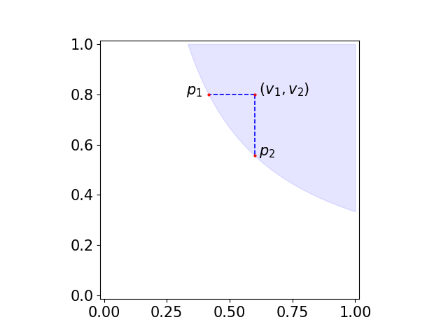
(a) Concave allocation region

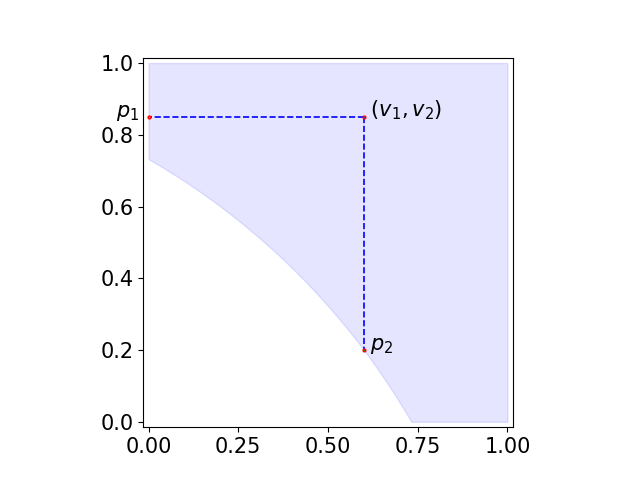
(b) Convex allocation region

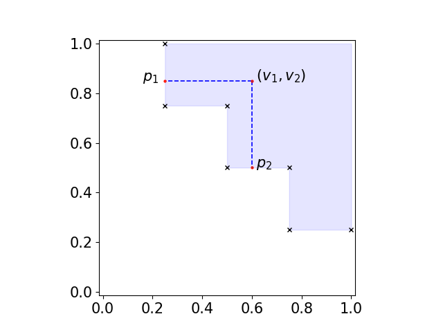
(c) Complex allocation region

Figure 1: The allocation regions of optimal mechanisms corresponding to different distributions. The payment functions can be visualized as the valuations projection on the allocation region’s boundary. For instance, in Figure 1(b), the first agent (x-axis) pays $p_{1}=0$, while the second agent (y-axis) pays $p_{2}=0.2$. The valuations are drawn i.i.d. from the distribution with cumulative density function $F(x)=2(x+1)^{-2}$ in Figure 1(a) and $F(x)=x^{2}$ in Figure 1(b). In Figure 1(c), the distribution has support on the black points.

The main technical challenge in the Repeated Joint Ads Problem is the action space: the set $\mathcal{M}$ of all DSIC and IR mechanisms is not only huge but also complex. Furthermore, the function mapping mechanisms to revenue become highly non-regular when the valuation distribution has point masses. A mechanism is characterized by two functions- an allocation and a payment rule- mapping bids to allocation and payments. Standard mechanism design arguments (Myerson, 1981) enable a simple geometric interpretation of DSIC and IR mechanisms for our problem. The allocation rule of any mechanism corresponds to a subdivision of the unit square $[0,1]^{2}$ into two regions: one in which the good is allocated and one where it’s not. For DSIC and IR, the two regions must be “north-east” monotone so that increasing either valuation can only lead to a better allocation. The payments are then given by the “south-west” projection of the valuation pair on the boundary of the allocation region. See Figure 1 for a visualization. This simplifies the problem from learning two functions to a single curve. However, the curve defining the optimal mechanism can be complex, even in simple settings. For instance, even in the (independent) Bayesian setting, the boundary of the optimal mechanism can be convex or concave (see Figures 1(a) and 1(b)). In general, for a fixed set of (possibly adversarially given) valuations pairs, the optimal allocation boundary may be neither convex nor concave (see Figure 1(c)). This notion of complexity is further reinforced by the fact that standard notions of dimensions in learning theory, e.g., VC-dimension and pseudo-dimension, are unbounded for this class (see also Section A.1). This contrasts to what happens, e.g., in Kleinberg and Leighton (2003), where the learning goal is one single number: the best fixed price.

A Hard Instance

The standard approach to solving an online learning problem on a large action space $A$ is to find a small subset $A^{\prime}\subseteq A$ with two properties (i) it is possible to achieve sublinear regret with respect the best action in $A^{\prime}$ and (ii) the performance of the best action in $A^{\prime}$ is close to that of the best action in $A$. Typically, this is done by exploiting some regularity of the learning problem, such as convexity or Lipschitzness of the objective function (Kleinberg et al., 2019; Hazan, 2016). To provide an intuition of the difficulty posed by the Repeated Joint Ads problem, we introduce the following (hard) example based on the equal revenue distribution.

Example 1 (Equal-revenue).

For any $\delta\in(0,1)$ and integer $n$, consider the random variable $V$:

$$\mathbb{P}\left(V=(\delta(1-\tfrac{1}{2^{i}}),\tfrac{1}{2^{i}})\right)=\begin{cases}2^{1-n}&\text{ for }i=1\\ 2^{i-n-1}&\text{ for }i=2,\dots,n\end{cases}$$

The random variable is supported on the $(0,1)$-$(\delta,0)$ segment (red dashed line in Figure 2), so the optimal mechanism $M^{\star}$ is clearly the one that allocates if and only if the valuations fall either on the segment itself or its right. The expected revenue of $M^{\star}$ is the sum of the payments of the two agents, which can be computed via the Myerson payment scheme (see Section 2.1 for details), for an expected revenue of $\mathbb{E}\left[\textsf{rev}(M^{*})\right]\geq\sum_{i=1}^{n}\tfrac{1}{2^{i}}\mathbb{P}\left(V=(\delta(1-\tfrac{1}{2^{i}}),\tfrac{1}{2^{i}})\right)\in\Theta(\tfrac{n}{2^{n}}),$ where we ignored the $\delta$ terms as this is a parameter that can be set arbitrarily small.

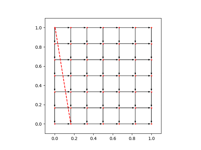
Figure 2: The distribution described in Example 1 is supported on the red segment (with $\delta=\nicefrac{{1}}{{6}}$). The Figure also represents the uniform grid for $\varepsilon=\nicefrac{{1}}{{6}}$.

We show how the instance in the example fools natural attempts to discretize the mechanisms space: the best mechanism in each one of these families has a multiplicative $\Theta(n)$ gap with respect to the expected revenue extracted by the best mechanism, thus invalidating the hope to achieve sublinear regret (even with respect to a constant fraction of the optimal revenue).

• Posted prices. A first parametric class of mechanisms is provided by posted prices, characterized by rectangular allocation regions. A mechanism in such class offers two prices, $p_{1}$ and $p_{2}$, and allocates if both agents accept. This is the immediate generalization of what happens for one agent. However, one can verify that the expected revenue of the best-fixed prices mechanism is $2^{-n}$ (ignoring the first agent who has an arbitrarily small valuation).

• Mechanisms on a grid. A more elaborate approach (similar to what is done, e.g., in Durvasula et al. (2023)) is to consider all the mechanisms whose allocation region can be described by the union of the tiles of a uniform grid (we formalize the class of grid mechanisms in Section 3; see Figure 3(a)). Surprisingly, this rich class is not more expressive than posted price mechanisms. It is always possible to set $\delta$ smaller or equal to the step size of the grid so that the whole distribution is supported on the first column (see Figure 2).

The Stochastic Algorithm: An Adaptive Grid.

The hard instance in Example 1 hints that we need an adaptive discretization. In particular, we show how to augment the class of mechanisms associated with uniform grids using the observed samples to approximate the revenue of the best mechanism while maintaining that the class is learnable. Our approach consists of adaptively refining the uniform grid tiles crossed by the boundary of the allocation region of the mechanism (see Figure 3(c) for a visualization). Both the learnability and the approximation properties of these class of “augmented grid” mechanisms build on a decomposition of the revenue function, which associates a weight to each edge of the grid and reduces the problem to finding a longest path. Besides achieving sublinear regret, our algorithm Augment-the-Best-Mechanism can be efficiently implemented. We mention that also the analysis of Csapó and Müller (2013) features a reduction to a graph problem; although somehow related, there the optimization goal is maximal closure, the decomposition is node-based, and the reduction critically needs finite support of the distribution.

The Smooth Algorithm: From Paths to Edges.

As observed, there is a natural class of mechanisms described by the $(0,1)$ to $(1,0)$ paths that are “down-right” in the uniform grid $G_{\varepsilon}$, where $\varepsilon$ is the step-size. A crucial observation is that assuming smoothness, the discretization error over $T$ rounds, i.e., the gap between the best mechanism and the best mechanism supported on $G_{\varepsilon}$ is of order $O(\varepsilon T)$ (Lemma 2). This can be shown by considering the best mechanism, observing through which tiles it passes, and considering the “inner hull” mechanism on the grid. This discretization is not enough to get an efficient algorithm with a good regret bound: crucially, in fact, the cardinality of the paths in $G_{\varepsilon}$ is still exponential in $\nicefrac{{1}}{{\varepsilon}}$. We observe that standard approaches to deal with large classes of experts either are not implementable (e.g., the Hedge algorithm (Arora et al., 2012), needs to maintain a weight for each one of the paths) or give bounds worse than our $O(T^{\nicefrac{{2}}{{3}}})$ (e.g., “follow the leader” approaches exhibit way worse bounds, see for instance Theorem 1.1. of Kalai and Vempala (2005) ). We overcome this problem by designing a careful sampling scheme that allows us to implement the Hedge algorithm efficiently; in particular, with an approach similar in spirit to Takimoto and Warmuth (2003), we maintain weights on the edges of $G_{\varepsilon}$ instead of its paths.

Lower Bounds.

Proving lower bounds in a structured and continuous environment is challenging, as it entails constructing hard instances while respecting the structure of the problem, i.e., points are valuations mapped to revenue via a specific function. In the lower bound for the stochastic and smooth adversary, we embed the standard hard instance for prediction with expert (Cesa-Bianchi and Lugosi, 2006) into a smooth distribution. For the adversarial lower bound, we use a needle in a haystack technique to construct an instance characterized by an optimal mechanism –the needle– that always makes the trade happen and extracts maximum profit from it, while no learning algorithm can extract more than half of the revenue at each iteration.

1.3 Further Related Work

(Online) Learning of Economic Problems

Following the seminal work of Kleinberg and Leighton (2003), there is a flourishing line of works that studies economic problems from an online learning perspective. For instance, the following problems have been studied: auctions from both the mechanism designer (e.g., Cesa-Bianchi et al., 2015; Roughgarden and Wang, 2019) and the bidders (e.g., Feng et al., 2018; Daskalakis and Syrgkanis, 2022; Cesa-Bianchi et al., 2024) perspective, bilateral trade (Azar et al., 2022; Cesa-Bianchi et al., 2023, 2023; Bernasconi et al., 2024; Babaioff et al., 2024), contracts (Ho et al., 2014; Zhu et al., 2023; Dütting et al., 2023), prophet inequalities (Gatmiry et al., 2024), brokerage (Bolic et al., 2024), and Bayesian persuasion (Castiglioni et al., 2023). With the exemption of Daskalakis and Syrgkanis (2022) and Ho et al. (2014); Zhu et al. (2023), the positive results in this line of work mostly pertain to cases where the object of learning is not complex. For example, Cesa-Bianchi et al. (2015) consider the problem of learning reserve prices (rather than optimal auctions), and the positive results in Zhu et al. (2023); Dütting et al. (2023) are for linear contracts which are defined through a single parameter. The results in Daskalakis and Syrgkanis (2022) and Ho et al. (2014); Zhu et al. (2023) for more complex objects are mostly impossibility results.

A closely related approach to learning in economic design problems considers the offline learning problem in the spirit of PAC-learning (e.g., Cole and Roughgarden, 2014; Morgenstern and Roughgarden, 2015). While there are known constructions that derive regret bounds for the online problem from sample complexity bounds for the offline problem, we are not aware of any prior work that would imply non-trivial results for our settings. For instance, Cole and Roughgarden (2014) consider an excludable setting where bidders’ valuations are independent and make regularity assumptions on the distribution; we consider a non-excludable setting with arbitrary distributions. Morgenstern and Roughgarden (2015) provide results only if the pseudo-dimension is finite; in Appendix A.1 we prove that such measure is unbounded in our problem. Guo et al. (2021) develop an approach that does not rely on any complexity measures of the hypothesis classes, and show general sample complexity bounds for product distributions. Their general bounds imply sample complexity bounds for a range of applications, via appropriate discretizations of the value space. In contrast, a main challenge in our problem is the lack of such discretization (see Example 1). Instead, our main result for the stochastic setting is driven by a non-trivial data-dependent discretization of the mechanism space (captured by a carefully designed infinite family of mechanisms, for which Theorem 3 provides a sample complexity bound).

Non-Excludable Mechanism Design.

Questions of non-excludable mechanism design are an active field of research. For example, Haghpanah et al. (2021) consider the problem of selling to a group where the payment of all group members has to be the same. This model is inspired by situations (e.g., a department purchasing some equipment) where there is only a single payment (to be made by the department), but all agents (members of the department) have different values for the item and need to agree on a purchase decision. Balseiro et al. (2021) tackle instead the design of dynamic mechanisms that exploit the repeated interaction with the same agents (think Cremer-McLean style full-surplus extraction); that work falls into a rather different territory than we do here.

2 The Learning Model

We formally describe the learning protocol for the Repeated Joint Ads problem. We also refer to the pseudocode for further details. At each time step $t=1,2,\dots,T$, a new pair of agents arrives, characterized by private valuations $(v^{t}_{1},v^{t}_{2})$ in the $[0,1]^{2}$ square. Independently, the learner proposes a mechanism $M^{t}$ to the agents, who then declare bids $(b_{1}^{t},b_{2}^{t})$. A mechanism $M^{t}$ is composed by a non-excludable allocation rule $x^{t}:[0,1]^{2}\to\{0,1\}$ and two payment functions $p_{1}^{t},p_{2}^{t}:[0,1]^{2}\to[0,1]$ that map bids to allocation, respectively payment. The revenue of mechanism $M^{t}$ at time $t$ is denoted with $\textsf{rev}_{t}(M^{t})$ and is defined as

$$\textsf{rev}_{t}(M^{t})=x^{t}(b^{t}_{1},b^{t}_{2})\cdot[p^{t}_{1}(b^{t}_{1},b^{t}_{2})+p^{t}_{2}(b^{t}_{1},b^{t}_{2})].$$

for time $t=1,2,\ldots$ do

     a new pair of agents arrives with (hidden) valuations $(v^{t}_{1},v_{2}^{t})\in[0,1]^{2}$

     the learner declares a mechanism $M^{t}\in\mathcal{M}$

     the agents declare their bids to the learner, allocation and payments are made accordingly

     the learner gains $\textsf{rev}_{t}(M^{t})$ (relatively to the bids)

Learning Protocol for the Repeated Joint Ads Problem

2.1 Structure of Incentive Compatible Mechanisms

The agents behave strategically, meaning that they strive to maximize their own quasi-linear utility $u^{t}_{i}(b_{1}^{t},b_{2}^{t})=v^{t}_{i}\cdot x^{t}(b_{1}^{t},b_{2}^{t})-p^{t}_{i}(b_{1}^{t},b_{2}^{t})$ for $i\in\{1,2\}$. To avoid unpredictable strategic misreporting from the agents, we require the mechanism $M^{t}$ proposed by the learner to enforce two properties:

• ex-post dominant strategy incentive compatibility (DSIC): regardless of the other’s bid, each agent maximizes its utility by being truthful. Formally, for any pair of actual valuations $(v_{1}^{t},v_{2}^{t})$ and possible bids $b_{1}$ and $b_{2}$ we have $u^{t}_{1}(v_{1}^{t},b_{2})\geq u^{t}_{1}(b_{1},b_{2})$ and $u^{t}_{2}(b_{1},v_{2}^{t})\geq u^{t}_{2}(b_{1},b_{2})$.

• ex-post individual rationality (IR): truthfulness never induces negative utility. Formally, for any actual valuations $(v_{1}^{t},v_{2}^{t})$ and possible bids $b_{1}$ and $b_{2}$ we have $u^{t}_{1}(v_{1}^{t},b_{2})\geq 0$ and $u^{t}_{2}(b_{1},v_{2}^{t})\geq 0.$

Our problem falls within the framework of single parameter auctions (Myerson, 1981), as each agent is characterized by a single value representing its value for the good for sale. This tells us that $(i)$ an allocation rule is implementable if and only if it is monotone and $(ii)$ for each such allocation rule there exists a unique payment rule that completes it to a DSIC and IR mechanism.

• monotone allocation rule: an allocation rule $x$ is monotone if for every bid $b_{1}$ and $b_{2}$, the two functions $x(z,b_{2})$ and $x(b_{1},z)$ are non-decreasing in $z$.

Given a monotone allocation rule $x$, the unique payment rule $p=(p_{1},p_{2})$ that completes it to a DSIC and IR mechanism can be computed via the critical prices, in particular (adopting the convention that the $\operatorname*{arg\,min}$ of the empty set is $0$) we have:

$$\begin{cases}p_{1}(b_{1},b_{2})=\operatorname*{arg\,min}\{\pi\in[0,1]\mid x(\pi,b_{2})=1\},\\ p_{2}(b_{1},b_{2})=\operatorname*{arg\,min}\{\pi\in[0,1]\mid x(b_{1},\pi)=1\}.\end{cases}$$

A Geometric View.

The notion of monotone allocation rule and the relative payments have a clean geometric interpretation in our setting: any DSIC and IR mechanism $M$ is identified by its allocation region $A_{M}=\{(v_{1},v_{2})\in[0,1]^{2}\mid x(v_{1},v_{2})=1\}.$ We say that a point $(w_{1},w_{2})$ dominates point $(v_{1},v_{2})$ if $w_{1}\geq v_{1}$ and $w_{2}\geq v_{2}$. To respect monotonicity $A_{M}$ has the following property: if $(v_{1},v_{2})\in A_{M}$, and $(w_{1},w_{2})\in[0,1]^{2}$ dominates it, then $(w_{1},w_{2})\in A_{M}$. We call a subset $A$ of $[0,1]^{2}$ monotone if such property is respected. A monotone region is enclosed by the sides of the $[0,1]^{2}$ square and a monotonically non-increasing curve that starts from either the north or the west side of the square and terminates into either the east or south side of it (see Figure 1). The total payment is then given by the sum of the orthogonal projections (horizontal and vertical) of the valuations onto the boundary of $A_{M}$. All in all, this allows us to forget about the strategic nature of the problem by characterizing mechanisms via “monotone” allocation regions (or their boundary) and implementing payments accordingly; for this reason, in the rest of the paper, there is no mention of bids as the agents always report their valuations truthfully. Similarly, we always intend mechanisms to be DSIC and IR.

Technical convention.

We make the technical assumption that allocation regions are always closed. This is without loss of generality as we are interested in revenue maximizing auctions and taking the closure of the allocation region may only increase the revenue. The assumption allows us, for instance, to use $\min$ instead of $\inf$ in the pricing rule and basically says that valuations belonging to the allocation region’s boundary result in an allocation.

2.2 Regret Minimization

The goal of the mechanism designer is to maximize its revenue over the $T$ rounds. In particular, the performance of a learning algorithm is measured in terms of its regret: the difference between the revenue achieved and that of the best fixed mechanism in hindsight. For any (possibly randomized) adversary $\mathcal{S}$ that generates the sequence of valuations, and learning algorithm $\mathcal{A}$, it is possible to define the regret of $\mathcal{A}$ against $\mathcal{S}$ as follows:

$$R_{T}(\mathcal{A},\mathcal{S})=\sup_{M\in\mathcal{M}}\mathbb{E}\left[\sum_{t=1}^{T}\textsf{rev}_{t}(M)-\sum_{t=1}^{T}\textsf{rev}_{t}(M^{t})\right].$$

The mechanisms $M_{t}$ are proposed by the learning algorithm $\mathcal{A}$, while the agents’ valuations are generated by the adversary $\mathcal{S}$. $\mathcal{M}$ denotes the class of all the DSIC and IR mechanisms. The expectation in the above formula is with respect to the internal randomness of $\mathcal{A}$ and (possibly) of $\mathcal{S}$. The goal of the learner is to design an algorithm $\mathcal{A}$ with small regret over all the possible adversaries: $R_{T}(\mathcal{A})=\sup_{\mathcal{S}}R_{T}(\mathcal{A},\mathcal{S})$. We consider three models of adversaries:

• In the (oblivious) adversarial setting, an adversary generates the sequence of valuations $\{(v_{1}^{t},v_{2}^{t})\}$ up-front in an arbitrary way.

• In the stochastic setting, the valuations are drawn i.i.d. from an unknown and possibly correlated but fixed distribution.

• In the $\sigma$-smooth setting, an adversary chooses a sequence of $\sigma$-smooth random variables $V^{t}=(V_{1}^{t},V_{2}^{t})$ from which the actual valuations $v^{t}=(v_{1}^{t},v_{2}^{t})$ are drawn from. We say that a random variable is $\sigma$-smooth if its distribution is $\sigma$-smooth as defined below.

Definition 1 (Haghtalab et al. (2021)).

Let $X$ be a domain supporting a uniform distribution $\nu$. A measure $\mu$ on $X$ is $\sigma$-smooth, for some $\sigma\in(0,1]$, if for all measurable $A\subseteq X$, we have $\mu(A)\leq\frac{\nu(A)}{\sigma}$.

3 The Stochastic Upper Bound

In this section, we present an (efficient) learning algorithm, Augment-the-Best-Mechanism, which exhibits a $\tilde{O}(T^{3/4})$ upper bound on the regret. First, in Section 3.1, we introduce the family of orthogonal mechanisms that well approximate the whole class of mechanisms for the Joint Ads Problem. Second, in Section 3.2, we present a data-dependent discretization scheme focusing on a learnable subfamily of orthogonal mechanisms that retain their approximating power. Finally, in Section 3.3, we discuss how to combine these ingredients in our algorithm.

3.1 From Revenues to Distances on a Graph: The Power of Orthogonal Mechanisms

Given the theory of single parameter auctions, to which our problem belongs, any DSIC and IR mechanism $M$ for the Joint Ads Problem is characterized by its allocation region $A_{M}$. The first natural attempt to discretize such action space is to consider allocation regions that can be seen as a union of tiles in a uniform grid; however, we know that such a class is not rich enough to successfully approximate the best mechanism (see the discussion after Example 1). To overcome this, we introduce a generalization of such a family, the class of orthogonal mechanisms.

Definition 2 (Orthogonal Mechanisms).

A DSIC and IR mechanism $M$ is said to be orthogonal if its allocation region’s boundary is composed of a finite union of vertical and horizontal segments. We denote the class of all orthogonal mechanisms with $\mathcal{M}^{\perp}$.

Such mechanisms have a natural interpretation as “south-east” paths in a suitable class of graphs.

Definition 3 (Orthogonal Graphs).

A directed graph $G=(V,E)$ is said to be orthogonal if:

• Each vertex $u\in V$ is a distinct point $(u_{1},u_{2})\in[0,1]^{2}$.

• There is a unique source $s=(s_{1},1)\in V$ and a unique sink $t=(1,t_{2})\in V$.

• Each edge $e=(u,v)\in E$ is either vertically pointing down-wards ($u_{1}=v_{1}$ and $u_{2}>v_{2}$) or horizontally pointing right-wards ($u_{1}<v_{1}$ and $u_{2}=v_{2}$), and the segments representing edges may only intersect in their endpoints.

• Each node in $V\setminus\{s,t\}$ has at least an incoming and an outgoing edge.

We say that a path $\pi$ in $G$ from vertex $w$ to vertex $v$ is complete if $w$ belongs to the north side of the square ($w_{2}=1$) and $v$ belongs to the east side of it ($v_{1}=1$).

Property (iv) guarantees that any maximal path starting from a node on the north side of the square terminates on the east side of it (and is thus complete). Furthermore, any orthogonal graph $G$ is acyclic by property (iii). For any complete path $\pi$ in an orthogonal graph, it is natural to identify the mechanism $M_{\pi}$ whose allocation region falls on the “top-right” part of the square with respect to $\pi$. Formally, valuation $(v_{1},v_{2})$ is in the allocation region of $M_{\pi}$ if there exists a node $u=(u_{1},u_{2})$ in $\pi$ such that $v_{1}\geq u_{1}$ and $v_{2}\geq u_{2}$. We refer to the Figure 3(a) for a visualization: the allocation region of the orthogonal mechanism is shaded in blue, while the path representing its boundary is red. The relation between orthogonal graphs and mechanisms is explicit in the following Proposition.

Proposition 1.

Let $G=(V,E)$ be any orthogonal graph, and $\pi$ any complete path in $G$, then $M_{\pi}\in\mathcal{M}^{\perp}$. Conversely, for any $M\in\mathcal{M}^{\perp}$, there exists a complete path $\pi$ in some orthogonal graph such that $M=M_{\pi}$.

Proof.

Fix any orthogonal graph $G$ and complete path $\pi$ in it, and consider the associated mechanism $M_{\pi}$, which is the mechanism associated by the allocation region $A_{\pi}$ of all the points that dominate at least a node in $\pi$. Regarding the shape of $A_{\pi}$, its boundary is given by the union of the edges in $\pi$ (which are either horizontal or vertical by definition of orthogonal graphs) and possibly portions of the north or east side of the $[0,1]^{2}$ square. We must also formally prove that $A_{\pi}$ is monotone. Let $(v_{1},v_{2})\in A_{\pi}$ and $(w_{1},w_{2})$ any point that dominates it, then also $(w_{1},w_{2})\in A_{\pi}$ because, by definition of $M_{\pi}$ there exists $u=(u_{1},u_{2})$ in $\pi$ such that $w_{1}\geq v_{1}\geq u_{1}$ and $w_{2}\geq v_{2}\geq u_{2}$.

The converse is easy to prove: fix any orthogonal mechanism $M\in\mathcal{M}^{\perp}$ and consider the part of the boundary of $A_{M}$ that goes from the north to the east side of the square; by definition, such curve is the union of vertical and horizontal segments. Thus, it constitutes a path that respects the properties of an orthogonal graph. ∎

For this reason, we can safely identify complete paths on orthogonal graphs with the corresponding orthogonal mechanisms and orthogonal graphs $G$ with the family of orthogonal mechanisms that complete paths of $G$ can describe. The relation between these two concepts goes even further: the revenue of any orthogonal mechanism is equal to the sum of carefully chosen weights on the associated path.

Definition 4 (Edge weights).

Fix any orthogonal graph $G$ and any edge $e$ in it. We define its influence region $A_{e}$ and intrinsic weight $w_{e}$ as follows:

$$\begin{cases}A_{e}=[x,1]\times[u_{2},v_{2})\text{ and }w_{e}=x\text{ if $e=(u,v)$ with $u_{1}=v_{1}=x$}\\ A_{e}=[u_{1},v_{1})\times[y,1]\text{ and }w_{e}=y\text{ if $e=(u,v)$ with $u_{2}=v_{2}=y$}\end{cases}$$

where we adopt the convention that if $v_{2}=1$ in the first case or $v_{1}=1$ in the second case, then the corresponding interval extreme is closed. Fix now any random variable $V=(V_{1},V_{2})$ on $[0,1]^{2}$, we define the weight function $w_{V}:E\to[0,1]$ as $w_{V}(e)=w_{e}\cdot\mathbb{P}\left(V\in A_{e}\right).$

Stated differently, we associate to each edge $e$ its contribution to the revenue if such edge belongs to the path associated with the orthogonal mechanism. (See Figure 3(b) for a visualization of the allocation regions $A_{e}$, in red for a vertical edge and blue for a horizontal one).

Proposition 2.

Consider any random variable $V$ in $[0,1]^{2}$ describing the agents’ valuations, and any orthogonal graph $G=(V,E)$, then for any complete path $\pi$ in $G$ it holds that

$$\mathbb{E}\left[\textsf{rev}(M_{\pi})\right]=\sum_{e\in\pi}w_{V}(e)=\sum_{e\in\pi}w_{e}\cdot\mathbb{P}\left(V\in A_{e}\right).$$

Proof.

We start by considering the payment made by the first agent. Agent $1$ pays if and only if the valuation $(v_{1},v_{2})$ falls into the allocation region, partitioned by all the $A_{e}$ for $e$ vertical edges in $\pi$. If the valuation falls into $A_{e}$, then the price paid by agent $1$ is computed according to Myerson’s rule and is set precisely to $w_{e}$. All in all, the revenue extracted by the first agent is exactly the sum over all the vertical edges in $\pi_{e}$ of $w_{e}\mathbb{P}\left(V\in A_{e}\right)$. A similar argument can be carried over for agent $2$ and the horizontal edges, thus proving the statement. Note that the edges that belong to the west and south sides of the square carry no weight. ∎

The previous proposition allows us to “discretize” the task of computing the revenue-maximizing mechanism. Given an orthogonal graph $G$, it is possible to calculate its best mechanism by simply computing the longest complete path. We can say something more; if the underlying distribution is finitely supported, then it is possible to create an orthogonal graph (whose node set is composed of the grid generated by the points in the support and thus contains them) that is guaranteed to contain an optimal mechanism on one of its paths, therefore allowing for efficient recovery of the optimal mechanism.

Theorem 1.

Consider any finitely-supported random variable $V$ in $[0,1]^{2}$ describing the agents’ valuations, then there exists an orthogonal mechanism $M^{\star}\in\mathcal{M}^{\perp}$ that can be computed efficiently (in $|supp(V)|$) that is revenue maximizing:

$$\mathbb{E}\left[\textsf{rev}(M^{\star})\right]\geq\mathbb{E}\left[\textsf{rev}(M)\right],\,\forall M\in\mathcal{M}.$$

Proof.

First, we prove that we can restrict our attention to study mechanisms whose allocation region is minimal with respect to the inclusion. Second, we fix any such mechanism $M$ and prove that it is indeed orthogonal. Finally, we explain how to efficiently compute such $M^{\star}$.

We start with the first step. Fix any mechanism $M$, and consider the auxiliary mechanism $M^{\prime}$ characterized by the following allocation region:

$$A_{M^{\prime}}=\{(w_{1},w_{2})\in[0,1]^{2}\mid\exists(v_{1},v_{2})\in\mathrm{supp}(V)\cap A_{M}\text{ s.t. }w_{1}\geq v_{1}\text{ and }w_{2}\geq v_{2}\}.$$

$A_{M^{\prime}}$ contains all points that are dominated by the valuations in $supp(V)$ that also belong to $A_{M}$.

Claim 1.

$A_{M^{\prime}}$ is the monotone region that contains $\mathrm{supp}(V)\cap A_{M}$ which is minimal with respect to inclusion. Therefore $A_{M^{\prime}}\subseteq A_{M}$ and $\mathbb{E}\left[\textsf{rev}(M^{\prime})\right]\geq\mathbb{E}\left[\textsf{rev}(M)\right]$.

Proof of 1.

For any $(u_{1},u_{2})\in A_{M^{\prime}}$ there exists a $(v_{1},v_{2})\in\mathrm{supp}(V)\cap A_{M}$ which dominates it. But such $(v_{1},v_{2})$ belongs to $A_{M}$ which is monotone, so $(u_{1},u_{2})$ has to belong to $A_{M}$ by monotonicity. Minimality follows by the same argument. Since $A_{M}$ contains $A_{M}^{\prime}$, it immediately holds that $\mathbb{E}\left[\textsf{rev}(M^{\prime})\right]\geq\mathbb{E}\left[\textsf{rev}(M)\right]$, as increasing the size of the allocation region without changing the intersection with the support of $V$ only causes the payment to decrease. ∎

We move to the second part of the proof: any mechanism $M$ whose allocation region is minimal with respect to inclusion is orthogonal. The intuition is that any “curve” part of the boundary is not inclusion-minimal and can be rectified without affecting the points in the support of $V$ covered.

Claim 2.

Any mechanism $M$ whose allocation region is minimal with respect to inclusion with respect to a subset of $\mathrm{supp}(V)$ is orthogonal.

Proof of 2.

Let $S_{x}$ be the set of all the values of the first coordinates of the points in $\mathrm{supp}(V)\cap A_{M}$ union $\{0,1\}$, and let $S_{y}$ be the analogous set for the second coordinate. We introduce the orthogonal graph $G$ whose vertex set is given by the grid $S_{x}\times S_{y}$, and each vertex is linked by a directed edge to the closest nodes on the right and on the bottom (if any). Consider now the set of vertices $S_{M}$ that belongs to the grid $S_{x}\times S_{y}$ and to the allocation region $A_{M}$. By monotonicity of $A_{M}$, $S_{M}$ is connected and respects a “discrete” monotonicity property: if $u$ is in $S_{M}$ and $v$ is a generic node of $G$ that dominates $u$, then $v$ is in $S_{M}$. Consider now the (Pareto) frontier of $S_{M}$: all the points $(u_{1},u_{2})\in S_{M}$ that do not strictly dominate other points in $S_{M}$. More precisely, $u\in S_{M}$ belongs to the frontier of $S_{M}$ if $\not\exists w\in S_{M}$ such that $u_{1}>w_{1}$ and $u_{2}>w_{2}$. We prove that the path $\pi$ composed by the points on the frontier of $S_{M}$ is such that $M=M_{\pi}$ (note, $M_{\pi}$ is orthogonal by Proposition 1). In particular, we prove that $A_{M}=A_{M_{\pi}}$. One inclusion is easy: $A_{\pi}$ contains $\mathrm{supp}(V)\cap A_{M}$ and therefore is contained in $A_{M}$ because of its minimality (1). Consider now any $u\in A_{\pi}$, we want to prove that it belongs to $A_{M}$. Point $u$ is in $A_{\pi}$, therefore there exists $v\in\pi$ which is dominated by it, but $v$ also belong to $A_{M}$ and thus $u\in A_{M}$ by monotonicity. ∎

We are left with the final step of our proof, that concerns presenting an efficient algorithm to find $M^{\star}$: the revenue maximizing mechanism that is also orthogonal. First we observe that the support of $V$ is finite, therefore there exists a finite number of subsets of points that can be included in the allocation region. To each of these subsets we can associate the inclusion minimal mechanism, which is revenue maximizing and orthogonal (by Claims 1 and 2). Consider now the orthogonal graph whose node set is composed by the Cartesian product of the $x$ and $y$ coordinates of all the points on the support of $V$ (and the edges are constructed similarly to what we did in the proof of 2); this graph will contain as subgraph the one used in the proof of 2 for the optimal subset of the support of $V$, so it is enough to find the best orthogonal mechanism supported on such graph. By Proposition 2, this is equivalent to finding the maximum weight complete path in $G$. This task can be done efficiently (i.e., in time polynomial in the cardinality of the support of $V$) by running the Belman-Ford algorithm that solves the shortest path problem on the same graph but where the costs are $c(e)=-w_{V}(e)$. In particular, one needs to compute the shortest path between any pair of north-east side points that can be the extreme of a complete path. Note, $G$ is acyclic so the algorithm converges to the optimum. ∎

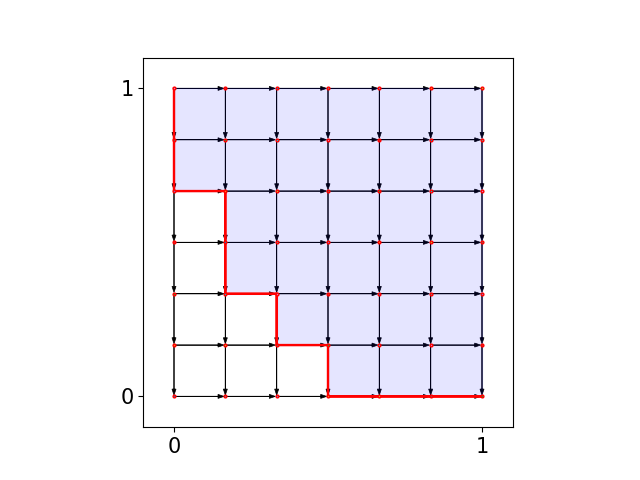
(a) An orthogonal graph: $G_{\nicefrac{{1}}{{6}}}$

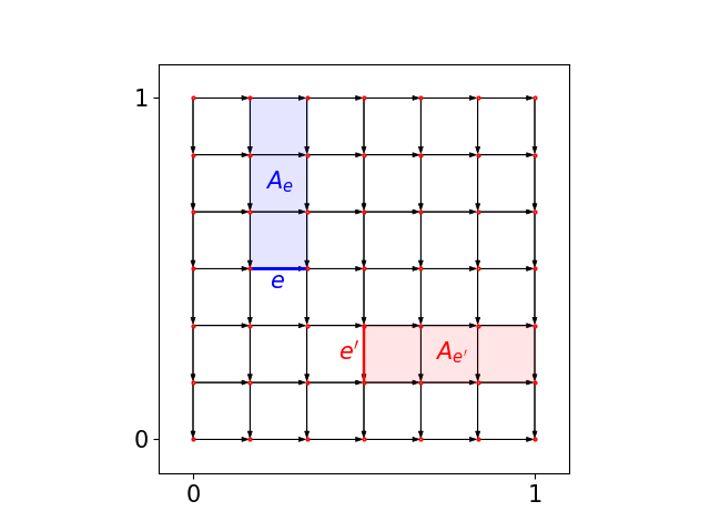
(b) Influence regions for $e$ and $e^{\prime\prime}$

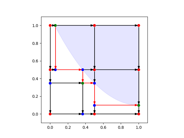
(c) Augmentation Procedure

Figure 3: An orthogonal graph (left) and the rectangles $A_{e}$ for vertical and horizontal edges (center). Note that while the two figures are for a uniform grid, this is not needed for orthogonal mechanisms. On the right, there is a visualization of the augmentation procedure: $G_{\nicefrac{{1}}{{2}}}$ (red nodes) is augmented with the three green points (note the auxiliary points in blue). These points have been chosen to mimic the procedure used in Lemma 1 to approximate the mechanism whose allocation region is shaded in blue with the orthogonal one corresponding to the red complete path.

3.2 A (Learnable) Data-Dependent Discretization Scheme

From an online learning perspective, Theorem 1 allows us to efficiently compute the best mechanism on the empirical distribution of the valuations seen so far in a Follow-The-Leader way. However, this would not yield a meaningful algorithm, as both the class $\mathcal{M}$ and even the subclass of orthogonal mechanisms $\mathcal{M}^{\perp}$ seem too complex for the revenue function to be learned efficiently (this is witnessed for instance, by the fact that $\mathcal{M}^{\perp}$ has unbounded pseudo-dimension, see Section A.1). As an intermediate step, we formally introduce a natural subfamily of the orthogonal graphs: the uniform grids (see also the second bullet after Example 1).

Definition 5 (Uniform Grid).

For any $\varepsilon>0$, we define the uniform grid graph $G_{\varepsilon}=(V_{\varepsilon},E_{\varepsilon})$:

• $V_{\varepsilon}=\{0,{\varepsilon},2\varepsilon,\ldots,1\}^{2}$

• $E_{\varepsilon}$ connects each point of the grid to its right and bottom neighbor (if any).

For instance, the graph depicted in Figure 3(a) is $G_{\nicefrac{{1}}{{6}}}.$ For any fixed $\varepsilon$, the family $\mathcal{M}_{\varepsilon}$ of all the mechanisms that are induced by complete paths in $G_{\varepsilon}$ has the desirable property that its revenue function can be learned quickly, as we only need to learn the weight function $w_{V}$ on the $\Theta(\nicefrac{{1}}{{\varepsilon^{2}}})$ edges (by Proposition 2). However, as we observed in Example 1, for any fixed $\varepsilon$, there exists a simple distribution $V$ such that the revenue of the best fixed mechanism in $\mathcal{M}_{\varepsilon}$ is far from that of the best mechanism in $\mathcal{M}$. We are thus in a situation where the large family of orthogonal mechanisms well approximates the optimal mechanism, but it is unclear whether it can be learned effectively. In contrast, mechanisms supported on uniform grids have revenue functions that are easy to learn but may exhibit a big gap with respect to the performance of the best mechanism overall. To escape this situation, we next describe a class of mechanism that is only slightly larger than the former class, and (approximately) retains the approximation property of the latter class.

For any $\varepsilon$, the grid $G_{\varepsilon}$ partitions the $[0,1]^{2}$ square into $\nicefrac{{1}}{{\varepsilon^{2}}}$ tiles of area $\varepsilon^{2}$ (out of simplicity, we often implicitly assume that $\nicefrac{{1}}{{\varepsilon}}$ is integer, this does not hinder the general validity of our results). Consider now one of these tiles, let’s say the one whose top left vertex is $(i\varepsilon,j\varepsilon)$ and a point $(v_{1},v_{2})$ inside such tile. To avoid overlapping, we do not consider the south and west sides of each tile, so that $i\varepsilon<v_{1}\leq(i+1)\varepsilon$ and $(j-1)\varepsilon<v_{2}\leq j\varepsilon$. We show a procedure to incorporate point $(v_{1},v_{2})$ into its tile (and thus into $G_{\varepsilon}$) while retaining the orthogonality of the overall graph. We call the outcome of this procedure as $G_{\varepsilon}$ augmented with point $(v_{1},v_{2})$. We have four cases:

• If $(v_{1},v_{2})$ belongs to the interior of the tile, i.e., $i\varepsilon<v_{1}<(i+1)\varepsilon$ and $(j-1)\varepsilon<v_{2}<j\varepsilon$, then we add $(v_{1},v_{2})$ and four other nodes to the node set of of $G_{\varepsilon}$: $(v_{1},j\varepsilon)$, $(v_{1},(j-1)\varepsilon)$, $(i\varepsilon,v_{2})$ and $((i+1)\varepsilon,v_{2})$. Then we add an edge between each one of these nodes and $(v_{1},v_{2})$, respecting the right-down direction. The four nodes added belong to the sides of the tile, so, to maintain orthogonality, we split such edges in two: for instance, let $e=(u,z)$ be the edge containing node $w\in\{(v_{1},j\varepsilon),(v_{1},(j-1)\varepsilon),(i\varepsilon,v_{2}),((i+1)\varepsilon,v_{2}))$, then we remove $e$ from the edge set, and we insert $e^{\prime}=(u,w)$ and $e^{\prime\prime}=(w,z)$ in its place (south-west tile in Figure 3(c)).

• If $(v_{1},v_{2})$ belongs to a vertical edge $e=(u,w)$, then we only add two nodes: $(v_{1},v_{2})$ and $(i\varepsilon,v_{2})$, we split the corresponding vertical edges and add a horizontal edge between them (south-east tile in Figure 3(c)).

• If $(v_{1},v_{2})$ belongs to a horizontal edge, $e=(u,w)$, then we only add two nodes: $(v_{1},v_{2})$ and $(v_{1},j\varepsilon)$, we split the corresponding horizontal edges and add a vertical edge between them (north-west tile in Figure 3(c)).

• If $(v_{1},v_{2})$ is already a vertex of the graph, we do nothing.

We can apply this augmentation property recursively for a subset $S$ of points, at the condition that at most one node appears in any tile of the original grid $G_{\varepsilon}$. Note, it is possible that edges of the original grid $G_{\varepsilon}$ may be split in more than two edges, as, e.g., the $(0,\nicefrac{{1}}{{2}})$-$(\nicefrac{{1}}{{2}},\nicefrac{{1}}{{2}})$ edge in Figure 3(c). We define the resulting orthogonal graph as the augmented grid graph $G_{\varepsilon,S}$ and denote with $M_{\varepsilon,S}$ the corresponding orthogonal mechanism. We then have the following definition:

Definition 6 (Augmented-Grid Mechanisms).

For any $\varepsilon>0$, we define the family of Augmented-Grid Mechanisms $\hat{\mathcal{M}}_{\varepsilon}$ as all the orthogonal mechanisms $M_{\varepsilon,S}$ for some set of points $S$, with $|S|\leq\nicefrac{{2}}{{\varepsilon}}$.

Surprisingly enough, adding only this small amount of points ($\Theta(\nicefrac{{1}}{{\varepsilon}})$ many) gets the best of both the orthogonal and the grid mechanisms, achieving approximation and learnability! This is proved in the following Lemma. Starting from any mechanism $M$, it is possible to construct an augmented grid mechanism that well approximates $M$. The procedure is depicted in Figure 3(c) and consists of adapting the tiles of $G_{\varepsilon}$ that contain the border of the allocation region to mimic the behavior of $A_{M}$.

Lemma 1.

Fix any $\varepsilon>0$ and any random variable $V$ in $[0,1]^{2}$ describing the agents’ valuations. For any mechanism $M\in\mathcal{M}$, there exists an augmented-grid mechanism $\hat{M}\in\hat{\mathcal{M}}_{\varepsilon}$ such that

$$\mathbb{E}\left[\textsf{rev}({M})\right]\leq\mathbb{E}\left[\textsf{rev}({\hat{M}})\right]+2\varepsilon$$

Proof.

Let $M$ be any mechanism, and consider its allocation region $A_{M}$. If $A_{M}$ is the union of tiles of $G_{\varepsilon}$, then there is nothing to prove, as $M$ is then orthogonal. We then focus on all the tiles of $G_{\varepsilon}$ that lie at the boundary of $A_{M}$, i.e., that intersect $A_{M}$ but are not entirely contained in it; these are the tiles we augment. These tiles are at most $\nicefrac{{2}}{{\varepsilon}}$, so the output of this procedure belongs to $\hat{\mathcal{M}}_{\varepsilon}$, as requested in the statement.

Consider any one of these tiles, and the intersections $u$ and $v$ of the boundary of the allocation region with the sides on the tile.. We have various cases:

• If $u$ belongs to the north side and $v$ to the east side, then we augment the tile with $(u_{1},v_{2})$ (see south-west tile of Figure 3(c))

• If $u$ belongs to the north side and $v$ to the south side, then we augment the tile with $u$ (see north-west tile of Figure 3(c))

• If $u$ belongs to the east side and $v$ to the west one, then we augment the tile with $v$ (see south-east tile of Figure 3(c))

• Otherwise we do not augment the tile

Consider now the minimal complete path $\pi$ on the augmented graph with the property that $A_{\pi}$ contains $A_{M}$. As $A_{\pi}$ contains $A_{M}$, the orthogonal mechanism always trades when $M$ does it. Conversely, for any valuation $v\in A_{M}$ the projections on $\pi$ and the boundary of $A_{M}$ belong to the same tile!, therefore the prices proposed by the orthogonal mechanism are at most an additive $\varepsilon$ term smaller than the ones charged by $A_{M}$. This concludes the proof. ∎

For any $M\in\mathcal{M}$, we refer to the mechanism $\hat{M}$ of Lemma 1 as the associated augmented-grid mechanism with precision $\varepsilon$. An immediate consequence of Lemma 1 is that the best mechanism in $\hat{\mathcal{M}}_{\varepsilon}$ is only an additive $\Theta(\varepsilon)$ factor away from the optimal mechanism.

Theorem 2.

Fix any $\varepsilon>0$ such that $\nicefrac{{1}}{{\varepsilon}}\in\mathbb{N}$ and any random variable $V$ in $[0,1]^{2}$ describing the agents’ valuations, then there exists $\hat{M}\in\hat{\mathcal{M}}_{\varepsilon}$ such that

$$\sup_{M\in\mathcal{M}}\mathbb{E}\left[\textsf{rev}({M})\right]-\mathbb{E}\left[\textsf{rev}(\hat{M})\right]\leq 3\varepsilon.$$

We move our attention to learnability. We exploit the edge-decomposition of the revenue function (Proposition 2) to argue that, to achieve an $\varepsilon$-precise approximation of the revenue function on all the mechanisms in $\hat{\mathcal{M}}_{\varepsilon}$, it is enough to achieve an $\varepsilon^{2}$ approximation of all the rectangles in the $[0,1]^{2}$ square (as any path contains $O(\nicefrac{{1}}{{\varepsilon}})$ edges and each edge $e$ is associated to a rectangular region $A_{e}$). Since the range space of all the rectangles has constant VC dimension, $n\in\tilde{\Omega}(\nicefrac{{1}}{{\varepsilon^{4}}})$ samples are sufficient.

Theorem 3.

Fix any failure probability $\delta\in(0,\nicefrac{{1}}{{2}})$ and precision $\varepsilon>0$, and let $V_{1},V_{2},\dots,V_{n}$ be $n$ i.i.d. samples from the random variable $V$ describing the agents valuations. If $n\geq\tfrac{256}{\varepsilon^{4}}\left(32\log\tfrac{8}{\varepsilon}+\log\tfrac{2}{\delta}\right)$, then the following holds with probability at least $1-\delta$:

$$|\hat{\mathbb{E}}[\textsf{rev}(M)]-\mathbb{E}\left[\textsf{rev}(M)\right]|\leq\varepsilon,\,\forall M\in\hat{\mathcal{M}}_{\varepsilon},$$

where $\hat{\mathbb{E}}$ denotes the expectation with respect to the empirical distribution on the $n$ samples.

Proof.

For any mechanism $\mathcal{M}\in\hat{\mathcal{M}}_{\varepsilon}$ let $\mathcal{E}_{M}$ be the event that the empirical revenue of $M$ on the $n$ samples is $\varepsilon$ close to the actual one:

$$\mathcal{E}_{M}=\{|\hat{\mathbb{E}}[\textsf{rev}(M)]-\mathbb{E}\left[\textsf{rev}(M)\right]|\leq\varepsilon\}.$$

Let $\pi_{M}$ be the path in the grid-augmented graph associated with the boundary of $M$. Crucially, $\pi_{M}$ contains at most $\nicefrac{{4}}{{\varepsilon}}$ edges, this is because complete paths on $G_{\varepsilon}$ have cardinality at most $\nicefrac{{2}}{{\varepsilon}}$, and each added point adds at most $2$ edges each. If we exploit the decomposition result of Proposition 2, we can rewrite the difference between the two revenues as follows:

$$|\hat{\mathbb{E}} [\textsf{rev}(M)]-\mathbb{E}\left[\textsf{rev}(M)\right]|=|\sum_{e\in\pi_{M}}w_{e}(\hat{\mathbb{P}}(V\in A_{e})-\mathbb{P}\left(V\in A_{e}\right))|$$

$$\leq\sum_{e\in\pi_{M}}w_{e}|\hat{\mathbb{P}}(V\in A_{e})-\mathbb{P}\left(V\in A_{e}\right)|\leq\frac{4}{\varepsilon}\cdot\max_{e\in\pi_{M}}|\hat{\mathbb{P}}(V\in A_{e})-\mathbb{P}\left(V\in A_{e}\right)|.$$ (1)

So the problem has reduced to bounding the error on the class of all the axis-aligned rectangles of the form $A_{e}$ for some $e.$ Such class has VC dimension of $4$, so by standard learning arguments (e.g., Theorem 14.15 of Mitzenmacher and Upfal (2005)) and by our choice of $n$ we get that, with probability at least $1-\delta$, it holds $\max_{e\in\pi_{M}}|\hat{\mathbb{P}}(V\in A_{e})-\mathbb{P}\left(V\in A_{e}\right)|\leq\frac{\varepsilon^{2}}{4}.$ Plugging this into Equation 1 yields the desired result. ∎

3.3 The Augment-the-Best-Mechanism Algorithm

We have all the ingredients to present and analyze our learning algorithm: Augment-the-Best-Mechanism. At a generic time $t$, it computes $M^{\star}_{t}$, the revenue-maximizing mechanism over the $t-1$ valuations observed so far (note, this can be done efficiently because of Theorem 1) and then posts the associated grid-augmented mechanism $M^{t}$ for a suitable precision parameter $\varepsilon_{t}$. We refer to the pseudocode for further details. Given $M^{\star}_{t}$ it is easy to compute the associated augmented mechanism by following the procedure described in Lemma 1 and visualized in Figure 3(c).

Environment: Fixed random variable $V$ from which valuations $\{(v_{1}^{t},v_{2}^{t})\}$ are drawn i.i.d.

Propose any mechanism $M^{1}$ and observe $(v^{1}_{1},v_{2}^{1})$

for time $t=2,\ldots,T$ do

     Set precision parameter $\varepsilon_{t}=14\sqrt[4]{\nicefrac{{\log T}}{{t}}}$

     Let $M^{\star}_{t}$ be the revenue-maximizing mechanism over valuations $(v^{1}_{1},v_{2}^{1}),\dots,(v^{t-1}_{1},v_{2}^{t-1})$

     Let $M^{t}\in\hat{\mathcal{M}}_{\varepsilon}$ be the grid-augmented mechanism with precision $\varepsilon$ associated with $M^{\star}_{t}$

     Propose mechanism $M^{t}$ and observe $(v^{1}_{t},v_{2}^{t})$

Augment-the-Best-Mechanism

Theorem 4.

Consider the Repeated Joint Ads problem in the stochastic i.i.d. setting; then, there exists a learning algorithm $\mathcal{A}$ such that

$$R_{T}(\mathcal{A})\leq 35\sqrt[4]{T^{3}\cdot\log T}.$$

Proof.

We prove that Augment-the-Best-Mechanism yields the desired regret bound in the stochastic case. For all $t=2,\dots,T$, we denote with $\mathcal{E}_{t}$ the event that all the mechanisms in $\hat{\mathcal{M}}_{\varepsilon_{t}}$ are well approximated by the first $t-1$ samples:

$$\mathcal{E}_{t}=\left\{|\hat{\mathbb{E}}_{t-1}[\textsf{rev}(M)]-\mathbb{E}\left[\textsf{rev}(M)\right]|\leq\varepsilon_{t},\,\forall M\in\hat{\mathcal{M}}_{\varepsilon_{t}}\right\},$$

where $\hat{\mathbb{E}}_{t-1}$ denotes the empirical expectation with respect to the first $t-1$ samples. By our choice of $\varepsilon_{t}$ and Theorem 3, we have that the $\mathcal{E}_{t}$ are realized with high probability, i.e.,

$$\mathbb{P}\left(\mathcal{E}_{t}\right)\geq 1-\nicefrac{{1}}{{T}}.$$ (2)

Now focus on what happens at time $t$, conditioning on $\mathcal{E}_{t}$ happening. We have:

$$\sup_{M\in\mathcal{M}}\mathbb{E}\left[\textsf{rev}_{t}(M)\right] \leq\mathbb{E}\left[\textsf{rev}_{t}(\hat{M})\right]+3\varepsilon_{t} \hat{M}\in\hat{\mathcal{M}}_{\varepsilon_{t}}$$ (for some , by Theorem 2)

$$\leq\hat{\mathbb{E}}_{t-1}[{\textsf{rev}_{t}(\hat{M})}]+4\varepsilon_{t} \mathcal{E}_{t}$$ (Conditioning on )

$$\leq\hat{\mathbb{E}}_{t-1}[{\textsf{rev}_{t}(M_{t}^{\star})}]+4\varepsilon_{t} M_{t}^{\star} \hat{\mathbb{E}}_{t}$$ (By optimality of w.r.t. )

$$\leq\hat{\mathbb{E}}_{t-1}[{\textsf{rev}_{t}(M^{t})}]+6\varepsilon_{t} M^{t}$$ (By definition of and Lemma 1)

$$\leq{\mathbb{E}}[{\textsf{rev}_{t}(M^{t})}]+7\varepsilon_{t} \mathcal{E}_{t}$$ (Conditioning on )

Combining this chain of inequality with the bound on the probability of $\mathcal{E}_{t}$ in Equation 2, we get that the instantaneous regret suffered by Augment-the-Best-Mechanism is at most:

$$\sup_{M\in\mathcal{M}}\mathbb{E}\left[\textsf{rev}_{t}(M)\right]-\mathbb{E}\left[\textsf{rev}_{t}(M^{t})\right]\leq\left(7\varepsilon_{t}+\frac{2}{T}\right)\leq 8\varepsilon_{t}.$$

Overall, the regret is upper bounded by $8\sum_{t=1}^{T}\varepsilon_{t}$, which verifies the bound in the statement. ∎

4 Adversarial Lower Bound

We prove a lower bound on the regret when the sequence of valuations is generated adversarially. In particular, we show a stronger result: for any $\varepsilon$, no learning algorithm suffers sublinear $(2-\varepsilon)$-regret.

Theorem 5.

For any constant $\varepsilon\in(0,1)$ and learning algorithm $\mathcal{A}$, there exists an adversarial instance of the Repeated Joint Ads problem such that the following inequality holds:

$$\sup_{M\in\mathcal{M}}\sum_{t=1}^{T}\textsf{rev}_{t}(M)-(2-\varepsilon)\sum_{t=1}^{T}\mathbb{E}\left[\textsf{rev}_{t}(M_{t})\right]\geq\frac{\varepsilon^{2}}{8}T.$$

Proof.

Let $\delta$ and $\zeta$ be small positive parameters we set later. We prove this lower bound via Yao’s minimax principle: we construct a randomized instance against which any deterministic algorithm suffers expected linear $(2-\varepsilon)$ regret. The randomized instance is built incrementally, together with an auxiliary sequence $(a_{t},b_{t})$, as follows: $a_{1}=\nicefrac{{\delta}}{{3}}$, $b_{1}=\nicefrac{{2\delta}}{{3}}$, then for any time step $t$:

• with probability $\zeta$, the valuations are $(v_{1}^{t},v_{2}^{t})=(b_{t},1)$, and the auxiliary sequence is updated as follows: $(a_{t+1},b_{t+1})=(b_{t}+\Delta_{t+1},b_{t}+2\Delta_{t+1})$, where $\Delta_{t+1}=\nicefrac{{\delta}}{{3^{t+1}}}$

• with the remaining probability $1-\zeta$, the valuations are $(v_{1}^{t},v_{2}^{t})=(a_{t},\zeta)$, and the next pair in the auxiliary sequence is $(a_{t+1},b_{t+1})=(a_{t}-\Delta_{t+1},a_{t}-2\Delta_{t+1})$.

This random sequence induces a well defined sequence of valuations and exhibits the key property that for any realization, there exists a threshold $\tau$ that separates all the valuations of the form $(a_{t},\zeta)$ and all those of the form $(b_{t},1)$. Formally, denote with $R$ the time steps characterized by a $(a_{t},\zeta)$ valuation, and with $L$ the ones corresponding to $(b_{t},1)$ valuations. We have the following result, whose formal proof is deferred to Section A.2.

Proposition 3.

For any realization of the valuations and auxiliary sequence, we have:

• $a_{t}\in[0,\delta]$ and $b_{t}\in[0,\delta]$, for all $t=1,\ldots,T$.

• there exists a value $\tau\in(0,\delta)$ such that $b_{t}<\tau$ for all $t\in R$, while $a_{t}\geq\tau$ for all $t\in L$.

The second point of Proposition 3 implies the existence of an optimal mechanism $M^{\star}$ that extracts the maximum revenue possible at each time step (the sum of the valuations): it accepts all the bids of the form $(x,1)$ for $x\leq\tau$, and all the bids of the form $(x,y)$ with $x>\tau$ and $y\geq\zeta.$ In each iteration, the expected revenue that $M^{\star}$ extracts is at least $\mathbb{E}\left[\textsf{rev}_{t}(M^{\star})\right]\geq\zeta\cdot 1+(1-\zeta)\cdot\zeta=\zeta\cdot(2-\zeta)$.

Consider now any deterministic algorithm and its expected revenue at time $t$. Fix the history of the sequence up to time $t$ (excluded); there are two options for the next valuation: it is either $(b_{t},1)$ with probability $\zeta$, or $(a_{t},\zeta)$ with the remaining probability. By design, it holds that the possible valuation $(b_{t},1)$ would dominate the other possible valuation $(a_{t},\zeta)$. therefore any mechanism that the learning algorithm may post can do one of two things: either make the trade happen for both possible valuations $(b_{t},1)$ and $(a_{t},\zeta)$ (with expected revenue of at most $(a_{t}+\zeta)$), or only for $(b_{t},1)$ (with expected revenue of at most $\zeta(b_{t}+1)$). All in all, the expected revenue is at most $\mathbb{E}\left[\textsf{rev}_{t}(M^{t})\right]\leq\max\{(a_{t}+\zeta),\zeta(b_{t}+1)\}\leq\delta+\zeta$, where for the second inequality we used that $a_{t},b_{t}\leq\delta$ by point (i) of Proposition 3, so that $(a_{t}+\zeta)\leq\delta+\zeta$ and $\zeta(b_{t}+1)\leq\zeta+\zeta\delta\leq\zeta+\delta$.

Summing up over all the time steps $t$, and setting $\zeta=\nicefrac{{\varepsilon}}{{2}}$, and $\delta=\nicefrac{{\varepsilon^{2}}}{{16}}$, the expected $(2-\varepsilon)$-regret of any deterministic algorithm is at least $\zeta(2-\zeta)T-(2-\varepsilon)(\delta+\zeta)T\geq\frac{\varepsilon^{2}}{8}T$. ∎

5 The Smooth Adversary

In this section, we develop an efficient learning algorithm that achieves $O(T^{\nicefrac{{2}}{{3}}})$ regret against a $\sigma$-smooth adversary. First, we present a discretization result for the mechanisms supported on uniform grids. Second, we exploit this discretization to explicitly design our learning algorithm following a multiplicative-weight-update approach. Typically, such an approach would require the learner to maintain an array of weights, one for each expert/mechanism; this is, however, infeasible in our case due to the combinatorial nature of our mechanism space. We show how to sample from the desired distribution while only maintaining an exponentially smaller number of weights.

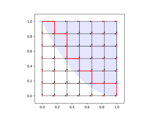
Figure 4: Visualization of the grid $G_{\varepsilon}$ for $\varepsilon=\nicefrac{{1}}{{6}}$. The shaded area represents the allocation region of some mechanism, while the red path is the corresponding inner hull.

5.1 The Discretization Lemma

We start by showing that against a $\sigma$-smooth adversary, it suffices to consider all mechanisms $\mathcal{M}_{\varepsilon}$ on the uniform $G_{\varepsilon}$ grid to obtain a small discretization error. This fact contrasts sharply with the case where we don’t impose smoothness; see Example 1. Given the smooth nature of the adversary, we can ignore what happens in regions of zero Lebesgue measure; therefore, we restrict our attention to complete paths in $G_{\varepsilon}$ that start from $(0,1)$ and terminate in $(1,0)$.

Lemma 2 (Discretization error for $\sigma$-smooth adversaries).

For any $\varepsilon>0$, any $\sigma\in(0,1]$, and any sequence of $\sigma$-smooth distributions, the following inequality holds:

$$\sup_{M\in\mathcal{M}}\sum_{t=1}^{T}\mathbb{E}\left[\textsf{rev}_{t}(M)\right]-\max_{M_{\varepsilon}\in\mathcal{M}_{\varepsilon}}\sum_{t=1}^{T}\mathbb{E}\left[\textsf{rev}_{t}(M_{\varepsilon})\right]\leq\frac{5}{\sigma}\varepsilon T.$$

Proof.

Fix $\varepsilon$, the sequence of $\sigma$-smooth distributions as in the statement, and consider any mechanism $\mathcal{M}^{\star}$ such that its total expected revenue is only at most an additive $\varepsilon T$ far from the one of the $\sup$. We define the inner-hull $H$ of $M^{\star}$ as the set of all the tiles in the grid $G_{\varepsilon}$ contained in the allocation region $A^{\star}$ of $M^{\star}$ (see Figure 4). Let $M$ be the mechanism in $\mathcal{M}_{\varepsilon}$ whose allocation region is the inner-hull $H$ of $M^{\star}$. For any time step $t$, we have the following inequality:

$$\mathbb{E}\left[\textsf{rev}_{t}(M^{\star})\right] =\mathbb{E}\left[\textsf{rev}_{t}(M^{\star})\mathbbm{1}_{\{{(v_{1}^{t},v_{2}^{t})\in H\}}}\right]+\mathbb{E}\left[\textsf{rev}_{t}(M^{\star})\mathbbm{1}_{\{{(v_{1}^{t},v_{2}^{t})\in A^{\star}\setminus H\}}}\right]$$

$$\leq\mathbb{E}\left[\textsf{rev}_{t}(M)\right]+2\mathbb{P}\left((v_{1}^{t},v_{2}^{t})\in A^{\star}\setminus H\right) \textsf{rev}_{t}(M^{\star})\leq 2$$ ()

$$\leq\mathbb{E}\left[\textsf{rev}_{t}(M)\right]+\tfrac{2}{\sigma}\nu(A^{\star}\setminus H)\leq\mathbb{E}\left[\textsf{rev}_{t}(M)\right]+4\tfrac{\varepsilon}{\sigma}. \sigma$$ (-smoothness)

Crucially, in the first inequality, we used that all the valuations in $H\subseteq A^{\star}$ result in trade under both mechanisms, but $M$ charges higher prices. Finally, the Lebesgue measure $\nu$ of $A^{\star}\setminus H$ is at most $2\varepsilon$ because it is contained in at most $\frac{2}{\varepsilon}$ tiles of $G_{\varepsilon}$ (all the tiles whose interior have a nonempty intersection with the boundary of $A^{\star}$) of area $\varepsilon^{2}$. ∎

5.2 Path Learning Algorithm

The discretization result in Lemma 2 and the bijection between the mechanisms $\mathcal{M}_{\varepsilon}$ and the set of all complete paths $\mathcal{P}_{\varepsilon}$ on $G_{\varepsilon}$, implies that it is enough for the learner to achieve sublinear regret with respect to the best mechanism in a large but finite class of candidates. We exploit this in our algorithm PathLearning, which is simply an instantiation of the well-known Hedge algorithm where each path in $\mathcal{P}_{\varepsilon}$ is an expert. We refer to the pseudocode for further details and to Section 5.3 for an efficient implementation of the sampling procedure. Before presenting the Theorem, which analyzes PathLearning, we observe that a simple combinatorial argument yields an upper bound on the number of mechanisms in $\mathcal{M}_{\varepsilon}$. The formal proof is deferred to Section A.3.

Lemma 3.

For any $\varepsilon>0$, the number $N_{\varepsilon}$ of mechanisms in $\mathcal{M}_{\varepsilon}$ is at most $2\cdot 4^{\nicefrac{{1}}{{\varepsilon}}}.$

Proof.

To show this, we consider the number of "down-right" paths in $G_{\varepsilon}$ from $(0,1)$ to $(1,0)$, as we know that there is a bijection between these paths and the mechanisms in $\mathcal{M}_{\varepsilon}$. Each path can be described by specifying which of its $\nicefrac{{2}}{{\varepsilon}}$ edges are the $\nicefrac{{1}}{{\varepsilon}}$ vertical edges and which are the $\nicefrac{{1}}{{\varepsilon}}$ horizontals. All in all:

$$N_{\varepsilon}=\binom{\nicefrac{{2}}{{\varepsilon}}}{\nicefrac{{1}}{{\varepsilon}}}\leq 2\cdot 4^{\nicefrac{{1}}{{\varepsilon}}},$$

where the inequality follows from Sterling’s inequalities (e.g., Formula 9.15 of Feller (1967)). ∎

We now have all the ingredients to prove the regret bound provided by PathLearning. We present a way to efficiently implement the algorithm in Section 5.3

Theorem 6.

Consider the Repeated Joint Ads problem against the $\sigma$-smooth adversary; then there exists a learning algorithm $\mathcal{A}$ such that

$$R_{T}(\mathcal{A})\leq\frac{13}{\sigma}\cdot T^{\nicefrac{{2}}{{3}}}.$$

Proof.

We prove that PathLearning with the right choice of the discretization and learning parameters verifies the statement of the Theorem. To this end, we combine Lemma 2 with the well-known regret bound of Hedge and optimize the two parameters:

$$R_{T}(\textsc{PathLearning}) =\sup_{M\in\mathcal{M}}\mathbb{E}\left[\sum_{t=1}^{T}\textsf{rev}_{t}(M)-\sum_{t=1}^{T}\textsf{rev}_{t}(M^{t})\right]$$

$$\leq\frac{5}{\sigma}\varepsilon T+\max_{M_{\varepsilon}\in\mathcal{M}_{\varepsilon}}\mathbb{E}\left[\sum_{t=1}^{T}\textsf{rev}_{t}(M_{\varepsilon})-\sum_{t=1}^{T}\textsf{rev}_{t}(M^{t})\right]$$

$$\leq\frac{5}{\sigma}\varepsilon T+4\sqrt{T\log N_{\varepsilon}}\leq\frac{5}{\sigma}\varepsilon T+8\sqrt{\frac{T}{\varepsilon}}\leq\frac{13}{\sigma}\cdot T^{\nicefrac{{2}}{{3}}},$$

where we used the standard bound of Hedge when the rewards are bounded in $[0,2]$ (see, e.g., Theorem 2.5 of Arora et al. (2012) for $\eta=T^{-\nicefrac{{1}}{{2}}}$), Lemma 3 and we set $\varepsilon=T^{-\nicefrac{{1}}{{3}}}$. ∎

1:Environment: Sequence of $\sigma$-smooth random variables $\{(V_{1}^{t},V_{2}^{t})\}$

2:Input: time horizon $T$, discretization parameter $\varepsilon\in(0,1)$ and learning parameter $\eta\in(0,1)$

3:For each path $\pi\in\mathcal{P}_{\varepsilon}$ set $w^{1}_{\pi}=1$ and $q^{1}_{\pi}=\frac{w^{1}_{\pi}}{W_{1}}$, where $W_{1}=\sum_{\pi\in\mathcal{P}_{\varepsilon}}w^{1}_{\pi}$.

4:for each round $t=1,2,\dots,T$ do

5:     Draw a path $\pi^{t}\in\mathcal{P}_{\varepsilon}$ according to the distribution $q^{t}$

6:     Implement the mechanism $M^{t}=M_{\pi^{t}}$ and observe $(v_{1}^{t},v_{2}^{t})\sim(V_{1}^{t},V_{2}^{t})$

7:     For each $\pi\in\mathcal{P}_{\varepsilon}$ set $w_{\pi}^{t}=w_{\pi}^{t}\cdot\exp{[\eta\cdot\textsf{rev}_{t}({M_{\pi}})]}$ and $q^{t}_{\pi}=\frac{w^{t}_{\pi}}{W_{t}}$, where $W_{t}=\sum_{\pi\in\mathcal{P}_{\varepsilon}}w^{t}_{\pi}$.

PathLearning

5.3 Sampling Efficiently: From Paths to Edges

We show how to efficiently implement the sampling step of PathLearning (line 5) without the need to maintain exponentially many weights (lines 3 and 7). We do this by constructing a sampling scheme that only maintains weights for the edges of $G_{\varepsilon}$, similarly to what is done, e.g., for online shortest path in Takimoto and Warmuth (2003) and György et al. (2005). The crucial idea is to maintain conditional-probability weights on the edges so that it is possible to sample paths from the desired distribution (line 5 of PathLearning) “one edge at a time” using these edge weights.

Theorem 7.

For any time step $t$ and sequence of valuations up to time $t$, excluded, there exist edge probabilities $q^{t}_{e}$ such that the following three properties hold:

• $q_{e}^{t}\in[0,1]$ for all $e$ edges in $G_{\varepsilon}$,

• $\sum_{e\in E_{u}^{+}}q_{e}^{t}=1$ for all node $u$ in $G_{\varepsilon}$, where $E_{u}^{+}$ are the outgoing edges from $u$

• $q_{\pi}^{t}=\prod_{e\in p}q^{t}_{e}$ for all paths $p\in\mathcal{P}_{\varepsilon}$.

Furthermore, it is possible to compute $q_{e}^{t}$ in time polynomial in $T$ and $\nicefrac{{1}}{{\varepsilon}}$.

Having access to the edge probabilities $q_{e}^{t}$, it is easy to sample from the distribution over paths as in line 5 of PathLearning by constructing the path one edge at the time, using the $q_{e}^{t}$ to pick the following edge.

Proof of Theorem 7.

We prove the Theorem in three steps. First, we define the edge version of the weights in lines 3 and 7 of PathLearning. For each edge $e$ in $G_{\varepsilon}$, let $A_{e}$ be the allocation rectangle it “covers” (this is the influence region defined for general orthogonal graphs in Definition 4): if $e$ is a vertical edge connecting $(\nicefrac{{i}}{{\varepsilon}},\nicefrac{{j}}{{\varepsilon}})$ to $(\nicefrac{{i}}{{\varepsilon}},\nicefrac{{j-1}}{{\varepsilon}})$, then $A_{e}$ is the rectangle $[\nicefrac{{i}}{{\varepsilon}},1]\times[\nicefrac{{j-1}}{{\varepsilon}},\nicefrac{{j}}{{\varepsilon}}]$, similarly, if $e$ is a horizontal edge connecting $(\nicefrac{{i}}{{\varepsilon}},\nicefrac{{j}}{{\varepsilon}})$ to $(\nicefrac{{i+1}}{{\varepsilon}},\nicefrac{{j}}{{\varepsilon}})$, then $A_{e}$ is the rectangle $[\nicefrac{{i}}{{\varepsilon}},\nicefrac{{i+1}}{{\varepsilon}}]\times[\nicefrac{{j}}{{\varepsilon}},1]$. Unlike in the general stochastic setting, the boundaries of the $A_{e}$ rectangles are irrelevant (as they carry no mass in smooth distributions). We can define the following edge weights:

$$w_{e}^{t}=\begin{cases}\exp{\{\eta\cdot\tfrac{i}{\varepsilon}\sum_{s=1}^{t-1}\mathbbm{1}_{\{{(v^{s}_{1},v^{s}_{2})\in A_{e}\}}}\}}\text{ if $e$ connects $(\tfrac{i}{\varepsilon},\tfrac{j}{\varepsilon})$ to $(\tfrac{i}{\varepsilon},\tfrac{j-1}{\varepsilon})$}\\ \exp{\{\eta\cdot\tfrac{j}{\varepsilon}\sum_{s=1}^{t-1}\mathbbm{1}_{\{{(v^{s}_{1},v^{s}_{2})\in A_{e}\}}}\}}\text{ if $e$ connects $(\tfrac{i}{\varepsilon},\tfrac{j}{\varepsilon})$ to $(\tfrac{i+1}{\varepsilon},\tfrac{j}{\varepsilon})$}\end{cases}$$

These weights are related to the ones used in Augment-the-Best-Mechanism but have a different meaning. We also highlight that it is possible to compute these weights efficiently. In particular, by exploiting the structure of the revenue function and the exponential nature of weights (both for paths and edges), we can derive a simple relationship between $w^{t}_{e}$ and the path-weights $w_{\pi}^{t}$ used by PathLearning. The formal proof is deferred to Section A.3.

Claim 3.

For any path $\pi\in\mathcal{P}_{\varepsilon}$ the following equality holds: $w_{\pi}^{t}=\prod_{e\in\pi}w_{e}^{t}$

Second, for every node $u=(\nicefrac{{i}}{{\varepsilon}},\nicefrac{{j}}{{\varepsilon}})$ of the graph $G_{\varepsilon}$ let $N^{+}_{u}$ be its out-neighborhood. We define $w_{(1,0)}^{t}=1$, and recursively the weights of the remaining nodes as follows: $w_{u}^{t}=\sum_{v\in N^{+}_{u}}w_{(u,v)}w_{v}^{t}.$

Note that the weights $w_{u}^{t}$ can be efficiently computed via dynamic programming starting from $w_{(1,0)}^{t}$. A node’s weight equals the sum of the weights of all the paths stemming from it. This property, formalized by the following claim whose proof is deferred to Section A.3, is crucial in defining the edge probabilities $q_{e}^{t}$.

Claim 4.

For any node $u\neq(1,0)$, let $\mathcal{P}^{u}_{\varepsilon}$ denote the $u$-$(1,0)$ paths, then $w_{u}^{t}=\sum_{\pi\in\mathcal{P}^{u}_{\varepsilon}}\prod_{e\in\pi}w^{t}_{e}$.

We are ready to define the edge probabilities $q_{e}^{t}$. Consider any node $u$; its outgoing edges have the following probabilities: if $N^{+}_{u}=\{v\}$, then $q_{(u,v)}^{t}=1$, else $N^{+}_{u}=\{d,r\}$ and the probabilities are

$$q_{(u,d)}^{t}=\tfrac{w_{(u,d)}^{t}\cdot w_{d}^{t}}{w_{(u,d)}^{t}\cdot w_{r}^{t}+w_{(u,r)}^{t}\cdot w_{r}^{t}}\text{ and }q_{(u,r)}^{t}=\tfrac{w_{(u,r)}^{t}\cdot w_{r}^{t}}{w_{(u,d)}^{t}\cdot w_{r}^{t}+w_{(u,r)}^{t}\cdot w_{r}^{t}}.$$

Now, properties (i) and (ii) in Theorem 7 are clearly respected by $q_{e}^{t}$; we need to make sure that also the last property holds. For any $\pi=(e_{1},e_{2},\dots,e_{k})$, it holds that

$$\mathbb{P}\left(\pi^{t}=\pi\right)=\prod_{i=1}^{k}\mathbb{P}\left((e_{1},e_{2},\dots,e_{i})\in\pi^{t}\mid(e_{1},e_{2},\dots,e_{i-1})\in\pi^{t}\right).$$

It then suffices to show that for any path $\pi$ and any $i=1,\dots,k$ the following equality holds

$$\mathbb{P}\left((e_{1},e_{2},\dots,e_{i})\in\pi^{t}\mid(e_{1},e_{2},\dots,e_{i-1})\in\pi^{t}\right)=q_{e_{i}}^{t}.$$ (3)

Equation 3 follows by a simple case analysis which is deferred to 7 in Section A.3. ∎

6 A $\sqrt{T}$ Lower Bound for the Smooth and the Stochastic Adversaries

We construct a hard instance for the Repeated Joint Ads Problem, which forces any learner to suffer at least $\Omega(\sqrt{T})$ regret. Such instance is based on a smooth distribution from which valuations are drawn i.i.d., thus yielding a lower bound for both the smooth and the stochastic i.i.d. setting.

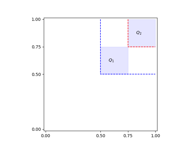
Figure 5: The two squares support the family of distributions we use in the lower bound. In blue, respectively red, are reported the boundary of the allocation region of $M_{1}$, respectively $M_{2}$.

We introduce a family of smooth distributions, parameterized by $\alpha\in(\nicefrac{{4}}{{15}},\nicefrac{{2}}{{5}})$. For the sake of simplicity, we denote with $V=(V_{1},V_{2})$ the random variables describing the agents’ valuations, and with $\mathbb{P}^{\alpha}$ the probability measure (and with $\mathbb{E}^{\alpha}$ the expectation) under which $V$ has the following density:

$$f_{\alpha}(v_{1},v_{2})=16\left(\alpha\mathbbm{1}_{\{{(v_{1},v_{2})\in Q_{1}\}}}+(1-\alpha)\mathbbm{1}_{\{{(v_{1},v_{2})\in Q_{2}\}}}\right),$$

where $Q_{1}=[\nicefrac{{1}}{{2}},\nicefrac{{3}}{{4}}]\times[\nicefrac{{1}}{{2}},\nicefrac{{3}}{{4}}]$ and $Q_{2}=[\nicefrac{{3}}{{4}},1]\times[\nicefrac{{3}}{{4}},1]$ (see also Figure 5). In other words, under $\mathbb{P}^{\alpha}$ the random variable $V$ is drawn from a mixture of two uniform distributions, one supported on $Q_{1}$ (with probability $\alpha$) and one on $Q_{2}$ (with the remaining probability $1-\alpha$). A simple calculation shows the smoothness of the family, in particular, for any $\alpha\in(\nicefrac{{4}}{{15}},\nicefrac{{2}}{{5}})$, $\mathbb{P}^{\alpha}$ is $\nicefrac{{1}}{{12}}$-smooth. We introduce two mechanisms:

• Mechanism $M_{1}$, which allocates in the $[\nicefrac{{1}}{{2}},1]\times[\nicefrac{{1}}{{2}},1]$ square with $\mathbb{E}^{\alpha}\left[\textsf{rev}(M_{1})\right]=1$

• Mechanism $M_{2}$, which allocates in the $[\nicefrac{{3}}{{4}},1]\times[\nicefrac{{3}}{{4}},1]$ square with $\mathbb{E}^{\alpha}\left[\textsf{rev}(M_{2})\right]=\tfrac{3}{2}(1-\alpha)$.

Specifically, it is possible to prove that for any $\mathbb{P}^{\alpha}$, either $M_{1}$ or $M_{2}$ are optimal, as they always dominate the other mechanisms. We present the formal result in the following Lemma, whose proof (as the complete one of the main Theorem) is deferred to Section A.4.

Lemma 4 (Domination).

Fix any $\alpha\in(\nicefrac{{4}}{{15}},\nicefrac{{2}}{{5}})$ and any mechanism $M$, and let $A_{M}$ be its allocation region. Then, the following properties hold

• If $A_{M}\cap Q_{1}\neq\emptyset$, then $\mathbb{E}^{\alpha}\left[\textsf{rev}(M_{1})\right]\geq\mathbb{E}^{\alpha}\left[\textsf{rev}(M)\right]$.

• If $A_{M}\cap Q_{1}=\emptyset$, then $\mathbb{E}^{\alpha}\left[\textsf{rev}(M_{2})\right]\geq\mathbb{E}^{\alpha}\left[\textsf{rev}(M)\right]$.

Theorem 8.

Consider the Repeated Joint Ads problem against the $\sigma$-smooth adversary, for $\sigma\in(0,\nicefrac{{1}}{{12}})$, then any learning algorithm $\mathcal{A}$ suffers regret $R_{T}(\mathcal{A})\geq\tfrac{3}{64}\sqrt{T}.$

Proof Sketch.

Let $\varepsilon$ be a small parameter to be set later, and let $\alpha_{0}=\nicefrac{{1}}{{3}}$. We consider two probability distributions from the family introduced above, corresponding to parameters $\alpha_{0}+\varepsilon$ and $\alpha_{0}-\varepsilon$. Consider an adversary that selects one of these two distributions uniformly at random and extracts the valuations i.i.d. from it. We sketch here an explanation of why any learning algorithm suffers regret $\Omega(\sqrt{T})$ against this adversary, and defer the formal proof to Section A.4. Lemma 4 critically tells us that we can restrict our attention, without loss of generality, to learning algorithms that only play the two mechanisms $M_{1}$ and $M_{2}$ described above. $M_{1}$ is optimal for the first distribution, while $M_{2}$ is optimal on the second. Moreover, their revenue is an additive $\Theta(\varepsilon)$ away from each other, so that posting the wrong mechanism incurs an instantaneous regret of $\Theta(\varepsilon)$. Any learning algorithm needs $\Omega(\nicefrac{{1}}{{\varepsilon^{2}}})$ samples to establish which one of the two instances it is playing against and suffers loss $\Theta(\varepsilon)$ until it discovers it. If $\varepsilon$ is too small, the learner cannot discover the best mechanism with high probability, thus suffering a regret of $\Omega(\varepsilon T)$. All in all, it suffers $\Omega(\min\{\nicefrac{{1}}{{\varepsilon}},\varepsilon T\})$ regret. Setting $\varepsilon=\nicefrac{{1}}{{\sqrt{T}}}$ yields the desired result. ∎

Corollary 1.

Any learning algorithm suffers $\Omega(\sqrt{T})$ regret in the stochastic i.i.d. setting.

7 Conclusion

Motivated by online retail, in this paper, we introduced the online version of the Joint Ads Problem, in which two buyers (e.g., a merchant and a brand) cooperate to secure a non-excludable good (e.g., an ad slot). This problem is similarly fundamental to non-excludable mechanism design, as the single-buyer single-item problem is to excludable mechanism design. We have studied the problem in various data-generation models, providing efficient learning algorithms for the stochastic and the $\sigma$-smooth framework. We complemented these positive results with various lower bounds, in particular proving that in the adversarial setting, it is impossible to achieve sublinear regret. Many interesting questions remain, including settling the minimax regret in the stochastic and $\sigma$-smooth models. Additionally, it would be interesting to see if our adaptive discretization technique can be useful for other related problems. Finally, we hope our work can be a stepping stone for future investigation that extends our results to more buyers (bigger groups and multiple groups).

Appendix A Supplementary Material

A.1 The Learning complexity of $\mathcal{M}$ and $\mathcal{M}^{\perp}$

We prove that for any $\varepsilon\in(0,1)$, the pseudo-dimension of $\mathcal{M}_{\varepsilon}\subseteq\mathcal{M}^{\perp}$ is $\Omega(\nicefrac{{1}}{{\varepsilon}})$. This result implies that the class of all mechanisms has unbounded pseudo-dimension and that the same holds for $\mathcal{M}^{\perp}$. We start by recalling the definition of pseudo-dimension of a class of functions. Let $\mathcal{Q}$ be a set and consider a class $\mathcal{F}$ of functions $f:\mathcal{Q}\to[0,H]$. Let $S$ be $m$ points in $\mathcal{Q}$, labeled according to $f$, meaning that for each sample $x\in S$, $f(x)$ is known for all $f\in\mathcal{F}$. Let $(r_{1},r_{2},\dots,r_{m})\in[0,H]^{m}$ be a set of targets for $S$. We say that $(r_{1},r_{2},\dots,r_{m})$ witnesses the shattering of $S$ by $\mathcal{F}$ if, for each $T\subseteq S$, there exists some $f_{T}\in\mathcal{F}$ such that $f_{T}(x_{i})\geq r_{i}$ for all $x_{i}\in T$ and $f_{T}(x_{i})<r_{i}$ for all $x_{i}\in S\setminus T$. If there exists some $(r_{1},r_{2},\dots,r_{m})$ witnessing the shattering of $S$, we say that $S$ is shatterable by $\mathcal{F}$.

Definition 7.

The pseudo-dimension of $\mathcal{F}$ is the size of the largest set $S$ shatterable by $\mathcal{F}$.

In our setting, the set $\mathcal{Q}$ is $[0,1]^{2}$, $H=2$ and $\mathcal{F}$ is the set of all functions $f=f_{M}$ which map valuations to revenue according to some mechanism $M\in\mathcal{M}.$ For simplicity, we refer to the pseudo-dimension of $\mathcal{M}$ (or some subset of $\mathcal{M}$) without specifying that we are actually studying the complexity of the class of functions just described.

Theorem 9.

For any $\varepsilon\in(0,1)$, such that $\nicefrac{{1}}{{\varepsilon}}\in\mathbb{N}$, the pseudo-dimension of $M_{\varepsilon}$ is $\Omega(\nicefrac{{1}}{{\varepsilon}})$.

Proof.

Consider $S=\{(i\varepsilon,1-i\varepsilon)\in[0,1]^{2}\mid i=1,2,\dots\nicefrac{{1}}{{\varepsilon}}\}$, we show that these $\nicefrac{{1}}{{\varepsilon}}$ points are shattered by $\mathcal{M}_{\varepsilon}$, using the vector $(1,1,\dots,1)\in[0,2]^{\nicefrac{{1}}{{\varepsilon}}}$ has witness. For any subset $T$ of these points, it is easy to find a path on $G_{\varepsilon}$ which passes through all the nodes in $T$ (thus ensuring a revenue of $1$ and clearing the witness condition on these points), and whose allocation region does not contain the vertices in $S\setminus T$ (thus getting no revenue from them and clearing the witness condition on these points). We refer to Figure 6 for a visualization. ∎

We have two immediate corollaries.

Corollary 2.

The pseudo-dimension of $\mathcal{M}^{\perp}$ and $\mathcal{M}$ is unbounded.

Corollary 3.

The VC dimension of all the monotone regions is unbounded.

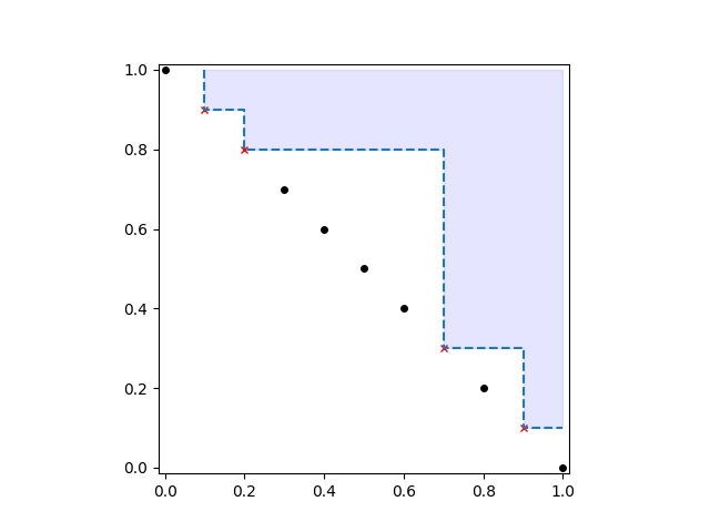
Figure 6: Example of the mechanism shattering points on the diagonal. The red points correspond to $T$ and yield revenue $1$ in the mechanisms corresponding to the shaded allocation region. All the black points in $S\setminus T$ are not in the allocation region and thus generate $0$ revenue.

A.2 Proofs Omitted from Section 4

See 3

Proof.

We start by deriving closed-form solutions for $a_{t}$ and $b_{t}$, parameterized by the sets $L$ and $R$, which correspond to the coin tosses that lead to the two cases in constructing the input sequence. That is, $t\in R$ with probability $\zeta$ (i.e., $(v_{1}^{t},v_{2}^{t})=(b_{t},1)$) and $t\in L$ with probability $1-\zeta$ (i.e., $(v_{1}^{t},v_{2}^{t})=(a_{t},\zeta)$). We say that $t=0$ belongs to $R$ for convenience. Define

$$\alpha_{t}=\begin{cases}2&\text{if $t\in R$}\\ 1&\text{if $t\in L$}\\ \end{cases}\quad\text{and}\quad\gamma_{t}=\begin{cases}+1&\text{if ${t-1}\in R$}\\ -1&\text{if $t-1\in L$}\end{cases}.$$

Claim 5.

For any realization of the coin tosses, we have the following closed-form

$$a_{t}=\gamma_{t}\cdot\Delta_{t}+\sum_{j=1}^{t-1}\gamma_{j}\cdot\alpha_{j}\cdot\Delta_{j}\quad\text{and}\quad b_{t}=2\cdot\gamma_{t}\cdot\Delta_{t}+\sum_{j=1}^{t-1}\gamma_{j}\cdot\alpha_{j}\cdot\Delta_{j}.$$

Proof of 5.

We prove the claim by induction. For $t=1$ we have

$$a_{1}=\gamma_{1}\cdot\Delta_{1}=\Delta_{1}=\tfrac{\delta}{3}\quad\text{and}\quad b_{1}=2\cdot\gamma_{1}\cdot\Delta_{1}=2\cdot\Delta_{1}=\tfrac{2\delta}{3},$$

as needed. For the inductive step, assume the claim is true up to $t$. We distinguish the two cases according to whether $t\in R$ or $L$. If $t\in R$. Then, by the induction hypothesis, we have:

$$a_{t+1} =b_{t}+\Delta_{t+1}=\left[\left(\sum_{j=1}^{t-1}\gamma_{j}\cdot\alpha_{j}\cdot\Delta_{j}\right)+\gamma_{t}\cdot 2\cdot\Delta_{t}\right]+\Delta_{t+1}$$

$$=\left[\left(\sum_{j=1}^{t-1}\gamma_{j}\cdot\alpha_{j}\cdot\Delta_{j}\right)+\gamma_{t}\cdot\alpha_{t}\cdot\Delta_{t}\right]+\gamma_{t+1}\cdot\Delta_{t+1}=\left(\sum_{j=1}^{t}\gamma_{j}\cdot\alpha_{j}\cdot\Delta_{j}\right)+\gamma_{t+1}\cdot\Delta_{t+1}$$

and similarly

$$b_{t+1} =b_{t}+2\cdot\Delta_{t+1}=\left[\left(\sum_{j=1}^{t-1}\gamma_{j}\cdot\alpha_{j}\cdot\Delta_{j}\right)+\gamma_{t}\cdot 2\cdot\Delta_{t}\right]+2\cdot\Delta_{t+1}$$

$$=\left[\left(\sum_{j=1}^{t-1}\gamma_{j}\cdot\alpha_{j}\cdot\Delta_{j}\right)+\gamma_{t}\cdot\alpha_{t}\cdot\Delta_{t}\right]+\gamma_{t+1}\cdot 2\cdot\Delta_{t+1}=\left(\sum_{j=1}^{t}\gamma_{j}\cdot\alpha_{j}\cdot\Delta_{j}\right)+\gamma_{t+1}\cdot 2\cdot\Delta_{t+1}.$$

The remaining case, i.e., when $t\in L$ is analogous. ∎

The closed formulas in Claim 5 are all we need to prove point (i) of the Proposition: for all $t$:

$$a_{t}=\left(\sum_{j=1}^{t-1}\gamma_{j}\cdot\alpha_{j}\cdot\Delta_{j}\right)+\gamma_{t}\cdot\Delta_{t}\leq\sum_{j=1}^{T}2\cdot\Delta_{j}\leq 2\sum_{j=1}^{\infty}\frac{\delta}{3^{j}}=\delta.$$

On the other hand, we have that

$$a_{t}=\left(\sum_{j=1}^{t-1}\gamma_{j}\cdot\alpha_{j}\cdot\Delta_{j}\right)+\gamma_{t}\cdot\Delta_{t}\geq\Delta_{1}-\sum_{j=2}^{\infty}2\cdot\Delta_{j}=\frac{\delta}{3}-2\left(\bigg{(}\sum_{j=1}^{\infty}\frac{\delta}{3^{j}}\bigg{)}-\frac{\delta}{3}\right)=0.$$

Similarly, again by Claim 5, for all $t$, it is possible to verify that $b_{t}\in(0,\delta)$. We omit the calculations that are analogous. as claimed. To address point (ii) of the Proposition, we exploit a natural notion of monotonicity. Formally, we have the following result.

Claim 6.

The sequence $a_{t}$ is decreasing for $t\in R$, while $b_{t}$ is increasing for $t\in L$.

Proof of 6.

We prove the result for $t\in R$; the other case is analogous. Fix any $t$ and $t^{\prime}$ with $t<t^{\prime}$ both in $R$, such that no intermediate time step is in $R$, we have the following:

$$b_{t^{\prime}}-b_{t}=2\Delta_{t+1}-\left(\sum_{j=t+2}^{t^{\prime}}2\Delta_{j+1}\right)=2\delta\left(\frac{1}{3^{t+1}}-\sum_{j=t+2}^{t^{\prime}}\frac{1}{3^{j}}\right)\geq\frac{2\delta}{3^{t+1}}\left(1-\sum_{j=1}^{\infty}\frac{1}{3^{j}}\right)=\frac{\delta}{3^{t+1}}>0.\qed$$

To show that there exists a threshold $\tau\in(0,1)$ that separates the two sequences, it suffices to show that for $t^{\prime},t^{\prime\prime}$ such that $t^{\prime}$ is the last index in $L$, and $t^{\prime\prime}$ is the last one in $R$, it holds that $b_{t^{\prime\prime}}<a_{t^{\prime}}$. This property is sufficient because then we can choose $\tau$ halfway between $b_{t^{\prime\prime}}$ and $a_{t^{\prime}}$ to ensure that $\tau\in(0,\delta)$ (by point (i) of the Proposition), while for all $(a_{t},\zeta)$ resp. $(b_{t},1)$ in the sequence it will hold that $a_{t}\geq a_{t^{\prime\prime}}>\tau$ resp. $b_{t}<b_{t^{\prime\prime}}<\tau$ (by Claim 6).

Case 1:

$t^{\prime}<t^{\prime\prime}$. In this case, by the definition of $t^{\prime}$ and $t^{\prime\prime}$, we have that

$$b_{t^{\prime\prime}} =a_{t^{\prime}}-2\Delta_{t+1}+\sum_{j=t+2}^{T}2\Delta_{j}=a_{t^{\prime}}-2\frac{\delta}{3^{t+1}}+\sum_{j=t+2}^{T}2\frac{\delta}{3^{j}}$$

$$<a_{t^{\prime}}-2\frac{\delta}{3^{t+1}}+\sum_{j=t+2}^{\infty}2\frac{\delta}{3^{j}}=a_{t^{\prime}}-2\frac{\delta}{3^{t+1}}\left(1-\sum_{j=1}^{\infty}\frac{1}{3^{j}}\right)=a_{t^{\prime}}-\frac{\delta}{3^{t+1}}<a_{t^{\prime}}.$$

Case 2:

$t^{\prime}>t^{\prime\prime}$. In this case, we can again use the definition of $t^{\prime}$ and $t^{\prime\prime}$ to conclude that

$$a_{t^{\prime}} =b_{t^{\prime\prime}}+\Delta_{t+1}-\sum_{j=t+2}^{T}\Delta_{j}=b_{t^{\prime}}+\frac{\delta}{3^{t+1}}-\sum_{j=t+2}^{T}\frac{\delta}{3^{j}}$$

$$>b_{t^{\prime\prime}}+\frac{\delta}{3^{t+1}}-\sum_{j=t+2}^{\infty}\frac{\delta}{3^{j}}=b_{t^{\prime\prime}}+\frac{\delta}{3^{t+1}}\left(1-\sum_{j=1}^{\infty}\frac{1}{3^{j}}\right)=b_{t^{\prime\prime}}+\frac{\delta}{2\cdot 3^{t+1}}>b_{t^{\prime\prime}}.\qed$$

A.3 Proofs Omitted from Section 5

See 3

Proof of 3.

Fix any sequence of valuations $(v_{1}^{1},v_{2}^{1}),\dots(v_{1}^{t},v_{2}^{t})$ and any path $\pi\in\mathcal{P}_{\varepsilon}$ (with $M=M_{\pi}$ as its associated mechanism), we prove the following equality, which implies the statement of the claim:

$$\sum_{s=1}^{t}\textsf{rev}_{s}(M)=\sum_{s=1}^{t}\sum_{e\in\pi}w_{e}\mathbbm{1}_{\{{(v^{s}_{1},v^{s}_{2})\in A_{e}\}}},$$

where $w_{e}$ is the intrinsic weight defined in Definition 4 and stands for $\nicefrac{{i}}{{\varepsilon}}$ if $e$ connects $(\nicefrac{{i}}{{\varepsilon}},\nicefrac{{j}}{{\varepsilon}})$ to $(\nicefrac{{i}}{{\varepsilon}},\nicefrac{{j-1}}{{\varepsilon}})$ or $(\nicefrac{{j}}{{\varepsilon}},\nicefrac{{i}}{{\varepsilon}})$ to $(\nicefrac{{j+1}}{{\varepsilon}},\nicefrac{{i}}{{\varepsilon}})$. In particular, it is enough to prove that, for any time step $s$, the following hold:

$$\textsf{rev}_{s}(M)=\sum_{e\in p}w_{e}\mathbbm{1}_{\{{(v^{s}_{1},v^{s}_{2})\in A_{e}\}}}.$$ (4)

To see why this equality holds, we consider two cases, according to whether a trade happened or not. If $(v_{1}^{s},v_{2}^{s})$ does not lie in the allocation region of $M$, then it means there is no rectangle $A_{e}$ with $e\in\pi$ that contains it: therefore, the two sides of Equation 4 are both $0.$ If $(v_{1}^{s},v_{2}^{s})$ induces a trade, then it belongs to precisely two rectangles $A_{e}$ and $A_{e^{\prime}}$ for $e,e^{\prime}$ (with $e$ horizontal and $e^{\prime}$ vertical, note this holds because the realized valuations belong to the edges of $G_{\varepsilon}$ with zero probability) in $\pi$; in particular, the payments of the agents for the mechanisms are exactly $w_{e}$ (for the second agents) and $w_{e^{\prime}}$ (for the first agent). ∎

See 4

Proof of 4.

We prove this result by induction on the distance $d$ of $u$ to the sink $(1,0)$. We start with the base case $d=1$ for which the equality clearly holds: there are only two nodes to consider there, $(1-\nicefrac{{1}}{{\varepsilon}},0)$ and $(1,\nicefrac{{1}}{{\varepsilon}})$ and only one edge connecting them to $(1,0)$ (recall the weight of the node $(1,0)$ is set to $1$).

We now consider the general case and let $N_{u}^{+}$ be its out-neighborhood and $E_{u}^{+}$ the edge(s) that connect(s) $u$ to its neighbor(s). The paths in $\mathcal{P}_{\varepsilon}^{u}$ can be divided according to their first edge:

$$w_{u}^{t} =\sum_{v\in N_{u}^{+}}w_{(u,v)}w_{v}^{t}=\sum_{v\in N_{u}^{+}}w_{(u,v)}\sum_{\pi^{\prime}\in\mathcal{P}_{\varepsilon}^{v}}\prod_{e\in\pi^{\prime}}w_{e}^{t}=\sum_{\pi\in\mathcal{P}_{\varepsilon}^{u}}\prod_{e\in\pi}w_{e}^{t},$$ (5)

where the first equality is due to the $w_{u}^{t}$ definition, and the second to the induction hypothesis. ∎

Claim 7.

It holds that $\mathbb{P}\left((e_{1},e_{2},\dots,e_{i})\in\pi^{t}\mid(e_{1},e_{2},\dots,e_{i-1})\in\pi^{t}\right)=q_{e_{i}}^{t}.$

Proof.

We have two cases: if $e_{i}$ is the only possible edge after $e_{i-1}$, i.e., the endpoint of $e_{i-1}$ has only one out-neighbor, then Equation 3 holds as both the sides of the formula are $1.$ Consider now the other case. Let $u$ be the end-point of edge $e_{i-1}$, $d$ and $r$ the two out-neighbors of $u$ and assume without loss of generality that $e_{i}=(u,r)$. To simplify notation, let $\mathcal{P}_{:i}$ be the set of all paths that coincide with $(e_{1},\dots,e_{k})$ up to its $i^{th}$ edge, included. We have the following chain of equalities:

$$\mathbb{P}((e_{1},e_{2},\dots,e_{i})\in\pi^{t}\mid(e_{1},e_{2},\dots,e_{i-1})\in\pi^{t}) =\frac{\mathbb{P}\left((e_{1},e_{2},\dots,e_{i})\in\pi^{t}\right)}{\mathbb{P}\left((e_{1},e_{2},\dots,e_{i-1})\in\pi^{t}\right)}$$

$$=\frac{\sum_{\pi\in\mathcal{P}_{:i}}q^{t}_{\pi}}{\sum_{\pi^{\prime}\in\mathcal{P}_{:i-1}}q^{t}_{\pi^{\prime}}}=\frac{\sum_{\pi\in\mathcal{P}_{:i}}w^{t}_{\pi}}{\sum_{\pi^{\prime}\in\mathcal{P}_{:i-1}}w^{t}_{\pi^{\prime}}},$$

where we exploited the definition of the $q_{\pi}^{t}$. We apply 3 on the right-most term of the previous formula to express the path weights in terms of the edge weights. To simplify notation, for any fixed path $\pi$, we denote with $\pi_{:i}$ its prefix of the first $i$ edges (included). We get:

$$\mathbb{P}((e_{1},e_{2},\dots,e_{i})\in\pi^{t} \mid(e_{1},e_{2},\dots,e_{i-1})\in\pi^{t})=\frac{\sum_{\pi\in\mathcal{P}_{:i}}w^{t}_{\pi}}{\sum_{\pi^{\prime}\in\mathcal{P}_{:i-1}}w^{t}_{\pi^{\prime}}}$$

$$=\frac{\sum_{\pi\in\mathcal{P}_{:i}}\prod_{e\in\pi}w_{e}^{t}}{\sum_{\pi^{\prime}\in\mathcal{P}_{:i-1}}\prod_{e^{\prime}\in\pi^{\prime}}w_{e^{\prime}}^{t}}$$

$$=\frac{w_{e_{i}}^{t}\sum_{p\in\mathcal{P}_{:i}}\prod_{e\in p_{:i-1}}w_{e}^{t}}{w_{e_{i}}^{t}\sum_{p\in\mathcal{P}_{:i}}\prod_{e\in p_{:i-1}}w_{e}^{t}+w_{(u,d)}^{t}\sum_{p\in\mathcal{P}_{:i}}\prod_{e\in p_{:i-1}}w_{e}^{t}}$$

$$=\frac{w_{e_{i}}^{t}w_{u}^{t}}{w_{e_{i}}^{t}w_{u}^{t}+w_{(u,d)}^{t}w_{d}^{t}}=q_{e}^{t},$$

where the second to last equality follows by 4 and the last one by definition of $q_{e}^{t}.$ ∎

A.4 Proofs Omitted from Section 6

Before providing the formal proofs that we omitted from Section 6, we recall some results from the literature on the “one-shot” version of the problem. We recall the definition of virtual valuation, crucial in characterizing revenue-maximizing auctions [Myerson, 1981, Güth and Hellwig, 1986].

Definition 8.

(Virtual Valuation) Let $X$ be a random variable with probability density function $f_{X}:[a,b]\to\mathbb{R}_{+}$ and cumulative density function $F_{X}$. If $f_{X}$ is strictly positive on its domain, we can define the virtual valuation function $\phi_{X}:[a,b]\to\mathbb{R}$ as follows:

$$\phi_{X}(x)=x-\frac{1-F(x)}{f(x)}.$$

The random variable $X$ is regular if $\phi_{X}$ is monotone non-decreasing on its domain.

Example 2.

The virtual valuations of a uniform random variable $U$ in $[a,b]$ is $\phi_{U}(x)=2x-b.$

We present a simple lemma that is crucial to the following construction.

Lemma 5.

Consider agents whose valuations are drawn from a uniform distribution on a rectangle $R=[a,b]\times[c,d]$. The following properties hold:

• For any mechanism $M$ with allocation region $A_{M}$, it holds that

  $$\mathbb{E}\left[\textsf{rev}(M)\right]=\frac{1}{(b-a)(d-c)}\int_{A_{M}\cap R}(2(v_{1}+v_{2})-(b+d))dv_{1}dv_{2}$$

• The optimal mechanism $M^{\star}$ allocates if and only if $2(v_{1}+v_{2})\geq(b+d)$.

• If $2(a+c)\geq b+d$, then the optimal mechanism always allocates, with $\mathbb{E}\left[\textsf{rev}(M^{\star})\right]=a+c$

Proof.

Denote with $V_{1}$ and $V_{2}$ the two independent uniform random variables that represent the two valuations. When the valuations of the two agents are drawn by two independent and regular distributions $V_{1}$ and $V_{2}$, then the expected revenue is equal to the expected virtual surplus (e.g., Theorem 13.10 of Nisan et al. [2007]), this proves point (i). The optimal mechanism then allocates if and only if the sum of the virtual valuations is positive, i.e., if the realized $v_{1}$ and $v_{2}$ are such that

$$\phi_{V_{1}}(v_{1})+\phi_{V_{2}}(v_{2})=2(v_{1}+v_{2})-(b+d)\geq 0.$$ (6)

Stated differently, the optimal mechanism allocates if and only if $2(v_{1}+v_{2})\geq(b+d)$. This proves point (ii). Finally, the expected revenue is then easy to compute when $2(v_{1}+v_{2})\geq 2(a+c)\geq(b+d)$, i.e., when the trade always happens: with probability $1$, the first agent pays $a$, and the second $c$. Equivalently, This can be computed by integrating the virtual valuation on the allocation region:

$$\mathbb{E}\left[\textsf{rev}(M^{\star})\right]=\frac{1}{(b-a)(d-c)}\int_{a}^{b}\int_{c}^{d}[2(v_{1}+v_{2})-(b+d)]dv_{2}dv_{1}=a+c.$$

This shows (iii) and completes the proof. ∎

See 4

Proof.

Let $M$ be any mechanism and $\alpha$ any parameter in $(\nicefrac{{4}}{{15}},\nicefrac{{3}}{{5}})$. We prove the Lemma via a case analysis, according to the relative position of its allocation region $A_{M}$ and the support of $\mathbb{P}^{\alpha}$.

Case I

If $Q_{1}\cup Q_{2}\subseteq A_{M}$, $M$ always trades the item, and $M_{1}$ clearly dominates $M$ (by monotonicity, the highest price any valuation in $A_{M}$ can be charged is $\nicefrac{{1}}{{2}}$ for each agent, which is what $M_{1}$ does).

Case II

If $Q_{1}\cap A_{M}=\emptyset$, then $M$ only considers valuations in $Q_{2}$, but we know that the optimal mechanism that considers only $Q_{2}$ is $M_{2}$ (by Lemma 5).

The first two cases rule out all the mechanisms such that the intersection of $A_{M}$ and $Q_{1}$ is not proper ($A_{M}\cap Q_{1}=Q_{1}$ in the first case and $A_{M}\cap Q_{1}=\emptyset$ in the second). Moreover, if $A_{M}\cap Q_{1}\neq\emptyset$, then $Q_{2}\subseteq A_{M}$, by monotonicity of the allocation rule (for any $(x_{1},y_{1})$ in $Q_{1}$ and $(x_{2},y_{2})$ in $Q_{2}$ it holds that $x_{1}\leq x_{2}$ and $y_{1}\leq y_{2}$). For the sake of simplicity, we denote with $\ell_{i}$ the sides of $Q_{1}$, naming $\ell_{1}$ the $(\nicefrac{{1}}{{2}},\nicefrac{{3}}{{4}})$-$(\nicefrac{{3}}{{4}},\nicefrac{{3}}{{4}})$ segment and proceeding clock-wise.

Case III

The boundary of $A_{M}$ intersects $\ell_{1}$ in $(x,\nicefrac{{3}}{{4}})$ and $\ell_{3}$ in $(y,\nicefrac{{1}}{{2}})$, with $\nicefrac{{1}}{{2}}\leq x\leq y\leq\nicefrac{{3}}{{4}}.$ Then, without loss of generality, we can assume that $M$ is completed by the segments $(x,\nicefrac{{3}}{{4}})-(x,1)$ and $(y,\nicefrac{{1}}{{2}})-(1,\nicefrac{{1}}{{2}})$. So the behaviour of $M$ with respect to the valuations in $Q_{2}$ is fixed: accept them and charge $x+\nicefrac{{1}}{{2}}$. The behavior of $M$ inside $Q_{1}$ is not clear. However, the virtual valuation is positive on $Q_{1}$; thus, by Lemma 5, the best thing $A_{M}\cap Q_{1}$ can be is the whole $[x,\nicefrac{{3}}{{4}}]\times[\nicefrac{{1}}{{2}},\nicefrac{{3}}{{4}}]$ rectangle, with an expected revenue of $(x+\tfrac{1}{2})$ times the probability of a trade. We thus have

$$\mathbb{E}\left[\textsf{rev}{(M)}\right] \leq(x+\tfrac{1}{2})[(1-\alpha)+\alpha({3-4x})]$$

$$\leq\max_{x\in[\nicefrac{{1}}{{2}},\nicefrac{{3}}{{4}}]}(x+\tfrac{1}{2})[(1-\alpha)+\alpha({3-4x})]=1=\mathbb{E}\left[\textsf{rev}(M_{1})\right],$$

where we used that the $\max$ is attained in $x=\nicefrac{{1}}{{2}}$ for all relevant $\alpha$.

Case IV

The boundary of $A_{M}$ intersects $\ell_{1}$ in $(x,\nicefrac{{3}}{{4}})$ and $\ell_{2}$ in $(\nicefrac{{3}}{{4}},y)$, with $\nicefrac{{1}}{{2}}\leq x,y\leq\nicefrac{{3}}{{4}}.$ Reasoning as in Case III, the best possibility for $M$ is that $A_{M}\cap M_{1}=[x,\nicefrac{{3}}{{4}}]\times[y,\nicefrac{{3}}{{4}}]$, for an expected revenue of $(x+y)$ times the probability of a trade. We thus have:

$$\mathbb{E}\left[\textsf{rev}{(M)}\right] \leq(x+y)[(1-\alpha)+\alpha({3-4x})(3-4y)]$$

$$\leq(x+\tfrac{1}{2})[(1-\alpha)+\alpha({3-4x})]$$

$$\leq\max_{x\in[\nicefrac{{1}}{{2}},\nicefrac{{3}}{{4}}]}(x+\tfrac{1}{2})[(1-\alpha)+\alpha({3-4x})]=1=\mathbb{E}\left[\textsf{rev}(M_{1})\right],$$

where the second inequality can be verified to hold numerically for any choice of the parameter $\alpha\in(\nicefrac{{4}}{{15}},\nicefrac{{2}}{{5}})$, and of $x$ and $y$ in $[\nicefrac{{1}}{{2}},\nicefrac{{3}}{{4}}]$.

Case IV

The boundary of $A_{M}$ intersects $\ell_{4}$ in $(\nicefrac{{1}}{{2}},x)$ and $\ell_{3}$ in $(y,\nicefrac{{1}}{{2}})$, with $\nicefrac{{1}}{{2}}\leq y,x\leq\nicefrac{{3}}{{4}}.$ This case is easy: by using Lemma 5 and reasoning as in Case III the best possibility for $A_{M}$ is to contain the whole $Q_{1}$ (which is exactly what $M_{1}$ does).

Case V

The boundary of $A_{M}$ intersects $\ell_{4}$ in $(\nicefrac{{1}}{{2}},x)$ and $\ell_{2}$ in $(\nicefrac{{3}}{{4}},y)$, with $\nicefrac{{1}}{{2}}\leq y\leq x\leq\nicefrac{{3}}{{4}}.$ This case is analogous to Case IV (by symmetry). ∎

See 8

Proof.

Let $\varepsilon\in(0,\nicefrac{{1}}{{15}})$ be a small parameter to be set later, and let $\alpha_{0}=\nicefrac{{1}}{{3}}$. We consider three probability distributions from the family introduced in the main body, corresponding to parameters $\alpha_{0}$, $\alpha_{0}+\varepsilon$, and $\alpha_{0}-\varepsilon$. For the sake of simplicity, let’s rename these measures $\mathbb{P}^{0}$, $\mathbb{P}^{1}$, respectively $\mathbb{P}^{2}$. We use the same random variable $V$ to denote the valuations drawn from the different probability distributions. When we change the underlying measure, we are changing its law. We denote with $\mathbb{E}^{i}$ the corresponding expectation. Consider now the push forward measures on $[0,1]^{2}$ (with the Borel $\sigma$-algebra) induced by these tree measures: $\mathbb{P}_{V}^{0}$, $\mathbb{P}_{V}^{1}$ and $\mathbb{P}_{V}^{2}$. A first, crucial result bounds the difference between these three distributions in terms of the KL divergence:

Claim 8.

It holds that $\max\left\{\mathcal{D}_{\mathrm{KL}}\left(\mathbb{P}_{V}^{1},\mathbb{P}_{V}^{0}\right),\mathcal{D}_{\mathrm{KL}}\left(\mathbb{P}_{V}^{2},\mathbb{P}_{V}^{0}\right)\right\}\leq 7\varepsilon^{2}$.

Proof of 8.

We produce the calculations for $\mathcal{D}_{\mathrm{KL}}\left(\mathbb{P}_{V}^{1},\mathbb{P}_{V}^{0}\right)$, the ones for $\mathbb{P}^{2}_{V}$ are analogous. We apply the definition of KL divergence and obtain the following chain of inequalities:

$$\mathcal{D}_{\mathrm{KL}}\left(\mathbb{P}_{V}^{1},\mathbb{P}_{V}^{0}\right) =(\alpha_{0}+\varepsilon)\log\tfrac{\alpha_{0}+\varepsilon}{\alpha_{0}}+(1-\alpha_{0}-\varepsilon)\log\tfrac{(1-\alpha_{0}-\varepsilon)}{1-\alpha_{0}}$$

$$\leq\log\left(\tfrac{(\alpha_{0}+\varepsilon)^{2}}{\alpha_{0}}+\tfrac{(1-\alpha_{0}-\varepsilon)^{2}}{1-\alpha_{0}}\right)=\log(1+\tfrac{9}{2}\varepsilon^{2})\leq 7\varepsilon^{2},$$

where we used the concavity of $\log$ and that $\log x\leq\nicefrac{{x}}{{\log 2}}$ for all $x>-1.$ ∎

When the sequence of agents’ valuations is drawn i.i.d. under $\mathbb{P}^{0}$, the two mechanisms analyzed in Lemma 4 are optimal: $M_{1}$ (allocating in $[\tfrac{1}{2},1]\times[\tfrac{1}{2},1]$) and $M_{2}$ (allocating in $[\nicefrac{{3}}{{4}},1]\times[\nicefrac{{3}}{{4}},1]$). Simple calculations show that when the sequence is generated according to $\mathbb{P}^{i}$ for $i\in\{1,2\}$, then the optimal mechanism is $M_{i}.$ Moreover, by Lemma 4, it is always convenient for the learner to either post $M_{1}$ or $M_{2}$ (as either $M_{1}$ or $M_{2}$ dominates $M$ regardless of the actual distribution).

Consider now an adversary that selects uniformly at random between $\mathbb{P}^{1}$ and $\mathbb{P}^{2}$ and extracts the valuations i.i.d. from it. We prove that any (deterministic) learning algorithm $\mathcal{A}$ suffers at least $\Omega(\sqrt{T})$ regret against this adversary, meaning that it suffers the same regret against at least one of the two distributions, thus proving the Theorem. In particular, note that every time the learner chooses the suboptimal mechanism, then it suffers instantaneous regret $\Omega(\varepsilon)$:

$$\mathbb{E}^{1}[\textsf{rev}(M_{1})-\textsf{rev}(M_{2})]=\mathbb{E}^{2}[\textsf{rev}(M_{2})-\textsf{rev}(M_{1})]=\tfrac{3}{2}\varepsilon.$$ (7)

Thus, to show a lower bound on the regret of the learner, it suffices to show an upper bound on how often it chooses the right mechanism. Denote with $N_{1}^{T}$ and $N_{2}^{T}$ the random variables counting the number of times that $\mathcal{A}$ plays mechanism $M_{1}$, respectively $M_{2}$ (there is no point in posting any other mechanism). For each $j\in\{0,1,2\}$, consider the run of $\mathcal{A}$ against the stochastic adversary which draws $V^{1},V^{2},\dots$ i.i.d. from $\mathbb{P}^{j}$. For $i=1,2$, we have the following:

$$\mathbb{E}^{i}\left[N_{i}^{T}\right]-\mathbb{E}^{0}\left[N_{i}^{T}\right] =\sum_{t=2}^{T}\mathbb{P}^{i}\left(M^{t}=M_{i}\right)-\mathbb{P}^{0}\left(M^{t}=M_{i}\right)$$

$$\leq\sum_{t=2}^{T}||\mathbb{P}^{i}_{V^{1},\dots V^{t-1}}-\mathbb{P}^{0}_{V^{1},\dots V^{t-1}}||_{\mathrm{TV}}$$ (Definition of total variation)

$$\leq\sum_{t=2}^{T}\sqrt{\frac{t}{2}\mathcal{D}_{\mathrm{KL}}\left(\mathbb{P}^{i}_{V},\mathbb{P}^{0}_{V}\right)}$$ (By Pinsker’s inequality on i.i.d. r.v.)

$$\leq 2\varepsilon T\sqrt{T},$$ (8)

where in the last step we applied 8. Note, $\mathbb{P}^{j}_{V^{1},\dots V^{t}}$ is the push-forward measure on $([0,1]^{2})^{t}$ induced by $t$ i.i.d. draws of $V$ from distribution $\mathbb{P}^{j}$, $j\in\{0,1,2\}$. Averaging Equation 8, we get

$$\frac{1}{2}\sum_{i=1,2}\mathbb{E}^{i}\left[N_{i}^{T}\right]\leq\frac{1}{2}\sum_{i=1,2}\mathbb{E}^{0}\left[N_{i}^{T}\right]+2\varepsilon T\sqrt{T}=\left(\frac{1}{2}+2\varepsilon\sqrt{T}\right)T.$$ (9)

We have all the ingredients to conclude the proof: the regret of the learning algorithm $\mathcal{A}$ is at least

$$R_{T}(\mathcal{A}) \geq\frac{1}{2}\sum_{i=1,2}\mathbb{E}^{i}\left[\sum_{t=1}^{T}\textsf{rev}_{t}(M_{i})-\sum_{t=1}^{T}\textsf{rev}_{t}(M^{t})\right]$$

$$\geq\frac{3}{4}\varepsilon\sum_{i=1,2}(T-\mathbb{E}^{i}\left[N_{i}^{T}\right])\geq\frac{3}{4}\varepsilon\left(1-4\varepsilon\sqrt{T}\right)\geq\frac{3}{64}\sqrt{T}$$ (By Equations 9 and 7)

where the last inequality follows by setting $\varepsilon=\tfrac{1}{16\sqrt{T}}$). ∎

References

- Arora et al. [2012] Sanjeev Arora, Elad Hazan, and Satyen Kale. The multiplicative weights update method: a meta-algorithm and applications. Theory Comput., 8(1):121–164, 2012.
- Azar et al. [2022] Yossi Azar, Amos Fiat, and Federico Fusco. An -regret analysis of adversarial bilateral trade. In NeurIPS 2022, 2022.
- Babaioff et al. [2024] Moshe Babaioff, Amitai Frey, and Noam Nisan. Learning to maximize gains from trade in small markets. To appear at EC’24, preprint on the arXiv abs/2401.11596, 2024.
- Balseiro et al. [2021] Santiago R. Balseiro, Vahab S. Mirrokni, Renato Paes Leme, and Song Zuo. Non-excludable dynamic mechanism design. In SODA 2021, pages 1357–1373, 2021.
- Bernasconi et al. [2024] Martino Bernasconi, Matteo Castiglioni, Andrea Celli, and Federico Fusco. No-regret learning in bilateral trade via global budget balance. In STOC, pages 247–258. ACM, 2024.
- Blum et al. [2003] Avrim Blum, Vijay Kumar, Atri Rudra, and Felix Wu. Online learning in online auctions. In SODA 2003, pages 202–204, 2003.
- Bolic et al. [2024] Natasa Bolic, Tommaso Cesari, and Roberto Colomboni. An online learning theory of brokerage. In AAMAS, pages 216–224. ACM, 2024.
- Castiglioni et al. [2023] Matteo Castiglioni, Andrea Celli, Alberto Marchesi, and Nicola Gatti. Regret minimization in online bayesian persuasion: Handling adversarial receiver’s types under full and partial feedback models. Artif. Intell., 314:103821, 2023.
- Cesa-Bianchi and Lugosi [2006] Nicolò Cesa-Bianchi and Gábor Lugosi. Prediction, learning, and games. Cambridge University Press, 2006.
- Cesa-Bianchi et al. [2015] Nicolò Cesa-Bianchi, Claudio Gentile, and Yishay Mansour. Regret minimization for reserve prices in second-price auctions. IEEE Trans. Inf. Theory, 61(1):549–564, 2015.
- Cesa-Bianchi et al. [2023] Nicolò Cesa-Bianchi, Tommaso Cesari, Roberto Colomboni, Federico Fusco, and Stefano Leonardi. Bilateral trade: A regret minimization perspective. Math. Oper. Res., 2023.
- Cesa-Bianchi et al. [2023] Nicolò Cesa-Bianchi, Tommaso Renato Cesari, Roberto Colomboni, Federico Fusco, and Stefano Leonardi. Repeated bilateral trade against a smoothed adversary. In COLT 2023, pages 1095–1130, 2023.
- Cesa-Bianchi et al. [2024] Nicolò Cesa-Bianchi, Tommaso Cesari, Roberto Colomboni, Federico Fusco, and Stefano Leonardi. The role of transparency in repeated first-price auctions with unknown valuations. In STOC, pages 225–236. ACM, 2024.
- Cole and Roughgarden [2014] Richard Cole and Tim Roughgarden. The sample complexity of revenue maximization. In STOC 2014, pages 243–252, 2014.
- Csapó and Müller [2013] Gergely Csapó and Rudolf Müller. Optimal mechanism design for the private supply of a public good. Games Econ. Behav., 80:229–242, 2013.
- Daskalakis and Syrgkanis [2022] Constantinos Daskalakis and Vasilis Syrgkanis. Learning in auctions: Regret is hard, envy is easy. Games Econ. Behav., 134:308–343, 2022.
- Durvasula et al. [2023] Naveen Durvasula, Nika Haghtalab, and Manolis Zampetakis. Smoothed analysis of online non-parametric auctions. In EC 2023, pages 540–560, 2023.
- Dütting et al. [2023] Paul Dütting, Guru Guruganesh, Jon Schneider, and Joshua Ruizhi Wang. Optimal no-regret learning for one-sided lipschitz functions. In ICML 2023, pages 8836–8850, 2023.
- Facebook [2024] Facebook. Facebook Collaborative ads. https://www.facebook.com/business/tools/collaborative-ads, 2024. [Online; accessed 02-February-2024].
- Feller [1967] William Feller. An introduction to probability theory and its applications. Wiley Series in Probability and Mathematical Statistics, 3rd edn., 1967.
- Feng et al. [2018] Zhe Feng, Chara Podimata, and Vasilis Syrgkanis. Learning to bid without knowing your value. In EC 2018, pages 505–522, 2018.
- Gatmiry et al. [2024] Khashayar Gatmiry, Thomas Kesselheim, Sahil Singla, and Yifan Wang. Bandit algorithms for prophet inequality and pandora’s box. In SODA 2024, pages 462–500, 2024.
- Guo et al. [2021] Chenghao Guo, Zhiyi Huang, Zhihao Gavin Tang, and Xinzhi Zhang. Generalizing complex hypotheses on product distributions: Auctions, prophet inequalities, and pandora’s problem. In COLT 2021, pages 2248–2288, 2021.
- Güth and Hellwig [1986] Werner Güth and Martin Hellwig. The private supply of a public good. J. Econ., 46:121–159, 1986.
- György et al. [2005] András György, Tamás Linder, and Gábor Lugosi. Tracking the best of many experts. In COLT 2005, pages 204–216, 2005.
- Haghpanah et al. [2021] Nima Haghpanah, Aditya Kuvalekar, and Elliot Lipnowski. Selling to a group. In EC 2021, pages 583–584, 2021.
- Haghtalab et al. [2020] Nika Haghtalab, Tim Roughgarden, and Abhishek Shetty. Smoothed analysis of online and differentially private learning. In NeurIPS 2020, 2020.
- Haghtalab et al. [2021] Nika Haghtalab, Tim Roughgarden, and Abhishek Shetty. Smoothed analysis with adaptive adversaries. In FOCS 2021, pages 942–953, 2021.
- Hazan [2016] Elad Hazan. Introduction to online convex optimization. Found. Trends Optim., 2(3-4):157–325, 2016.
- Ho et al. [2014] Chien-Ju Ho, Aleksandrs Slivkins, and Jennifer Wortman Vaughan. Adaptive contract design for crowdsourcing markets: bandit algorithms for repeated principal-agent problems. In EC 2014, pages 359–376, 2014.
- Kalai and Vempala [2005] Adam Tauman Kalai and Santosh S. Vempala. Efficient algorithms for online decision problems. J. Comput. Syst. Sci., 71(3):291–307, 2005.
- Kleinberg et al. [2019] Robert Kleinberg, Aleksandrs Slivkins, and Eli Upfal. Bandits and experts in metric spaces. J. ACM, 66(4):30:1–30:77, 2019.
- Kleinberg and Leighton [2003] Robert D. Kleinberg and Frank Thomson Leighton. The value of knowing a demand curve: Bounds on regret for online posted-price auctions. In FOCS 2003, pages 594–605, 2003.
- Mitzenmacher and Upfal [2005] Michael Mitzenmacher and Eli Upfal. Probability and Computing: Randomized Algorithms and Probabilistic Analysis. Cambridge University Press, 2005.
- Morgenstern and Roughgarden [2015] Jamie Morgenstern and Tim Roughgarden. On the pseudo-dimension of nearly optimal auctions. In NIPS 2015, pages 136–144, 2015.
- Myerson [1981] Roger Myerson. Optimal auction design. Math. Oper. Res., 6(1):58–73, 1981.
- Nisan et al. [2007] Noam Nisan, Tim Roughgarden, Éva Tardos, and Vijay V. Vazirani, editors. Algorithmic Game Theory. Cambridge University Press, 2007.
- Roughgarden and Wang [2019] Tim Roughgarden and Joshua R. Wang. Minimizing regret with multiple reserves. ACM Trans. Econ. Comput., 7(3):17:1–17:18, 2019.
- Takimoto and Warmuth [2003] Eiji Takimoto and Manfred K. Warmuth. Path kernels and multiplicative updates. J. Mach. Learn. Res., 4:773–818, 2003.
- Zhu et al. [2023] Banghua Zhu, Stephen Bates, Zhuoran Yang, Yixin Wang, Jiantao Jiao, and Michael I. Jordan. The sample complexity of online contract design. In EC 2023, page 1188, 2023.