Efficient Learning of Balanced Signed Graphs via Iterative Linear Programming ††thanks: The work of H. Yokota is supported by JST SPRING JPMJSP2138.††thanks: The work of Y. Tanaka is supported in part by JSPS KAKENHI (23H01415, 23K17461) and JST AdCORP JPMJKB2307. ††thanks: The work of G. Cheung was supported in part by the Natural Sciences and Engineering Research Council of Canada (NSERC) RGPIN-2019-06271, RGPAS-2019-00110.
Abstract
Signed graphs are equipped with both positive and negative edge weights, encoding pairwise correlations as well as anti-correlations in data. A balanced signed graph has no cycles of odd number of negative edges. Laplacian of a balanced signed graph has eigenvectors that map simply to ones in a similarity-transformed positive graph Laplacian, thus enabling reuse of well-studied spectral filters designed for positive graphs. We propose a fast method to learn a balanced signed graph Laplacian directly from data. Specifically, for each node , to determine its polarity and edge weights , we extend a sparse inverse covariance formulation based on linear programming (LP) called CLIME, by adding linear constraints to enforce “consistent” signs of edge weights with the polarities of connected nodes—i.e., positive/negative edges connect nodes of same/opposing polarities. For each LP, we adapt projections on convex set (POCS) to determine a suitable CLIME parameter that guarantees LP feasibility. We solve the resulting LP via an off-the-shelf LP solver in . Experiments on synthetic and real-world datasets show that our balanced graph learning method outperforms competing methods and enables the use of spectral filters and graph neural networks (GNNs) designed for positive graphs on balanced signed graphs.
Index Terms:
Signed Graph Learning, Graph Signal Processing, Linear Programming, Projections on Convex SetsI Introduction
Modern data with graph-structured kernels can be processed using analytical graph signal processing (GSP) tools such as graph transforms and wavelets [1, 2, 3] or deep-learning (DL)-based graph neural networks (GNNs) [4]. A basic premise in graph-structured data processing is that a finite graph capturing pairwise relationships is available a priori; if such graph does not exist, then it must be learned from observable data—a problem called graph learning (GL).
A wide variety of GL methods exist in the literature based on signal smoothness, statistics, and diffusion kernels [5, 6, 7, 8, 9, 10]. However, most methods focus on learning unsigned positive graphs, i.e., graphs with positive edge weights that only encode pairwise correlations between nodes. As a consequence, most developed graph spectral filters [11, 12, 13] and GNNs [4] are applicable only to positive graphs. This is understandable, as the notion of graph frequencies is well studied for positive graphs—e.g., eigen-pairs of the combinatorial graph Laplacian matrix are commonly interpreted as graph frequencies and Fourier modes respectively [2], and spectral graph filters with well-defined frequency responses are subsequently designed for signal restoration tasks such as denoising, dequantization, and interpolation [12, 14, 15].
In many practical real-world scenarios, there exist data with inherent pairwise anti-correlations. An illustrative example is voting records in the US Senate, where Democrats / Republicans typically cast opposing votes, and thus edges between them are more appropriately modeled using negative weights. The resulting structure is a signed graph—a graph with both positive and negative edge weights [16, 17, 18, 19]. However, the spectra of signed graph variation operators, such as adjacency and Laplacian matrices, are not well understood. As a result, designing spectral filters for signed graphs remains difficult.
One exception is balanced signed graphs. A signed graph is balanced if there exist no cycles of odd number of negative edges [20]. It is discovered that there exists a simple one-to-one mapping from eigenvectors of a balanced signed (generalized) graph Laplacian matrix to eigenvectors of a similarity-transformed positive graph Laplacian matrix [21], where is a diagonal matrix with entries . Thus, the spectrum of a balanced signed graph is equivalent to the spectrum of the corresponding positive graph , and developed spectral filters for positive graphs can be reused for balanced signed graphs. However, existing GL methods computing balanced signed graphs are limited to sub-optimal two-step approaches111The exception is a recent work [22], which employs a complex definition of signed graph Laplacian requiring the absolute value operator [19]. We show that our scheme noticeably exceeds [22] in performance in Section IV.: first compute a signed graph from data using, for example, graphical lasso (GLASSO) [23], then balance the computed graph via ad-hoc and often computation-expensive balancing algorithms [24, 25, 26].
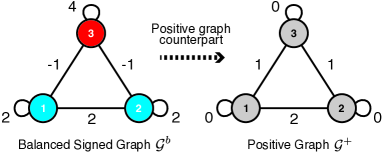
In this paper, we propose a fast GL method that computes a balanced signed graph directly from observed data. Specifically, we extend a previous sparse inverse covariance formulation based on linear programming (LP) called CLIME [27] to compute a balanced signed graph Laplacian given a sample covariance matrix . The Cartwright-Harary Theorem (CHT) [20] states that after appropriately assigning polarities to each graph node , a balanced signed graph has positive / negative edges connecting node-pairs of same / opposing polarities, respectively. See Fig. 1(left) for an illustration of a balanced signed graph with nodes assigned with suitable polarities. The key idea is to add sign constraints on edge weights when node assumes polarity during optimization to maintain graph balance.
After adding edge weight sign constraints, the posed LP (solvable in using an existing LP solver [28]) for node to determine its polarity and edge weights may not feasible for a chosen CLIME parameter that specifies a target sparsity level in . For each LP, we adapt a variant of projections on convex sets (POCS) [29, 30] to determine a suitable in to ensure LP feasibility. Experiments show that our method constructs better quality signed graph Laplacians than previous schemes [25, 26, 22], while enabling reuse of graph filters [31] and GNNs designed for positive graphs for tasks such as signal denoising.
Notation: Vectors and matrices are written in bold lowercase and uppercase letters, respectively. The element and the -th row of a matrix are denoted by and , respectively. The -th element in the vector is denoted by . The square identity matrix of rank is denoted by , the -by- zero matrix is denoted by , and the vector of all ones / zeros of length is denoted by / , respectively. Operator denotes the -norm.
II Preliminaries
II-A Signed Graphs
Denote by an undirected signed graph with node set , edge set , and symmetric weighted adjacency matrix , where weight of edge connecting nodes is . We assume that , can be positive/negative to encode pairwise correlation / anti-correlation, while self-loop weight is non-negative, i.e., . Denote by a diagonal degree matrix, where . We define the standard generalized graph Laplacian matrix222We use the standard generalized graph Laplacian for signed graphs instead of the signed graph Laplacian definition in [19] that requires the absolute value operator. This leads to a simple mapping of eigenvectors of a balanced signed graph Laplacian to ones of a similarity-transformed positive graph Laplacian, and a statistics-driven GL problem formulation extending from [27]. for signed graph as .
II-B Balanced Signed Graphs
A signed graph is balanced if there are no cycles of odd number of negative edges [20]. We rephrase an equivalent definition of balanced signed graphs, known as the Cartwright-Harary Theorem (CHT), as follows.
Theorem 1.
A given signed graph is balanced if and only if its nodes can be polarized into and , such that a positive edge always connects nodes of the same polarity, and a negative edge always connects nodes of opposing polarities.
The edges of a balanced signed graph are consistent.
Definition 2.
A consistent edge is a positive edge connecting two nodes of the same polarity, or a negative edge connecting two nodes of opposing polarities.
For a balanced signed graph with Laplacian , we define its positive graph counterpart with , where denotes a matrix with element-wise absolute value of . Positive graph has its own adjacency matrix333The use of a self-loop of weight equaling to twice the sum of connected negative edge weights is also done in [32]. , where , and , where is a positivity function that returns if and otherwise. Diagonal degree matrix for is defined conventionally, where . Note that adjacency matrix is defined so that the generalized Laplacian is given as
| (1) |
In Fig. 1, we illustrate an example of a balanced signed graph and its positive graph counterpart . In the example, the weights of edges incident on node are , and the self-loop has weight . For the positive graph counterpart, the self-loop on node is .
Laplacian of enjoys a one-to-one mapping of its eigenvectors to those of its positive graph counterpart [21]. Specifically, denote by and the node subsets in with polarity and respectively. We reorder rows / columns of balanced signed graph Laplacian so that nodes in of size are indexed before nodes in of size . Then, using the following invertible diagonal matrix
| (4) |
we see that and are similarity transform of each other:
| (5) | ||||
| (6) | ||||
| (7) |
where in we write , in , and in we apply the definition of generalized graph Laplacian. Thus, and have the same set of eigenvalues, and their eigen-matrices are related via matrix . For the example in Fig. 1, relates to via .
Spectral Graph Filters: Spectral graph filters are frequency modulating filters, where graph frequencies are conventionally defined as the non-negative eigenvalues of a positive graph Laplacian matrix [33]. Thus, to reuse spectral filters designed for positive graphs [13] for a balanced signed graph , it is sufficient to require to be positive semi-definite (PSD), since similarity-transformed shares the same eigenvalues.
II-C Sparse Inverse Covariance Learning
Given a data matrix where and is the -th observation, a sparse inverse covariance matrix (interpretable as a signed graph Laplacian) can be estimated from data via a constrained -minimization formulation called CLIME [27]. In a nutshell, CLIME seeks a positive definite (PD) given a PD sample covariance matrix (assuming zero mean) via a linear programming (LP) formulation:
| (8) |
where is a parameter specifying a target sparsity level. Specifically, (8) computes a sparse (promoted by the -norm objective) that approximates the right inverse of . The -th column of can be computed independently:
| (9) |
where is the canonical vector with one at the -th entry and zero elsewhere. (9) can be solved using an off-the-shelf LP solver such as [28] with complexity . The resulting is not symmetric in general, and [27] computes a symmetric approximation as a post-processing step.
III Balanced Signed Graph Formulation
III-A Optimization Approach
Our goal is to estimate a sparse, PD, balanced signed graph Laplacian directly from empirical covariance matrix . Our algorithm focuses on one node at a time, optimizing its polarity and weights of edges to other nodes . CHT states that in a balanced signed graph, same-/opposing-polarity node pairs are connected by edges of positive/negative weights. Given the edge sign restrictions, for each node , we execute a variant of optimization (9) twice, where the signs of the entries in variable (edge weights ) are restricted for consistency, given an assumed polarity . We then select node ’s polarity corresponding to the smaller of the two objective values.
Specifically, our algorithm is
-
1.
Initialize polarities for all graph nodes .
-
2.
For each column of corresponding to node ,
-
(a)
Assume node ’s polarity or .
-
(b)
Optimize given , ensuring are consistent with the polarities of connected nodes .
-
(c)
Select polarity for node with the smaller objective value.
-
(d)
Update -th column / row of using of node with polarity .
-
(a)
-
3.
Update columns / rows of until convergence.
Note that by simultaneously updating the -th column / row of in step 2(d), remains symmetric.
III-B Linear Constraints for Consistent Edges
To augment CLIME for a balanced signed graph Laplacian, we first construct linear constraints that ensure consistent edges. From Definition 2, we write the following relationship for an edge of the targeted balanced graph w.r.t. node polarities and :
| (10) |
For Laplacian entries , linear constraints for edge consistency can be written as
| (11) |
III-C Optimization of Laplacian Column
III-D Selection of via POCS
| Proposed | GLASSO | CLIME | |||||
|---|---|---|---|---|---|---|---|
| - | Min | Max | Greed | Min | Max | Greed | |
| FM | 0.6679 | 0.4841 | 0.4821 | 0.6117 | 0.4983 | 0.4938 | 0.6405 |
| RE | 0.2854 | 0.4055 | 0.4055 | 0.3705 | 0.3335 | 0.3343 | 0.2898 |
| Methods | Low Pass Filter | Wavelet Filter | GCN | GAT | ||||
|---|---|---|---|---|---|---|---|---|
| Noise Level | ||||||||
| Proposed | 0.2540 | 0.2645 | 0.1670 | 0.1929 | 0.0617 | 0.0691 | 0.0665 | 0.0727 |
| CLIME-Greed | 0.2703 | 0.2812 | 0.1823 | 0.2136 | 0.0747 | 0.0810 | 0.0691 | 0.0737 |
| GLASSO-Greed | 0.4175 | 0.4160 | 0.2177 | 0.2513 | 0.0659 | 0.0746 | 0.0677 | 0.0753 |
| BSigGL | 0.3455 | 0.4129 | 0.2059 | 0.2577 | 0.0761 | 0.0841 | 0.0857 | 0.0944 |
| GGL | 0.3629 | 0.3647 | 0.2061 | 0.2349 | 0.0620 | 0.0711 | 0.0663 | 0.0745 |
For each node , we seek to select so that LP (12) has at least one feasible solution for at least one polarity . We solve the LP feasibility problem efficiently using one variant of projections on convex sets (POCS) [29]: given convex sets that are half-spaces444A half-space is one “half” of the partitioned -dimensional Euclidean space, defined by , where is a hyperplane parameterized by and ., repeated cyclical applications of respective linear projections will converge to an intersection point if one exists. If no intersection point exists, then the same closest points in sets will repeat.
To apply POCS, given the two constraints in (12), we first rewrite them as linear constraints:
| (13) | |||||
where and denote the -th rows of matrix and , respectively. Each constraint in (13) defines a half-space in the form . To project a candidate solution into , we first check if . If so, already. If not, we project onto the hyperplane that defines :
| (14) |
Starting from an initialized , we increase slowly until POCS confirms LP feasibility in . An existing LP solver [28] then solves the feasible LP in .
IV Experiments
We present the results of balanced signed graph learning on both synthetic data and denoising of real data.
Synthetic Data: We randomized a graph based on Erdös–Rényi (ER) model [34] with nodes and edge probability of . Edge weight magnitudes were set randomly in the uniform range . We randomized each node ’s polarity with equal probability. Edge weight signs were set to positive/negative for each node-pair with same/opposing polarities, resulting in a balanced graph. Self-loop on each node was set as , to ensure the resulting graph Laplacian is PD and invertible. signal observations were generated following the Gaussian Markov Random Field (GMRF) model as .
Hourly Air Pressures in Japan555https://www.data.jma.go.jp/stats/etrn/index.php (APJ): This dataset consisted of hourly air pressure records from weather stations in Japan from March 2022 to May 2022. The total observation number was , and we computed a moving average for every hours. The observations at each node were normalized, then contaminated with additive white Gaussian noise (AWGN) with noise levels . Synthetic Data Experiment: We compare the performance of our algorithm against variants of conventional two-step balancing approaches: a precision matrix estimation step followed by a graph balancing step. We employed CLIME [27] or Graphical Lasso (GLASSO) [23] for precision matrix estimation. The three variants of graph balancing methods were: a) MinCut Balancing (Min) [26]: Nodes were polarized based on the min-cut of positive edges, and inconsistent edges were removed. b) MaxCut Balancing (Max) [26]: Nodes were poloarized based on the max-cut of negative edges, and inconsistent edges were removed. c) Greedy Balancing (Greed) [25]: A polarized set was initialized with a random node polarized to , then nodes connected to the set were greedily polarized one-by-one, so that the number of consistent edges to the set was maximized in each polarization.
Result: We numerically evaluate the performance using F-measure (FM), and relative error (RE) in Table I. The values were averaged over 30 runs. The results show that our method outperforms conventional two-step methods in both metrics.
Real Data Experiment: We tested competing methods in signal denoising on the APJ dataset. For positive graph signal denoising, we employed a bandlimited graph low-pass filter (BL), spectral graph wavelets (SGW) [35], graph convolutional net (GCN), and graph attention net (GAT) [36]. We first learned a balanced signed graph Laplacian , which was similarity-transformed (via matrix in (4)) to a positive graph Laplacian as kernel for the denoising algorithms. Each observed noisy signal was also similarity-transformed via for processing on positive graph . For BL, we used a filter that preserves the low-frequency band , where was the maximum eigenvalue of the graph Laplacian. For SGW, we designed the Mexican hat wavelet filter bank for range . The number of frames to cover the interval was set to . For GCN and GAT, we followed the GNN architecture in [36] for signal denoising on positive graphs. We also compared our methods against the balanced signature graph learning method (BSigGL) [22] and a positive graph learning algorithm (GGL) in [37].
Result: We summarize the results in Table II. The values are the average root mean squared errors (RMSE) of the restored signals for filtering methods and normalized MSE for GNN-based methods. Results show that the balanced signed graph learned using our method yields the best performance across all denoising schemes designed for positive graphs.
V Conclusion
We proposed an efficient algorithm to learn a balanced signed graph directly from data. We augment a previous sparse inverse covariance matrix formulation based on linear programming (LP) [27] with additional linear constraints for graph balance. We ensure LP feasibility with a suitable selection of a sparsity parameter via a variant of projections on convex sets (POCS) [29]. In experiments, we showed that our balanced graph learning method enables reuse of spectral filters / GNNs for positive graphs and outperforms previous learning methods.
References
- [1] D. I. Shuman, S. K. Narang, P. Frossard, A. Ortega, and P. Vandergheynst, “The emerging field of signal processing on graphs: Extending high-dimensional data analysis to networks and other irregular domains,” IEEE Signal Process. Mag., vol. 30, no. 3, pp. 83–98, 2013.
- [2] A. Ortega, P. Frossard, J. Kovačević, J. M. F. Moura, and P. Vandergheynst, “Graph Signal Processing: Overview, Challenges, and Applications,” Proc. IEEE, vol. 106, no. 5, pp. 808–828, 2018.
- [3] Y. Tanaka, Y. C. Eldar, A. Ortega, and G. Cheung, “Sampling Signals on Graphs: From Theory to Applications,” IEEE Signal Process. Mag., vol. 37, no. 6, pp. 14–30, 2020.
- [4] T. N. Kipf and M. Welling, “Semi-supervised classification with graph convolutional networks,” in International Conference on Learning Representations, 2017. [Online]. Available: https://openreview.net/forum?id=SJU4ayYgl
- [5] V. Kalofolias, “How to Learn a Graph from Smooth Signals,” in Proc. 19th Int. Conf. Artif. Intell. Stat. PMLR, 2016, pp. 920–929.
- [6] J. Friedman, T. Hastie, and R. Tibshirani, “Sparse inverse covariance estimation with the graphical lasso,” Biostatistics, vol. 9, no. 3, pp. 432–441, 2008.
- [7] D. Thanou, X. Dong, D. Kressner, and P. Frossard, “Learning heat diffusion graphs,” IEEE Trans. Signal Inf. Process. Netw., vol. 3, pp. 484–499, 2016.
- [8] G. Mateos, S. Segarra, A. G. Marques, and A. Ribeiro, “Connecting the dots: Identifying network structure via graph signal processing,” IEEE Signal Process. Mag., vol. 36, no. 3, pp. 16–43, 2019.
- [9] X. Dong, D. Thanou, M. Rabbat, and P. Frossard, “Learning graphs from data: A signal representation perspective,” IEEE Signal Process. Mag., vol. 36, no. 3, pp. 44–63, 2019.
- [10] S. Bagheri, T. T. Do, G. Cheung, and A. Ortega, “Spectral graph learning with core eigenvectors prior via iterative GLASSO and projection,” IEEE Transactions on Signal Processing, vol. 72, pp. 3958–3972, 2024.
- [11] M. Onuki, S. Ono, M. Yamagishi, and Y. Tanaka, “Graph Signal Denoising via Trilateral Filter on Graph Spectral Domain,” IEEE Trans. Signal Inf. Process. Netw., vol. 2, no. 2, pp. 137–148, 2016.
- [12] J. Pang and G. Cheung, “Graph Laplacian regularization for inverse imaging: Analysis in the continuous domain,” in IEEE Trans. Image Process., vol. 26, no.4, April 2017, pp. 1770–1785.
- [13] D. I. Shuman, “Localized spectral graph filter frames: A unifying framework, survey of design considerations, and numerical comparison,” IEEE Signal Processing Magazine, vol. 37, no. 6, pp. 43–63, 2020.
- [14] X. Liu, G. Cheung, X. Wu, and D. Zhao, “Random walk graph Laplacian based smoothness prior for soft decoding of JPEG images,” in IEEE Trans. Image Process., vol. 26, no.2, February 2017, pp. 509–524.
- [15] F. Chen, G. Cheung, and X. Zhang, “Manifold graph signal restoration using gradient graph laplacian regularizer,” IEEE Transactions on Signal Processing, vol. 72, pp. 744–761, 2024.
- [16] Y. Hou, J. Li, and Y. Pan, “On the Laplacian Eigenvalues of Signed Graphs,” Linear Multilinear Algebra, vol. 51, no. 1, pp. 21–30, 2003.
- [17] L. Wu, X. Ying, X. Wu, A. Lu, and Z.-H. Zhou, “Spectral Analysis of k-Balanced Signed Graphs,” in Adv. Knowl. Discov. Data Min., ser. Lecture Notes in Computer Science, J. Z. Huang, L. Cao, and J. Srivastava, Eds. Berlin, Heidelberg: Springer, 2011, pp. 1–12.
- [18] J. Kunegis, S. Schmidt, A. Lommatzsch, J. Lerner, E. W. De Luca, and S. Albayrak, “Spectral Analysis of Signed Graphs for Clustering, Prediction and Visualization,” in Proceedings of the 2010 SIAM International Conference on Data Mining (SDM), ser. Proceedings. Society for Industrial and Applied Mathematics, 2010, pp. 559–570.
- [19] T. Dittrich and G. Matz, “Signal Processing on Signed Graphs: Fundamentals and Potentials,” IEEE Signal Process. Mag., vol. 37, no. 6, pp. 86–98, 2020.
- [20] F. Harary, “On the notion of balance of a signed graph.” Mich. Math. J., vol. 2, no. 2, pp. 143–146, 1953.
- [21] C. Yang, G. Cheung, and W. Hu, “Signed Graph Metric Learning via Gershgorin Disc Perfect Alignment,” IEEE Trans. Pattern Anal. Mach. Intell., vol. 44, no. 10, pp. 7219–7234, 2022.
- [22] G. Matz, C. Verardo, and T. Dittrich, “Efficient learning of balanced signature graphs,” in ICASSP 2023 - 2023 IEEE International Conference on Acoustics, Speech and Signal Processing (ICASSP), 2023, pp. 1–5.
- [23] R. Mazumder and T. Hastie, “The graphical lasso: New insights and alternatives,” Electron J Stat, vol. 6, pp. 2125–2149, 2012.
- [24] J. Akiyama, D. Avis, V. Chvátal, and H. Era, “Balancing signed graphs,” Discrete Applied Mathematics, vol. 3, no. 4, pp. 227–233, 1981.
- [25] C. Dinesh, S. Bagheri, G. Cheung, and I. V. Bajić, “Linear-Time Sampling on Signed Graphs Via Gershgorin Disc Perfect Alignment,” in ICASSP 2022 - 2022 IEEE Int. Conf. Acoust. Speech Signal Process. ICASSP, 2022, pp. 5942–5946.
- [26] H. Yokota, J. Hara, Y. Tanaka, and G. Cheung, “Signed graph balancing with graph cut,” in 2023 31st European Signal Processing Conference (EUSIPCO), 2023, pp. 1853–1857.
- [27] T. Cai, W. Liu, and X. Luo, “A constrained minimization approach to sparse precision matrix estimation,” Journal of the American Statistical Association, vol. 106, no. 494, pp. 594–607, 2011.
- [28] S. Jiang, Z. Song, O. Weinstein, and H. Zhang, “Faster dynamic matrix inverse for faster lps,” 2020.
- [29] S. Kaczmaarz, “Angenäherte auflosung von systemen linearer gleichungen,” Bulletin International de l’Académie Polonaise des Sciences et des Lettres. Classe des Sciences Mathématiques et Naturelles. Série A, Sciences Mathématiques, vol. 35, p. 355–357, 1937.
- [30] R. Escalante and M. Raydan, Alternating Projection Methods. USA: Society for Industrial and Applied Mathematics, 2011.
- [31] I. Pesenson, “Variational Splines and Paley–Wiener Spaces on Combinatorial Graphs,” Constr Approx, vol. 29, no. 1, pp. 1–21, 2009.
- [32] W.-T. Su, G. Cheung, and C.-W. Lin, “Graph Fourier transform with negative edges for depth image coding,” in 2017 IEEE International Conference on Image Processing (ICIP), 2017, pp. 1682–1686.
- [33] G. Cheung, E. Magli, Y. Tanaka, and M. K. Ng, “Graph spectral image processing,” in Proceedings of the IEEE, vol. 106, no.5, May 2018, pp. 907–930.
- [34] P. Erdös and A. Rényi, “On random graphs i,” Publicationes Mathematicae Debrecen, vol. 6, pp. 290–297, 1959.
- [35] D. K. Hammond, P. Vandergheynst, and R. Gribonval, “Wavelets on graphs via spectral graph theory,” Applied and Computational Harmonic Analysis, vol. 30, no. 2, pp. 129–150, 2011.
- [36] S. Rey, S. Segarra, R. Heckel, and A. G. Marques, “Untrained graph neural networks for denoising,” arXiv preprint arXiv:2109.11700, 2021.
- [37] H. E. Egilmez, E. Pavez, and A. Ortega, “Graph Learning From Data Under Laplacian and Structural Constraints,” IEEE J. Sel. Top. Signal Process., vol. 11, no. 6, pp. 825–841, 2017.