Analog-Based Forecasting of Turbulent Velocity:
Relationship between Predictability and Intermittency

Abstract

This study evaluates the performance of analog-based methodologies to predict the longitudinal velocity in a turbulent flow. The data used comes from hot wire experimental measurements from the Modane wind tunnel. We compared different methods and explored the impact of varying the number of analogs and their sizes on prediction accuracy. We illustrate that the innovation, defined as the difference between the true velocity value and the prediction value, highlights particularly unpredictable events that we directly link with extreme events of the velocity gradients and so to intermittency. This result indicates that while the estimator effectively seizes linear correlations, it fails to fully capture higher-order dependencies. The innovation underscores the presence of intermittency, revealing the limitations of current predictive models and suggesting directions for future improvements in turbulence forecasting.

I Introduction

For a given temporal stochastic process $X$, Cramér defined innovation to describe the new random inputs into the system and to quantify the unpredictability in the time evolution of $X$  cramerLinearPredictionProblem1960 ; doobStochasticProcesses1953 . For a deterministic dynamical system, if a solution exists and is known, the lack of noise leads to a vanishing innovation. However, in chaotic systems, innovation rarely vanishes and can be used to quantify the degree of predictability of the process and to identify unpredictable localized events related to the system’s dynamics.

Fluid turbulence is one example of a chaotic system with very complex multiscale dynamics, in which the velocity field is impossible to derive deterministically peinkeChaosFractalsTurbulence1993 ; crisantiIntermittencyPredictabilityTurbulence1993 ; crisantiPredictabilityVelocityTemperature1993 ; aurellPredictabilitySystemsMany1996 ; boffettaPredictabilityChaoticSystems1998 ; boffettaChaosPredictabilityHomogeneousIsotropic2017 . Turbulent velocity presents long-range correlations, indicating non-local interactions frischTurbulenceLegacyKolmogorov1995b , and intermittency leads to extreme events in the velocity gradients frischTurbulenceLegacyKolmogorov1995b ; meneveauMultifractalNatureTurbulent1991 . Additionally, in numerical experiments, noise is present due to numerical solver approximations and machine precision while in physical experiments, noise is naturally present within the sensors or experimental procedures themselves, and the observations are usually limited to some coordinates of the velocity field only. As a consequence, a minimal level of unpredictability is always present in a turbulent velocity signal.

We propose to characterize the predictability of turbulent velocity in terms of innovation, highlighting that difficult-to-predict events are related to bursts in velocity gradients and thus to intermittency. In this context, we adapt analog-based estimatorslorenzAtmosphericPredictabilityRevealed1969a previously used in meteorological doolNewLookWeather1989a ; tothLongRangeWeatherForecasting1989 and dynamical systems applications sugiharaNonlinearForecastingWay1990 to predict the next value in a hot-wire velocity measurement from a grid turbulence experiment in the Modane wind tunnel kahalerrasIntermittencyReynoldsNumber1998a . We compute the corresponding innovation as the difference between the real signal and its prediction. We then analyze the statistical properties of the velocity, velocity increment, innovation, and the cumulative sum of innovations by examining their second-order structure function and flatness. On the one hand, the second order structure function is a second-order statistic that characterizes the energy distribution across scales. On the other hand, the flatness is a higher-order statistic that characterizes the significance of extreme events across scales.

While the analog-based innovation predictions can effectively capture and predict non-extreme dynamics by removing some linear dependencies, extreme events in velocity gradients due to intermittency are not accurately predicted by the analog method. This method falls short in accounting for higher-order dependencies. The innovation process shows a nearly white spectrum with a non-Gaussian, fat-tailed probability distribution and retains higher-order dependencies. Extreme events in innovation are localized in time and appear concomitantly with extreme velocity gradient events, indicating that intermittency introduces unpredictability into the system.

This article is structured into three sections. In section Turbulence & Intermittency we discuss intermittency, its characterization, and the turbulent data used. Section Innovation introduces the new proposed framework and the estimators we compute. Finally, section Results evaluates the performance of the different estimators and discusses the statistics of innovation on real experimental data.

II Turbulence & Intermittency

The Richardson cascade picture of three-dimensional turbulence identifies three domains of scale: the integral domain, which contains the large scales where energy is injected; the inertial range, where energy cascades from large to small scales; and the dissipative domain where energy is dissipated at smaller scales.

In the case of three-dimensional fully developed turbulence, the multifractal formalism frischSingularityStructureFully1985 ; frischTurbulenceLegacyKolmogorov1995b ; paladinAnomalousScalingLaws1987 describes in the inertial domain a power law behavior of the structure functions $S_{p}(l)$ of the turbulent velocity field as a function of the scale:

$$S_{p}(l)=\mathbb{E}[(\delta_{l}v)^{p}]\propto l^{\zeta(p)}$$ (1)

where $\delta_{l}v=v(x+l)-v(x)$ is the velocity increment of size $l$ and $\zeta(p)$ is the scaling exponent.

The Kolmogorov’s 1941 (K41) theory kolmogorovLocalStructureTurbulence1991 originally proposed a linear scaling exponent $\zeta(p)=ph$, with a single Holder exponent $h=\frac{1}{3}$ i.e. a monofractal velocity field. This model does not take into account the intermittency phenomenon highlighted by experiments gagneNewUniversalScaling1990 ; kahalerrasIntermittencyReynoldsNumber1998a . Intermittency is characterized by a deformation of the probability density function of the velocity increments from Gaussian at large scales to non-Gaussian with heavy tails at small scales castaingVelocityProbabilityDensity1990 . This behavior reflects the presence of extreme events, which become more significant at smaller scales. It implies multifractality: a non-linear scaling exponent $\zeta(p)$ with a dependancy of h upon p $\zeta(p)=ph(p)$. An intermittent model of turbulence was proposed by Kolmogorov and Obukhov (KO62)  kolmogorovRefinementPreviousHypotheses1962 ; obukhovSpecificFeaturesAtmospheric1962 and later studied within the multifractal formalism chevillardPhenomenologicalTheoryEulerian2012 ; castaingVelocityProbabilityDensity1990 ; paladinAnomalousScalingLaws1987 ; castaingLogsimilarityTurbulentFlows1993 ; delourIntermittency1DVelocity2001a ; meneveauMultifractalNatureTurbulent1991 .

The energy distribution across scales is characterized by the second-order structure function $S_{2}(l)$ which, for scales in the inertial domain, is proportional to $l^{2/3}$ up to intermittent corrections frischTurbulenceLegacyKolmogorov1995b . $S_{2}(l)$ characterizes second-order statistics of the turbulent velocity field in the same way as autocorrelation and power spectrum frischTurbulenceLegacyKolmogorov1995b .

The flatness characterizes the relative importance of extreme events and allows for a measure of the deformation of the PDF. It is defined for a given scale $l$ as

$$F(l)=\frac{S_{4}(l)}{3S_{2}(l)^{2}}$$ (2)

It thus characterizes higher-order statistics of velocity. In a monofractal Gaussian field, the flatness remains constant across scales and is equal to $1$. In contrast, turbulence shows an increasing flatness with decreasing scale $l$, indicating a higher prevalence of extreme events or bursts at smaller scales dubrulleKolmogorovCascades2019 ; buariaExtremeVelocityGradients2019 ; moffattExtremeEventsTurbulent2021 . The increased flatness at smaller scales due to the departure from Gaussian statistics is a key indicator of intermittency.

II.1 Modane Turbulent Velocity Dataset

We use an Eulerian longitudinal velocity measurement from an experimental grid turbulence setup in the Modane wind tunnel kahalerrasIntermittencyReynoldsNumber1998a . The full velocity measure spans $1000$ seconds with a sampling frequency of $f_{s}=25$ kHz. Velocity measurements were obtained using hot-wire anemometry. The Taylor scale Reynolds number of the flow is $R_{\lambda}=2500$.

To relate temporal measurements to spatial properties, we employ Taylor’s hypothesis of frozen turbulence, which allows us to interpret temporal variations in the velocity signal as spatial variations using $v(x,t)=v(x-Vt,0)$ , where $v$ is the velocity, $x$ is the space coordinate in the longitudinal direction, defined along the mean velocity of the flow, $t$ is the time coordinate and $V=20.5ms^{-1}$ is the mean velocity of the flow.

From previous studies, the integral scale of the flow is $L=2350dl$ and the Kolmogorov scale kolmogorovLocalStructureTurbulence1941a of the flow is $\eta=5dl$ granero-belinchonScalingInformationTurbulence2016 , where $dl=V/f_{s}$.

In the following, all results are presented in function of $t/T$ with $T=L/V$.

III Innovation

III.1 Theoretical Description

For a stochastic process $X=\{x_{t}\}$ sampled at intervals equally separated by $dt$, we define the innovation $\epsilon_{t}$ as:

$$\epsilon_{t}=x_{t}-\mathbb{E}[x_{t}|x_{-\infty:t-dt}]$$ (3)

where $\mathbb{E}[x_{t}|x_{-\infty:t-dt}]$ is the expected value of $x_{t}$ conditioned on its complete past $x_{-\infty:t-dt}$.

We interpret $\epsilon_{t}$ as the novel, unpredictable component of $x_{t}$ at time $t$ cramerLinearPredictionProblem1960 ; doobStochasticProcesses1953 . Thus, innovation acts as a limit to the error of an optimal prediction, providing insight into the degree of unpredictability of the system as a function of time.

Very interestingly, innovation can point out specific unpredictable events localized in time.

In practice, the expected value $\mathbb{E}[x_{t}|x_{-\infty:t-dt}]$ cannot be conditioned on an infinite past and we restrict the conditioning on a finite past interval $t\in[t-pdt,t-dt]$, leading to the approximation:

$$\epsilon_{t}^{(p)}=x_{t}-\mathbb{E}[x_{t}|x_{t-pdt:t-dt}]$$ (4)

where $p$ indicates the finite duration of the past horizon.

III.2 Analogs

For a given time $t$, we consider the temporal sub-sequence $\vec{x}^{(p)}_{t}$ of size $p$ of the stochastic process $X$ as:

$$\vec{x}_{t}^{(p)}=\begin{pmatrix}x_{t-dt}\\ \vdots\\ x_{t-pdt}\end{pmatrix}$$ (5)

Two such sub-sequences $\vec{x}_{t}^{(p)}$ and $\vec{x}_{t^{\prime}}^{(p)}$ considered at two different times $t$ and $t^{\prime}$ are called analogs if they are close enough in terms of some given $p$-dimensional distance.

Based on Poincaré’s theorem poincareProblemeTroisCorps1890a , we assume that 1) analogs exist if the time series if sufficiently long; and 2) close analogs will lead to close successors. Then for a given $t$, the set of successors $x_{t^{\prime}}$ of the analogs $\vec{x}_{t^{\prime},p}$ of $\vec{x}_{t}^{(p)}$ can be used to predict the successor $x_{t}$. This approach relies on the similarity of past sequences and their subsequent outcomes for making predictions.

In the context of the present study, analog forecasting serves as a methodological framework for estimating the expected value $\mathbb{E}[x_{t}|x_{t-pdt:t-dt}]$ that appears in the definition of innovation.

III.3 Analog-based predictions and innovations

Given $\vec{x}_{t}^{(p)}$ and a fixed integer $k$, we define the analogs of $\vec{x}_{t}^{(p)}$ as the set $\{\vec{x}_{t^{\prime}_{i}}^{(p)}\}_{1\leq i\leq k}$ of the $k$ historical sequences with $t^{\prime}_{i}<t$ that are the closest to $\vec{x}_{t}^{(p)}$ in terms of the Euclidean distance, as suggested in platzerUsingLocalDynamics2021c ; lguensatAnalogDataAssimilation2017a .

III.4 Average

The original method for analog prediction computes a weighted average of the successors $\{x_{t^{\prime}_{i}}\}_{1\leq i\leq k}$ of the analogs  kruizingaUseAnalogueProcedure1983 ; monacheKalmanFilterAnalog2011 . This leads to the Average prediction $\hat{x_{t}}^{(p)}$:

$$\hat{x_{t}}^{(p)}=\frac{1}{k}\sum_{i=1}^{k}w_{ii}x_{t^{\prime}_{i}}$$ (6)

with the corresponding innovation $\hat{\epsilon}_{t}^{(p)}=x_{t}-\hat{x_{t}}$. The weights $w_{ii}$ are defined as the components of a diagonal weight matrix $\bm{W}$:

$$w_{ii}=\frac{e^{-||\vec{x}_{t}^{(p)}-\vec{x}_{t^{\prime}_{i}}^{(p)}||/\lambda}}{\sum_{j=1}^{k}e^{-||\vec{x}_{t}^{(p)}-\vec{x}_{t^{\prime}_{j}}^{(p)}||/\lambda}}$$ (7)

with $\lambda=\text{median}(\{||\vec{x}_{t}^{(p)}-\vec{x}_{t^{\prime}_{i}}^{(p)}||\}_{1\leq i\leq k})$, following the work of  platzerUsingLocalDynamics2021c ; lguensatAnalogDataAssimilation2017a .

This averaging method tends to draw predictions towards the average of the $k$ successors, resulting in forecasts that are more inaccurate in unexplored regionslguensatAnalogDataAssimilation2017a . It nevertheless gives a simple first estimator that we compare to more sophisticated one below.

III.5 Linear Regression (LR)

Following platzerUsingLocalDynamics2021c , we then make an analog-based prediction using a weighted linear regression performed on each analog successor $x_{t^{\prime}_{i}}$, in order to identify a relationship between analogs and successors.

For a given number $k$ of analogs, the minimization problem can be written as $\min\limits_{\beta_{t}}||\vec{x}-\bm{W}\bm{X_{p}}\beta_{t}||$ where:

• $\vec{x}$ is the vector of analogs’ successors:

  $$\vec{x}=\begin{pmatrix}x_{t_{1}^{\prime}}\\ \vdots\\ x_{t_{k}^{\prime}}\end{pmatrix},$$ (8)

• $\bm{X_{p}}$ is a $k\times(p+1)$ matrix containing all analog vectors:

  $$\bm{X_{p}}=\begin{pmatrix}1&x_{t^{\prime}_{1}-dt}&\ldots&x_{t^{\prime}_{1}-pdt}\\ \vdots&\vdots&&\vdots\\ 1&x_{t^{\prime}_{k}-dt}&\ldots&x_{t^{\prime}_{k}-pdt}\end{pmatrix}$$ (9)

  with a first line of ones added for regularization.

• $\bm{W}$ is a $k\times k$ diagonal matrix which specifies the weight of each analog. The non-zero elements $w_{ii}$ of $\bm{W}$ are defined using eq.7.

• $\beta_{t}$ is the coefficients vector of the weighted linear regression that depend on $t$ through the definition of the analogs, that we search for.

The ordinary least squares estimator for the minimization gives:

$$\hat{\beta_{t}}=(\bm{X_{p}}^{T}\bm{W}\bm{X_{p}})^{-1}\bm{X_{p}}^{T}\bm{W}\vec{x}$$ (10)

The analog prediction then reads:

$$\hat{x_{t}}^{(p)}\equiv\hat{\beta}_{t}\vec{x}_{t}^{(p)}$$ (11)

with the corresponding innovation $\hat{\epsilon}_{t}^{(p)}=x_{t}-\hat{\beta}_{t}\vec{x}_{t}^{(p)}$.

This ”LR” approach in phase space establishes a relationship from past states to their successors based on historical analogs. It has two parameters: the number $k$ of neighbors and the dimension $p$ of the sub-sequences. Note that for the inversion (eq.10) to be possible, one should have $k\geq p$.

III.6 Normalized LR

One can focus on trends rather than values by removing the mean value of the sub-sequences, allowing the analog search to prioritize patterns over analogs’ values barnettMultifieldAnalogPrediction1978 . This method is thus identical to ”LR” method after replacing all coordinates $x_{t_{j}}$ of sub-sequences $\vec{x}_{t}^{(p)}$ by $x_{t_{j}}-\overline{\vec{x}_{t}^{(p)}}$ with $\overline{\vec{x}_{t}^{(p)}}\equiv\frac{1}{p}\sum_{1\leq j\leq p}x_{t-jdt}$.

IV Results

IV.1 Analogs Prediction

In this section, we compare the performance of the three analog-based predictions presented here above. We also evaluate the impact of $k$ and $p$ in the performance, in order to determine the optimal values for $k$ and $p$.

We compute the corresponding innovations $\epsilon_{t}^{(p)}$ for different methodologies and $k$ and $p$ combinations. This is done on $n_{\rm real}=10$ realizations of length $N=2^{21}\simeq 900T$ samples of the Modane turbulent velocity $v$. (see fig.1) The database containing the historical record for analog searching is chosen to precede and not overlap with the portion over which the predictions and innovations are computed and it contains a total of $N_{\rm a}=N$ samples, where $N_{\rm a}$ has been selected to ensure that further increasing the size of the historical record does not significantly affect the results. Overlap between analogs is not permitted, ensuring that the selected analogs are distinct. The results are computed over the $n_{\rm real}$ realizations.

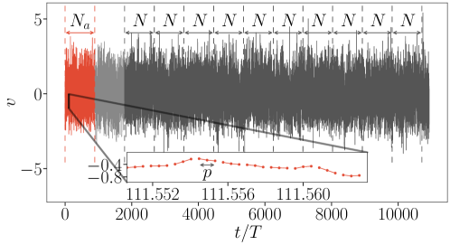
Figure 1: Visualization of Modane turbulent velocity data usage for the innovation $\epsilon_{t}^{(p)}$. The first red section of size $N_{\rm a}$ represents the historical record used for analog search. The subsequent ten black sections are the $n_{\rm real}=10$ realizations of size $N$ over which the innovation is computed. Vertical dashed lines indicate the boundaries of the historical record and of the realizations. The inset shows a zoom of the historical record with non-overlapping analogs candidates and a highlighted analog length $p=3$.

The performance of a prediction $\hat{x_{t}}$ is quantified with the variance of its corresponding innovation $\epsilon_{t}^{(p)}=x_{t}-\hat{x_{t}}^{(p)}$: a perfect prediction would yield zero variance. On the contrary, the naive prediction $\hat{v_{t}}=v_{t-dt}$ assumes a locally constant speed and hence doesn’t account for any dynamics or even any change in the process. It leads to the innovation $\epsilon^{0}_{t}$:

$$\epsilon^{0}_{t}=v_{t}-v_{t-dt}=\delta_{dt}v$$ (12)

which is nothing but the increment $\delta_{dt}v$. As a consequence, we can use the increment as a baseline of the behavior of the innovation $\epsilon_{t}^{(p)}$ for the three analog-prediction methods presented earlier.

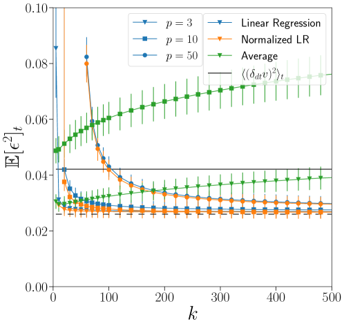
Figure 2: Standard deviation of the innovation $\epsilon_{t}^{(p)}=v_{t}-\hat{v_{t}}^{(p)}$ as a function of the number $k$ of neighbors used in the kNN algorithm. The performance is shown for different sizes of the past: $p=3,10,50$ and for different methods: Linear Regression (blue), Normalized LR (orange), Averaging LR (green). Vertical lines correspond to the average value and errorbars to the standard deviation computed over $n_{\rm real}$ realizations. Increment variance (continuous black line) is present as a baseline for informative prediction, see (eq.12), and a dashed line is present to highlight the minimum value towards which the estimator converges.

In Figure 2 we compare the performance of the three analog prediction methods as a function of $k$ for different values of $p$. ”Normalized LR” configuration (orange) consistently shows the lowest variance in the innovation, indicating superior performance. Regular ”LR” (blue) yields similar results. For these two estimators: 1) the variance increases when $p$ increases due to the curse of dimensionality leading to increased computational complexity and convergence issues and 2) the variance decreases when $k$ increases until reaching a plateau at $\mathbb{E}_{t}[\epsilon^{2}]=0.026$. ”Average” (green) method without linear regression shows higher variance which increases with the number $k$ of neighbors.

Increasing the size $p$ of the sub-sequences over $p=3$ does not improve performance, even when $k$ is accordingly increased. This is because three-point statistics already capture most of the dynamics of turbulent flows peinkeFokkerPlanckApproach2019b .

The lower variance of innovation compared to the one of the increment (horizontal continuous black line) indicates that predictions are indeed containing relevant information on the dynamics. The existence of a minimum plateau should be interpreted cautiously since we are using only a single-point velocity measurement, which may not probe the full 3D complexity of turbulence. In line with previous works lguensatAnalogDataAssimilation2017a , using linear regression for analogs significantly enhances prediction accuracy, with the linear regression model far outperforming averaging methods.

Based on this performance analysis, we use the ”Normalized LR” method in the following, with $p=3$ and $k=70$.

IV.2 Innovation Statistics

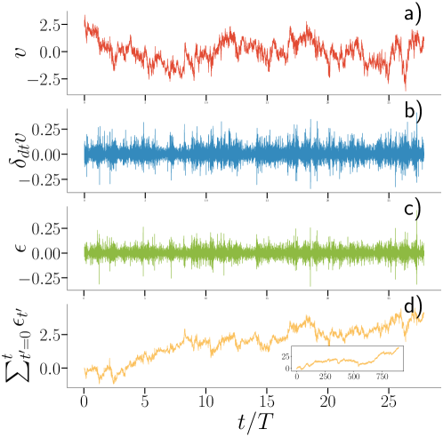
Figure 3: Time series of the Modane velocity $v$ (a), its smallest increment $\delta_{dt}v$ (b), the innovation $\epsilon$ (c), and the cumulative sum of innovation $\sum_{t^{\prime}=0}^{t}\epsilon_{t^{\prime}}^{(p)}$ (d). The insert shows the cumulative sum of innovation over a longer duration.

Figures 3a) and 3b) show respectively the typical evolution of the Modane velocity $v$ and of its increment $\delta_{dt}v$ over multiple integral scales. The increment exhibits intermittent behavior with calm regions and bursty regions that highlight its non-Gaussianity. Figures 3c) and 3d) show respectively the innovation $\epsilon_{t}^{(p)}$ and its cumulative sum $\sum_{t^{\prime}=0}^{t^{\prime}=t}\epsilon_{[}t^{\prime}]^{(p)}$. The innovation mirrors the behavior of the increment but with reduced variance. The concomitant occurence of bursts in both the increment and the innovation time series suggests that extreme events in the increments induced by intermittency lead to an increase in the unpredictability of the velocity values $v_{t}$ knowing their past $(v_{t-dt},v_{t-2dt},v_{t-3dt})$. This is coherent with previous results illustrating the challenge of predicting extreme events  dubrulleKolmogorovCascades2019 ; buariaExtremeVelocityGradients2019 ; moffattExtremeEventsTurbulent2021 . The cumulative sum of the innovation is non-stationary and seems to behave like a random walk, which might indicate that the linear part of the dynamics is correctly predicted in $\hat{v_{t}}^{(p)}$ and therefore removed from the innovation $\epsilon_{t}^{(p)}$.

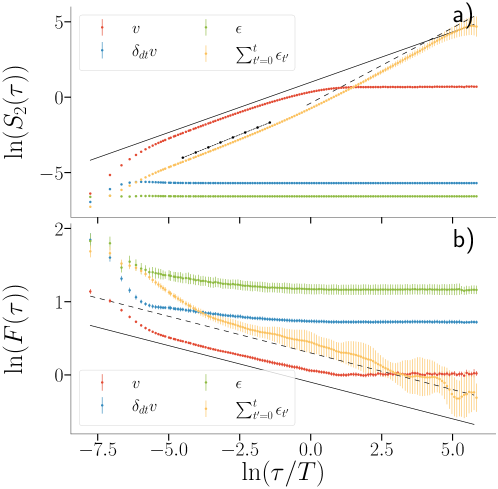
Figure 4: Modane moments: a) second-order structure function $S_{2}(\bullet)$ and b) flatness $S_{4}(\bullet)/3\cdot S_{2}(\bullet)$ for the velocity $v$ (red), the associated smallest increment $\delta_{dt}v$ (blue), innovation $\epsilon$ (green), and innovation sum (yellow). Lines correspond to the average value and errorbars to the standard deviation computed over $n_{\rm real}$ realizations. Computation are done over 10 realizations, each of 892 integral scales. The black lines correspond to power laws: a) continuous:$(\tau/T)^{2/3}$, dashed:$(\tau/T)^{1}$, round markers :$(\tau/T)^{0.77}$ and b) continuous and dashed:$(\tau/T)^{-0.1}$ with different offsets.

Figures 4a) and 4b) present the evolution of the second-order structure function and the flatness, with the time-scale $\tau$ of the increment, for the Modane turbulent velocity $v_{t}$ (red), its increment $\delta_{dt}v$ (blue), the innovation $\epsilon_{t}^{(p)}$ (green), and its cumulative sum (yellow). We relate our results obtained in time to Kolmogorov-Obukhov theories in space using Taylor’s hypothesis kolmogorovRefinementPreviousHypotheses1962 ; obukhovSpecificFeaturesAtmospheric1962 .

The logarithm of the second order structure function $\ln(S_{2}(\tau/T))$ of the increment $\delta_{dt}v$ and the innovation $\epsilon$ (blue and green curves respectively) behave very similarly with the time-scale $\tau$. However, it is completely constant across scales for the innovation while it increases at small scales for the increment, until reaching a plateau.

This increase of the second order structure function $S_{2}$ of the increment at small scales reveals the existence of linear correlations within this process. In contrast, the flat behavior of $S_{2}$ for the innovation (in green) indicates that linear correlations have been eliminated and accurately predicted by the analog method.

For the velocity (in red), we recognize the three following distinct regions: the integral domain at larger scales, characterized by a plateau and the largest value of $S_{2}$; the inertial range with the $\tau^{2/3}$ scaling from K41 theory (eq.1) with $\zeta(2)=2h$ and $h=1/3$) up to intermittent corrections; and the dissipative domain at smaller scales with a $(\tau/T)^{2}$ scaling. For the cumulative sum of the innovation (in yellow), we observe two distinct regions with different power laws: one with an exponent close to ${0.7}$ from the smallest scales up to $\tau\sim T$ and one with an exponent $1$ at larger scales, identical to a Brownian motion.

Finally, the logarithm of the flatness $\ln(F(\tau/T))$ is presented in fig.4b). The flatness of the increments $\delta_{dt}v$ (in blue) and of the innovation $\epsilon$ (in green) is always larger than one, indicating non-Gaussian behavior at all scales. The flatness of the innovation is larger because simple linear correlations have been predicted, which reduces $S_{2}$. This implies that the unpredicted extreme events due to intermittency have a greater relative impact, resulting in increased flatness. For the velocity (in red) the flatness tends to 1 at large scales, indicating Gaussian behavior, while being substantially larger at smaller scales, revealing intermittency granero-belinchonKullbackLeiblerDivergenceMeasure2018 . The cumulative sum of the innovation (in yellow) shows a power-law behavior for scales larger than $\ln(\tau/T)\sim-3$ with an exponant close to $-0.1$. For smaller scales, the evolution of the flatness is faster. Such behavior indicates the persistence of higher-order correlations within the innovation signal, despite the removal of most, if not all, linear correlations.

V Conclusion

In this study, we used analog-based predictions of turbulent velocity measurements from the Modane wind tunnel and computed the innovation in order to analyze the predictability of turbulent velocity. A first application confirmed that linear regression-based analog prediction better accounts for complex dynamics such as turbulence, compared to the standard averaging method, as suggested by state-of-the-art studies. Our analysis then demonstrated that extreme events in the turbulent velocity gradient correspond to extreme events in the innovation, indicating a direct relationship between intermittency-related bursts of the velocity signal and harder to predict velocity values.

Moreover, a multi-scale analysis revealed that the analog-based estimator of turbulent velocity effectively predicts and removes most linear dependencies in the turbulent velocity signal, as evidenced by the flat second-order structure function of the corresponding innovation. The second-order structure function of the cumulative sum of the innovation does not exhibit the typical dissipative and integral domains. Instead, it shows two distinct regions with different power laws: one with a slope close to 0.7 and another with a slope 1. This suggests that while the estimator captures linear dynamics, it struggles with high-order dependencies. The flatness analysis further confirms that high-order dependencies remain largely intact, as indicated by the same power law of exponent -0.1 for the cumulative sum of the innovation as for the turbulent velocity itself. These findings highlight the limitations of the current analog-based estimator in fully capturing high-order interactions and extreme events. Future research should focus on developing improved methods to predict high-order interactions and better capture the full complexity of turbulent flows.

The analog-based prediction methods and calculation of innovation were implemented using Python. The code is available in our GitLab repository for transparency and reproducibility: https://gitlab.imt-atlantique.fr/e22froge/multi-scale-causality

- (1) H. Cramér, On the linear prediction problem for certain stochastic processes, Arkiv för Matematik 4 (1) (1960) 45–53. doi:10.1007/BF02591321.
- (2) J. L. Doob, Stochastic Processes, Wiley, 1953.
- (3) J. Peinke, M. Klein, A. Kitte, A. Okninsky, J. Parisi, . E. Roessler, On chaos, fractals and turbulence, Physica Scripta T49 (1993) 672–676.
- (4) A. Crisanti, M. H. Jensen, A. Vulpiani, G. Paladin, Intermittency and predictability in turbulence, Physical Review Letters 70 (2) (1993) 166–169. doi:10.1103/PhysRevLett.70.166.
- (5) A. Crisanti, M. H. Jensen, G. Paladin, A. Vulpiani, Predictability of velocity and temperature fields in intermittent turbulence, Journal of Physics A: Mathematical and General 26 (23) (1993) 6943. doi:10.1088/0305-4470/26/23/034.
- (6) E. Aurell, G. Boffetta, A. Crisanti, G. Paladin, A. Vulpiani, Predictability in systems with many characteristic times: The case of turbulence, Physical Review E 53 (3) (1996) 2337–2349. doi:10.1103/PhysRevE.53.2337.
- (7) G. Boffetta, A. Celani, Predictability in chaotic systems and turbulence, Le Journal de Physique IV 08 (PR6) (1998) Pr6–146. doi:10.1051/jp4:1998619.
- (8) G. Boffetta, S. Musacchio, Chaos and Predictability of Homogeneous-Isotropic Turbulence, Physical Review Letters 119 (5) (2017) 054102. doi:10.1103/PhysRevLett.119.054102.
- (9) U. Frisch, Turbulence: The Legacy of A.N. Kolmogorov, Cambridge University Press, 1995.
- (10) C. Meneveau, K. R. Sreenivasan, The multifractal nature of turbulent energy dissipation, Journal of Fluid Mechanics 224 (1991) 429–484. doi:10.1017/S0022112091001830.
- (11) E. N. Lorenz, Atmospheric Predictability as Revealed by Naturally Occurring Analogues, Journal of the Atmospheric Sciences 26 (4) (1969) 636–646.
- (12) H. M. van den Dool, A New Look at Weather Forecasting through Analogues, Monthly Weather Review 117 (10) (1989) 2230–2247.
- (13) Z. Toth, Long-Range Weather Forecasting Using an Analog Approach, Journal of Climate 2 (6) (1989) 594–607.
- (14) G. Sugihara, R. M. May, Nonlinear forecasting as a way of distinguishing chaos from measurement error in time series, Nature 344 (6268) (1990) 734–741. doi:10.1038/344734a0.
- (15) H. Kahalerras, Y. Malecot, Y. Gagne, B. Castaing, Intermittency and Reynolds number, Physics of Fluids 10 (1998) 910–921.
- (16) U. Frisch, G. Parisi, On the singularity structure of fully developed turbulence, Turbulence and Predictability in Geophysical Fluid Dynamics and Climate Dynamics 01 (1985) 71–88.
- (17) G. Paladin, A. Vulpiani, Anomalous scaling laws in multifractal objects, Physics Reports 156 (4) (1987) 147–225. doi:10.1016/0370-1573(87)90110-4.
- (18) A. N. Kolmogorov, The local structure of turbulence in incompressible viscous fluid for very large Reynolds numbers, Proceedings: Mathematical and Physical Sciences 434 (1890) (1991) 9–13.
- (19) Y. Gagne, E. J. Hopfinger, U. Frisch, A New Universal Scaling for Fully Developed Turbulence: The Distribution of Velocity Increments, in: P. Coullet, P. Huerre (Eds.), New Trends in Nonlinear Dynamics and Pattern-Forming Phenomena: The Geometry of Nonequilibrium, Springer US, New York, NY, 1990, pp. 315–319. doi:10.1007/978-1-4684-7479-4\_43.
- (20) B. Castaing, Y. Gagne, E. J. Hopfinger, Velocity probability density functions of high Reynolds number turbulence, Physica D: Nonlinear Phenomena 46 (2) (1990) 177–200. doi:10.1016/0167-2789(90)90035-N.
- (21) A. N. Kolmogorov, A refinement of previous hypotheses concerning the local structure of turbulence in a viscous incompressible fluid at high Reynolds number, Journal of Fluid Mechanics 13 (1962) 82–85.
- (22) A. M. Obukhov, Some specific features of atmospheric turbulence, Journal of Fluid Mechanics 13 (1962) 77–81.
- (23) L. Chevillard, B. Castaing, A. Arneodo, E. Lévêque, J. F. Pinton, S. G. Roux, A phenomenological theory of Eulerian and Lagrangian velocity fluctuations in turbulent flows, Comptes Rendus Physique 13 (9) (2012) 899–928.
- (24) B. Castaing, Y. Gagne, M. Marchand, Log-similarity for turbulent flows?, Physica D: Nonlinear Phenomena 68 (3) (1993) 387–400. doi:10.1016/0167-2789(93)90132-K.
- (25) J. Delour, J. Muzy, A. Arnéodo, Intermittency of 1D velocity spatial profiles in turbulence: A magnitude cumulant analysis, European Physical Journal B 23 (2001) 243–248. doi:10.1007/s100510170074.
- (26) B. Dubrulle, Beyond Kolmogorov cascades, Journal of Fluid Mechanics 867 (2019) P1. doi:10.1017/jfm.2019.98.
- (27) D. Buaria, A. Pumir, E. Bodenschatz, P. K. Yeung, Extreme velocity gradients in turbulent flows, New Journal of Physics 21 (4) (2019) 043004. doi:10.1088/1367-2630/ab0756.
- (28) H. K. Moffatt, Extreme events in turbulent flow, Journal of Fluid Mechanics 914 (2021) F1. doi:10.1017/jfm.2020.1079.
- (29) A. Kolmogorov, The Local Structure of Turbulence in Incompressible Viscous Fluid for Very Large Reynolds’ Numbers, Akademiia Nauk SSSR Doklady 30 (1941) 301–305.
- (30) C. Granero-Belinchon, S. G. Roux, N. B. Garnier, Scaling of information in turbulence, EuroPhysics Letters 115 (5) (2016) 58003.
- (31) H. Poincaré, Sur le problème des trois corps et les équations de la dynamique, Acta mathematica 13 (1) (1890) A3–A270.
- (32) P. Platzer, P. Yiou, P. Naveau, P. Tandeo, Y. Zhen, P. Ailliot, J.-F. Filipot, Using local dynamics to explain analog forecasting of chaotic systems, Journal of the Atmospheric Sciences 78 (7) (2021) 2117–2133. doi:10.1175/JAS-D-20-0204.1.
- (33) R. Lguensat, P. Tandeo, P. Ailliot, M. Pulido, R. Fablet, The Analog Data Assimilation, Monthly Weather Review 145 (2017) 4093–4107. doi:10.1175/MWR-D-16-0441.1.
- (34) S. Kruizinga, A. H. Murphy, Use of an Analogue Procedure to Formulate Objective Probabilistic Temperature Forecasts in The Netherlands, Monthly Weather Review 111 (11) (1983) 2244–2254.
- (35) L. D. Monache, T. Nipen, Y. Liu, G. Roux, R. Stull, Kalman Filter and Analog Schemes to Postprocess Numerical Weather Predictions, Monthly Weather Review 139 (11) (2011) 3554–3570. doi:10.1175/2011MWR3653.1.
- (36) T. P. Barnett, R. W. Preisendorfer, Multifield Analog Prediction of Short-Term Climate Fluctuations Using a Climate State vector, Journal of the Atmospheric Sciences 35 (10) (1978) 1771–1787.
- (37) J. Peinke, M. R. R. Tabar, M. Wächter, The Fokker–Planck Approach to Complex Spatiotemporal Disordered Systems, Annual Review of Condensed Matter Physics 10 (Volume 10, 2019) (2019) 107–132. doi:10.1146/annurev-conmatphys-033117-054252.
- (38) C. Granero-Belinchon, S. G. Roux, N. B. Garnier, Kullback-Leibler divergence measure of intermittency: Application to turbulence, Physical Review E 97 (2018) 013107.