Enhancing Direct Detection of Higgsino Dark Matter

Abstract

While much supersymmetric WIMP parameter space has been ruled out, one remaining important candidate is Higgsino dark matter. The Higgsino can naturally realize the “inelastic dark matter” scenario, where the scattering off a nucleus occurs between two nearly-degenerate states, making it invisible to WIMP direct detection experiments if the splitting is too large to be excited. It was realized that a “luminous dark matter” detection process, where the Higgsino upscatters in the Earth and subsequently decays into a photon in a large neutrino detector, offers the best sensitivity to such a scenario. We consider the possibility of adding a large volume of a heavy element, such as Pb or U, around the detector. We also consider the presence of U and Th in the Earth itself, and the effect of an enhanced high-velocity tail of the dark matter distribution due to the presence of the Large Magellanic Cloud. These effects can significantly improve the sensitivity of detectors such as JUNO, SNO+, and Borexino, potentially making it possible in the future to cover much of the remaining parameter space for this classic SUSY WIMP dark matter.

I Introduction

The nature of dark matter (DM) is one of the greatest outstanding questions in particle physics and cosmology. A weakly interacting massive particle (WIMP) is one of the best-motivated DM candidates, and supersymmetry (SUSY) provides classic WIMP candidates. However, WIMP dark matter and SUSY have been searched for extensively in collider, direct, and indirect detection experiments and much of WIMP and SUSY parameter spaces have been ruled out.

One interesting remaining possibility for a WIMP is the inelastic dark matter scenario [1, 2]. In this scenario, there is a small mass splitting $\delta$ between two nearly degenerate states, and scattering off a nucleus transitions one state to the other. The signal in a direct detection experiment may then be suppressed if there is insufficient energy in the DM-nucleus collision to excite this splitting. While traditional DM direct detection experiments constrain the case of $\delta=0$, a sufficiently large $\delta$ will evade these constraints. As a result, there is still a significant amount of interesting, allowed parameter space for WIMP dark matter if it has this small splitting. Furthermore, SUSY can naturally realize this inelastic dark matter scenario if the DM candidate is a Higgsino. Excitingly, as we will discuss in Section II, much of this Higgsino DM parameter space remains unexplored.

The natural question then becomes how to detect such Higgsino DM with a scattering that must excite from the lighter to the heavier state. Interestingly, the heavier Higgsino state decays to the lighter state by emitting a photon, with a decay length that falls within experimentally accessible length scales. This then raises the following interesting possibility known as “luminous dark matter” [3]. The incoming DM particle can upscatter to the heavier state anywhere within the Earth and may then pass through a detector. If it decays while inside the detector, the emitted photon can be detected. Importantly, in the relevant parts of parameter space, the rate for this “luminous” detection process is roughly the same as the rate for direct collisions in the detector volume, assuming the detector material is the same as the material in the Earth surrounding the detector [3]. This case was considered in Ref. [4], where it was pointed out that large underground neutrino detectors, such as Borexino and JUNO, offer the best sensitivity to Higgsino DM. A new search strategy for these detectors using daily modulation was proposed and the resulting sensitivity was calculated.

Such a search [4] can cover up to higher $\delta$ because the Higgsino can scatter off of heavy elements in the Earth, such as lead (Pb), rather than the lighter elements, such as xenon (Xe), in traditional WIMP detectors. The highest splitting $\delta$ that can be excited by a collision with a nucleus is set by the DM velocity and the reduced mass between the DM and the nucleus. Since Higgsino DM is approximately $1.1\,\text{TeV}$ in mass, the reduced mass is set by the nucleus mass. Therefore, the reach in $\delta$ is improved by scattering off of heavier elements. Although WIMP detectors tend not to have such heavy elements in them, using this luminous detection process allows us to take advantage of the heavier elements in the Earth.

In this paper, we build on this previous work [4] to extend the reach for Higgsino DM to higher mass splittings $\delta$, thereby allowing access to more of the well-motivated supersymmetric parameter space. In particular, we consider the effect of adding a large amount of heavy material, such as Pb or uranium (U), around a large neutrino detector such as JUNO or SNO+. This is similar to the proposal in Ref. [5], where DM scattering off lead shielding around a neutrinoless double beta decay detector was considered. The addition of heavy material increases the amount of scattering since this introduces a high density of such heavy elements close to the detector, instead of the lower average densities of these elements found naturally in the Earth. We also calculate the sensitivity increase from including the naturally occurring amounts of U and thorium (Th) in the Earth in the usual luminous detection calculation. Although these elements are present in low densities in the Earth, they are the heaviest available elements and thus help boost the sensitivity at the highest values of $\delta$. Additionally, we consider the possibility that the DM population in the Milky Way (MW) has an enhanced high-velocity tail due to the presence of the Large Magellanic Cloud (LMC). Although this represents a small fraction of the total DM, such a high-velocity population has an outsized impact on the detection of Higgsino DM because the reach in $\delta$ is limited by the energy available, which depends quadratically on the incoming DM velocity. We also recalculate the existing limits on inelastic DM from traditional WIMP experiments using this new velocity distribution. We find that both adding heavy material around the detectors and considering the effect of a possible high-velocity tail can significantly enhance the sensitivity of large neutrino detectors to Higgsino DM.

II Higgsino Dark Matter

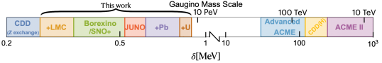
Figure 1: Summary of existing limits and projections on the mass splitting $\delta$ for the Higgsino dark matter scenario for $m_{\tilde{H}}=1.1$ TeV. Existing limits come from tree-level direct detection via Z-exchange [6, 7] in dark blue for small splitting and ACME II [8] in purple.

The Higgsino arises as a natural DM candidate in the Minimal Supersymmetric Standard Model (MSSM) or more generic models of low-scale supersymmetry. The Higgsino as a DM candidate has been well studied [9]. We provide a succinct summary of the important parameters here.

The Higgsino has Dirac mass $\mu\tilde{H}_{u}\tilde{H}_{d}$ before electroweak symmetry breaking (EWSB), which leads to a neutral Dirac fermion and a charged Dirac fermion with identical masses. However, EWSB results in a Majorana mass $m_{M}\approx m_{Z}^{2}\left(\frac{\sin^{2}\theta_{W}}{M_{1}}+\frac{\cos^{2}\theta_{W}}{M_{2}}\right)$, where $m_{Z}$, $M_{1}$, and $M_{2}$ are the masses of the Z boson, the bino, and the wino, respectively. In the limit where the gauginos are much heavier than the Z boson, the Majorana mass is small compared to the Dirac mass $\mu$, resulting in pseudo-Dirac Higgsinos —i.e., two neutral Majorana Higgsinos $\tilde{H}_{1}$ and $\tilde{H}_{2}$ that are almost degenerate. Their individual masses are $M_{\tilde{H}_{1,2}}\approx\mu\mp\frac{\delta}{2}$ with $\delta=m_{M}$, the Majorana mass generated after EWSB. Therefore, the mass splitting is given by

$$\delta\approx m_{Z}^{2}\left(\frac{\sin^{2}\theta_{W}}{M_{1}}+\frac{\cos^{2}\theta_{W}}{M_{2}}\right)~{}.$$ (1)

Particularly compelling is the Higgsino mass $\mu\approx 1.1~{}\textrm{TeV}$, as this would produce the correct relic abundance observed today via freeze-out. The lifetime of the heavier Higgsino $\tilde{H}_{2}$ is typically much shorter than the age of the universe, so the lighter state $\tilde{H}_{1}$ constitutes all of dark matter today. Whenever there is no ambiguity, we will denote the lighter Higgsino state by $\tilde{H}$ and its mass by $m_{\tilde{H}}$.

The $1.1$ TeV Higgsino mass is well above the existing limits set by colliders [10]. There are promising prospects for its indirect detection [11, 12] at CTA [13]. However this critically depends on the amount of dark matter at the galactic center which is uncertain. We explore a complementary direction in this work: its direct detection on earth.

The Higgsino splitting after EWSB results in a purely off-diagonal coupling of the Z boson to the Higgsino mass eigenstates. While the splitting is negligible at freeze-out scales, it becomes crucial for direct detection today. The Z mediator produces a per-nucleon cross section for direct detection

$$\sigma_{\tilde{H}n}\approx 10^{-39}\textrm{cm}^{2}~{}.$$ (2)

Despite being a large cross section for direct detection purposes, this process is inelastic in nature, as the lighter $\tilde{H}_{1}$ needs to up-convert to $\tilde{H}_{2}$. This can only occur if there is enough energy in the center-of-momentum frame. The largest splitting we can probe in collisional direct detection (CDD), $\delta_{\rm CDD}$, is given by

$$\delta_{\rm CDD}=\frac{1}{2}\mu_{A}v_{\rm max}^{2}~{},$$ (3)

where $\mu_{A}\approx m_{A}$ is the reduced mass of the target nucleus with mass $m_{A}$ (and nuclear mass number $A$) that is scattering with the Higgsino $\tilde{H}$, and $v_{\rm max}$ is the maximum DM velocity locally. Since $\frac{1}{2}\mu_{A}v_{\text{max}}^{2}\approx 200~{}\textrm{keV}$ for a typical collisional direct detection nucleus and the Milky Way DM population, this sets the maximum splitting above which there are no current limits on the Higgsino. This falls just short of the $\delta\gtrsim 200$ keV ($\delta\gtrsim 1~{}$ MeV) for small (large) $\tan\beta$ motivated by fine-tuning arguments [9].

Figure 1 provides a rough summary of existing and future coverage for the splitting $\delta$ for $m_{\tilde{H}}$=$1.1$ TeV. We also show for reference the approximate gaugino mass derived from eq. (1) on the top axis. Existing limits from CDD found in literature that go up to roughly $260$ keV [6, 7] are shown in blue and marked “CDD (Z exchange).”

Direct detection could also occur via elastic processes such as Higgs exchange or via one-loop. The Higgsino-Higgs coupling arises via its mixing with gauginos. As a result, the Higgs exchange cross section is dominant when the gaugino mass is close to the Higgsino mass and decouples with the gaugino mass. Current limits on the Higgs exchange rule out Higgsinos only if the gauginos are also at the TeV scale [9], which in turn constrains mass splittings of $\delta\approx 1~{}\textrm{GeV}$ or larger. The projected reach for the LZ experiment corresponds to 10-TeV gauginos, which in turn translates to splittings of $\delta\approx 100~{}\textrm{MeV}$. This is shown as “CDD (H)” in yellow in Figure 1. The loop cross section has an accidental cancellation between different contributions, resulting in it being within the neutrino fog.

A powerful probe of a TeV-scale Higgsino that does not depend on its relic abundance is the measurement of the electric dipole moment (EDM) of the electron. CP violation is generically large in SUSY extensions of the Standard Model. As a result, charginos and neutralinos together induce an EDM on the electron. Once again, these vanish when the gaugino masses are very large. Currently, the EDM limits from ACME II [8, 14], which constrain the EDM to $d_{e}<1.1\times 10^{-29}~{}\textrm{e~{}cm}$, rule out 10 TeV or heavier gauginos for $\tan\beta=2$, with limits degrading for larger $\tan\beta$. This corresponds to $\delta\approx 200~{}\text{MeV}$ Higgsino splitting. Projections from Advanced ACME, with sensitivity to $d_{e}\lesssim 10^{-30}\textrm{e~{}cm}$, corresponds to $100~{}\textrm{TeV}$ gauginos for $\tan\beta=2$, which can probe splittings down to 30 MeV. These are shown as the purple and blue blocks appropriately labeled in Figure 1. The reach will be much weaker for larger $\tan\beta$.

To summarize, the Higgsino splitting $\delta$, the only unknown parameter in the theory, is currently constrained from above at the 100 MeV – GeV scale from EDM limits and Higgs exchange direct detection cross sections. While these constraints are expected to improve, even in the most optimistic scenarios, future experiments are not expected to probe below $30~{}\textrm{MeV}$ splitting.

This challenging window between $200~{}\textrm{keV}$ and $30~{}\textrm{MeV}$ has a remarkable property that might make new ideas for direct detection feasible. Suppose there is a process that successfully scatters $\tilde{H}_{1}$ to $\tilde{H}_{2}$. The $\tilde{H}_{2}$ is unstable, and for small enough mass splitting ($\delta<1~{}\textrm{GeV}$), its dominant decay is to a $\tilde{H}_{1}$ and a photon. This process occurs radiatively via a W loop, and the resultant decay length for a Higgsino with typical DM velocity is given by [15]

$$l_{\tilde{H}_{2}}=7.46~{}\text{km}\left(\frac{v}{400~{}\text{km}/\text{s}}\right)\left(\frac{400~{}\text{keV}}{\delta}\right)^{3}~{},$$ (4)

i.e., the mass splitting window that evades even optimistic projections from other methods corresponds to decay lengths well within terrestrial reach. This opens up a “luminous dark matter” direct detection prospect: if we can find a way to up-convert from the ground state to the excited state, we can observe the subsequent decay to a photon, which will produce a line signal.

How do we increase sensitivity to larger splitting? The answer to this question is captured in eq. (3). The existing limit is set by the heavy nuclei involved (typically Xe) and the maximum velocity of DM particles, currently assumed to follow the Standard Halo Model (SHM). Furthermore, as summarized in previous work [16], the existing limits do not reach the estimate in eq. (3) because inelastic scattering favors larger energy recoils, which are outside the low-background region targeted by existing experiments.

This work hinges on three key observations as applied to the luminous dark matter method. First, in the luminous DM process, the entire energy available in the center-of-momentum frame can be used to upscatter dark matter, unlike in collisional direct detection, where some energy has to go to the nuclear recoil to make it detectable. Second, in the luminous DM method, the nuclei act merely as springboards to up-scatter dark matter and are not involved in the detection itself. Therefore, heavy nuclei like Pb, or even U and Th, can be used, maximizing the reduced mass and thereby increasing sensitivity to the mass splitting. Finally, recent work has pointed to a dark matter sub-population with origins in the LMC that populates the high-velocity tail of dark matter, exceeding the MW escape velocity. These points are explored in detail in the rest of the paper and correspond to the improvements seen in Figure 1 labeled “this work.”

III Luminous Detection

In this section, we describe the process of luminous detection using large-volume neutrino detectors and calculate the expected signal rate based on a homogeneous approximation of the Earth.

In this paper, we use the term “direct detection” to refer to any experiment that seeks to interact directly with relic DM particles. Within the broad category of direct detection, we use the term “collisional direct detection (CDD)” to refer to traditional WIMP detectors that search for nuclear recoils and “luminous detection” for searches for their luminous signals.

III.1 Terrestrial Scattering and Large-Volume Detectors

The typical Higgsino decay length $l_{\tilde{H}_{2}}$ (eq. (4)), which is on the order of a few kilometers, is much larger than the size of any detector but much smaller than the Earth’s radius: $R_{D}\ll l_{\tilde{H}_{2}}\ll\mathrm{R}_{\mathTerra}$. This hierarchy enables the luminous DM detection process:

1. A Higgsino DM particle $\tilde{H}_{1}$ upscatters with a heavy nucleus in the Earth;

2. The excited state $\tilde{H}_{2}$ subsequently travels a distance of $\sim l_{\tilde{H}_{2}}$ before decaying in a detector into $\tilde{H}_{1}$ and a photon.

The resulting DM signature would be a monoenergetic line of frequency $\delta$. Note that this process is not exclusive to Higgsinos, but applies to any inelastic DM model with a decay length that satisfies the aforementioned hierarchy. This mechanism was first explored in Ref. [3] in the context of explaining the DAMA signal.

Despite the dual requirements that the excited particle must travel in the direction of the detector and decay within the detector, these geometrical constraints are precisely compensated by the large volume of the surrounding Earth. In fact, if the detector is located deep within the Earth, the Earth can be approximated as having infinite extent and homogeneous density, in which case the upscatterings and decays clearly form an equilibrium, occurring at the same rate within a given volume. Consequently, the luminous DM signal rate is roughly the same as the rate for direct collisions within the detector volume and is independent of the decay length. In fact, the rate depends solely on the detector volume and scales linearly with it. We will demonstrate this explicitly by calculating the signal rate using the homogeneous Earth approximation below.

Since the luminous signal scales with detector volume, a large-volume detector sensitive to photons in the hundreds of keV range is ideal. Ref. [4] noted that the underground neutrino detector Borexino [17], with a scintillator radius of $4.25$ meters and a threshold of $E_{\text{thr}}=150$ keV, is well-suited for this purpose. By treating both the radioactivity of the surrounding and the observed solar neutrinos as background, Ref. [4] showed that an analysis of Borexino’s existing data, looking for a daily modulation signal, can already set new limits on Higgsino DM. They also pointed out that the under-construction neutrino detector JUNO [18], with a radius of $17.5$ meters, has the potential to set even stronger limits in the future.

We will describe several improvements on Ref. [4] in later sections. Among other things, we will demonstrate that performing a line search instead of or in addition to a daily modulation search (see Section VI.3) offers advantages. Additionally, we show that the SNO+ experiment [19], which has a radius of $6$ meters, can be added to the roster of large-volume neutrino detectors (see Table 3) with exciting potential for Higgsino discovery, despite its high latitude. Before discussing these and other new results, we first lay out the formalism used to compute the luminous DM signal rate.

III.2 Signal Rate Calculation

In the homogeneous Earth approximation, the detector is situated deep within the Earth, which is modeled as having infinite extent and uniform density. Consider a single element with nuclear mass number $A$ present in the Earth; we will denote the nucleus or element by $A$. If a single nucleus has a Higgsino-nucleus scattering rate $\Gamma_{\tilde{H}A}$, then the total photon signal rate $\Gamma_{\gamma}$ can be obtained by multiplying the effective number of nuclei in the Earth that can produce photon signals

$$\Gamma_{\gamma}=\Gamma_{\tilde{H}A}n_{A}V_{\text{eff}}~{},$$ (5)

where $n_{A}$ is the number density of element $A$ in the Earth, and $V_{\text{eff}}$ is the effective volume that we now estimate.

To calculate the effective volume, let the center of the detector with radius $R_{D}$ be at the origin of our coordinate system. A $\tilde{H}$–$A$ scattering occurs outside the detector at position $\mathbf{r}$ (with $r>R_{D}$), where a $\tilde{H}_{1}$ upscatters into a $\tilde{H}_{2}$. The fractional flux in the direction of the detector is determined by the fraction of the surface area of the spherical shell of radius $r$ centered at $\mathbf{r}$ that is covered by the detector, specifically $\left(\dfrac{R_{D}}{r}\right)^{2}$. Since the decay length $l_{\tilde{H}_{2}}$ is much larger than $R_{D}$, we can approximate the Poisson distribution linearly and apply a suppression factor of $\dfrac{R_{D}}{l_{\tilde{H}_{2}}}$. Integrating up to a radius $l_{\tilde{H}_{2}}$, beyond which the incoming $\tilde{H}_{2}$ begins to significantly decay, the effective volume of the Earth that can produce a signal is approximately

$$V_{\text{eff}} \approx 4\pi\int_{R_{D}}^{l_{\tilde{H}_{2}}}dr~{}r^{2}\left(\dfrac{R_{D}}{r}\right)^{2}\dfrac{R_{D}}{l_{\tilde{H}_{2}}}$$ (6)

$$\approx 3\left(\frac{4\pi}{3}R_{D}^{3}\right)$$ (7)

$$=3V_{D}~{}.$$ (8)

Notice that all the length scales cancel out, resulting in a trivial integral and an effective volume three times the detector volume. Notably, the signal is proportional to the detector volume.

The scattering rate $\Gamma_{\tilde{H}A}$ is related to the Higgsino-nucleus cross section $\sigma_{\tilde{H}A}$ by

$$\frac{d\Gamma_{\tilde{H}A}}{dE_{R}}=n_{\tilde{H}}\int_{v>v_{\text{min}}(E_{R})}d^{3}v~{}\frac{d\sigma_{\tilde{H}A}}{dE_{R}}~{}v~{}f^{\text{det}}(\mathbf{v})~{},$$ (9)

where $n_{\tilde{H}}$ is the DM number density, $E_{R}$ is the nuclear recoil energy, and $v$ is the DM velocity in Earth’s frame. The function $f^{\text{det}}(\mathbf{v})$ represents the time-averaged DM velocity distribution in the detector’s frame. Since the experiment runs over many years, we take this time average. Although this procedure preserves the maximum velocity $v_{\text{max}}$, it neglects the yearly modulation of the signal, a useful experimental handle [4].

The term $v_{\text{min}}(E_{R})$ is the minimum velocity required to produce a given recoil energy $E_{R}$ and mass splitting $\delta$. In the limits $\delta\ll m_{\tilde{H}}$, it is given by [20]

$$v_{\text{min}}(E_{R})=\frac{1}{\sqrt{2m_{A}E_{R}}}\left(\frac{m_{A}}{\mu_{A}}E_{R}+\delta\right)~{},$$ (10)

where $\mu_{A}$ is the reduced mass relative to the nucleus and $m_{A}$ is the nucleus mass. Although $v_{\text{min}}(E_{R})$ depends on the recoil energy, there is also a global minimum velocity $v_{\text{min,global}}$, which is the minimum velocity required for any upscattering to occur. It is given by

$$v_{\text{min,global}}=\sqrt{\frac{2\delta}{\mu_{A}}}~{}.$$ (11)

For a spin-independent interaction, the differential cross section is related to the total cross section $\sigma_{\tilde{H}A}$ by

$$\frac{d\sigma_{\tilde{H}A}}{dE_{R}}=\frac{m_{A}\sigma_{\tilde{H}A}}{2\mu_{A}^{2}v^{2}}~{}.$$ (12)

Due to the coherent scattering of $\tilde{H}$ with the entire nucleus, $\sigma_{\tilde{H}A}$ is related to the Higgsino-nucleon cross section $\sigma_{\tilde{H}n}$ by [21]

$$\sigma_{\tilde{H}A}=A^{2}\left(\frac{\mu_{A}}{\mu_{n}}\right)^{2}\sigma_{\tilde{H}n}~{}F_{A}^{2}(E_{R})\approx A^{4}\sigma_{\tilde{H}n}~{}F_{A}^{2}(E_{R})~{},$$ (13)

where $\mu_{n}\approx m_{n}\approx 1$ GeV is the reduced mass relative to a single nucleon. The breakdown of coherence is accounted for by the inclusion of the Helm form factor, which is given by [4]

$$F_{A}(E_{R})=\frac{3}{qr_{n}}J_{1}(qr_{n})e^{-q^{2}s^{2}/2}~{},$$ (14)

where $J_{1}(x)$ is a spherical Bessel function, $q=\sqrt{2m_{A}E_{R}}$ is the momentum transfer, $s\approx 0.9$ fm, and $r_{n}\approx 1.14\left(\dfrac{A}{0.93}\right)^{1/3}$ fm. Combining these results, the differential scattering rate becomes

$$\frac{d\Gamma_{\tilde{H}A}}{dE_{R}} =n_{\tilde{H}}\frac{m_{A}A^{4}\sigma_{\tilde{H}n}}{2\mu_{A}^{2}}~{}\eta(v_{\text{min}}(E_{R}))~{}F_{A}^{2}(E_{R})~{},$$ (15)

where the mean inverse velocity, or halo integral $\eta$ (see Sec IV.2) [22], is treated as a function of $E_{R}$:

$$\eta(v_{\text{min}}(E_{R}))\equiv\int_{v>v_{\text{min}}(E_{R})}d^{3}v~{}\frac{1}{v}f^{\text{det}}(\mathbf{v})~{}.$$ (16)

Integrating over all nuclear recoil energies $E_{R}$, summing over all relevant elements in the Earth, and relating $\sigma_{\tilde{H}n}$ back to the observable $\Gamma_{\gamma}$, we obtain

$$\Gamma_{\gamma} =\sigma_{\tilde{H}n}\times V_{\text{eff}}~{}n_{\tilde{H}}\sum_{A}n_{A}\frac{m_{A}A^{4}}{2\mu_{A}^{2}}\int_{0}^{\infty}dE_{R}~{}\eta(v_{\text{min}}(E_{R}))~{}F_{A}^{2}(E_{R})~{}.$$ (17)

The DM number density is given by $n_{\tilde{H}}=\rho_{\rm DM}/m_{\tilde{H}}$, where we take $\rho_{\rm DM}=0.3~{}\text{GeV}/\text{cm}^{3}$. We show how to use this equation to set 90% confidence level limits in Section VI.3.2.

Even though $\sigma_{\tilde{H}n}=10^{-39}\textrm{cm}^{2}$ is fixed for the Higgsino, this equation applies to any inelastic dark matter with the same mass, $m_{\tilde{H}}=1.1$ TeV, and a decay length $l_{\text{DM}}$ satisfying $R_{D}\ll l_{\text{DM}}\ll\mathrm{R}_{\mathTerra}$. Therefore, we will use the notation $\sigma_{\text{DM},n}$ for the general case. Note that when we consider adding supplemental Pb/U near the detector in Section VI.1, the signal rate will depend on the decay length, and those equations will only generalize to models with the same mass and decay length as the Higgsino.

It is important to note that this homogeneous Earth approximation neglects the directionality of the fastest DM population, which is particularly relevant for large mass splittings $\delta$. Within the SHM, the fact that the Sun moves through the MW implies that the fastest dark matter originates from the direction of the constellation Cygnus [23, 4]. The effects of the LMC result in faster DM particles, but they share a similar directionality (see Section IV.1). This directionality induces a daily modulation in the luminous DM signal because, during the part of the sidereal day when Cygnus has risen above the Earth’s horizon at the location of the detector, there may not be sufficient Earth volume for the Higgsino to scatter with on its way to the detector. Furthermore, since the Higgsino is much heavier than any nucleus, after scattering, it continues to move forward in Earth’s frame, with a small deflection angle of at most $\sim 10^{\circ}$ [4]. This forward scattering preserves the directionality of the DM signal.

The primary impact of the inhomogeneity on our results is that the signal is suppressed for roughly half of each sidereal day, resulting in a signal time that is only half of the total runtime:

$$t_{\text{signal}}=t_{\text{total}}/2~{}.$$ (18)

We explore this topic further in Section VI.3. Nevertheless, aside from this adjustment, the effects of inhomogeneity average out, making the signal rate in the homogeneous approximation a reliable estimate. Moreover, the detector’s proximity to Earth’s surface does not lead to an overestimation of the signal, as the flux is predominantly unidirectional in reality.

IV Dark Matter Populations

In this section, we introduce two halo models, the SHM and the LMC model. We also calculate the existing limits on inelastic DM from collisional direct detection using both halo models.

IV.1 Dark Matter from the Large Magellanic Cloud

Ref. [4] treats the velocity distribution of dark matter using the SHM [24], which, in the galactic frame, is given by a truncated Maxwell-Boltzmann distribution

$$f^{\text{gal}}_{\text{SHM}}(\mathbf{v})~{}\propto~{}\exp\left(-\frac{v^{2}}{v_{0}^{2}}\right)\Theta(v_{\text{esc}}-v)~{},$$ (19)

where $v_{0}=220~{}\text{km}/\text{s}$ is the local standard of rest, $v_{\text{esc}}=540~{}\text{km}/\text{s}$ is the escape velocity of the MW, and $\Theta$ is the Heaviside step function. We have used the astrophysical parameters from Ref. [22]. We will take this SHM as one of our two example halo models. The SHM is the default model used in most analyses of direct detection experiments due to its simplicity and its natural explanation of flat rotation curves [25, 26], despite its many known inaccuracies [27, 28, 29, 30, 31]. However, the SHM is a poor approximation in the context of inelastic dark matter. Probing large mass splittings requires high DM velocities, but the high-velocity tail of the distribution is particularly sensitive to halo merger history [25, 30].

Recent studies [32, 22, 33] argue that the high-velocity tail of the local dark matter distribution predominantly originates from the LMC and includes particles moving faster than the escape velocity of the MW. The LMC is a massive satellite galaxy that recently made its first close approach to the MW $\sim 50$ Myr ago [34]. This encounter left behind two high-speed DM populations in the solar neighborhood: particles originating from the LMC and MW particles that were accelerated by the LMC’s gravitational force. Since these two populations have roughly the same phenomenology, we will not distinguish between them and will collectively refer to them as “dark matter from the LMC.”

The effects of the LMC are prominent due to several factors. First, it has a large infall mass, approximately $10\%$ that of the MW, thereby exerting a strong gravitational influence. Second, it only recently passed through the MW for the first time, so its particles have yet to equilibrate and can retain high velocities. Most importantly, the LMC happens to be moving in the opposite direction to the Sun [32], leading to large relative velocities between the dark matter from the LMC and the Earth. This is a fortunate coincidence—had we lived on the other side of the galactic disc, the relative velocities would have been lower by $\sim 240~{}\text{km}/\text{s}$ [32].

The fact that the dark matter from the LMC is moving in the opposite direction from the Sun also has important implications for the daily modulation of the signal. In the SHM, the fastest dark matter comes from the direction of the Sun’s motion with respect to the galaxy, which coincides with the direction of the constellation Cygnus [23]. The proposal in Ref. [4] relies on the fact that Cygnus is above the horizon for only part of the sidereal day for detectors at suitable latitudes, leading to a daily modulation in the signal. Since dark matter from the LMC also appears to originate from the direction of Cygnus, it would produce the same daily modulation signal. However, as we argue in Section VI.3, daily modulation is not essential for detecting a signal since we can perform a line search instead. Nevertheless, the daily modulation must be properly accounted for in our analysis and could also be a useful part of a real experimental analysis.

Ref. [22] studies the LMC’s effects using cosmological simulations that account for the formation history of the MW and the LMC. That paper utilized the Auriga cosmological magneto-hydrodynamical simulations [35] and focused on a particular MW analogue, referred to as halo 13 (Auriga ID Au-25), which has an LMC analogue. The simulation was rerun with finer time resolution, and its present-day DM velocity distribution was computed. Table 1 shows that the MW’s virial mass, local dark matter density, the LMC’s infall mass, relative velocity at closest approach (pericenter), and present-day relative distance and velocity in the simulation are compatible with observed values. Although the distance and time of the closest approach deviate somewhat from the observed values, these parameters are realistic enough to be considered a reasonable proxy for the real MW-LMC system and were therefore used to analyze the results of direct detection experiments in that paper. We follow Ref. [22] in using the velocity distribution from this simulation (henceforth, the LMC model), acknowledging that it is not a perfect match to the real MW-LMC system. Future simulations may yield an even closer match. As we shall see, incorporating the effects of the LMC significantly boosts our sensitivity to Higgsinos and inelastic DM more generally.

	$M^{\text{MW}}_{\text{vir}}~{}[10^{11}\mathrm{M}_{\mathSun}]$	$\rho_{\rm DM}~{}[\text{GeV}/\text{cm}^{3}]$	$M^{\text{LMC}}_{\text{Infall}}~{}[10^{11}\mathrm{M}_{\mathSun}]$	$r_{\text{peri}}~{}[\text{kpc}]$	$v_{\text{peri}}~{}[\text{km}/\text{s}]$	$t_{\text{peri}}~{}[\text{Myr}]$	$r_{\text{pres}}~{}[\text{kpc}]$	$v_{\text{pres}}~{}[\text{km}/\text{s}]$
observed	10–20	$\sim 0.3$	$\sim$ 1–3	$\sim 48$	$340\pm 19$	$\sim-50$	$\sim 50$	$321\pm 24$
simulation	12	0.34	3.2	32.9	$[205,376]$	-133	50.6	317

Table 1: Comparison of the properties of the MW and LMC with their simulated analogues, referred to as halo 13 in Ref. [22]. $M^{\text{MW}}_{\text{vir}}$ is the virial mass of the MW [36]. $\rho_{\rm DM}$ is the local dark matter density [37]. $M^{\text{LMC}}_{\text{Infall}}$ is the virial mass of LMC at infall. $r_{\text{peri}}$ and $v_{\text{peri}}$ are the distance [32] and velocity [38], respectively, between the MW and LMC at closest approach (pericenter). $t_{\text{peri}}$ is the time of pericenter relative to the present day ($t=0$), and $r_{\text{pres}}$ and $v_{\text{pres}}$ are the present-day values.

IV.2 Halo Integrals

A direct detection experiment’s sensitivity to dark matter typically depends on the velocity distribution only indirectly, through the halo integral, which we now introduce, following Ref. [22]. Let $f^{\text{gal}}(\mathbf{v})$ denote the present-day DM velocity distribution in the galactic frame. We transform this to the detector reference frame as

$$f^{\text{det}}(\mathbf{v},t)=f^{\text{gal}}(\mathbf{v}+\mathbf{v}_{\mathTerra}(t)+\mathbf{v}_{\mathSun})~{},$$ (20)

where $\mathbf{v}$ is the DM velocity in Earth’s frame; $\mathbf{v}_{\mathTerra}(t)$ is Earth’s velocity relative to the Sun, which varies over the course of a year; and $\mathbf{v}_{\mathSun}$ is the Sun’s velocity relative to the galactic frame. For a given minimum DM lab-frame velocity $v_{\text{min}}$ (see eq. (10)), the mean inverse velocity above $v_{\text{min}}$ is known as the halo integral [22],

$$\eta(v_{\text{min}},t)\equiv\int_{v>v_{\text{min}}}d^{3}v~{}\frac{1}{v}f^{\text{det}}(\mathbf{v},t)~{},$$ (21)

as introduced in eq. (16). We then take its time average,

$$\eta(v_{\text{min}})\equiv\langle\eta(v_{\text{min}},t)\rangle~{}.$$ (22)

We extract $\eta(v_{\text{min}})$ for the LMC model from Ref. [22], which is reproduced in Figure 2, along with that of the SHM for comparison. Since the SHM is truncated at the MW escape velocity $v^{\rm gal}_{\rm esc}=540~{}\text{km}/\text{s}$ in the galactic frame, this corresponds to a cutoff of $v^{\text{SHM}}_{\text{max}}=760~{}\text{km}/\text{s}$ in the detector frame. However, once the dark matter from the LMC is considered, the maximum DM velocity increases significantly to $v^{\text{LMC}}_{\text{max}}=950~{}\text{km}/\text{s}$.

Figure 2: Time-averaged halo integrals of the SHM compared to the LMC model. The SHM is truncated at the MW escape velocity, $v^{\text{SHM}}_{\text{max}}=760~{}\text{km}/\text{s}$, in the detector frame, while the LMC model reaches a higher maximum velocity $v^{\text{LMC}}_{\text{max}}=950~{}\text{km}/\text{s}$. Figure adapted from Ref. [22].

IV.3 Existing Limits on Inelastic Dark Matter

Traditional WIMP detectors can detect inelastic dark matter scattering by measuring the nuclear recoil of the target nuclei, a process we refer to as collisional direct detection. As a new result of this paper, we calculate updated bounds on inelastic dark matter from collisional direct detection using both the SHM and the LMC model. Note that the mechanism of direct collisions with target nuclei is not specific to the Higgsino model, so the result is applicable to any inelastic dark matter with mass $m_{\tilde{H}}=1.1$ TeV. However, the intersection of a constraint curve with the $\sigma_{\text{DM},n}=10^{-39}~{}\text{cm}^{2}$ line delineates the corresponding limit on the Higgsino.

The collision event rate $\Gamma_{c}$ of a traditional WIMP detector is given by

$$\Gamma_{c} =\sigma_{\text{DM},n}\times N_{A}~{}n_{\text{DM}}\frac{m_{A}A^{4}}{2\mu_{A}^{2}}\int_{0}^{\infty}dE_{R}~{}\varepsilon(E_{R})~{}\eta(v_{\text{min}}(E_{R}))~{}F_{A}^{2}(E_{R})~{},$$ (23)

where $A$ is the nuclear mass number of the target nuclei (e.g., Xe or iodine (I)), $N_{A}$ is the number of target nuclei in the detector, $n_{\text{DM}}$ is the DM number density, and $\varepsilon(E_{R})$ is the detection efficiency of the experiment. We use the halo integrals for the SHM and the LMC model found in Ref. [22], reproduced in Figure 2.

The results are shown in Figure 3. The most stringent current limit on Higgsino is set by PandaX-4T [6], with $\delta^{\text{SHM}}_{\text{PandaX}}\sim 260$ keV and $\delta^{\text{LMC}}_{\text{PandaX}}\sim 340$ keV. These limits are also shown in Figure 1 as “CDD (Z exchange)” in blue and “+LMC” in orange, respectively. PICO-60 $\text{CF}_{3}\text{I}$ [7] exhibits better sensitivity at higher $\delta$, but not for the Higgsino. Compared to other WIMP experiments, these two experiments benefit from higher efficiencies at large recoil energies.

Some WIMP experiments have collected high recoil-energy data but excluded them from their analyses, resulting in low efficiencies at high recoil energy and inadvertently limiting their sensitivities to inelastic DM at high $\delta$. As recommended in previous works [16], we advocate reanalyzing existing data over a larger range of recoil energy, as this presents an easy opportunity to improve current inelastic DM bounds.

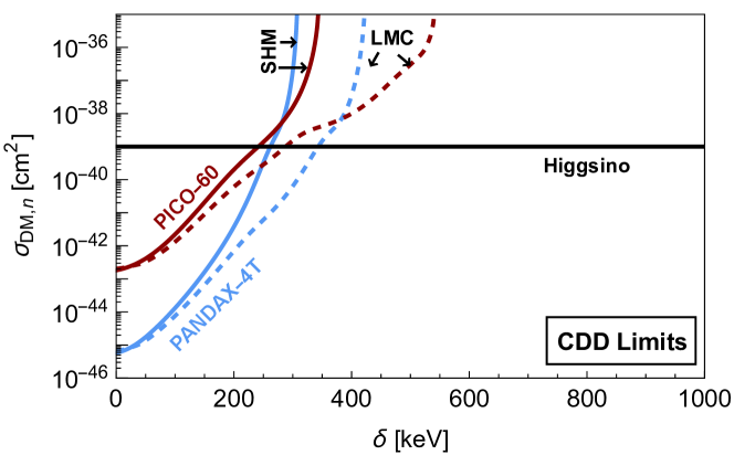
Figure 3: Our estimates for the current limits on inelastic dark matter from collisional direct detection (CDD), based on the PandaX-4T [6] and PICO-60 $\text{CF}_{3}\text{I}$ [7] experiments, are shown via the DM-nucleon cross section $\sigma_{\text{DM},n}$ vs splitting $\delta$. The limits are shown for our two example halo models, the SHM and the LMC model. The horizontal line shows the cross section for the standard Higgsino DM candidate. These limits, derived from direct scattering inside the detectors, apply to any inelastic dark matter candidate—not just the Higgsino—provided the decay back to the ground state occurs outside the detector.

V Terrestrial Heavy Elements

The maximum $\delta$ that can be upscattered by the element $A$ is determined using eq. (11),

$$\delta_{\text{max},A}=\frac{1}{2}\mu_{A}v_{\text{max}}^{2}\approx\frac{1}{2}Am_{n}v_{\text{max}}^{2}~{},$$ (24)

where $m_{n}\approx 1$ GeV is the nucleon mass, and $v_{\text{max}}$ is the maximum lab-frame DM velocity. In our two halo models, $v^{\text{SHM}}_{\text{max}}=760~{}\text{km}/\text{s}$ and $v^{\text{LMC}}_{\text{max}}=950~{}\text{km}/\text{s}$. Given our limited sensitivity to larger Higgsino mass splittings $\delta$, it becomes essential to account for any heavy elements in the Earth with appreciable abundances. Ref. [4] focused on the trace abundances of Pb ($A=207$).

In this paper, we consider two heavier elements, Th ($A=232$) and U ($A=238$), whose number densities in Earth’s crust are smaller than that of Pb by factors of 2 and 10, respectively; see Table 2. Their lower abundances are partially compensated by the $A^{4}$ scaling in eq. (17), which arises from the coherent scattering of the Higgsino with the entire nucleus [21]. The significance of Th and U is amplified by the much larger $(v^{\text{LMC}}_{\text{max}})^{2}$ term in eq. (24). As shown in Table 2, U can upscatter a maximum mass splitting of $\delta^{\text{LMC}}_{\text{max},\text{U}}\sim 940$ keV, exceeding Pb’s reach by over $100$ keV. Although this 100-keV improvement is most readily applicable to larger cross sections and is not immediately realized on the Higgsino line in the simplest searches (see Figure 4), more aggressive strategies—such as adding U/Pb supplements around the detector, as discussed in Section VI.1—can be employed to lower the constraint curves (see Figures 5 and 6), making Th and U relevant for the Higgsino. Furthermore, beyond the Higgsino, more general inelastic DM models with larger cross sections would more readily benefit from this improvement.

In Table 2, we also show other terrestrial elements considered in addition to the heavy elements Pb, Th, and U. Among the major elements in the mantle, only calcium (Ca) and iron (Fe) can scatter with splittings $\delta^{\text{LMC}}_{\text{max},A}$ above Borexino’s threshold $E_{\text{thr}}=150$ keV. We also include barium (Ba) and strontium (Sr), which have intermediate values of $\delta_{\text{max},A}$ and appreciable abundances in the mantle and crust. Additionally, we list the Higgsino decay lengths at $\delta_{\text{max},A}$ for each element, given by

$$l_{\text{max},A}\equiv l_{\tilde{H}_{2}}(v_{\text{max}},\delta_{\text{max},A})~{},$$ (25)

for both the SHM and LMC model. While this is not the maximum distance over which an element can have an impact—since it can always scatter at lower $\delta$, which would travel farther—it serves as a useful length scale associated with each element. The details of computing number densities and how we incorporate the varying densities in Earth’s crust and mantle are provided in Appendix A.

element	$A$	$n_{A}~{}[\text{km}^{-3}]$	$a_{A}$	relevant source	$\delta^{\text{LMC}}_{\text{max},A}~{}[\text{keV}]$	$l^{\text{LMC}}_{\text{max},A}~{}[\text{km}]$	$\delta^{\text{SHM}}_{\text{max},A}~{}[\text{keV}]$	$l^{\text{SHM}}_{\text{max},A}~{}[\text{km}]$
Ca	40.078	$1.8\times 10^{36}$	0.0261	mantle	$180$	$180$	120	150
Fe	55.85	$3.0\times 10^{36}$	0.063	mantle	$250$	$71$	160	56
Sr	87.62	$6.8\times 10^{32}$	$22\times 10^{-6}$	mantle	$390$	$20$	250	16
		$6.2\times 10^{33}$	$320\times 10^{-6}$	total crust
Ba	137.33	$1.4\times 10^{32}$	$6.85\times 10^{-6}$	mantle	$580$	$5.8$	370	4.6
		$5.7\times 10^{33}$	$456\times 10^{-6}$	total crust
Pb	207.2	$1.4\times 10^{32}$	$17\times 10^{-6}$	upper crust	$830$	$2.0$	530	1.6
Th	232.04	$7.7\times 10^{31}$	$10.5\times 10^{-6}$	upper crust	$920$	$1.5$	580	1.2
U	238.03	$1.9\times 10^{31}$	$2.7\times 10^{-6}$	upper crust	$940$	$1.4$	590	1.1

Table 2: Relevant elements in the Earth. Listed are the nuclear mass number $A$, their number density $n_{A}$, their mass abundances $a_{A}$ in the crust [40] and mantle [41]. We also show the maximum mass splitting each element can scatter and the corresponding decay length for the two example halo models, the SHM and LMC model. See Appendix A for further details.

VI Advanced Luminous Detection Techniques

In this section, we introduce three strategies to enhance luminous detection of Higgsino dark matter. Specifically, in the following three subsections, we propose a method to enhance signals, a preliminary idea to reduce background, and a new analysis approach that make more detectors viable for this purpose.

VI.1 Uranium and Lead Supplements

As previously explained, new limits on Higgsino DM can be set by reanalyzing existing data from Borexino, as well as by performing similar analyses with upcoming detectors such as JUNO and SNO+. The most stringent limit of this type can be achieved by JUNO due to its larger volume. However, as shown in Figure 6(a), although it is kinematically possible for U to excite mass splittings up to $\delta^{\text{LMC}}_{\text{max,U}}\sim 940~{}\text{keV}$, JUNO can only set a limit of $\delta^{\text{LMC}}_{\text{JUNO}}\sim 580$ keV with a 10-year runtime. While this represents a significant improvement over the current limit of $\delta^{\text{LMC}}_{\text{PandaX}}\sim 340$ keV, it still falls short of its kinematic potential. Further sensitivity will be necessary to lower the constraint curves.

To this end, we propose installing a large volume of Pb or U near the detector. This would dramatically increase the number density of the heavy elements compared to their trace abundances in the Earth. Furthermore, the scattering rate with the installed volume does not exhibit daily modulation, effectively doubling its exposure time relative to terrestrial elements. Note that the line search method is required to detect such a signal (see Section VI.3). Another advantage of the Pb/U supplement is its flexibility, as it can be moved or removed to further reduce background or confirm any potential signals, although doing so would forfeit the factor of 2 in exposure time. Acquiring a large volume of either element appears feasible in terms of cost: Pb is relatively inexpensive at $2 USD per kg, and there are $\sim 10^{6}$ tons of depleted U worldwide, with limited use [42].

Although the Pb/U supplement provides a much larger number density $n_{\text{Pb,supp}}\gg n_{\text{pb,Earth}}$ in the signal rate formula eq. (17), the effective volume term $V_{\text{eff}}$, which previously represented the relevant volume of the surrounding Earth, is now replaced by the much smaller effective volume of the Pb/U material. We calculate this modified effective volume below using a toy model. While we refer to Pb for simplicity, the result is identical for U.

In our toy model, we assume the Pb supplement is distributed into a spherical shell with an outer radius $R_{\text{Pb}}$ surrounding the spherical detector with radius $R_{D}$. In practice, the Pb would optimally be placed as close to the detector as possible. The effective volume $V_{\text{eff}}$, calculated in eq. (6), which is now contributed by the Pb supplement rather than the surrounding Earth, is suppressed by the decay length $l_{\tilde{H}_{2}}$:

$$V_{\text{eff,Pb}} \approx 4\pi\int_{R_{D}}^{R_{\text{Pb}}}dr~{}r^{2}\left(\dfrac{R_{D}}{r}\right)^{2}\dfrac{R_{D}}{l_{\tilde{H}_{2}}}$$ (26)

$$=3V_{D}\left(\frac{R_{\text{Pb}}-R_{D}}{l_{\tilde{H}_{2}}}\right)~{}.$$ (27)

We take the velocity-dependence of $l_{\tilde{H}_{2}}$ to be the minimum velocity $v_{\text{min,global}}$ (eq. (11)) required to upscatter against Pb. Expressing the effective volume of Pb in terms of the actual volume of the Pb supplement $V_{\text{Pb}}=\frac{4\pi}{3}(R_{\text{Pb}}^{3}-R_{D}^{3})$, we obtain

$$V_{\text{eff,Pb}} \approx 3V_{D}\left(\frac{1}{l_{\tilde{H}_{2}}}\right)\left[\left(\frac{3}{4\pi}V_{\text{Pb}}+R_{D}^{3}\right)^{1/3}-R_{D}\right]~{}.$$ (28)

If $V_{\text{Pb}}$ is much smaller than the detector volume, the effective volume increases proportionally with $V_{\text{Pb}}$,

$$V_{\text{eff,Pb}}\approx 3V_{D}\times\frac{1}{4\pi}\frac{V_{\text{Pb}}}{l_{\tilde{H}_{2}}R_{D}^{2}}~{}.$$ (29)

However, once $V_{\text{Pb}}$ becomes much larger than the detector volume, the effective volume increases only linearly with $R_{\text{Pb}}$. Therefore, it is most cost-effective to install a Pb/U supplement with a volume comparable to the detector volume. Since JUNO has a larger volume than SNO+, it continues to benefit for longer as more Pb/U is added.

Another important insight from eq. (28) is that since the decay length $l_{\tilde{H}_{2}}$ is inversely proportional to $\delta^{3}$ (eq. (4)), there is much more severe decay length suppression at low $\delta$, which improves rapidly as $\delta$ increases. At sufficiently low $\delta$, the Pb/U supplement would provide little to no advantage. Fortunately, as shown in Figures 5(a) and 6(a), the Higgsino line crosses the constraint curves at a $\delta$ that benefits significantly from the Pb/U supplement for both SNO+ and JUNO.

VI.2 Towards Background-Free Detection

Aside from being limited by their volumes, the primary obstacle preventing the neutrino detectors from achieving better sensitivity is background, which we have defined as including both the radioactivity of the surroundings as well as observed solar neutrinos. While it is possible to distinguish solar neutrinos by filtering out signals originating from the direction of the Sun, reducing background from radioactivity is much more difficult due to irreducible radioactive impurities. Ref. [4] considered the sensitivity of gaseous scintillation detectors such as CYGNUS [43], which experience less background than liquid scintillators due to their lower density. However, CYGNUS is only sensitive to lower values of $\delta$, whereas our focus is on higher $\delta$ for the Higgsino.

Here, we discuss a preliminary idea for a dedicated, background-free gamma-ray detector for Higgsino DM. Since the standard luminous detection scheme at JUNO can already probe up to $\sim 600$ keV (see Figure 6(a)), we focus on the backgrounds above this energy. Assuming complete rejection of the solar neutrino background is achievable, the remaining backgrounds between $600$ keV and $1$ MeV arise from $\beta$-decays of ${}^{210}\text{Bi}$, ${}^{85}\text{Kr}$, ${}^{40}\text{K}$, and ${}^{11}\text{C}$, as well as $\alpha$-decays of ${}^{238}\text{U}$ and ${}^{232}\text{Th}$ (see Figure 1.10 of Ref. [18]). Crucially, all of these backgrounds are generated by charged particles, while our signal is produced by photons. Therefore, complete background rejection may be possible if we can reliably distinguish between photons and charged particles.

Despite the challenge of achieving this below a few MeV due to the unavailability of pair production, there have been proposals for detectors of this kind in an astrophysics context, such as ASTROGAM, whose Anticoincidence detector has a projected background rejection efficiency of over $99.99\%$ [44]. While complete elimination of backgrounds may never be fully achievable in practice, we present background-free projections in Figure 6 as an ultimate limit for such a dedicated detector.

We are primarily considering the background-free detector as an alternative to the simpler but potentially more costly approach of adding a Pb/U supplement, which also targets the same energy range. It is also possible to combine these two ideas, which will be briefly discussed in Section VII.

VI.3 Line Searches and Detector Depths

VI.3.1 Cygnus and Daily Modulation

As mentioned previously, due to the Sun’s motion relative to the galaxy, most DM particles, especially the high-speed ones, appear to originate from the direction of the constellation Cygnus in Earth’s frame [23, 4]. This effect is well-known within the SHM and remains valid even after accounting for the effects of the LMC, as explained in Section IV.1. Moreover, since the Higgsino is much heavier than any target nucleus, the excited Higgsino continues to travel forward after upscattering, with a small deflection angle of at most $\sim 10^{\circ}$, allowing the luminous signal to retain its Cygnus-directionality [4].

Since Cygnus has a declination of $45^{\circ}$ North, detectors with latitudes above $45^{\circ}$ North always see Cygnus above the horizon, while for detectors below $45^{\circ}$ South, Cygnus is always below the horizon. Detectors located in the intermediate region between these two latitudes see Cygnus above the horizon only for some fractions of the day. Ref. [4] argues that only detectors in this intermediate region can be used to search for inelastic DM effectively for the following reason: while the high-speed DM particle has to pass through the bulk of the Earth to reach the detector when Cygnus is below the horizon, it passes through a much smaller fraction of the Earth when Cygnus is above the horizon. This significantly reduces its signal since there are fewer materials to scatter with, introducing a sidereal daily modulation to the signal. A limit can then be set by requiring that the signal when Cygnus is below the horizon is no larger than the statistical fluctuation of the background, predicted by the measured values when Cygnus is above the horizon.

We note two important additional considerations. First, in addition to a daily modulation search, a line search could also be considered. This approach makes potential detectors located below $45^{\circ}$ South viable candidates. Second, for detectors located above $45^{\circ}$ North, the depths of their underground locations should be carefully considered. Upon accounting for this, certain detectors, notably SNO+, become viable for Higgsino dark matter detection. We demonstrate these two points in the following subsections.

VI.3.2 Line Searches and High Southern Latitudes

While daily modulation is an important effect and could play a useful role in a real experimental analysis, it is not essential for detecting a signal. Instead, we can perform a line search: by dividing the data into frequency bins based on the experiment’s frequency resolution, we search for a potential signal in any bin that exceeds the statistical fluctuations of the neighboring bins. These neighboring bins can be treated as background, as the dark matter decay signal appears as a distinct line at the frequency $\delta$. Note that both neutrinos and radioactive decay are considered as background in this context.

Concretely, our treatment of the background is as follows. Let the background signal rate be denoted as $\Gamma_{\text{bg}}$. We extract the mass-normalized background spectrum for Borexino from Figure 6 of Ref. [4] and assume that other detectors will have similar background rates per scintillator mass. Note that we have assumed the photon signal is equivalent to that produced by an electron with the same energy, neglecting the effects of quenching, which can cause a $\sim 10\%$ shift in the spectrum [45]. We integrate the background spectrum to obtain $\Gamma_{\text{bg}}$, accounting for Borexino’s approximately 10% energy resolution (e.g., $\pm 0.1\delta$ around a given $\delta$) [45]. We assume SNO+ has the same resolution, while JUNO offers a better energy resolution of $\pm\dfrac{0.03~{}\delta}{\sqrt{\delta/\text{1 MeV}}}$ [18].

Let the total run time be denoted as $t_{\text{total}}$. We will use Borexino’s total run time of $t_{\text{total}}=3628.7~{}\text{days}\approx 10~{}\text{years}$ and assume similar run times will be possible for other upcoming detectors. Due to the daily modulation of the signal, we approximate that the signal is present for half of each sidereal day, yielding a signal time of $t_{\text{signal}}=t_{\text{total}}/2$. The total number of background photons is given by $\Gamma_{\text{bg}}t_{\text{signal}}$.

To set a 90% confidence level, we perform a one-sided Gaussian integral, requiring the signal to be less than $1.28$ times the Poisson standard deviation of the background:

$$\Gamma_{\gamma}=\Gamma_{\text{signal}}\leq 1.28\sqrt{\frac{\Gamma_{\text{bg}}}{t_{\text{signal}}}}~{}.$$ (30)

In the case of a background-free detector (see Section VI.2), we take the 90% confidence level of a null experiment with Poisson distribution [46]:

$$\Gamma_{\gamma}=\Gamma_{\text{signal}}\leq-\frac{1}{t_{\text{signal}}}\log(1-0.9)~{}.$$ (31)

Substituting these estimates of $\Gamma_{\gamma}$ into eq. (17) and numerically evaluating the integral allows us to set 90% confidence-level limits on the DM-nucleon cross section $\sigma_{\text{DM},n}$ as a function of $\delta$.

In the scenario where supplemental Pb/U is installed next to the detector, as discussed in Section VI.1, the additional Pb/U scatters at a constant rate and does not experience daily modulation. Therefore, their signal must be identified using line searches, and their exposure time is doubled compared to the normal scenario.

Since this line search method does not require any “signal-off time” to measure the background, potential detectors located below $45^{\circ}$ South are excellent candidates for our purpose. In this region, DM passes through the bulk of the Earth throughout the entire sidereal day, maximizing the integration time. Although no neutrino detectors currently exist in this area, it is important not to exclude potential future detectors. Notably, the proposed 3-kiloton solar neutrino detector at ANDES [47, 48], located at $30^{\circ}$ South, lies outside this region but should still offer advantages compared to a similarly sized detector in the Northern Hemisphere due to its longer exposure time.

VI.3.3 Detector Depths and High Northern Latitudes

detector	radius [m]	mass [t]	depth [km]	latitude	$h_{\text{max}}$ [km]	$E_{\text{thr}}$ [keV]	$\delta_{\text{min,Fe}}$ [keV]
Borexino	4.25	278	1.4	$42.3^{\circ}$ North	630	150	110
JUNO	17.5	20000	0.45	$22.1^{\circ}$ North	5000	150	46
SNO+	6	780	2.07	$46.5^{\circ}$ North	66	$\sim 200-400$	260

Table 3: Large underground neutrino detectors, their radii, masses, depths [49, 50], latitudes, maximum Earth-penetration lengths, experimental thresholds, and minimum $\delta$ effectively probed by iron.

Although detectors located above $45^{\circ}$ North always see Cygnus above the horizon, those at sufficient depths can still efficiently probe the parameter space for larger $\delta$, where the short decay lengths require only a small Earth volume. Notably, Ref. [4] did not calculate bounds for the SNO+ experiment [19] due to its latitude at $46.5^{\circ}$ North. It is an otherwise promising large-volume detector, with a radius of $6$ m, slightly larger than Borexino. It could, in principle, achieve a threshold as low as $\sim 200-400$ keV [51], and our signal motivates pushing it toward the lower value. As we show below, despite its high latitude, its $2.07$ km depth makes it viable for the relevant range of $\delta$.

For an underground detector at depth $d_{D}$ below Earth’s surface in the Northern Hemisphere with a latitude of $\theta_{D}$, let $\alpha_{D}\equiv\theta_{D}-45^{\circ}$, which can be either positive or negative. Define the maximum Earth-penetration length $h_{\text{max}}$ as the distance a DM particle from Cygnus must traverse through the Earth to reach the detector when the detector is furthest from Cygnus. It is given by

$$h_{\text{max}} =\mathrm{R}_{\mathTerra}\sqrt{\sin^{2}\alpha_{D}+2\frac{d_{D}}{\mathrm{R}_{\mathTerra}}}-\mathrm{R}_{\mathTerra}\sin\alpha_{D}~{},$$ (32)

where $\mathrm{R}_{\mathTerra}=6371$ km is the radius of the Earth.

Given a value of $h_{\text{max}}$ and an element $A$ in the Earth, there exists a corresponding minimum mass splitting $\delta_{\text{min},A}$ that can be efficiently probed. This can be determined by setting the decay length $l_{\tilde{H}_{2}}=h_{\text{max}}$ in eq. (4) and using the minimum velocity $v_{\text{min,global}}$ needed to upscatter element $A$ from eq. (11):

$$\delta_{\text{min},A}=87~{}\text{keV}\left(\frac{50~{}\text{GeV}}{\mu_{A}}\right)^{1/5}\left(\frac{1000~{}\text{km}}{h_{\text{max}}}\right)^{2/5}~{}.$$ (33)

Below this $\delta_{\text{min},A}$, the signal does not drop off exponentially, but the available Earth volume suffers a power-law suppression. Specifically, the effective volume of Earth that can produce signals, $V_{\text{eff}}$ in eq. (6), is overestimated. We need to modify it by a suppression factor,

$$V_{\text{eff}}\to V_{\text{eff}}\times\dfrac{h_{\text{max}}}{l_{\tilde{H}_{2}}}~{},$$ (34)

where $l_{\tilde{H}_{2}}$ is a function of $\delta$ and its velocity dependence can be taken to be the $v_{\text{min,global}}$ for element $A$. In practice, at these low values of $\delta$, we only need to focus on Fe due to its large abundance.

Table 3 shows that, due to their lower latitudes, Borexino and JUNO have large maximum Earth penetration lengths, and their $\delta_{\text{min,Fe}}$ values are well below their experimental thresholds. In contrast, the maximum Earth-penetration length for SNO+ is $h_{\text{max}}^{\text{SNO}}=66$ km, which is slightly less than the farthest distance a Higgsino scattering off Fe can travel, $l^{\text{LMC}}_{\text{max,Fe}}=70$ km (Table 2). This implies that SNO+ cannot fully take advantage of the Fe abundances, as it suffers a suppression factor of $\dfrac{h_{\text{max}}^{\text{SNO}}}{l_{\tilde{H}_{2}}}$ below $\delta_{\text{min,Fe}}^{\text{SNO}}=260$ keV. However, for mass splitting above this value, which is below the current Higgsino bound set by PandaX-4T ($\delta^{\text{SHM}}_{\text{PandaX}}\sim 260$ keV and $\delta^{\text{LMC}}_{\text{PandaX}}\sim 340$ keV), the small Earth volume available to SNO+ does not affect its signal at all. In this regime, SNO+ performs just as well as a detector of the same size at lower latitudes.

In fact, this calculation is a conservative underestimate. We have assumed the high-speed DM particles originate solely from Cygnus, whereas in reality, there is some angular spread in both the SHM [4] and the LMC model [32]. Additionally, Higgsino scattering introduces a deflection angle of approximately $\sim 10^{\circ}$ [4]. These angular spreads allow for contributions from below $\alpha_{D}=0$, where DM particles pass through a significantly larger Earth volume.

VII Results and Projections

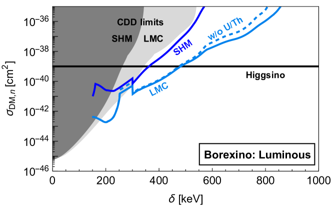
Figure 4: We show projections for the sensitivity of the Borexino experiment [17] to Higgsino dark matter using the luminous detection strategy, if Borexino were to analyze their existing data to search for this signal. Here, $\sigma_{\text{DM},n}$ is the DM-nucleon cross section, and $\delta$ is the mass splitting. These projections apply to any inelastic dark matter with a mass of $1.1~{}\text{TeV}$ and decay length much larger than the detector but much smaller than the Earth. The horizontal line indicates the actual cross section that Higgsinos would have in the minimal model. The projections assume our two different example halo models, the SHM and LMC. We have also illustrated the effect on the LMC curve when the uranium and thorium content of the Earth is neglected. The gray bands show the existing limits from collisional direct detection (CDD) experiments as in Figure 3, assuming the SHM (dark gray) or LMC (light gray) halo models.

In this section, we present the projections of the various luminous DM detection experiments and strategies described in this paper, using both the SHM and the LMC model. In addition to the Higgsino cross section of $\sigma_{\tilde{H}n}=10^{-39}~{}\text{cm}^{2}$, we also show results for a broader range of cross sections $\sigma_{\text{DM},n}$ that apply to more general models of inelastic DM with the same mass as the Higgsino, $m_{\tilde{H}}=1.1$ TeV, and the same decay length $l_{\tilde{H}_{2}}$ (eq. (4)), though the latter condition can be relaxed for the curves without Pb/U supplements. In all cases, we use Borexino’s total run time of $t_{\text{total}}=3628.7~{}\text{days}\approx 10~{}\text{years}$, although the signal is unsuppressed only half that time, $t_{\text{signal}}=t_{\text{total}}/2$, due to daily modulation. We assume the same total runtime for other upcoming experiments. All projections scale with the square root of time due to the presence of backgrounds, meaning that running the experiment for one year would yield constraints within a factor of $\approx 3$ of the limits shown here. The only exception is the background-free experiment (brown dash-dotted line in Figure 6), which improves linearly with time.

We first present in Figure 4 the projections for the Borexino experiment. This figure highlights the improvement enabled by the LMC model compared to the SHM; for Higgsino detection, this results in an improvement from $\delta^{\text{SHM}}_{\text{Borexino}}\sim 360$ keV to $\delta^{\text{LMC}}_{\text{Borexino}}\sim 480$ keV. We also show the result for the LMC model without including the terrestrial abundances of Th and U. The inclusion of these elements is evidently not relevant for the Higgsino line itself at Borexino (and they were not included in previous work [4]). However including Th and U immediately improves bounds at higher cross sections than $\sigma_{\tilde{H}n}=10^{-39}~{}\text{cm}^{2}$, and as we pull down the constraints curves (shown in later figures) with our improvement strategies, these elements will become important for the Higgsino as well. For example, these elements are important to include for SNO+ or JUNO in the LMC model. The limits in Figure 4 are attainable with Borexino’s existing $\sim 10$ year data, and we advocate for this analysis, as it represents the most cost-effective advancement currently available for Higgsino dark matter.

Several features in this plot are worth noting. Due to the large background rate coming from ${}^{14}\text{C}$ $\beta$-decay (see Figure 6 of Ref. [4]), there is a reduced sensitivity below $250$ keV, with a complete cutoff at the threshold of $E_{\text{thr}}=150$ keV. This reduced sensitivity is apparent in the SHM curve. However, in the LMC curve, this feature is overshadowed by a sharp downward turn at $\delta^{\text{LMC}}_{\text{max,Fe}}=250$ keV, resulting from the sudden availability of Fe for scattering below this threshold. The vast abundance of Fe—four orders of magnitude higher than Sr and Ba—enables much stronger sensitivity. In the SHM curve, due to the lower maximum velocity $v_{\text{max}}^{\text{SHM}}<v_{\text{max}}^{\text{LMC}}$, the Fe kink occurs at $\delta^{\text{SHM}}_{\text{max,Fe}}=~{}160$ keV. Meanwhile, the sharp decline below $\delta_{\text{{mantle,Ba}}}=300$ keV is due to the terrestrial abundance of Ba being a factor of $\sim 40$ lower in the mantle than in the crust (see Table 2), which we model as an abrupt transition at $30$ km depth (see Appendix A). These features are consistent across all subsequent figures.

In Figures 5 and 6, we present the projected limits of the SNO+ and JUNO experiments, respectively, with the SHM and the LMC model shown in different panels. The Higgsino sensitivities of the standard luminous detection scheme (shown in green) of SNO+ and JUNO are $\delta^{\text{LMC}}_{\text{SNO}}\sim 500$ keV and $\delta^{\text{LMC}}_{\text{JUNO}}\sim 580$ keV, respectively; they are also shown in Figure 1 in green and red blocks. These curves improve over Borexino by the square root of their detector volumes, as we assume the background per scintillator mass is equal across experiments.

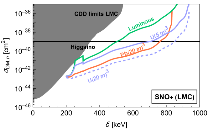
(a) Sensitivities assuming our example LMC halo model.

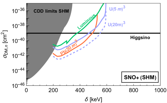
(b) Sensitivities assuming our example SHM.

Figure 5: Projected sensitivity for the SNO+ experiment [51] in the DM-nucleon cross section $\sigma_{\text{DM},n}$ vs splitting $\delta$, if the luminous detection analysis discussed here is carried out. We also show projections if extra heavy material is placed near SNO+ using as example scenarios: $(5\,\text{m})^{3}$ of uranium and $(20\,\text{m})^{3}$ of lead or uranium. The two different figures show sensitivities assuming our two different example halo models (a) LMC and (b) SHM. The luminous projection in green applies to any inelastic dark matter with a mass of $1.1~{}\text{TeV}$ and decay length much larger than the detector but much smaller than the Earth. The projections with supplemental Pb/U also assume that the decay length is the same as that of the Higgsino. The horizontal line shows the actual cross section that Higgsinos would have in the minimal model. Shown in gray are current limits from collisional direct detection (CDD) experiments as in Figure 3.

We also show the enhanced sensitivity SNO+ and JUNO would achieve if a large volume of supplemental Pb (orange lines) or U (purplish-blue lines) is installed near the detector, as described in Section VI.1. Since this method may be limited by the available space near the detector (and potentially by the cost of excavating additional volume), we report the results based on the volume of the supplemental Pb/U, considering the benchmark volumes of $(5~{}\text{m})^{3}$ and $(20~{}\text{m})^{3}$. Pb has a cutoff point of $\delta^{\text{LMC}}_{\text{max,Pb}}=830$ keV, beyond which the supplemental Pb no longer contributes. With $(20~{}\text{m})^{3}$ of supplemental Pb, SNO+ and JUNO approach Higgsino sensitivities near this limit. Encouragingly, the sensitivity of just $(5~{}\text{m})^{3}$ of U performs only slightly worse, despite the volume being 64 times smaller. With $(20~{}\text{m})^{3}$ of U, JUNO’s Higgsino bound can reach $\delta^{\text{LMC}}_{\text{JUNO,U}}\sim 870$ keV, while SNO+ follows closely at $\delta^{\text{LMC}}_{\text{SNO,U}}\sim 850$ keV. These limits are shown in Figure 1 in purple and brown, labeled “+Pb” and “+U.”

We also include in Figure 6 projections of a background-free gamma-ray detector (shown by the brown dash-dotted line) with the same $17.5$-meter radius as JUNO, as discussed in Section VI.2. Such a detector can probe splittings upto $\delta^{\text{LMC}}_{\text{BGF}}\sim 830$ keV for the Higgsino. We emphasize that this is a preliminary idea, and further research is needed to determine the feasibility of such a background-free detector. While complete elimination of background may not be achievable in practice, we present this background-free curve as an ultimate limit. Additionally, supplemental U could be installed around the background-free detector. In this most optimistic scenario, $(20~{}\text{m})^{3}$ of U (not shown) is sufficient to fully saturate the $\delta^{\text{LMC}}_{\text{max,U}}\sim 940$ keV limit.

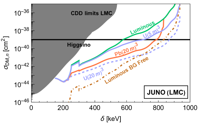
(a) Sensitivities assuming our example LMC halo model.

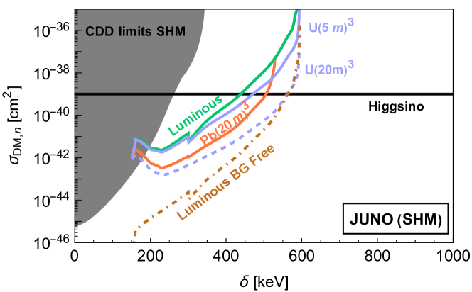
(b) Sensitivities assuming our example SHM.

Figure 6: Same as Figure 5 except for the JUNO experiment [18] instead of SNO+. Here, we also plot a curve for a background-free detector the same size as JUNO, to demonstrate the limit of background reduction.

VIII Conclusion

In this work, we studied the feasibility of terrestrial detection for one of the few theoretically well-motivated WIMPs that have still survived: the pseudo-Dirac Higgsino. Its splitting has been constrained to $\delta\gtrsim 260$ keV from traditional direct detection in existing literature, assuming the SHM for dark matter velocity. In this work, we showed that incorporating the additional fast component of dark matter, due to the merger of the LMC with the MW, improves these constraints to larger splitting, $\delta\gtrsim 340~{}\textrm{keV}$. We also noted that a “luminous” detection strategy, where Higgsinos scatter off the Earth and subsequently decay in large-volume neutrino detectors producing a mono-energetic photon, shows great promise for pushing to much higher $\delta$. Such a detection strategy also benefits from the faster dark matter in the LMC halo model, as well as the presence of heavy elements such as U and Th in the Earth. A reanalysis of the 10-year Borexino dataset searching for this luminous signal could probe Higgsinos with splittings up to $\sim 500$ keV. Larger detectors, such as SNO+ and JUNO, show exciting promise due to their larger fiducial volumes. Additionally, placing large amounts of Pb or U next to these detectors could further improve sensitivity, reaching splittings of up to $\sim 900$ keV.

It is important to note that probing splittings in the hundreds of keV range corresponds to gauginos with masses above the PeV scale. This mass range is beyond the reach of even future colliders or precision EDM experiments, and thus, it is not expected to be probed by other means in the near future. The methods introduced in this paper provide a complementary probe of smaller mass splittings, with splittings much larger than 10 MeV being expected to be probed by Advanced ACME and direct detection via Higgs scattering (see Figure 1). Even future projections are going to leave a tantalizing unconstrained window between $1$ MeV and $30$ MeV. Finding novel ideas to probe this window for one of the last surviving WIMP candidates is an open problem.

We emphasize that the $1.1$ TeV Higgsino is not the sole beneficiary of the ideas introduced in this work, namely, incorporation of the high-speed LMC dark matter population, consideration of heavy elements like Th and U in the Earth’s crust, and supplementation with large blocks of heavy metal. Any inelastic dark matter candidate with mass splitting and subsequent decay of the excited state into Standard Model particles can be searched for with this technique, as long as the decay length is macroscopic and smaller than the size of the Earth. Models such as Higgsino dark matter with masses different from $1.1$ TeV, which might arise from non-standard cosmologies or other electroweak n-plets with non-zero hypercharge, are excellent examples. Another candidate is the magnetic inelastic dark matter scenario. We will discuss limits and projections for these models in forthcoming work.

Appendix A Terrestrial Element Abundances

Our sensitivity is set by the number densities $n_{A}$ of the elements in the Earth, but they are often reported in mass abundances $a_{A}$ (i.e., mass fraction). The two quantities are related by

$$n_{A}=a_{A}\times\frac{N_{0}}{M_{A}}\rho~{},$$ (35)

where $N_{0}$ is Avogadro’s number, $M_{A}$ is the molar mass, and $\rho$ is the density of the Earth. However, the Earth’s density and the elemental abundances vary with depth. For this calculation, we need only consider the crust and mantle, which have average densities $\rho_{\text{crust}}=2830~{}\text{kg}/\text{m}^{3}$ [52] and $\rho_{\text{mantle}}=4500~{}\text{kg}/\text{m}^{3}$ [53]. We will also take into account the elemental abundances in conjunction with the characteristic decay lengths $l_{\text{max},A}$ (eq. (25)).

The first $\sim 30$ km below Earth’s surface constitutes the Earth’s crust, which can be divided into the upper, middle, and lower crust, each with different elemental abundances. Instead of treating all three layers separately, we note that for the four heaviest elements listed in Table 2, each has significantly lower abundances than the next heaviest element on our list, making their contributions important only above the $\delta_{\text{max},A}$ of the preceding element. This simplifies our calculation, as we can safely assume most of these elements have constant abundances. In effect, since the upper crust is estimated to be $\sim 15$ km thick [40], and Ba has a characteristic decay length ($l^{\text{LMC}}_{\text{max,Ba}}=5.8$ km) well within the upper crust, we can use the upper-crust abundances of Pb, Th, and U, even though these elements are less abundant in the middle and lower crust [40].

Sr and Ba have appreciable abundances in both the mantle and the crust, but their number densities in the mantle are about an order of magnitude lower than their values in the crust. To account for this, we compute the $\delta$ at which the corresponding decay length reaches $30$ km depth, using the minimum velocity required to scatter the given element (eq. (11)). This calculation yields

$$\delta_{\text{mantle,A}}=300~{}\text{keV}\left(\frac{117~{}\text{GeV}}{\mu_{A}}\right)^{1/5}~{}.$$ (36)

For instance, for $\delta<\delta_{\text{mantle,Ba}}=300$ keV, we use Ba’s mantle number density; otherwise, we use its crust density. We do not need to repeat this calculation for Ca and Fe, since $\delta_{\text{mantle,Ca}}=380~{}\text{keV}$ and $\delta_{\text{mantle,Fe}}=360~{}\text{keV}$ are well above $\delta^{\text{LMC}}_{\text{max},\text{Ca}}=180~{}\text{keV}$ and $\delta^{\text{LMC}}_{\text{max},\text{Fe}}=250~{}\text{keV}$; see Table 2. Thus, only their mantle abundances are relevant.

References

- Hall et al. [1998] L. J. Hall, T. Moroi, and H. Murayama, Sneutrino cold dark matter with lepton number violation, Phys. Lett. B 424, 305 (1998), arXiv:hep-ph/9712515 .
- Tucker-Smith and Weiner [2001] D. Tucker-Smith and N. Weiner, Inelastic dark matter, Phys. Rev. D 64, 043502 (2001), arXiv:hep-ph/0101138 .
- Feldstein et al. [2010] B. Feldstein, P. W. Graham, and S. Rajendran, Luminous Dark Matter, Phys. Rev. D 82, 075019 (2010), arXiv:1008.1988 [hep-ph] .
- Eby et al. [2019] J. Eby, P. J. Fox, R. Harnik, and G. D. Kribs, Luminous Signals of Inelastic Dark Matter in Large Detectors, JHEP 09, 115, arXiv:1904.09994 [hep-ph] .
- Pospelov et al. [2014] M. Pospelov, N. Weiner, and I. Yavin, Dark matter detection in two easy steps, Phys. Rev. D 89, 055008 (2014), arXiv:1312.1363 [hep-ph] .
- Meng et al. [2021] Y. Meng, Z. Wang, Y. Tao, A. Abdukerim, Z. Bo, W. Chen, X. Chen, Y. Chen, C. Cheng, Y. Cheng, X. Cui, Y. Fan, D. Fang, C. Fu, M. Fu, L. Geng, K. Giboni, L. Gu, X. Guo, K. Han, C. He, J. He, D. Huang, Y. Huang, Z. Huang, R. Hou, X. Ji, Y. Ju, C. Li, M. Li, S. Li, S. Li, Q. Lin, J. Liu, X. Lu, L. Luo, W. Ma, Y. Ma, Y. Mao, N. Shaheed, X. Ning, N. Qi, Z. Qian, X. Ren, C. Shang, G. Shen, L. Si, W. Sun, A. Tan, A. Wang, M. Wang, Q. Wang, S. Wang, S. Wang, W. Wang, X. Wang, M. Wu, W. Wu, J. Xia, M. Xiao, X. Xiao, P. Xie, B. Yan, X. Yan, J. Yang, Y. Yang, C. Yu, J. Yuan, Y. Yuan, D. Zhang, M. Zhang, P. Zhang, T. Zhang, L. Zhao, Q. Zheng, J. Zhou, N. Zhou, X. Zhou, and Y. Zhou (PandaX-4T Collaboration), Dark matter search results from the pandax-4t commissioning run, Phys. Rev. Lett. 127, 261802 (2021).
- Adams et al. [2023] E. Adams et al. (PICO), Search for inelastic dark matter-nucleus scattering with the PICO-60 CF3I and C3F8 bubble chambers, Phys. Rev. D 108, 062003 (2023), arXiv:2301.08993 [astro-ph.CO] .
- acme@ physics. harvard. edu 2 d Doyle JM 1 Gabrielse G. 1 3 Haefner J. 1 Hutzler NR 1 4 Lasner Z. 2 Meisenhelder C. 1 O’Leary BR 2 Panda CD 1 West AD 2 6 6 West EP 1 6 6 Wu X. 1 2 [2018] A. C. A. V. . . . A. D. . D. D. acme@ physics. harvard. edu 2 d Doyle JM 1 Gabrielse G. 1 3 Haefner J. 1 Hutzler NR 1 4 Lasner Z. 2 Meisenhelder C. 1 O’Leary BR 2 Panda CD 1 West AD 2 6 6 West EP 1 6 6 Wu X. 1 2, Improved limit on the electric dipole moment of the electron, Nature 562, 355 (2018).
- Krall and Reece [2018] R. Krall and M. Reece, Last Electroweak WIMP Standing: Pseudo-Dirac Higgsino Status and Compact Stars as Future Probes, Chin. Phys. C 42, 043105 (2018), arXiv:1705.04843 [hep-ph] .
- Aaboud et al. [2018] M. Aaboud, G. Aad, B. Abbott, O. Abdinov, B. Abeloos, S. H. Abidi, O. AbouZeid, N. L. Abraham, H. Abramowicz, H. Abreu, et al., Search for electroweak production of supersymmetric states in scenarios with compressed mass spectra at s= 13 tev with the atlas detector, Physical Review D 97, 052010 (2018).
- Rinchiuso et al. [2021] L. Rinchiuso, O. Macias, E. Moulin, N. L. Rodd, and T. R. Slatyer, Prospects for detecting heavy WIMP dark matter with the Cherenkov Telescope Array: The Wino and Higgsino, Phys. Rev. D 103, 023011 (2021), arXiv:2008.00692 [astro-ph.HE] .
- Rodd et al. [2024] N. L. Rodd, B. R. Safdi, and W. L. Xu, CTA and SWGO can discover Higgsino dark matter annihilation, Phys. Rev. D 110, 043003 (2024), arXiv:2405.13104 [hep-ph] .
- Actis et al. [2011] M. Actis et al. (CTA Consortium), Design concepts for the Cherenkov Telescope Array CTA: An advanced facility for ground-based high-energy gamma-ray astronomy, Exper. Astron. 32, 193 (2011), arXiv:1008.3703 [astro-ph.IM] .
- Co et al. [2022] R. T. Co, B. Sheff, and J. D. Wells, Race to find split Higgsino dark matter, Phys. Rev. D 105, 035012 (2022), arXiv:2105.12142 [hep-ph] .
- Haber and Wyler [1989] H. E. Haber and D. Wyler, Radiative neutralino decay, Nuclear Physics B 323, 267 (1989).
- Bramante et al. [2016] J. Bramante, P. J. Fox, G. D. Kribs, and A. Martin, Inelastic frontier: Discovering dark matter at high recoil energy, Phys. Rev. D 94, 115026 (2016), arXiv:1608.02662 [hep-ph] .
- Basilico et al. [2023] D. Basilico et al. (BOREXINO), Final results of Borexino on CNO solar neutrinos, Phys. Rev. D 108, 102005 (2023), arXiv:2307.14636 [hep-ex] .
- Djurcic et al. [2015] Z. Djurcic et al. (JUNO), JUNO Conceptual Design Report, (2015), arXiv:1508.07166 [physics.ins-det] .
- Albanese et al. [2021] V. Albanese et al. (SNO+), The SNO+ experiment, JINST 16 (08), P08059, arXiv:2104.11687 [physics.ins-det] .
- Song et al. [2021] N. Song, S. Nagorny, and A. C. Vincent, Pushing the frontier of WIMPy inelastic dark matter: Journey to the end of the periodic table, Phys. Rev. D 104, 103032 (2021), arXiv:2104.09517 [hep-ph] .
- Digman et al. [2019] M. C. Digman, C. V. Cappiello, J. F. Beacom, C. M. Hirata, and A. H. G. Peter, Not as big as a barn: Upper bounds on dark matter-nucleus cross sections, Phys. Rev. D 100, 063013 (2019), [Erratum: Phys.Rev.D 106, 089902 (2022)], arXiv:1907.10618 [hep-ph] .
- Smith-Orlik et al. [2023] A. Smith-Orlik et al., The impact of the Large Magellanic Cloud on dark matter direct detection signals, JCAP 10, 070, arXiv:2302.04281 [astro-ph.GA] .
- Grothaus et al. [2014] P. Grothaus, M. Fairbairn, and J. Monroe, Directional Dark Matter Detection Beyond the Neutrino Bound, Phys. Rev. D 90, 055018 (2014), arXiv:1406.5047 [hep-ph] .
- Drukier et al. [1986] A. K. Drukier, K. Freese, and D. N. Spergel, Detecting cold dark-matter candidates, Phys. Rev. D 33, 3495 (1986).
- Lisanti [2017] M. Lisanti, Lectures on Dark Matter Physics, in Theoretical Advanced Study Institute in Elementary Particle Physics: New Frontiers in Fields and Strings (2017) pp. 399–446, arXiv:1603.03797 [hep-ph] .
- Evans et al. [2019] N. W. Evans, C. A. J. O’Hare, and C. McCabe, Refinement of the standard halo model for dark matter searches in light of the Gaia Sausage, Phys. Rev. D 99, 023012 (2019), arXiv:1810.11468 [astro-ph.GA] .
- Evans and An [2006] N. W. Evans and J. H. An, Distribution function of the dark matter, Phys. Rev. D 73, 023524 (2006), arXiv:astro-ph/0511687 .
- Vogelsberger et al. [2009] M. Vogelsberger, A. Helmi, V. Springel, S. D. M. White, J. Wang, C. S. Frenk, A. Jenkins, A. D. Ludlow, and J. F. Navarro, Phase-space structure in the local dark matter distribution and its signature in direct detection experiments, Mon. Not. Roy. Astron. Soc. 395, 797 (2009), arXiv:0812.0362 [astro-ph] .
- Zemp et al. [2009] M. Zemp, J. Diemand, M. Kuhlen, P. Madau, B. Moore, D. Potter, J. Stadel, and L. Widrow, The Graininess of Dark Matter Haloes, Mon. Not. Roy. Astron. Soc. 394, 641 (2009), arXiv:0812.2033 [astro-ph] .
- Kuhlen et al. [2010] M. Kuhlen, N. Weiner, J. Diemand, P. Madau, B. Moore, D. Potter, J. Stadel, and M. Zemp, Dark Matter Direct Detection with Non-Maxwellian Velocity Structure, JCAP 02, 030, arXiv:0912.2358 [astro-ph.GA] .
- Mao et al. [2014] Y.-Y. Mao, L. E. Strigari, and R. H. Wechsler, Connecting Direct Dark Matter Detection Experiments to Cosmologically Motivated Halo Models, Phys. Rev. D 89, 063513 (2014), arXiv:1304.6401 [astro-ph.CO] .
- Besla et al. [2019] G. Besla, A. Peter, and N. Garavito-Camargo, The highest-speed local dark matter particles come from the Large Magellanic Cloud, JCAP 11, 013, arXiv:1909.04140 [astro-ph.GA] .
- Donaldson et al. [2022] K. Donaldson, M. S. Petersen, and J. Peñarrubia, Effects on the local dark matter distribution due to the large magellanic cloud, Monthly Notices of the Royal Astronomical Society: Letters 513, 46–51 (2022).
- Besla et al. [2007] G. Besla, N. Kallivayalil, L. Hernquist, B. Robertson, T. J. Cox, R. P. van der Marel, and C. Alcock, Are the Magellanic Clouds on their First Passage about the Milky Way?, Astrophys. J. 668, 949 (2007), arXiv:astro-ph/0703196 .
- Grand et al. [2017] R. J. J. Grand, F. A. Gómez, F. Marinacci, R. Pakmor, V. Springel, D. J. R. Campbell, C. S. Frenk, A. Jenkins, and S. D. M. White, The Auriga Project: the properties and formation mechanisms of disc galaxies across cosmic time, Mon. Not. Roy. Astron. Soc. 467, 179 (2017), arXiv:1610.01159 [astro-ph.GA] .
- Klypin et al. [2002] A. Klypin, H. Zhao, and R. S. Somerville, Lambda CDM-based models for the Milky Way and M31 I: Dynamical models, Astrophys. J. 573, 597 (2002), arXiv:astro-ph/0110390 .
- Read [2014] J. I. Read, The Local Dark Matter Density, J. Phys. G 41, 063101 (2014), arXiv:1404.1938 [astro-ph.GA] .
- Salem et al. [2015] M. Salem, G. Besla, G. Bryan, M. Putman, R. P. van der Marel, and S. Tonnesen, Ram pressure stripping of the large magellanic cloud’s disk as a probe of the milky way’s circumgalactic medium, The Astrophysical Journal 815, 77 (2015).
- Yuan et al. [2022] Y. Yuan et al. (PandaX), A search for two-component Majorana dark matter in a simplified model using the full exposure data of PandaX-II experiment, Phys. Lett. B 832, 137254 (2022), arXiv:2205.08066 [hep-ex] .
- Rudnick and Gao [2014] R. Rudnick and S. Gao, 4.1 - composition of the continental crust, in Treatise on Geochemistry (Second Edition), edited by H. D. Holland and K. K. Turekian (Elsevier, Oxford, 2014) second edition ed., pp. 1–51.
- Palme and O’Neill [2014] H. Palme and H. O’Neill, 3.1 - cosmochemical estimates of mantle composition, in Treatise on Geochemistry (Second Edition), edited by H. D. Holland and K. K. Turekian (Elsevier, Oxford, 2014) second edition ed., pp. 1–39.
- World Nuclear Association [2023] World Nuclear Association, Uranium and depleted uranium (2023), accessed: 2024-09-10.
- Mazzitelli et al. [2019] G. Mazzitelli et al. (CYGNUS), CYGNO: a CYGNUs Collaboration 1 m3 Module with Optical Readout for Directional Dark Matter Search, (2019), arXiv:1901.04190 [physics.ins-det] .
- De Angelis et al. [2021] A. De Angelis, V. Tatischeff, A. Argan, S. Brandt, A. Bulgarelli, A. Bykov, E. Costantini, R. C. d. Silva, I. A. Grenier, L. Hanlon, D. Hartmann, M. Hernanz, G. Kanbach, I. Kuvvetli, P. Laurent, M. N. Mazziotta, J. McEnery, A. Morselli, K. Nakazawa, U. Oberlack, M. Pearce, J. Rico, M. Tavani, P. v. Ballmoos, R. Walter, X. Wu, S. Zane, A. Zdziarski, and A. Zoglauer, Gamma-ray astrophysics in the mev range: The astrogam concept and beyond, Experimental Astronomy 51, 1225–1254 (2021).
- Agostini et al. [2015] M. Agostini et al. (Borexino), A test of electric charge conservation with Borexino, Phys. Rev. Lett. 115, 231802 (2015), arXiv:1509.01223 [hep-ex] .
- Leo [1987] W. R. Leo, Techniques for Nuclear and Particle Physics Experiments: A How to Approach (1987).
- Machado et al. [2012] P. A. N. Machado, T. Muhlbeier, H. Nunokawa, and R. Zukanovich Funchal, Potential of a Neutrino Detector in the ANDES Underground Laboratory for Geophysics and Astrophysics of Neutrinos, Phys. Rev. D 86, 125001 (2012), arXiv:1207.5454 [hep-ph] .
- Bertou [2013] X. Bertou, The andes deep underground laboratory (2013), arXiv:1308.0059 [astro-ph.IM] .
- JUNO Collaboration [2022] JUNO Collaboration, Juno physics and detector, Progress in Particle and Nuclear Physics 123, 103927 (2022).
- Simms [2024] J. Simms, Muon Track Reconstruction in the Scintillator Phase of SNO+, in Prospects in Neutrinos Physics (2024) arXiv:2404.03680 [physics.ins-det] .
- Andringa et al. [2016] S. Andringa et al. (SNO+), Current Status and Future Prospects of the SNO+ Experiment, Adv. High Energy Phys. 2016, 6194250 (2016), arXiv:1508.05759 [physics.ins-det] .
- Christensen and Mooney [1995] N. I. Christensen and W. D. Mooney, Seismic velocity structure and composition of the continental crust: A global view, Journal of Geophysical Research: Solid Earth 100, 9761 (1995), https://agupubs.onlinelibrary.wiley.com/doi/pdf/10.1029/95JB00259 .
- Webb [2023] P. Webb, Introduction to Oceanography (Pressbooks, 2023).