Optimal control for coupled sweeping processes under minimal assumptions

Abstract

In this paper, the study of nonsmooth optimal control problems $(P)$ involving a controlled sweeping process with three main characteristics is launched. First, the sweeping sets $C(t)$ are nonsmooth, unbounded, time-dependent, uniformly prox-regular, and satisfy minimal assumptions. Second, the sweeping process is coupled with a controlled differential equation. Third, joint-state endpoints constraint set $S$, including periodic conditions, is present. This general model incorporates different important controlled submodels as particular cases, such as subclasses of second order sweeping processes and of integro-differential sweeping processes, coupled evolution variational inequalities (EVI), and Bolza-type problems. The existence and uniqueness of a Lipschitz solution for the Cauchy problem associated with our dynamic is established, the existence of an optimal solution for our general form of optimal control is obtained, and the full form of the nonsmooth Pontryagin maximum principle for strong local minimizers in $(P)$ is derived under minimal hypotheses. One of the novelties of this paper in accomplishing the latter goal for unbounded sweeping sets with local constraint qualifications, is the idea to work with a well-constructed problem corresponding to truncated sweeping sets and joint endpoint constraints, that shares the same strong local minimizer as $(P)$ and for which the exponential-penalty approximation technique can be developed using only the assumptions on $(P)$. The presence of the truncation renders this development quite involved and tedious. The utility of the optimality conditions is illustrated with an example.

1. Introduction and Preliminaries

1.1. Introduction

Sweeping process. J.J. Moreau introduced the sweeping process as being a differential inclusion in which the set-valued map is the normal cone to a nicely moving closed set $C(t)$, called the sweeping set (see [36, 37, 38]). Its simplest form is given by

$$\dot{x}(t)\in-N_{C(t)}(x(t)),\;\text{ a.e. }t\in[0,T].$$

When $C(t)\subset\mathbb{R}^{n}$ is a non-empty convex closed set, $N_{C(t)}$ is taken to be the normal cone of convex analysis. When $C(t)$ is non-convex, as is the case of this paper, $N_{C(t)}$ denotes the Clarke normal cone and the set $C(t)$ is commonly taken to be uniformly prox-regular. When a perturbation or external force $f$ exists, we call the dynamic a perturbed sweeping process, and when $f$ depends on a control $u$, we call it a perturbed controlled sweeping process.
Sweeping processes appear in many applications including elastoplasticity, hysteresis, ferromagnetism, electric circuits, phase transitions, traffic equilibrium, etc., see, for instance, [1, 4, 7, 34, 48]. During the last decade, the study of sweeping process has intensified due to their natural presence in newly developed applications such as the mobile robot model [21], the pedestrian traffic flows model [21], and the crowd motion model for emergency evacuation (see, e.g., [8] and [11]). In these models, the main concern is to control the state of events efficiently, that is, to optimize a certain objective function over controlled sweeping process.
Optimal control over sweeping process. Due to the unboundedness and discontinuity of the normal cone, standard results on differential inclusions cannot be used for sweeping processes. Extensive literature exists on the question of existence and uniqueness of an absolutely continuous or Lipschitz solution for the Cauchy problem associated with different forms of the following perturbed controlled sweeping process

$$\dot{x}(t)\in f(t,x(t),u(t))-N_{C(t)}(x(t))\text{ a.e. }t\in[0,T],\;x(0)=x_{0}\in C(0),$$ (1)

in which the constraint $x(t)\in C(t)$ is implicit. However, such results commonly require the sets $C(t)$ to move in an absolutely continuous or Lipschitz manner (see e.g., [28]). On the other hand, numerous efforts have been made to derive existence theory for optimal solutions and/or necessary conditions in terms of Euler-Lagrange equation or Pontryagin-type maximum principle for optimal control problems driven by variants of (1). The main approach used to solve different versions of such a problem is the method of approximation, either discrete (see e.g., [9, 10, 11, 12, 18, 19, 20, 22]), or continuous (exponential penalty-type) (see [6, 23, 26, 27, 41, 42, 43, 50]). Our focus in this paper is on the latter.
Continuous approximation method. The exponential penalization technique was first used in [23, 24] to derive Pontryagin-type maximum principle for global minimizers of a Mayer problem over (1), in which $f$ is smooth, $C$ is a constant compact set defined as the zero-sublevel set of a $\mathcal{C}^{2}$-convex function $\psi$ satisfying a constraint qualification on $\mathbb{R}^{n}$, the initial state-constraint is a set $C_{0}\subset C$, and the final state is free. The importance of this technique resides in approximating $N_{C}(\cdot)$ by the exponential penalty term $\gamma_{k}e^{\gamma_{k}\psi(\cdot)}\nabla\psi(\cdot)$ such that the so-obtained approximating dynamic is a standard control system without state constraints, but for which the set $C$ is invariant:

$$\dot{x}(t)=f(t,x(t),u(t))-\gamma_{k}e^{\gamma_{k}\psi(x(t))}\nabla\psi(x(t))\text{ a.e.},\;\;x(0)=x_{0}\in C(0).$$ (2)

The absence in (2) of the explicit state constraint, $x(t)\in C$, that is implicitly present in (1), has also shown to be instrumental in constructing numerical algorithms for controlled sweeping processes (see [25, 40, 44]). The domain of applicability of the exponential penalization technique for the results in [23, 24] was later enlarged in [50, 41, 43], to include strong local minimizers for controlled sweeping processes having: nonsmooth perturbation $f,$ a final state constraint set $C_{T}\subset\mathbb{R}^{n}$, the cost depends on both state-endpoints, a constant sweeping set $C$ that is nonsmooth (i.e., $C$ is the intersection of a finite number of zero-sublevel sets of $\mathcal{C}^{1,1}$-generators $\psi_{1}(x),\cdots,\psi_{r}(x)$ near $C$), the functions $\psi_{i}$’s satisfy a constraint qualification on $C$, and $C$ belongs to a certain class of unbounded sets that includes convex, compact, or polyhedral sets. In addition, the normal cone, $N_{C}$, in (1) is replaced therein, by a subdifferential, $\partial\varphi$, of a function $\varphi$ with domain $C$, which is shown to be equivalent to the study of (1) with a different $f$. In [26] and later in [27] (independently from [43]), the authors extended, under the compactness of Gr $C(\cdot)$, their previous smooth Pontryagin principle for global minimizers in [23] to the case where the sweeping set $C(t)$ is time-dependent and nonsmooth with $\mathcal{C}^{2}$- generators $(\psi_{i}(t,x))_{i=1}^{r}$ satisfying a global constraint qualification, and the final state is a compact set $C_{T}\subset C(T).$ In [31], a different approach is used to establish a form of nonsmooth Pontryagin maximum principle for strong local minimizers of the problem in [27], in which the initial state is fixed, the final state is free, and $C(\cdot)$Lipschitz.

Our model and its applications. Our optimal control problem ($P$), introduced in Section 2 and governed by the following dynamic $(D)$, where $x(t)\in\mathbb{R}^{n}$ and $y(t)\in\mathbb{R}^{l}$,

$$(D)\begin{cases}\dot{x}(t)\in f(t,x(t),y(t),u(t))-N_{C(t)}(x(t)),\text{ a.e. }t\in[0,T],\\ \dot{y}(t)=g(t,x(t),y(t),u(t)),\text{ a.e. }t\in[0,T],\\ \end{cases}$$

is distinguished by having three new features, namely, $(i)$ a controlled sweeping process coupled with a standard controlled differential equation, $(ii)$ a time-dependent, unbounded, and nonsmooth sweeping set that satisfies minimal assumptions, and $(iii)$ joint state endpoints constraint set $S$. Our model incorporates different controlled submodels as particular cases: coupled evolution variational inequalities (see [1], [3], [6]), a subclass of Integro-Differential sweeping processes of Volterra type (see [5]), second order sweeping processes, in which the sweeping set is solely time-dependent (see, e.g., [39] for the general setting), and Bolza-type problems associated to $(P)$. In other words, optimal control problems governed by either of the four submodels can readily be formulated as a special case of ($P$), and hence, all the results of this paper are applicable to these models.
Our findings and results. This paper presents a generalization and extension in different directions of all the previous results aforementioned in this introduction. Indeed, this paper establishes local and global results for the hybrid problem $(P)$. The first result, which is local, is given in Theorem 2.1 and consists of deriving under minimal assumptions on the data, a complete set of necessary conditions in the form of nonsmooth Pontryagin maximum principle for strong local minimizers of the problem ($P$) via developing the exponential penalization technique. The second and third results, which are global, encompass the existence and uniqueness of a Lipschitz solution for the Cauchy problem corresponding to our dynamic $(D)$ without requiring any Lipschitz property on $C(\cdot)$ (Theorem 2.2), as well as the global existence of optimal solution for our problem (Theorem 2.3). This latter and the Pontryagin principle (Theorem 2.1) constitute the first attempt to obtain these results for such general problems.
One might wonder whether in our proofs here, the differential equation in $(D)$ could be included in a sweeping process, where $X(t)\mathrel{\mathop{\mathchar 58\relax}}=(x(t),y(t))$ and the sweeping set would be $A(t)\mathrel{\mathop{\mathchar 58\relax}}=C(t)\times\mathbb{R}^{l}$. Although this approach might be sufficient for proving the local result, i.e., the maximum principle, by means of the localization technique developed in Section 3, however, it fails to work for our global results (Theorems 2.2 and 2.3) due to the unbounded nature of $A(t)$.

Note that even for the special case when $(D)$ consists of only the sweeping process, this paper constitutes the first attempt to prove existence result of optimal solutions, Theorem 2.3, for time-dependent sweeping set or for joint-endpoint constraints; as in the literature the only papers studying optimality for our form of $C(t)$, i.e., [27] and [31], do not cover this question, and the joint-state endpoints were never considered before with sweeping processes. Furthermore, our Pontryagin maximum principle, Theorem 2.1, generalizes all previously known results in multiple ways. Unlike the corresponding results known for special cases of our problem in [23, 24, 26, 27, 50, 41, 43], all the assumptions, including the constraint qualification, are assumed locally around the optimal state, and unlike the special case treated in [31], the set valued map is not assumed to be Lipschitz. In addition to localizing the constraint qualification (see (A3.2)), the results in [43] are extended to the case when their form of $C$ is now any unbounded and time-dependent set, the state endpoints are joint, and the convexity assumption of the sets $f(t,x,U(t))$ is now discarded not only for the free final endpoint case, but rather for general joint-endpoint constraints. Note that, in our maximum principle and similarly to [41, 43], where $C$ is constant, the nontriviality condition is simply $\lambda+\|p(T)\|=1$ and does not invoke the measure corresponding to $x(t)\in{C(t)}$, and new subdifferentials that are strictly smaller than the Clarke and Mordukhovich subdifferentials are used. In addition to this latter advantage regarding the subdifferentials, the results in [27] are generalized to (a) strong local minimizers, (b) joint state endpoints, (c) $f$ nonsmooth and $\psi_{i}$ $\in$ $\mathcal{C}^{1,1}$ ($\forall i$), (d) $f(t,x,U)$ not convex, (e) $U$ time-dependent, (f) graph of $C(\cdot)$ is unbounded, (g) $C(t)$ having no restriction on its corners and no extra assumptions on the gradients of its generators, and (h) localized hypotheses on the data and on all the imposed assumptions including local constraint qualification and local diagonal dominance of the Gramian matrix (see (A3.2)-(A3.3)). While the approach in [31] does not require the diagonal dominance of the Gramian matrix, it demands that their sweeping set $C(\cdot)$ must adhere to a Lipschitz condition, with a fixed initial state and free final state $-$ restrictions which are not imposed for our result. Moreover, in the maximum principle therein, instead of the standard nontriviality condition ($\lambda=1$ in their case), an atypical nondegeneracy condition is obtained, and the standard Clarke and Mordukhovich subdifferentials are utilized.
Novelty of the methods employed. Although our nonsmooth sweeping set here is time-dependent as in [27], the exponential penalization approach employed therein to derive Pontryagin-type principle is not useful here for three main reasons. One is that, in [27], the sets $C(t)$ are approximated from the outside by larger sets $C^{k}(t)$, and hence, the states $x_{k}(t)\in C^{k}(t)$ approximating the optimal state $\bar{x}$ do not necessarily lie in the interior of $C(t)$. This would lead to having the maximum principle formulated in terms of the standard subdifferentials, which are larger than the subdifferentials used in our maximum principle. Second, even if we modify the approximating sets $C^{k}(t)$ of $C(t)$ to be in $\textnormal{int}\,C(t)$, then, the invariance property of $C^{k}(t)$ or $C(t)$ itself which is the back bone of this approach, would not be established without imposing a highly restrictive assumption on the corners of $C(t)$ as in [27]. This assumption excludes simple geometric shapes for $C(t)$, e.g., triangles, etc. Third, even if we approximate the sweeping set $C(t)$ from its interior, their approach requires imposing the boundedness on the graph of $C(\cdot)$ and a global constraint qualification in a band around $C(t)$.
The first two reasons can be addressed by extending to our general setting the penalization approach in [41, 43], that will allow us to approximate $C(t)$ by sets $C^{\gamma_{k}}(t,k)$ in the interior of $C(t)$. This idea is fruitful when establishing the existence of solution for the Cauchy Problem associated with $(D)$ (see the proof of Theorem 2.2). However, this approach is not adequate for our Pontryagin principle, because it does not address the third reason, as it also requires global constraint qualifications on $C(t)$, like [27], and does not apply to general unbounded sweeping sets.
In this paper, we establish the Pontryagin principle for a $\bar{\delta}$-strong local minimizer $((\bar{x},\bar{y}),\bar{u})$ of $(P)$ without assuming the boundedness of the graph of $C(\cdot)$ and under merely a local constraint qualification on the generators of $C(t)$, $(\psi_{i}(t,x))_{i=1}^{r}$, at the graph of $\bar{x}$ (see (A3.2)). To reach this goal, we introduce in (16) a new dynamic of sweeping processes, $(\bar{D})$, obtained from $(D)$ through truncating the given prox-regular sweeping sets $C(t)$ and the space $\mathbb{R}^{l}$ by respectively the balls $\bar{B}_{\bar{\varepsilon}}(\bar{x}(t))$ and $\bar{B}_{\bar{\delta}}(\bar{y}(t))$, where $\bar{\varepsilon}\in(0,\bar{\delta})$ is a specific radius particularily chosen so that the bounded truncated sets $C(t)\cap\bar{B}_{\bar{\varepsilon}}(\bar{x}(t))$ are uniformly prox-regular, and their $(r+1)$- generators, $(\psi_{i}(t,\cdot))_{i=1}^{r+1}$, satisfy on the graph of $C(\cdot)\cap\bar{B}_{\bar{\varepsilon}}(\bar{x}(\cdot))$ a uniform constraint qualification (see (32)); here $\psi_{r+1}(t,x)$, defined in (13), is the generator of the ball $\bar{B}_{\bar{\varepsilon}}(\bar{x}(t)).$ This special choice of $\bar{\varepsilon}$ that reflects the interaction of $\psi_{r+1}$ with the generators of $C(t)$, is obtained in Lemma 3.7 after a series of consequences of (A3.2), that does not invoke $\psi_{r+1}$. Indeed, we show that $(A3.2)$ is responsible for several properties when we restrict our domain to the truncated sets, such as that uniqueness and the Lipschitz properties of the solutions to $(D)$ and $(\bar{D})$, and the explicit forms of the normal cones $N_{C(t)}$ and $N_{C(t)\cap\bar{B}_{\bar{\varepsilon}}(\bar{x}(t))}$ in terms of the generators of the associated sweeping sets. All aforementioned properties are essential for implementing the exponential penalty method on a problem over $(\bar{D})$. In fact, for any $\delta\in(0,\bar{\varepsilon})$, we can construct a problem $(\bar{P}_{\delta,\bar{\varepsilon}})$ having the same objective function as $(P)$, but its dynamic is $(\bar{D})$ and its joint-endpoint set is a certain truncation of $S$, $S_{\delta,\bar{\varepsilon}}$, such that $((\bar{x},\bar{y}),\bar{u})$ is a $\delta$-strong local minimizer for $(\bar{P}_{\delta,\bar{\varepsilon}})$ (see Remark 5.5).
At this point, our attention completely shifts from the problem $(P)$ over $(D)$ and $S$ to the problem $(\bar{P}_{\delta,\bar{\varepsilon}})$ over $(\bar{D})$ and $S_{\delta,\bar{\varepsilon}}$ for which we develop and generalize all the needed components of the exponential penalization approach used for a special case in [41, 43]. In this vein, we approximate from their interiors the truncated sweeping sets of $(\bar{D})$, $\bar{\mathscr{N}}_{(\bar{\varepsilon},\bar{\delta})}(t)\mathrel{\mathop{\mathchar 58\relax}}=[C(t)\cap\bar{B}_{\bar{\varepsilon}}(\bar{x}(t))]\times\bar{B}_{\bar{\delta}}(\bar{y}(t))$, by a nested sequence of sets $\bar{\mathscr{A}}(t,k)\mathrel{\mathop{\mathchar 58\relax}}=\bar{C}^{\gamma_{k}}(t,k)\times\bar{B}_{\bar{\rho}_{k}}(\bar{y}(t))$, that we show in Theorem 3.16 to be invariant for the standard control system $(\bar{D}_{\gamma_{k}})$, defined in (55), whose solutions are uniformly Lipschitz and approximate the solutions of $(\bar{D})$. This also leads to an existence and uniqueness result for Lipschitz solutions to the Cauchy problem associated with $(\bar{D})$ and starting from $\bar{\mathscr{N}}_{(\bar{\varepsilon},\bar{\delta})}(0).$ On the other hand, we picked a special value of $\delta$, $\delta_{o}$, for which we successfully craft an approximation $S^{\gamma_{k}}(k)$ of $S_{\delta_{o},\bar{\varepsilon}}$ such that for $k$ large, any solution of $(\bar{D}_{\gamma_{k}})$ with boundaries in $S^{\gamma_{k}}(k)$ remains at all times in the invariant set $\bar{\mathscr{A}}(t,k).$ Using these approximations of $(\bar{D})$ and $S_{\delta_{o},\bar{\varepsilon}}$, we design for $(\bar{P}_{\delta_{o},\bar{\varepsilon}})$ an approximating problem $(P^{\alpha,\beta}_{\gamma_{k}})$, defined over $(\bar{D}_{\gamma_{k}}^{\beta})$ - closely related to $(\bar{D}_{\gamma_{k}})$ - and the joint-endpoint constraints $S^{\gamma_{k}}(k),$ whose optimal state converges to the optimal state $(\bar{x},\bar{y})$, see Proposition 5.7. We obtain our Pontryagin principle after careful analysis of the limit as $k\to\infty$ of the standard maximum principle for $(P^{\alpha,\beta}_{\gamma_{k}})$. To remove the convexity assumption on $(f,g)(t,x,y,U(t))$, we extend the relaxation technique from [50] using the truncated sets to address: (a) strong local minimizers, (b) time-dependent sweeping sets, $C(t)$, not necessarily moving in an absolutely continuous way, and (c) general joint-state constraints, $S$.

Outline of the paper. The outline of the paper is as follows. In Section 2, we display the problem ($P$), the underlying assumptions, and the local and global main results. In Section 3, we offer results for the dynamic $(\bar{D})$ with truncated sweeping sets, which are crucial when employing the penalty approximating method to prove the maximum principle. In Section 4, we ascertain the existence of a solution to the Cauchy problem governed by $(D)$ under global assumptions, and we prove the existence of optimal solution for the problem $(P)$. Section 5 is dedicated to proving the maximum principle for $(P)$. Finally, Section 6 offers an example demonstrating the importance of our initial model and the practical utility of the results. Section 7 serves as an appendix.

1.2. Preliminaries

In this subsection, we present the basic notations and concepts used in this article.
General notations. We denote by $\|\cdot\|$ and $\langle\cdot,\cdot\rangle$ the Euclidean norm and the usual inner product, respectively. For $x\in\mathbb{R}^{n}$ and $a>0$, we denote, respectively, by $B_{a}(x)$ and $\bar{B}_{a}(x)$ the open and closed ball centered at $x$ and of radius $a$. More particularly, $B$ and $\bar{B}$ represent the open unit ball and the closed unit ball, respectively. The effective domain and epigraph of an extended-real-valued function $f\colon\mathbb{R}^{n}\longrightarrow\mathbb{R}\cup\{\infty\}$ are denoted by $\textnormal{dom}\,f$ and $\textnormal{epi}\,f$, respectively. A vector function $f=(f_{1},\cdots,f_{n})\mathrel{\mathop{\mathchar 58\relax}}[0,T]\longrightarrow\mathbb{R}^{n}$ is said to be positive if $f_{i}$ is positive for each $i=1,\cdots,n$. We use $\mathscr{M}_{m\times n}[a,b]$ to indicate the set of $m\times n$-matrix functions on $[a,b]$. For $r\in\mathbb{N}$, we denote the identity matrix in $\mathscr{M}_{r\times r}$ by I_r×r.
Notations on sets. The interior, boundary, closure, convex hull, and complement of a set $S\subset\mathbb{R}^{n}$ are represented by $\textnormal{int}\,S$, $\textnormal{bdry}\,S$, cl ${S}$, $\textnormal{conv}\,{S}$ and $S^{c}$, respectively. For $S\subset\mathbb{R}^{n}$, we denote by $\sigma(\cdot,S)$ the support function of $S$. For $(S_{k})_{k}$ a sequence of nonempty closed convex subsets of $\mathbb{R}^{n}$, we have, by [46, Theorem 6], that

$$(S_{k})_{k}\xrightarrow[k\to\infty]{\text{Hausdorff}}S\;\;\iff\;\;\sigma(s^{*},S_{k})\xrightarrow[k\to\infty]{\text{unif in}\;s^{*}}\sigma(s^{*},S),\;\;\quad\forall s^{*}\in\mathbb{R}^{n}\mathrel{\mathop{\mathchar 58\relax}}\|s^{*}\|\leq 1.$$ (3)

For a set valued-map $S(\cdot)\mathrel{\mathop{\mathchar 58\relax}}[0,T]\rightsquigarrow\mathbb{R}^{n}$, Gr $S(\cdot)$ denotes its graph.
Notations on spaces. For $S\subset\mathbb{R}^{n}$ compact, $\mathcal{C}(S;\mathbb{R}^{n})$ denotes to the set of continuous functions from $S$ to $\mathbb{R}^{n}$. The Lebesgue space of $p$-integrable functions $f\colon[a,b]\longrightarrow\mathbb{R}^{n}$ is denoted by $L^{p}([a,b];\mathbb{R}^{n})$, where the norms in $L^{p}([a,b];\mathbb{R}^{n})$ and $L^{\infty}([a,b];\mathbb{R}^{n})$ (or $\mathcal{C}([a,b];\mathbb{R}^{n})$) are written as $\|\cdot\|_{p}$ and $\|\cdot\|_{\infty}$, respectively. The space $W^{1,p}([a,b];\mathbb{R}^{n})$ denotes the set of continuous functions $z\colon[a,b]\to\mathbb{R}^{n}$ having $\dot{z}\in L^{p}([a,b];\mathbb{R}^{n})$. The set of all functions $z\colon[a,b]\longrightarrow\mathbb{R}^{n}$ of bounded variations is denoted by $BV([a,b];\mathbb{R}^{n})$. The space $\mathcal{C}^{*}([a,b];\mathbb{R})$ denotes the dual of $\mathcal{C}([a,b];\mathbb{R})$ equipped with the supremum norm. We denote by $\|\cdot\|_{\textnormal{T.V.}}$ the induced norm on $\mathcal{C}^{*}([a,b];\mathbb{R})$. By Riesz representation theorem, each element in $\mathcal{C}^{*}([a,b];\mathbb{R})$ can be interpreted as an element in the space of finite signed Radon measures on $[a,b]$ equipped with the weak* topology. For $\nu\in\mathcal{C}^{*}([a,b];\mathbb{R}^{n})$, its support is denoted by $\textnormal{supp}\,\{\nu\}.$ Denote $\mathfrak{M}^{1}_{+}(S)$ to be the set of probability Radon measures on $S$.

Notations from nonsmooth analysis. For standard references, see the monographs [14, 16, 35, 45]. Let $S$ be a nonempty and closed subset of $\mathbb{R}^{n}$, and let $s\in S$. The proximal, the Mordukhovich (also known as limiting), and the Clarke normal cones to $S$ at $s$ are denoted by $N^{P}_{S}(s)$, $N_{S}^{L}(s)$, and $N_{S}(s)$, respectively. For $\rho>0$, a set $S$ is $\rho$-prox-regular whenever, $\forall s\in S$, $\forall\xi\in N_{S}(s)$ with $\|\xi\|=1$, we have

$$\langle\xi,z-s\rangle\leq\frac{1}{2\rho}\|z-s\|^{2},\forall z\in S.$$

In this case, $N^{P}_{S}(s)=N_{S}^{L}(s)=N_{S}(s)$, for all $s\in S$. Given a lower semicontinuous function $f\colon\mathbb{R}^{n}\longrightarrow\mathbb{R}\cup\{\infty\}$, and $x\in\textnormal{dom}\,f$, the proximal, the Mordukhovich (or limiting), and the Clarke subdifferential of $f$ at $x$ are denoted by $\partial^{P}f(x)$, $\partial^{L}f(x)$, and $\partial f(x)$, respectively. Note that if $x\in\textnormal{int}\,(\textnormal{dom}\,{f})$ and $f$ is Lipschitz near $x$, [14, Theorem 2.5.1] yields that the Clarke subdifferential of $f$ at $x$ coincides with the Clarke generalized gradient of ${f}$ at $x$, also denoted here by $\partial{f}(x)$. If ${f}$ is $\mathcal{C}^{1,1}$ near $x\in\textnormal{int}\,(\textnormal{dom}\,f)$, $\partial^{2}f(x)$ denotes the Clarke generalized Hessian of ${f}$ at $x$. For $g\colon\mathbb{R}^{n}\longrightarrow\mathbb{R}^{n}$ Lipschitz near $x\in\mathbb{R}^{n}$, $\partial{g}(x)$ denotes the Clarke generalized Jacobian of $g$ at $x$. Note that we will be using in this article nonstandard notions of subdifferentials that are strictly smaller than the Clarke and Mordukhovich subdifferentials, as seen in Section 2. We note that $\nabla f$ of a function $f$ is taken here to be a column vector, that is, the transpose of the standard gradient vector.

2. Model, Assumptions, and Main results

The aim of this paper is to derive existence result for the Cauchy problem associated with $(D)$, global existence of optimal solutions and necessary conditions in the form of a maximum principle for the fixed time Mayer problem$(P)$, where $(D)$ and $(P)$ are given by the following:

$$(P)\begin{cases}\text{minimize}\quad{J}(x(0),y(0),x(T),y(T))\\ \text{over }((x,y),u)\in W^{1,1}([0,T],\mathbb{R}^{n}\times\mathbb{R}^{l})\times\mathcal{U}\;\textnormal{ such that }\\ \hskip 14.45377pt(D)\begin{cases}\dot{x}(t)\in f(t,x(t),y(t),u(t))-N_{C(t)}(x(t)),\text{ a.e. }t\in[0,T],\\ \dot{y}(t)=g(t,x(t),y(t),u(t)),\text{ a.e. }t\in[0,T],\\ \end{cases}\\ \hskip 14.45377pt(x(0),y(0),x(T),y(T))\in S,\quad\textbf{ (B.C.)}\\ \end{cases}$$

where $T>0$ is fixed, $J\mathrel{\mathop{\mathchar 58\relax}}\mathbb{R}^{n}\times\mathbb{R}^{l}\times\mathbb{R}^{n}\times\mathbb{R}^{l}\longrightarrow\mathbb{R}\cup\{\infty\},$ $f\mathrel{\mathop{\mathchar 58\relax}}[0,T]\times\mathbb{R}^{n}\times\mathbb{R}^{l}\times\mathbb{R}^{m}\longrightarrow\mathbb{R}^{n},$
$g\mathrel{\mathop{\mathchar 58\relax}}[0,T]\times\mathbb{R}^{n}\times\mathbb{R}^{l}\times\mathbb{R}^{m}\longrightarrow\mathbb{R}^{l}$, $C(t)$ is the intersection of the zero-sublevel sets of a finite sequence of functions $\psi_{i}(t,\cdot)$ where $\psi_{i}\mathrel{\mathop{\mathchar 58\relax}}[0,T]\times\mathbb{R}^{n}\longrightarrow\mathbb{R}$, $i=1,\dots,r$, $N_{C(t)}$ is the Clarke normal cone to $C(t)$, $S\subset C(0)\times\mathbb{R}^{l}\times\mathbb{R}^{n}\times\mathbb{R}^{l}$ is closed, $U(\cdot)\mathrel{\mathop{\mathchar 58\relax}}[0,T]\rightsquigarrow\mathbb{R}^{m}$ is nonempty, closed, and Lebesgue- measurable set-valued map, and the set of control functions $\mathcal{U}$ is defined by

$$\mathcal{U}\mathrel{\mathop{\mathchar 58\relax}}=\{u\mathrel{\mathop{\mathchar 58\relax}}[0,T]\longrightarrow\mathbb{R}^{m}\mathrel{\mathop{\mathchar 58\relax}}u\text{ is measurable and }u(t)\in U(t),\text{ a.e. }t\in[0,T]\}.$$ (4)

A pair $((x,y),u)$ is admissible for $(P)$ if $((x,y),u)\in W^{1,1}([0,T];\mathbb{R}^{n}\times\mathbb{R}^{l})\times\mathcal{U}$ satisfies the dynamic $(D)$ and the boundary conditions (B.C.). An admissible pair $((\bar{x},\bar{y}),\bar{u})$ is said to be a $\bar{\delta}$-strong local minimizer for $(P)$, for some $\bar{\delta}>0$, if for all $((x,y),u)$ admissible for $(P)$ and satisfying $\|(x,y)-(\bar{x},\bar{y})\|_{\infty}\leq\bar{\delta}$, we have

$$J(\bar{x}(0),\bar{y}(0),\bar{x}(T),\bar{y}(T))\leq J(x(0),y(0),x(T),y(T)).$$

A combination of these assumptions is used at different places of the paper.

1. Assumption on $U(\cdot)$: The measurable set-valued map $U(\cdot)$ has compact images.

2. Assumption on $C(\cdot)$: For $t\in[0,T],$ the set $C(t)$ is nonempty, closed, uniformly $\rho$-prox-regular, for some $\rho>0$, and is given by

   $$C(t)\mathrel{\mathop{\mathchar 58\relax}}=\bigcap_{i=1}^{r}C_{i}(t),\;\textnormal{ where }C_{i}(t)\mathrel{\mathop{\mathchar 58\relax}}=\{x\in\mathbb{R}^{n}\mathrel{\mathop{\mathchar 58\relax}}\psi_{i}(t,x)\leq 0\}\subset\mathbb{R}^{n},$$ (5)

   where $(\psi_{i})_{1\leq i\leq r}$ is a family of continuous functions $\psi_{i}\mathrel{\mathop{\mathchar 58\relax}}[0,T]\times\mathbb{R}^{n}\longrightarrow\mathbb{R}$.

In organizing this section, we separate the results into local and global results to address different sets of assumptions. Therein, we shall use the following notations. For $x\in\mathcal{C}([0,T];\mathbb{R}^{n})\cap C(\cdot)$ and for $(\tau,z)\in\text{Gr }C(\cdot)$, we define

$$I_{i}^{\textnormal{-}}(x)\mathrel{\mathop{\mathchar 58\relax}}=\{t\in[0,T]\mathrel{\mathop{\mathchar 58\relax}}x(t)\in\textnormal{int}\,C_{i}(t)\}\;\;\hbox{and}\;\;I_{i}^{0}(x)\mathrel{\mathop{\mathchar 58\relax}}=[0,T]\setminus I_{i}^{\textnormal{-}}(x),\;\;\forall i=1,\dots,r,$$ (6)

$$I^{\textnormal{-}}(x)\mathrel{\mathop{\mathchar 58\relax}}=\bigcap\limits_{i=1}^{r}I_{i}^{\textnormal{-}}(x)=\{t\in[0,T]\mathrel{\mathop{\mathchar 58\relax}}x(t)\in\textnormal{int}\,C(t)\},$$ (7)

$$I^{0}({{x}})\mathrel{\mathop{\mathchar 58\relax}}=\{t\in[0,T]\mathrel{\mathop{\mathchar 58\relax}}{x}(t)\in\textnormal{bdry}\,C(t)\}=[0,T]\setminus I^{\textnormal{-}}(x)=\{t\mathrel{\mathop{\mathchar 58\relax}}\mathcal{I}^{0}_{(t,{x}(t))}\not=\emptyset\},$$ (8)

$$\text{where }\;\;\mathcal{I}^{0}_{(\tau,z)}\mathrel{\mathop{\mathchar 58\relax}}=\{i\in\{1,\dots,r\}\mathrel{\mathop{\mathchar 58\relax}}\psi_{i}(\tau,z)=0\}.$$ (9)

2.1. Local assumptions and results

For a given pair $(\bar{x},\bar{y})\in\mathcal{C}([0,T];\mathbb{R}^{n}\times\mathbb{R}^{l})$ such that $\bar{x}(t)\in C(t)\;\forall t\in[0,T]$, and for a constant $\bar{\delta}>0$, we say that the following assumptions hold true at $((\bar{x},\bar{y});\bar{\delta})$ if the corresponding conditions hold true.

1. Local assumptions on the functions $\psi_{i}$ at $(\bar{x};\bar{\delta})$:

   1. There exist $\rho_{o}>0$ and $L_{\psi}>0$ such that, for each $i$, $\nabla_{x}\psi_{i}(\cdot,\cdot)$ exists on
      $\textnormal{Gr}\,\left(C(\cdot)\cap\bar{B}_{\bar{\delta}}(\bar{x}(\cdot))\right)$ $+\{0\}\times\rho_{o}B$, and $\psi_{i}(\cdot,\cdot)$ and $\nabla_{x}\psi_{i}(\cdot,\cdot)$ satisfy,
      for all $(t_{1},x_{1})$, $(t_{2},x_{2})\in$ $\textnormal{Gr}\,\left(C(\cdot)\cap\bar{B}_{\bar{\delta}}(\bar{x}(\cdot))\right)+\{0\}\times\cfrac{\rho_{o}}{2}\bar{B}$,

      $$\max\left\{\mathinner{\!\left\lvert\psi_{i}(t_{1},x_{1})-\psi_{i}(t_{2},x_{2})\right\rvert},\|\nabla_{x}\psi_{i}(t_{1},x_{1})-\nabla_{x}\psi_{i}(t_{2},x_{2})\|\right\}\leq L_{\psi}(\;\mathinner{\!\left\lvert t_{1}-t_{2}\right\rvert}+\|x_{1}-x_{2}\|).$$

   2. For every $t\in I^{0}(\bar{x})$, the following constraint qualification at $\bar{x}(t)$ holds:

      $$\left[\sum_{i\in\mathcal{I}^{0}_{(t,\bar{x}(t))}}\lambda_{i}\nabla_{x}\psi_{i}(t,\bar{x}(t))=0,\text{ with each }\lambda_{i}\geq 0\right]\Longrightarrow\left[\lambda_{i}=0,\;\,\forall i\in\mathcal{I}^{0}_{(t,\bar{x}(t))}\right].$$

   3. There exists a positive Lipschitz function $\beta(\cdot)=(\beta_{1}(\cdot),\cdots,\beta_{r}(\cdot))\mathrel{\mathop{\mathchar 58\relax}}[0,T]\longrightarrow\mathbb{R}^{r}$ such that

      $$\sum_{\begin{subarray}{c}i\in\mathcal{I}^{0}_{(t,\bar{x}(t))}\\ i\not=j\end{subarray}}\beta_{i}(t)\mathinner{\!\left\lvert\langle\nabla_{x}\psi_{i}(t,\bar{x}(t)),\nabla_{x}\psi_{j}(t,\bar{x}(t))\rangle\right\rvert}\;<\beta_{j}(t)\|\nabla_{x}\psi_{j}(t,\bar{x}(t))\|^{2},\;\,\forall t\in I^{0}(\bar{x}),\;\;\forall j\in\mathcal{I}^{0}_{(t,\bar{x}(t))}.$$

   For the given $\bar{\delta}$ and for any $a,b>0$, we introduce the following sets

   $$\mathbb{C}_{\bar{x}}\mathrel{\mathop{\mathchar 58\relax}}=\bigcup\limits_{t\in[0,T]}\left[C(t)\cap\bar{B}_{\bar{\delta}}(\bar{x}(t))\right],\quad\mathbb{B}_{\bar{y}}\mathrel{\mathop{\mathchar 58\relax}}=\bigcup\limits_{t\in[0,T]}\bar{B}_{\bar{\delta}}(\bar{y}(t)),\;\;\quad\mathbb{U}\mathrel{\mathop{\mathchar 58\relax}}=\bigcup\limits_{t\in[0,T]}U(t),$$ (10)

   $$\bar{\mathscr{N}}_{(a,b)}(t)\mathrel{\mathop{\mathchar 58\relax}}=\left[C(t)\cap\bar{B}_{a}(\bar{x}(t))\right]\times\bar{B}_{b}(\bar{y}(t)),\quad\text{for }\;t\in[0,T],$$ (11)

   $$\bar{\mathscr{B}}_{a}\mathrel{\mathop{\mathchar 58\relax}}=\bar{B}_{a}(\bar{x}(0))\times\bar{B}_{a}(\bar{y}(0))\times\bar{B}_{a}(\bar{x}(T))\times\bar{B}_{a}(\bar{y}(T)).$$ (12)

2. Local assumptions on $h(t,x,y,u)\mathrel{\mathop{\mathchar 58\relax}}=(f,g)(t,x,y,u)$ at $((\bar{x},\bar{y});\bar{\delta})$:

   1. For $(x,y,u)\in\mathbb{C}_{\bar{x}}\times\mathbb{B}_{\bar{y}}\times\mathbb{U}$, $h(\cdot,x,y,u)$ is Lebesgue-measurable and, for a.e. $t\in[0,T]$, $h(t,\cdot,\cdot,\cdot)$ is continuous on $\bar{\mathscr{N}}_{(\bar{\delta},\bar{\delta})}(t)\times U(t)$. There exist $M_{h}>0$, and $L_{h}\in L^{2}([0,T];\mathbb{R}^{+})$, such that, for a.e. $t\in[0,T]$, for all $(x,y),\;(x^{\prime},y^{\prime})\in\bar{\mathscr{N}}_{(\bar{\delta},\bar{\delta})}(t)$ and $u\in U(t)$,

      $$\|h(t,x,y,u)\|\leq M_{h}\;\;\text{and}\;\;\|h(t,x,y,u)-h(t,x^{\prime},y^{\prime},u)\|\leq L_{h}(t)\|(x,y)-(x^{\prime},y^{\prime})\|.$$

   2. The set $h(t,x,y,U(t))$ is convex for all $(x,y)\in\bar{\mathscr{N}}_{(\bar{\delta},\bar{\delta})}(t)$ and $t\in[0,T]\text{ a.e. }$

3. Local assumption on $J$ at $((\bar{x},\bar{y});\bar{\delta})$: There exist $\rho_{1}>0$ and $L_{J}>0$ such that $J$ is $L_{J}$-Lipschitz on $S(\bar{\delta})$, where

   $$S(\bar{\delta})\mathrel{\mathop{\mathchar 58\relax}}=\left(\left[S\cap\bar{\mathscr{B}}_{\bar{\delta}}\right]+\rho_{1}\bar{B}\right)\cap\left(\bar{\mathscr{N}}_{(\bar{\delta},\bar{\delta})}(0)\times\bar{\mathscr{N}}_{(\bar{\delta},\bar{\delta})}(T)\right).$$

The first main result of this paper provides necessary conditions, in the form of an extended Pontryagin’s maximum principle, for a $\bar{\delta}$-strong local minimizer $((\bar{x},\bar{y}),\bar{u})$ for the problem $(P)$. We refer the reader to Section 5 for the proof. First, we introduce the following nonstandard notions of subdifferentials that shall be used in Theorem 2.1.

• $\partial^{(x,y)}_{\ell}h(t,\cdot,\cdot,u)$ denotes the extended Clarke generalized Jacobian of $h(t,\cdot,\cdot,u)$ that extends from the interior to the boundary of ${\bar{\mathscr{N}}_{(\bar{\delta},\bar{\delta})}(t)\mathrel{\mathop{\mathchar 58\relax}}}=\left[C(t)\cap\bar{B}_{\bar{\delta}}(\bar{x}(t))\right]\times\bar{B}_{\bar{\delta}}(\bar{y}(t))$ the notion of the Clarke generalized Jacobian (see [41, Equation(11)]),

• $\partial^{xx}_{\ell}\psi_{i}(t,\cdot)$ is the Clarke generalized Hessian relative to ${\textnormal{int}\,[C(t)\cap\bar{B}_{\bar{\delta}}(\bar{x}(t))]}$ of $\psi_{i}(t,\cdot)$ (see [41, Equation(12)]),

• $\partial^{L}_{\ell}J(\cdot,\cdot,\cdot,\cdot)$ is the limiting subdifferential of $J(\cdot,\cdot,\cdot,\cdot)$ relative to $\textnormal{int}\,S(\bar{\delta})$ (see [41, Equation(8)]).

Theorem 2.1.

[Generalized Pontryagin principle for $(P$)] Assume that $(A1)$-$(A2)$ are satisfied. Let $((\bar{x},\bar{y}),\bar{u})$ be a $\bar{\delta}$-strong local minimizer for $(P)$ such that $(A3.1)$, $(A3.3)$, $(A4.1)$ and $(A5)$ are satisfied at $((\bar{x},\bar{y});\bar{\delta})$. Then, whenever $(A4.2)$ holds true, or if sets $U(t)$ are uniformly bounded, there exist an adjoint vector $p=(q,v)$ with $q\in BV([0,T];\mathbb{R}^{n})$ and $v\in W^{1,2}([0,T];\mathbb{R}^{l})$, finite signed Radon measures $(\nu^{i})_{i=1}^{r}$ on $[0,T]$, nonnegative functions $(\xi^{i})_{i=1}^{r}$ in $L^{\infty}([0,T];\mathbb{R}^{+})$, $L^{2}$-measurable functions $\bar{A}(\cdot)$ in $\mathscr{M}_{n\times n}([0,T])$, $\bar{E}(\cdot)$ in $\mathscr{M}_{n\times l}([0,T])$, $\bar{\mathcal{A}}(\cdot)$ in $\mathscr{M}_{l\times n}([0,T])$, and $\bar{\mathcal{E}}(\cdot)$ in $\mathscr{M}_{l\times l}([0,T])$, $L^{\infty}$-measurable functions $(\vartheta^{i}(\cdot))_{i=1}^{r}$ in $\mathscr{M}_{n\times n}([0,T])$, and a scalar $\lambda\geq 0$, satisfying the following:

1. Primal-dual admissible equation

   $$\begin{cases}\dot{\bar{x}}(t)=f(t,\bar{x}(t),\bar{y}(t),\bar{u}(t))-\sum_{i=1}^{r}\xi^{i}(t)\nabla_{x}\psi_{i}(t,\bar{x}(t))\text{ a.e. }t\in[0,T],\\ \dot{\bar{y}}(t)=g(t,\bar{x}(t),\bar{y}(t),\bar{u}(t))\text{ a.e. }t\in[0,T],\\ \psi_{i}(t,\bar{x}(t))\leq 0,\;\forall t\in[0,T],\;\;\;\forall i\in\{1,\cdots,r\}.\end{cases}$$

2. Non-triviality condition

   $$\lambda+\|p(T)\|=1.$$

3. Adjoint equations
   For any $z(\cdot)\in\mathcal{C}([0,T],\mathbb{R}^{n})$

   $$\int_{[0,T]}\langle z(t),dq(t)\rangle=\int_{0}^{T}\langle z(t),-\bar{A}(t)^{T}q(t)\rangle dt+\int_{0}^{T}\langle z(t),-\bar{\mathcal{A}}(t)^{T}v(t)\rangle dt\;\;$$

   $$+\sum_{i=1}^{r}\left(\int_{0}^{T}\xi^{i}(t)\langle z(t),{\vartheta^{i}(t)}q(t)\rangle dt+\int_{0}^{T}\langle z(t),{\nabla}_{x}\psi_{i}(t,\bar{x}(t))\rangle d\nu^{i}(t)\right),$$

   $$\dot{v}(t)=-\bar{E}(t)^{T}q(t)-\bar{\mathcal{E}}(t)^{T}v(t),$$

   where for all $t\in[0,T]$ a.e.,

   $$(\bar{A}(t),\bar{E}(t))\in\partial_{\ell}^{(x,y)}f(t,\bar{x}(t),\bar{y}(t),\bar{u}(t)),\;\;\quad(\bar{\mathcal{A}}(t),\bar{\mathcal{E}}(t))\in\partial_{\ell}^{(x,y)}g(t,\bar{x}(t),\bar{y}(t),\bar{u}(t)),$$

   $$\vartheta^{i}(t)\in\partial_{\ell}^{xx}\psi_{i}(t,\bar{x}(t)),\;\text{ for }i=1,\cdots,r.$$

4. Maximization condition

   $$\max\limits_{u\in U(t)}\;\bigg{\{}\langle q(t),f(t,\bar{x}(t),\bar{y}(t),u)\rangle+\langle v(t),g(t,\bar{x}(t),\bar{y}(t),u)\rangle\bigg{\}}$$

   is attained at $u=\bar{u}(t)$ for a.e. $t\in[0,T]$.

5. Complementary Slackness condition For $i=1,\cdots,r$, we have:
   $\xi^{i}(t)=0\;\forall t\in I^{\textnormal{-}}_{i}(\bar{x}),$   and   $\xi^{i}(t)\langle\nabla_{x}\psi_{i}(t,\bar{x}(t)),q(t)\rangle=0\text{ a.e. }t\in[0,T].$

6. Measures Properties For $i=1,\cdots,r$, we have:
   $\textnormal{supp}\,\{\nu^{i}\}\subset I^{0}_{i}(\bar{x})$   and the measure $\langle q(t),\nabla_{x}\psi_{i}(t,\bar{x}(t))\rangle d\nu^{i}(t)$ is nonnegative.

7. Transversality condition

   $$((q,v)(0),-(q,v)(T))\in\lambda\;\partial^{L}_{\ell}J((\bar{x},\bar{y})(0),(\bar{x},\bar{y})(T))+N_{S}^{L}((\bar{x},\bar{y})(0),(\bar{x},\bar{y})(T)).\quad$$

In addition, if $S=C_{0}\times\mathbb{R}^{n+l}$, for a closed $C_{0}\subset C(0)\times\mathbb{R}^{l}$, then $\lambda=1$, and the non-triviality condition is discarded.

2.2. Global results

We now introduce the following global versions of the previous assumptions that shall be used for the global results in our paper. (A3.1)_G and (A4)_G are, respectively, assumptions (A3.1) and (A4) when satisfied for $\bar{\delta}=\infty$ (the same constants’ labels are kept), that is, $\bar{x},\bar{y}$ and the balls around them are not involved therein, and (A3.2)_G is the following global version of (A3.2) which will imply the uniform prox-regularity of $C(t)$:

(A3.2)_G Global version of (A3.2): For every $(t,x)\in\text{Gr}\;C(\cdot)$ with $\mathcal{I}^{0}_{(t,x)}\not=\emptyset$ we have

$$\left[\sum_{i\in\mathcal{I}^{0}_{(t,x)}}\lambda_{i}\nabla_{x}\psi_{i}(t,x)=0,\text{ with each }\lambda_{i}\geq 0\right]\Longrightarrow\left[\lambda_{i}=0,\;\,\forall i\in\mathcal{I}^{0}_{(t,x)}\right].$$

The second main result of our paper consists of obtaining the existence and uniqueness of solutions for the Cauchy problem corresponding to $(D)$ via penalty approximations. Its proof can be found in Section 4.

Theorem 2.2.

[Existence & uniqueness of Lipschitz solutions for $(D)$] Assume that $\psi_{i}(\cdot,\cdot)$ continuous, and, for $t\in[0,T]$, $C(t)$ is non-empty, closed, and given by (5). Assume that $(A3.1)$_G, $(A3.2)_{G}$ and $(A4.1)_{G}$ are satisfied, and that $\textnormal{Gr}\,C(\cdot)$ is bounded. Given $(x_{0},y_{0})\in C(0)\times\mathbb{R}^{l}$ and $u\in\mathcal{U}$, the Cauchy problem corresponding to $(D)$ and $((x(0),y(0));u)=((x_{0},y_{0});u)$ has a unique solution $(x,y)$, which is Lipschitz and is the uniform limit of a subsequence (not relabeled) of $(x_{\gamma_{k}},y_{\gamma_{k}})_{k}$, where $(x_{\gamma_{k}},y_{\gamma_{k}})$ is the solution of a standard control system corresponding to $u$ with $x_{\gamma_{k}}(t)\in\textnormal{int}\,C(t)$, for all $t\in[0,T]$.

The third main result demonstrates the global existence of an optimal solution for $(P)$ when the global assumptions are satisfied. The proof can also be found in Section 4.

Theorem 2.3.

[Global existence of optimal solutions for $(P)$] Assume that $(A1)$ holds, $\psi_{i}(\cdot,\cdot)$ continuous, and, for $t\in[0,T]$, $C(t)$ is non-empty, closed, and given by (5). Assume that $(A3.1)$_G, $(A3.2)_{G}$ and $(A4)_{G}$ are satisfied, and that $\textnormal{Gr}\,C(\cdot)$ and $\pi_{2}(S)$ are bounded, where $\pi_{2}$ is the projection of $S$ into the second component. Let ${J}\mathrel{\mathop{\mathchar 58\relax}}\mathbb{R}^{n}\times\mathbb{R}^{l}\times\mathbb{R}^{n}\times\mathbb{R}^{l}\to\mathbb{R}\cup\{\infty\}$ be merely lower semicontinuous. Then, $(P)$ has a global optimal solution if and only if it has at least one admissible pair $(({x},{y}),{u})$ with $({x}(0),{y}(0),{x}(T),{y}(T))\in\textnormal{dom}\,J$.

3. Truncated Sweeping Sets

In this section, we provide results that are instrumental for Section 5, where the penalty approximation method shall be used to prove the maximum principle for a $\bar{\delta}$-strong local minimizer $((\bar{x},\bar{y}),\bar{u})$ (Theorem 2.1). To avoid imposing the boundedness of $\textnormal{Gr}\,C(\cdot)$ and a global constraint qualification on the sweeping sets $C(t)$ of $(D)$, we shall truncate $C(t)$ by a ball around $\bar{x}(t)$ of a specific radius $\bar{\varepsilon}$ (that will be determined in Remark 3.5), so that the uniform prox-regularity of $C(t)\cap\bar{B}_{\bar{\varepsilon}}(\bar{x}(t))$ is ensured, its constraint qualification is satisfied, and its normal cone explicit formula is valid (see Remarks 3.5- 3.9 and Lemma 3.7). In other words, the so-truncated sweeping set is the sub-level set of $\psi_{1}(t,\cdot),\cdots,\psi_{r}(t,\cdot)$, and $\psi_{r+1}(t,\cdot)$, where $\psi_{r+1}$ is given by

$$\psi_{r+1}(t,x)=\psi_{r+1}(t,x;\bar{x},\bar{\varepsilon})\mathrel{\mathop{\mathchar 58\relax}}=\dfrac{1}{2}[\|x-\bar{x}(t)\|^{2}-\bar{\varepsilon}^{2}].$$ (13)

Moreover, the differential equation in $(D)$ will now be replaced by a differential inclusion obtained by adding $-N_{\bar{B}_{\bar{\delta}}(\bar{y}(t))}$ to its right hand side. For this purpose, we define $\varphi\mathrel{\mathop{\mathchar 58\relax}}[0,T]\times\mathbb{R}^{l}\longrightarrow\mathbb{R}$ as

$$\varphi(t,y)=\varphi(t,y;\bar{y},\bar{\delta})\mathrel{\mathop{\mathchar 58\relax}}=\dfrac{1}{2}[\|y-\bar{y}(t)\|^{2}-\bar{\delta}^{2}],$$ (14)

and we write

$$\bar{B}_{\bar{\delta}}(\bar{y}(t))\mathrel{\mathop{\mathchar 58\relax}}=\{y\in\mathbb{R}^{l}\mathrel{\mathop{\mathchar 58\relax}}\varphi(t,y)\leq 0\}.$$ (15)

Denote by $(\bar{D})$ the aforementioned truncated system obtained from $(D)$ by localizing $C(\cdot)$ around $\bar{x}$ and $\mathbb{R}^{l}$ around $\bar{y}$, that is,

$$(\bar{D})\begin{cases}\dot{x}(t)\in f(t,x(t),y(t),u(t))-N_{C(t)\cap\bar{B}_{\bar{\varepsilon}}(\bar{x}(t))}(x(t)),\text{ a.e. }t\in[0,T],\\ \dot{y}(t)\in g(t,x(t),y(t),u(t))-N_{\bar{B}_{\bar{\delta}}(\bar{y}(t))}(y(t)),\text{ a.e. }t\in[0,T].\end{cases}$$ (16)

Notice that the sweeping set for “$x$” in $(\bar{D})$ is

$$C(t)\cap C_{r+1}(t)\mathrel{\mathop{\mathchar 58\relax}}=C(t)\cap\bar{B}_{\bar{\varepsilon}}(\bar{x}(t))=\bigcap\limits_{i=1}^{r+1}\{x\in\mathbb{R}^{n}\mathrel{\mathop{\mathchar 58\relax}}\psi_{i}(t,x)\leq 0\}=C(t)\cap\{x\in\mathbb{R}^{n}\mathrel{\mathop{\mathchar 58\relax}}\psi_{r+1}(t,x)\leq 0\},$$

and hence, it is always generated by at least two functions, while the sweeping inclusion for “$y$” is generated by the single function $\varphi$.

Remark 3.1.

Any admissible pair $((x,y),u)$ for $(D)$ such that $(x(t),y(t))\in\bar{\mathscr{N}}_{(\bar{\varepsilon},\bar{\delta})}(t)$ for all $t\in[0,T],$ is also admissible for $(\bar{D})$. On the other hand, any admissible pair $((x,y),u)$ for $(\bar{D})$ such that $({x}(t),{y}(t))\in\bar{\mathscr{N}}_{(\delta_{1},\delta_{2})}(t)$ with $\delta_{1}<\bar{\varepsilon}$ and $\delta_{2}<\bar{\delta}$ is also admissible for $(D)$. This is due to the fact that $({x}(t),{y}(t))\in{B}_{\bar{\varepsilon}}(\bar{x}(t))\times{B}_{\bar{\delta}}(\bar{y}(t)),\forall t\in[0,T]$, and hence, using the local property of the proximal normal cone, we have $N_{C(t)}^{P}({x}(t))=N_{C(t)\cap\bar{B}_{\bar{\varepsilon}}(\bar{x}(t))}^{P}({x}(t))$ and $\{0\}=N^{P}_{\bar{B}_{\bar{\delta}}(\bar{y}(t))}({y}(t))$. In particular, $((\bar{x},\bar{y}),\bar{u})$ solves $(D)$ if and only if it solves $(\bar{D})$.

For $x(\cdot)\in\mathcal{C}([0,T];\mathbb{R}^{n})$ such that $x(t)\in C(t)\cap\bar{B}_{\bar{\varepsilon}}(\bar{x}(t))$ $\forall t\in[0,T]$, and $(\tau,z)\in$ Gr $\left(C(\cdot)\cap\bar{B}_{\bar{\varepsilon}}(\bar{x}(\cdot))\right)$, we define the following sets obtained through adding to those in (6)-(9) the extra constraint produced by $\psi_{r+1}$:

$$I_{r+1}^{\textnormal{-}}(x)\mathrel{\mathop{\mathchar 58\relax}}=\{t\in[0,T]\mathrel{\mathop{\mathchar 58\relax}}x(t)\in B_{\bar{\varepsilon}}(\bar{x}(t))\}\;\;\hbox{and}\;\;I_{r+1}^{0}(x)\mathrel{\mathop{\mathchar 58\relax}}=[0,T]\setminus I_{r+1}^{\textnormal{-}}(x),\;\;$$

$$\bar{I}^{\textnormal{-}}(x)\mathrel{\mathop{\mathchar 58\relax}}=\bigcap\limits_{i=1}^{r+1}I_{i}^{\textnormal{-}}(x)=\{t\in[0,T]\mathrel{\mathop{\mathchar 58\relax}}x(t)\in\textnormal{int}\,C(t)\cap B_{\bar{\varepsilon}}(\bar{x}(t))\}={I}^{\textnormal{-}}(x)\cap\{t\in[0,T]\mathrel{\mathop{\mathchar 58\relax}}x(t)\in B_{\bar{\varepsilon}}(\bar{x}(t))\},$$

$$\bar{I}^{0}(x)=[0,T]\setminus\bar{I}^{\textnormal{-}}(x)={I}^{0}(x)\cup\{t\in[0,T]\mathrel{\mathop{\mathchar 58\relax}}\|x(t)-\bar{x}(t)\|=\bar{\varepsilon}\}=\{t\in[0,T]\mathrel{\mathop{\mathchar 58\relax}}\bar{\mathcal{I}}^{0}_{(t,x(t))}\neq\emptyset\},$$

$$\text{where }\bar{\mathcal{I}}^{0}_{(\tau,z)}\mathrel{\mathop{\mathchar 58\relax}}=\{i\in\{1,\dots,r,r+1\}\mathrel{\mathop{\mathchar 58\relax}}\psi_{i}(\tau,z)=0\}.$$ (17)

Since $\bar{x}(t)\in B_{\bar{\varepsilon}}(\bar{x}(t))$, then $\psi_{r+1}(t,\bar{x}(t))<0$ and hence, $\bar{I}^{0}(\bar{x})=I^{0}{(\bar{x})}$ and, for $t\in\bar{I}^{0}(\bar{x})$, $\bar{\mathcal{I}}^{0}_{(t,\bar{x}(t))}=\mathcal{I}^{0}_{(t,\bar{x}(t))}.$

3.1. Preparatory results for truncated sweeping sets

In this subsection, we present some properties pertaining to both $C(t)$ and $C(t)\cap\bar{B}_{\bar{\varepsilon}}(\bar{x}(t))$ as well as the sweeping processes $(D)$ and $(\bar{D})$.
The following lemma provides an equivalent condition to (A3.2) which allows to obtain the formula for the normal cone to $C(t)$ at points $x$ in $C(t)$ near $\bar{x}(t)$ (Remark 3.3).

Lemma 3.2.

[Assumption (A3.2)] Let $C(\cdot)$ satisfying $(A2)$ for $\rho>0$. Consider $\bar{x}\in\mathcal{C}([0,T];\mathbb{R}^{n})$ with $\bar{x}(t)\in C(t)$ for all $t\in[0,T]$, and $\bar{\delta}>0$ such that $(A3.1)$ holds at $(\bar{x};\bar{\delta})$. Then, the validity of assumption $(A3.2)$ at $\bar{x}$ is equivalent to the existence of $0<\varepsilon_{o}<\bar{\delta}$ and $\eta_{o}>0$ such that

$$\left\|\sum_{i\in\mathcal{I}^{0}_{(t,c)}}\lambda_{i}\nabla_{x}\psi_{i}(t,c)\right\|>2\eta_{o},\;\;\forall(t,c)\in\left\{(\tau,x)\in\text{Gr}\,\left(C(\cdot)\cap\bar{B}_{\varepsilon_{o}}(\bar{x}(\cdot)\right)\mathrel{\mathop{\mathchar 58\relax}}\mathcal{I}^{0}_{(\tau,x)}\not=\emptyset\right\},$$ (18)

where $\mathcal{I}^{0}_{(\tau,x)}$ is defined in (9) and $(\lambda_{i})_{i\in\mathcal{I}^{0}_{(t,c)}}$ is any sequence of nonnegative numbers satisfying $\sum_{i\in\mathcal{I}^{0}_{(t,c)}}\lambda_{i}=1.$

Proof.

It suffices to show that (A3.2) implies $\eqref{3.1(i)}$. If not, then there exist sequences $t_{n}\in[0,T]$, $c_{n}\in C(t_{n})\cap\bar{B}_{\frac{1}{n}}(\bar{x}(t_{n}))$ with $\mathcal{I}^{0}_{(t_{n},c_{n})}\neq\emptyset$, and $(\lambda_{i}^{n})_{i\in\mathcal{I}^{0}_{(t_{n},c_{n})}}$ with $\sum_{i\in\mathcal{I}^{0}_{(t_{n},c_{n})}}\lambda_{i}^{n}=1$ and $\lambda_{i}^{n}\geq 0$, for all $i\in\mathcal{I}^{0}_{(t_{n},c_{n})}$ and $n\in\mathbb{N}$, such that $\left\|\sum_{i\in\mathcal{I}^{0}_{(t_{n},c_{n})}}\lambda_{i}^{n}\nabla_{x}\psi_{i}(t_{n},c_{n})\right\|\leq\frac{2}{n},\forall n\in\mathbb{N}.$ As up to a subsequence, $(t_{n},c_{n})\rightarrow(t_{o},c_{o})\mathrel{\mathop{\mathchar 58\relax}}=(t_{o},\bar{x}(t_{o}))$, Lemma 7.2 yields the existence of $\emptyset\not=\mathcal{J}_{o}\subset\{1,\dots,r\}$ and a subsequence of $(t_{n},c_{n})_{n}$ we do not relabel, such that $\mathcal{I}^{0}_{(t_{n},c_{n})}=\mathcal{J}_{o}\subset\mathcal{I}^{0}_{(t_{o},c_{o})}\;\,\hbox{for all}\;\,n\in\mathbb{N}.$ It follows that

$$\left\|\sum_{i\in\mathcal{J}_{o}}\lambda_{i}^{n}\nabla_{x}\psi_{i}(t_{n},c_{n})\right\|\leq\frac{2}{n}\text{,}\;\;\sum_{i\in\mathcal{J}_{o}}\lambda_{i}^{n}=1\;(\forall n\in\mathbb{N}),\;\;\text{and,}\;\;\lambda_{i}^{n}\geq 0\;(\forall i\in\mathcal{J}_{o},\forall\;n\in\mathbb{N}).$$ (19)

Hence, after going to a subsequence if necessary, it follows that for all $i\in\mathcal{J}_{o}$, $\lambda_{i}^{n}\rightarrow\lambda_{i}^{o}\geq 0$ with $\sum_{i\in\mathcal{J}_{o}}\lambda_{i}^{o}=1$. Upon taking the limit as $n\rightarrow\infty$ in (19) and by defining $\lambda_{i}^{0}=0$ for all $i\in\mathcal{I}^{0}_{(t_{o},c_{o})}\setminus\mathcal{J}_{o}$, (A3.1) implies $\sum_{i\in\mathcal{I}^{0}_{(t_{o},c_{o})}}\lambda_{i}^{o}\nabla_{x}\psi_{i}(t_{o},c_{o})=0$, which contradicts (A3.2). ∎

Remark 3.3.

Let $C(\cdot)$ satisfying $(A2)$ for $\rho>0$. Consider $\bar{x}\in\mathcal{C}([0,T];\mathbb{R}^{n})$ with $\bar{x}(t)\in C(t)$ for all $t\in[0,T]$, and $\bar{\delta}>0$ such that $(A3.1)$ and $(A3.2)$ hold at $(\bar{x};\bar{\delta})$. Let $\varepsilon_{o}$ be the constant from Lemma 3.2. Then, the prox-regularity assumption of $C(t)$, equation (18), [17, Corollary 4.15], and [15, Corollary 10.44], yield that

$$N_{C(t)}(x)=N_{C(t)}^{P}(x)=N_{C(t)}^{L}(x),\quad\forall x\in C(t),$$

and, for all $(t,x)\in\text{Gr}\,\left(C(\cdot)\cap\bar{B}_{\varepsilon_{o}}(\bar{x}(\cdot)\right)$,

$$N_{C(t)}(x)=\begin{cases}\Bigg{\{}\sum_{i\in\mathcal{I}^{0}_{(t,x)}}\lambda_{i}\nabla_{x}\psi_{i}(t,x)\mathrel{\mathop{\mathchar 58\relax}}\lambda_{i}\geq 0\Bigg{\}}\neq\{0\}\;&\textnormal{ if }x\in\textnormal{bdry }C(t)\\ \{0\}\;&\textnormal{ if }x\in\textnormal{int }C(t).\end{cases}$$ (20)

Next we show that, in addition to providing in Remark 3.3 the formula for the normal cone to $C(t)$, Lemma 3.2 is also essential in proving a key result, namely, the closed graph property of $N_{C(\cdot)}(\cdot)$ in the domain where (20) is valid.

Lemma 3.4.

Let $C(\cdot)$ satisfying $(A2)$ for $\rho>0$. Consider $\bar{x}\in\mathcal{C}([0,T];\mathbb{R}^{n})$ with $\bar{x}(t)\in C(t)$ for all $t\in[0,T]$, and $\bar{\delta}>0$ such that $(A3.1)$ and $(A3.2)$ hold at $(\bar{x};\bar{\delta})$. Then, for $\varepsilon_{o}$ obtained in Lemma 3.2, the set-valued map $(t,y)\to N_{C(t)}(y)$ has closed graph on the set Gr $\left(C(\cdot)\cap\bar{B}_{\varepsilon_{o}}(\bar{x}(\cdot))\right)$.

Proof.

Let $v_{n}\in N_{C(t_{n})}(y_{n})$ such that $v_{n}\to v_{o}$ and $(t_{n},y_{n})\to(t_{o},y_{o})$ in Gr $\left(C(\cdot)\cap\bar{B}_{\varepsilon_{o}}(\bar{x}(\cdot))\right)$. We shall prove that $v_{o}\in N_{C(t_{o})}(y_{o})$. If $v_{o}=0$ then obviously $v_{o}\in N_{C(t_{o})}(y_{o})$. Now, let $v_{o}\neq 0$, then for $n$ large enough, $v_{n}\neq 0$, and hence, equation (20) implies that $y_{n}\in\textnormal{bdry}\,C(t_{n})$ and $v_{n}=\sum_{i\in\mathcal{I}^{0}_{(t_{n},y_{n})}}\lambda_{i}^{n}\nabla_{x}\psi_{i}(t_{n},y_{n})$ for some $(\lambda_{i}^{n})_{i}\geq 0$. By Lemma 7.2, we deduce the existence of $\emptyset\not=\mathcal{J}_{o}\subset\{1,\dots,r\}$ and a subsequence of $(t_{n},y_{n})_{n}$ we do not relabel, such that we have $\mathcal{I}^{0}_{(t_{n},y_{n})}=\mathcal{J}_{o}\subset\mathcal{I}^{0}_{(t_{o},y_{o})}\;\,\hbox{for all}\;\,n\in\mathbb{N}.$ Hence, for $n$ large enough, $v_{n}=\sum_{i\in\mathcal{J}_{o}}\lambda_{i}^{n}\nabla_{x}\psi_{i}(t_{n},y_{n})$ and $\sum_{i\in\mathcal{J}_{o}}\lambda_{i}^{n}>0$. Define, for each $i\in\mathcal{J}_{o}$, the bounded sequence $(\beta_{i}^{n})_{n}$, where $\beta_{i}^{n}\mathrel{\mathop{\mathchar 58\relax}}=\frac{\lambda_{i}^{n}}{\sum_{j\in\mathcal{J}_{o}}\lambda_{j}^{n}}\geq 0$. Since also $\sum_{i\in\mathcal{J}_{o}}\beta_{i}^{n}=1$ for all $n$, then for each $i\in\mathcal{J}_{o}$, along a subsequence (we do not relabel), $\beta_{i}^{n}\to\beta_{i}\geq 0$ with $\sum_{i\in\mathcal{J}_{o}}\beta_{i}=1$. Using $(A3.1)$ and Lemma 3.2, we have $0\neq\sum_{i\in\mathcal{J}_{o}}\beta_{i}^{n}\nabla_{x}\psi_{i}(t_{n},y_{n})\to\sum_{i\in\mathcal{J}_{o}}\beta_{i}\nabla_{x}\psi_{i}(t_{o},y_{o})\neq 0$. By writing

$$v_{n}=\big{(}\sum_{j\in\mathcal{J}_{o}}\lambda_{j}^{n}\big{)}\big{(}\sum_{i\in\mathcal{J}_{o}}\beta_{i}^{n}\nabla_{x}\psi_{i}(t_{n},y_{n})\big{)},$$

and using the fact that $v_{n}\to v_{o}\neq 0$, we deduce that $\sum_{j\in\mathcal{J}_{o}}\lambda_{j}^{n}$ is convergent to a limit $\beta_{o}>0$. Hence, $v_{o}=\sum_{i\in\mathcal{J}_{o}}\beta_{o}\beta_{i}\nabla_{x}\psi_{i}(t_{o},y_{o}).$ Now, define

$$\alpha_{i}\mathrel{\mathop{\mathchar 58\relax}}=\begin{cases}\beta_{o}\beta_{i}&\text{if }i\in\mathcal{J}_{o}\\ 0&\text{if }i\in\mathcal{I}^{0}_{(t_{o},y_{o})}\setminus\mathcal{J}_{o}.\end{cases}$$

Then, $v_{o}=\sum_{i\in\mathcal{I}^{0}_{(t_{o},y_{o})}}\alpha_{i}\nabla_{x}\psi_{i}(t_{o},y_{o})\in N_{C(t_{o})}(y_{o}).$ ∎

Combining Lemma 3.4 with Lemma 7.1 immediately produces a range for $\bar{\varepsilon}>0$ ensuring the uniform prox-regularity of the truncated sets $C(t)\cap\bar{B}_{{\bar{\varepsilon}}}(\bar{x}(t))$.

Remark 3.5.

Let $C(\cdot)$ satisfying $(A2)$ for $\rho>0$. Consider $\bar{x}\in\mathcal{C}([0,T];\mathbb{R}^{n})$ with $\bar{x}(t)\in C(t)$ for all $t\in[0,T]$, and $\bar{\delta}>0$ such that $(A3.1)$ and $(A3.2)$ hold at $(\bar{x};\bar{\delta})$. Then, for $\bar{\varepsilon}\in(0,\rho)\cap(0,\varepsilon_{o}]$, where $\varepsilon_{o}$ is given in Lemma 3.2, there exists $\rho_{{\bar{\varepsilon}}}>0$, obtained from Lemma 7.1, such that for all $t\in[0,T],\;\;C(t)\cap\bar{B}_{\bar{\varepsilon}}(\bar{x}(t))$ is ${\rho}_{\bar{\varepsilon}}$-prox-regular.

Another important consequence of Lemma 3.2 and Remark 3.3 is manifested in the following result that establishes the Lipschitz continuity and the uniqueness of the solutions near $(\bar{x},\bar{y})$ for the Cauchy problem of $(D)$ via its equivalent form. We note that, under global assumptions, the existence of a solution for the Cauchy problem of $(D)$ is given in Theorem 2.2, which will be established in Section 4. First, define $\mu$ to be

$${\mu}\mathrel{\mathop{\mathchar 58\relax}}=L_{\psi}(1+M_{h}).$$ (21)

Lemma 3.6.

Let $C(\cdot)$ satisfying $(A2)$ for $\rho>0$. Consider $(\bar{x},\bar{y})\in\mathcal{C}([0,T];\mathbb{R}^{n}\times\mathbb{R}^{l})$ with $\bar{x}(t)\in C(t)$ for all $t\in[0,T]$, and $\bar{\delta}>0$ such that $(A3.1)$ and $(A3.2)$ hold at $(\bar{x};\bar{\delta})$, and $(A4.1)$ is satisfied by $(f,g)$ at $((\bar{x},\bar{y});\bar{\delta})$. Let $u\in\mathcal{U}$ and $(x_{0},y_{0})\in\bar{\mathscr{N}}_{(\varepsilon_{0},\bar{\delta})}(0)$ be fixed. Then, a pair $(x,y)\in\bar{\mathscr{N}}_{(\varepsilon_{0},\bar{\delta})}(\cdot)\cap\,W^{1,1}([0,T];\mathbb{R}^{n+l})$ is a solution of $(D)$ corresponding to $((x_{0},y_{0}),u)$ if and only if there exist measurable functions $(\lambda_{1},\cdots,\lambda_{r})$ such that, for all $i=1,\cdots,r$, $\lambda_{i}(t)=0$ for $t\in I_{i}^{\textnormal{-}}(x)$, and $((x,y),u)$ together with $(\lambda_{1},\cdots,\lambda_{r})$ satisfies

$$\begin{cases}&\dot{x}(t)=f(t,x(t),y(t),u(t))-\sum_{i\in\mathcal{I}^{0}_{(t,{x}(t))}}\lambda_{i}(t)\nabla_{x}\psi_{i}(t,x(t))\;\;\textnormal{a.e.}\;t\in[0,T],\\ &\dot{y}(t)=g(t,x(t),y(t),u(t)),\text{ a.e. }t\in[0,T],\\ &(x(0),y(0))=(x_{0},y_{0}).\end{cases}$$ (22)

Furthermore, we have the following bounds

$$\begin{cases}&\|\lambda_{i}\|_{\infty}\leq\|\sum_{i}^{r}\lambda_{i}\|_{\infty}\leq\frac{\mu}{4\eta_{0}^{2}},\;\;\forall i=1,\cdots,r,\\ &\|\dot{x}\|_{\infty}\leq M_{h}+\frac{\mu}{4\eta_{0}^{2}}L_{\psi},\;\;\|\dot{y}\|_{\infty}\leq M_{h}.\end{cases}$$ (23)

Consequently, $(x,y)$ is the unique solution of $(D)$ in $\bar{\mathscr{N}}_{({\varepsilon_{0}},\bar{\delta})}(\cdot)$ corresponding to $((x_{0},y_{0}),u)$. In particular, if $((\bar{x},\bar{y}),\bar{u})$ solves $(D)$, then $(\bar{x},\bar{y})$ is Lipschitz and is the unique solution of $(D)$ corresponding to $((\bar{x}(0),\bar{y}(0)),\bar{u})$.

Proof.

The equivalence in the first part of this lemma follows immediately from Filippov selection theorem and the normal cone formula in (20). Now, we proceed to prove the bounds in (23). Since for all $i=1,\cdots,r$, $\psi_{i}(\cdot,x(\cdot))\in W^{1,1}$, then $\frac{d}{dt}\psi_{i}(t,x(t))$ exists for almost all $t\in[0,T]$. Using assumption $(A3.1)$ and [51, equation (3.1)], we deduce that, $\forall i=1,\cdots,r$,

$$\frac{d}{dt}\psi_{i}(t,x(t))\subset\partial_{(t,x)}\psi_{i}(t,x(t)).(1,\dot{x}(t))=\hat{\partial}_{t}\psi_{i}(t,x(t))+\langle\nabla_{x}\psi_{i}(t,x(t)),\dot{x}(t)\rangle,\;t\in[0,T]\;\text{a.e.,}$$

where, for $(t,z)\in\text{Gr}(C(\cdot)\cap\bar{B}_{\bar{\delta}}(\bar{x}(\cdot)))$,

$$\hat{\partial}_{t}\psi_{i}(t,z)\mathrel{\mathop{\mathchar 58\relax}}=\text{conv}\{\lim_{j\to\infty}\nabla_{t}\psi_{i}(t_{j},z_{j})\mathrel{\mathop{\mathchar 58\relax}}(t_{j},z_{j})\to(t,z)\}.$$ (24)

Thus, there exist measurable $\theta_{i}(\cdot)\in\hat{\partial}_{t}\psi_{i}(\cdot,x(\cdot))$ a.e., such that

$$\frac{d}{dt}\psi_{i}(t,x(t))=\theta_{i}(t)+\langle\nabla_{x}\psi_{i}(t,x(t)),\dot{x}(t)\rangle\;\;\;t\in[0,T]\;\text{a.e.,}\;\;\forall i=1,\cdots,r.$$ (25)

Note that, by $($A3.1$)$, we have, for $t\in[0,T]$ a.e., and $\forall\theta_{i}(t)\in\hat{\partial}_{t}\psi_{i}(t,x(t))$,

$$\left|\theta_{i}(t)+\langle\nabla_{x}\psi_{i}(t,x(t)),{f}(t,x(t),y(t),u(t))\rangle\right|\leq L_{\psi}(1+\|f(t,x(t),y(t),u(t))\|),\;\forall i=1,\cdots,r.$$ (26)

Define in $[0,T]$ the set of full measure:

$$\mathscr{T}\mathrel{\mathop{\mathchar 58\relax}}=\{t\in(0,T)\mathrel{\mathop{\mathchar 58\relax}}\dot{x}(t)\;\text{and}\;\frac{d}{dt}\psi_{i}(t,x(t))\;\text{exist},\;\forall i=1,\cdots,r\}.$$ (27)

Let $t\in I^{\textnormal{-}}({{x}})\cap\mathscr{T}$. Then, $\mathcal{I}^{0}_{(t,{x}(t))}=\emptyset$, and hence, $\forall i=1,\cdots,r,\;\lambda_{i}(t)=0$. This implies that $\dot{x}(t)=f(t,x(t),y(t),u(t))$, and hence $\|\dot{x}(t)\|\leq M_{h}.$

Let $t\in I^{0}({{x}})\cap\mathscr{T}$ with $\sum_{i\in\mathcal{I}^{0}_{(t,x(t))}}\lambda_{i}(t)\neq 0$; otherwise we join the conclusion of the previous case. Since for all $i\in\mathcal{I}^{0}_{(t,x(t))}$, we have $\psi_{i}(t,x(t))=0$ and $x(s)\in C(s)\;\forall s\in[0,T]$, it follows that $\frac{d}{dt}\psi_{i}(t,x(t))=0$, for all $i\in\mathcal{I}^{0}_{(t,x(t))}$. Hence, for the finite sequence $(\theta_{i})_{i=1}^{r}$ in (25), we have

$$0=\theta_{i}(t)+\langle\nabla_{x}\psi_{i}(t,x(t)),\dot{x}(t)\rangle.\;\;$$ (28)

Multiplying (28) by $\lambda_{i}(t)$, and using the fact that $x(\cdot)$ satisfies the first equation of (22), we get that

$$0=\lambda_{i}(t)\theta_{i}(t)+\lambda_{i}(t)\left\langle\nabla_{x}\psi_{i}(t,x(t)),f(t,x(t),y(t),u(t))-\sum_{j\in\mathcal{I}^{0}_{(t,x(t))}}\lambda_{j}(t)\nabla_{x}\psi_{j}(t,x(t))\right\rangle.$$ (29)

Summing (29) over all $i\in\mathcal{I}^{0}_{(t,x(t))}$ and using (26), we deduce that

$$\|\sum_{i\in\mathcal{I}^{0}_{(t,x(t))}}\lambda_{i}(t)\nabla_{x}\psi_{i}(t,x(t))\|^{2} = \sum_{i\in\mathcal{I}^{0}_{(t,x(t))}}\lambda_{i}(t)\left(\theta_{i}(t)+\left\langle\nabla_{x}\psi_{i}(t,x(t)),f(t,x(t),y(t),u(t))\right\rangle\right)$$

$$\leq L_{\psi}(1+\|f(t,x(t),y(t),u(t))\|)\sum_{i\in\mathcal{I}^{0}_{(t,x(t))}}\lambda_{i}(t).$$

Hence, utilizing (18) on the term on the left hand side, and then dividing by $\sum_{i\in\mathcal{I}^{0}_{(t,x(t))}}\lambda_{i}(t)\neq 0$ the last inequality, we deduce from (21) that

$$\sum_{i\in\mathcal{I}^{0}_{(t,x(t))}}\lambda_{i}(t)\leq\frac{L_{\psi}}{4\eta_{0}^{2}}(1+\|f(t,x(t),y(t),u(t))\|)\overset{(A4.1)}{\leq}\frac{\mu}{4\eta_{0}^{2}}.$$ (30)

Therefore, $\|\sum_{i=1}^{r}\lambda_{i}\|_{\infty}\leq\frac{\mu}{4\eta_{0}^{2}}$. Finally, employing (A4.1) for $f$ and $g$, along with (22), the bounds on $\|\dot{x}\|_{\infty}$ and $\|\dot{y}\|_{\infty}$ follow.
For the uniqueness, let $X\mathrel{\mathop{\mathchar 58\relax}}=(x,y),$ $\tilde{X}\mathrel{\mathop{\mathchar 58\relax}}=(\tilde{x},\tilde{y})$ in $\bar{\mathscr{N}}_{(\varepsilon_{0},\bar{\delta})}(\cdot)$ be two solutions of $(D)$ corresponding to $((x_{0},y_{0}),u)$, and let $(\lambda_{i})_{i=1}^{r},(\tilde{\lambda}_{i})_{i=1}^{r}$ be their corresponding multipliers satisfying (22). Using the hypomonoticity of the normal cone to the $\rho$-prox-regular sets $C(t)$, the $L_{h}$-Lipschitz property of $h(t,\cdot,\cdot,u(t))$, and the bounds in (23) for the multipliers, we deduce that

$$\frac{1}{2}\frac{d}{dt}(\|X(t)-\tilde{X}(t)\|^{2})=\langle\dot{X}(t)-\dot{\tilde{X}}(t),X(t)-\tilde{X}(t)\rangle$$ (31)

$$\leq {({L}_{h}(t)+{\frac{{\mu}}{4{\rho}{\eta}_{o}^{2}}}L_{\psi})}\|X(t)-\tilde{X}(t)\|^{2}\mathrel{\mathop{\mathchar 58\relax}}=\kappa(t)\|X(t)-\tilde{X}(t)\|^{2}.$$

Hence using Gronwall’s lemma, we deduce that

$$\|X(t)-\tilde{X}(t)\|^{2}\leq e^{2\int_{0}^{t}\kappa(s)ds}\|X(0)-\tilde{X}(0)\|^{2}=0.$$

Then, $X(t)=\tilde{X}(t)\quad\forall t\in[0,T],$ and the uniqueness is proved. ∎

The following lemma provides a second condition, (32), equivalent to (A3.2) which, unlike (18), validates the formula for the normal cone to the uniform prox-regular truncated sets $C(t)\cap\bar{B}_{{\bar{\varepsilon}}}(\bar{x}(t)),$ obtained in Remark 3.5, (see Remark 3.9 stated below). Note that since $\psi_{r+1}$, given by (13), is a function of $\bar{\varepsilon}$, this lemma is of a different nature than Lemma 3.2. Observe that, for any given $\bar{\varepsilon}>0$, we have that $\psi_{r+1}(t,x)$ and $\nabla_{x}\psi_{r+1}(t,x)\mathrel{\mathop{\mathchar 58\relax}}=x-\bar{x}(t)$ exist and continuous everywhere.

Lemma 3.7.

[Assumption (A3.2)] Let $C(\cdot)$ satisfying $(A2)$ for $\rho>0$. Consider $\bar{x}\in\mathcal{C}([0,T];\mathbb{R}^{n})$ with $\bar{x}(t)\in C(t)$ for all $t\in[0,T]$, and $\bar{\delta}>0$ such that $(A3.1)$ holds at $(\bar{x};\bar{\delta})$. Then, $(A3.2)$ is satisfied at $\bar{x}$ if and only if for $\bar{\varepsilon}\in(0,\rho)\cap(0,\varepsilon_{o}]$ and its corresponding $\psi_{r+1}$ given by (13), there exists $\bar{\eta}\in(0,\eta_{0})$ (without loss of generality $\bar{\eta}\leq\frac{\bar{\varepsilon}}{2}$) such that

$${}\left\|\sum_{i\in\bar{\mathcal{I}}^{0}_{(t,c)}}\lambda_{i}\nabla_{x}\psi_{i}(t,c)\right\|>2\bar{\eta},\;\;\forall(t,c)\in\{(\tau,x)\in\text{Gr}\,\left(C(\cdot)\cap\bar{B}_{\bar{\varepsilon}}(\bar{x}(\cdot)\right)\mathrel{\mathop{\mathchar 58\relax}}\bar{\mathcal{I}}^{0}_{(\tau,x)}\not=\emptyset\},$$ (32)

where $(\lambda_{i})_{i\in\bar{\mathcal{I}}^{0}_{(t,c)}}$ is any sequence of nonnegative numbers satisfying $\sum_{i\in\bar{\mathcal{I}}^{0}_{(t,c)}}\lambda_{i}=1$, and $\bar{\mathcal{I}}^{0}_{(\tau,x)}$ is given by (17).

Proof.

We only need to show that $(A3.2)$ yields (32). For this, assume $(A3.2)$ is valid and let $\bar{\varepsilon}\in(0,\rho)$ with $\bar{\varepsilon}\leq\varepsilon_{o}$. From Lemma 3.2, it follows that, for any $\bar{\eta}\in(0,\eta_{o})$, (32) holds for all $(t,c)\in\{(\tau,x)\in\text{Gr}\,\left(C(\cdot)\cap\bar{B}_{\bar{\varepsilon}}(\bar{x}(\cdot)\right)\mathrel{\mathop{\mathchar 58\relax}}\bar{\mathcal{I}}^{0}_{(\tau,x)}\not=\emptyset\}$ such that $(r+1)\notin\bar{\mathcal{I}}^{0}_{(t,c)}$. It remains to prove that (32) is valid for all $(t,c)$ such that $(r+1)$ is necessarily in $\bar{\mathcal{I}}^{0}_{(t,c)}$, that is, when $\bar{\mathcal{I}}^{0}_{(t,c)}=\mathcal{I}^{0}_{(t,c)}\cup\{r+1\}$ and $\lambda_{r+1}\not=0$. Arguing by contradiction, then there exist sequences $t_{n}\in[0,T]$, $c_{n}\in C(t_{n})$ with $\|c_{n}-\bar{x}(t_{n})\|=\bar{\varepsilon}$, and $(\lambda_{i}^{n})_{i\in\bar{\mathcal{I}}^{0}_{(t_{n},c_{n})}}$ with $\lambda_{i}^{n}\geq 0$, for all $i\in\mathcal{I}^{0}_{(t_{n},c_{n})}$, $\lambda_{r+1}^{n}>0$, and

$$(\sum_{i\in\mathcal{I}^{0}_{(t_{n},c_{n})}}\lambda_{i}^{n})+\lambda_{r+1}^{n}=1,$$ (33)

such that $\left\|\sum_{i\in\mathcal{I}^{0}_{(t_{n},c_{n})}}\lambda_{i}^{n}\nabla_{x}\psi_{i}(t_{n},c_{n})+\lambda_{r+1}^{n}(c_{n}-\bar{x}(t_{n}))\right\|\leq\frac{2}{n},\quad\forall n\in\mathbb{N}$. Using the compactness of $[0,T]$, (A3.1), and the continuity of $\bar{x}$, it follows that up to subsequences, $t_{n}\rightarrow t_{o}\in[0,T]$ and $c_{n}\rightarrow c_{o}\in C(t_{o})$ with $\|c_{o}-\bar{x}(t_{o})\|=\bar{\varepsilon}$. Note that $\mathcal{I}^{0}_{(t_{n},c_{n})}\not=\emptyset$, since otherwise, (33) yields $\lambda_{r+1}^{n}=1$, and in this case the above inequality becomes $\|c_{n}-\bar{x}(t_{n})\|\leq\frac{2}{n}$, which is invalid for $n$ large. Thus, by Lemma 7.2, for some $\emptyset\not=\mathcal{J}_{o}\subset\{1,\dots,r\}$, $\mathcal{I}^{0}_{(t_{n},c_{n})}=\mathcal{J}_{o}\subset\mathcal{I}^{0}_{(t_{o},c_{o})}$, for $n$ large. This implies that, for $n$ large enough,

$$\left\|\sum_{i\in\mathcal{J}_{o}}\lambda_{i}^{n}\nabla_{x}\psi_{i}(t_{n},c_{n})+\lambda_{r+1}^{n}(c_{n}-\bar{x}(t_{n}))\right\|\leq\frac{2}{n},$$ (34)

$$\sum_{i\in\mathcal{J}_{o}}\lambda_{i}^{n}+\lambda_{r+1}^{n}=1,\;\;\lambda_{r+1}^{n}>0,\;\;\;\text{and}\;\lambda_{i}^{n}\geq 0\;\;\forall i\in\mathcal{J}_{o}.$$

Hence, up to a subsequence, $\lambda_{i}^{n}\rightarrow\lambda_{i}^{o}\geq 0$ for all $i\in\mathcal{J}_{o}$, and $\lambda_{r+1}^{n}\rightarrow\lambda_{r+1}^{o}\geq 0$. Upon taking the limit as $n\rightarrow\infty$ in (34), (A3.1) yields that

$$\sum_{i\in\mathcal{J}_{o}}\lambda_{i}^{o}\nabla_{x}\psi_{i}(t_{o},c_{o})+\lambda_{r+1}^{o}(c_{o}-\bar{x}(t_{o}))=0,\quad\sum_{i\in\mathcal{J}_{o}}\lambda_{i}^{o}+\lambda_{r+1}^{o}=1,\;\;\lambda_{i}^{o}\geq 0\;\;\forall i\in\mathcal{J}_{o}\cup\{r+1\}.$$ (35)

From (35) and Lemma 3.2 we get that $\lambda_{r+1}^{o}>0$. As $\|c_{o}-\bar{x}(t_{o})\|=\bar{\varepsilon}$, (35) is translated to saying

$$0\not=v\mathrel{\mathop{\mathchar 58\relax}}=\sum_{i\in\mathcal{J}_{o}}\lambda_{i}^{o}\nabla_{x}\psi_{i}(t_{o},c_{o})=-\lambda_{r+1}^{o}(c_{o}-\bar{x}(t_{o})),$$

and hence, per (20), $0\not=v\in N^{P}_{C(t_{o})}(c_{o})\cap-N^{P}_{\bar{B}_{\bar{\varepsilon}}(\bar{x}(t_{o}))}(c_{o})$. As $\bar{\varepsilon}\in(0,\rho)$, then, this inclusion contradicts [41, Equation (14)], where we take $S\mathrel{\mathop{\mathchar 58\relax}}=C(t_{o})$. Note that this equation can be easily verified to hold without the compactness of the $\rho-$prox-regular set $``S"$, considered therein. ∎

The following result, which shall be used in subsection 5.3, is an immediate consequence of Lemma 3.7 obtained via a simple argument by contradiction and the continuity in (A3.1) of $(\psi_{i})_{1\leq i\leq r}$ and $(\nabla_{x}\psi_{i})_{1\leq i\leq r}$ on the compact set Gr $\left(C(\cdot)\cap\bar{B}_{\bar{\varepsilon}}(\bar{x}(\cdot)\right)$.

Remark 3.8.

Let $C(\cdot)$ satisfying $(A2)$ for some $\rho>0$. Consider $\bar{x}\in\mathcal{C}([0,T];\mathbb{R}^{n})$ with $\bar{x}(t)\in C(t)$ for all $t\in[0,T]$, and $\bar{\delta}>0$ such that $(A3.1)$ and $(A3.2)$ hold at $(\bar{x};\bar{\delta})$. Then, for $\bar{\varepsilon}\in(0,\rho)\cap(0,\varepsilon_{o}]$, and its corresponding $\psi_{r+1}$ and $\bar{\eta}$ from Lemma 3.7, there exists $m_{o}>0$ such that for all $i\in\{1,\dots,r+1\}$ we have

$$\big{[}(t,x)\in\text{Gr}\,\left(C(\cdot)\cap\bar{B}_{\bar{\varepsilon}}(\bar{x}(\cdot)\right)\;\hbox{and}\;\|\nabla_{x}\psi_{i}(t,x)\|\leq\bar{\eta}\big{]}\implies\psi_{i}(t,x)<-m_{o}.$$ (36)

Important consequences of Lemma 3.7 are the following explicit formulae for the normal cone to the truncated sets $C(t)\cap\bar{B}_{\bar{\varepsilon}}(\bar{x}(t))$ and for their prox-regularity constant, which shall replace $\rho_{\bar{\varepsilon}}$. Assume WLOG that $L_{\psi}\geq\frac{4\bar{\eta}}{\rho_{o}}$, where $\rho_{o}$ is the constant from (A3.1).

Remark 3.9.

Under the assumption of Remark 3.8, let $\bar{\varepsilon}\in(0,\rho)\cap(0,\varepsilon_{o}]$ with its corresponding $\psi_{r+1}$, given by (13), and $\bar{\eta}$ from Lemma 3.7. Let $\rho_{\bar{\varepsilon}}$ be the uniform prox-regular constant of $C(t)\cap\bar{B}_{\bar{\varepsilon}}(\bar{x}(t))$ obtained from Remark 3.5. Using Lemma 3.7, [17, Corollary 4.15], and [15, Corollary 10.44], it follows that, for all $(t,x)\in\text{Gr}\,\left(C(\cdot)\cap\bar{B}_{\bar{\varepsilon}}(\bar{x}(\cdot)\right)$,

$$N_{C(t)\cap\bar{B}_{\bar{\varepsilon}}(\bar{x}(t))}(x)=N_{C(t)\cap\bar{B}_{\bar{\varepsilon}}(\bar{x}(t))}^{P}(x)=N_{C(t)\cap\bar{B}_{\bar{\varepsilon}}(\bar{x}(t))}^{L}(x),$$

and

$$N_{C(t)\cap\bar{B}_{\bar{\varepsilon}}(\bar{x}(t))}(x)=\begin{cases}\displaystyle\{\sum_{i\in\mathcal{\bar{I}}^{0}_{(t,x)}}\lambda_{i}\nabla_{x}\psi_{i}(t,x)\mathrel{\mathop{\mathchar 58\relax}}\lambda_{i}\geq 0\}\neq\{0\}&\textnormal{ if }x\in\textnormal{bdry}(C(t)\cap\bar{B}_{\bar{\varepsilon}}(\bar{x}(t)))\\ \{0\}&\textnormal{ if }x\in\textnormal{int}(C(t)\cap\bar{B}_{\bar{\varepsilon}}(\bar{x}(t))).\end{cases}$$ (37)

Furthermore, $C(t)\cap\bar{B}_{\bar{\varepsilon}}(\bar{x}(t))$ is uniformly $\frac{2\bar{\eta}}{L_{\psi}}$-prox-regular. Indeed, $\nabla_{x}\psi_{r+1}(t,x)=x-\bar{x}(t)$ and condition $(A3.1)$ imply that [2, Theorem 9.1]$(i)$ holds for $m\mathrel{\mathop{\mathchar 58\relax}}=r+1$, $g_{i}\mathrel{\mathop{\mathchar 58\relax}}=\psi_{i}$, and $\rho\mathrel{\mathop{\mathchar 58\relax}}=\frac{\rho_{o}}{2}$, and the inequality in [2, Theorem 9.1]$(ii)$ is satisfied by $\psi_{1},\cdots,\psi_{r+1}$ for $\gamma\mathrel{\mathop{\mathchar 58\relax}}=L_{\psi}$. Hence, the conclusion follows from the proof of that theorem, and by using Lemma 3.7 and $L_{\psi}\geq\frac{4\bar{\eta}}{\rho_{o}}$.

Parallel to Lemma 3.6, and based on Lemma 3.7 and Remark 3.9, we shall obtain here the Lipschitz continuity and the uniqueness of the solutions of the Cauchy problem corresponding to the truncated system $(\bar{D})$, defined in (16). We note that the existence of a solution for this more general Cauchy problem is obtained in Corollary 3.18.

Lemma 3.10.

Consider $C(\cdot)$ satisfying (A2) for $\rho>0$. Consider $(\bar{x},\bar{y})\in\mathcal{C}([0,T];\mathbb{R}^{n}\times\mathbb{R}^{l})$ with $\bar{x}(t)\in C(t)$ for all $t\in[0,T]$ and $(\bar{x}(\cdot),\bar{y}(\cdot))$ is $L_{(\bar{x},\bar{y})}$-Lipschitz on $[0,T]$ for some $L_{(\bar{x},\bar{y})}\geq 1$. Let $\bar{\delta}>0$ such that $(A3.1)$ and $(A3.2)$ hold at $(\bar{x};\bar{\delta})$ and $(A4.1)$ is satisfied by $(f,g)$ at $((\bar{x},\bar{y});\bar{\delta})$, and let $\bar{\varepsilon}\in(0,\rho)\cap(0,\varepsilon_{o}]$ with its corresponding $\psi_{r+1}$ given by (13). Fix $u\in\mathcal{U}$ and $(x_{0},y_{0})\in\mathscr{N}_{(\bar{\varepsilon},\bar{\delta})}(0)$. Then, a pair $(x,y)\in\mathscr{N}_{(\bar{\varepsilon},\bar{\delta})}(\cdot)\cap W^{1,1}([0,T];\mathbb{R}^{n+l})$ solves the system $(\bar{D})$ associated with $((x_{0},y_{0}),u)$ if and only if there exist measurable functions $(\lambda_{1},\cdots,\lambda_{r+1})$ and $\zeta$ such that, $\forall i=1,\cdots,r+1$, $\lambda_{i}(t)=0$ $\forall t\in I_{i}^{\textnormal{-}}(x)$, $\zeta(t)\varphi(t,y(t))=0$ $\forall t\in[0,T]$, and $((x,y),u)$, $(\lambda_{i})_{i=1}^{r+1}$, and $\zeta$ satisfy

$$\begin{cases}&\dot{x}(t)=f(t,x(t),y(t),u(t))-\sum_{i\in\bar{\mathcal{I}}^{0}_{(t,{x}(t))}}\lambda_{i}(t)\nabla_{x}\psi_{i}(t,x(t))\;\;\textnormal{a.e.}\;t\in[0,T],\\ &\dot{y}(t)=g(t,x(t),y(t),u(t))-\zeta(t)\nabla_{y}\varphi(t,y(t)),\text{ a.e. }t\in[0,T],\\ &(x(0),y(0))=(x_{0},y_{0}).\end{cases}$$ (38)

Furthermore, we have the following bounds

$$\max\{\|\sum_{i=1}^{r+1}\lambda_{i}\|_{\infty},\;\|\zeta\|_{\infty}\}\leq\frac{\bar{\mu}}{4\bar{\eta}^{2}},\quad\max\{\|\dot{x}\|_{\infty},\|\dot{y}\|_{\infty}\}\leq M_{h}+\frac{\bar{\mu}}{4\bar{\eta}^{2}}\bar{L},$$ (39)

$$\max\{\|\dot{x}(t)-f(t,x(t),y(t),u(t))\|,\|\dot{y}(t)-g(t,x(t),y(t),u(t))\|\}\leq\frac{\bar{\mu}}{4\bar{\eta}^{2}}\bar{L},\;\;t\in[0,T]\,\text{a.e.},$$ (40)

where

$$\bar{L}\mathrel{\mathop{\mathchar 58\relax}}=\max\{L_{\psi},\bar{\delta}L_{(\bar{x},\bar{y})}\}\geq\bar{\delta},\quad\bar{\mu}\mathrel{\mathop{\mathchar 58\relax}}=\bar{L}(1+M_{h})\geq\mu.$$ (41)

Consequently, $(x,y)$ is the unique solution of (16) corresponding to $((x_{0},y_{0}),u)$.

Proof.

The equivalence follows from Filippov Selection theorem, the normal cone formula in (37), and the fact that $N_{\bar{B}_{\bar{\delta}}(\bar{y}(t))}(y)$ equals $\{0\}$ if $\varphi(t,y)<0$, and equals $\{\lambda(y-\bar{y}(t))\mathrel{\mathop{\mathchar 58\relax}}\lambda\geq 0\}$ if $\varphi(t,y)=0.$
For the bounds pertaining $\|\sum_{i=1}^{r+1}\lambda_{i}\|_{\infty}$ and $\|\dot{\bar{x}}\|_{\infty}$, we follow the same steps as in proof of Lemma 3.6, with the main difference here is that we add an extra constraint to $C(t)$, namely, $\psi_{r+1}(t,x)\leq 0$. For this reason, it suffices to show that (25) and (26), where ${L}_{\psi}$ is enlarged to $\bar{L}$, are also valid for $i=r+1$, and that the set $\mathscr{T}$ can be modified to take into account the addition of $\psi_{r+1}$. Once these goals are achieved, the proof follows from that of Lemma 3.6, where $\bar{\mathcal{I}}^{0}_{(t,x(t))}$, Lemma 3.7, $\bar{\eta}$, and $\bar{\mu}$ are used instead of $\mathcal{I}^{0}_{(t,x(t))}$, Lemma 3.2, $\eta_{0}$, and $\mu$, respectively.

Note that, by (13), $\nabla_{x}\psi_{r+1}(t,z)=z-\bar{x}(t)$ exists for all $(t,z)\in[0,T]\times\mathbb{R}^{n}$. Furthermore, as $\bar{x}$ is $L_{(\bar{x},\bar{y})}$-Lipschitz, we have, on $\text{Gr }C(\cdot)\cap\bar{B}_{\bar{\varepsilon}}(\bar{x}(\cdot))$, that $\psi_{r+1}(\cdot,\cdot)$ is $\bar{\varepsilon}L_{(\bar{x},\bar{y})}$-Lipschitz, $\nabla_{x}\psi_{r+1}(\cdot,\cdot)$ is bounded by $\bar{\varepsilon}\leq\bar{L}$, and $\hat{\partial}_{t}\psi_{r+1}(\cdot,\cdot)$, defined via (24) for $i=r+1$, satisfies

$$\hat{\partial}_{t}\psi_{r+1}(t,z)=\langle z-\bar{x}(t),-\partial\bar{x}(t)\rangle=\partial_{t}\psi_{r+1}(t,z),\;\;\forall(t,z)\in\text{Gr }C(\cdot)\cap\bar{B}_{\bar{\varepsilon}}(\bar{x}(\cdot)),$$ (42)

and hence, $\forall\theta_{r+1}\in\hat{\partial}_{t}\psi_{r+1}(t,z),|\theta_{r+1}|\leq\bar{\varepsilon}L_{(\bar{x},\bar{y})}\leq\bar{L}$. Thus, for $t\in[0,T]$ a.e., and for all $\theta_{r+1}(t)\in\hat{\partial}_{t}\psi_{r+1}(t,x(t))$, we have

$$|\theta_{r+1}(t)+\langle\nabla_{x}\psi_{r+1}(t,x(t)),{f}(t,x(t),y(t),u(t))\rangle\leq\bar{L}(1+\|{f}(t,x(t),y(t),u(t))\|).$$ (43)

Therefore, (26) and (43) yield that (26) holds up to $i=r+1$, that is, for $t\in[0,T]$ a.e., for all $\theta_{i}(t)\in\hat{\partial}\psi_{i}(t,x(t))$, we have

$$|\theta_{i}(t)+\langle\nabla_{x}\psi_{i}(t,x(t)),{f}(t,x(t),y(t),u(t))\rangle|\leq\bar{L}(1+\|{f}(t,x(t),y(t),u(t))\|),\;\forall i=1,\cdots,r+1.$$ (44)

On the other hand, from (13), (42), and the fact that $\dot{\bar{x}}(t)\in\partial\bar{x}(t)$ a.e., we have

$$\frac{d}{dt}\psi_{r+1}(t,x(t)) = \langle x(t)-\bar{x}(t),-\dot{\bar{x}}(t)+\dot{x}(t)\rangle,\;t\in[0,T]\;\text{a.e.,}\color[rgb]{1,0,0}$$ (45)

$$= \theta_{r+1}(t)+\langle\nabla_{x}\psi_{r+1}(t,x(t)),\dot{x}(t)\rangle,\;t\in[0,T]\;\text{a.e.,}$$ (46)

where $\theta_{r+1}(t)=\langle x(t)-\bar{x}(t),-\dot{\bar{x}}(t)\rangle\in\hat{\partial}_{t}\psi_{r+1}(t,x(t))$ a.e.
Therefore, (25) holds up to $i=r+1$, that is, $\forall i$, there is measurable $\theta_{i}(\cdot)\in\hat{\partial}_{t}\psi_{i}(\cdot,x(\cdot))$ a.e., with

$$\frac{d}{dt}\psi_{i}(t,x(t))=\theta_{i}(t)+\langle\nabla_{x}\psi_{i}(t,x(t)),\dot{x}(t)\rangle,\;\text{a.e.,}\;\;\forall i=1,\cdots,r+1.$$ (47)

Instead of the set $\mathscr{T}$ given in (27) in the proof of Lemma 3.6, we use the following modified set $\bar{\mathscr{T}}$ that involves $\dot{\bar{x}}$ and on which $\frac{d}{dt}\psi_{r+1}(\cdot,x(\cdot))$ readily exists,

$$\bar{\mathscr{T}}\mathrel{\mathop{\mathchar 58\relax}}=\{t\in(0,T)\mathrel{\mathop{\mathchar 58\relax}}\dot{x}(t),\dot{\bar{x}}(t),\;\text{and}\;\frac{d}{dt}\psi_{i}(t,x(t))\;\text{exist},\;\forall i=1,\cdots,r\}.$$

Therefore, similarly to (30) we obtain

$$\sum_{i\in\bar{\mathcal{I}}^{0}_{(t,x(t))}}\lambda_{i}(t)\leq\frac{\bar{L}}{4\bar{\eta}^{2}}(1+\|f(t,x(t),y(t),u(t))\|)\overset{(A4.1)}{\leq}\frac{\bar{\mu}}{4\bar{\eta}^{2}},$$ (48)

implying, via (38)(i) and $(A4.1)$, the required bound in (39) for $\|\dot{x}\|_{\infty}$ and the first bound in (40).
For the bounds of $\zeta$ and $\dot{y}$ in (39), we use the full- measure set $\bar{\mathscr{A}}\mathrel{\mathop{\mathchar 58\relax}}=\{t\in(0,T)\mathrel{\mathop{\mathchar 58\relax}}\dot{\bar{y}}(t)\;\text{and}\;\dot{{y}}(t)\;\text{exist}\}$. If $t\in\bar{\mathscr{A}}$ and $\varphi(t,y(t))<0$, then $\zeta(t)=0$ and the bound on $\dot{y}$ follows using $(A4.1)$. If $t\in\bar{\mathscr{A}}$ and $\varphi(t,y(t))=0$, then $\|y(t)-\bar{y}(t)\|=\bar{\delta}$ and, since $\varphi(\cdot,y(\cdot))\leq 0$, $\frac{d}{dt}\varphi(t,y(t))=0$. Hence, as (14) implies that

$$\frac{d}{dt}\varphi(t,y(t))=\langle y(t)-\bar{y}(t),-\dot{\bar{y}}(t)+\dot{y}(t)\rangle,\;t\in[0,T]\;\text{a.e.,}$$ (49)

then, using $\bar{\eta}<\frac{\bar{\varepsilon}}{2}<\frac{\bar{\delta}}{2}$ (by Lemma 3.7), (38)$(ii)$, $L_{(\bar{x},\bar{y})}\geq 1$, and $\bar{\delta}L_{(\bar{x},\bar{y})}\leq\bar{L}$ (by (41)), we get that for $t\in[0,T]$ a.e.,

$$4\bar{\eta}^{2}\zeta(t)\leq{\bar{\delta}}^{2}\zeta(t)=\langle y(t)-\bar{y}(t),g(t,x(t),y(t),u(t))-\dot{\bar{y}}(t)\rangle\leq\bar{L}(1+\|g(t,x(t),y(t),u(t))\|).$$ (50)

Therefore, by $(A4.1)$ we have, $\|\zeta\|_{\infty}\leq\frac{\bar{\mu}}{4\bar{\eta}^{2}}$, which when combined with the second equation of (38), yields the bound on $\|\dot{{y}}\|_{\infty}$ in (39) and the second bound in (40).
The uniqueness proof of $(x,y)$ is similar to that in Lemma 3.6, where system $(D)$ is replaced by $(\bar{D})$, the $\rho$-prox-regularily of $C(t)$ is replaced by the $\frac{2\bar{\eta}}{L_{\psi}}$-prox-regularity of $C(t)\cap\bar{B}_{\bar{\varepsilon}}(\bar{x}(t))$ obtained in Remark 3.9, and (22)-(23), $\mu$, $\eta_{o}$, and $L_{\psi}$, are replaced by (38)-(39), $\bar{\mu}$, $\bar{\eta}$, and $\bar{L}$, respectively. The $\infty$-prox-regularity of $\bar{B}_{\bar{\delta}}(\bar{y}(t))$ keeps the inequality in (31) valid. ∎

3.2. Penalty approximation for the system $(\bar{D})$

This subsection aims to establish the relationship between $(\bar{D})$ and its approximating standard control system $(\bar{D}_{\gamma_{k}})$, as well as the existence and uniqueness of Lipschitz solutions to the Cauchy problem associated with $(\bar{D})$. Throughout this whole subsection, we assume $C(\cdot)$ satisfying (A2) for $\rho>0$, and $(\bar{x},\bar{y})\in\mathcal{C}([0,T];\mathbb{R}^{n}\times\mathbb{R}^{l})$ with $\bar{x}(\cdot)\in C(\cdot)$ and $(\bar{x}(\cdot),\bar{y}(\cdot))$ is $L_{(\bar{x},\bar{y})}$-Lipschitz on $[0,T]$ for some $L_{(\bar{x},\bar{y})}\geq 1$. Let $\bar{\delta}>0$ be such that $(A3.1)$ and $(A3.2)$ hold at $(\bar{x};\bar{\delta})$ and $(A4.1)$ is satisfied by $(f,g)$ at $((\bar{x},\bar{y});\bar{\delta})$. Fix $0<\bar{\varepsilon}<\bar{\delta}$, its corresponding $\psi_{r+1}$ given by (13), and $\bar{\eta}\in(0,\frac{\bar{\varepsilon}}{2}),$ such that $\bar{\varepsilon},\psi_{r+1}$, and $\bar{\eta}$ satisfy Lemma 3.7. Assuming that $L_{\psi}\geq\frac{4\bar{\eta}}{\rho_{o}}$, set $\bar{\rho}\mathrel{\mathop{\mathchar 58\relax}}=\frac{2\bar{\eta}}{L_{\psi}}$, the prox-regular constant for the sets $C(t)\cap\bar{B}_{\bar{\varepsilon}}(\bar{x}(t))$ from Remark 3.9.

We start by extending the function $h(t,x,\cdot,u)$ from $\bar{B}_{\bar{\delta}}(\bar{y}(t))$ to $\mathbb{R}^{l}$ so that this extension satisfies for all $y\in\mathbb{R}^{l},$ $(A4.1),$ and also (A4.2) whenever it is satisfied by $h$. This extension shall be later used in Theorem 3.16.

Remark 3.11 (Extension).

For $t\in[0,T]$ a.e., $x\in\left[C(t)\cap\bar{B}_{\bar{\delta}}(\bar{x}(t))\right],$ and for $u\in U(t)$, it is possible to extend the function $h(t,{x},\cdot,u)\mathrel{\mathop{\mathchar 58\relax}}=(f,g)(t,{x},\cdot,u)$ so that, whenever $h$ satisfies $(A4)$ $($including $(A4.2)$$)$, its extension also satisfies $(A4)$ for all $y\in\mathbb{R}^{l}$. Indeed, the convexity for all $t\in[0,T]$ of $\bar{B}_{\bar{\delta}}(\bar{y}(t))$ yields that $\pi(t,\cdot)\mathrel{\mathop{\mathchar 58\relax}}=\pi_{\bar{B}_{{\bar{\delta}}}(\bar{y}(t))}(\cdot)$ is well-defined and $1$-Lipschitz on $\mathbb{R}^{l}$.
Define for $t\in[0,T]$ a.e., and $(x,y,u)\in\left[C(t)\cap\bar{B}_{\bar{\delta}}(\bar{x}(t))\right]\times\mathbb{R}^{l}\times U(t)$, $\bar{h}(t,x,y,u)\mathrel{\mathop{\mathchar 58\relax}}=h(t,x,\pi(t,y),u).$ Whenever $h$ satisfies $(A4)$ at $((\bar{x},\bar{y}),\bar{\delta})$, arguments similar to those in [41, Remark 4.1] show that $\bar{h}$ (whose name we keep as $h$) also satisfies $(A4)$, where $\bar{\mathscr{N}}_{(\bar{\delta},\bar{\delta})}(t)$, which is $\left[C(t)\cap\bar{B}_{\bar{\delta}}(\bar{x}(t))\right]\times\bar{B}_{\bar{\delta}}(\bar{y}(t)),$ is now replaced by $\left[C(t)\cap\bar{B}_{\bar{\delta}}(\bar{x}(t))\right]\times\mathbb{R}^{l}$.

The following notations, which depend on $(\bar{x};\bar{\varepsilon})$ and $(\bar{y};\bar{\delta})$, will be used in the proofs of the results that follow as well as the proof of Theorem 2.1. They are instrumental in constructing a dynamic $(\bar{D}_{\gamma_{k}})$ that approximates $(\bar{D})$ and has rich properties.

• Let $\bar{L}$ and $\bar{\mu}$ be the constants given in (41). Define a sequence $(\gamma_{k})_{k}$ such that, for all $k\in\mathbb{N}$, $\gamma_{k}>\dfrac{2\bar{\mu}}{\bar{\eta}^{2}}e\;(>\dfrac{e}{\bar{\delta}})$ and $\gamma_{k}\to\infty\text{ as }k\longrightarrow\infty,$ and the real sequences $(\bar{\alpha}_{k})_{k},(\bar{\sigma}_{k})_{k},$ and $(\bar{\rho}_{k})_{k}$ by

  $$\bar{\alpha}_{k}\mathrel{\mathop{\mathchar 58\relax}}=\frac{1}{\gamma_{k}}\ln\left(\frac{{\bar{\eta}}^{2}\gamma_{k}}{2\bar{\mu}}\right);\;\bar{\sigma}_{k}\mathrel{\mathop{\mathchar 58\relax}}=\frac{(r+1)\bar{L}}{2\bar{\eta}^{2}}\left(\frac{\ln(r+1)}{\gamma_{k}}+\bar{\alpha}_{k}\right);\;\bar{\rho}_{k}\mathrel{\mathop{\mathchar 58\relax}}=\sqrt{\bar{\delta}^{2}-2\bar{\alpha}_{\gamma_{k}}}.$$ (51)

  Our choice of $\gamma_{k}$ with the fact that $\bar{\mu}>\bar{\delta}>\bar{\eta}$ yield that ${\bar{\delta}}^{2}>\dfrac{2\ln({\gamma_{k}\bar{\delta}})}{\gamma_{k}}>2\bar{\alpha}_{\gamma_{k}},$ and

  $$\gamma_{k}e^{-\gamma_{k}\bar{\alpha}_{k}}=\frac{2\bar{\mu}}{\bar{\eta}^{2}},\;\;(\bar{\alpha}_{k},\bar{\sigma}_{k},\bar{\rho}_{k})>0\;\;\forall\;k\in\mathbb{N},\;\;\bar{\alpha}_{k}\searrow 0,\;\bar{\sigma}_{k}\searrow 0\;\;\hbox{and}\;\;\bar{\rho}_{k}\nearrow\bar{\delta}.$$ (52)

• For each $t\in[0,T]$ and $k\in\mathbb{N}$, we define the compact sets

  $$\bar{C}^{\gamma_{k}}(t)\mathrel{\mathop{\mathchar 58\relax}}=\bigg{\{}x\in\mathbb{R}^{n}\mathrel{\mathop{\mathchar 58\relax}}\sum_{i=1}^{r+1}e^{\gamma_{k}\psi_{i}(t,x)}\leq 1\bigg{\}}\subset\textnormal{int}\,C(t)\cap{B}_{\bar{\varepsilon}}(\bar{x}(t)),$$ (53)

  $$\bar{C}^{\gamma_{k}}(t,k)\mathrel{\mathop{\mathchar 58\relax}}=\bigg{\{}x\in\mathbb{R}^{n}\mathrel{\mathop{\mathchar 58\relax}}\sum_{i=1}^{r+1}e^{\gamma_{k}\psi_{i}(t,x)}\leq\frac{2\bar{\mu}}{\bar{\eta}^{2}\gamma_{k}}=e^{-\gamma_{k}\bar{\alpha}_{k}}\bigg{\}}\subset\textnormal{int}\,\bar{C}^{\gamma_{k}}(t).$$ (54)

• For $u\in\mathcal{U}$, the approximation dynamic $(\bar{D}_{\gamma_{k}})$ of $(\bar{D})$ is defined by

  $$({\bar{D}}_{\gamma_{k}})\begin{cases}\dot{x}(t)=f(t,x(t),y(t),u(t))-\sum\limits_{i=1}^{r+1}\gamma_{k}e^{\gamma_{k}\psi_{i}(t,x(t))}\nabla_{x}\psi_{i}(t,x(t)),\;\;\textnormal{a.e.}\;t\in[0,T],\\ \dot{y}(t)=g(t,x(t),y(t),u(t))-\gamma_{k}e^{\gamma_{k}\varphi(t,y(t))}\nabla_{y}\varphi(t,y(t)),\text{ a.e. }t\in[0,T].\end{cases}$$ (55)

Using Lemma 3.7, a translation of [43, equation (8)], and arguments parallel to those used in the proofs of [43, Propositions 4.4 & 4.6] and [44, Proposition 5.3], it is not difficult to derive the following properties for our sets $\bar{C}^{\gamma_{k}}(t)$ and $\bar{C}^{\gamma_{k}}(t,k)$, knowing that the sets $C(t)\cap\bar{B}_{\bar{\varepsilon}}(\bar{x}(t))$ are $\frac{2\bar{\eta}}{L_{\psi}}$- prox-regular. Notice, from (53) and (54), that these sets here are time-dependent, uniformly localized near $\bar{x}(t)$, and are defined not only via $\psi_{1},\cdots,\psi_{r}$ but also via the extra function $\psi_{r+1}$.

Proposition 3.12.

The following holds true.

1. There exist $k_{1}\in\mathbb{N}$ and $r_{1}\in(0,{\frac{{\rho}_{o}}{2}}]$, such that $\forall k\geq k_{1}$, $\forall(t,x)\in\{(t,x)\in[0,T]\times\mathbb{R}^{n}\mathrel{\mathop{\mathchar 58\relax}}\sum_{i=1}^{r+1}e^{\gamma_{k}\psi_{i}(t,x)}=1\}$, and $\forall\,(\tau,z)\in B_{2r_{1}}(t,x)$, we have

   $$\left\|\sum_{i=1}^{r+1}e^{\gamma_{k}\psi_{i}(\tau,z)}\nabla_{x}\psi_{i}(\tau,z)\right\|>2\bar{\eta}\sum_{i=1}^{r+1}e^{\gamma_{k}\psi_{i}(\tau,z)}.$$ (56)

2. There exists $k_{2}\geq k_{1}$ and $\bar{\epsilon}_{o}>0$ such that for all $k\geq k_{2}$ we have

   $$\left[x\in\bar{C}^{\gamma_{k}}(t)\;\;\&\right.\left.\|\sum_{i=1}^{r+1}e^{\gamma_{k}\psi_{i}(t,x)}\nabla_{x}\psi_{i}(t,x)\|\leq\bar{\eta}\sum_{i=1}^{r+1}e^{\gamma_{k}\psi_{i}(t,x)}\right]\implies\left[\sum_{i=1}^{r+1}e^{\gamma_{k}\psi_{i}(t,x)}<e^{-\bar{\epsilon}_{o}\gamma_{k}}\right].$$ (57)

3. For all $t\in[0,T]$, for all $k$, $\bar{C}^{\gamma_{k}}(t)\subset\textnormal{int}\,\left(C(t)\cap\bar{B}_{\bar{\varepsilon}}(\bar{x}(t))\right)$ and $\bar{C}^{\gamma_{k}}(t,k)\subset\textnormal{int}\,\bar{C}^{\gamma_{k}}(t)$, and these sets are uniformly compact. Moreover, there exists $k_{3}\in\mathbb{N}$ such that for $k\geq k_{3}$, these sets are the closure of their interiors, their boundaries and interiors are non-empty, and the formulae for their respective boundaries and interiors are obtained from their own definitions in (53) and (54) by replacing the inequalities therein by equalities and strict inequalities, respectively. Furthermore, $\bar{C}^{\gamma_{k}}(t)$ and $\bar{C}^{\gamma_{k}}(t,k)$ are amenable, epi-Lipschitz, and are respectively $\frac{\bar{\eta}}{L_{\psi}}$- and $\frac{\bar{\eta}}{2L_{\psi}}$-prox-regular.

4. For every $t\in[0,T]$, $(\bar{C}^{\gamma_{k}}(t))_{k}$ and $(\bar{C}^{\gamma_{k}}(t,k))_{k}$ are nondecreasing sequences whose Painlevé-Kuratowski limit is $C(t)\cap\bar{B}_{\bar{\varepsilon}}(\bar{x}(t))$ and satisfy

   $${\small\textnormal{int}\,\left(C(t)\cap\bar{B}_{\bar{\varepsilon}}(\bar{x}(t))\right)=\bigcup_{k\in\mathbb{N}}\textnormal{int}\,\bar{C}^{\gamma_{k}}(t)=\bigcup_{k\in\mathbb{N}}\bar{C}^{\gamma_{k}}(t)=\bigcup_{k\in\mathbb{N}}\textnormal{int}\,\bar{C}^{\gamma_{k}}(t,k)=\bigcup_{k\in\mathbb{N}}\bar{C}^{\gamma_{k}}(t,k).}$$ (58)

5. For $c\in\textnormal{bdry}\,\left(C(0)\cap\bar{B}_{\bar{\varepsilon}}(\bar{x}(0))\right)$, there exist $k_{c}\geq k_{3}$, ${r}_{\mathsf{c}}>0$, and a vector $d_{c}\not=0$ such that

   $$\left(\left[\left(C(0)\cap\bar{B}_{\bar{\varepsilon}}(\bar{x}(0))\right)\cap\bar{B}_{{r}_{c}}({c})\right]+\bar{\sigma}_{k}\frac{d_{c}}{\|d_{c}\|}\right)\subset\textnormal{int}\,\bar{C}^{\gamma_{k}}(0,k),\;\;\forall k\geq k_{c}.$$

   In particular, for $k\geq k_{c}$ we have

   $$\left({c}+\bar{\sigma}_{k}\frac{d_{c}}{\|d_{c}\|}\right)\in\textnormal{int}\,\bar{C}^{\gamma_{k}}(0,k).$$ (59)

Remark 3.13.

We deduce, from Proposition 3.12, that for any $c\in C(0)\cap\bar{B}_{\bar{\varepsilon}}(\bar{x}(0))$, there exists a sequence $({c}_{\gamma_{k}})_{k}$ such that, for $k$ large enough, ${c}_{\gamma_{k}}\in\textnormal{int}\,\bar{C}^{\gamma_{k}}(0,k)\subset\textnormal{int}\,\bar{C}^{\gamma_{k}}(0)$, and ${c}_{\gamma_{k}}\longrightarrow c$. Indeed:

1. For $c\in\textnormal{bdry}\,\left(C(0)\cap\bar{B}_{\bar{\varepsilon}}(\bar{x}(0))\right)$, we choose $c_{\gamma_{k}}\mathrel{\mathop{\mathchar 58\relax}}=c+\bar{\sigma}_{k}\frac{d_{c}}{\|d_{c}\|}$ for all $k$. For $k\geq k_{c}$, we have from (59) that $c_{\gamma_{k}}\in\textnormal{int}\,\bar{C}^{\gamma_{k}}(0,k)$. Moreover, since $\bar{\sigma}_{k}\longrightarrow 0$ we have $c_{\gamma_{k}}\longrightarrow c$.

2. For $c\in\textnormal{int}\,\left(C(0)\cap\bar{B}_{\bar{\varepsilon}}(\bar{x}(0))\right)$, Proposition 3.12$(iv)$ yields the existence of $\hat{k}_{c}\in\mathbb{N}$, such that $c\in\textnormal{int}\,\bar{C}^{\gamma_{k}}(0,k)$ for all $k\geq\hat{k}_{c}$. Hence, there exists $\hat{r}_{c}>0$ satisfying

   $$c\in\bar{B}_{\hat{r}_{c}}({c})\subset\textnormal{int}\,\bar{C}^{\gamma_{k}}(0,k),\;\;\forall k\geq\hat{k}_{c}.$$

   In this case, we take the sequence ${c}_{\gamma_{k}}\equiv c\in\textnormal{int}\,\bar{C}^{\gamma_{k}}(0,k)$ that converges to $c$.

On the other hand, for the ball $\bar{B}_{\bar{\delta}}(\bar{y}(0))$ generated by the single function ${\varphi(0,\cdot)}$ in (14)-(15), we have the following property.

Remark 3.14.

There exists $k_{o}\in\mathbb{N}$ such that

$$\bar{B}_{\bar{\delta}}(\bar{y}(0))\cap\bar{B}_{\frac{\bar{\delta}}{4}}({\bf d})-\frac{2\bar{\alpha}_{k}}{\bar{\delta}}\mathscr{V}({\bf d})\in{B}_{\bar{\rho}_{k}}(\bar{y}(0)),\;\;\forall k\geq k_{o}\;\;\text{and}\;\;\;\forall{\bf d}\in\textnormal{bdry}\,\bar{B}_{\bar{\delta}}(\bar{y}(0)),$$ (60)

where $\mathscr{V}({\bf d})\mathrel{\mathop{\mathchar 58\relax}}=\frac{\nabla_{y}\varphi(0,{\bf d})}{\|\nabla_{y}\varphi(0,{\bf{\bf d}})\|}=\frac{{\bf d}-\bar{y}(0)}{\bar{\delta}}$. This property follows by applying [41, Theorem   3.1(iii)] to $C\mathrel{\mathop{\mathchar 58\relax}}=\bar{B}_{\bar{\delta}}(\bar{y}(0))$, $r_{o}\mathrel{\mathop{\mathchar 58\relax}}=\frac{\bar{\delta}}{4}$, and $\eta\mathrel{\mathop{\mathchar 58\relax}}=\frac{\bar{\delta}}{2},$ and by noting the triangle inequality with $\|\nabla_{y}\varphi(0,{\bf d})\|=\bar{\delta}$ gives

$$\|\nabla_{y}\varphi(0,z)\|>\frac{\bar{\delta}}{2}\;\;\text{and}\;\;\;\langle\nabla_{y}\varphi(0,z),\mathscr{V}({\bf d})\rangle>\frac{\bar{\delta}}{2},\,\;\;\forall{\bf d}\in\textnormal{bdry}\,\bar{B}_{\bar{\delta}}(\bar{y}(0))\;\;\text{and}\;\;\forall z\in B_{\frac{\bar{\delta}}{2}}({\bf d}).$$

Parallel to Remark 3.13 and using Remark 3.14, we deduce the following.

Remark 3.15.

For any ${\bf{d}}\in\bar{B}_{\bar{\delta}}(\bar{y}(0))$, there exists a sequence $({d}_{\gamma_{k}})_{k}$ such that, for $k$ large enough, ${d}_{\gamma_{k}}\in\textnormal{int}\,\bar{B}_{\bar{\rho}_{k}}(\bar{y}(0))$, and ${d}_{\gamma_{k}}\longrightarrow{\bf d}$. Indeed:

1. As $\bar{\rho}_{k}\nearrow\bar{\delta}$, we deduce from (60) that for any ${\bf d}\in{\textnormal{bdry}\,}\bar{B}_{\bar{\delta}}(\bar{y}(0))$, there exists a sequence $({d}_{\gamma_{k}})_{k}$ such that, for $k$ large enough, ${d}_{\gamma_{k}}\in B_{\bar{\rho}_{k}}(\bar{y}(0))\subset B_{\bar{\delta}}(\bar{y}(0))$, and ${d}_{\gamma_{k}}\longrightarrow{\bf d}$.

2. For ${\bf{d}}\in\textnormal{int}\,\bar{B}_{\bar{\delta}}(\bar{y}(0))$, there exists $\textbf{k}_{\textbf{d}}\in\mathbb{N}$, such that $\textbf{d}\in\textnormal{int}\,\bar{B}_{\bar{\rho}_{k}}(\bar{y}(0))$ for all $k\geq\textbf{k}_{\textbf{d}}$. Hence, there exists $\textbf{r}_{\textbf{d}}>0$ satisfying

   $$\textbf{d}\in\bar{B}_{\textbf{r}_{\textbf{d}}}({\textbf{d}})\subset\textnormal{int}\,\bar{B}_{\bar{\rho}_{k}}(\bar{y}(0)),\;\;\forall k\geq\textbf{k}_{\textbf{d}}.$$

   In this case, we take the sequence ${d}_{\gamma_{k}}\equiv{\bf d}\in\textnormal{int}\,\bar{B}_{\bar{\rho}_{k}}(\bar{y}(0))$ that converges to ${\bf{d}}$.

The next theorem is fundamental for the paper, as it illustrates two key ideas. First, it highlights the invariance for $(\bar{D}_{\gamma_{k}})$ of $\bar{C}^{\gamma_{k}}(\cdot,k)\times\bar{B}_{\bar{\rho}_{k}}(\bar{y}(\cdot))\subset\textnormal{int}\,\bar{C}^{\gamma_{k}}(\cdot)\times{B}_{\bar{\delta}}(\bar{y}(\cdot)).$ More precisely, for $k$ large, if the initial condition is in $\bar{C}^{\gamma_{k}}(0,k)\times\bar{B}_{\bar{\rho}_{k}}(\bar{y}(0))$, then $(\bar{D}_{\gamma_{k}})$ has a unique solution which is uniformly Lipschitz and remains in $\bar{C}^{\gamma_{k}}(t,k)\times\bar{B}_{\bar{\rho}_{k}}(\bar{y}(t))\;\forall t\in[0,T]$. This result extends that in [41, 43] in two directions: (i) when the original problem has coupled sweeping processes, and (ii) when the sweeping set is time-dependent and localized near $(\bar{x},\bar{y})$. Second, it shows that the solution of $(\bar{D}_{\gamma_{k}})$ uniformly approximates that of $(\bar{D})$.

Theorem 3.16.

Let $(c_{\gamma_{k}},d_{\gamma_{k}})_{k}$ be such that $(c_{\gamma_{k}},d_{\gamma_{k}})\in{\bar{C}}^{\gamma_{k}}(0,k)\times\bar{B}_{\bar{\rho}_{k}}(\bar{y}(0))$ for every $k$, and $(c_{\gamma_{k}},d_{\gamma_{k}})\longrightarrow(x_{0},y_{0})\in\bar{\mathscr{N}}_{(\bar{\varepsilon},\bar{\delta})}(0).$ Let $u_{\gamma_{k}}$ be a given sequence in $\mathcal{U}$. The following results hold:
(I). [Existence of solution to $(\bar{D}_{\gamma_{k}})$ and Invariance] For $k$ large enough, the Cauchy problem of the system $(\bar{D}_{\gamma_{k}})$ corresponding to $(x(0),y(0))=(c_{\gamma_{k}},d_{\gamma_{k}})$, and $u=u_{\gamma_{k}}$, has a unique solution $(x_{\gamma_{k}},y_{\gamma_{k}})\in{W^{1,\infty}}([0,T];\mathbb{R}^{n}\times\mathbb{R}^{l})$ such that

$$(x_{\gamma_{k}}(t),y_{\gamma_{k}}(t))\in\bar{C}^{\gamma_{k}}(t,k)\times\bar{B}_{\bar{\rho}_{k}}(\bar{y}(t))\quad\forall t\in[0,T],$$ (61)

$$\max\{\|\xi_{\gamma_{k}}\|_{\infty},\|\zeta_{\gamma_{k}}\|_{\infty}\}\leq\frac{2\bar{\mu}}{\bar{\eta}^{2}},\quad\max\{\|\dot{x}_{\gamma_{k}}\|_{\infty},\|\dot{y}_{\gamma_{k}}\|_{\infty}\}\leq M_{h}+\frac{2\bar{\mu}}{\bar{\eta}^{2}}\bar{L},$$ (62)

where $\xi_{\gamma_{k}}(\cdot)$ and $\zeta_{\gamma_{k}}(\cdot)$ are the positive continuous functions on $[0,T]$ corresponding respectively to the solutions $x_{\gamma_{k}}$ and $y_{\gamma_{k}}$ via the formulae

$$\xi_{\gamma_{k}}(\cdot)\mathrel{\mathop{\mathchar 58\relax}}=\sum_{i=1}^{r+1}\xi_{\gamma_{k}}^{i}(\cdot);\;\;\xi_{\gamma_{k}}^{i}(\cdot)\mathrel{\mathop{\mathchar 58\relax}}=\gamma_{k}e^{\gamma_{k}\psi_{i}(\cdot,x_{\gamma_{k}}(\cdot))}\;(i=1,\dots,r+1);\;\text{and}\;\;\zeta_{\gamma_{k}}(\cdot)\mathrel{\mathop{\mathchar 58\relax}}=\gamma_{k}e^{\gamma_{k}\varphi(\cdot,y_{\gamma_{k}}(\cdot))}.$$ (63)

(II). [Solution of (${\bar{D}}_{\gamma_{k}}$) converges to a unique solution of $(\bar{D})$]
There exist $(x,y)\in W^{1,\infty}([0,T];\mathbb{R}^{n}\times\mathbb{R}^{l})$ and $(\xi^{1},\cdots,\xi^{r},\xi^{r+1},\zeta)\in L^{\infty}([0,T];\mathbb{R}_{+}^{r+2})$ such that a subsequence of $((x_{\gamma_{k}},y_{\gamma_{k}}),(\xi^{1}_{\gamma_{k}},\cdots,\xi^{r}_{\gamma_{k}},\xi^{r+1}_{\gamma_{k}},\zeta_{\gamma_{k}}))$ $($we do not relabel$)$ satisfies

$$(x_{\gamma_{k}},y_{\gamma_{k}})\xrightarrow[]{unif}(x,y),\quad(\dot{x}_{\gamma_{k}},\dot{y}_{\gamma_{k}})\xrightarrow[in\;L^{\infty}]{w*}(\dot{x},\dot{y}),\;\;\;\xi^{i}_{\gamma_{k}}\xrightarrow[in\;L^{\infty}]{w*}\xi^{i}\;(\forall i),\;\zeta_{\gamma_{k}}\xrightarrow[in\;L^{\infty}]{w*}\zeta,$$ (64)

and $\xi_{\gamma_{k}}$ converges weakly* in $L^{\infty}([0,T];\mathbb{R}_{+})$ to $\xi\mathrel{\mathop{\mathchar 58\relax}}=\sum_{i=1}^{r+1}\xi^{i}$. Moreover,

$$(x(t),y(t))\in{\bar{\mathscr{N}}_{(\bar{\varepsilon},\bar{\delta})}(t)\mathrel{\mathop{\mathchar 58\relax}}=(C(t)\cap\bar{B}_{\bar{\varepsilon}}(\bar{x}(t)))\times\bar{B}_{\bar{\delta}}(\bar{y}(t))}\;\;\;\forall t\in[0,T],$$ (65)

$$\max\{\|{\xi}\|_{\infty},\|{\zeta}\|_{\infty}\}\leq\;\;\frac{2\bar{\mu}}{\bar{\eta}^{2}},\quad\max\{\|\dot{x}\|_{\infty},\|\dot{y}\|_{\infty}\}\leq M_{h}+\frac{2\bar{\mu}}{\bar{\eta}^{2}}\bar{L},$$ (66)

$$\begin{cases}\xi^{i}(t)=0\textnormal{ for all }t\in I_{i}^{\textnormal{-}}(x),\;\;i\in\{1,\cdots,r,r+1\},\\ \xi(t)=0\textnormal{ for all }t\in\bar{I}^{\textnormal{-}}(x),\;\;\textnormal{and}\;\;\zeta(t)=0\textnormal{ for all }t\text{ such that }\varphi(t,y(t))<0.\end{cases}$$ (67)

If $u_{\gamma_{k}}$ admits a subsequence that converges a.e. to some $u\in\mathcal{U},$ or if $(A1)$ and $(A4.2)$ hold, then there exists $u\in\mathcal{U}$ such that $(x,y)$ is the unique solution of $(\bar{D})$ corresponding to $((x_{0},y_{0}),u)$, and, for almost all $t\in[0,T]$,

$$\dot{x}(t)=f(t,x(t),y(t),u(t))-\sum\limits_{i=1}^{r+1}\xi^{i}(t)\nabla_{x}\psi_{i}(t,x(t)),$$ (68)

$$\hskip 21.68121pt=f(t,x(t),y(t),u(t))-\sum_{i\in\bar{\mathcal{I}}{{}^{0}}_{(t,x(t))}}\xi^{i}(t)\nabla_{x}\psi_{i}(t,x(t)),$$ (69)

$$\dot{y}(t)=g(t,x(t),y(t),u(t))-\zeta(t)\nabla_{y}\varphi(t,y(t)).$$ (70)

Proof.

Part (I). Recall that in Remark 3.11, for $t\in[0,T]$ a.e., $x\in\left[C(t)\cap\bar{B}_{\bar{\varepsilon}}(\bar{x}(t))\right]$, and for $u\in U(t)$, we extended $h(t,x,\cdot,u)\mathrel{\mathop{\mathchar 58\relax}}=(f,g)(t,x,\cdot,u)$ so that $(A4)$ holds true for all $y\in\mathbb{R}^{l}$. Hence, for fixed $k\in\mathbb{N}$ and for $u\mathrel{\mathop{\mathchar 58\relax}}=u_{\gamma_{k}}$, the system $(\bar{D}_{\gamma_{k}})$ is well defined on the set

$$\mathscr{D}\mathrel{\mathop{\mathchar 58\relax}}=\{(t,x,y)\in[0,T]\times\mathbb{R}^{n}\times\mathbb{R}^{l}\mathrel{\mathop{\mathchar 58\relax}}x\in\textnormal{int}\,\left(C(t)\cap\bar{B}_{\bar{\varepsilon}}(\bar{x}(t))\right),\;\;y\in{B}_{2\bar{\delta}}(\bar{y}(t))\}.$$ (71)

As $(0,c_{\gamma_{k}},d_{\gamma_{k}})\in\mathscr{D}$, standard local existence and uniqueness results from ordinary differential equations (e.g., [29, Theorem 5.3]) confirm that for some $T_{1}\in(0,T]$, the Cauchy problem $(\bar{D}_{\gamma_{k}})$ with $(x(0),y(0))=(c_{\gamma_{k}},d_{\gamma_{k}})$ has a unique solution $(x_{\gamma_{k}},y_{\gamma_{k}})\in W^{1,1}([0,T_{1}];\mathbb{R}^{n}\times\mathbb{R}^{l})$ such that $(s,x_{\gamma_{k}}(s),y_{\gamma_{k}}(s))\in\mathscr{D}$ for all $s\in[0,T_{1}]$. Set

$$\hat{T}\mathrel{\mathop{\mathchar 58\relax}}=\sup\{T_{1}\mathrel{\mathop{\mathchar 58\relax}} (x,y)\text{ solves}\;({\bar{D}}_{\gamma_{k}})\;\text{on}\;[0,T_{1}]\;\text{with}\;(x(0),y(0))=(c_{\gamma_{k}},d_{\gamma_{k}})$$ (72)

$$\text{ and }(t,x(t),y(t))\in\mathscr{D}\;\;\forall t\in[0,T_{1}]\}.$$

The uniqueness of the solution yields that a solution $(x_{\gamma_{k}},y_{\gamma_{k}})$ of $({\bar{D}}_{\gamma_{k}})$ with $(x(0),y(0))=(c_{\gamma_{k}},d_{\gamma_{k}})$ exists on the interval $[0,\hat{T})$, and we have $(t,x_{\gamma_{k}}(t),y_{\gamma_{k}}(t))\in\mathscr{D}$, $\forall t\in[0,\hat{T})$.

Step I.1. On ${[0,\hat{T}]},$ $(x_{\gamma_{k}}(t),y_{\gamma_{k}}(t))\in\bar{C}^{\gamma_{k}}(t)\times{\bar{B}_{\bar{\delta}}(\bar{y}(t))},$ and $\hat{T}=T$.
Notice that $x_{\gamma_{k}}(0)=c_{\gamma_{k}}\in\bar{C}^{\gamma_{k}}(0,k)\subset\textnormal{int}\,\bar{C}^{\gamma_{k}}(0)$ implies that the function $\Delta(\cdot)$ given by $\Delta(\tau)\mathrel{\mathop{\mathchar 58\relax}}=\sum_{i=1}^{r+1}e^{\gamma_{k}\psi_{i}(\tau,x_{\gamma_{k}}(\tau))}-1$ has $\Delta(0)<0$. If for some $t_{1}\in(0,\hat{T})$, $\Delta(t_{1})=0$, let $t>t_{1}$ close enough to $t_{1}$ so that $t\in(0,\hat{T})$. Then, from (47) and (44), we deduce that for $i=1,\cdots,r+1$, there exists $\theta^{i}_{\gamma_{k}}(\cdot)\in\hat{\partial}_{s}\psi_{i}(\cdot,x_{\gamma_{k}}(\cdot))$ a.e., such that

$$\frac{d}{ds}\psi_{i}(s,x_{\gamma_{k}}(s))=\theta^{i}_{\gamma_{k}}(s)+\langle\nabla_{x}\psi_{i}(s,x_{\gamma_{k}}(s)),\dot{x}_{\gamma_{k}}(s)\rangle,\;\;s\in[t_{1},t]\;\text{ a.e. }$$ (73)

$$\mathinner{\!\left\lvert\theta^{i}_{\gamma_{k}}(s)+\langle\nabla_{x}\psi_{i}(s,x_{\gamma_{k}}(s)),{f}(s,x_{\gamma_{k}}(s),y_{\gamma_{k}}(s),u_{\gamma_{k}}(s))\rangle\right\rvert}\leq\bar{L}(1+M_{h})={\bar{\mu}},\;\;s\in[t_{1},t]\text{ a.e. }\;\;$$ (74)

Then, using the first equation of $(\bar{D}_{\gamma_{k}})$, we obtain

$$\Delta(t)-\Delta(t_{1}) = \sum_{i=1}^{r+1}\int_{t_{1}}^{t}\gamma_{k}e^{\gamma_{k}\psi_{i}(s,x_{\gamma_{k}}(s))}\frac{d}{ds}\psi_{i}(s,x_{\gamma_{k}}(s))ds$$

$$\left.-\langle\nabla_{x}\psi_{i}(s,x_{\gamma_{k}}(s)),\sum_{j=1}^{r+1}\gamma_{k}e^{\gamma_{k}\psi_{j}(s,x_{\gamma_{k}}(s))}\nabla_{x}\psi_{j}(s,x_{\gamma_{k}}(s))\rangle\right)ds$$

$$\overset{\eqref{deripsi2}}{=} \int_{t_{1}}^{t}\left(\sum_{i=1}^{r+1}\gamma_{k}e^{\gamma_{k}\psi_{i}(s,x_{\gamma_{k}}(s))}\left(\theta^{i}_{\gamma_{k}}(s)+\langle\nabla_{x}\psi_{i}(s,x_{\gamma_{k}}(s)),{f}(s,x_{\gamma_{k}}(s),y_{\gamma_{k}}(s),u_{\gamma_{k}}(s))\rangle\right)\right.$$

$$\left.-\langle\sum_{i=1}^{r+1}\gamma_{k}e^{\gamma_{k}\psi_{i}(s,x_{\gamma_{k}}(s))}\nabla_{x}\psi_{i}(s,x_{\gamma_{k}}(s)),\sum_{j=1}^{r+1}\gamma_{k}e^{\gamma_{k}\psi_{j}(s,x_{\gamma_{k}}(s))}\nabla_{x}\psi_{j}(s,x_{\gamma_{k}}(s))\rangle\right)ds$$

$$\overset{\eqref{thetai}}{\leq} \int_{t_{1}}^{t}\left(\sum_{i=1}^{r+1}\gamma_{k}e^{\gamma_{k}\psi_{i}(s,x_{\gamma_{k}}(s))}{\bar{\mu}}-\left\|\sum_{i=1}^{r+1}\gamma_{k}e^{\gamma_{k}\psi_{i}(s,x_{\gamma_{k}}(s))}\nabla_{x}\psi_{i}(s,x_{\gamma_{k}}(s))\right\|^{2}\right)ds$$

$$\overset{\eqref{psiuniform}}{\leq} \int_{t_{1}}^{t}\left(\sum_{i=1}^{r+1}\gamma_{k}e^{\gamma_{k}\psi_{i}(s,x_{\gamma_{k}}(s))}\left({\bar{\mu}}-4\bar{\eta}^{2}\gamma_{k}\sum_{i=1}^{r+1}e^{\gamma_{k}\psi_{i}(s,x_{\gamma_{k}}(s))}\right)\right)ds$$

$$\leq \int_{t_{1}}^{t}\sum_{i=1}^{r+1}\gamma_{k}e^{\gamma_{k}\psi_{i}(s,x_{\gamma_{k}}(s))}({\bar{\mu}}-2\bar{\eta}^{2}\gamma_{k})ds\;\;<0,$$

the third and the second to last inequality are due to the fact that we can choose $t$ close enough to $t_{1}$ so that, for $s\in[t_{1},t]$, $x_{\gamma_{k}}(s)\in B_{2r_{1}}(t_{1},x_{\gamma_{k}}(t_{1}))$ (needed to apply (56)) and $\sum_{j=1}^{r+1}\gamma_{k}e^{\gamma_{k}\psi_{j}(s,x_{\gamma_{k}}(s))}>\frac{1}{2}$, and the last inequality follows from $\gamma_{k}>\frac{{\bar{\mu}}}{2\bar{\eta}^{2}}$. This shows that, $\forall t_{1}\in(0,\hat{T})$ with $\Delta(t_{1})=0,$ $\;\Delta(t)<0$ for all $t>t_{1}$ close enough to $t_{1}$. Whence, the continuity of $\Delta(\cdot)$ on $[0,\hat{T})$ and $\Delta(0)<0$ yield that $\Delta(t)\leq 0$ for all $t\in[0,\hat{T})$, that is, $x_{\gamma_{k}}(t)\in\bar{C}^{\gamma_{k}}(t)\subset\textnormal{int}\,\left(C(t)\cap\bar{B}_{\bar{\varepsilon}}(\bar{x}(t))\right)\forall t\in[0,\hat{T})$.

On the other hand, as $y_{\gamma_{k}}(0)=d_{\gamma_{k}}\in\bar{B}_{\bar{\rho}_{k}}(\bar{y}(0))\subset B_{\bar{\delta}}(\bar{y}(0))$, we have $\varphi(0,{y}_{\gamma_{k}}(0))<0$. If for some $t_{1}\in(0,\hat{T})$, $\varphi(t_{1},y_{\gamma_{k}}(t_{1}))=0$, that is, $\|y_{\gamma_{k}}(t_{1})-\bar{y}(t_{1})\|=\bar{\delta}$, choose $t>t_{1}$ close enough to $t_{1}$ so that, $\forall s\in[t_{1},t]$, $e^{\gamma_{k}\varphi(s,y_{\gamma_{k}}(s))}>\frac{1}{2}$ and $\|y_{\gamma_{k}}(s)-\bar{y}(s)\|>\frac{\bar{\delta}}{2}$. Hence, (49), $(\bar{D}_{\gamma_{k}})$, (A4.1), (41), $y_{\gamma_{k}}(\cdot)\in B_{2\bar{\delta}}(\bar{y}(\cdot))$, and ${\bar{\eta}}<\frac{\bar{\delta}}{2}$ (by Lemma 3.7), yield that, for $s\in[t_{1},t]$ a.e.,

$$\frac{d}{ds}\varphi(s,y_{\gamma_{k}}(s)) = \langle y_{\gamma_{k}}(s)-\bar{y}(s),-\dot{\bar{y}}(s)+{g}(s,x_{\gamma_{k}}(s),y_{\gamma_{k}}(s),u_{\gamma_{k}}(s))\rangle$$

$$-\gamma_{k}e^{\gamma_{k}\varphi(s,y_{\gamma_{k}}(s))}\|y_{\gamma_{k}}(s)-\bar{y}(s)\|^{2}$$

$$\leq \|y_{\gamma_{k}}(s)-\bar{y}(s)\|\;L_{(\bar{x},\bar{y})}(1+M_{h})-\gamma_{k}e^{\gamma_{k}\varphi(s,y_{\gamma_{k}}(s))}\|y_{\gamma_{k}}(s)-\bar{y}(s)\|^{2}$$

$$< 2\bar{\mu}-\frac{\gamma_{k}}{2}\bar{\eta}^{2}<0,$$

the last inequality follows from $\gamma_{k}>\frac{2{\bar{\mu}}}{\bar{\eta}^{2}}e$. Hence, for all $t$ close enough to $t_{1}$, we have

$$\varphi(t,y_{\gamma_{k}}(t))=\varphi(t,y_{\gamma_{k}}(t))-\varphi(t_{1},y_{\gamma_{k}}(t_{1}))=\int_{t_{1}}^{t}\frac{d}{ds}\varphi(s,y_{\gamma_{k}}(s))ds<0.$$

This shows that $y_{\gamma_{k}}(t)\in\bar{B}_{\bar{\delta}}(\bar{y}(t))$ for all $t\in[0,\hat{T})$.

Since for $t\in[0,\hat{T})$, $(t,x_{\gamma_{k}}(t),y_{\gamma_{k}}(t))$ remains in the compact set Gr$\left(\bar{C}^{\gamma_{k}}(\cdot)\times\bar{B}_{\bar{\delta}}(\bar{y}(\cdot))\right)$ then it is possible to extend in this compact set the solution $(x_{\gamma_{k}},y_{\gamma_{k}})$ to the whole interval $[0,\hat{T}]$. If $\hat{T}<T$, the local existence of a solution starting at $\hat{T}$ contradicts the definition of $\hat{T}$, proving that $\hat{T}=T$. This completes Step I.1.

Step I.2. Invariance of $\bar{C}^{\gamma_{k}}(t,k)\times\bar{B}_{\bar{\rho}_{k}}(\bar{y}(t))$, i.e., (61) is valid.
As $c_{\gamma_{k}}\in\bar{C}^{\gamma_{k}}(0,k)$, we have $\sum_{i=1}^{r+1}e^{\gamma_{k}\psi_{i}(0,c_{\gamma_{k}})}\leq\frac{2{\bar{\mu}}}{\bar{\eta}^{2}\gamma_{k}}$. Since $\gamma_{k}\to\infty$, there exists $k_{4}\in\mathbb{N}$ large enough such that for all $k\geq k_{4}$, we have that

$$\frac{2{\bar{\mu}}}{\bar{\eta}^{2}\gamma_{k}}\geq\max\{e^{-\frac{\gamma_{k}\bar{\epsilon}_{o}}{2}},\sum_{i=1}^{r+1}e^{\gamma_{k}\psi_{i}(0,c_{\gamma_{k}})}\},$$ (77)

where $\bar{\epsilon}_{o}$ the constant from (57). Fix $k\geq k_{4}$. Let $t_{1}\in[0,T)$ such that $\sum_{i=1}^{r+1}e^{\gamma_{k}\psi_{i}(t_{1},x_{\gamma_{k}}(t_{1}))}=\frac{2\bar{\mu}}{\bar{\eta}^{2}\gamma_{k}}$. Let $\bar{\epsilon}_{k}=\min\{\frac{\bar{\epsilon}_{o}}{2},\frac{\ln{2}}{2\gamma_{k}}\}$. Using the continuity of $x_{\gamma_{k}}$ and $\psi_{i}(\cdot,\cdot)$, we can choose $t$ close enough to $t_{1}$ such that for all $s\in[t_{1},t]$,

$$\sum_{i=1}^{r+1}e^{\gamma_{k}\psi_{i}(s,x_{\gamma_{k}}(s))}\geq\sum_{i=1}^{r+1}e^{\gamma_{k}\psi_{i}(t_{1},x_{\gamma_{k}}(t_{1}))}e^{-\gamma_{k}\bar{\epsilon}_{k}}{{=}}\frac{2\bar{\mu}}{\gamma_{k}\bar{\eta}^{2}}e^{-\gamma_{k}\bar{\epsilon}_{k}}$$ (78)

$$\overset{\eqref{max}}{\geq}e^{-\frac{\gamma_{k}\bar{\epsilon}_{o}}{2}}e^{-\gamma_{k}\bar{\epsilon}_{k}}\geq e^{-\frac{\gamma_{k}\bar{\epsilon}_{o}}{2}}e^{-\frac{\gamma_{k}\bar{\epsilon}_{o}}{2}}=e^{-\gamma_{k}\bar{\epsilon}_{o}}.$$

Hence, by Proposition $\ref{propcgk(k)}(ii)$, and the fact that $x_{\gamma_{k}}(\tau)\in\bar{C}^{\gamma_{k}}(\tau)$ for all $\tau\in[0,T]$, we have

$$\|\sum_{i=1}^{r+1}e^{\gamma_{k}\psi_{i}(s,x_{\gamma_{k}}(s))}\nabla_{x}\psi_{i}(s,x_{\gamma_{k}}(s))\|>\bar{\eta}\sum_{i=1}^{r+1}e^{\gamma_{k}\psi_{i}(s,x_{\gamma_{k}}(s))},\quad\forall s\in[t_{1},t].$$ (79)

Thus, for $\bar{\Delta}(\cdot)\mathrel{\mathop{\mathchar 58\relax}}=\sum_{j=1}^{r+1}e^{\gamma_{k}\psi_{j}(\cdot,x_{\gamma_{k}}(\cdot))}-\frac{2\bar{\mu}}{\bar{\eta}^{2}\gamma_{k}}$, we have

$$\bar{\Delta}(t)-\bar{\Delta}(t_{1}) = \sum_{i=1}^{r+1}e^{\gamma_{k}\psi_{i}(t,x_{\gamma_{k}}(t))}-\sum_{i=1}^{r+1}e^{\gamma_{k}\psi_{i}(t_{1},x_{\gamma_{k}}(t_{1}))}$$

$$\overset{(\ref{similarto})}{\leq} \int_{t_{1}}^{t}\left(\sum_{i=1}^{r+1}\gamma_{k}e^{\gamma_{k}\psi_{i}(s,x_{\gamma_{k}}(s))}{\bar{\mu}}-\left\|\sum_{i=1}^{r+1}\gamma_{k}e^{\gamma_{k}\psi_{i}(s,x_{\gamma_{k}}(s))}\nabla_{x}\psi_{i}(s,x_{\gamma_{k}}(s))\right\|^{2}\right)ds$$

$$\overset{(\ref{bound-grad})}{\leq} \int_{t_{1}}^{t}\left(\sum_{i=1}^{r+1}\gamma_{k}e^{\gamma_{k}\psi_{i}(s,x_{\gamma_{k}}(s))}\left({\bar{\mu}}-\bar{\eta}^{2}\gamma_{k}\sum_{i=1}^{r+1}e^{\gamma_{k}\psi_{i}(s,x_{\gamma_{k}}(s))}\right)\right)ds$$

$$\overset{(\ref{psi-bound})}{\leq} \int_{t_{1}}^{t}\sum_{i=1}^{r+1}\gamma_{k}e^{\gamma_{k}\psi_{i}(s,x_{\gamma_{k}}(s))}\bar{\mu}\left(1-2e^{-\gamma_{k}\bar{\epsilon}_{k}}\right)ds<0,$$

the last inequality follows from the definition of $\bar{\epsilon}_{k}$. This proves that $x_{\gamma_{k}}(t)\in\bar{C}^{\gamma_{k}}(t,k)$ for all $t>t_{1}$ close enough to $t_{1}$. Whence, similarly to Step 1, the continuity of $\bar{\Delta}(\cdot)$ and $\bar{\Delta}(0)\leq 0$ imply that $x_{\gamma_{k}}(t)\in\bar{C}^{\gamma_{k}}(t,k),\;\forall t\in[0,T]$.

On the other hand, having $y_{\gamma_{k}}(0)=d_{\gamma_{k}}\in\bar{B}_{\bar{\rho}_{k}}(\bar{y}(0))$, where $\bar{\rho}_{k}$ is given in (51), means that $\varphi(0,y_{\gamma_{k}}(0))\leq-\bar{\alpha}_{k}$. Since $\bar{\alpha}_{k}\to 0$, and $\bar{\alpha}_{k}>0$ for all $k$, then we can find $k_{5}\geq k_{4}$ such that

$$\bar{\alpha}_{k}\leq\min\left\{\frac{\bar{\delta}^{2}}{4},-\varphi(0,d_{\gamma_{k}})\right\}\text{ for all }k\geq k_{5}.$$

Define $\hat{\epsilon}_{k}\mathrel{\mathop{\mathchar 58\relax}}=\min\{\frac{\bar{\delta}^{2}}{8},\frac{\ln{2}}{{2}\gamma_{k}}\}$. If for some $t_{1}\in[0,T)$, $\varphi(t_{1},y_{\gamma_{k}}(t_{1}))=-\bar{\alpha}_{k}$, let $t>t_{1}$ close enough to $t_{1}$ such that

$$\varphi(s,y_{\gamma_{k}}(s))\geq-\bar{\alpha}_{k}-\hat{\epsilon}_{k},\quad\forall s\in[t_{1},t].$$ (80)

Then, for all $s\in[t_{1},t]$, we have

$$\|y_{\gamma_{k}}(s)-\bar{y}(s)\|^{2}\geq\bar{\delta}^{2}-2\bar{\alpha}_{k}-2\hat{\epsilon}_{k}\geq\frac{\bar{\delta}^{2}}{4}\geq\bar{\eta}^{2}.$$ (81)

Hence, using, respectively, (3.2), $y_{\gamma_{k}}(\cdot)\in\bar{B}_{\bar{\delta}}(\bar{y}(\cdot))$, (41), (80), (52)$(i)$, and (81), we deduce that

$$\varphi(t,y_{\gamma_{k}}(t))-\varphi(t_{1},y_{\gamma_{k}}(t_{1})) = \int_{t_{1}}^{t}\frac{d}{ds}\varphi(s,y_{\gamma_{k}}(s))ds$$

$${\leq} \int_{t_{1}}^{t}\left(\bar{\mu}-\gamma_{k}e^{-\gamma_{k}\bar{\alpha}_{k}}e^{-\gamma_{k}\hat{\epsilon}_{k}}\|y_{\gamma_{k}}(s)-\bar{y}(s)\|^{2}\right)ds$$

$${\leq} \int_{t_{1}}^{t}\left(\bar{\mu}-\frac{2\bar{\mu}}{\bar{\eta}^{2}}e^{-\gamma_{k}\hat{\epsilon}_{k}}\bar{\eta}^{2}\right)ds$$

$${=} \int_{t_{1}}^{t}\bar{\mu}\left(1-2e^{-\gamma_{k}\hat{\epsilon}_{k}}\right)ds<0$$

proving that $\varphi(t,y_{\gamma_{k}}(t))<-\bar{\alpha}_{\gamma_{k}}$. Thus, the continuity of $\varphi(\cdot,y_{\gamma_{k}}(\cdot))$ yields, $y_{\gamma_{k}}(t)\in\bar{B}_{\bar{\rho}_{k}}(\bar{y}(t))$ $\forall t\in[0,T]$.

Step I.3. $(x_{\gamma_{k}},y_{\gamma_{k}},\xi_{\gamma_{k}},\zeta_{\gamma_{k}})$ satisfy equation (62).
So far, we proved that a solution $(x_{\gamma_{k}},y_{\gamma_{k}})$ of the Cauchy problem of $(\bar{D}_{\gamma_{k}})$ exists and satisfies (61). Hence, the definitions of $\bar{C}^{\gamma_{k}}(t,k)$ and $\xi_{\gamma_{k}}$ given in (54) and (63), respectively, yield that $\|\xi_{\gamma_{k}}\|_{\infty}\leq\frac{2\bar{\mu}}{\bar{\eta}^{2}}$. On the other hand, the definition of $\bar{B}_{\bar{\rho}_{k}}(\bar{y}(t))$ yields that $\varphi(t,y_{\gamma_{k}}(t))\leq-\bar{\alpha}_{k},$ and thus, the same bound is immediately obtained for the norm of $\zeta_{\gamma_{k}},$ defined in (63). Whence, the first inequality in (62) is satisfied. Employing this latter in $(\bar{D}_{\gamma_{k}})$ and then calling on the definition of $\bar{L}$ in (41), we obtain that the second inequality in (62) is valid.

Part (II). Step II.1. Existence of $(\xi^{1},\cdots,\xi^{r+1},\zeta)$ and $(x,y)$ satisfying (64)-(67).
Using (61)-(62), it follows that (136) holds for $\mathcal{R}\mathrel{\mathop{\mathchar 58\relax}}=r+1$ and $(x_{k},y_{k},\xi_{k}^{i},\zeta_{k})\mathrel{\mathop{\mathchar 58\relax}}=(x_{\gamma_{k}},y_{\gamma_{k}},\xi_{\gamma_{k}}^{i},\zeta_{\gamma_{k}})$. Hence, by Lemma 7.3$(i)$, there is a subsequence (not relabeled) of $(x_{\gamma_{k}},y_{\gamma_{k}})$, $(\xi_{\gamma_{k}}^{1},\cdots,\xi_{\gamma_{k}}^{r+1},\zeta_{\gamma_{k}})$, that converges, respectively, to some $(x,y)\in W^{1,\infty}([0,T];\mathbb{R}^{n+l})$, $(\xi^{1},\cdots,\xi^{r+1},\zeta)\in L^{\infty}([0,T];\mathbb{R}^{r+2}_{+}),$ such that (64) and (66) are satisfied. Moreover, (65) follows from (61), (52), and Proposition 3.12 $(iv)$.

Now, we show that (67) holds. Let $i\in\{1,\cdots,r+1\}$ and $t\in I^{\textnormal{-}}_{i}(x),$ that is, $\psi_{i}(t,x(t))<0$. Then, by $(A3.1)$ and the uniform convergence of $x_{\gamma_{k}}$ to $x$, there exist $k_{t}\in\mathbb{N}$, $\alpha_{t}>0$, and $\tau_{t}>0$ such that $\forall k\geq k_{t}$, we have

$$\psi_{i}(s,x_{\gamma_{k}}(s))<-\frac{\alpha_{t}}{2},\;\;\forall s\in(t-\tau_{t},t+\tau_{t})\cap[0,T].$$

Hence, $\xi_{\gamma_{k}}^{i}(s)<\gamma_{k}e^{-\gamma_{k}\frac{\alpha_{t}}{2}}\xrightarrow[k\to\infty]{}0,\textnormal{ uniformly on }(t-\tau_{t},t+\tau_{t})\cap[0,T]\text{ and }\xi^{i}(t)=0.$ Let $t\in\bar{I}^{\textnormal{-}}(x),$ then $t\in I^{\textnormal{-}}_{i}(x)$ $\forall i\in\{1,\cdots,r+1\}$, and hence, $\xi^{i}(t)=0$ $\forall i\in\{1,\cdots,r+1\}$, implying that also $\xi(t)=0$. Similarly, let $t\in[0,T]$ such that $\varphi(t,y(t))<0$. The same arguments now applied to $\varphi(t,y(t))$ yield the existence of $\hat{k}_{t}\in\mathbb{N}$, $\hat{\alpha}_{t}>0$ and $\hat{T}_{t}>0$ such that, $\forall s\in(t-\hat{\tau}_{t},t+\hat{\tau}_{t})\cap[0,T],$

$$\zeta_{\gamma_{k}}(s)\mathrel{\mathop{\mathchar 58\relax}}=\gamma_{k}e^{\gamma_{k}\varphi(s,y_{\gamma_{k}}(s))}<\gamma_{k}e^{\frac{-\gamma_{k}\hat{\alpha}_{t}}{2}}\xrightarrow[k\to\infty]{\textnormal{uniformly}}0,\;\text{ and hence,}\;\zeta(t)=0.$$

Step II.2. Existence of $u\in\mathcal{U}$: $((x,y),u)$ $\&$ $(\xi^{i},\zeta)$ satisfy $(\bar{D})$ and (68)-(70), $(x,y)$ unique.
Whether $u_{\gamma_{k}}$ admits a subsequence that converges to some $u\in\mathcal{U}$, for $t\in[0,T]$ a.e., or assumptions (A1) and (A4.2) are satisfied, apply in each of the two cases the corresponding result in Lemma 7.3 $(ii)$ to $Q(\cdot)\mathrel{\mathop{\mathchar 58\relax}}=C(\cdot)\cap\bar{B}_{\bar{\varepsilon}}(\bar{x}(\cdot))$, $\mathcal{R}\mathrel{\mathop{\mathchar 58\relax}}=r+1$, $q_{i}(\cdot,\cdot)\mathrel{\mathop{\mathchar 58\relax}}=\psi_{i}(\cdot,\cdot)$, and to the sequences $((x_{k},y_{k}),u_{k})\mathrel{\mathop{\mathchar 58\relax}}=((x_{\gamma_{k}},y_{\gamma_{k}}),u_{\gamma_{k}})$, $\xi_{k}^{i}\mathrel{\mathop{\mathchar 58\relax}}=\xi^{i}_{\gamma_{k}}$, and $\zeta_{k}\mathrel{\mathop{\mathchar 58\relax}}=\zeta_{\gamma_{k}}$ in (63), and their respective limits $(x,y)$, $\xi^{i}$ and $\zeta$. Then, there exists $u(\cdot)$ such that $((x,y),u)$, $\xi^{i}$ $(i=1,\cdots,r+1)$ and $\zeta$ satisfy (68)-(70). The facts that $(x,y)$ is a solution of $(\bar{D})$ corresponding to $((x_{0},y_{0}),u)$ and is unique follow now directly from Lemma 3.10. This complete the proof of this Theorem. ∎

Remark 3.17.

Note that Step I.1. in the proof of Theorem 3.16 also shows the invariance of the larger sets $C^{\gamma_{k}}(t)\times\bar{B}_{\bar{\delta}}(\bar{y}(t));$ this means that if $(c_{\gamma_{k}},d_{\gamma_{k}})$ is taken in $\bar{C}^{\gamma_{k}}(0)\times\bar{B}_{\bar{\delta}}(\bar{y}(0))$, then for all $t\in[0,T],$ $(x_{\gamma_{k}}(t),y_{\gamma_{k}}(t))\in\bar{C}^{\gamma_{k}}(t)\times\bar{B}_{\bar{\delta}}(\bar{y}(t))$.

The following corollary is an immediate consequence of Theorem 3.16, in which we take $u_{\gamma_{k}}=u$ for all $k$, and hence, neither (A1) nor (A4.2) is required. It also consists of a Lipschitz-existence and uniqueness result for the Cauchy problem of $(\bar{D})$ via the solution of the Cauchy problem of $(\bar{D}_{\gamma_{k}})$, whose initial condition is carefully chosen.

Corollary 3.18.

For given $(x_{0},y_{0})\in{\bar{\mathscr{N}}_{(\bar{\varepsilon},\bar{\delta})}(0)}$ and $u\in\mathcal{U}$, the system $(\bar{D})$ corresponding to $((x_{0},y_{0});u)$ has a unique solution $(x,y)$, and hence it is Lipschitz and satisfies (38)-(40). This solution is the uniform limit of a subsequence $($not relabeled $)$ of $(x_{\gamma_{k}},y_{\gamma_{k}})_{k},$ which is obtained via Theorem 3.16 as the solution of $(\bar{D}_{\gamma_{k}})$ with $((x(0),y(0));u)=((c_{\gamma_{k}},d_{\gamma_{k}});u)$, where ${c}_{\gamma_{k}}$ and $d_{\gamma_{k}}$ are the sequences from Remarks 3.13 and 3.15 corresponding to $c=x_{0}$ and ${\bf{d}}=y_{0}$, respectively. Hence, for $k$ sufficiently large, we have that $(x_{\gamma_{k}}(t),y_{\gamma_{k}}(t))\in\bar{C}^{\gamma_{k}}(t,k)\times\bar{B}_{\bar{\rho}_{k}}(\bar{y}(t))\;\forall t\in[0,T]$, $(x_{\gamma_{k}},y_{\gamma_{k}})_{k}$ is uniformly lipschitz, and all conclusions of Theorem 3.16 hold.

4. Proof of Global results

The goal of this section is to prove Theorems 2.2 – 2.3, whose statements require the global assumptions, presented in Subsection 2.2, which are obtained from the local ones by considering $\bar{\delta}=\infty$, in addition to assuming the boundedness of Gr $C(\cdot)$. We first start by generalizing some of the results presented in Section 3.

The compactness of Gr $C(\cdot)$ assumed in the following lemma allows us to easily imitate the proof of Lemma 3.2 and produce the following equivalence between (A3.2)_G and a global version of condition (18), namely, (82), in which $\bar{x}$ and the localization around it are absent.

Lemma 4.1.

Assume that $\psi_{i}(\cdot,\cdot)$ is continuous and, for all $t\in[0,T]$, the set $C(t)$ is nonempty, closed, and given by (5). Assume that $({A3.1})_{G}$ holds and that Gr $C(\cdot)$ is compact. Then $({A3.2})_{G}$ is equivalent to the existence of a constant $\eta>0$ such that

$$\left\|\sum_{i\in\mathcal{I}^{0}_{(t,c)}}\lambda_{i}\nabla_{x}\psi_{i}(t,c)\right\|>2\eta,\;\;\forall(t,c)\in\{(\tau,x)\in\text{Gr}\;C(\cdot)\mathrel{\mathop{\mathchar 58\relax}}\mathcal{I}^{0}_{(\tau,x)}\not=\emptyset\},$$ (82)

where $\mathcal{I}^{0}_{(\tau,x)}$ is defined in (9) and $(\lambda_{i})_{i\in\mathcal{I}^{0}_{(t,c)}}$ is any sequence of nonnegative numbers satisfying $\sum_{i\in\mathcal{I}^{0}_{(t,c)}}\lambda_{i}=1$.

As a consequence of Lemma 4.1, we obtain the uniform prox-regularity of $C(t)$, as well as a formula for the normal cone to $C(t)$. For ${L}_{\psi}$ the common bound of $\{\|\nabla_{x}\psi_{i}(\cdot,\cdot)\|\}_{i=1}^{r}$ and the common Lipschitz constant of $\{\nabla_{x}\psi_{i}(\cdot,\cdot)\}_{i=1}^{r}$ on the compact set Gr $C(\cdot)+\{0\}\times\frac{\rho_{o}}{2}\bar{B}$, we assume without loss of generality that ${L_{\psi}}\geq\frac{8\eta}{\rho_{o}}$.

Remark 4.2.

Under the assumptions of Lemma 4.1 and $(A3.2)$_G, condition (82) implies via [43, Proposition 4.1$(i)$] and [2, Theorem 9.1] that for all $t\in[0,T]$, $C(t)$ is amenable (in the sense of [45]), epi-lipschitzian, $C(t)=\textnormal{cl}\,(\textnormal{int}\,C(t))$, and is uniformly $\frac{2\eta}{L_{\psi}}$-prox-regular. In this global setting, the normal cone formula (20) is now valid for all $(t,x)\in\text{Gr }C(\cdot).$ In particular,

$$N_{C(t)}(x)=N_{C(t)}^{P}(x)=N_{C(t)}^{L}(x)=\left\{\sum_{i\in\mathcal{I}^{0}_{(t,x)}}\lambda_{i}\nabla_{x}\psi_{i}(t,x)\mathrel{\mathop{\mathchar 58\relax}}\lambda_{i}\geq 0\right\}\neq\{0\},\quad{\forall x\in\textnormal{bdry}\,C(t)}.$$ (83)

The following lemma, which requires $\textnormal{Gr}\,C(\cdot)$ bounded, is a global version of Lemma 3.6.

Lemma 4.3.

Let the assumptions of Lemma 4.1, $(A3.2)$_G and $(A4.1)$_G be satisfied. Let $u\in\mathcal{U}$, $(x_{0},y_{0})\in C(0)\times\mathbb{R}^{l}$ be fixed, and $({x}(\cdot),{y}(\cdot))\in W^{1,1}([0,T];\mathbb{R}^{n}\times\mathbb{R}^{l})$ with $(x(0),y(0))=(x_{0},y_{0})$ and $x(t)\in C(t),\;\forall t\in[0,T]$. Then, $(x,y)$ solves $(D)$ corresponding to $((x_{0},y_{0}),u)$ if and only if there exist measurable functions $(\lambda_{1}(\cdot),\cdots,\lambda_{r}(\cdot))$ such that, for all $i=1,\cdots,r$, $\lambda_{i}(t)=0$ for $t\in I_{i}^{\textnormal{-}}(x)$, and $((x,y),u)$ together with $(\lambda_{1},\cdots,\lambda_{r})$ satisfies (22). Furthermore, the bounds in (23) are satisfied with $\eta_{0}$ being replaced by $\eta$, the constant from Lemma 4.1. Furthermore, $(x,y)$ is the unique solution of $(D)$ corresponding to $((x_{0},y_{0}),u)$.

Proof.

We follow the same proof of Lemma 3.6 using the normal cone formula in (83) instead of (20), Lemma 4.1 instead of Lemma 3.2, and the prox-regularity constant $\frac{2\eta}{L_{\psi}}$ provided by Remark 4.2 instead of $\rho$. ∎

We now introduce the following notations that are going to be used in our proofs.

• Recall from (21) that $\mu\mathrel{\mathop{\mathchar 58\relax}}=L_{\psi}(1+M_{h})$. Define the sequences $\gamma_{k}>\frac{2\mu}{\eta^{2}}e$, $\alpha_{k}$, $\sigma_{k}$ as in (51), where $\bar{\eta}$, $\bar{\mu}$, $\bar{L}$, and $r+1$, therein, are replaced by $\eta$, $\mu$, $L_{\psi}$ and $r$, respectively.

• For each $t\in[0,T]$ and $k\in\mathbb{N}$, we define

  $$C^{\gamma_{k}}(t)\mathrel{\mathop{\mathchar 58\relax}}=\bigg{\{}x\in\mathbb{R}^{n}\mathrel{\mathop{\mathchar 58\relax}}\sum_{i=1}^{r}e^{\gamma_{k}\psi_{i}(t,x)}\leq 1\bigg{\}}\subset\textnormal{int}\,C(t)\;\text{for}\;r>1,\;\&\;C^{\gamma_{k}}(t)\mathrel{\mathop{\mathchar 58\relax}}=C(t)\,\;\text{for}\;r=1,$$ (84)

  $$C^{\gamma_{k}}(t,k)\mathrel{\mathop{\mathchar 58\relax}}=\bigg{\{}x\in\mathbb{R}^{n}\mathrel{\mathop{\mathchar 58\relax}}\sum_{i=1}^{r}e^{\gamma_{k}\psi_{i}(t,x)}\leq\frac{2\mu}{{\eta}^{2}\gamma_{k}}=e^{-\alpha_{k}\gamma_{k}}\bigg{\}}\subset\textnormal{int}\,C^{\gamma_{k}}(t).$$ (85)

Remark 4.4.

Under the assumptions of Remark 4.2, proposition 3.12 and Remark 3.13 hold true in a global setting, that is, the ball around $\bar{x}$ is now omitted in those statements. More precisely, the summations therein are only up to $r$ instead of $r+1$ terms, with $C^{\gamma_{k}}(t,k)$, $C^{\gamma_{k}}(t)$, and $C(t)$ replacing $\bar{C}^{\gamma_{k}}(t,k)$, $\bar{C}^{\gamma_{k}}(t)$, and $C(t)\cap\bar{B}_{\bar{\varepsilon}}(\bar{x}(t))$, respectively.

We now prove Theorem 2.2, which says that under global assumptions, the Cauchy problem corresponding to $(D)$ has a unique solution that is Lipschitz. Similar to the proof of Corollary 3.18, the proof of Theorem 2.2 follows closely the arguments used to prove Theorem 3.16 after removal of the truncation on $C(t)$ and $\mathbb{R}^{l}$. However, doing so requires important modifications. For instance, removing the truncation on $C(t)$ in the set $\mathscr{D}$ defined in (71), makes it unsuitable for the global setting, and hence, it will have to be redefined (see (87)). This discrepancy is due to having $C(t)\cap\bar{B}_{\bar{\varepsilon}}(\bar{x}(t))$ always generated by at least two functions, and hence, $\bar{C}^{\gamma_{k}}(t)\subset\textnormal{int}\,C(t)$ is always valid. While in the global setting, for the case $r=1$, (84) yields that $C^{\gamma_{k}}(t)=C(t)$ and hence, $\mathscr{D}$ must be modified to include Gr $C(\cdot)$.

Proof of Theorem 2.2.

We denote by $M_{C}$ the bound of Gr $C(\cdot)$. Consider the Cauchy problem $(D)$ corresponding to $((x(0),y(0));u)=((x_{0},y_{0});u)\in(C(0)\times\mathbb{R}^{l})\times\mathcal{U}$. The existence of a solution that is Lipschitz and unique, will be shown by approximating $(D)$ with $(D_{\gamma_{k}})$, defined below as the global version of $(\bar{D}_{\gamma_{k}})$. Let ${c}_{\gamma_{k}}{\in C^{\gamma_{k}}(0,k)}$ be the sequence from the global version of Remark 3.13 corresponding (and converging) to $c=x_{0}$ (see Remark 4.4). We now proceed with the proof by imitating the same steps of the proof of Theorem 3.16, in which we employ $(c_{\gamma_{k}},d_{\gamma_{k}})\mathrel{\mathop{\mathchar 58\relax}}=(c_{\gamma_{k}},y_{0})$ and we make the following notable modifications. Inspired by the idea at the beginning of [41, Section 4], the uniform $\frac{2\eta}{L_{\psi}}$-prox-regularity of $C(t)$ and the $2$-Lipschitz property of $\pi_{C(t)}(\cdot)$ produce an extension of $h=(f,g)(t,\cdot,y,u)$ from $C(t)$ to $C(t)+\frac{\eta}{L_{\psi}}{B}$ satisfying (A4)_G, where $C(t)$ is now replaced by $C(t)+\frac{\eta}{{L_{\psi}}}{B}$. For fixed $k\in\mathbb{N}$ large enough, we consider the system $({D}_{\gamma_{k}})$ corresponding to $((c_{\gamma_{k}},y_{0}),u)$ to be

$$({{D}}_{\gamma_{k}})\begin{cases}\dot{x}(t)=f(t,x(t),y(t),u(t))-\sum\limits_{i=1}^{r}\gamma_{k}e^{\gamma_{k}\psi_{i}(t,x(t))}\nabla_{x}\psi_{i}(t,x(t)),\;\;\textnormal{a.e.}\;t\in[0,T],\\ \dot{y}(t)=g(t,x(t),y(t),u(t)),\text{ a.e. }t\in[0,T].\end{cases}$$ (86)

This system is well defined on the following modified version the set $\mathscr{D}$, given in (71),

$$\mathscr{D}_{G}\mathrel{\mathop{\mathchar 58\relax}}=\{(t,x,y)\in[0,T]\times\mathbb{R}^{n}\times\mathbb{R}^{l}\mathrel{\mathop{\mathchar 58\relax}}\;\;x\in C(t)+\frac{\eta}{{L_{\psi}}}B\}.$$ (87)

As $(0,c_{\gamma_{k}},y_{0})\in\mathscr{D}_{G}$, we follow steps similar to the ones used to reach (72), and we deduce that a solution $(x_{\gamma_{k}},y_{\gamma_{k}})$ of $({D}_{\gamma_{k}})$ with $(x(0),y(0))=(c_{\gamma_{k}},y_{0})$ exists on the interval $[0,\hat{T}_{G})\subset[0,T]$, and $(t,x_{\gamma_{k}}(t),y_{\gamma_{k}}(t))\in\mathscr{D}_{G}$, $\forall t\in[0,\hat{T}_{G})$, where $\hat{T}_{G}$ is $\hat{T}$ defined in (72), in which $\mathscr{D}$ is replaced by $\mathscr{D}_{G}$. Simlarily to Step I.1 in the proof of Theorem 3.16, we conclude that $x_{\gamma_{k}}(t)\in C^{\gamma_{k}}(t)$ for all $t\in[0,\hat{T}_{G})$. On the other hand, since $\varphi$ is absent in $(D_{\gamma_{k}})$ and $g$ is bounded by $M_{h}$ (from A4.1), we immediately obtain that, for $t\in[0,\hat{T}_{G})$, $y_{\gamma_{k}}(t)\in M_{0}\bar{B}$, where ${M_{0}\mathrel{\mathop{\mathchar 58\relax}}=\|y_{0}\|+M_{h}T}$. The boundedness of Gr $C(\cdot)$ by $M_{C}$ guarantees that the solution remains in the bounded set $M_{C}\bar{B}\times M_{0}\bar{B}$ and hence, $\hat{T}_{G}=T$. By mimicking Step I.2. of the proof of Theorem 3.16, we obtain the invariance of $C^{\gamma_{k}}(t,k)$ in $x$ for $(D_{\gamma_{k}})$, and hence, our solution $(x_{\gamma_{k}},y_{\gamma_{k}})$ for the Cauchy problem $({D}_{\gamma_{k}})$ with $((c_{\gamma_{k}},y_{0}),u)$, also satisfies $(x_{\gamma_{k}}(t),y_{\gamma_{k}}(t))\in C^{\gamma_{k}}(t,k)\times M_{0}\bar{B}$ for all $t\in[0,T]$. Thus, the definition of ${C}^{\gamma_{k}}(t,k)$ and $\xi_{\gamma_{k}}$ given in (54) and (63), respectively, yield that $\|\xi_{\gamma_{k}}\|_{\infty}\leq\frac{2{\mu}}{{\eta}^{2}}$. Employing this bound of $\xi_{\gamma_{k}}$ in $({D}_{\gamma_{k}})$, we obtain that $\max\{\|\dot{x}_{\gamma_{k}}\|_{\infty},\|\dot{y}_{\gamma_{k}}\|_{\infty}\}\leq M_{h}+\frac{2{\mu}}{{\eta^{2}}}{L}_{\psi}$. It follows that (136) holds for $\mathcal{R}\mathrel{\mathop{\mathchar 58\relax}}=r$ and $(x_{k},y_{k},\xi_{k}^{i},\zeta_{k})\mathrel{\mathop{\mathchar 58\relax}}=(x_{\gamma_{k}},y_{\gamma_{k}},\xi_{\gamma_{k}}^{i},0)$. Whence, Lemma 7.3$(i)$ together with the global version of Proposition 3.12 $(iv)$ (see Remark 4.4) implies that a subsequence of $(x_{\gamma_{k}},y_{\gamma_{k}})$, and $\xi_{\gamma_{k}}^{i}$ $(\forall i=1,\cdots,{r})$ converge respectively to some $(x,y)\in W^{1,\infty}([0,T];\mathbb{R}^{n}\times\mathbb{R}^{l})$, and $(\xi^{1},\cdots,\xi^{r})\in L^{\infty}([0,T];\mathbb{R}^{r}_{+}),$ satisfying

$$(x_{\gamma_{k}},y_{\gamma_{k}})\xrightarrow[]{unif}(x,y),\quad(\dot{x}_{\gamma_{k}},\dot{y}_{\gamma_{k}})\xrightarrow[in\;L^{\infty}]{w*}(\dot{x},\dot{y}),\;\;\;\xi^{i}_{\gamma_{k}}\xrightarrow[in\;L^{\infty}]{w*}\xi^{i}\;(\forall i=1,\cdots,r),$$

$$(x(t),y(t))\in C(t)\times M_{0}\bar{B}\;\;\;\forall t\in[0,T];\;\;\max\{\|\dot{x}\|_{\infty},\|\dot{y}\|_{\infty}\}\leq M_{h}+\frac{2{\mu}}{{\eta^{2}}}{L}_{\psi};\;\;\|\sum_{i=1}^{r}\xi^{i}\|_{\infty}\leq\frac{2{\mu}}{{\eta}^{2}},$$

$$\xi^{i}(t)=0\textnormal{ for all }t\in I_{i}^{\textnormal{-}}(x),\;\;i\in\{1,\cdots,r\},\quad\xi(t)\mathrel{\mathop{\mathchar 58\relax}}=\sum_{i=1}^{r}\xi^{i}=0\textnormal{ for all }t\in\bar{I}^{\textnormal{-}}(x),\;\;$$

the validation of the last equations is similar to that for (67). We now apply the dominated convergence theorem to $(D_{\gamma_{k}})$ at $((x_{\gamma_{k}},y_{\gamma_{k}}),u_{\gamma_{k}}\mathrel{\mathop{\mathchar 58\relax}}=u)$ (as done in the proof of Case 1 in Lemma 7.3 $(ii)$), and we deduce that $((x,y),u)$ and $\lambda_{i}=\xi^{i}$ satisfy (22). By means of Lemma 4.3, we conclude that $(x,y)$ is the unique solution of $({D})$ corresponding to $((x_{0},y_{0}),u)$ and is Lipschitz. ∎

We now prove the third main result of our article, namely, the global existence of optimal solutions for our problem $(P)$ under global assumptions.

Proof of Theorem 2.3.

Let $M_{C}$ and $M_{\pi_{2}(S)}$ be the bounds of Gr $C(\cdot)$ and $\pi_{2}(S)$, respectively. Observe that $(({x},{y}),{u})$ is admissible for $(P)$ is equivalent to $((x,y),u)$ solving $(D)$ and

$$({x}(0),{y}(0),{x}(T),{y}(T))\in S_{G}\mathrel{\mathop{\mathchar 58\relax}}=S\cap(C(0)\times M_{\pi_{2}(S)}\times C(T)\times M\bar{B}),$$

where $M\mathrel{\mathop{\mathchar 58\relax}}=M_{\pi_{2}(S)}+TM_{h}$. Since $({P})$ has an admissible solution, $J$ is lower semicontinuous, and $S_{G}$ is compact, then the infimum of $J$ over $((x,y),u)$ satisfying $({D})$ and (B.C.) exists. Let $((x_{n},y_{n}),u_{n})$ be a minimizing sequence for $({P})$. Then, for each $n\in\mathbb{N},((x_{n},y_{n}),u_{n})$ satisfies $(D)$, starting at $(x_{0},y_{0})\mathrel{\mathop{\mathchar 58\relax}}=(x_{n}(0),y_{n}(0))$, and (B.C.). Hence, by Lemma 4.3, there exists a sequence of $(\lambda_{i}^{n})_{i=1}^{r}$ such that, for all $i=1,\cdots,r$, $\lambda_{i}^{n}\in L^{\infty}([0,T];\mathbb{R}_{+})$, $\lambda_{i}^{n}=0$ on $I^{\textnormal{-}}_{i}(x)$, and, $(\lambda_{i}^{n})_{i=1}^{r}$ with $((x_{n},y_{n}),u_{n})$ satisfy (22) and the bounds in (23), where $\eta_{0}$ is replaced by $\eta$. Apply lemma 7.3$(i)$ to $\mathcal{R}\mathrel{\mathop{\mathchar 58\relax}}=r$, $(x_{n},y_{n})$, $\xi^{i}_{n}\mathrel{\mathop{\mathchar 58\relax}}=\lambda_{i}^{n},$ $\zeta_{n}\mathrel{\mathop{\mathchar 58\relax}}=0$, $M_{1}\mathrel{\mathop{\mathchar 58\relax}}=\max\{M_{C},M\}$, $M_{2}\mathrel{\mathop{\mathchar 58\relax}}=M_{h}+\frac{\mu}{4\eta^{2}}L_{\psi}$, and $M_{3}\mathrel{\mathop{\mathchar 58\relax}}=\frac{\mu}{4{\eta}^{2}}$, we obtain $(\hat{x},\hat{y})\in W^{1,\infty}$, $(\lambda_{1},\cdots,\lambda_{r})\in L^{\infty}([0,T];\mathbb{R}^{r}_{+})$, $\zeta\mathrel{\mathop{\mathchar 58\relax}}=0$, and subsequences (not relabeled) of $(x_{n},y_{n})_{n}$ and $(\lambda_{i}^{n})_{n}$ such that $(x_{n},y_{n})\xrightarrow[]{unif}(\hat{x},\hat{y}),(\dot{x}_{n},\dot{y}_{n})\xrightarrow[in\;L^{\infty}]{w*}(\dot{\hat{x}},\dot{\hat{y}}),\lambda_{i}^{n}\xrightarrow[in\;L^{\infty}]{w*}\lambda_{i}$, for all $i=1,\cdots,r$, and $(\dot{\hat{x}},\dot{\hat{y}})$ and $(\lambda_{1},\cdots,\lambda_{r})$ satisfy the bounds in (137). Furthermore, we have $(\hat{x}(0),\hat{y}(0),\hat{x}(T),\hat{y}(T))\in{S}$.
On the other hand, as $((x_{n},y_{n}),u_{n})$ and $(\lambda_{i}^{n})_{i=1}^{r}$ satisfy (22), this means that they solve (138) for $\zeta\mathrel{\mathop{\mathchar 58\relax}}=0$, $q_{i}\mathrel{\mathop{\mathchar 58\relax}}=\psi_{i},$ and $Q(t)\mathrel{\mathop{\mathchar 58\relax}}=C(t)$. Noting that $(A1)$ and ${(A4.2)_{G}}$ hold, then by applying the global version of Lemma 7.3 $(ii)$ (see Remark 7.4), we obtain $\hat{u}\in\mathcal{U}$ such that $((\hat{x},\hat{y}),\hat{u})$ and $(\lambda_{i})_{i=1}^{r}$ also satisfy (138), which is (22). Thus, to prove that $((\hat{x},\hat{y}),\hat{u})$ is admissible for $(D)$, it suffices by the equivalence in Lemma 4.3 to show that for all $i=1,\cdots,r$, $\lambda_{i}$ is supported on $I_{i}^{0}(\hat{x})$, knowing that for all $i=1,\cdots,r$, $\lambda_{i}^{n}(t)=0$ for $t\in I^{\textnormal{-}}_{i}(x_{n})$. Fix $t\in I^{\textnormal{-}}_{i}(\hat{x})$, then, $\psi_{i}(t,\hat{x}(t))<0$. Since $x_{n}$ converges uniformly to $\hat{x}$ and $\psi_{i}(\cdot,\cdot)$ is continuous, we can find $\hat{\delta}>0$ and $\hat{n}\in\mathbb{N}$ such that $\forall s\in(t-\hat{\delta},t+\hat{\delta})\cap[0,T]$ and for all $n\geq\hat{n}$, we have $\psi_{i}(s,x_{n}(s))<0$ and hence $\lambda_{i}^{n}(s)=0$. Thus, as $n\to\infty$, $0=\lambda_{i}^{n}(\cdot)\to 0$ on $(t-\hat{\delta},t+\hat{\delta})\cap[0,T]$, and so $\lambda_{i}(t)=0$. Therefore, Lemma 4.3 yields that $((\hat{x},\hat{y}),\hat{u})$ is admissible for $({D})$. Using the lower semicontinuinity of $J$, we deduce that

$$J(\hat{x}(0),\hat{y}(0),\hat{x}(T),\hat{y}(T)) \leq \lim\limits_{n\to\infty}J(x_{n}(0),y_{n}(0),x_{n}(T),y_{n}(T))$$

$$= \inf\limits_{((x,y),u)\text{ admissible for }({P})}J(x(0),y(0),x(T),y(T)),$$

showing that $((\hat{x},\hat{y}),\hat{u})$ is optimal for $(P)$ over all admissible pairs $((x,y),u)$. ∎

5. Maximum Principle for $(P)$ - Proof

In this section, we present the proof of the first main result of our paper: the maximum principle for the problem $(P)$. We employ a modification of the exponential penalization technique used in [23, 50, 41] for special cases of $(P)$. We first approximate the given optimal solution of $(P)$ with optimal solutions for some approximating problems having joint-endpoint constraints, $(P^{\alpha,\beta}_{\gamma_{k}})$, which are standard optimal control problems involving exponential penalty terms (Proposition 5.7). Then, we find necessary conditions for the approximating problems (Proposition 5.8), and we finally conclude the necessary conditions for $(P)$ by taking the limit of the necessary conditions for $(P^{\alpha,\beta}_{\gamma_{k}})$ (see subsection 5.3).

5.1. Preparatory results - PMP

We start the first subsection by presenting consequences of $(A3.3)$ that shall be crucial for our approximating problem and the proof of the maximum principle. For this subsection, let $C(\cdot)$ satisfying $(A2)$ for $\rho>0$. Consider $\bar{x}\in\mathcal{C}([0,T];\mathbb{R}^{n})$ with $\bar{x}(t)\in C(t)$ for all $t\in[0,T]$, and $\bar{\delta}>0$ such that $(A3.1)$ holds at $(\bar{x};\bar{\delta})$.

The next remark discusses the significance of (A3.3) in the proof of the maximum principle. In particular, it highlights why it is sufficient to prove Theorem 2.1 under a stronger assumption.

Remark 5.1.

[Assumption (A3.3)] Note that when $r=1$, the sets $C(t)$ are smooth and condition $(A3.3)$ trivially holds. Let $r>1$, then the sets $C(t)$ are nonsmooth. In this case, a condition closely related to $(A3.3)$, see [33, Theorem 1.3.1], has been first mentioned in [30] to be useful when sweeping (or reflected) processes over nonsmooth sets are studied. For $t\in I^{0}(\bar{x})$, denote by $\mathcal{G}_{\psi}(t)$ the Gramian matrix of the vectors $\{\nabla_{x}\psi_{i}(t,\bar{x}(t))\mathrel{\mathop{\mathchar 58\relax}}i\in\mathcal{I}^{0}_{(t,\bar{x}(t))}\}$. If for all $i\in\mathcal{I}^{0}_{(t,\bar{x}(t))}$, we have $(A3.3)$ holds for $\beta_{i}(t)\equiv 1$, then the matrix $\mathcal{G}_{\psi}(t)$ is strictly diagonally dominant. For the general case, $(A3.3)$ says that for some positive Lipschitz vector function, $\beta(\cdot)$, the matrix $\mathcal{G}_{\psi}(t)D_{\beta(t)}(t)$ is strictly diagonally dominant for all $t\in I^{0}(\bar{x})$, where $D_{\beta(t)}(t)$ is the diagonal matrix whose diagonal entries are $(\beta_{i}(t))_{i\in\mathcal{I}^{0}_{(t,\bar{x}(t))}}$. Thus,

1. $(A3.3)$ yields that the vectors $\{\nabla_{x}\psi_{i}(t,\bar{x}(t))\mathrel{\mathop{\mathchar 58\relax}}i\in\mathcal{I}^{0}_{(t,\bar{x}(t))}\}$ are linearly independent, and hence, when $(A3.3)$ is assumed to hold, $(A3.2)$ is automatically satisfied;

2. Setting $\tilde{\psi}_{i}(t,x)\mathrel{\mathop{\mathchar 58\relax}}=\beta_{i}(t)\psi_{i}(t,x)$, it easily follows that $C(t)$ is also the zero-sublevel sets of $(\tilde{\psi}_{i}(t,\cdot))_{i=1}^{r}$, for $i=1,\cdots,r$, for some $L_{\tilde{\psi}}>0$, $\tilde{\psi}_{i}$ satisfies $(A3.1)$ for all $i=1,\cdots,r$, and condition $(A3.3)$ is equivalent to saying that for $t\in I^{0}(\bar{x})$, the Gramian matrix $\mathcal{G}_{\tilde{\psi}}(t)$ of the vectors $\{\nabla_{x}\tilde{\psi}_{i}(t,\bar{x}(t))\mathrel{\mathop{\mathchar 58\relax}}i\in\mathcal{I}^{0}_{(t,\bar{x}(t))}\}$ is strictly diagonally dominant; a fact that shall be used in the proof of the maximum principle;

3. From parts $(i)-(ii)$ of this remark, we have $\tilde{\psi}_{1},\cdots,\tilde{\psi}_{r}$ satisfy $(A3.2)$, and hence, (32) of Lemma 3.7 is valid at $\tilde{\psi}_{1},\cdots,\tilde{\psi}_{r},\psi_{r+1}$ when replacing $\bar{\eta}$ by $\tilde{\eta}\mathrel{\mathop{\mathchar 58\relax}}=\bar{\eta}\;{\bf{b}}_{\beta}$, where

   $${\bf{b}}_{\beta}\mathrel{\mathop{\mathchar 58\relax}}=\min\left\{1,\min\{\beta_{i}(t)\mathrel{\mathop{\mathchar 58\relax}}t\in[0,T],\;i=1,\cdots,r\}\right\}.$$

Equivalent forms for the strict diagonally dominance of $\mathcal{G}_{\psi}(t)$ are given in the following.

Lemma 5.2.

The following assertions are equivalent:

1. For all $t\in I^{0}(\bar{x})$, the Gramian matrix $\mathcal{G}_{\psi}(t)$ of the vectors $\{\nabla_{x}\psi_{i}(t,{\bar{x}}(t))\mathrel{\mathop{\mathchar 58\relax}}i\in\mathcal{I}^{0}_{(t,{\bar{x}}(t))}\}$, is strictly diagonally dominant.

2. There exists $b\in(0,1)$ such that, for all $t\in I^{0}(\bar{x})$ and for all $j\in\mathcal{I}^{0}_{(t,\bar{x}(t))}$, we have

   $$\sum_{\begin{subarray}{c}i\in\mathcal{I}^{0}_{(t,\bar{x}(t))}\\ i\not=j\end{subarray}}|\langle\nabla_{x}\psi_{i}(t,\bar{x}(t)),\nabla_{x}\psi_{j}(t,\bar{x}(t))\rangle|\leq b\|\nabla_{x}\psi_{j}(t,\bar{x}(t))\|^{2}.$$ (88)

3. There exist ${c}^{*}>0$, ${b}^{*}\in(0,1)$, and ${a}^{*}>0$ such that :

   $$\forall\;\bar{c}\in[0,c^{*}],\;\;\forall\;\bar{b}\in[b^{*},1],\;\;\forall\;\bar{a}\in[0,a^{*}],\;\;\forall\;t\in I^{\bar{a}}(\bar{x}),\;\;\text{and}\;\;\forall\;j\in\mathcal{I}_{(t,\bar{x}(t))}^{\bar{a}},\;\;\text{we have}$$

   $$\sum_{\begin{subarray}{c}i\in\mathcal{I}^{\bar{a}}_{(t,\bar{x}(t))}\\ i\not=j\end{subarray}}\mathinner{\!\left\lvert\langle\nabla_{x}\psi_{i}(t,x),\nabla_{x}\psi_{j}(t,x)\rangle\right\rvert}\leq\bar{b}\|\nabla_{x}\psi_{j}(t,x)\|^{2},\;\;\forall\;x\in C(t)\cap\bar{B}_{\bar{c}}(\bar{x}(t)),$$ (89)

   $$\text{ where }\mathcal{I}^{\bar{a}}_{(t,\bar{x}(t))}\mathrel{\mathop{\mathchar 58\relax}}=\{i\in\{1,\dots,r\}\mathrel{\mathop{\mathchar 58\relax}}-\bar{a}\leq\psi_{i}(t,\bar{x}(t))\leq 0\}\;\;\&\;\;I^{\bar{a}}(\bar{x})\mathrel{\mathop{\mathchar 58\relax}}=\{t\in[0,T]\mathrel{\mathop{\mathchar 58\relax}}\mathcal{I}^{\bar{a}}_{(t,\bar{x}(t))}\neq\emptyset\}.$$ (90)

Proof.

$(i)\implies(ii)$: For $t\in I^{0}(\bar{x})$ and $j\in\mathcal{I}^{0}_{(t,\bar{x}(t))}$, we define

$$b(t,j)\mathrel{\mathop{\mathchar 58\relax}}=\frac{1}{\|\nabla_{x}\psi_{j}(t,\bar{x}(t))\|^{2}}\displaystyle\sum_{\begin{subarray}{c}i\in\mathcal{I}^{0}_{(t,\bar{x}(t))}\\ i\not=j\end{subarray}}|\langle\nabla_{x}\psi_{i}(t,\bar{x}(t)),\nabla_{x}\psi_{j}(t,\bar{x}(t))\rangle|<1,$$ (91)

and set $b\mathrel{\mathop{\mathchar 58\relax}}=\sup\big{\{}b(t,j)\mathrel{\mathop{\mathchar 58\relax}}t\in I^{0}(\bar{x})\;\hbox{and}\;j\in\mathcal{I}^{0}_{(t,\bar{x}(t))}\big{\}}.$ Then, (88) holds true. To show that $b<1$, use an argument by contradiction, together with Lemma 7.2 and inequality (91).
$(ii)\implies(iii)$: Fix ${b}^{*}\in(b,1)$. An argument by contradiction in conjunction with Lemma 7.2, yields the existence of ${c}^{*}>0$ and ${a}^{*}>0$ such that, for $\forall\;t\in I^{{a}^{*}}(\bar{x})$, and  $\forall\;j\in\mathcal{I}_{(t,\bar{x}(t))}^{{a}^{*}}$, we have inequality (89) satisfied for $\bar{c}\mathrel{\mathop{\mathchar 58\relax}}=c^{*},\bar{b}\mathrel{\mathop{\mathchar 58\relax}}=b^{*}$, and $\bar{a}\mathrel{\mathop{\mathchar 58\relax}}=a^{*}$. Therefore, for any $\bar{c}\in[0,c^{*}],\;\bar{b}\in[b^{*},1],$ and $\bar{a}\in[0,a^{*}]$, the required result follows, since $I^{\bar{a}}(\bar{x})\subset I^{{a}^{*}}(\bar{x})$, $\mathcal{I}_{(t,\bar{x}(t))}^{\bar{a}}\subset\mathcal{I}_{(t,\bar{x}(t))}^{{a}^{*}}$, $\bar{B}_{\bar{c}}(\bar{x}(t))\subset\bar{B}_{{c}*}(\bar{x}(t))$, and $b^{*}\leq\bar{b}$.
$(iii)\implies(i)$: Follows directly by taking $\bar{a}\mathrel{\mathop{\mathchar 58\relax}}=\bar{c}\mathrel{\mathop{\mathchar 58\relax}}=0$, and $\bar{b}\mathrel{\mathop{\mathchar 58\relax}}=b^{*}$, and using $b^{*}<1$.∎

5.2. Approximating problem

Assume that $(A1)$-$(A2)$ are satisfied, and $((\bar{x},\bar{y}),\bar{u})$ is an admissible solution for $(P)$ with $\bar{\delta}>0$ such that $(A3.1)$, $(A3.2)$, $(A4)$ and $(A5)$ are satisfied at $((\bar{x},\bar{y});\bar{\delta})$. Throughout the rest of this paper, let $\bar{\varepsilon}\in(0,\bar{\delta})$, $\psi_{r+1}$, $\bar{\eta}$ and $\bar{\rho}=\frac{2\bar{\eta}}{L_{\psi}}$ be fixed as in Subsection 3.2, with $L_{\psi}\geq\frac{4\bar{\eta}}{\rho_{o}}$. Let $L_{(\bar{x},\bar{y})}$ denote the Lipschitz constant of $(\bar{x},\bar{y})$, which, by Lemma 3.6, is Lipschitz and uniquely solves $(D)$ corresponding to $((\bar{x}(0),\bar{y}(0)),\bar{u})$. Without loss of generality, we assume $L_{(\bar{x},\bar{y})}\geq 1$. Therefore, all the results of Subsection 3.2 are valid for the systems $(\bar{D})$ and $(\bar{D}_{\gamma_{k}})$, given respectively by (16) and (55).

For given $\delta\in(0,\bar{\varepsilon}]$, define the problem $(\bar{P}_{\delta})$ to be the problem $(P)$, in which $(D)$ is replaced by $(\bar{D})$, and $S$ is replaced by ${S}_{\delta}$, where

$${S}_{\delta}\mathrel{\mathop{\mathchar 58\relax}}=S\cap\bar{\mathscr{B}}_{\delta},\;\,\text{and}\,\;\bar{\mathscr{B}}_{\delta}\;\text{is defined in}\;\;\eqref{mathscrB}.$$ (92)

Notice that when ${S}_{\delta}$ is replaced by the following set ${S}_{\delta,\bar{\varepsilon}}$,

$${S}_{\delta,\bar{\varepsilon}}\mathrel{\mathop{\mathchar 58\relax}}=S_{\delta}\cap[{\bar{\mathscr{N}}}_{(\bar{\varepsilon},\bar{\delta})}(0)\times{\bar{\mathscr{N}}}_{(\bar{\varepsilon},\bar{\delta})}(T)]\subset S(\bar{\delta}),\text{domain of }J,$$ (93)

the resulting problem - named $(\bar{P}_{\delta,\bar{\varepsilon}})$ - has the same sets of admissible and optimal solutions as $(\bar{P}_{\delta})$.

The following is an existence result of an optimal solution for $(\bar{P}_{\delta})$ without requiring $(A5)$.

Theorem 5.3.

[Global existence of optimal solution for $(\bar{P}_{\delta})$] Assume that all the aforementioned assumptions in the beginning of this subsection are satisfied except for $(A5)$. Let ${J}\mathrel{\mathop{\mathchar 58\relax}}\mathbb{R}^{n}\times\mathbb{R}^{l}\times\mathbb{R}^{n}\times\mathbb{R}^{l}\to\mathbb{R}\cup\{\infty\}$ be merely lower semicontinuous on $S(\bar{\delta})$ with domain of $J$ contains $(\bar{x}(0),\bar{y}(0),\bar{x}(T),\bar{y}(T))$. Then, for any $\delta\in(0,\bar{\varepsilon}]$, $(\bar{P}_{\delta})$ has a global optimal solution.

Proof.

Fix $\delta\in(0,\bar{\varepsilon}]$. Being admissible for $(P)$, $(({\bar{x}},{\bar{y}}),{\bar{u}})$ is also admissible for $(\bar{P}_{\delta})$, due to Remark 3.1 and that $(\bar{x}(0),\bar{y}(0),\bar{x}(T),\bar{y}(T))\in{S}_{\delta}$. As $J$ is lower semicontinuous on $S(\bar{\delta})$, any admissible $((x,y),u)$ to $(\bar{P}_{\delta})$ also satisfies $(x(0),y(0),x(T),y(T))\in{S}_{\delta,\bar{\varepsilon}}\subset S(\bar{\delta})$, and ${S}_{\delta,\bar{\varepsilon}}$ is compact, then, the infimum of $J$ over $((x,y),u)$ satisfying $(\bar{D})$ and having its boundary conditions in ${S}_{\delta}$, exists. Let $((x_{n},y_{n}),u_{n})$ be a minimizing sequence for $(\bar{P}_{\delta})$. The proof from this point on continues as done in the proof of Theorem 2.3, in which $(D)$ and $S$ are now $(\bar{D})$ and ${S}_{\delta}$, respectively, and we use Lemma 3.10, system (38), and the bounds in (39) instead of Lemma 4.3, system (22), and the bounds in (23)($\eta_{0}$ was replaced by $\eta$), respectively, and we apply Lemma 7.3 itself, where $\mathcal{R}=r+1$, $Q(t)\mathrel{\mathop{\mathchar 58\relax}}=C(t)\cap\bar{B}_{\bar{\varepsilon}}(\bar{x}(t))$ and $\zeta_{n}$ and $\zeta$ are present, instead of its global version that was used for $\mathcal{R}\mathrel{\mathop{\mathchar 58\relax}}=r$, $Q(t)\mathrel{\mathop{\mathchar 58\relax}}=C(t)$ and $\zeta_{n}=\zeta=0$. We deduce the existence of $((\tilde{x}_{\delta},\tilde{y}_{\delta}),\tilde{u}_{\delta})$ optimal for $(\bar{P}_{\delta})$. ∎

Remark 5.4.

Note that Theorem 5.3$(I)$ remains valid if we replace the objective function of $(\bar{P}_{\delta})$, $J(x(0),y(0),x(T),y(T))$, by $J(x(0),y(0),x(T),y(T))+\int_{0}^{T}\mathbb{L}(t,x(t),y(t))\,dt$, where $\mathbb{L}$ is a Carathéodory function satisfying, for some $\sigma\in L^{1}([0,T],\mathbb{R}_{+})$,

$$|\mathbb{L}(t,x,y)|\leq\sigma(t),\quad\forall(x,y)\in{\bar{\mathscr{N}}}_{(\bar{\varepsilon},\bar{\delta})}(t),\;\text{and}\;\;t\in[0,T].$$ (94)

This is so, because for any $u\in\mathcal{U}$, the solution $(x,y)$ of $(\bar{D})$ belongs to the uniformly bounded set valued map ${\bar{\mathscr{N}}}_{(\bar{\varepsilon},\bar{\delta})}(\cdot)$, and $\mathbb{L}$ is a Carathéodory function satisfying (94), and does not explicitly depend on the control. Indeed, in the proof of Theorem 5.3(I), the existence of a minimizing sequence $((x_{n},y_{n}),u_{n})$ for $(\bar{P}_{\delta})$, in which this change is implemented, remains valid, and the limit as $n\to\infty$ of the added term is $\int_{0}^{T}\mathbb{L}(t,\tilde{x}_{\delta}(t),\tilde{y}_{\delta}(t))dt$, by the dominated convergence theorem.

Remark 5.5.

Using Theorem 5.3 and Remark 3.1, we have the following.

• If $((\bar{x},\bar{y}),\bar{u})$ is a $\bar{\delta}$-strong local minimizer for $(P)$, then, for any $\delta\in(0,\bar{\varepsilon})$, $((\bar{x},\bar{y}),\bar{u})$ is a $\delta$-strong local minimizer for $(\bar{P}_{\delta})$.
  This fact motivates formulating in Proposition 5.7 the approximating problem for $(P)$ near $((\bar{x},\bar{y}),\bar{u})$ as being that for $(\bar{P}_{\delta_{o},\bar{\varepsilon}})$, where $\delta_{o}$ is chosen strictly less than $\bar{\varepsilon}$. It also plays a key role in step 4 of the proof of Theorem 2.1 $($Subsection 5.3$)$ by relaxing instead of $(P)$, the problem $(\mathscr{\bar{P}})$, which is $(\bar{P}_{\frac{\delta}{2}})$ with extended $J$ and added $\mathbb{L}$.

• Conversely, given $\delta\in(0,\bar{\varepsilon}]$, if $((\bar{x},\bar{y}),\bar{u})$ is a $\hat{\delta}$-strong local minimum for $(\bar{P}_{\delta})$ for $\hat{\delta}\in(0,\delta]$, then $((\bar{x},\bar{y}),\bar{u})$ is a $\hat{\delta}$-strong local minimum for $(P)$.

For the rest of the paper, $((\bar{x},\bar{y}),\bar{u})$ is taken to be a $\bar{\delta}$-strong local minimum for $(P)$. We shall employ the following notations.

• If $\bar{x}(0)\in\textnormal{int}\,C(0)$, then, $\bar{x}(0)\in\textnormal{int}\,(C(0)\cap\bar{B}_{\bar{\varepsilon}}(\bar{x}(0))),$ and hence, taking $c\mathrel{\mathop{\mathchar 58\relax}}=\bar{x}(0)$ in Remark 3.13$(ii)$, we deduce that there exist $\hat{k}_{\bar{x}(0)}\in\mathbb{N}$ and $\hat{r}_{\bar{x}(0)}{\in(0,\bar{\varepsilon})}$, satisfying

  $$\bar{x}(0)\in\bar{B}_{\hat{r}_{\bar{x}(0)}}(\bar{x}(0))\subset\textnormal{int}\,\bar{C}^{\gamma_{k}}(0,k),\;\;\forall k\geq\hat{k}_{\bar{x}(0)}.$$ (95)

  If $\bar{x}(0)\in\textnormal{bdry}\,C(0)$, then $\bar{x}(0)\in\textnormal{bdry}\,(C(0)\cap\bar{B}_{\bar{\varepsilon}}(\bar{x}(0))),$ and hence, taking $c\mathrel{\mathop{\mathchar 58\relax}}=\bar{x}(0)$ in Proposition 3.12$(v)$, we deduce that there exist a vector $d_{\bar{x}(0)}\neq 0$, ${k}_{\bar{x}(0)}\geq k_{3}$, and ${r}_{\bar{x}(0)}{\in(0,\bar{\varepsilon})}$, such that

  $$\left(C(0)\cap\bar{B}_{{r}_{\bar{x}(0)}}({\bar{x}(0)})\right)+\bar{\sigma}_{k}\frac{d_{\bar{x}(0)}}{\|d_{\bar{x}(0)}\|}\subset\textnormal{int}\,\bar{C}^{\gamma_{k}}(0,k),\;\;\forall k\geq{k}_{\bar{x}(0)}.$$ (96)

• Since $\bar{y}(0)\in\textnormal{int}\,\bar{B}_{\bar{\delta}}(\bar{y}(0))$, then taking $\textbf{d}\mathrel{\mathop{\mathchar 58\relax}}=\bar{y}(0)$ in Remark 3.15$(ii)$, we deduce that there exist $\textbf{k}_{\bar{y}(0)}\in\mathbb{N}$ and $\textbf{r}_{\bar{y}(0)}>0$ satisfying

  $$\bar{y}(0)\in\bar{B}_{\textbf{r}_{\bar{y}(0)}}(\bar{y}(0))\subset\textnormal{int}\,\bar{B}_{\bar{\rho}_{k}}(\bar{y}(0)),\;\;\forall k\geq\textbf{k}_{\bar{y}(0)}.$$ (97)

• Motivated by Remark 5.5$(i)$, and equations (95)-(97), let $\delta_{o}>0$ to be the fixed constant

  $$\delta_{o}\mathrel{\mathop{\mathchar 58\relax}}=\begin{cases}\min\{\frac{\bar{\varepsilon}}{2},\hat{r}_{\bar{x}(0)},\textbf{r}_{\bar{y}(0)}\}\;&\text{ if }\bar{x}(0)\in\textnormal{int}\,C(0)\\ \min\{\frac{\bar{\varepsilon}}{2},r_{\bar{x}(0)},\textbf{r}_{\bar{y}(0)}\}\;&\text{ if }\bar{x}(0)\in\textnormal{bdry}\,C(0).\end{cases}$$ (98)

• For $\beta\in(0,1]$, we define for $t\in[0,T]$  a.e., and $(x,y,u)\in{\bar{\mathscr{N}}_{(\bar{\delta},\bar{\delta})}(t)\times U(t)\mathrel{\mathop{\mathchar 58\relax}}}$

  $$f^{\beta}(t,x,y,u)\mathrel{\mathop{\mathchar 58\relax}}=(1-\beta)f(t,x,y,\bar{u}(t))+\beta f(t,x,y,u),$$

  $$g^{\beta}(t,x,y,u)\mathrel{\mathop{\mathchar 58\relax}}=(1-\beta)g(t,x,y,\bar{u}(t))+\beta g(t,x,y,u).$$

  Note that also $h^{\beta}\mathrel{\mathop{\mathchar 58\relax}}=({f}^{\beta},{g}^{\beta})$ satisfy (A4) as $h$ does, and hence, all the results of Section 3 hold true for $(\bar{D}^{\beta})$ and $(\bar{D}_{\gamma_{k}}^{\beta})$, which are respectively obtained from $(\bar{D})$ and $(\bar{D}_{\gamma_{k}})$ by replacing $h$ by ${h}^{\beta}$. Observe that $h^{\beta}(t,x,y,\bar{u}(t))=h(t,x,y,\bar{u}(t))$.

• Let $(\bar{x}_{\gamma_{k}},\bar{y}_{\gamma_{k}})$ the solution of $(\bar{D}_{\gamma_{k}}^{\beta})$ corresponding to $\left((\bar{c}_{\gamma_{k}},\bar{y}(0)),\bar{u}\right)$, where, for $k$ large enough, $\bar{c}_{\gamma_{k}}\in\textnormal{int}\,\bar{C}^{\gamma_{k}}(0,k)$ is the sequence corresponding (and converging) to $c=\bar{x}(0)$ via Remark 3.13, namely,

  $$\bar{c}_{\gamma_{k}}=\begin{cases}\bar{x}(0)&\textnormal{ if }\bar{x}(0)\in\textnormal{int}\,C(0)\\ \bar{x}(0)+\bar{\sigma}_{k}\frac{d_{\bar{x}(0)}}{\|d_{\bar{x}(0)\|}}&\textnormal{ if }\bar{x}(0)\in\textnormal{bdry}\,C(0),\end{cases}$$

  where $d_{\bar{x}(0)}$ is the vector from Proposition 3.12$(v)$ corresponding to $\bar{x}(0)$. Then, by Corollary 3.18, along a subsequence, $(\bar{x}_{\gamma_{k}},\bar{y}_{\gamma_{k}})$ converges uniformly to $(\bar{x},\bar{y})$ and satisfies all conclusions of Theorem 3.16. In particular, we have that $(\bar{x}_{\gamma_{k}}(t),\bar{y}_{\gamma_{k}}(t))\in\bar{C}^{\gamma_{k}}(t,k)\times\bar{B}_{\bar{\rho}_{k}}(\bar{y}(t))\;\forall t\in[0,T]$ and $(\bar{x}_{\gamma_{k}},\bar{y}_{\gamma_{k}})_{k}$ is uniformly lipschitz.

• We define for all $k\in\mathbb{N}$

  $$S^{\gamma_{k}}(k)\mathrel{\mathop{\mathchar 58\relax}}=\begin{cases}[S_{\delta_{o}}+(0,0,\bar{e}_{\gamma_{k}},\bar{\omega}_{\gamma_{k}})]\cap[\bar{\mathscr{N}}_{(\bar{\varepsilon},\bar{\delta})}(0)\times\bar{\mathscr{N}}_{(\bar{\varepsilon},\bar{\delta})}(T)],\quad&\textnormal{ if }\bar{x}(0)\in\textnormal{int}\,C(0)\\ [S_{\delta_{o}}+(\bar{\sigma}_{k}\frac{d_{\bar{x}(0)}}{\|d_{\bar{x}(0)\|}},0,\bar{e}_{\gamma_{k}},\bar{\omega}_{\gamma_{k}})]\cap[\bar{\mathscr{N}}_{(\bar{\varepsilon},\bar{\delta})}(0)\times\bar{\mathscr{N}}_{(\bar{\varepsilon},\bar{\delta})}(T)],\quad&\textnormal{ if }\bar{x}(0)\in\textnormal{bdry}\,C(0),\end{cases}$$

  where, $S_{\delta_{o}}$ is defined in (92), and

  $$(\bar{e}_{\gamma_{k}},\bar{\omega}_{\gamma_{k}})\mathrel{\mathop{\mathchar 58\relax}}=(\bar{x}_{\gamma_{k}}(T)-\bar{x}(T),\bar{y}_{\gamma_{k}}(T)-\bar{y}(T))\xrightarrow[k\to\infty]{}(0;0).$$

Remark 5.6.

Our sets $S^{\gamma_{k}}(k)$ satisfy the following properties:

$$\forall k\in\mathbb{N},\;S^{\gamma_{k}}(k)\text{ is closed},\;\quad\text{and}\;\quad{S^{\gamma_{k}}(k)\subset{S}(\bar{\delta})},\text{ for }k\text{ sufficiently large, }$$ (99)

$$\{(c,d)\mathrel{\mathop{\mathchar 58\relax}}(c,d,e,\omega)\in S^{\gamma_{k}}(k)\}\subset\textnormal{int}\,\bar{C}^{\gamma_{k}}(0,k)\times\textnormal{int}\,\bar{B}_{\bar{\rho}_{k}}(\bar{y}(0))\subset\textnormal{int}\,\bar{\mathscr{N}}_{(\bar{\varepsilon},\bar{\delta})}(0)\;\text{ for }\;k\;\text{large, }$$ (100)

$$\lim\limits_{k\to\infty}S^{\gamma_{k}}(k)={S}_{\delta_{o},\bar{\varepsilon}},$$ (101)

$$(\bar{c}_{\gamma_{k}},\bar{y}(0),\bar{x}_{\gamma_{k}}(T),\bar{y}_{\gamma_{k}}(T))\in S^{\gamma_{k}}(k),\text{ for }k\text{ sufficiently large}.$$ (102)

In addition, for $(c,d,e,\omega)\in S^{\gamma_{k}}(k)$ with $(e,\omega)\in\textnormal{int}\,\bar{\mathscr{N}}_{(\bar{\varepsilon},\bar{\delta})}(T)=(\textnormal{int}\,C(T)\cap{B}_{\bar{\varepsilon}}(\bar{x}(T)))\times{B}_{\bar{\delta}}(\bar{y}(T)),$ we have

$$N_{S^{\gamma_{k}}(k)}^{L}(c,d,e,\omega)=\begin{cases}N_{S}^{L}(c,d,e-\bar{e}_{\gamma_{k}},\omega-\bar{\omega}_{\gamma_{k}})\hskip 72.26999pt\textnormal{ if }\bar{x}(0)\in\textnormal{int}\,C(0)\textnormal{ and }\\ \hskip 173.44756pt(c,d,e-\bar{e}_{\gamma_{k}},\omega-\bar{\omega}_{\gamma_{k}})\in\textnormal{int}\,\bar{\mathscr{B}}_{\delta_{o}}\\ \\ N_{S}^{L}(c-\bar{\sigma}_{k}\frac{d_{\bar{x}(0)}}{\|d_{\bar{x}(0)\|}},d,e-\bar{e}_{\gamma_{k}},\omega-\bar{\omega}_{\gamma_{k}})\hskip 17.34518pt\textnormal{ if }\bar{x}(0)\in\textnormal{bdry}\,C(0)\textnormal{ and }\\ \hskip 115.63243pt(c-\bar{\sigma}_{k}\frac{d_{\bar{x}(0)}}{\|d_{\bar{x}(0)\|}},d,e-\bar{e}_{\gamma_{k}},\omega-\bar{\omega}_{\gamma_{k}})\in\textnormal{int}\,\bar{\mathscr{B}}_{\delta_{o}}.\\ \end{cases}$$ (103)

This next proposition provides a sequence of optimal control problems with specific joint endpoint constraints that approximates our initial problem $(P)$ near $((\bar{x},\bar{y}),\bar{u})$, that is, the problem $(\bar{P}_{\delta_{o},\bar{\varepsilon}})$.

Proposition 5.7 (Approximating problems for $(P)$).

For all $\alpha>0$ and $\beta\in(0,1]$, there exists a subsequence of $(\gamma_{k})_{k}$ (we do not relabel) and a sequence $\left((c_{\gamma_{k}},d_{\gamma_{k}},e_{\gamma_{k}},\omega_{\gamma_{k}});u_{\gamma_{k}}\right)\in S^{\gamma_{k}}(k)\times\mathcal{U}$ such that the associated problem $(P_{\gamma_{k}}^{\alpha,\beta})$ defined by:

$$\begin{array}[]{l}({P}_{\gamma_{k}}^{\alpha,\beta})\colon\;\textnormal{Minimize}\;J(x(0),y(0),x(T),y(T))\;+\;\alpha\|u-u_{\gamma_{k}}\|_{1}\\ \hskip 85.35826pt+\;\alpha\;\|\left(x(0),y(0),x(T),y(T)\right)-\left(c_{\gamma_{k}},d_{\gamma_{k}},e_{\gamma_{k}},{\omega}_{\gamma_{k}}\right)\|,\\ \hskip 42.67912pt\textnormal{over}\;((x,y),u)\;\textnormal{such that}\;u(\cdot)\in\mathscr{U}\;\textnormal{and}\\[1.0pt] \hskip 42.67912pt\begin{cases}({\bar{D}}_{\gamma_{k}}^{\beta})\left[\begin{array}[]{@{}l@{\quad}l@{}}\dot{x}(t)=f^{\beta}(t,x(t),y(t),u(t))-\sum_{i=1}^{r+1}\gamma_{k}e^{\gamma_{k}\psi_{i}(t,x(t))}\nabla_{x}\psi_{i}(t,x(t))\textnormal{ a.e. }t\in[0,T],\\ \dot{y}(t)=g^{\beta}(t,x(t),y(t),u(t))-\gamma_{k}e^{\gamma_{k}\varphi(t,y(t))}\nabla_{y}\varphi(t,y(t))\textnormal{ a.e. }t\in[0,T],\end{array}\right.\vspace{0.1cm}\\ (x(t),y(t))\in\bar{B}_{\delta_{o}}(\bar{x}(t),\bar{y}(t))\quad\forall t\in[0,T],\quad\quad\textnormal{{(S.C.1)}},\\ (x(0),y(0),x(T),y(T))\in S^{\gamma_{k}}(k),\\ \end{cases}\end{array}$$

has an optimal solution $((x_{\gamma_{k}},y_{\gamma_{k}}),u_{\gamma_{k}})$ such that $(x_{\gamma_{k}}(0),y_{\gamma_{k}}(0),x_{\gamma_{k}}(T),y_{\gamma_{k}}(T))=(c_{\gamma_{k}},d_{\gamma_{k}},e_{\gamma_{k}},\omega_{\gamma_{k}})$ and $(x_{\gamma_{k}})_{k}$ and $(y_{\gamma_{k}})_{k}$ are uniformly Lipschitz. Moreover,

$$(x_{{\gamma_{k}}}(0),y_{{\gamma_{k}}}(0),x_{{\gamma_{k}}}(T),y_{{\gamma_{k}}}(T))\in\left(S_{\delta_{o}}+{\rho}_{1}B\right)\cap\textnormal{int}\,\left(\bar{\mathscr{N}}_{(\bar{\varepsilon},\bar{\delta})}(0)\times\bar{\mathscr{N}}_{(\bar{\varepsilon},\bar{\delta})}(T)\right)\subset\textnormal{int}\,S(\bar{\delta}),$$ (104)

$$(x_{\gamma_{k}}(t),y_{\gamma_{k}}(t))\in\bar{C}^{\gamma_{k}}(t,k)\times\bar{B}_{\bar{\rho}_{k}}(\bar{y}(t)),\quad\forall t\in[0,T],$$ (105)

$$(x_{\gamma_{k}},y_{\gamma_{k}})\xrightarrow[]{unif}(\bar{x},\bar{y}),\quad u_{\gamma_{k}}\xrightarrow[in\;L^{1}]{strongly}\bar{u},\quad\text{and}\quad(\dot{x}_{\gamma_{k}},\dot{y}_{\gamma_{k}})\xrightarrow[in\;L^{\infty}]{w*}(\dot{\bar{x}},\dot{\bar{y}}).$$ (106)

The functions $\xi^{i}_{\gamma_{k}}$ $(i=1,\cdots,r+1)$ and $\zeta_{\gamma_{k}}$, corresponding to $x_{\gamma_{k}}$ and $y_{\gamma_{k}}$ via (63), satisfy (62) and there exists $(\xi^{1},\cdots,\xi^{r})\in L^{\infty}([0,T],\mathbb{R}^{r}_{+})$ such that

$$\xi^{i}_{\gamma_{k}}\xrightarrow[in\;L^{\infty}]{w*}\xi^{i},\;\xi^{i}=0\;\text{on}\;I_{i}^{\textnormal{-}}(\bar{x})\;(\forall i=1,\cdots,r),\;\|\sum_{i=1}^{r}\xi^{i}\|_{\infty}\leq\frac{2\bar{\mu}}{\bar{\eta}^{2}},\quad(\gamma_{k}\xi^{r+1}_{\gamma_{k}},\gamma_{k}\zeta_{\gamma_{k}})\xrightarrow[]{unif}0,$$ (107)

and $((\bar{x},\bar{y}),\bar{u})$ together with $(\xi^{1},\cdots,\xi^{r})$ satisfies Theorem 2.1 $(i)$.

Proof.

Given that $(\bar{x}_{\gamma_{k}},\bar{y}_{\gamma_{k}})$ is the solution of $(\bar{D}_{\gamma_{k}}^{\beta})$ corresponding to $\left((\bar{c}_{\gamma_{k}},\bar{y}(0)),\bar{u}\right)$, the inclusion (102) holds, and $(\bar{x}_{\gamma_{k}},\bar{y}_{\gamma_{k}})\to(\bar{x},\bar{y})$, then for $k$ large enough, the sequence $((\bar{x}_{\gamma_{k}},\bar{y}_{\gamma_{k}}),\bar{u})$ is admissible for $({P}_{\gamma_{k}}^{\alpha,\beta})$ for every $\alpha\geq 0$ and $\beta\in(0,1]$. In particular, for $k$ large enough, $((\bar{x}_{\gamma_{k}},\bar{y}_{\gamma_{k}}),\bar{u})$ is admissible for $({P}_{\gamma_{k}}^{0,\beta})$. We fix $k$ large enough. Hence, for fixed $\beta\in(0,1]$, by [15, Theorem 23.10], $({P}_{\gamma_{k}}^{0,\beta})$ admits an optimal solution $((\hat{x}_{\gamma_{k}},\hat{y}_{\gamma_{k}}),\hat{u}_{\gamma_{k}})$. Using equations (99) and (101), we deduce that there exists $(c,d,e,\omega)$ such that, up to a subsequence

$$(\hat{x}_{\gamma_{k}}(0),\hat{y}_{\gamma_{k}}(0),\hat{x}_{\gamma_{k}}(T),\hat{y}_{\gamma_{k}}(T))\longrightarrow(c,d,e,\omega)\in{S}_{\delta_{o},\bar{\varepsilon}}$$

As $(\hat{x}_{\gamma_{k}}(0),\hat{y}_{\gamma_{k}}(0))\in\bar{C}^{\gamma_{k}}(0,k)\times\bar{B}_{\bar{\rho}_{k}}(\bar{y}(0))$ (see equation (100)) and its limit $(c,d)\in\bar{\mathscr{N}}_{(\bar{\varepsilon},\bar{\delta})}(0)$, then, applying Theorem 3.16 $(I)$ to $((\hat{x}_{\gamma_{k}}(0),\hat{y}_{\gamma_{k}}(0)),\hat{u}_{\gamma_{k}})$, we deduce that the resulting unique solution of $(\bar{D}^{\beta}_{\gamma_{k}})$ is $(\hat{x}_{\gamma_{k}},\hat{y}_{\gamma_{k}})$ and satisfies (61)-(63), and hence, by $(A1)$, $(A4.2)$, and Theorem $\ref{theoremrelationship}(II)$, there exists $((\hat{x},\hat{y}),u)$, such that along a subsequence of $(\hat{x}_{\gamma_{k}},\hat{y}_{\gamma_{k}})$ (we do not relabel), we have $(\hat{x}_{\gamma_{k}},\hat{y}_{\gamma_{k}})\xrightarrow[]{unif}(\hat{x},\hat{y}),$ $(\hat{x}(t),\hat{y}(t))\in{\bar{\mathscr{N}}_{(\bar{\varepsilon},\bar{\delta})}(t)}$ for all $t\in[0,T]$, and $((\hat{x},\hat{y}),u)\text{ uniquely solves }(\bar{D}^{\beta})$ starting at $(c,d)$. It follows that $(\hat{x}(T),\hat{y}(T))=(e,\omega)$. Moreover, as $(\hat{x}_{\gamma_{k}},\hat{y}_{\gamma_{k}})$ satisfies (S.C.1), then we have $(\hat{x}(t),\hat{y}(t))\in\bar{B}_{\delta_{o}}(\bar{x}(t),\bar{y}(t))$ for all $t\in[0,T]$. Using $(A4.2)$ and Filipov Selection Theorem, we can find $\hat{u}\in\mathcal{U}$ such that $((\hat{x},\hat{y}),\hat{u})$ satisfies $(\bar{D})$, and hence $((\hat{x},\hat{y}),\hat{u})$ is admissible for $(\bar{P}_{\delta_{o},\bar{\varepsilon}})$ with $\|(\hat{x},\hat{y})-(\bar{x},\bar{y})\|\leq\delta_{o}$. Since $((\bar{x},\bar{y}),\bar{u})$ is a $\bar{\delta}$-strong local minimizer for $(P)$, then, by Remark 5.5$(i)$ and $\delta_{o}<\bar{\varepsilon}$, $((\bar{x},\bar{y}),\bar{u})$ is a $\delta_{o}$-strong local minimizer for $(\bar{P}_{\delta_{o}})$ and hence for $(\bar{P}_{\delta_{o},\bar{\varepsilon}})$, and hence, we have

$$J(\bar{x}(0),\bar{y}(0),\bar{x}(T),\bar{y}(T))\leq J(\hat{x}(0),\hat{y}(0),\hat{x}(T),\hat{y}(T)).$$

On the other hand, $((\hat{x}_{\gamma_{k}},\hat{y}_{\gamma_{k}}),\hat{u}_{\gamma_{k}})$ is an optimal solution for $(P_{\gamma_{k}}^{0,\beta})$ for which $((\bar{x}_{\gamma_{k}},\bar{y}_{\gamma_{k}}),\bar{u}_{\gamma_{k}})$ is admissible, we deduce that

$$J(\hat{x}_{\gamma_{k}}(0),\hat{y}_{\gamma_{k}}(0),\hat{x}_{\gamma_{k}}(T),\hat{y}_{\gamma_{k}}(T))\leq J(\bar{x}_{\gamma_{k}}(0),\bar{y}_{\gamma_{k}}(0),\bar{x}_{\gamma_{k}}(T),\bar{y}_{\gamma_{k}}(T)).$$

Combining the above two inequalities and using the continuity of $J(\cdot,\cdot,\cdot,\cdot)$, we deduce that

$$\lim\limits_{k\to\infty}\big{[}J(\bar{x}_{\gamma_{k}}(0),\bar{y}_{\gamma_{k}}(0),\bar{x}_{\gamma_{k}}(T),\bar{y}_{\gamma_{k}}(T))-J(\hat{x}_{\gamma_{k}}(0),\hat{y}_{\gamma_{k}}(0),\hat{x}_{\gamma_{k}}(T),\hat{y}_{\gamma_{k}}(T))\big{]}=0.$$

Thus, for fixed $\alpha>0$, there exists an increasing sequence $(k_{n})_{n}$ such that $\forall\;n\geq 1$, $\forall\;k_{n}>n$,

$$J(\bar{x}_{{\gamma_{k}}_{n}}(0),\bar{y}_{{\gamma_{k}}_{n}}(0),\bar{x}_{{\gamma_{k}}_{n}}(T),\bar{y}_{{\gamma_{k}}_{n}}(T)) \leq J(\hat{x}_{{\gamma_{k}}_{n}}(0),\hat{y}_{{\gamma_{k}}_{n}}(0),\hat{x}_{{\gamma_{k}}_{n}}(T),\hat{y}_{{\gamma_{k}}_{n}}(T))+\frac{\alpha}{n}.$$

The rest of the proof follows from imitating the proof of [41, Proposition 6.2], and applying Ekeland Variational Principle ([47, Theorem 3.3.1]), to the following version of the data corresponding to our problem:

• $X=\{\left(c,d,e,\omega;u\right)\in S^{\gamma_{k}}(k_{n})\times\mathcal{U}\mathrel{\mathop{\mathchar 58\relax}}\text{the unique solution }((x,y),u)\text{ of}\;(\bar{D}_{{\gamma_{k}}_{n}}^{\beta})\text{ with }\\ (x(0),y(0))=(c,d)\text{ satisfies }(x(T),y(T))=(e,\omega)\text{ and }(x(t),y(t))\in\bar{B}_{\delta_{o}}(\bar{x}(t),\bar{y}(t))\;\forall t\}.$

• For $(c,d,e,\omega;u),\;(c^{\prime},d^{\prime},e^{\prime},\omega^{\prime};u^{\prime})\in X$, we define the distance

  $$\mathbb{D}\left((c,d,e,\omega;u),(c^{\prime},d^{\prime},e^{\prime},\omega^{\prime};u^{\prime})\right)\mathrel{\mathop{\mathchar 58\relax}}=\|u-u^{\prime}\|_{L^{1}}+\|(c,d,e,\omega)-(c^{\prime},d^{\prime},e^{\prime},\omega^{\prime})\|.$$

• For  $(c,d,e,\omega;u)\in X$, $\mathbb{F}(c,d,e;\omega,u)\mathrel{\mathop{\mathchar 58\relax}}=J(c,d,e,\omega).$

• $\alpha\mathrel{\mathop{\mathchar 58\relax}}=\alpha$ and $\lambda\mathrel{\mathop{\mathchar 58\relax}}=\frac{1}{n}$.

Notice that $(X,\mathbb{D})$ is a non-empty complete metric space, and $\mathbb{F}$ is continuous on $X$. Therefore, we deduce the existence of $(c_{{\gamma_{k}}_{n}},d_{{\gamma_{k}}_{n}},e_{{\gamma_{k}}_{n}},\omega_{{\gamma_{k}}_{n}};u_{{\gamma_{k}}_{n}})\in X$ such that, for $(x_{{\gamma_{k}}_{n}},y_{{\gamma_{k}}_{n}})$, the solution of $(\bar{D}_{{\gamma_{k}}_{n}}^{\beta})$ corresponding to $((c_{{\gamma_{k}}_{n}},d_{{\gamma_{k}}_{n}}),u_{{\gamma_{k}}_{n}}),$ satisfies $(x_{{\gamma_{k}}_{n}}(T),y_{{\gamma_{k}}_{n}}(T))=(e_{{\gamma_{k}}_{n}},\omega_{{\gamma_{k}}_{n}})$ and $(x_{{\gamma_{k}}_{n}}(t),y_{{\gamma_{k}}_{n}}(t))\in\bar{B}_{\delta_{o}}(\bar{x}(t),\bar{y}(t))\;\forall t,$ and the following holds:

• $J(x_{{\gamma_{k}}_{n}}(0),y_{{\gamma_{k}}_{n}}(0),x_{{\gamma_{k}}_{n}}(T),y_{{\gamma_{k}}_{n}}(T))\leq J(\bar{x}_{{\gamma_{k}}_{n}}(0),\bar{y}_{{\gamma_{k}}_{n}}(0),\bar{x}_{{\gamma_{k}}_{n}}(T),\bar{y}_{{\gamma_{k}}_{n}}(T)),$

• $\|u_{{\gamma_{k}}_{n}}-\bar{u}\|_{L^{1}}+\|\left(c_{{\gamma_{k}}_{n}},d_{{\gamma_{k}}_{n}},e_{{\gamma_{k}}_{n}},\omega_{{\gamma_{k}}_{n}}\right)-\left(\bar{c}_{{\gamma_{k}}_{n}},\bar{y}(0),\bar{x}_{{\gamma_{k}}_{n}}(T),\bar{y}_{{\gamma_{k}}_{n}}(T)\right)\|\leq\frac{1}{n},$

• $\forall\;((c,d,e,\omega);u)\in X$, we have

  $$J(x_{{\gamma_{k}}_{n}}(0),y_{{\gamma_{k}}_{n}}(0),x_{{\gamma_{k}}_{n}}(T),y_{{\gamma_{k}}_{n}}(T))\leq J(x(0),y(0),x(T),y(T))$$

  $$+\alpha(\|u-u_{{\gamma_{k}}_{n}}\|_{L^{1}}+\|\left(c,d,e,\omega\right)-\left(c_{{\gamma_{k}}_{n}},d_{{\gamma_{k}}_{n}},e_{{\gamma_{k}}_{n}},\omega_{{\gamma_{k}}_{n}}\right)\|,$$

  where $((x,y),u)\text{is the unique solution of}\;(\bar{D}_{{\gamma_{k}}_{n}}^{\beta})$ starting with $(x(0),y(0))=(c,d)$ and satisfying $(x(T),y(T))=(e,\omega)\text{ and }(x(t),y(t))\in\bar{B}_{\delta_{o}}(\bar{x}(t),\bar{y}(t))\;\forall\,t\in[0,T]$.

Hence, for $n$ large, the problem $(P_{{\gamma_{k}}_{n}}^{\alpha,\beta})$ defined by means of $((c_{{\gamma_{k}}_{n}},d_{{\gamma_{k}}_{n}},e_{{\gamma_{k}}_{n}},\omega_{{\gamma_{k}}_{n}});u_{{\gamma_{k}}_{n}})$, has $((x_{{\gamma_{k}}_{n}},y_{{\gamma_{k}}_{n}}),u_{{\gamma_{k}}_{n}})$ as optimal solution satisfying

$$(x_{{\gamma_{k}}_{n}}(0),y_{{\gamma_{k}}_{n}}(0),x_{{\gamma_{k}}_{n}}(T),y_{{\gamma_{k}}_{n}}(T))=(c_{{\gamma_{k}}_{n}},d_{{\gamma_{k}}_{n}},e_{{\gamma_{k}}_{n}},\omega_{{\gamma_{k}}_{n}})\xrightarrow[n\to\infty]{}(\bar{x}(0),\bar{y}(0),\bar{x}(T),\bar{y}(T))\in S,$$

$$\hskip 122.85876ptu_{{\gamma_{k}}_{n}}\xrightarrow[L^{1}]{strongly}\bar{u},\quad(x_{{\gamma_{k}}_{n}},y_{{\gamma_{k}}_{n}})\xrightarrow[n\to\infty]{unif}(\bar{x},\bar{y}),$$

and all conclusions of Theorem 3.16. Hence, (106) is valid, and, for $(\xi_{\gamma_{k}}^{i})_{i=1}^{r+1}$ and $\zeta_{\gamma_{k}}$ corresponding to $(x_{\gamma_{k}},y_{\gamma_{k}})$ via (63), there exist $(\xi^{i})_{i=1}^{r+1}$ and $\zeta$ such that (62), (64), (66), (67), and (68)-(70) hold. Notice that, as $\psi_{r+1}(t,\bar{x}(t))=-\frac{\bar{\varepsilon}^{2}}{2}<0$ and $\varphi(t,\bar{y}(t))=-\frac{\bar{\delta}^{2}}{2}<0$ $\forall t\in[0,T]$, we have that $\xi^{r+1}\equiv 0$, $\zeta\equiv 0$, and, for some $\tilde{k}\in\mathbb{N}$, $\psi_{r+1}(t,x_{\gamma_{k}}(t))\leq-\frac{\bar{\varepsilon}^{2}}{4}$ and $\varphi(t,y_{\gamma_{k}}(t))\leq-\frac{\bar{\delta}^{2}}{4},$ $\forall k\geq\tilde{k}$ and $\forall t\in[0,T]$, and hence,

$$\gamma_{k}\xi_{\gamma_{k}}^{r+1}(t)\leq\gamma_{k}^{2}e^{-\gamma_{k}\frac{{\bar{\varepsilon}}^{2}}{4}}\quad\text{and}\quad\gamma_{k}\zeta_{\gamma_{k}}(t)\leq\gamma_{k}^{2}e^{-\gamma_{k}\frac{{\bar{\delta}}^{2}}{4}},\;\;\forall k\geq\tilde{k},\;\;\text{and}\;\;\forall t\in[0,T].$$ (108)

That is, $(\gamma_{k}\xi_{\gamma_{k}}^{r+1},\gamma_{k}\zeta_{\gamma_{k}})\xrightarrow[]{unif}0,$ and thus, (107) holds. Furthermore, since $h^{\beta}(t,\bar{x}(t),\bar{y}(t),\bar{u}(t))=h(t,\bar{x}(t),\bar{y}(t),\bar{u}(t))$, it follows that Theorem 2.1 $(i)$ is valid at $((\bar{x},\bar{y}),\bar{u})$ and $(\xi^{1},\cdots,\xi^{r})$.
Finally, (104) is also valid, due to having $(x_{{\gamma_{k}}_{n}}(0),y_{{\gamma_{k}}_{n}}(0),x_{{\gamma_{k}}_{n}}(T),y_{{\gamma_{k}}_{n}}(T))\in S^{\gamma_{k}}(k_{n})$, ${\bar{\sigma}}_{k_{n}}\to 0$, $(\bar{e}_{{\gamma_{k}}_{n}},\bar{\omega}_{{\gamma_{k}}_{n}})\to(0,0)$ (as $n\to\infty$), and $(x_{{\gamma_{k}}_{n}},y_{{\gamma_{k}}_{n}})\in\bar{C}^{{\gamma_{k}}_{n}}(\cdot,k)\times\bar{B}_{\bar{\rho}_{k_{n}}}(\bar{y}(\cdot))\subset\textnormal{int}\,\bar{\mathscr{N}}_{(\bar{\varepsilon},\bar{\delta})}(\cdot)$. ∎

The next result is obtained as a direct application of the nonsmooth Pontryagin maximum principle for state constrained problems to each of the approximating problem $({P}_{\gamma_{k}}^{\alpha,\beta})$ defined in Proposition 5.7.

Proposition 5.8 (Maximum principle for the approximating problems $(P_{\gamma_{k}}^{\alpha,\beta})$).

Let $\alpha>0$ and $\beta\in(0,1]$ be fixed. Let $((x_{\gamma_{k}},y_{\gamma_{k}}),u_{\gamma_{k}})$ be the sequence from Proposition 5.7 which is optimal for $({P}_{\gamma_{k}}^{\alpha,\beta})$ and satisfying $\lim\limits_{k\to\infty}\left(x_{\gamma_{k}}(0),y_{\gamma_{k}}(0),x_{\gamma_{k}}(T),y_{\gamma_{k}}(T)\right)=(\bar{x}(0),\bar{y}(0),\bar{x}(T),\bar{y}(T))$. Then, for each $k\in\mathbb{N}$, there exist $p_{\gamma_{k}}=({q}_{\gamma_{k}},{v}_{\gamma_{k}})\in W^{1,1}([0,T];\mathbb{R}^{n}\times\mathbb{R}^{l})$ and a scalar $\lambda_{\gamma_{k}}\geq 0$ such that

1. Nontriviality condition For all $k\in\mathbb{N}$, we have

   $$\|p_{\gamma_{k}}{(T)}\|+\lambda_{\gamma_{k}}=1.$$ (109)

2. Transversality equation

   $$(p_{\gamma_{k}}(0),-p_{\gamma_{k}}(T))\in \lambda_{\gamma_{k}}\partial^{L}J(x_{\gamma_{k}}(0),y_{\gamma_{k}}(0),x_{\gamma_{k}}(T),y_{\gamma_{k}}(T))+$$

   $$\alpha\bar{B}+N_{S^{\gamma_{k}}(k)}^{L}\left(x_{\gamma_{k}}(0),y_{\gamma_{k}}(0),x_{\gamma_{k}}(T),y_{\gamma_{k}}(T)\right).$$

3. Maximization condition

   $$\max\limits_{u\in U(t)}\bigg{\{}\left\langle(q_{\gamma_{k}}(t),v_{\gamma_{k}}(t)),(f,g)(t,x_{\gamma_{k}}(t),y_{\gamma_{k}}(t),u))\right\rangle-\frac{\lambda_{\gamma_{k}}\alpha}{\beta}\|u-u_{\gamma_{k}}(t)\|\bigg{\}}$$ (111)

   is attained at $u=u_{\gamma_{k}}(t)$ $\text{ a.e. }t\in[0,T]$.

4. Adjoint equation For almost all $t\in[0,T]$,

   $$-\dot{p}_{\gamma_{k}}(t)=\begin{bmatrix}-\dot{q}_{\gamma_{k}}(t)\\ -\dot{v}_{\gamma_{k}}(t)\end{bmatrix} \in (1-\beta)(\partial^{(x,y)}f(t,x_{\gamma_{k}}(t),y_{\gamma_{k}}(t),\bar{u}(t)))^{T}q_{\gamma_{k}}(t)$$ (112)

   $$+\beta(\partial^{(x,y)}f(t,x_{\gamma_{k}}(t),y_{\gamma_{k}}(t),u_{\gamma_{k}}(t)))^{T}q_{\gamma_{k}}(t)$$

   $$+(1-\beta)(\partial^{(x,y)}g(t,x_{\gamma_{k}}(t),y_{\gamma_{k}}(t),\bar{u}(t)))^{T}v_{\gamma_{k}}(t)$$

   $$+\beta(\partial^{(x,y)}g(t,x_{\gamma_{k}}(t),y_{\gamma_{k}}(t),u_{\gamma_{k}}(t)))^{T}v_{\gamma_{k}}(t)$$

   $$-\begin{bmatrix}\left(\partial^{x}\left(\sum_{i=1}^{r+1}\gamma_{k}e^{\gamma_{k}\psi_{i}(t,x_{\gamma_{k}}(t))}\nabla_{x}\psi_{i}(t,x_{\gamma_{k}}(t))\right)\right)^{T}q_{\gamma_{k}}(t)\\ {\left({\nabla_{y}}\left(\gamma_{k}e^{\gamma_{k}\varphi(t,y_{\gamma_{k}}(t))}\nabla_{y}\varphi(t,y_{\gamma_{k}}(t))\right)\right)^{T}v_{\gamma_{k}}(t)}\end{bmatrix},$$

   where,

   $$\partial^{x}\left(\sum_{i=1}^{r+1}\gamma_{k}e^{\gamma_{k}\psi_{i}(t,x_{\gamma_{k}}(t))}\nabla_{x}\psi_{i}(t,x_{\gamma_{k}}(t))\right) \subset \sum_{i=1}^{r+1}\gamma_{k}e^{\gamma_{k}\psi_{i}(t,x_{\gamma_{k}}(t))}\partial^{xx}\psi_{i}(t,x_{\gamma_{k}}(t))$$

   $$+\sum_{i=1}^{r+1}\gamma_{k}^{2}e^{\gamma_{k}\psi_{i}(t,x_{\gamma_{k}}(t))}\nabla_{x}\psi_{i}(t,x_{\gamma_{k}}(t))\nabla_{x}\psi_{i}(t,x_{\gamma_{k}}(t))^{T},$$

   $${\nabla_{y}}\left(\gamma_{k}e^{\gamma_{k}\varphi(t,y_{\gamma_{k}}(t))}\nabla_{y}\varphi(t,y_{\gamma_{k}}(t))\right) = \gamma_{k}e^{\gamma_{k}\varphi(t,y_{\gamma_{k}}(t))}\textnormal{ I}_{l\times l}$$

   $$+\gamma_{k}^{2}e^{\gamma_{k}\varphi(t,y_{\gamma_{k}}(t))}\nabla_{y}\varphi(t,y_{\gamma_{k}}(t))\nabla_{y}\varphi(t,y_{\gamma_{k}}(t))^{T}.$$

In addition, if $S=C_{0}\times\mathbb{R}^{n+l}$ for a closed $C_{0}\subset C(0)\times\mathbb{R}^{l}$, then $\lambda_{\gamma_{k}}\neq 0$ and it is taken to be $1$ and the nontriviality condition $(i)$ is eliminated.

Proof.

As $({P}_{\gamma_{k}}^{\alpha,\beta})$ is a standard optimal control problem with implicit state constraints, we shall apply [47, Theorem 9.3.1 and P.332] for the optimal solution $((x_{\gamma_{k}},y_{\gamma_{k}}),u_{\gamma_{k}})$ of $(P_{\gamma_{k}}^{\alpha,\beta})$ obtained in Proposition 5.7. Note that for $k$ large enough, the required constraint qualification $(CQ)$ in [47, Page 332] is satisfied by the multifunction $\bar{B}_{{\delta_{o}}}(\bar{x}(\cdot),\bar{y}(\cdot))$ at $(x_{\gamma_{k}}(t),y_{\gamma_{k}}(t))$. In other words, conv ($\bar{N}^{L}_{\bar{B}_{\delta_{o}}(\bar{x}(t),\bar{y}(t))}(x_{\gamma_{k}}(t),y_{\gamma_{k}}(t))$) is pointed $\forall t\in[0,T]$, where the graph of $\bar{N}^{L}_{\bar{B}_{\delta_{o}}(\bar{x}(\cdot),\bar{y}(\cdot))}(\cdot)$ is defined to be the closure of the graph of ${N}^{L}_{\bar{B}_{\delta_{o}}(\bar{x}(\cdot),\bar{y}(\cdot))}(\cdot)$. This is due to $(x_{\gamma_{k}},y_{\gamma_{k}})$ converging uniformly to $(\bar{x},\bar{y})$ and to ${\bar{B}_{\delta_{o}}(\bar{x}(\cdot),\bar{y}(\cdot))}$ being lower semicontinuous, with closed, convex, and nonempty interior values (hence epi-Lipschitz), (see [42, Remark 4.8$(ii)$]). Notice that the measure $\eta_{\gamma_{k}}\in C^{*}([0,T],\mathbb{R}^{n+l})$ corresponding to the state constraint (S.C.1) produced by [47, Theorem 9.3.1], is actually null. This is due to the fact that its support satisfies

$$\text{supp }\{\eta_{\gamma_{k}}\} \subset \{t\in[0,T]\mathrel{\mathop{\mathchar 58\relax}}(t,x_{\gamma_{k}}(t),y_{\gamma_{k}}(t))\in\textnormal{bdry}\,\text{Gr }\bar{B}_{\delta_{o}}(\bar{x}(t),\bar{y}(t))\},$$

$$= \{t\in[0,T]\mathrel{\mathop{\mathchar 58\relax}}(t,x_{\gamma_{k}}(t),y_{\gamma_{k}}(t))\in\cup_{t\in[0,T]}\{t\}\times\mathscr{S}_{\delta_{o}}(\bar{x}(t),\bar{y}(t))\}$$

$$= \emptyset,$$

where $\mathscr{S}_{\delta_{o}}(\bar{x}(t),\bar{y}(t))=\{(x,y)\mathrel{\mathop{\mathchar 58\relax}}\|(x,y)-(\bar{x}(t),\bar{y}(t))\|=\delta_{o}\}$. The last equality follows from the uniform convergence to $(\bar{x},\bar{y})$ of $(x_{\gamma_{k}}(t),y_{\gamma_{k}}(t))$, (106). The rest of the proof is obtained from translating the conditions of [47, Theorem 9.3.1] to our data, and using the standard state augmentation technique. ∎

5.3. Proof of the maximum principle

We now prove the first main result of our paper, that is, the maximum principle for $(P)$. We start by proving the theorem under the temporary assumption (A4.2), and without assuming any uniform bound on the sets $U(t)$ (Steps 1-2-3). In Step 4, we show that, when the compact sets $U(t)$ are uniformly bounded, the convexity assumption (A4.2) can be removed.

Proof of Theorem 2.1.

Assume for now the temporary assumption (A4.2) holds true. All the previous results including the consequences in subsection 5.2 are valid. In particular, $(\bar{x},\bar{y})$ is $L_{(\bar{x},\bar{y})}$-Lipschitz with $L_{(\bar{x},\bar{y})}\geq 1.$ By Remark 5.1$(ii)$-$(iii)$ and using arguments similar to those at the last step of the proof of [43, Theorem 3.1], it is sufficient to prove Theorem 2.1 under the additional assumption:
(A3.3)^′ $\forall t\in I^{0}(\bar{x})$, $\mathcal{G}_{\psi}(t)$, the Gramian matrix of the vectors $\{\nabla_{x}\psi_{i}(t,{\bar{x}}(t))\mathrel{\mathop{\mathchar 58\relax}}i\in\mathcal{I}^{0}_{(t,{\bar{x}}(t))}\}$, is

        strictly diagonally dominant.
Then, by Lemma 5.2, there exist $\bar{a}>0$, $\bar{b}>0$, and $\bar{c}>0$ such that (89) is satisfied and $\bar{a}\leq 2m_{o}$, where $m_{o}$ is the constant in Remark 3.8.

Step 1. Results from Proposition 5.7 and Proposition 5.8.
Fix $\alpha>0$ and $\beta\in(0,1]$. Recall from proposition 5.7 that there exist a subsequence of $(\gamma_{k})_{k}$ (we do not relabel), an optimal solution $((x_{\gamma_{k}},y_{\gamma_{k}}),u_{\gamma_{k}})$ for $(P_{\gamma_{k}}^{\alpha,\beta})$ with corresponding $(\xi_{\gamma_{k}}^{1},\cdots,\xi_{\gamma_{k}}^{r+1},\zeta_{\gamma_{k}})$ via (63), and $(\xi^{1},\cdots,\xi^{r})\in L^{\infty}([0,T];\mathbb{R}^{r}_{+}),$ such that (104)-(107) hold and $((\bar{x},\bar{y}),\bar{u})$ together with $(\xi^{1},\cdots,\xi^{r})$ satisfies Theorem 2.1 $(i)$. Moreover, Proposition 5.8 produces $\forall k\in\mathbb{N}$, $p_{\gamma_{k}}=(q_{\gamma_{k}},v_{\gamma_{k}})\in W^{1,1}([0,T];\mathbb{R}^{n}\times\mathbb{R}^{l})$, and $\lambda_{\gamma_{k}}\geq 0$ such that equations (109)-(112) are valid. For simplicity, the $(\alpha,\beta)$-dependency shall only be made visible at the stage when the limit in $(\alpha,\beta)$ is performed.
Since $(x_{\gamma_{k}}(t),y_{\gamma_{k}}(t))\in\textnormal{int}\,\left(C(t)\cap\bar{B}_{\bar{\delta}}(\bar{x}(t))\right)\times B_{\bar{\delta}}(\bar{y}(t))$ for all $t\in[0,T]$, then

$$\partial^{(x,y)}(f,g)(t,x_{\gamma_{k}}(t),y_{\gamma_{k}}(t),u_{\gamma_{k}}(t)) = \partial^{(x,y)}_{\ell}(f,g)(t,x_{\gamma_{k}}(t),y_{\gamma_{k}}(t),u_{\gamma_{k}}(t)),$$

$$\partial^{(x,y)}(f,g)(t,x_{\gamma_{k}}(t),y_{\gamma_{k}}(t),\bar{u}(t)) = \partial^{(x,y)}_{\ell}(f,g)(t,x_{\gamma_{k}}(t),y_{\gamma_{k}}(t),\bar{u}(t))$$

$$\partial^{xx}\psi_{i}(t,x_{\gamma_{k}}(t)) = \partial^{xx}_{\ell}\;\psi_{i}(t,x_{\gamma_{k}}(t))\textnormal{ for }i=1,\cdots,r+1.$$

Also, $(x_{{\gamma_{k}}}(0),y_{{\gamma_{k}}}(0),x_{{\gamma_{k}}}(T),y_{{\gamma_{k}}}(T))\in\textnormal{int}\,{S}(\bar{\delta}),$ yields

$$\partial^{L}J(x_{\gamma_{k}}(0),y_{\gamma_{k}}(0),x_{\gamma_{k}}(T),y_{\gamma_{k}}(T))=\partial^{L}_{\ell}J(x_{\gamma_{k}}(0),y_{\gamma_{k}}(0),x_{\gamma_{k}}(T),y_{\gamma_{k}}(T)).$$

Using $(A4.1)$, (106)$(i)$, and Filipov Selection Theorem, equation $(\ref{m4})$ yields the existence of measurable $\bar{A}_{\gamma_{k}}(\cdot)$, $A_{\gamma_{k}}(\cdot)$ in $\mathcal{M}_{n\times n}[0,T]$, $\bar{E}_{\gamma_{k}}(\cdot)$, $E_{\gamma_{k}}(\cdot)$ in $\mathcal{M}_{n\times l}[0,T]$, $\bar{\mathcal{A}}_{\gamma_{k}}(\cdot)$, $\mathcal{A}_{\gamma_{k}}(\cdot)$ in $\mathcal{M}_{l\times n}[0,T]$, $\mathcal{E}_{\gamma_{k}}(\cdot)$, $\bar{\mathcal{E}}_{\gamma_{k}}(\cdot)$ in $\mathcal{M}_{l\times l}[0,T]$, $\vartheta^{i}_{\gamma_{k}}(\cdot)$ in $\mathcal{M}_{n\times n}[0,T]$ such that for almost all $t\in[0,T]$,

$$(\bar{A}_{\gamma_{k}},\bar{E}_{\gamma_{k}})(t)\in\partial^{(x,y)}_{\ell}f(t,x_{\gamma_{k}}(t),y_{\gamma_{k}}(t),\bar{u}(t)),\;\;(A_{\gamma_{k}},E_{\gamma_{k}})(t)\in\partial^{(x,y)}_{\ell}f(t,x_{\gamma_{k}}(t),y_{\gamma_{k}}(t),u_{\gamma_{k}}(t));$$

$$(\bar{\mathcal{A}}_{\gamma_{k}},\bar{\mathcal{E}}_{\gamma_{k}})(t)\in\partial^{(x,y)}_{\ell}g(t,x_{\gamma_{k}}(t),y_{\gamma_{k}}(t),\bar{u}(t)),\;\;(\mathcal{A}_{\gamma_{k}},\mathcal{E}_{\gamma_{k}})(t)\in\partial^{(x,y)}_{\ell}g(t,x_{\gamma_{k}}(t),y_{\gamma_{k}}(t),u_{\gamma_{k}}(t));$$

$$\vartheta^{i}_{\gamma_{k}}(t)\in\partial^{xx}_{\ell}\psi_{i}(t,x_{\gamma_{k}}(t))\text{ for }i=1,\cdots,r,\quad\;\;\;\vartheta^{r+1}_{\gamma_{k}}(t)=\textnormal{I}_{n\times n};$$

$$\max\left\{{\|(\bar{A}_{\gamma_{k}},\bar{E}_{\gamma_{k}})\|}_{2},\;{\|(A_{\gamma_{k}},E_{\gamma_{k}})\|}_{2},\;{\|(\bar{\mathcal{A}}_{\gamma_{k}},\;\bar{\mathcal{E}}_{\gamma_{k}})\|}_{2},\;{\|(\mathcal{A}_{\gamma_{k}},\mathcal{E}_{\gamma_{k}})\|}_{2}\right\}\leq{\|L_{h}\|}_{2};$$

$$\|\vartheta^{i}_{\gamma_{k}}\|_{\infty}\leq L_{\psi}\text{ for }i=1,\cdots,r,\quad\;\;\;\;\|\vartheta^{r+1}_{\gamma_{k}}\|_{\infty}=1,\;\;and$$

$$\dot{q}_{\gamma_{k}}(t) = \underbrace{-\big{[}(1-\beta)\bar{A}_{\gamma_{k}}^{T}(t)+\beta A_{\gamma_{k}}^{T}(t)\big{]}q_{\gamma_{k}}(t)-\left[(1-\beta)\bar{\mathcal{A}}_{\gamma_{k}}(t)^{T}+\beta\mathcal{A}_{\gamma_{k}}^{T}(t)\right]v_{\gamma_{k}}(t)}_{\mathcal{Q}_{\gamma_{k}(t)}}$$ (113)

$$+\underbrace{\sum_{i=1}^{r}\gamma_{k}e^{\gamma_{k}\psi_{i}(t,x_{\gamma_{k}}(t))}\vartheta^{i}_{\gamma_{k}}(t)q_{\gamma_{k}}(t)+\gamma_{k}e^{\gamma_{k}\psi_{r+1}(t,x_{\gamma_{k}}(t))}q_{\gamma_{k}}(t)}_{\mathcal{X}_{\gamma_{k}(t)}}$$

$$+\underbrace{\sum_{i=1}^{r}\gamma_{k}^{2}e^{\gamma_{k}\psi_{i}(t,x_{\gamma_{k}}(t))}\nabla_{x}\psi_{i}(t,x_{\gamma_{k}}(t))\langle\nabla_{x}\psi_{i}(t,x_{\gamma_{k}}(t)),{q}_{\gamma_{k}}(t)\rangle}_{\mathcal{Y}_{\gamma_{k}}(t)}$$

$$+\underbrace{\gamma_{k}^{2}e^{\gamma_{k}\psi_{r+1}(t,x_{\gamma_{k}}(t))}\nabla_{x}\psi_{r+1}(t,x_{\gamma_{k}}(t))\langle\nabla_{x}\psi_{r+1}(t,x_{\gamma_{k}}(t)),{q}_{\gamma_{k}}(t)\rangle}_{\mathcal{Z}_{\gamma_{k}}(t)},$$

$$\dot{v}_{\gamma_{k}}(t) = -\left[(1-\beta)\bar{E}_{\gamma_{k}}(t)^{T}+\beta E_{\gamma_{k}}(t)^{T}\right]{q}_{\gamma_{k}}(t)-\left[(1-\beta)\bar{\mathcal{E}}_{\gamma_{k}}(t)^{T}+\beta\mathcal{E}_{\gamma_{k}}(t)^{T}\right]{v}_{\gamma_{k}}(t)$$ (114)

$$+{\gamma_{k}e^{\gamma_{k}\varphi(t,y_{\gamma_{k}}(t))}{v}_{\gamma_{k}}(t)}+\gamma_{k}^{2}e^{\gamma_{k}\varphi(t,y_{\gamma_{k}}(t))}\nabla_{y}\varphi(t,y_{\gamma_{k}}(t))\langle\nabla_{y}\varphi(t,y_{\gamma_{k}}(t)),{v}_{\gamma_{k}}(t)\rangle.$$

Step 2. Uniform boundedness of $\{p_{\gamma_{k}}\}$, $\{\|\dot{v}_{\gamma_{k}}\|_{2}\}$, and $\{\|\dot{q}_{\gamma_{k}}\|_{1}\}$
The proof of this step is a generalization to our general setting of the proof for the corresponding step in [43, Theorem 3.1]. We first start by proving that $\{p_{\gamma_{k}}\}$ is uniformly bounded. We have

$$\frac{1}{2}\frac{d}{dt}\|p_{\gamma_{k}}(t)\|^{2} = \langle{q}_{\gamma_{k}}(t),\dot{q}_{\gamma_{k}}(t)\rangle+\langle{v}_{\gamma_{k}}(t),\dot{v}_{\gamma_{k}}(t)\rangle$$

$$\overset{(\ref{ref4a})+(\ref{ref4b})}{=}\left\langle{q}_{\gamma_{k}}(t),-[\beta A_{\gamma_{k}}(t)^{T}+(1-\beta)\bar{A}_{\gamma_{k}}(t)^{T}]{q}_{\gamma_{k}}(t)-[\beta\mathcal{A}_{\gamma_{k}}(t)^{T}+(1-\beta)\bar{\mathcal{A}}_{\gamma_{k}}(t)^{T}]{v}_{\gamma_{k}}(t)\right\rangle$$

$$+ \sum_{i=1}^{r}\gamma_{k}e^{\gamma_{k}\psi_{i}(t,x_{\gamma_{k}}(t))}\left[\langle{q}_{\gamma_{k}}(t),{\vartheta^{i}_{\gamma_{k}}(t)}{q}_{\gamma_{k}}(t)\rangle+\gamma_{k}\lvert\langle q_{\gamma_{k}}(t),\nabla_{x}\psi_{i}(t,x_{\gamma_{k}}(t))\rangle\rvert{{}^{2}}\right]$$

$$+ \gamma_{k}e^{\gamma_{k}\psi_{r+1}(t,x_{\gamma_{k}}(t))}\|{q}_{\gamma_{k}}(t)\|^{2}+\gamma_{k}^{2}e^{\gamma_{k}\psi_{r+1}(t,x_{\gamma_{k}}(t))}\lvert\langle q_{\gamma_{k}}(t),\nabla_{x}\psi_{r+1}(t,x_{\gamma_{k}}(t))\rangle\rvert{{}^{2}}$$

$$+ \left\langle{v}_{\gamma_{k}}(t),-[\beta E_{\gamma_{k}}(t)^{T}+(1-\beta)\bar{E}_{\gamma_{k}}(t)^{T}]{q}_{\gamma_{k}}(t)-[\beta\mathcal{E}_{\gamma_{k}}(t)^{T}+(1-\beta)\bar{\mathcal{E}}_{\gamma_{k}}(t)^{T}]{v}_{\gamma_{k}}(t)\right\rangle$$

$$+ \gamma_{k}e^{\gamma_{k}\varphi(t,y_{\gamma_{k}}(t))}\|{v}_{\gamma_{k}}(t)\|^{2}+\gamma_{k}^{2}e^{\gamma_{k}\varphi(t,y_{\gamma_{k}}(t))}\lvert\langle v_{\gamma_{k}}(t),\nabla_{y}\varphi(t,y_{\gamma_{k}}(t))\rangle\rvert{{}^{2}}$$

$$\geq \left[-2L_{h}(t)-L_{\psi}\frac{2{\bar{\mu}}}{\bar{\eta}^{2}}\right]\|{p}_{\gamma_{k}}(t)\|^{2}\mathrel{\mathop{\mathchar 58\relax}}=-{L}_{p}(t)\|{p}_{\gamma_{k}}(t)\|^{2},$$

where (62) is employed and ${L}_{p}(\cdot)\in L^{2}([0,T],\mathbb{R}_{+})$. Using Gronwall’s Lemma, we deduce that there exists a constant ${M_{p}>0}$ such that

$$\|p_{\gamma_{k}}(t)\|\leq e^{\|{L}_{p}(\cdot)\|_{1}}\|p_{\gamma_{k}}(T)\|\leq M_{p},\quad\forall t\in[0,T],\quad\forall k\in\mathbb{N},$$ (115)

where the last inequality is due to the uniform boundedness of $\|p_{\gamma_{k}}(T)\|$ obtained from the nontriviality condition (109) when $S$ has a general form, and to the transversality condition ($({ii})$), $\lambda_{\gamma_{k}}=1$, and equation (103), when $S=C_{0}\times\mathbb{R}^{n+l}$.

We proceed to prove the uniform boundedness of $\{\|\dot{v}_{\gamma_{k}}\|_{2}\}$ and $\{\|\dot{q}_{\gamma_{k}}\|_{1}\}$. From (114), (115), (62), and (108), there exist $L_{v}(\cdot)\in L^{2}([0,T],\mathbb{R}_{+})$ and $k_{v}\in\mathbb{N}$, such that for $k\geq k_{v}$ we have

$$\|\dot{v}_{\gamma_{k}}(t)\| \leq \|\left[(1-\beta)\bar{E}_{\gamma_{k}}(t)^{T}+\beta E_{\gamma_{k}}(t)^{T}\right]{q}_{\gamma_{k}}(t)+\left[(1-\beta)\bar{\mathcal{E}}_{\gamma_{k}}(t)^{T}+\beta\mathcal{E}_{\gamma_{k}}(t)^{T}\right]{v}_{\gamma_{k}}(t)\|$$

$$\hskip 21.68121pt+ \frac{2\bar{\mu}}{\bar{\eta}^{2}}M_{p}+\gamma_{k}^{2}e^{-\gamma_{k}\frac{\bar{\delta}^{2}}{4}}\bar{\delta}^{2}M_{p}\leq L_{v}(t)M_{p},\quad\forall t\in[0,T].$$

Thus, for all $k\geq k_{v}$, $(\dot{v}_{\gamma_{k}})$ is uniformly bounded in $L^{2}$.

We now proceed to prove that $(\dot{q}_{\gamma_{k}})$ is uniformly bounded in $L^{1}$. Observe that (108) together with (105) and (115), yields that for some $\bar{k}_{1}\in\mathbb{N}$, $\bar{k}_{1}\geq k_{v}$, we have

$$\|\mathcal{Q}_{\gamma_{k}}(t)\|\leq 2L_{h}(t)M_{p};\quad\|\mathcal{X}_{\gamma_{k}}(t)\|\leq\frac{2\bar{\mu}}{\bar{\eta}^{2}}\max\{1,L_{\psi}\}M_{p};\quad\|\mathcal{Z}_{\gamma_{k}}(t)\|\leq\gamma_{k}^{2}\;e^{-\gamma_{k}\frac{{\bar{\varepsilon}}^{2}}{4}}\;\bar{\varepsilon}^{2}\;M_{p}.$$ (116)

Hence, using (113) and (116), we can see $\{q_{\gamma_{k}}\}$ is of uniformly bounded variation once we prove $\int_{0}^{T}\|\mathcal{Y}_{\gamma_{k}}(t)\|dt$ is uniformly bounded. For that, we write

$$\int_{0}^{T}\|\mathcal{Y}_{\gamma_{k}}(t)\|dt=\int_{[I^{\bar{a}}(\bar{x})]^{c}}\|\mathcal{Y}_{\gamma_{k}}(t)\|dt+\int_{[I^{\bar{a}}(\bar{x})]}\|\mathcal{Y}_{\gamma_{k}}(t)\|dt,\text{ and}$$

$$\int_{[I^{\bar{a}}(\bar{x})]}\|\mathcal{Y}_{\gamma_{k}}(t)\|dt {=} \int_{I^{\bar{a}}(\bar{x})}\sum_{i\in[\mathcal{I}^{\bar{a}}_{(t,\bar{x}(t))}]^{c}}\ \gamma_{k}^{2}e^{\gamma_{k}\psi_{i}(t,x_{\gamma_{k}}(t))}\left\|\nabla_{x}\psi_{i}(t,x_{\gamma_{k}}(t))\right\|\,\mathinner{\!\left\lvert\langle\nabla_{x}\psi_{i}(t,x_{\gamma_{k}}(t)),q_{\gamma_{k}}(t)\rangle\right\rvert}dt$$

$$+ \underbrace{\int_{I^{\bar{a}}(\bar{x})}\sum_{i\in\mathcal{I}^{\bar{a}}_{(t,\bar{x}(t))}}\ \gamma_{k}^{2}e^{\gamma_{k}\psi_{i}(t,x_{\gamma_{k}}(t))}\left\|\nabla_{x}\psi_{i}(t,x_{\gamma_{k}}(t))\right\|\,\mathinner{\!\left\lvert\langle\nabla_{x}\psi_{i}(t,x_{\gamma_{k}}(t)),q_{\gamma_{k}}(t)\rangle\right\rvert}dt}_{{\bf I}_{1}}.$$

We now follow similar steps to those in [43, Section 5]. For completeness, the steps are briefly provided here. Since $x_{\gamma_{k}}$ converges uniformly to $\bar{x}$ and $\psi_{i}$ satisfies $(A3.1)$ (for $i=1,\cdots,r$), then the definition of $I^{\bar{a}}(\bar{x})$ and $\mathcal{I}^{\bar{a}}_{(t,\bar{x}(t))}$ imply the existence of $\bar{k}_{2}\geq\bar{k}_{1}$ such that for $k\geq\bar{k}_{2}$,

$$\psi_{i}(t,x_{\gamma_{k}}(t))\leq -\frac{\bar{a}}{2},\;\;\forall t\in[I^{\bar{a}}(\bar{x})]^{c},\;\;\forall i=1,\cdots,r,$$ (117)

$$\psi_{i}(t,x_{\gamma_{k}}(t))\leq -\frac{\bar{a}}{2},\;\;\forall t\in I^{\bar{a}}(\bar{x}),\;\;\forall i\in{[\mathcal{I}^{\bar{a}}_{(t,\bar{x}(t))}]^{c}}.$$ (118)

Hence, to prove that $\int_{0}^{T}\|\mathcal{Y}_{\gamma_{k}}(t)\|dt$ is uniformly bounded, it remains to prove that $\textbf{I}_{1}$ is uniformly bounded for $k$ large enough. For that, it is sufficient to prove that

$${\bf I}_{2}\mathrel{\mathop{\mathchar 58\relax}}=\int_{I^{\bar{a}}(\bar{x})}\sum_{i\in\mathcal{I}^{\bar{a}}_{(t,\bar{x}(t))}}\ \gamma_{k}^{2}e^{\gamma_{k}\psi_{i}(t,x_{\gamma_{k}}(t))}\left\|\nabla_{x}\psi_{i}(t,x_{\gamma_{k}}(t))\right\|^{2}\,\mathinner{\!\left\lvert\langle\nabla_{x}\psi_{i}(t,x_{\gamma_{k}}(t)),q_{\gamma_{k}}(t)\rangle\right\rvert}dt$$ (119)

is uniformly bounded. Indeed, the uniform convergence of $x_{\gamma_{k}}$ to $\bar{x}$, and $\bar{a}\leq 2m_{o}$, yield the existence of $\bar{k}_{3}\in\mathbb{N}$ such that for $t\in I^{\bar{a}}(\bar{x})$ and $i\in\mathcal{I}^{\bar{a}}_{(t,\bar{x}(t))}$, we have $\psi_{i}(t,x_{\gamma_{k}}(t))\geq-\frac{m_{o}}{2}$ for all $k\geq\bar{k}_{3}$, and hence, by Remark 3.8, $\|\nabla_{x}\psi_{i}(t,x_{\gamma_{k}}(t))\|>\bar{\eta}$, $\forall k\geq\bar{k}_{3}$. Thus, if $\textbf{I}_{2}$ is uniformly bounded by a constant $M_{2}$, then it follows that $\textbf{I}_{1}\leq\frac{M_{2}}{\bar{\eta}}$, for $k$ large enough.

To show that ${\bf I}_{2}$ is uniformly bounded. We first calculate for each $j=1,\cdots,r$:

$$\frac{d}{dt}\left\lvert\langle q_{\gamma_{k}}(t),\nabla_{x}\psi_{j}(t,x_{\gamma_{k}}(t))\rangle\right\rvert = \langle\dot{q}_{\gamma_{k}}(t),\nabla_{x}\psi_{j}(t,x_{\gamma_{k}}(t))\rangle s^{j}_{\gamma_{k}}(t)$$ (120)

$$+ \langle q_{\gamma_{k}}(t),\Theta^{j}_{\gamma_{k}}(t).(1,\dot{x}_{\gamma_{k}}(t))\rangle s^{j}_{\gamma_{k}}(t),\;\text{ a.e.}$$

where $s^{j}_{\gamma_{k}}(t)$ is the sign of $\langle q_{\gamma_{k}}(t),\nabla_{x}\psi_{j}(t,x_{\gamma_{k}}(t))\rangle$ and ${\Theta}^{j}_{\gamma_{k}}(t)\in\partial_{(t,x)}\nabla_{x}\psi_{j}(t,x_{\gamma_{k}}(t))$.
Using equation (113) in (120), we get

$$\frac{d}{dt}\left\lvert\langle q_{\gamma_{k}}(t),\nabla_{x}\psi_{j}(t,x_{\gamma_{k}}(t))\rangle\right\rvert=$$

$$\langle\mathcal{Q}_{\gamma_{k}}(t)+\mathcal{X}_{\gamma_{k}}(t)+\mathcal{Z}_{\gamma_{k}}(t),\nabla_{x}\psi_{j}(t,x_{\gamma_{k}}(t))\rangle s^{j}_{\gamma_{k}}(t)+\langle q_{\gamma_{k}}(t),\Theta^{j}_{\gamma_{k}}(t).(1,\dot{x}_{\gamma_{k}}(t))\rangle s^{j}_{\gamma_{k}}(t)$$

$$+\sum_{i=1}^{r}\gamma_{k}^{2}e^{\gamma_{k}\psi_{i}(t,x_{\gamma_{k}}(t))}\langle\nabla_{x}\psi_{i},\nabla_{x}\psi_{j}\rangle|_{(t,x_{\gamma_{k}}(t))}\langle\nabla_{x}\psi_{i}(t,x_{\gamma_{k}}(t)),q_{\gamma_{k}}(t)\rangle s^{j}_{\gamma_{k}}(t)\text{ a.e.}$$ (121)

Let $t\in I^{\bar{a}}(\bar{x})$. Sum over $j$ in $\mathcal{I}^{\bar{a}}_{(t,\bar{x}(t))}$ the equation (121), we obtain that

$${\bf J}_{1} \mathrel{\mathop{\mathchar 58\relax}}= \sum_{j\in\mathcal{I}^{\bar{a}}_{(t,\bar{x}(t))}}\sum_{i=1}^{r}\gamma_{k}^{2}e^{\gamma_{k}\psi_{i}(t,x_{\gamma_{k}}(t))}\langle\nabla_{x}\psi_{i},\nabla_{x}\psi_{j}\rangle|_{(t,x_{\gamma_{k}}(t))}\;\;\langle\nabla_{x}\psi_{i}(t,x_{\gamma_{k}}(t)),q_{\gamma_{k}}(t)\rangle s^{j}_{\gamma_{k}}(t)$$ (122)

$$= \sum_{j\in\mathcal{I}^{\bar{a}}_{(t,\bar{x}(t))}}\frac{d}{dt}\lvert\langle q_{\gamma_{k}}(t),\nabla_{x}\psi_{j}(t,x_{\gamma_{k}}(t))\rangle\rvert-\sum_{j\in\mathcal{I}^{\bar{a}}_{(t,\bar{x}(t))}}\langle q_{\gamma_{k}}(t),\Theta^{j}_{\gamma_{k}}(t).(1,\dot{x}_{\gamma_{k}}(t))\rangle s^{j}_{\gamma_{k}}(t)$$

$$-\sum_{j\in\mathcal{I}^{\bar{a}}_{(t,\bar{x}(t))}}\langle\mathcal{Q}_{\gamma_{k}}(t)+\mathcal{X}_{\gamma_{k}}(t)+\mathcal{Z}_{\gamma_{k}}(t),\nabla_{x}\psi_{j}(t,x_{\gamma_{k}}(t))\rangle s_{\gamma_{k}}^{j}(t).$$

On the other hand, splitting in the definition of ${\bf J}_{1}$ the summation over $i$, and switching the order of summation between $i$ and $j$, we have

$${\bf J}_{1}=\sum_{i\in\mathcal{I}^{\bar{a}}_{(t,\bar{x}(t))}}\sum_{j\in\mathcal{I}^{\bar{a}}_{(t,\bar{x}(t))}}\gamma_{k}^{2}e^{\gamma_{k}\psi_{i}(t,x_{\gamma_{k}}(t))}\langle\nabla_{x}\psi_{i},\nabla_{x}\psi_{j}\rangle|_{(t,x_{\gamma_{k}}(t))}\;\;\langle\nabla_{x}\psi_{i}(t,x_{\gamma_{k}}(t)),q_{\gamma_{k}}(t)\rangle s^{j}_{\gamma_{k}}(t)$$

$$\hskip 14.45377pt+\sum_{i\in[\mathcal{I}^{\bar{a}}_{(t,\bar{x}(t))}]^{c}}\sum_{j\in\mathcal{I}^{\bar{a}}_{(t,\bar{x}(t))}}\gamma_{k}^{2}e^{\gamma_{k}\psi_{i}(t,x_{\gamma_{k}}(t))}\langle\nabla_{x}\psi_{i},\nabla_{x}\psi_{j}\rangle|_{(t,x_{\gamma_{k}}(t))}\;\;\langle\nabla_{x}\psi_{i}(t,x_{\gamma_{k}}(t)),q_{\gamma_{k}}(t)\rangle s^{j}_{\gamma_{k}}(t)$$

$$\hskip 7.22743pt=\sum_{i\in\mathcal{I}^{\bar{a}}_{(t,\bar{x}(t))}}\gamma_{k}^{2}e^{\gamma_{k}\psi_{i}(t,x_{\gamma_{k}}(t))}\Biggl{(}\|\nabla_{x}\psi_{i}(t,x_{\gamma_{k}}(t))\|^{2}+$$

$$\hskip 14.45377pt\sum_{\begin{subarray}{c}j\in\mathcal{I}^{\bar{a}}_{(t,\bar{x}(t))}\\ j\neq i\end{subarray}}s^{j}_{\gamma_{k}}(t)s^{i}_{\gamma_{k}}(t)\langle\nabla_{x}\psi_{i}(t,x_{\gamma_{k}}(t)),\nabla_{x}\psi_{j}(t,x_{\gamma_{k}}(t))\rangle\Biggl{)}\;\;|\langle\nabla_{x}\psi_{i}(t,x_{\gamma_{k}}(t)),q_{\gamma_{k}}(t)\rangle|$$

$$\hskip 7.22743pt+\sum_{i\in[\mathcal{I}^{\bar{a}}_{(t,\bar{x}(t))}]^{c}}\sum_{j\in\mathcal{I}^{\bar{a}}_{(t,\bar{x}(t))}}\gamma_{k}^{2}e^{\gamma_{k}\psi_{i}(t,x_{\gamma_{k}}(t))}\langle\nabla_{x}\psi_{i},\nabla_{x}\psi_{j}\rangle|_{(t,x_{\gamma_{k}}(t))}\;\;\langle\nabla_{x}\psi_{i}(t,x_{\gamma_{k}}(t)),q_{\gamma_{k}}(t)\rangle s^{j}_{\gamma_{k}}(t).$$

Using Lemma 5.2$(iii)$, and the fact that $x_{\gamma_{k}}$ converges uniformly to $\bar{x}$, we deduce that there exists $\bar{k}_{4}\in\mathbb{N}$ such that for $k\geq\bar{k}_{4}$, we have

$$\sum_{\begin{subarray}{c}j\in\mathcal{I}^{\bar{a}}_{(t,\bar{x}(t))}\\ j\neq i\end{subarray}}s^{j}_{\gamma_{k}}(t)s^{i}_{\gamma_{k}}(t)\langle\nabla_{x}\psi_{i}(t,x_{\gamma_{k}}(t)),\nabla_{x}\psi_{j}(t,x_{\gamma_{k}}(t))\rangle\geq-\bar{b}\|\nabla_{x}\psi_{i}(t,x_{\gamma_{k}}(t))\|^{2}.$$

Hence, for $k\geq\bar{k}_{4}$, and for $t\in I^{\bar{a}}(\bar{x})$, we have

$${\bf J}_{1}\geq(1-\bar{b})\sum_{i\in\mathcal{I}^{\bar{a}}_{(t,\bar{x}(t))}}\gamma_{k}^{2}e^{\gamma_{k}\psi_{i}(t,x_{\gamma_{k}}(t))}\|\nabla_{x}\psi_{i}(t,x_{\gamma_{k}}(t))\|^{2}\;\;|\langle\nabla_{x}\psi_{i}(t,x_{\gamma_{k}}(t)),q_{\gamma_{k}}(t)\rangle|$$

$$+\underbrace{\sum_{i\in[\mathcal{I}^{\bar{a}}_{(t,\bar{x}(t))}]^{c}}\sum_{j\in\mathcal{I}^{\bar{a}}_{(t,\bar{x}(t))}}\gamma_{k}^{2}e^{\gamma_{k}\psi_{i}(t,x_{\gamma_{k}}(t))}\langle\nabla_{x}\psi_{i},\nabla_{x}\psi_{j}\rangle|_{(t,x_{\gamma_{k}}(t))}\;\;\langle\nabla_{x}\psi_{i}(t,x_{\gamma_{k}}(t)),q_{\gamma_{k}}(t)\rangle s^{j}_{\gamma_{k}}(t)}_{\textbf{J}_{2}}.$$

Taking the first term in the RHS of the last inequality on one side, integrating over $I^{\bar{a}}(\bar{x})$, we deduce from the definition of $\textbf{I}_{2}$ in (119) that

$$0\leq\textbf{I}_{2}\leq\frac{1}{1-\bar{b}}\int_{I^{\bar{a}}(\bar{x})}\left(\textbf{J}_{1}-\textbf{J}_{2}\right)dt\leq\frac{1}{1-\bar{b}}\left|\int_{I^{\bar{a}}(\bar{x})}\textbf{J}_{1}\;dt\right|+\frac{1}{1-\bar{b}}\int_{0}^{T}|\textbf{J}_{2}|dt.$$

Using (118), we can find $\bar{k}_{5}\geq\bar{k}_{4}$ and $M_{3}>0$ such that

$$\frac{1}{1-\bar{b}}\int_{0}^{T}|\textbf{J}_{2}(t)|dt\leq\frac{\gamma_{k}^{2}e^{-\gamma_{k}\frac{\bar{a}}{2}}L_{\psi}^{3}r^{2}M_{p}T}{1-\bar{b}}\leq M_{3},\;\;\quad\forall k\geq\bar{k}_{5}.$$

Hence,

$$0\leq\textbf{I}_{2}\leq\frac{1}{1-\bar{b}}\left|\int_{I^{\bar{a}}(\bar{x})}\textbf{J}_{1}\;dt\right|+M_{3},\quad\;\forall k\geq\bar{k}_{5}.$$ (123)

Note that, $\eqref{equi}$ yields that the uniform boundedness of $\left|\int_{I^{\bar{a}}(\bar{x})}\textbf{J}_{1}\;dt\right|$ is equivalent to that of

$$\Big{|}\int_{I^{\bar{a}}(\bar{x})}\sum_{j\in\mathcal{I}^{\bar{a}}_{(t,\bar{x}(t))}}\frac{d}{dt}\lvert\langle q_{\gamma_{k}}(t),\nabla_{x}\psi_{j}(t,x_{\gamma_{k}}(t))\rangle\rvert\;dt\Big{|},$$

whose boundedness is obtained by using (117)-(118) in (121), in the same way used to establish equations (44)-(46) in [43], where $d_{\gamma_{k}}\mathrel{\mathop{\mathchar 58\relax}}=0$ and $p_{\gamma_{k}}\mathrel{\mathop{\mathchar 58\relax}}=q_{\gamma_{k}}$. Hence, $\left|\int_{I^{\bar{a}}(\bar{x})}\textbf{J}_{1}\;dt\right|$ is uniformly bounded, and by (123), $\textbf{I}_{2}$ is uniformly bounded, and so is $\{\|\dot{q}_{\gamma_{k}}\|_{1}\}$.

Step 3. Construction of $p=(q,v)$, $\lambda\geq 0$, $\vartheta^{i}$ (for each $i$), $\nu^{i}$ (for each $i$ ), $\bar{A}$, $\bar{\mathcal{A}}$, $\bar{E}$ and $\bar{\mathcal{E}}$ satisfying conditions $(i)$-$(vii)$ of Theorem 2.1.
In Step 1, we proved the existence of $(\xi^{i})_{i=1}^{r}$ in $L^{\infty}([0,T];\mathbb{R}_{+})$ such that condition $(i)$ is satisfied. From Step 2, we conclude that along a subsequence, $q_{\gamma_{k}}\xrightarrow[n\to\infty]{a.e.}q\in BV([0,T];\mathbb{R}^{n})$ and $v_{\gamma_{k}}\xrightarrow[n\to\infty]{unif}v\in W^{1,2}([0,T];\mathbb{R}^{l})$. Following steps similar to steps 3-10 in the proof of [41, Theorem 6.2], we deduce the existence of $\lambda$, $\bar{A}$, $A$, $\bar{\mathcal{A}}$, $\mathcal{A}$, $\bar{E}$, $\bar{\mathcal{E}}$, $E$, $\mathcal{E}$, $\vartheta^{i}$ (for $i=1,\cdots,r$) and $\nu^{i}$ (for $i=1,\cdots,r$) such that all the conditions of Theorem 2.1 are satisfied, except condition $(vi)$, which will be proved at the end of this step. Note that the terms in (113) and (114) involving $\psi_{r+1}$ and $\varphi$ actually vanish upon taking the limit. This is due to (107) in which we have $(\gamma_{k}\xi_{\gamma_{k}}^{r+1},\gamma_{k}\zeta_{\gamma_{k}})\longrightarrow 0$ uniformly. More specifically we have, for all $(z(\cdot),w(\cdot))\in\mathcal{C}([0,T];\mathbb{R}^{n})\times\mathcal{C}([0,T];\mathbb{R}^{l})$, we have

$$\lim\limits_{k\to\infty}\int_{0}^{T}\langle z(t),\gamma_{k}e^{\gamma_{k}\psi_{r+1}(t,x_{\gamma_{k}}(t))}{q}_{\gamma_{k}}(t)\rangle dt=0,\;\;\;\;\lim\limits_{k\to\infty}\int_{0}^{T}\langle w(t),\gamma_{k}e^{\gamma_{k}\varphi(t,y_{\gamma_{k}}(t))}{v}_{\gamma_{k}}(t)\rangle dt=0,$$ (124)

$$\lim\limits_{k\to\infty}\int_{0}^{T}\gamma_{k}^{2}e^{\gamma_{k}\psi_{r+1}(t,x_{\gamma_{k}}(t))}\langle\nabla_{x}\psi_{r+1}(t,x_{\gamma_{k}}(t)),{q}_{\gamma_{k}}(t)\rangle\langle z(t),\nabla_{x}\psi_{r+1}(t,x_{\gamma_{k}}(t))\rangle dt=0,\;\;\text{and,}$$ (125)

$$\lim\limits_{k\to\infty}\int_{0}^{T}\gamma_{k}^{2}e^{\gamma_{k}\varphi(t,y_{\gamma_{k}}(t))}\langle\nabla_{x}\varphi(t,y_{\gamma_{k}}(t)),{v}_{\gamma_{k}}(t)\rangle\langle w(t),\nabla_{y}\varphi(t,y_{\gamma_{k}}(t))\rangle dt=0.\;\;$$ (126)

Observe that, similarly to the proof of step 4 in [50, Theorem 5.1], the finite signed Radon measure on $[0,T]$, $\nu^{i}_{\gamma_{k}}$, corresponding to each $\psi_{i}$, is defined by

$$d\nu^{i}_{\gamma_{k}}(t)\mathrel{\mathop{\mathchar 58\relax}}=\gamma_{k}\xi^{i}_{\gamma_{k}}(t)\langle\nabla_{x}\psi_{i}(t,x_{\gamma_{k}}(t)),q_{\gamma_{k}}(t)\rangle dt,\;i=1,\cdots,r,$$ (127)

and the signed Radon measure $\nu^{i}$ in condition $(iii)$ of Theorem 2.1 is the weak* limit of the corresponding $\nu_{\gamma_{k}}^{i}$.
For condition $(vi)$, equation (127) yields the following

$$\left\langle q_{\gamma_{k}}(t),\nabla_{x}\psi_{i}t(t,x_{\gamma_{k}}(t))\right\rangle d\nu^{i}_{\gamma_{k}}(t)=\gamma_{k}\xi^{i}_{\gamma_{k}}(t)\langle\nabla_{x}\psi_{i}(t,x_{\gamma_{k}}(t)),q_{\gamma_{k}}(t)\rangle^{2}\geq 0,$$

and hence, upon taking the limit, we get the desired condition.
Therefore, we conclude proving the theorem under the temporary assumption (A4.2).

Step 4. Removing assumption (A4.2) when the sets $U(t)$ are uniformly bounded.
Consider $h$ not satisfying $(A4.2)$. To remove (A4.2), that is, the convexity assumption of $h(t,x,y,U(t))$ for $(x,y)\in\bar{\mathscr{N}}_{(\bar{\delta},\bar{\delta})}(t)$ and $t\in[0,T]$ a.e., we shall extend the relaxation technique in [50, Section 5.2], developed for global minimizers of Mayer optimal control problems over sweeping processes having constant compact sweeping sets and constant control set $U,$ to the case of strong local minimizers, the sweeping sets are $\bar{\mathscr{N}}_{(\bar{\varepsilon},\bar{\delta})}(t)$, which are time-dependent and not necessarily moving in an absolutely continuous way, $U$ is time-dependent, and joint-endpoints constraint $S_{\frac{\delta}{2}}$, where $\delta\in(0,\bar{\varepsilon})$ is fixed.
Step $4(a)$. $(\bar{X}\mathrel{\mathop{\mathchar 58\relax}}=(\bar{x},\bar{y}),\bar{u})$ is a $\delta$-strong local minimizer for $(\bar{P}_{\delta})$ with extended $J$
Fix $\delta\in(0,\bar{\varepsilon})$. Using [32, Theorem 1], there is an $L_{J}$-Lipschitz function $\bar{J}\mathrel{\mathop{\mathchar 58\relax}}\mathbb{R}^{n+l}\times\mathbb{R}^{n+l}\rightarrow\mathbb{R}$ that extends $J$ to $\mathbb{R}^{2(n+l)}$ from $S(\bar{\delta})$. By Remark 5.5$(i)$, $((\bar{x},\bar{y}),\bar{u})$ being a $\bar{\delta}$-strong local minimizer for $(P)$, then it is also a $\delta$-strong local minimum for $(\bar{P}_{\delta})$ in which we use the extension $\bar{J}$ instead of $J$.

Step $4(b)$. $(\bar{X},\bar{u})$ is a global minimum for $(\mathscr{\bar{P}})$
Performing appropriate modifications to the technique presented in the proof of [41, Theorem 6.2], we are then able to formulate the following problem $(\mathscr{\bar{P}})$ associated with $(\bar{P}_{\delta})$ for which the same solution $(\bar{X},\bar{u})$ is a global minimum:

$$(\mathscr{\bar{P}})\begin{cases}\text{minimize}\quad{\bar{J}}(X(0),X(T))+\bar{K}\int_{0}^{T}{\mathcal{L}(t,X(t))}\;dt\\ \text{over }X\mathrel{\mathop{\mathchar 58\relax}}=(x,y)\in W^{1,1}([0,T],\mathbb{R}^{n+l}),\;u\in\mathcal{U},\;\textnormal{ such that }\\ \hskip 14.45377pt(\bar{D})\begin{cases}\dot{X}(t)\in h(t,x(t),y(t),u(t))-N_{\bar{\mathscr{N}}_{(\bar{\varepsilon},\bar{\delta})}(t)}(X(t)),\text{ a.e. }t\in[0,T],\\ \end{cases}\\ (X(0),X(T))\in{S}_{\frac{\delta}{2}}=S\cap\bar{\mathscr{B}}_{\frac{\delta}{2}},\end{cases}$$

where $\mathcal{L}\mathrel{\mathop{\mathchar 58\relax}}[0,T]\times\mathbb{R}^{n+l}\rightarrow\mathbb{R}$ and $\bar{K}>0$ are defined by

$$\mathcal{L}(t,X)=\mathcal{L}(t,x,y)\mathrel{\mathop{\mathchar 58\relax}}=\max\{\|x-\bar{x}(t)\|^{2}-\frac{\delta^{2}}{4},\;\|y-\bar{y}(t)\|^{2}-\frac{\delta^{2}}{4},\;0\},\;\forall(t,X)\in\text{Gr }{\bar{\mathscr{N}}_{(\bar{\varepsilon},\bar{\delta})}}(\cdot),$$ (128)

$$\bar{K}\mathrel{\mathop{\mathchar 58\relax}}=\frac{512\bar{M}_{\ell}M_{J}}{5\delta^{3}},\text{where}\;\;2\bar{M}_{\ell}\mathrel{\mathop{\mathchar 58\relax}}=\max\{L_{(\bar{x},\bar{y})},\;M_{h}+\frac{\bar{\mu}}{4\bar{\eta}^{2}}\bar{L}\},\;\;M_{J}\mathrel{\mathop{\mathchar 58\relax}}=\max_{{S}(\bar{\delta})}|J(X_{1},X_{2})|,\vspace{-.1 in}$$ (129)

and hence, as $\mathcal{L}(t,\bar{X}(t))\equiv 0$, we deduce ${\min(\mathscr{\bar{P}})=J(\bar{X}(0),\bar{X}(T)).}$

Step $4(c)$. $({\bar{X}},\bar{w})\mathrel{\mathop{\mathchar 58\relax}}=(\bar{X},((\overbrace{\bar{u},...,\bar{u}}^{n+l+1}),(\overbrace{1,0,...,0}^{n+l+1})))$ is a global minimum for $({\mathscr{\tilde{P}}})$
Define the problem $({\mathscr{\tilde{P}}})$

$$({\mathscr{\tilde{P}}})\begin{cases}\text{minimize}\quad{\bar{J}}(X(0),X(T))+\bar{K}\int_{0}^{T}\mathcal{L}(t,X(t))\;dt\\ \text{over }X\mathrel{\mathop{\mathchar 58\relax}}=(x,y)\in W^{1,1}([0,T],\mathbb{R}^{n+l}),\;\\ \;\;\;\;\;\;w(\cdot)\mathrel{\mathop{\mathchar 58\relax}}=\big{(}(u_{0}(\cdot),\cdots,u_{n+l}(\cdot)),(\lambda_{0}(\cdot),\cdots,\lambda_{n+l}(\cdot))\big{)}\in\mathscr{W}\textnormal{ such that }\\ \hskip 14.45377pt\tilde{({\mathscr{D}})}\begin{cases}\dot{X}(t)\in\tilde{h}(t,X(t),w(t))-N_{\bar{\mathscr{N}}_{(\bar{\varepsilon},\bar{\delta})}(t)}(X(t)),\text{ a.e. }t\in[0,T],\\ \end{cases}\\ (X(0),X(T))\in{S}_{\frac{\delta}{2}},\end{cases}\vspace{-.13 in}$$

where

$$\tilde{h}\mathrel{\mathop{\mathchar 58\relax}}\text{Gr}\,[{\bar{\mathscr{N}}_{(\bar{\delta},\bar{\delta})}}(\cdot)\times(U(\cdot))^{n+l+1}]\times\Lambda\rightarrow\mathbb{R}^{n+l}\;\text{defined as}\;\;\tilde{h}(t,X,w)\mathrel{\mathop{\mathchar 58\relax}}=\sum_{i=0}^{n+l}\lambda_{i}h(t,X,u_{i}),$$ (130)

$$\displaystyle\Lambda\mathrel{\mathop{\mathchar 58\relax}}=\big{\{}(\lambda_{0},\cdots,\lambda_{n+l})\in\mathbb{R}^{n+l+1}\mathrel{\mathop{\mathchar 58\relax}}\lambda_{i}\geq 0\;\,\hbox{for}\;\,i=0,...,n+l\;\,\hbox{and}\;\,\sum_{i=0}^{n+l}\lambda_{i}=1\big{\}},$$

$$\mathscr{W}\mathrel{\mathop{\mathchar 58\relax}}=\left\{w\colon[0,T]\longrightarrow\mathbb{R}^{(m+1)(n+l+1)}\;\,\hbox{measurable}\;\mathrel{\mathop{\mathchar 58\relax}}\;w(t)\in W(t)\mathrel{\mathop{\mathchar 58\relax}}=(U(t))^{n+l+1}\times\Lambda\;\hbox{a.e.}\right\}$$

First, we note the following two facts that are going to be useful for our goal:

• Corollary 3.18 yields that for $X_{0}=(x_{0},y_{0})\in{\bar{\mathscr{N}}}_{(\bar{\varepsilon},\bar{\delta})}(0)$, and for $u\in\mathcal{U}$, $(\tilde{\mathscr{D}})$ has a unique solution $X(\cdot)$ corresponding to $(X_{0},u)$ which is $(M_{h}+\frac{\bar{\mu}}{4\bar{\eta}^{2}}\bar{L})$-Lipschitz and satisfies (38)-(40).

• Using that $0<\delta<\bar{\varepsilon}<\bar{\delta}$ and that $\bar{X}\mathrel{\mathop{\mathchar 58\relax}}=(\bar{x},\bar{y})$ is $L_{(\bar{x},\bar{y})}$-Lipschitz, then the function $\mathcal{L}$, defined in (128), is Lipschitz on Gr ${\bar{\mathscr{N}}_{(\bar{\delta},\bar{\delta})}}(\cdot)$ and satisfies

  $$\mathcal{L}\equiv 0\;\;\;\text{on \; Gr}\;\bar{\mathscr{{N}}}_{(\frac{\delta}{2},\frac{\delta}{2})}(\cdot),\;\;\;\;\text{and}\;\;\;|\mathcal{L}|\leq\ {\bar{\delta}}^{2}\,\text{on}\;\text{Gr}\;{\bar{\mathscr{N}}_{(\bar{\delta},\bar{\delta})}}(\cdot).$$ (131)

  Hence, by the convexity of $\tilde{h}(t,X,W(t))$, and by Remark 5.4, where $\mathbb{L}\mathrel{\mathop{\mathchar 58\relax}}=\bar{K}\;\mathcal{L}$, it follows that $({\mathscr{\tilde{P}}})\text{ admits a }{\it global\;optimal\;minimizer\;}(\tilde{X},\tilde{w}).$

We show that $\min(\tilde{\mathscr{P}})=\min(\mathscr{\bar{P}})$ and, $(\bar{X},\bar{w})$ is optimal for $(\tilde{\mathscr{P}}).$ For, let $\mathbb{U}$ defined in (10), the compact set $\mathbb{V}\mathrel{\mathop{\mathchar 58\relax}}={\text{cl }}\mathbb{U}$, and $\mathscr{R}\mathrel{\mathop{\mathchar 58\relax}}=\left\{\sigma\colon[0,T]\rightarrow\mathfrak{M}^{1}_{+}(\mathbb{V})\;\mathrel{\mathop{\mathchar 58\relax}}\;\sigma\;\hbox{is measurable and }{\sigma(t)(U(t))=1},\;\;t\in[0,T]\right\}$. This set of relaxed controls satisfies $\mathscr{R}\subset L^{1}\left([0,T],\mathcal{C}(\mathbb{V};\mathbb{R})\right)^{*}$, which is endowed with the weak* topology. Each regular control function $u\in\mathscr{U}$ is identified with its associated Dirac relaxed control $\sigma(\cdot)=\delta_{u(\cdot)}$, and thereby $\mathscr{U}\subset\mathscr{R}$ (see e.g., [49]). Define $h_{\sigma}(t,X)$ and the problem $({\mathscr{P}})_{r}$ by

$$h_{\sigma}(t,X)\mathrel{\mathop{\mathchar 58\relax}}=\int_{U(t)}h(t,X,u)\sigma(t)(du),\;\;\;\forall(t,X)\in\text{Gr}\,{\bar{\mathscr{N}}_{(\bar{\delta},\bar{\delta})}}(\cdot),\;\;\;\sigma\in\mathscr{R},$$

$$({\mathscr{P}})_{r}\begin{cases}\text{minimize}\quad{\bar{J}}(X(0),X(T))+\bar{K}\int_{0}^{T}\mathcal{L}(t,X(t))\;dt\\ \text{over }X\mathrel{\mathop{\mathchar 58\relax}}=(x,y)\in W^{1,1}([0,T],\mathbb{R}^{n+l}),\;\sigma\in\mathscr{R},\textnormal{ such that }\\ \hskip 14.45377pt(\mathscr{D})_{r}\begin{cases}\dot{X}(t)\in h_{\sigma}(t,X(t))-N_{\bar{\mathscr{N}}_{(\bar{\varepsilon},\bar{\delta})}(t)}(X(t)),\;\;\hbox{a.e.}\;t\in[0,T],\end{cases}\\ (X(0),X(T))\in{S}_{\frac{\delta}{2}}.\end{cases}$$

Since $h$ satisfies $(A4.1)$ and $\sigma(t)(U(t))=1\,(\forall t\in[0,T])$, then ${h}_{\sigma}(t,X)$ is uniformly bounded by $M_{h}$, a Carathéodory function in $(t,X)$, and $L_{h}(t)$-Lipschitz in $X,$ for all $t$, that is, $h_{\sigma}(t,X)$ satisfies $(A4)$.

Using Corollary 3.18 for $X_{0}=(x_{0},y_{0})\in{\bar{\mathscr{N}}}_{(\bar{\varepsilon},\bar{\delta})}(0)$, $\sigma\in\mathcal{R}$, and $(f,g)(t,X,u)=h(t,X,u)\mathrel{\mathop{\mathchar 58\relax}}=h_{\sigma}(t,X)$, the Cauchy problem of $(\mathscr{D})_{r}$ corresponding to $(X_{0},\sigma)$ admits a unique solution which is Lipschitz and satisfies (38)-(40). It follows that the results in [50, Lemmas 5.1 &5.2] remain valid for the systems $(\tilde{\mathscr{D}})$, and $(\mathscr{D})_{r}$, defined here, and also for the corresponding $(\mathscr{D})_{c}$, where

$$(\mathscr{D})_{c}\begin{cases}\dot{X}(t)\in\textnormal{conv}\,h(t,X(t),U(t))-N_{\bar{\mathscr{N}}_{(\bar{\varepsilon},\bar{\delta})}(t)}(X(t)),\;\;\hbox{a.e.}\;t\in[0,T].\;\;\end{cases}\vspace{-.1 in}$$

Therefore, for $X\mathrel{\mathop{\mathchar 58\relax}}=(x,y)\in W^{1,1}([0,T],\mathbb{R}^{n+l})$ and $X(0)\in{\bar{\mathscr{N}}}_{(\bar{\varepsilon},\bar{\delta})}(0)$, we have

$$(X,w)\text{ satisfies }(\tilde{\mathscr{D}}),\text{ for some }w\in\mathscr{W} \iff(X,\sigma)\text{ satisfies }(\mathscr{D})_{r}\text{ for some }\sigma\in\mathscr{R}$$

$$\iff X\text{ satisfies }(\mathscr{D})_{c}.$$

Furthermore, due to having (40) satisfied by the solutions of $(\mathscr{D})_{r}$ and due to the hypomonotonicity property of the uniform prox-regular sets ${\bar{\mathscr{N}}}_{(\bar{\varepsilon},\bar{\delta})}(t)$ (which we recall it to be the product of the uniform $\frac{2\bar{\eta}}{L_{\psi}}$-prox-regular set $C(t)\cap\bar{B}_{\bar{\varepsilon}}(\bar{x}(t))$ with $\bar{B}_{\bar{\delta}}(\bar{y}(t))$), it follows that [28, Theorem 2] (also [13, Proposition 3.5]) is valid. Hence, using that $(\tilde{X},\tilde{w})$ is optimal for $(\tilde{\mathscr{P}})$, the proof of [50, Proposition 5.2] holds true for our setting, and therefore, as $(\bar{X},\bar{u})$ is optimal for $(\mathscr{\bar{P}})$, we conclude that

$$\min(\mathscr{{P}})_{r}=\min(\mathscr{\tilde{P}})=\min(\mathscr{\bar{P}})=J(\bar{X}(0),\bar{X}(T)).$$

Now, since $({\bar{X}},\bar{w})$ is admissible for $(\mathscr{\tilde{P}})$ at which the objective value is $J(\bar{X}(0),\bar{X}(T))$, we deduce that $(\bar{X},\bar{w})$ is a global minimum for $(\mathscr{\tilde{P}})$. This terminates proving Key Step 4$(c)$.

Key Step $4(d)$. $((\bar{x},\bar{y}),\bar{w})$ a $\frac{\delta}{2}$-strong local minimum for $({{\tilde{P}}})$ to which we apply Theorem 2.1
As $(\bar{X},\bar{w})$ is a global minimizer for $(\mathscr{\tilde{P}})$, it follows that it is also a $\frac{\delta}{2}$-strong local minimum for $(\mathscr{\tilde{P}})$, which, by (131)$(i)$, has now $\bar{J}(X(0),X(T))$ as objective function. Hence, we conclude that $((\bar{x},\bar{y}),\bar{w})$ is a $\frac{\delta}{2}$-strong local minimum for the problem $({{\tilde{P}}})$

$$({{\tilde{P}}})\begin{cases}\text{minimize}\quad{\bar{J}}(x(0),y(0),x(T),y(T))\\ \text{over }X\mathrel{\mathop{\mathchar 58\relax}}=(x,y)\in W^{1,1}([0,T],\mathbb{R}^{n+l}),\;\\ \;\;\;\;\;\;w(\cdot)\mathrel{\mathop{\mathchar 58\relax}}=\big{(}(u_{0}(\cdot),\cdots,u_{n+l}(\cdot)),(\lambda_{0}(\cdot),\cdots,\lambda_{n+l}(\cdot))\big{)}\in\mathscr{W}\textnormal{ such that }\\ \hskip 14.45377pt\tilde{({{D}})}\begin{cases}\dot{x}(t)\in\tilde{f}(t,x(t),y(t),w(t))-N_{C(t)}(x(t)),\text{ a.e. }t\in[0,T],\\ \dot{y}(t)\in\tilde{g}(t,x(t),y(t),w(t)),\text{ a.e. }t\in[0,T],\end{cases}\\ (x(0),y(0),x(T),y(T))\in{S}_{\frac{\delta}{2}},\end{cases}$$

where $(\tilde{f},\tilde{g})=\tilde{h}$ defined in (130), that is,

$$\tilde{f}(t,x,y,w)\mathrel{\mathop{\mathchar 58\relax}}=\sum_{i=0}^{n+l}\lambda_{i}f(t,x,y,u_{i}),\;\;\text{and}\;\;\tilde{g}(t,x,y,w)\mathrel{\mathop{\mathchar 58\relax}}=\sum_{i=0}^{n+l}\lambda_{i}g(t,x,y,u_{i}).$$

Clearly $({\tilde{P}})$ is of the form of $(P)$, where $f(t,x,y,w)\mathrel{\mathop{\mathchar 58\relax}}=\tilde{f}(t,x,y,w)$, $g(t,x,y,w)\mathrel{\mathop{\mathchar 58\relax}}=\tilde{g}(t,x,y,w)$, $S\mathrel{\mathop{\mathchar 58\relax}}={S}_{\frac{\delta}{2}}$, $U(t)\mathrel{\mathop{\mathchar 58\relax}}=W(t)$, and $J\mathrel{\mathop{\mathchar 58\relax}}=\bar{J}$. Furthermore, the associated $\tilde{h}(t,x,y,w)=(\tilde{f},\tilde{g})(t,x,y,w)$ satisfies that $\tilde{h}(t,x,y,W(t))$ convex for each $(t,x,y)\in\text{Gr}\,{\bar{\mathscr{N}}}_{(\bar{\delta},\bar{\delta})}(\cdot)$. Thus, assumptions (A1)-(A5) hold at the strong local minimizer $((\bar{x},\bar{y}),\bar{w})$ for $(\tilde{P})$ to which the already proven $(i)$-$(vii)$ of Theorem 2.1 apply. Doing so, and noticing these facts:

• $\bar{J}=J$ on $S(\bar{\delta})$, and hence, $\partial_{\ell}^{L}\bar{J}(\bar{x}(0),\bar{y}(0),\bar{x}(T),\bar{y}(T))=\partial_{\ell}^{L}{J}(\bar{x}(0),\bar{y}(0),\bar{x}(T),\bar{y}(T))$,

• $\tilde{h}(t,\bar{x}(t),\bar{y}(t),\bar{w}(t))=h(t,\bar{x}(t),\bar{y}(t),\bar{u}(t))$,

• $\partial^{(x,y)}_{\ell}\tilde{f}(t,\bar{x}(t),\bar{y}(t),\bar{w}(t))\subset\partial^{(x,y)}_{\ell}f(t,\bar{x}(t),\bar{y}(t),\bar{u}(t))$,

• $\partial^{(x,y)}_{\ell}\tilde{g}(t,\bar{x}(t),\bar{y}(t),\bar{w}(t))\subset\partial^{(x,y)}_{\ell}g(t,\bar{x}(t),\bar{y}(t),\bar{u}(t)),$

• $\langle\tilde{h}(t,\bar{x}(t),\bar{y}(t),w),p(t)\rangle=\langle h(t,\bar{x}(t),\bar{y}(t),u),p(t)\rangle,$   $\forall w=((u,...,u),(1,0,...,0))\in U^{n+l+1}\times\Lambda$,

• $N^{L}_{{S}_{\frac{\delta}{2}}}(\bar{x}(0),\bar{y}(0))=N^{L}_{S}(\bar{x}(0),\bar{y}(0))$,

we conclude that Theorem 2.1 holds for $(P)$ without assumption $(A4.2)$.

Step 5. Proof of the “In addition” part of the theorem.
When $S=C_{0}\times\mathbb{R}^{n+l}$, for $C_{0}\subset C(0)\times\mathbb{R}^{l}$ closed, Proposition 5.8 yields that $\lambda=1$.
This completes the proof of the theorem. ∎

6. Example

This example illustrates how one can use Theorem 2.1 to find an optimal solution for a numerical problem.

Example 6.1.

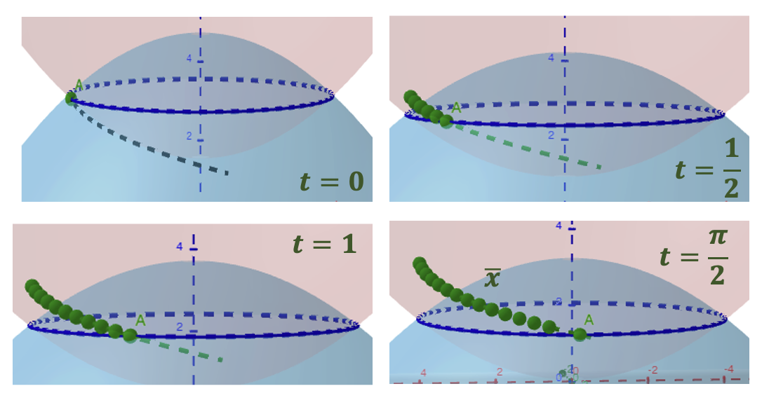
Figure 1: Example 6.1

Consider the problem $(P)$ with the following data $($see Figure 1$)$.

• The perturbation mappings $f\colon[0,\frac{\pi}{2}]\times\mathbb{R}^{3}\times\mathbb{R}\times\mathbb{R}\longrightarrow\mathbb{R}^{3}$ and $g\colon[0,\frac{\pi}{2}]\times\mathbb{R}^{3}\times\mathbb{R}\times\mathbb{R}\longrightarrow\mathbb{R}$ are defined by

  $$f\left(t,(x_{1},x_{2},x_{3}),y,u\right)=(x_{1}-x_{2}-u+y^{2},x_{1}+x_{2}+u+y^{3},x_{3}+t-\pi-1);$$

  $$g\left(t,(x_{1},x_{2},x_{3}),y,u\right)=x_{1}^{2}+x_{2}^{2}-16+u+y.$$

• The two functions $\psi_{1},\;\psi_{2}\colon[0,\frac{\pi}{2}]\times\mathbb{R}^{3}\longrightarrow\mathbb{R}$ are defined by

  $$\psi_{1}(t,x_{1},x_{2},x_{3})\mathrel{\mathop{\mathchar 58\relax}}=x_{1}^{2}+x_{2}^{2}+\frac{32}{\pi}x_{3}+\frac{32}{\pi}t-48,\;\;\psi_{2}(t,x_{1},x_{2},x_{3})\mathrel{\mathop{\mathchar 58\relax}}=x_{1}^{2}+x_{2}^{2}-\frac{32}{\pi}x_{3}-\frac{32}{\pi}t+16,$$

  and hence, for each $t\in[0,\frac{\pi}{2}]$, the set $C(t)$ is the nonsmooth, convex and bounded set

  $$C(t) = C_{1}(t)\cap C_{2}(t)$$

  $$\mathrel{\mathop{\mathchar 58\relax}}= \{(x_{1},x_{2},x_{3})\mathrel{\mathop{\mathchar 58\relax}}\psi_{1}(t,x_{1},x_{2},x_{3})\leq 0\}\cap\{(x_{1},x_{2},x_{3})\mathrel{\mathop{\mathchar 58\relax}}\psi_{2}(t,x_{1},x_{2},x_{3})\leq 0\}.$$

• The objective function ${J}\colon\mathbb{R}^{8}\longrightarrow\mathbb{R}\cup\{\infty\}$ is defined by

  $$J(x_{1},x_{2},x_{3},y_{1},x_{4},x_{5},x_{6},y_{2})\mathrel{\mathop{\mathchar 58\relax}}=\begin{cases}-x_{4}^{2}-x_{5}^{2}+16+\mathinner{\!\left\lvert\frac{\pi}{2}-x_{6}\right\rvert}&\;\;(x_{4},x_{5},x_{6})\in C(\frac{\pi}{2}),\vspace{0.1cm}\\ \infty&\;\;\hbox{Otherwise}.\end{cases}$$

• The control multifunction is the constant $U(t)\mathrel{\mathop{\mathchar 58\relax}}=[0,1]$ for all $t\in[0,\frac{\pi}{2}]$.

• The set $S$ is given by

  $$S\mathrel{\mathop{\mathchar 58\relax}}=\{(x_{1},x_{2},x_{3},y_{1},x_{4},x_{5},x_{6},y_{2})\in\mathbb{R}^{8}\mathrel{\mathop{\mathchar 58\relax}}x_{1}^{2}+x_{2}^{2}=16,x_{3}=\pi,x_{2}+x_{6}^{2}=\frac{\pi^{2}}{4},$$

  $$\frac{x_{1}^{2}}{8}+x_{4}=2,y_{1}+x_{2}^{2}=0\}.$$

Define, for each $t\in[0,\frac{\pi}{2}]$, the curve

$$\Gamma(t)\mathrel{\mathop{\mathchar 58\relax}}=\left\{(x_{1},x_{2},x_{3})\mathrel{\mathop{\mathchar 58\relax}}x_{1}^{2}+x_{2}^{2}=16\;\hbox{and}\;x_{3}=\pi-t\right\}=\left(\textnormal{bdry}\,C_{1}(t)\cap\textnormal{bdry}\,C_{2}(t)\right)\subset\textnormal{bdry}\,C(t).$$

Since $S\subset\Gamma(0)\times\mathbb{R}\times\mathbb{R}^{3}\times\mathbb{R}$ and ${J}$ vanishes on $\mathbb{R}^{3}\times\mathbb{R}\times\Gamma(\frac{\pi}{2})\times\mathbb{R}$ and is strictly positive elsewhere in $\mathbb{R}^{3}\times\mathbb{R}\times C(\frac{\pi}{2})\times\mathbb{R}$, we may seek for $(P)$ a candidate $((\bar{x},\bar{y}),\bar{u})$ for optimality with $\bar{x}(t)\mathrel{\mathop{\mathchar 58\relax}}=(\bar{x}_{1}(t),\bar{x}_{2}(t),\bar{x}_{3}(t))$ belonging to $\Gamma(t)$ for every $t$, if possible, and hence we have

$$\begin{cases}\bar{x}_{1}^{2}(t)+\bar{x}_{2}^{2}(t)=16\;\,\hbox{and}\,\;\bar{x}_{3}(t)=\pi-t\;\forall t\in[0,\tfrac{\pi}{2}]\,\;\hbox{and}\\[1.0pt] \bar{x}_{1}(t)\dot{\bar{x}}_{1}(t)+\bar{x}_{2}(t)\dot{\bar{x}}_{2}(t)=0\text{ a.e. }\,\;\hbox{and}\\[1.0pt] (\bar{x}(0)^{\mkern-1.5mu\mathsf{T}},\bar{y}(0)^{\mkern-1.5mu\mathsf{T}},\bar{x}(\tfrac{\pi}{2})^{\mkern-1.5mu\mathsf{T}},\bar{y}(\tfrac{\pi}{2})^{\mkern-1.5mu\mathsf{T}})\in\{(4,0,\pi,0,0,4,\frac{\pi}{2},a),(-4,0,\pi,0,0,4,\frac{\pi}{2},b),\\[1.0pt] \;\;\;\;\;\;\;\;\;\;\;\;\;\;\;\;\;\;(4,0,\pi,0,0,-4,\frac{\pi}{2},c),(-4,0,\pi,0,0,-4,\frac{\pi}{2},d);\;a,b,c,d\in\mathbb{R}\}.\end{cases}$$ (132)

One can readily verify that all assumptions of Theorem 2.1 are satisfied for any choice of $(\bar{x},\bar{y})$ such that $\bar{x}(t)\in\Gamma(t)$ for all $t$, with $(A3.3)$ being satisfied for $\beta=(1,1)$. Applying Theorem 2.1 to such candidate $((\bar{x},\bar{y}),\bar{u})$ we obtain the existence of an adjoint vector $p=(q,v)$ where $q\mathrel{\mathop{\mathchar 58\relax}}=(q_{1},q_{2},q_{3})\in BV([0,\frac{\pi}{2}];\mathbb{R}^{3})$, $v\in W^{1,1}([0,\frac{\pi}{2}];\mathbb{R})$, two finite signed Radon measures $\nu_{1}$, $\nu_{2}$ on $\left[0,\frac{\pi}{2}\right]$, $\xi_{1}$, $\xi_{2}\in L^{\infty}([0,\tfrac{\pi}{2}];\mathbb{R}^{+})$, and $\lambda\geq 0$, such that when incorporating equations (132) into Theorem 2.1$(i)$-$(vii)$, we obtain

1. $\|p(\frac{\pi}{2})\|+\lambda=1.$

2. The admissibility equation holds, that is, for $t\in[0,\tfrac{1}{2}]$ a.e.,

   $$\begin{cases}\dot{\bar{x}}_{1}(t)=\bar{x}_{1}(t)-\bar{x}_{2}(t)-\bar{u}(t)+\bar{y}^{2}(t)-2\bar{x}_{1}(t)(\xi_{1}(t)+\xi_{2}(t)),\\ \dot{\bar{x}}_{2}(t)=\bar{x}_{1}(t)+\bar{x}_{2}(t)+\bar{u}(t)+\bar{y}^{3}(t)-2\bar{x}_{2}(t)(\xi_{1}(t)+\xi_{2}(t)),\\ \dot{\bar{x}}_{3}(t)=\bar{x}_{3}(t)+t-\pi-1-\frac{32}{\pi}(\xi_{1}(t)-\xi_{2}(t)),\\ \dot{\bar{y}}(t)=\bar{x}_{1}^{2}(t)+\bar{x}_{2}^{2}(t)-16+\bar{u}(t)+\bar{y}(t).\end{cases}$$

3. The adjoint equation is satisfied, that is, for $t\in[0,\frac{\pi}{2}]$,

   $$dq(t) = \begin{pmatrix}\begin{array}[]{rrr}-1&-1&0\\ 1&-1&0\\ 0&0&-1\end{array}\end{pmatrix}q(t)\;dt\;+\begin{pmatrix}-2\bar{x}_{1}(t)\\ -2\bar{x}_{2}(t)\\ 0\end{pmatrix}v(t)dt\;$$

   $$+ (\xi_{1}(t)+\xi_{2}(t))\begin{pmatrix}2\;\;&0\;\;&0\\ 0\;\;&2\;\;&0\\ 0\;\;&0\;\;&0\end{pmatrix}q(t)\;dt\;+\;\begin{pmatrix}2\bar{x}_{1}(t)\\ 2\bar{x}_{2}(t)\\ \frac{32}{\pi}\end{pmatrix}d\nu_{1}+\begin{pmatrix}2\bar{x}_{1}(t)\\ 2\bar{x}_{2}(t)\\ -\frac{32}{\pi}\end{pmatrix}d\nu_{2},$$

   $$\dot{v}(t) = \begin{pmatrix}\begin{array}[]{rrr}0&0&0\\ \end{array}\end{pmatrix}q(t)\;dt\;-v(t)$$

4. The complementary slackness condition is valid, that is, for $t\in[0,\tfrac{\pi}{2}]$ a.e.,

   $$\begin{cases}\xi_{1}(t)(2q_{1}(t)\bar{x}_{1}(t)+2q_{2}(t)\bar{x}_{2}(t)+\frac{32}{\pi}q_{3}(t))=0,\\ \xi_{2}(t)(2q_{1}(t)\bar{x}_{1}(t)+2q_{2}(t)\bar{x}_{2}(t)-\frac{32}{\pi}q_{3}(t))=0.\end{cases}$$

5. The transversality condition holds, that is,

   $$(q(0),v(0),-q(\frac{\pi}{2}),-v(\frac{\pi}{2}))^{\mkern-1.5mu\mathsf{T}}\in\lambda\{(0,0,0,0,0,-8,\alpha,0)\mathrel{\mathop{\mathchar 58\relax}}\alpha\in[-1,1]\}$$

   $$+\{(8\alpha_{1}+\alpha_{4},\alpha_{3},\alpha_{2},\alpha_{5},\alpha_{4},0,\alpha_{3}\pi,0)\mathrel{\mathop{\mathchar 58\relax}}\alpha_{1},\alpha_{2},\alpha_{3},\alpha_{4},\alpha_{5}\in\mathbb{R}\}$$

   $$\hbox{if}\;\;(\bar{x}(0)^{\mkern-1.5mu\mathsf{T}},\bar{y}(0)^{\mkern-1.5mu\mathsf{T}},\bar{x}(\tfrac{\pi}{2})^{\mkern-1.5mu\mathsf{T}},\bar{y}(\tfrac{\pi}{2})^{\mkern-1.5mu\mathsf{T}})\in\{(4,0,\pi,0,0,4,\frac{\pi}{2},a)\mathrel{\mathop{\mathchar 58\relax}}a\in\mathbb{R}\}.$$

   Similarly, we work on deriving transversality conditions for each of the four cases in (132).

6. $\max\{u\;(-q_{1}(t)+q_{2}(t)+v(t))\mathrel{\mathop{\mathchar 58\relax}}u\in[0,1]\}$ is attained at $\bar{u}(t)$ for $t\in[0,\frac{\pi}{2}]$ a.e.

We temporarily assume that

$$-q_{1}(t)+q_{2}(t)+v(t)<0,\;\;\forall t\in[0,\tfrac{\pi}{2}]\;\hbox{a.e.}$$ (133)

This gives from (f) that $\bar{u}(t)=0$ for $t\in[0,\frac{\pi}{2}]$ a.e. Now solving the differential equations of (b) and using (132), we obtain that

$$\xi_{1}(t)=\xi_{2}(t)=\frac{1}{4},\;\,\bar{x}(t)^{\mkern-1.5mu\mathsf{T}}=(4\cos t,4\sin t,\pi-t),\;\;\hbox{and}\;\;\bar{y}(t)=0\;\;\forall t\in[0,\tfrac{\pi}{2}].$$

Hence, from (d), we deduce that $q_{3}(t)=0$ for $t\in[0,\frac{\pi}{2}]$ a.e., and

$$\cos t\;q_{1}(t)+\sin t\;q_{2}(t)=0,\;\,\forall t\in[0,\tfrac{\pi}{2}]\;\textnormal{a.e.},$$ (134)

and the adjoint equation (c) simplifies to the following

$$\begin{cases}\dot{v}(t)=-v(t),\\ d{q}_{1}(t)=(-q_{1}(t)-q_{2}(t))dt-8\cos t\;v(t)dt+q_{1}(t)\;dt+8\cos t\;(d\nu_{1}+d\nu_{2}),\\ d{q}_{2}(t)=(q_{1}(t)-q_{2}(t))dt-8\sin t\;v(t)dt+q_{2}(t)\;dt+8\sin t\;(d\nu_{1}+d\nu_{2}),\\ d{{q}}_{3}(t)=-q_{3}(t)\;dt+\frac{32}{\pi}(d\nu_{1}-d\nu_{2}).\end{cases}$$ (135)

Since $v(\frac{\pi}{2})=0$ then $v(t)=0\;\forall t\in[0,\frac{\pi}{2}]$. Using (a), (134), (e), and (135), one can get the following

$$\begin{cases}\lambda=\tfrac{2\pi}{2\pi+\sqrt{1+(16\pi)^{2}}}\;\,\hbox{and}\;\,A=\tfrac{1}{2\pi+\sqrt{1+(16\pi)^{2}}},\\[2.0pt] q(t)^{\mkern-1.5mu\mathsf{T}}=\left(A\sin t,-A\cos t,0\right)\;\hbox{on}\;[0,\tfrac{\pi}{2}),\;\;\quad q(\tfrac{\pi}{2})^{\mkern-1.5mu\mathsf{T}}=(A,16A\pi,0),\\[2.0pt] d\nu_{1}=d\nu_{2}=A\pi\delta_{\big{\{}\tfrac{\pi}{2}\big{\}}},\end{cases}\vspace{0.01cm}$$

where $\delta_{\{a\}}$ denotes the unit measure concentrated on the point $a$. Note that for all $t\in[0,\tfrac{\pi}{2}]$, we have $-q_{1}(t)+q_{3}(t)+v(t)<0$, and hence, the temporary assumption (133) is satisfied.
Therefore, the above analysis, realized via Theorem 2.1, produces an admissible pair $((\bar{x},\bar{y}),\bar{u})$, where

$$\textstyle\bar{x}(t)^{\mkern-1.5mu\mathsf{T}}=(4\cos t,4\sin t,\pi-t),\;\;\bar{y}(t)=0,\;\;\hbox{and}\;\;\bar{u}(t)=0,\;\;\forall t\in[0,\tfrac{\pi}{2}],$$

which is optimal for $(P)$.

7. Appendix

The following result holds for uniform prox-regular sets $S(t)$ not necessarily being sublevel sets. It is an extension of a special case of [41, Lemma 3.2] from a constant compact set $S$ to the case of set-valued maps $S(\cdot)$ with non-compact values. It requires $N_{S(\cdot)}(\cdot)$ to have closed graph.

Lemma 7.1.

Let $S(\cdot)\mathrel{\mathop{\mathchar 58\relax}}[0,T]\rightsquigarrow\mathbb{R}^{n}$ be such that, for all $t\in[0,T]$, $S(t)$ is nonempty, closed, and uniformly $\rho^{*}$-prox-regular, for some $\rho^{*}>0$. Let $\bar{x}\in\mathcal{C}([0,T],\mathbb{R}^{n})$ with $\bar{x}(t)\in S(t)$ for all $t\in[0,T]$. Assume that for some $\delta\in(0,\rho^{*})$, the map $(t,y)\to N_{S(t)}(y)$ has closed graph on the domain Gr $\left(S(\cdot)\cap\bar{B}_{\delta}(\bar{x}(\cdot))\right)$.Then, the following holds.

• There exists ${\rho}_{\delta}>0$ such that for all $t\in[0,T]$ the set $S(t)\cap\bar{B}_{\delta}(\bar{x}(t))$ is ${\rho}_{\delta}$-prox-regular.

• For $t\in[0,T]$, $\pi(t,\cdot)\mathrel{\mathop{\mathchar 58\relax}}=\pi_{\left(S(t)\cap\bar{B}_{\delta}(\bar{x}(t))\right)}(\cdot)$ is well-defined on $\left(S(t)\cap\bar{B}_{\delta}(\bar{x}(t))\right)+{\rho}_{\delta}B$ and $2$-lipschitz on $\left(S(t)\cap\bar{B}_{\delta}(\bar{x}(t))\right)+\frac{{\rho}_{\delta}}{2}\bar{B}$.

Proof.

$(i)$: The result is derived by following the proof of [41, Lemma 3.2], where for $t\in[0,T]$, we take $S\mathrel{\mathop{\mathchar 58\relax}}=S(t)$ and $x\mathrel{\mathop{\mathchar 58\relax}}=\bar{x}(t)$, and hence, $\mathcal{N}_{x}$ and $\rho_{x}$ there , are respectively $\mathcal{N}_{t}\mathrel{\mathop{\mathchar 58\relax}}=\mathcal{N}_{\bar{x}(t)}$ and $\rho_{t}\mathrel{\mathop{\mathchar 58\relax}}=\rho_{\bar{x}(t)}$. It follows that $\rho$ there is now $\hat{\rho}\mathrel{\mathop{\mathchar 58\relax}}=\inf\{\rho_{t}\mathrel{\mathop{\mathchar 58\relax}}t\in[0,T]\}$. Following the rest of the proof there, and employing that the map $(t,y)\to N_{S(t)}(y)$ has closed graph on the domain Gr $\left(S(\cdot)\cap\bar{B}_{\delta}(\bar{x}(\cdot))\right)$, we conclude that $\hat{\rho}>0$. Thus, for all $t\in[0,T]$, we deduce that $S(t)\cap\bar{B}_{\delta}(\bar{x}(t))$ is $\rho_{\delta}$-prox regular, where $\rho_{\delta}\mathrel{\mathop{\mathchar 58\relax}}=\frac{\rho^{*}\hat{\rho}}{2}$.
$(ii)$: It follows from $(i)$ and [17, Theorem 4.8]. ∎

Translating Lemma 6.2 in [43] to our setting gives us the following lemma.

Lemma 7.2.

Assume that $\psi_{i}$ is continuous for all $i=1,\dots,r$. Let $\alpha_{n}\geq 0$, for all $n\in\mathbb{N}$, with $\alpha_{n}\longrightarrow\alpha_{o}$ and let $(t_{n},c_{n})\in$ Gr $C(\cdot)$ be a sequence such that $\mathcal{I}^{\alpha_{n}}_{(t_{n},c_{n})}\neq\emptyset$, for all $n\in\mathbb{N}$, and $(t_{n},c_{n})\longrightarrow(t_{o},c_{o})$. Then, $\mathcal{I}^{\alpha_{o}}_{(t_{o},c_{o})}\neq\emptyset$ and there exist $\emptyset\not=\mathcal{J}_{o}\subset\{1,\dots,r\}$ and a subsequence of $(\alpha_{n},t_{n},c_{n})_{n}$ we do not relabel, such that

$$\mathcal{I}^{\alpha_{n}}_{(t_{n},c_{n})}=\mathcal{J}_{o}\subset\mathcal{I}^{\alpha_{o}}_{(t_{o},c_{o})}\;\,\hbox{for all}\;\,n\in\mathbb{N}.$$

In particular, for all $a\geq 0$, for any continuous function $x\colon[0,T]\longrightarrow\mathbb{R}^{n}$ such that $x(t)\in C(t)$ for all $t\in[0,T]$, we have $I^{a}(x)$ is closed, and hence compact.

This result shall be used in different places of this paper.

Lemma 7.3.

(i). Let $(x_{n},y_{n})\in W^{1,\infty}([0,T];\mathbb{R}^{n+d})$, $(\xi_{n}^{1},\cdots,\xi_{n}^{\mathcal{R}},\zeta_{n})\in L^{\infty}([0,T],\mathbb{R}_{+}^{\mathcal{R}+1})$,   be such that, for some positive constants $M_{1},M_{2},M_{3}$ we have, $\forall n\in\mathbb{N}$ and $\forall i\in\{1,\cdots,\mathcal{R}\},$

$$\|(x_{n},y_{n})\|_{\infty}\leq M_{1},\;\;\|(\dot{x}_{n},\dot{y}_{n})\|_{\infty}\leq M_{2},\;\;\|(\xi^{i}_{n},\zeta_{n})\|_{\infty}\leq M_{3}.$$ (136)

Then, there exist $(x,y)\in W^{1,\infty}([0,T];\mathbb{R}^{n+d})$ and $(\xi^{1},\cdots,\xi^{\mathcal{R}},\zeta)\in L^{\infty}([0,T];\mathbb{R}^{\mathcal{R}+1}_{+})$ such that $(x_{n},y_{n})$, and $(\xi_{n}^{1},\cdots,\xi_{n}^{\mathcal{R}},\zeta_{n})$ admit a subsequence $($not relabeled$)$ satisfying $\forall i\in\{1,\cdots,\mathcal{R}\},$

$$\begin{cases}(x_{n},y_{n})\xrightarrow[]{unif}(x,y),\quad(\dot{x}_{n},\dot{y}_{n})\xrightarrow[in\;L^{\infty}]{w*}(\dot{x},\dot{y}),\;\;(\xi^{i}_{n},\zeta_{n})\xrightarrow[in\;L^{\infty}]{w*}(\xi^{i},\zeta),\\ \|(x,y)\|_{\infty}\leq M_{1},\;\;\|(\dot{x},\dot{y})\|_{\infty}\leq M_{2},\;\;\|(\xi^{i},\zeta)\|_{\infty}\leq M_{3}.\end{cases}$$ (137)

(ii). For given $q_{i}\mathrel{\mathop{\mathchar 58\relax}}[0,T]\times\mathbb{R}^{n}\longrightarrow\mathbb{R}$, let $Q(t)\mathrel{\mathop{\mathchar 58\relax}}=\cap_{i=1}^{\mathcal{R}}\{x\in\mathbb{R}^{n}\mathrel{\mathop{\mathchar 58\relax}}q_{i}(t,x)\leq 0\}$ and $(\bar{x},\bar{y})\in\mathcal{C}([0,T];\mathbb{R}^{n}\times\mathbb{R}^{l})$ be such that $\bar{x}(t)\in Q(t)\;\forall t\in[0,T]$. Assume $(A2)$ is satisfied by $C(t)\mathrel{\mathop{\mathchar 58\relax}}=Q(t)$, and, for some $\bar{\delta}\,>0$, $(A3.1)$ and $(A4.1)$ hold at $((\bar{x},\bar{y});\bar{\delta})$ respectively by $\psi_{i}\mathrel{\mathop{\mathchar 58\relax}}=q_{i}$ and $h=(f,g)\mathrel{\mathop{\mathchar 58\relax}}[0,T]\times\mathbb{R}^{n}\times\mathbb{R}^{l}\times\mathbb{R}^{m}\longrightarrow\mathbb{R}^{n}\times\mathbb{R}^{l}.$ Let $(x_{n},y_{n})$ and $(\xi_{n},\cdots,\xi_{n}^{\mathcal{R}},\zeta_{n})$ be such that $(x_{n}(t),y_{n}(t))\in[Q(t)\cap\bar{B}_{\bar{\delta}}(\bar{x}(t))]\times\bar{B}_{\bar{\delta}}(\bar{y}(t))\,(\forall t\in[0,T])$ and (136) is satisfied, and let $(x,y,\xi^{i},\zeta)$ be their corresponding limits via (137). Consider $u_{n}\in\mathcal{U}$ such that, for all $n\in\mathbb{N}$, $((x_{n},y_{n}),u_{n})$, and $(\xi_{n}^{1},\cdots,\xi_{n}^{\mathcal{R}},\zeta_{n})$ satisfy

$$\begin{cases}\dot{x}(t)=f(t,x(t),y(t),u(t))-\sum_{i=1}^{\mathcal{R}}\xi^{i}(t)\nabla_{x}q_{i}(t,x(t))\text{ a.e. }t\in[0,T],\\ \dot{y}(t)=g(t,x(t),y(t),u(t))-\zeta(t)\nabla_{y}\varphi(t,y(t))\text{ a.e. }t\in[0,T],\end{cases}$$ (138)

where $\varphi$ is given by (14).Then, in either of the following cases, there exists $u\in\mathcal{U}$ such that $((x,y),u)$, and $(\xi^{1},\cdots,\xi^{\mathcal{R}},\zeta)$ also satisfy system (138).
Case 1. If there exists a subsequence of $u_{n}$ that converges pointwise a.e. to some $u\in\mathcal{U}$.
Case 2. If $(A1)$ and $(A4.2)$ are satisfied.

Proof.

(i): By (136), the sequence $(x_{n},y_{n})_{n}$ is equicontinuous and uniformly bounded. Hence, using Arzela-Ascoli theorem and that $(\dot{x}_{n},\dot{y}_{n})$ is uniformly bounded in $L^{\infty}$, it follows that there exists $(x,y)\in W^{1,\infty}([0,T];\mathbb{R}^{n+d})$ such that along a subsequence (we do not relabel) of $(x_{n},y_{n})$, we have $(x_{n},y_{n})\xrightarrow[]{unif}(x,y)$, $(\dot{x}_{n},\dot{y}_{n})\xrightarrow[in\;L^{\infty}]{w*}(\dot{x},\dot{y})$, with $(x,y)$ and $(\dot{x},\dot{y})$ satisfy the bounds in (137). As $\|(\xi^{i}_{n},\zeta_{n})\|_{\infty}\leq M_{3}$ for all $i=1,\cdots,\mathcal{R}$ and for all $n\in\mathbb{N}$, some subsequences of $(\xi_{n}^{1},\cdots,\xi_{n}^{\mathcal{R}},\zeta_{n})$ converge in the weak^∗-topology to some $(\xi^{1},\cdots,\xi^{\mathcal{R}},\zeta)\in L^{\infty}$ which satisfy the required bound in (137).

(ii) Case 1: Let $t\in[0,T)$ lebesgue point of $\dot{x}(\cdot),\dot{y}(\cdot),f(\cdot,x(\cdot),y(\cdot),u(\cdot)),G(\cdot,x(\cdot),y(\cdot),u(\cdot))$, $\xi^{i}(\cdot)$ for all $i=1,\cdots,\mathcal{R}$ and $\zeta$, and let $\tau\in(0,T-t)$. Then, (138) implies

$$\begin{cases}\frac{x_{n}(t+\tau)-x_{n}(t)}{\tau}=\frac{1}{\tau}\int_{t}^{t+\tau}\left[f(s,x_{n}(s),y_{n}(s),u_{n}(s))-\sum_{i=1}^{\mathcal{R}}\xi_{n}^{i}(s)\nabla_{x}q_{i}(s,x_{n}(s))\right]ds,\\ \frac{y_{n}(t+\tau)-y_{n}(t)}{\tau}=\frac{1}{\tau}\int_{t}^{t+\tau}\left[g(s,x_{n}(s),y_{n}(s),u_{n}(s))-\zeta_{n}(s)\nabla_{y}\varphi(s,y_{n}(s))\right]ds.\end{cases}$$ (139)

Using Dominated Convergence Theorem, and taking the limit as $n\rightarrow\infty$ of (139), we deduce that

$$\begin{cases}\frac{x(t+\tau)-x(t)}{\tau}=\frac{1}{\tau}\int_{t}^{t+\tau}[f(s,x(s),y(s),u(s))-\sum_{i=1}^{\mathcal{R}}\xi^{i}(s)\nabla_{x}q_{i}(s,x(s))]ds,\\ \frac{y(t+\tau)-y(t)}{\tau}=\frac{1}{\tau}\int_{t}^{t+\tau}\left[g(s,x(s),y(s),u(s))-\zeta(s)\nabla_{y}\varphi(s,y(s))\right]ds.\end{cases}$$ (140)

Now, let $\tau\to 0$ in $(\ref{xeq})$, we get that (138) is satisfied for every $t$ lebesgue point, hence it hold for a.e. $t\in[0,T]$.
(ii) Case 2: For $s\in[0,T]$ a.e., define in $\mathbb{R}^{n}\times\mathbb{R}^{l}$ the sets $S_{n}(s)\mathrel{\mathop{\mathchar 58\relax}}=h(s,x_{n}(s),y_{n}(s),U(s))$ and $S(s)\mathrel{\mathop{\mathchar 58\relax}}=h(s,x(s),y(s),U(s))$. Using (A1), the continuity of $h(s,\cdot,\cdot,\cdot)$ in (A4.1), and the convexity assumption (A4.2), it follows that $S_{n}(s)$ and $S(s)$ are nonempty closed convex sets and $S_{n}(s)$ Hausdorff-converges to $S(s)$. Hence, Filippov Selection Theorem yields that $((x_{n},y_{n}),u_{n})$ and $(\xi^{i}_{n},\zeta_{n})$ satisfying (138) is equivalent to, $\forall z\in\mathbb{R}^{n+d}$ and $s\in[0,T]$ a.e.,

$$\langle z,(\dot{x}_{n}(s),\dot{y}_{n}(s))\rangle\leq \sigma(z,h(s,x_{n}(s),y_{n}(s),U(s)))$$ (141)

$$-\langle z,(\sum_{i=1}^{\mathcal{R}}\xi_{n}^{i}(s)\nabla_{x}q_{i}(t,x_{n}(s)),\zeta_{n}(s)\nabla_{y}\varphi(s,y_{n}(s)))\rangle.$$

Furthermore, by $\eqref{limitsetconvergence}$ and the positive homogeneity of $\sigma(\cdot,S_{n})$ and $\sigma(\cdot,S),$ we deduce that

$$\sigma(z,h(s,x_{n}(s),y_{n}(s),U(s)))\xrightarrow[k\to\infty]{}\sigma(z,h(s,x(s),y(s),U(s))),\,\forall z\in\mathbb{R}^{n+d}\,\mbox{and }\;s\in[0,T]\;\mbox{a.e.},$$

and the bound of $h$ in (A4.1) gives that, for $z\in\mathbb{R}^{n+d}$,

$$|\sigma\left(z,h(s,x_{n}(s),y_{n}(s),U(s))\right)| \leq 2\|z\|M_{h}.$$

Thus, for $t\in[0,T)$ a lebesgue point of $\xi^{i}(\cdot),\zeta(\cdot),\dot{x}(\cdot),\dot{y}(\cdot),\sigma(z,h(\cdot,x(\cdot),y(\cdot),U(\cdot)))$, and for $\tau\in(0,T-t)$, when integrating $(\ref{ineqk})$ on $[t,t+\tau]$ and then taking the limit as $n\to\infty$, the Dominated Convergence Theorem yields that, $\forall z=(z_{1},z_{2})\in\mathbb{R}^{n}\times\mathbb{R}^{l}$,

$$\int_{t}^{t+\tau}\langle z,(\dot{x}(s),\dot{y}(s))\rangle ds$$

$$\leq \int_{t}^{t+\tau}[\sigma(z,h(s,x(s),y(s),U(s)))-\langle z,(\sum_{i=1}^{\mathcal{R}}\xi^{i}(s)\nabla_{x}q_{i}(s,x(s)),\zeta(s)\nabla_{y}\varphi(s,y(s)))\rangle]ds.$$

Dividing the last equation by $\tau$ and taking the limit when $\tau\to 0$, we get that, $\forall z\in\mathbb{R}^{n}\times\mathbb{R}^{l},$ and for $t$ lebesgue point,

$$\langle z,(\dot{x}(t),\dot{y}(t))\rangle\leq\sigma(z,h(t,x(t),y(t),U(t)))-\langle z,(\sum_{i=1}^{\mathcal{R}}\xi^{i}(t)\nabla_{x}q_{i}(t,x(t)),\zeta(t)\nabla_{y}\varphi(t,y(t)))\rangle,$$

and hence this inequality is valid for $t\in[0,T]$ a.e. Therefore, by means of Filipov Selection Theorem, there exists $u\in\mathcal{U}$, such that $((x,y),u)$, and $(\xi^{1},\cdots,\xi^{\mathcal{R}},\zeta)$ satisfy system (138). ∎

Remark 7.4.

When $\bar{\delta}=\infty$, Lemma 7.3 remains valid with $(\bar{x},\bar{y})$ and the assumptions involving them are now superfluous. In this case, recall that $(A3.1)$,$(A4.1)$, and $(A4.2)$ are replaced by $(A3.1)_{G}$, $(A4.1)_{G}$, and $(A4.2)_{G}$, respectively.

References

- [1] L. Adam, J. Outrata, On Optimal Control of a Sweeping Process Coupled with an Ordinary Differential Equation, Discrete Contin. Dyn. Syst. B 19, 2709–2738 (2014)
- [2] S. Adly, F. Nacry, L. Thibault, Discontinuous sweeping process with prox-regular sets, ESAIM COCV, 23/4 1293–1329 (2017).
- [3] A. Bensoussan, K. Chandrasekaran , J. Turi J., Optimal Control of Variational Inequalities, Commun. Inf. Syst. Vol. 10 No.4, 203–220 (2010)
- [4] A. Bergqvist, Magnetic Vector Hysteresis Model with Dry Friction-like Pinning, Phys. B Condens. Matter Vol. 233, No. 4, 342–347 (1997)
- [5] A. Bouach, T. Haddad, B.S. Mordukhovich, Optimal Control of Nonconvex Integro-differential Sweeping Processes, J. Differ. Equ. Vol. 329, 255–317 (2022)
- [6] M. Brokate, P. Krejčí, Optimal Control of ODE Systems Involving a Rate Independent Variational Inequality, Discrete and continuous dynamical systems series B 18, 331–348 (2013)
- [7] M. Brokate, J. Sprekels, Hysteresis and Phase Transitions, Volume 121. Springer New York, (1996)
- [8] T.H. Cao, B.S. Mordukhovich, D. Nguyen, T. Nguyen, Applications of Controlled Sweeping Processes to Nonlinear Crowd Motion Models with Obstacles, IEEE Control Systems Letters Vol 6 740-745 (2021)
- [9] T.H. Cao, G. Colombo, B. Mordukhovich, D. Nguyen, Optimization of Fully Controlled Sweeping Processes, Journal of Differential Equations 295 138–186 (2021)
- [10] T.H. Cao, G. Colombo, B. Mordukhovich, D. Nguyen, Optimization and discrete approximation of sweeping processes with controlled moving sets and perturbations, Journal of Differential Equations 274 461–509 (2021)
- [11] T.H. Cao, B. Mordukhovich, Optimality conditions for a controlled sweeping process with applications to the crowd motion model, Disc. Cont. Dyn. Syst. Ser. B 22, 267–306 (2017)
- [12] T.H. Cao, B. Mordukhovich, Optimal control of a nonconvex perturbed sweeping process, Journal of Differential Equations 266, 1003–1050 (2019)
- [13] C. Castaing, A. Salvadori, L. Thibault, Functional evolution equations governed by nonconvex sweeping Process, J. Nonlinear Conv. Anal. 2, 217–241 (2001)
- [14] F.H. Clarke, Optimization and Nonsmooth Analysis, John Wiley, New York (1983)
- [15] F.H. Clarke, Functional Analysis, Calculus of Variations and Optimal Control, Graduate Texts in Mathematics, 264. Springer, London (2013)
- [16] F.H. Clarke, Yu. Ledyaev, R.J. Stern, P.R. Wolenski, Nonsmooth Analysis and Control Theory, Graduate Texts in Mathematics, 178, Springer-Verlag, New York (1998)
- [17] F.H. Clarke, R.J. Stern, P.R. Wolenski, Proximal smoothness and the lower- property, J. Convex Analysis 2, 117–144 (1995)
- [18] G. Colombo, P. Godini, On the optimal control of rate-independent soft crawlers, Journal de Mathématiques Pures et Appliquées (2020)
- [19] G. Colombo, R. Henrion, N.D. Hoang, B.S. Mordukhovich, Optimal control of the sweeping process, Dyn. Contin. Discrete Impuls. Syst. Ser. B 19, 117–159 (2012)
- [20] G. Colombo, R. Henrion, N.D. Hoang, B.S. Mordukhovich, Optimal control of the sweeping process over polyhedral controlled sets, Journal of Differential Equations 260 no. 4, 3397–3447 (2016)
- [21] Colombo G., Mordukhovich B., Nguyen D.: Optimal Control of Sweeping Processes in Robotics and Traffic Flow Models, J. Optim. Theory Appl. Vol. 182 No. 2, 439–472 (2019)
- [22] G. Colombo, B. Mordukhovich,D. Nguyen, Optimization of a perturbed sweeping process by constrained discontinuous controls, SIAM Journal on Control and Optimization, 58 no. 4, 2678–2709 (2020)
- [23] M.d.R. de Pinho, M.M.A. Ferreira, G.V. Smirnov, Optimal Control Involving Sweeping Processes, Set-Valued Var. Anal. 27, no. 2, 523–548 (2019)
- [24] M.d.R. de Pinho, M.M.A. Ferreira, G.V. Smirnov, Correction to: Optimal Control Involving Sweeping Processes, Set-Valued Var. Anal. 27, 1025–1027 (2019)
- [25] M.d.R. de Pinho, M.M.A. Ferreira, G.V. Smirnov, Optimal Control with Sweeping Processes: Numerical Method, J Optim Theory Appl 185, 845–858 (2020)
- [26] M.d.R. de Pinho, M.M.A. Ferreira, G.V. Smirnov, Necessary conditions for optimal control problems with sweeping systems and end point constraints, Optimization,, 71:11, 3363–3381 (2021)
- [27] M.d.R. de Pinho, M.M.A. Ferreira, G.V. Smirnov, A Maximum Principle for Optimal Control Problems involving Sweeping Processes with a Nonsmooth Set, J Optim Theory Appl 199, 273-297 (2023)
- [28] J.F. Edmond, L. Thibault, Relaxation of an optimal control problem involving a perturbed sweeping process, Mathematical programming - Series B, 104, 347–373 (2005)
- [29] J.K. Hale, Ordinary differential equations, second edition, Krieger Publishing Company (1980)
- [30] J.M. Harrison, M.I. Reiman, Reflected Brownian motion on an orthant, Ann. Probab. 9, 302–308 (1981)
- [31] C. Hermosilla, M. Palladino, Optimal Control of the Sweeping Process with a Nonsmooth Moving Set, SIAM Journal on Control and Optimization, 60:5, 2811–2834 (2022)
- [32] J.-B. Hiriart-Urruty, Extension of Lipschitz functions, J. Math. Anal. Appl. 77, 539–554 (1980)
- [33] B. Li, Generalizations of Diagonal Dominance in Matrix Theory, Ph.D Thesis, Saskatchewan, Regina, 1997
- [34] P. Krejčí, J. Sprekels, Temperature-dependent hysteresis in one-dimensional thermovisco-elastoplasticity, Appl. Math., vol. 43, no. 3, pp. 173–205 (1998)
- [35] B.S. Mordukhovich, Variational Analysis and Generalized Differentiation, I: Basic Theory, Springer, Berlin (2006)
- [36] J.J. Moreau, Rafle par un convexe variable, I, Trav. Semin. d’Anal. Convexe, Montpellier 1, Exposé 15, 36 pp. (1971)
- [37] J.J. Moreau, Rafle par un convexe variable, II, Trav. Semin. d’Anal. Convexe, Montpellier 2, Exposé 3, 43 pp. (1972)
- [38] J.J. Moreau, Evolution problem associated with a moving convex set in a Hilbert space, Journal of Differential Equations 26, 347–374 (1977)
- [39] F. Nacry, J. Noel, L. Thibault, On first and second order state-dependent prox-regular sweeping process, Pure Appl. Funct. Anal.6, no.6, 1453–1493 (2021)
- [40] C. Nour, V. Zeidan, Numerical solution for a controlled nonconvex sweeping process, IEEE Control Systems Letters, vol. 6, 1190–1195 (2022)
- [41] C. Nour, V. Zeidan, Optimal control of nonconvex sweeping processes with separable endpoints: Nonsmooth maximum principle for local minimizers, Journal of Differential Equations, Volume 318, 113–168 (2022)
- [42] C. Nour, V. Zeidan, A control space ensuring the strong convergence of continuous approximation for a controlled sweeping process, Set-Valued and Variational Analysis, Volume 31 (2023)
- [43] C. Nour, V. Zeidan, Pontryagin-type maximum principle for a controlled sweeping process with nonsmooth and unbounded sweeping set, Journal of Convex Analysis, Volume 31, No 2 (2024)
- [44] C. Nour, V. Zeidan, Numerical Method for a Controlled Sweeping Process with Nonsmooth Sweeping Set, J Optim Theory Appl (To Appear)
- [45] R.T. Rockafellar, R.J.-B. Wets, Variational analysis, Grundlehren der Matheamatischen Wissenschaften, 317, Springer-Verlag, Berlin (1998)
- [46] G. Salinetti, R.J.-B. Wets, Convergence of convex sets in finite dimension, SIAM Rev. 21, 18–33 (1979)
- [47] R.B. Vinter, Optimal Control, Birkhäuser, Systems and Control: Foundations and Applications, Boston (2000)
- [48] A. Visintin, Differential Models of Hysteresis, vol. 111. Berlin, Heidelberg: Springer Berlin Heidelberg, 1994.
- [49] J. Warga, Optimal Control of Differential and Functional Equations, Academic Press, New York and London, 1972.
- [50] V. Zeidan, C. Nour, H. Saoud, A nonsmooth maximum principle for a controlled nonconvex sweeping process, Journal of Differential Equations, Volume 269, Issue 11, 9531–9582 (2021)
- [51] V. Zeidan, A Modified Hamilton-Jacobi Approach in the Generalized Problem of Bolza, Appl. Math. Optim, no. 11, 97–109 (1984)