Machine Learning of Nonlinear Dynamical Systems with Control Parameters Using Feedforward Neural Networks
Abstract
Several authors have reported that the echo state network reproduces bifurcation diagrams of some nonlinear differential equations using the data for a few control parameters. We demonstrate that a simpler feedforward neural network can also reproduce the bifurcation diagram of the logistics map and synchronization transition in globally coupled Stuart-Landau equations.
Deep learning using multi-layer neural networks is an important tool in artificial intelligence [1]. The learning cost is high when the number of layers and neurons is large. The echo state network (ESN) has a three-layer structure consisting of the input, intermediate, and output layers [2]. The neurons in the intermediate layer interact with each other. Only the connection strength between the intermediate and output layers changes during the learning process. The ESN is applied to learn the time series. Recently, several authors have reported that bifurcation phenomena in nonlinear differential equations can be reproduced from data for a few control parameters using the ESN [3]. In the ESN, mutual interaction in the intermediate layer makes the dynamics of the network versatile and the memory of previous inputs is effectively stored in the intermediate layer. If mutual interactions inside the intermediate layer are absent, then the neural network becomes a simple feedforward network. The output is uniquely determined by the input. In this study, we investigate whether the bifurcation phenomena can be reproduced using the data for a few control parameters even in the simple feedforward network.
Feedforward networks are constructed with three layers: input, intermediate, and output layers. The input and intermediate layers are randomly connected with the connection strength . The response function for each neuron is assumed to be . Then, the response of the th intermediate neuron is expressed as
| (1) |
where is the th input value, and is the threshold. and denote the numbers of neurons in the input and intermediate layers, respectively. The connection strength and threshold are randomly selected from a uniform random number, and are fixed. The response of the th neuron in the output layer is determined by the linear function of in the intermediate layer as follows:
| (2) |
where denotes the number of neurons in the output layer. The connection strength is determined using the Ridge regression. Rosenblatt’s perceptron has the same three-layer feedforward network, but the output is expressed as where is the Heaviside step function [4], and the error-correction algorithm is used for learning. In the Ridge regression, the matrix is defined as follows:
where the vector at timestep is the column vector for the response of neurons in the intermediate layer ( denotes the transpose of vector ), and a matrix is defined as
where is the column vector of the target values of the outputs at timestep . is calculated as
| (3) |
where is a regularization parameter and is the unit matrix. In this short note, we present two examples, a logistic map and coupled Stuart-Landau oscillators to demonstrate the validity of the feedforward network.
First, we demonstrate the machine learning of the logistic map. The logistic map is a typical map that depicts the chaos. The logistic map is expressed as
| (4) |
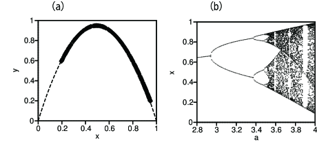
where denotes the control parameter. We demonstrate that a bifurcation diagram can be reproduced using a feedforward neural network. We assume that and are inputs and is the output. The output is considered as the input for the next timestep. That is, feedback from the output layer to the input layer with a time delay of 1 is assumed. The number of neurons in the intermediate layer is , is a random number between -1 and 1, and is a random number between -0.5 and 0.5. The parameter is set to 0.01. The data of for for , 3.4, and 3.9 were used for the Ridge regression. After learning, the outputs for different from 2.8, 3.4, and 3.9 were calculated using the feedforward network.
Figure 1(a) shows the relationship between the input and output for obtained by the feedforward network for the parameter . The dashed line represents for . The input-output relationship of the logistic map was well reproduced by the feedforward network. Figure 1(b) shows the bifurcation diagram obtained by varying . Period-doubling bifurcation and chaos were well reproduced in the feedforward network, although the bifurcation points deviated slightly from those of the logistic map.
Next, we apply the method to mutual synchronization in globally coupled Stuart-Landau equations. As a model of mutual synchronization, we consider the coupled equations of the Stuart-Landau model as follows:
| (5) |
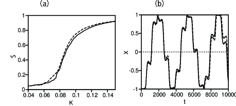
where () is a complex variable, the total number of oscillators is set to , and the natural frequency is selected from a Gaussian random number with an average of 0 and a standard deviation of 0.05. The solid line in Fig. 2(a) shows the order parameter as a function of coupling strength . A phase transition occurs owing to mutual synchronization near .
We consider a three-layer neural network to approximate the nonlinear dynamics of each oscillator. M copies of the three-layer networks are used for the coupled system of oscillators. The input data are , , , , , and , and the outputs are , with . In the learning process, we used 10000 data points of , obtained by direct numerical simulation of the coupled Stuart-Landau equations of three oscillators () with , and -0.03. , 0.1, and 0.15 were selected as the coupling strengths for learning. The number of neurons in the intermediate layer was set to , and . is a random number between -1 and 1, and is a random number between -0.5 and 0.5. , , and are assumed to have the same values for the three networks. Figure 2(b) shows in the coupled Stuart-Landau equation and the feedforward network for and , where the same initial values are used. The nonlinear dynamics of the coupled Stuart-Landau equations is well reproduced by the feedforward network.
The dashed line in Fig. 2(a) shows the order parameter as a function of obtained by the feedforward network of , where and are the same as those obtained by the learning process of , and takes the same Gaussian random number as that in Eq. (5). We input the same values , and into each network. The parameters and are fixed in time, but , , , and change over time. The time-averaged value of the order parameter is plotted as the dashed line in Fig. 2(a). Although the order parameter is slightly different from that of the solid line, the phase transition is reproduced well in the feedforward network.
In summary, we demonstrated that a simple three-layer feedforward network can reproduce the bifurcation diagram of the logistic map and synchronization transition in globally coupled Stuart-Landau equations using data for a few control parameters. We showed that nonlinear mapping close to is approximately reproduced in the feedforward network for the logistic map. That is related to the universal approximation theorem in which an arbitrary function can be approximated in a feedforward network [5]. The advantage of the feedforward network is that the computation time is reduced compared to that of the echo state network because we do not need to repeat the multiple interation of calculations in the intermediate layer.
References
- [1] I. Goodfellow, Y. Bengio, and A. Courville, Deep Learning (MIT Press, 2016).
- [2] H. Jaeger, German National Research Center for Information Technology GMD Technical Report, 148, 13 (2001).
- [3] H. Fan, L.-W. Kong, Y.-C. Lai, and X. Wang, Phys. Rev. Research 3, 023237 (2021).
- [4] F. Rosenblatt, Psychol. Rev. 65, 386 (1958).
- [5] K. Hornik, M. Stinchcombe, and H. White, Neural Network 2, 359 (1989).