Genesis-Metallicity: Universal Non-Parametric Gas-Phase Metallicity Estimation

Abstract

We introduce genesis-metallicity, a gas-phase metallicity measurement python software employing the direct and strong-line methods depending on the available oxygen lines. The non-parametric strong-line estimator is calibrated based on a kernel density estimate in the 4-dimensional space of O2 = [O II]$\lambda\lambda 3727,29$/H$\beta$; O3 = [O III]$\lambda 5007$/H$\beta$; H$\beta$ equivalent width EW(H$\beta$); and gas-phase metallicity $12+\log({\rm O/H)}$. We use a calibration sample of 1551 galaxies at $0<z<10$, with direct-method metallicity measurements compiled from the JWST/NIRSpec and ground-based observations. In particular, we report 145 new NIRSpec direct-method metallicity measurements at $z>1$. We show that the O2, O3, and EW(H$\beta$) measurements are sufficient for a gas-phase metallicity estimate that is more accurate than 0.09 dex. Our calibration is universal, meaning that its accuracy does not depend on the target redshift. Furthermore, the direct-method module employs a non-parametric ${\rm t}_{\rm e}$(O II) electron temperature estimator based on a kernel density estimate in the 5-dimensional space of O2, O3, EW(H$\beta$), ${\rm t}_{\rm e}$(O II), and ${\rm t}_{\rm e}$(O III). This ${\rm t}_{\rm e}$(O II) estimator is calibrated based on 1001 spectra with [O III]$\lambda 4363$ and [O II]$\lambda\lambda 7320,30$ detections, notably reporting 30 new NIRSpec detections of the [O II]$\lambda\lambda 7320,30$ doublet. We make genesis-metallicity and its calibration data publicly available and commit to keeping both up-to-date in light of the incoming data.

1 Introduction

The “direct-method” provides a highly reliable measure of the gas-phase metallicity in galaxies. However, this method relies on an estimate of the electron temperature before the ionic abundances can be derived from the abundance-sensitive emission lines. Unfortunately, the often-faint temperature-sensitive emission lines such as [O III]$\lambda 4363$ and [O II]$\lambda\lambda 7320,30$ remain mostly elusive in large spectroscopic surveys, hindering the application of the direct-method on large samples. This has made the “strong” emission lines such as the [O II]$\lambda\lambda 3727,29$ and [O III]$\lambda 4959,5007$ doublets the most commonly used proxies for the gas-phase metallicities of galaxies with available rest-optical spectroscopy (see, e.g., Savaglio et al., 2005; Erb et al., 2006; Maiolino et al., 2008; Mannucci et al., 2009; Zahid et al., 2011, 2014; Wuyts et al., 2012, 2016; Belli et al., 2013; Henry et al., 2013; Kulas et al., 2013; Cullen et al., 2014; Yabe et al., 2014; Maier et al., 2014; Steidel et al., 2014; Troncoso et al., 2014; Kacprzak et al., 2016, 2015; Sanders et al., 2015, 2021; Hunt et al., 2016; Onodera et al., 2016; Suzuki et al., 2017; Curti et al., 2017, 2024a; Langeroodi et al., 2023; Langeroodi & Hjorth, 2023; Heintz et al., 2023; Nakajima et al., 2023; Chemerynska et al., 2024; Sarkar et al., 2024). This practice is commonly known as the “strong-line” metallicity estimation: several polynomial relations between various strong-line ratios and gas-phase metallicity are calibrated either empirically on samples with direct-method measurements (see, e.g., McGaugh, 1991; Pilyugin et al., 2010; Pilyugin & Grebel, 2016; Curti et al., 2017; Jiang et al., 2019; Nakajima et al., 2022) or against the predictions of photoionization models (see, e.g., McCall et al., 1985; Denicoló et al., 2002; Kewley & Dopita, 2002; Hirschmann et al., 2023).

Despite the success of traditional strong-line metallicity estimators in enabling statistically significant chemical enrichment studies across a wide range of galaxy properties and redshift (see references above), they come with nuanced caveats rooted in their “parametric” nature. Firstly; the 2D projections of the calibration data onto the line ratio vs. metallicity planes risk overlooking the complexities of the higher-order parameter space. Even the 2D projections are often too complex to be fully captured by polynomials. For instance, particularly at low metallicities, large scatter is reported around the best-fit O2–$\log(\rm O/H)$ and O32–$\log(\rm O/H)$ relations. Nakajima et al. (2022) showed that the offsets from these best-fit relations depend on the ionization state of interstellar media (ISM), and can be captured by the equivalent width of H$\beta$, EW(H$\beta$).

Second; the parametric calibrations are prone to “hot” spots which render the estimates in certain metallicity windows highly uncertain. For instance, the best-fit polynomials to the O3–$\log(\rm O/H)$ and R23–$\log(\rm O/H)$ projections are widely used as primary metallicity estimators because these relations exhibit relatively tight scatter. However, both projections are non-monotonic, with a turnover metallicity of $12+\log({\rm O/H)}\sim 8$. This means that i) multiple metallicity solutions exist for each input O3 and R23, which should be sifted based on other projections; ii) the metallicity estimation around the turnover value is highly uncertain due to the flattening of the calibration curve; and iii) observed line ratios higher than the maximum allowed by the calibration curve universally yield the turnover metallicity, failing to capture the intrinsic scatter of the relation.

Third; recent parametric calibrations at high redshifts based on NIRSpec spectroscopy indicate noticeable deviations from the local-universe calibrations (Sanders et al., 2024; Laseter et al., 2024), potentially suggesting a non-universality in the strong-line method. However, as shown by Nakajima et al. (2018) and Nakajima et al. (2022), the 2D-projected relationships between the line ratios and gas-phase metallicity are influenced by the ionization parameter. Therefore, high-redshift deviations from the locally-calibrated parametric strong-line estimators are expected, as the high-redshift galaxies exhibit systematically higher ionization parameters. This is evidenced by their observed extremely high O32, EW(H$\beta$), and EW(H$\alpha$) values (Langeroodi et al., 2023; Langeroodi & Hjorth, 2024; Rinaldi et al., 2023), indicative of high ionization parameters (Kewley & Dopita, 2002; Hirschmann et al., 2023) and bursty star formation histories (Smit et al., 2016; Langeroodi & Hjorth, 2024). Nonetheless, it is essential for any strong-line calibration to capture such dependencies and remain insensitive to these systematics.

Here, we overcome these caveats by developing a “non-parametric” strong-line metallicity estimator. We achieve this by a kernel density estimate (KDE; Silverman, 1986; Scott, 1992) of the probability density function (PDF) in the multi-dimensional space of emission line observables and gas-phase metallicity (Section 4). This PDF is then used to estimate the gas-phase metallicity for any combination of input emission line observables. We calibrate our strong-line estimator on a sample of 1551 galaxies at $0<z<10$ with direct-method metallicity measurements, the largest of such compilations to date (Sections 2 and 3). In particular, we report 145 new direct-method metallicity measurements at $z>1$ based on NIRSpec multi-shutter assembly (MSA; Jakobsen et al., 2022; Ferruit et al., 2022) spectroscopy; this corresponds to a $\sim 6$ fold increase in the sample size of $z>1$ directly-measured metallicities. We show that the O2, O3, and EW(H$\beta$) measurements are sufficient for a gas-phase metallicity estimate that is more accurate than 0.09 dex. Our calibration is universal, meaning that its accuracy does not depend on the target redshift. We make genesis-metallicity and its calibration data available at https://github.com/langeroodi/genesis_metallicity.

2 Data

In this Section, we present an overview of the spectra utilized in our strong-line metallicity calibration. This data consists of 1551 spectra with direct-method metallicity measurements, including 190 galaxies observed with the NIRSpec MSA, 145 of which are reported for the first time in this work and the rest are taken from the literature (Section 2.1); 1213 galaxies observed with ground-based instruments (Section 2.2); and 148 high-metallicity spectra generated by stacking the SDSS spectra (Section 2.3). Figure 1 provides an overview of this sample. The line fluxes are reported in Table 1. We note that the H$\delta$, H$\gamma$, H$\beta$, and H$\alpha$ Balmer lines are used for dust reddening correction of emission lines and EW(H$\beta$). For this purpose, we assumed a Calzetti et al. (2000) dust curve and case-B recombination.

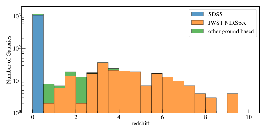
Figure 1: Overview of the calibration sample used in this work. This includes 1551 spectra with direct-method metallicity measurements, including 190 galaxies observed with the NIRSpec MSA (orange), 1213 galaxies observed with ground-based instruments (blue and green), and 148 spectra generated by stacking the SDSS spectra.

2.1 NIRSpec

We searched the JADES DR3 (D’Eugenio et al., 2024) NIRSpec MSA medium-resolution spectra for [O III]$\lambda 4363$ and [O II]$\lambda\lambda 7320,30$ detections. For this purpose, we used pPXF (Cappellari & Emsellem, 2004; Cappellari, 2017, 2022) to measure the emission line fluxes. For the objects covered in multiple JADES observations, we stacked the spectra from repeated gratings to enhance the signal. We adopted the spectroscopic redshifts reported by the JADES team as a starting point, and for each object ran pPXF on the medium-resolution spectra covering its [O III]$\lambda 4363$ and [O II]$\lambda\lambda 7320,30$ emission. We then visually inspected the subsample with either [O III]$\lambda 4363$ or [O II]$\lambda\lambda 7320,30$ flux signal-to-noise ratios (S/N) greater than 3. We confirm 157 galaxies with robust [O III]$\lambda 4363$ detections (${\rm S/N}>3$), 30 of which also exhibit robust [O II]$\lambda\lambda 7320,30$ detection (${\rm S/N}>3$). We also fitted the prism spectra of the [O III]$\lambda 4363$-detected sample to achieve full coverage of the [O II]$\lambda\lambda 3727,29$; H$\gamma$; [O III]$\lambda 4363$; H$\beta$; [O III]$\lambda 4959,5007$; H$\alpha$; and [O II]$\lambda\lambda 7320,30$ lines.

We combined the medium-resolution and prism line flux measurements into a final catalog. We exclusively used the medium resolution measurements for the H$\gamma$, [O III]$\lambda 4363$, and [O II]$\lambda\lambda 7320,30$ lines. This is because in prism spectra H$\gamma$ and [O III]$\lambda 4363$ lines are rarely deblended from one another and [O II]$\lambda\lambda 7320,30$ often appears too faint to be confidently distinguished from the continuum. Since the H$\beta$ to H$\alpha$ flux ratio is the highest-signal Balmer line ratio used to correct for dust attenuation, we prioritized measuring both on the same grating to avoid cross-grating calibration offsets. If multiple gratings provided simultaneous high-significance detections (${\rm S/N}>3$) of both lines, we prioritized medium-resolution gratings as they generally resolve H$\beta$ from [O III]$\lambda 4959,5007$ much more comfortably. The EW(H$\beta$) is calculated using the pPXF best-fit continuum on the same grating where the H$\beta$ flux is read. For the rest of the lines, we used the grating that provides the highest S/N flux measurement. We corrected for cross-grating flux calibration offsets by using the brightest line that is covered in both the medium-resolution and prism gratings. At $z<6$ we avoided the [O III]$\lambda 4959$ and [O III]$\lambda 5007$ lines, since they are often blended in prism spectra. Therefore the flux calibration line is often H$\beta$ or H$\alpha$. When the medium-resolution flux measurement of a line is adopted, its flux is first normalized by the calibration line flux measured in the same grating, and then multiplied by the calibration line flux measured in the prism grating.

We also adopted the NIRSpec MSA line fluxes and EW(H$\beta$) measurements for 33 galaxies from the literature with available direct-method metallicity measurements. This includes 10 galaxies from Nakajima et al. (2023), 14 galaxies from Sanders et al. (2024), and 9 galaxies from Morishita et al. (2024). We note that Laseter et al. (2024) reported 12 galaxies in the JADES DR1 data with direct-method metallicity measurements, which were independently confirmed by the pipeline detailed above.

2.2 Ground-based

Our ground-based spectra consists of 1081 galaxies selected from the archival SDSS spectra (Abazajian et al., 2009); 103 galaxies from the Nakajima et al. (2023) compilation of extremely metal-poor galaxies; 17 galaxies from the Sanders et al. (2020) compilation of $1.5<z<3.5$ direct-method metallicity measurements; and 12 galaxies from the MUSE Ultra Deep Field observations (Revalski et al., 2024). Except for the SDSS galaxies, the line fluxes and EW(H$\beta$) for this sample are adopted from the corresponding papers.

We selected the SDSS galaxies from the MPA-JHU catalog (Tremonti et al., 2004; Brinchmann et al., 2004). We searched for galaxies where all of the [O II]$\lambda\lambda 3727,29$; [O III]$\lambda 4363$; H$\beta$; [O III]$\lambda 5007$; and H$\alpha$ lines are detected with ${\rm S/N}>5$. We sift out the AGNs using the BPT diagram classifications of Brinchmann et al. (2004). We adopted the line fluxes and EW(H$\beta$) as reported in the MPA-JHU catalog. Because the [O II]$\lambda\lambda 7320,30$ flux is not reported in any of the publicly available SDSS catalogs, we used pPXF to measure its flux for the selected galaxies. Out of the 1081 selected galaxies, 876 galaxies exhibit significant [O II]$\lambda\lambda 3727,29$ detections (${\rm S/N}>3$).

2.3 SDSS stacks

Andrews & Martini (2013) and Curti et al. (2017) showed that the individual SDSS spectra can be stacked to enhance the [O III]$\lambda 4363$ signal and enable direct-method metallicity measurements for the less-explored high-metallicity ($8.5<12+\log({\rm O/H)}<9.0$) region of the parameter space. Employing a similar approach, we selected 58207 non-AGN spectra from the MPA-JHU catalog with ${\rm S/N}>5$ [O II]$\lambda\lambda 3727,29$; H$\beta$; [O III]$\lambda 5007$; and H$\alpha$ detections.

We stacked these spectra on a three-dimensional grid of reddening-corrected O2, O3, and EW(H$\beta$). This is in contrast with Curti et al. (2017), where the spectra are stacked on a 2-dimensional grid of reddening-corrected O2 and O3. We chose the 3-dimensional grid because our strong-method calibration relies on O2, O3, and EW(H$\beta$) to estimate the gas-phase metallicity (see Section 4). We binned the O2 axis in 0.1 dex intervals, the O3 axis in 0.1 dex intervals, and the EW(H$\beta$) axis in 1 dex intervals. We stacked the spectra using the stacking algorithm detailed in Langeroodi & Hjorth (2024). We used pPXF to measure the line fluxes and EW(H$\beta$) for the stacks. As reported by Curti et al. (2017), the [Fe II]$\lambda 4360$ line is a common source of systematic offsets in [O III]$\lambda 4363$ flux measurement of very high metallicity galaxies. To avoid such systematics, we add the [Fe II]$\lambda 4360$ line to the list of emission lines fitted by pPXF. We identified 148 stacks with robust [O III]$\lambda 4363$ detections (${\rm S/N}>3$), 108 of which also exhibit significant [O II]$\lambda\lambda 7320,30$ detections (${\rm S/N}>3$).

3 Direct Measurements

We measure the ionic oxygen abundances and gas-phase metallicities (O/H) by modelling the emission lines with a 2-zone H II region (Stasińska, 1982; Garnett, 1992). This corresponds to a bithermal nebula model, where the low-ionization zone containing species such as ${\rm O}^{+}$ and the high-ionization zone containing species such as ${\rm O}^{2+}$ are traced by different temperatures. Assuming an electron density ($n_{\rm e}$), temperature-sensitive line ratios can be used to calculate the electron temperature of each zone. In turn, these temperature measurements allow to derive the ionic abundances of each zone from the abundance-sensitive line fluxes. Where available, we use the [O II]$\lambda\lambda 3727,29$ and [S II]$\lambda\lambda 6717,6731$ lines to estimate the electron densities, while assuming $n_{\rm e}=100\;{\rm cm}^{-3}$ otherwise. The derived temperatures and abundances are only weakly sensitive to the assumed electron density at the density regimes common for galaxies (see, e.g., Curti et al., 2017; Nakajima et al., 2023; Isobe et al., 2023). We describe the electron temperature measurements in Section 3.1 and ionic abundances and gas-phase metallicity measurements in Section 3.2. These measurements are reported in Table 1.

3.1 Electron temperatures

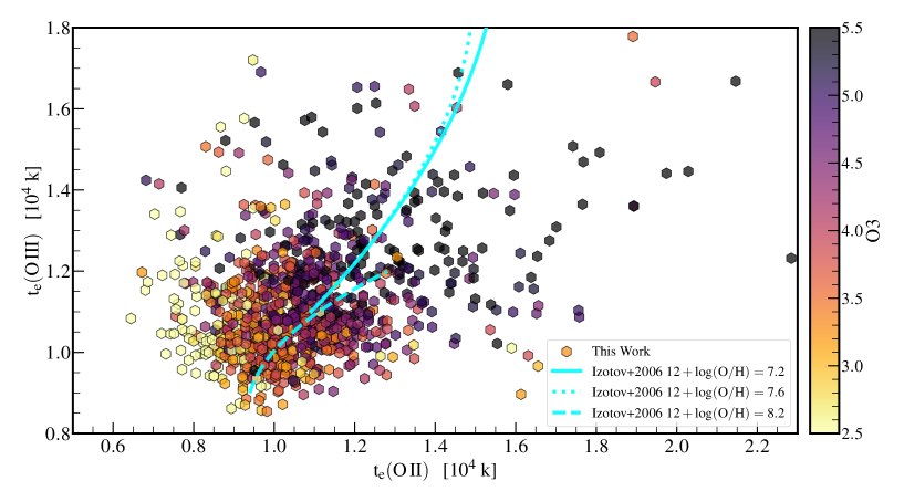
Figure 2: Directly measured ${\rm t}_{\rm e}$(O II) and ${\rm t}_{\rm e}$(O III) for the 1001 spectra where both measurements are available. Each data point is color-coded with its corresponding O3 measurement. The ${\rm t}_{\rm e}$(O II) and ${\rm t}_{\rm e}$(O III) seem to be correlated for average galaxies, with a large scatter that is driven by the O3 value.

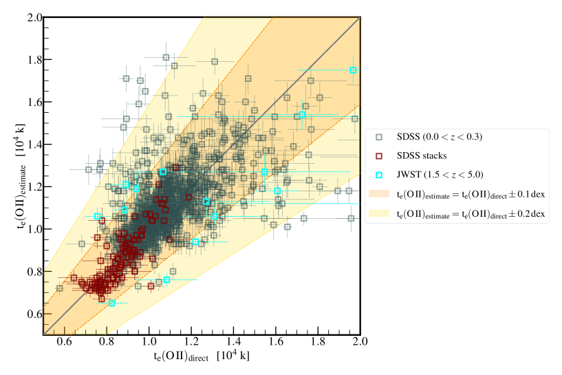
Figure 3: Evaluating the accuracy of the ${\rm t}_{\rm e}$(O II) estimator. Here, we show the ${\rm t}_{\rm e}$(O II) estimates vs. the values measured directly from the [O II]$\lambda\lambda 3727,29$/[O II]$\lambda\lambda 7320,30$ ratios. The ${\rm t}_{\rm e}$(O II) is estimated employing a kernel density estimation of the probability density function in the 5-dimensional space of O2, O3, EW(H$\beta$), ${\rm t}_{\rm e}$(O II), and ${\rm t}_{\rm e}$(O III). The ${\rm t}_{\rm e}$(O II) estimator is more accurate than 0.04 dex, defined as the absolute estimate vs. directly measured ${\rm t}_{\rm e}$(O II) offset that contains $68\%$ of the estimates. The accuracy of the ${\rm t}_{\rm e}$(O II) estimator declines to 0.1 dex at ${\rm t}_{\rm e}$(O II) $>14000$ K, where the parameter space is sparsely sampled by the calibration data (see Figure 2).

We measure the ${\rm O}^{+}$ and ${\rm O}^{2+}$ electron temperatures, denoted as ${\rm t}_{\rm e}$(O II) and ${\rm t}_{\rm e}$(O III), respectively from the [O II]$\lambda\lambda 3727,29$/[O II]$\lambda\lambda 7320,30$ and [O III]$\lambda 4363$/[O III]$\lambda 5007$ flux ratios. We used the getTemDen routine of PyNeb (Luridiana et al., 2012, 2015) for this purpose. This results in ${\rm t}_{\rm e}$(O III) measurements for 1551 spectra, 1001 of which also have ${\rm t}_{\rm e}$(O II) measurements. Figure 2 shows the ${\rm t}_{\rm e}$(O II) and ${\rm t}_{\rm e}$(O III) temperatures for the subample where both measurements are available.

We find that there is a clear empirical trend between ${\rm t}_{\rm e}$(O II), ${\rm t}_{\rm e}$(O III), O2, O3, and EW(H$\beta$). For instance, the ${\rm t}_{\rm e}$(O II)–${\rm t}_{\rm e}$(O III)–O3 trend is shown in Figure 2, where the data points are color-coded with their corresponding O3 measurements. Such relations are expected from the photoionization models (Izotov et al., 2006). In particular, a linear relation between ${\rm t}_{\rm e}$(O II) and ${\rm t}_{\rm e}$(O III) is frequently reported in the literature (Campbell et al., 1986; Garnett, 1992; Izotov et al., 2006; Pilyugin et al., 2006b, a, 2009, 2010; Curti et al., 2017), and often proposed for estimating one temperature from the other when needed (i.e., when the required lines are not covered/detected). Although Figure 2 confirms the proposed trends for average galaxies, it also shows considerable scatter around such relations.

We capture the complex relation between these parameters non-parametrically by employing a kernel density estimate (KDE; Silverman, 1986; Scott, 1992) in the 5-dimensional space of O2, O3, EW(H$\beta$), ${\rm t}_{\rm e}$(O II), and ${\rm t}_{\rm e}$(O III). The multivariate KDE converts the multi-dimensional distribution of data into a non-parametric estimation of the probability density function (PDF). In turn, this PDF can be used to estimate the probability of specific parameter combinations. We estimate the 5-dimensional PDF using the scipy (Virtanen et al., 2020) implementation of the Scott (1992) KDE algorithm with Gaussian kernels. We use the estimated PDF to set up an algorithm, which for each set of input O2, O3, EW(H$\beta$), and ${\rm t}_{\rm e}$(O III) estimates ${\rm t}_{\rm e}$(O II). This particular configuration is chosen because at high redshifts it is often the case where [O II]$\lambda\lambda 3727,29$; [O III]$\lambda 4363$; H$\beta$; and [O III]$\lambda 4959,5007$ are detected, while [O II]$\lambda\lambda 7320,30$ is redshifted out of coverage. As such, it is often the case where measurements of O2, O3, EW(H$\beta$), and ${\rm t}_{\rm e}$(O III) are available, while ${\rm t}_{\rm e}$(O II) cannot be directly measured.

For each set of input O2, O3, EW(H$\beta$), ${\rm t}_{\rm e}$(O III), and their $1\sigma$ uncertainties we make a 4-dimensional grid spanning the $-1\sigma$ to $+1\sigma$ range of each parameter in equally spaced intervals. Assuming that the $-1\sigma$ and $+1\sigma$ uncertainties describe half-Gaussian distributions, we assign a weight to each grid point in this 4-dimensional space. At each grid point, we calculate the probability along the ${\rm t}_{\rm e}$(O II) axis in 10 K intervals. The resulting 1-dimensional PDFs are multiplied by the weights of the corresponding grid points and then combined to make a 1-dimensional ${\rm t}_{\rm e}$(O II) PDF. This PDF is used to estimate the best-fit ${\rm t}_{\rm e}$(O II) and its uncertainty as the highest-probability point and the $1\sigma$ region.

We evaluate the accuracy of our ${\rm t}_{\rm e}$(O II) estimator through a leave-one-out cross-validation approach. In each iteration we take out one data point from the calibration sample, use the KDE on the remaining data points to estimate the 5-dimensional PDF, and apply the resulting ${\rm t}_{\rm e}$(O II) estimator on the O2, O3, EW(H$\beta$), and ${\rm t}_{\rm e}$(O III) of the removed data point to estimate its ${\rm t}_{\rm e}$(O II). Figure 3 shows the estimated ${\rm t}_{\rm e}$(O II) vs. the directly measured values. The ${\rm t}_{\rm e}$(O II) estimator is more accurate than 0.04 dex, defined as the absolute estimate vs. directly measured ${\rm t}_{\rm e}$(O II) offset that contains $68\%$ of the estimates. As shown in Figure 3, the accuracy of our ${\rm t}_{\rm e}$(O II) estimator declines to 0.1 dex at ${\rm t}_{\rm e}$(O II) $>14000$ K, where the parameter space is sparsely sampled (see Figure 2).

3.2 Metallicities

We calculate the ${\rm O}^{2+}$ ionic abundances from the [O III]$\lambda 4959,5007$/H$\beta$ line ratios, employing the getIonAbundance routine of PyNeb and assuming the ${\rm t}_{\rm e}$(O III) electron temperatures calculated in Section 3.1. Similarly, the ${\rm O}^{+}$ ionic abundances are calculated from the [O II]$\lambda\lambda 3727,29$/H$\beta$ line ratios, assuming the ${\rm t}_{\rm e}$(O II) electron temperatures calculated in Section 3.1. Whenever there is no ${\rm t}_{\rm e}$(O II) measurement available, we used the ${\rm t}_{\rm e}$(O II) estimator calibrated in Section 3.1 to estimate the ${\rm t}_{\rm e}$(O II) based on the measured O2, O3, EW(H$\beta$), and ${\rm t}_{\rm e}$(O III). We assume that the ${\rm O}^{+}$ and ${\rm O}^{2+}$ are the most abundant oxygen ions, and derive the oxygen abundances (gas-phase metallicity) as the sum of ${\rm O}^{+}$ and ${\rm O}^{2+}$ ionic abundances.

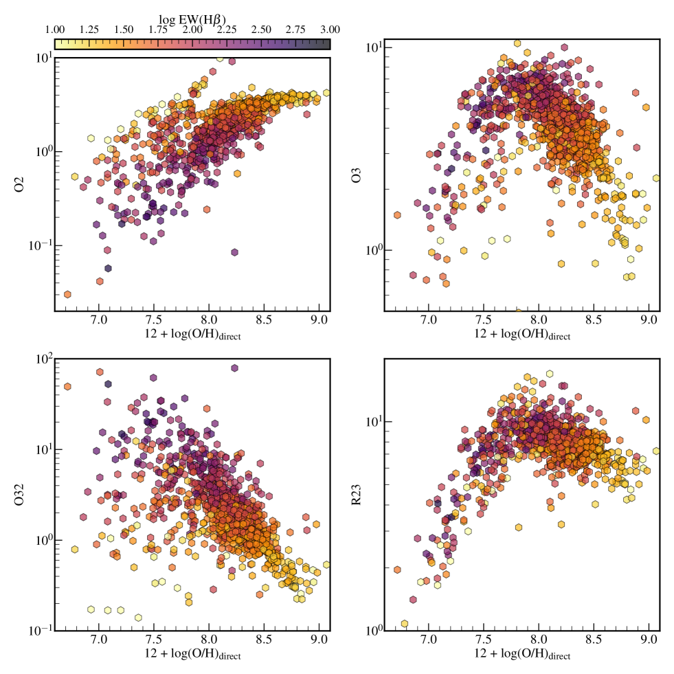
Figure 4: Classic projections of the calibration data onto the 2D planes of O2-$\log(\rm O/H)$, O3-$\log(\rm O/H)$, O32-$\log(\rm O/H)$, and R23-$\log(\rm O/H)$. Each data point is color-coded with its EW(H$\beta$) value. These projections are often used for parametric strong-line metallicity calibrations. We note that these projections are provided here for completeness, and our metallicity estimator is instead calibrated non-parametrically in the 4-dimensional space of O2, O3, EW(H$\beta$), and gas-phase metallicity (see Section 4) for details.

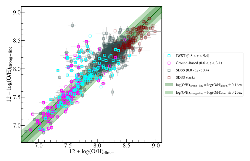
Figure 5: Evaluating the accuracy of the strong-line metallicity estimator. Here, we show the strong-line vs. direct-method metallicities for the calibration sample. This plot is generated through a leave-one-out cross-validation approach. In brief, in each iteration we exclude one data point from the calibration sample, calibrate the metallicity estimator on the remaining sample, and use this estimator to estimate the metallicity of the excluded point based on its O2, O3, and EW(H$\beta$). The strong-line metallicity estimator is more accurate than 0.09 dex, defined as the absolute strong-line vs. direct metallicity offset containing $68\%$ of the estimates. Our calibration is universal, meaning that its accuracy does not depend on the target redshift.

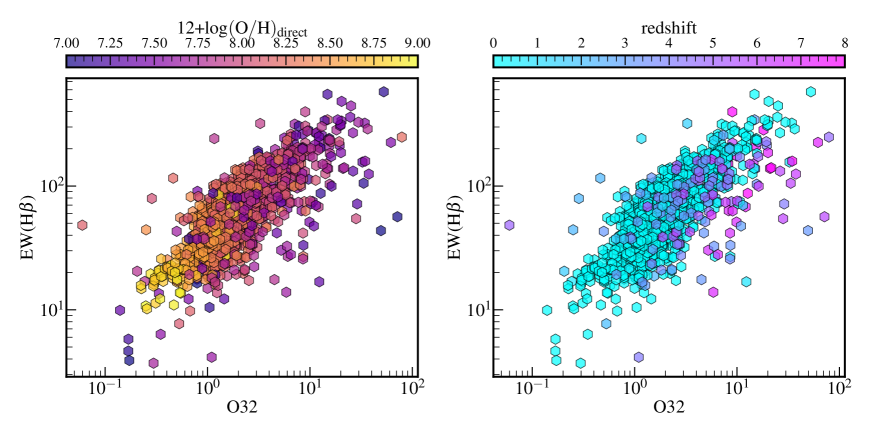
Figure 6: Tight correlation between the O32 line ratio and EW(H$\beta$). Since the O32 is an ionization parameter estimator, this correlation suggests that EW(H$\beta$) can also be used to trace the ionization parameter. In the left panel the data points are color-coded with their corresponding directly-measured metallicities. In the right panel the data points are color-coded with their corresponding redshifts.

4 Strong-line calibration

We use the distribution of the calibration data in the 4-dimensional space of O2, O3, EW(H$\beta$), and gas-phase metallicity for a non-parametric calibration of a strong-line metallicity estimator. Figure 4 shows 4 classic projections of the data, frequently used for the parametric calibration of the strong-line metallicity estimators. We adapt a method similar to that described in Section 3.1 for the non-parametric calibration. In brief, we use a kernel density estimate (KDE) in the 4-dimensional space of O2, O3, EW(H$\beta$), and gas-phase metallicity to estimate the probability density function (PDF) non-parametrically based on the distribution of the calibration data. This PDF is then used to estimate the gas-phase metallicity for any combination of input O2, O3, and EW(H$\beta$). The marginalization procedure is described in detail in Section 3.1. In this calibration, we only include the subsample with direct-method metallicity uncertainties lower than 0.2 dex.

We evaluate the accuracy of our strong-line metallicity estimator with a leave-one-out cross-validation approach, similar to that described in Section 3.1. In each iteration, we exclude one data point from the calibration sample, calibrate the metallicity estimator on the remaining data, and use this estimator to estimate the metallicity of the excluded point based on its O2, O3, and EW(H$\beta$) measurements. Figure 5 shows the strong-line gas-phase metallicity estimates vs. those measured by the direct method. Our metallicity estimations are more accurate than 0.09 dex, defined as the absolute strong-line vs. direct metallicity offset which contains $68\%$ of the estimates.

The accuracy of our strong-line metallicity estimator does not vary noticeably with redshift. We achieve a 0.09 dex accuracy at $z<0.5$, 0.12 dex accuracy at $z>0.5$, and a 0.13 dex accuracy at $z>1.0$. We further confirm this by adding the source redshift as an extra dimension to the kernel density estimate and re-calibrating the strong-line metallicity estimator. Repeating the same leave-one-out cross-validation test as above, we achieve identical accuracies at $z<0.5$, $z>0.5$, and $z>1.0$. This highlights that adding the redshift provides no additional information for estimating the gas-phase metallicities beyond what is already captured by O2, O3, and EW(H$\beta$).

As shown in Figure 6, EW(H$\beta$) and O32 are tightly correlated. Since O32 is widely accepted as an ionization parameter estimator (see, e.g., Kewley & Dopita, 2002; Hirschmann et al., 2023), this correlation suggests that EW(H$\beta$) closely traces the ionization parameter as well. Photoionization models imply that the relationship between the strong-line ratios and gas-phase metallicity is sensitive to the ionization parameter (Nakajima et al., 2018, 2022). As such, including an ionization parameter estimator such as O32 or EW(H$\beta$) in the strong-line metallicity calibration is expected to increase its accuracy. Indeed, Nakajima et al. (2022) showed that the parametric strong-line metallicity calibration can be improved, particularly at the low-metallicity end, by splitting calibration into three ionization branches as traced by the observed EW(H$\beta$).

The tight correlation between the EW(H$\beta$) and O32 (see Figure 6) might suggest that O2 and O3 should be sufficient to calibrate an optimal strong-line metallicity estimator; i.e., suggesting that including the EW(H$\beta$) information is unnecessary. This is because EW(H$\beta$) is accurately predicted from its tight correlation with O32, and the O32 information is already captured by including the O2 and O3. We test this by removing the EW(H$\beta$) axis from our strong-line metallicity calibration, which slightly yet noticeably decreases the accuracy of our metallicity estimator to 0.17 dex. Hence, EW(H$\beta$) is providing additional information beyond what is captured by O2 and O3. This seems intuitive from Figure 6, where the offset from the average EW(H$\beta$)-O3 relation seems to correlate with both the gas-phase metallicity and redshift, as indicated by the color-coding in the left and right panels, respectively. Similarly, we find that including the EW(H$\beta$) information slightly improves the accuracy of our ${\rm t}_{\rm e}$(O II) estimator (Section 3.1).

5 Conclusion

We present genesis-metallicity, a non-parametric electron temperature and gas-phase metallicity estimator. This code is calibrated on a sample of 1551 [O III]$\lambda 4363$ detections at $0<z<10$, compiled from the JWST/NIRSpec and ground-based observations. In particular, we report 145 new NIRSpec direct-method metallicity measurements at $z>1$; this corresponds to a $\sim 6$ fold increase in the sample size of $z>1$ directly-measured metallicities.

The electron temperature estimator is calibrated based on a kernel density estimate of the probability density function in the 5-dimensional space of O2, O3, EW(H$\beta$), ${\rm t}_{\rm e}$(O II), and ${\rm t}_{\rm e}$(O III). We achieve a 0.04 dex accuracy in our ${\rm t}_{\rm e}$(O II) estimates. The strong-line metallicity estimator is calibrated in the 4-dimensional space of O2, O3, EW(H$\beta$), and gas-phase metallicity. We achieve a 0.09 dex accuracy in our strong-line gas-phase metallicity estimates. Our calibration is universal, meaning that its accuracy does not depend on the target redshift.

Improved sampling of the sparsely populated regions of the emission line observables parameter space can further enhance the accuracy of our calibration. Therefore, we commit to keeping genesis-metallicity and its calibration data up-to-date in light of the upcoming data. The most recent version of genesis-metallicity and its calibration data can be found at https://github.com/langeroodi/genesis_metallicity.

Table 1: Inferred Properties for the Galaxies in the Calibration Sample. Only a small subsample of the calibration data and inferred properties are presented here. The full table containing 1551 galaxies, along with their sky coordinates, observed and reddening-corrected line fluxes, and MSA IDs (for the JWST sources) are available at https://github.com/langeroodi/genesis_metallicity

ID	Redshift	$A_{\rm V}$	${\rm t}_{\rm e}$(O II)	${\rm t}_{\rm e}$(O III)	Metallicity
		mag	[$10^{4}$ K]	[$10^{4}$ K]	$12+\log({\rm O/H)}$
JADES-DR3-3	3.91	3.14	$1.3\pm 0.1$	$2.4\pm 0.1$	$7.61\pm 0.03$
JADES-DR3-38	4.41	3.16	$1.3\pm 0.1$	$2.4\pm 0.2$	$7.96\pm 0.05$
JADES-DR3-47	4.70	0.00	$1.5\pm 0.1$	$1.3\pm 0.1$	$8.11\pm 0.12$
JADES-DR3-50	6.76	3.68	$1.4\pm 0.1$	$2.2\pm 0.2$	$7.47\pm 0.06$
JADES-DR3-51	5.42	3.95	$1.5\pm 0.0$	$2.1\pm 0.2$	$7.66\pm 0.04$
JADES-DR3-56	6.31	0.69	$1.5\pm 0.0$	$1.9\pm 0.1$	$7.41\pm 0.05$
JADES-DR3-67	3.87	1.23	$1.9\pm 0.6$	$1.4\pm 0.1$	$8.04\pm 0.07$
JADES-DR3-76	3.80	1.71	$1.5\pm 0.0$	$1.9\pm 0.3$	$7.74\pm 0.13$
JADES-DR3-84	3.34	0.37	$1.7\pm 0.3$	$2.2\pm 0.2$	$7.49\pm 0.07$
JADES-DR3-85	7.09	3.04	$1.5\pm 0.0$	$2.0\pm 0.3$	$7.71\pm 0.09$
JADES-DR3-104	3.33	0.60	$1.5\pm 0.0$	$1.8\pm 0.1$	$7.73\pm 0.04$
JADES-DR3-138	5.66	1.49	$1.3\pm 0.0$	$2.4\pm 0.0$	$7.83\pm 0.05$
JADES-DR3-164	3.36	0.57	$1.5\pm 0.1$	$2.1\pm 0.3$	$7.90\pm 0.08$
JADES-DR3-170	4.70	0.99	$1.3\pm 0.0$	$2.4\pm 0.0$	$7.62\pm 0.02$
JADES-DR3-173	3.66	1.66	$2.9\pm 0.1$	$2.4\pm 0.1$	$7.33\pm 0.02$
JADES-DR3-184	4.53	0.00	$1.6\pm 0.1$	$1.2\pm 0.1$	$8.16\pm 0.09$
JADES-DR3-249	5.99	0.00	$1.3\pm 0.0$	$2.4\pm 0.1$	$7.60\pm 0.04$
JADES-DR3-254	3.24	1.60	$1.8\pm 0.3$	$1.4\pm 0.1$	$7.95\pm 0.06$
JADES-DR3-295	2.98	2.90	$1.3\pm 0.1$	$2.4\pm 0.2$	$7.84\pm 0.04$
JADES-DR3-307	7.00	1.28	$1.4\pm 0.1$	$2.4\pm 0.2$	$7.56\pm 0.04$
JADES-DR3-333	6.82	0.00	$1.5\pm 0.1$	$2.1\pm 0.3$	$7.61\pm 0.09$
JADES-DR3-350	2.96	1.89	$1.5\pm 0.0$	$2.4\pm 0.0$	$7.36\pm 0.09$
JADES-DR3-363	4.41	0.00	$1.9\pm 0.1$	$1.3\pm 0.0$	$8.05\pm 0.03$
JADES-DR3-366	4.06	1.05	$1.4\pm 0.1$	$1.6\pm 0.3$	$7.90\pm 0.12$
JADES-DR3-380	7.09	0.76	$1.5\pm 0.0$	$2.1\pm 0.1$	$7.50\pm 0.04$
JADES-DR3-401	3.87	1.79	$1.0\pm 0.1$	$1.0\pm 0.1$	$8.55\pm 0.13$
JADES-DR3-405	4.38	0.00	$3.0\pm 0.0$	$1.1\pm 0.1$	$8.36\pm 0.11$
JADES-DR3-415	3.32	0.00	$1.5\pm 0.0$	$2.4\pm 0.0$	$7.25\pm 0.25$
JADES-DR3-419	6.67	0.00	$1.5\pm 0.1$	$2.1\pm 0.3$	$7.60\pm 0.08$
JADES-DR3-420	6.81	0.00	$1.7\pm 0.1$	$1.1\pm 0.1$	$8.29\pm 0.11$

References

- Abazajian et al. (2009) Abazajian, K. N., Adelman-McCarthy, J. K., Agüeros, M. A., et al. 2009, ApJS, 182, 543, doi: 10.1088/0067-0049/182/2/543
- Andrews & Martini (2013) Andrews, B. H., & Martini, P. 2013, ApJ, 765, 140, doi: 10.1088/0004-637X/765/2/140
- Belli et al. (2013) Belli, S., Jones, T., Ellis, R. S., & Richard, J. 2013, ApJ, 772, 141, doi: 10.1088/0004-637X/772/2/141
- Brinchmann et al. (2004) Brinchmann, J., Charlot, S., White, S. D. M., et al. 2004, MNRAS, 351, 1151, doi: 10.1111/j.1365-2966.2004.07881.x
- Calzetti et al. (2000) Calzetti, D., Armus, L., Bohlin, R. C., et al. 2000, ApJ, 533, 682, doi: 10.1086/308692
- Campbell et al. (1986) Campbell, A., Terlevich, R., & Melnick, J. 1986, MNRAS, 223, 811, doi: 10.1093/mnras/223.4.811
- Cappellari (2017) Cappellari, M. 2017, MNRAS, 466, 798, doi: 10.1093/mnras/stw3020
- Cappellari (2022) —. 2022, MNRAS submitted, doi: 10.48550/arXiv.2208.14974
- Cappellari & Emsellem (2004) Cappellari, M., & Emsellem, E. 2004, PASP, 116, 138, doi: 10.1086/381875
- Chemerynska et al. (2024) Chemerynska, I., Atek, H., Dayal, P., et al. 2024, arXiv e-prints, arXiv:2407.17110, doi: 10.48550/arXiv.2407.17110
- Cullen et al. (2014) Cullen, F., Cirasuolo, M., McLure, R. J., Dunlop, J. S., & Bowler, R. A. A. 2014, MNRAS, 440, 2300, doi: 10.1093/mnras/stu443
- Curti et al. (2017) Curti, M., Cresci, G., Mannucci, F., et al. 2017, MNRAS, 465, 1384, doi: 10.1093/mnras/stw2766
- Curti et al. (2024a) Curti, M., Maiolino, R., Curtis-Lake, E., et al. 2024a, A&A, 684, A75, doi: 10.1051/0004-6361/202346698
- Curti et al. (2024b) Curti, M., Witstok, J., Jakobsen, P., et al. 2024b, arXiv e-prints, arXiv:2407.02575, doi: 10.48550/arXiv.2407.02575
- Denicoló et al. (2002) Denicoló, G., Terlevich, R., & Terlevich, E. 2002, MNRAS, 330, 69, doi: 10.1046/j.1365-8711.2002.05041.x
- D’Eugenio et al. (2024) D’Eugenio, F., Cameron, A. J., Scholtz, J., et al. 2024, arXiv e-prints, arXiv:2404.06531, doi: 10.48550/arXiv.2404.06531
- Erb et al. (2006) Erb, D. K., Shapley, A. E., Pettini, M., et al. 2006, ApJ, 644, 813, doi: 10.1086/503623
- Ferruit et al. (2022) Ferruit, P., Jakobsen, P., Giardino, G., et al. 2022, A&A, 661, A81, doi: 10.1051/0004-6361/202142673
- Garnett (1992) Garnett, D. R. 1992, AJ, 103, 1330, doi: 10.1086/116146
- Heintz et al. (2023) Heintz, K. E., Brammer, G. B., Giménez-Arteaga, C., et al. 2023, Nature Astronomy, 7, 1517, doi: 10.1038/s41550-023-02078-7
- Henry et al. (2013) Henry, A., Scarlata, C., Domínguez, A., et al. 2013, ApJ, 776, L27, doi: 10.1088/2041-8205/776/2/L27
- Hirschmann et al. (2023) Hirschmann, M., Charlot, S., & Somerville, R. S. 2023, MNRAS, 526, 3504, doi: 10.1093/mnras/stad2745
- Hunt et al. (2016) Hunt, L., Dayal, P., Magrini, L., & Ferrara, A. 2016, MNRAS, 463, 2002, doi: 10.1093/mnras/stw1993
- Isobe et al. (2023) Isobe, Y., Ouchi, M., Nakajima, K., et al. 2023, ApJ, 956, 139, doi: 10.3847/1538-4357/acf376
- Izotov et al. (2006) Izotov, Y. I., Stasińska, G., Meynet, G., Guseva, N. G., & Thuan, T. X. 2006, A&A, 448, 955, doi: 10.1051/0004-6361:20053763
- Jakobsen et al. (2022) Jakobsen, P., Ferruit, P., Alves de Oliveira, C., et al. 2022, A&A, 661, A80, doi: 10.1051/0004-6361/202142663
- Jiang et al. (2019) Jiang, T., Malhotra, S., Rhoads, J. E., & Yang, H. 2019, ApJ, 872, 145, doi: 10.3847/1538-4357/aaee8a
- Kacprzak et al. (2015) Kacprzak, G. G., Yuan, T., Nanayakkara, T., et al. 2015, ApJ, 802, L26, doi: 10.1088/2041-8205/802/2/L26
- Kacprzak et al. (2016) Kacprzak, G. G., van de Voort, F., Glazebrook, K., et al. 2016, ApJ, 826, L11, doi: 10.3847/2041-8205/826/1/L11
- Kewley & Dopita (2002) Kewley, L. J., & Dopita, M. A. 2002, ApJS, 142, 35, doi: 10.1086/341326
- Kulas et al. (2013) Kulas, K. R., McLean, I. S., Shapley, A. E., et al. 2013, ApJ, 774, 130, doi: 10.1088/0004-637X/774/2/130
- Langeroodi & Hjorth (2023) Langeroodi, D., & Hjorth, J. 2023, arXiv e-prints, arXiv:2307.06336, doi: 10.48550/arXiv.2307.06336
- Langeroodi & Hjorth (2024) —. 2024, arXiv e-prints, arXiv:2404.13045, doi: 10.48550/arXiv.2404.13045
- Langeroodi et al. (2023) Langeroodi, D., Hjorth, J., Chen, W., et al. 2023, ApJ, 957, 39, doi: 10.3847/1538-4357/acdbc1
- Laseter et al. (2024) Laseter, I. H., Maseda, M. V., Curti, M., et al. 2024, A&A, 681, A70, doi: 10.1051/0004-6361/202347133
- Luridiana et al. (2012) Luridiana, V., Morisset, C., & Shaw, R. A. 2012, in IAU Symposium, Vol. 283, Planetary Nebulae: An Eye to the Future, 422–423, doi: 10.1017/S1743921312011738
- Luridiana et al. (2015) Luridiana, V., Morisset, C., & Shaw, R. A. 2015, A&A, 573, A42, doi: 10.1051/0004-6361/201323152
- Maier et al. (2014) Maier, C., Lilly, S. J., Ziegler, B. L., et al. 2014, ApJ, 792, 3, doi: 10.1088/0004-637X/792/1/3
- Maiolino et al. (2008) Maiolino, R., Nagao, T., Grazian, A., et al. 2008, A&A, 488, 463, doi: 10.1051/0004-6361:200809678
- Mannucci et al. (2009) Mannucci, F., Cresci, G., Maiolino, R., et al. 2009, MNRAS, 398, 1915, doi: 10.1111/j.1365-2966.2009.15185.x
- McCall et al. (1985) McCall, M. L., Rybski, P. M., & Shields, G. A. 1985, ApJS, 57, 1, doi: 10.1086/190994
- McGaugh (1991) McGaugh, S. S. 1991, ApJ, 380, 140, doi: 10.1086/170569
- Morishita et al. (2024) Morishita, T., Stiavelli, M., Grillo, C., et al. 2024, arXiv e-prints, arXiv:2402.14084, doi: 10.48550/arXiv.2402.14084
- Nakajima et al. (2023) Nakajima, K., Ouchi, M., Isobe, Y., et al. 2023, ApJS, 269, 33, doi: 10.3847/1538-4365/acd556
- Nakajima et al. (2018) Nakajima, K., Schaerer, D., Le Fèvre, O., et al. 2018, A&A, 612, A94, doi: 10.1051/0004-6361/201731935
- Nakajima et al. (2022) Nakajima, K., Ouchi, M., Xu, Y., et al. 2022, ApJS, 262, 3, doi: 10.3847/1538-4365/ac7710
- Onodera et al. (2016) Onodera, M., Carollo, C. M., Lilly, S., et al. 2016, ApJ, 822, 42, doi: 10.3847/0004-637X/822/1/42
- Pilyugin & Grebel (2016) Pilyugin, L. S., & Grebel, E. K. 2016, MNRAS, 457, 3678, doi: 10.1093/mnras/stw238
- Pilyugin et al. (2009) Pilyugin, L. S., Mattsson, L., Vílchez, J. M., & Cedrés, B. 2009, MNRAS, 398, 485, doi: 10.1111/j.1365-2966.2009.15182.x
- Pilyugin et al. (2006a) Pilyugin, L. S., Thuan, T. X., & Vílchez, J. M. 2006a, MNRAS, 367, 1139, doi: 10.1111/j.1365-2966.2006.10033.x
- Pilyugin et al. (2006b) Pilyugin, L. S., Vílchez, J. M., & Thuan, T. X. 2006b, MNRAS, 370, 1928, doi: 10.1111/j.1365-2966.2006.10618.x
- Pilyugin et al. (2010) —. 2010, ApJ, 720, 1738, doi: 10.1088/0004-637X/720/2/1738
- Revalski et al. (2024) Revalski, M., Rafelski, M., Henry, A., et al. 2024, ApJ, 966, 228, doi: 10.3847/1538-4357/ad382c
- Rinaldi et al. (2023) Rinaldi, P., Caputi, K. I., Costantin, L., et al. 2023, ApJ, 952, 143, doi: 10.3847/1538-4357/acdc27
- Sanders et al. (2024) Sanders, R. L., Shapley, A. E., Topping, M. W., Reddy, N. A., & Brammer, G. B. 2024, ApJ, 962, 24, doi: 10.3847/1538-4357/ad15fc
- Sanders et al. (2015) Sanders, R. L., Shapley, A. E., Kriek, M., et al. 2015, ApJ, 799, 138, doi: 10.1088/0004-637X/799/2/138
- Sanders et al. (2020) Sanders, R. L., Shapley, A. E., Reddy, N. A., et al. 2020, MNRAS, 491, 1427, doi: 10.1093/mnras/stz3032
- Sanders et al. (2021) Sanders, R. L., Shapley, A. E., Jones, T., et al. 2021, ApJ, 914, 19, doi: 10.3847/1538-4357/abf4c1
- Sarkar et al. (2024) Sarkar, A., Chakraborty, P., Vogelsberger, M., et al. 2024, arXiv e-prints, arXiv:2408.07974, doi: 10.48550/arXiv.2408.07974
- Savaglio et al. (2005) Savaglio, S., Glazebrook, K., Le Borgne, D., et al. 2005, ApJ, 635, 260, doi: 10.1086/497331
- Schaerer et al. (2024) Schaerer, D., Marques-Chaves, R., Xiao, M., & Korber, D. 2024, A&A, 687, L11, doi: 10.1051/0004-6361/202450721
- Scott (1992) Scott, D. W. 1992, Multivariate Density Estimation
- Silverman (1986) Silverman, B. W. 1986, Density estimation for statistics and data analysis
- Smit et al. (2016) Smit, R., Bouwens, R. J., Labbé, I., et al. 2016, ApJ, 833, 254, doi: 10.3847/1538-4357/833/2/254
- Stasińska (1982) Stasińska, G. 1982, A&AS, 48, 299
- Steidel et al. (2014) Steidel, C. C., Rudie, G. C., Strom, A. L., et al. 2014, ApJ, 795, 165, doi: 10.1088/0004-637X/795/2/165
- Suzuki et al. (2017) Suzuki, T. L., Kodama, T., Onodera, M., et al. 2017, ApJ, 849, 39, doi: 10.3847/1538-4357/aa8df3
- Tremonti et al. (2004) Tremonti, C. A., Heckman, T. M., Kauffmann, G., et al. 2004, ApJ, 613, 898, doi: 10.1086/423264
- Troncoso et al. (2014) Troncoso, P., Maiolino, R., Sommariva, V., et al. 2014, A&A, 563, A58, doi: 10.1051/0004-6361/201322099
- Virtanen et al. (2020) Virtanen, P., Gommers, R., Oliphant, T. E., et al. 2020, Nature Methods, 17, 261, doi: 10.1038/s41592-019-0686-2
- Williams et al. (2023) Williams, H., Kelly, P. L., Chen, W., et al. 2023, Science, 380, 416, doi: 10.1126/science.adf5307
- Wuyts et al. (2012) Wuyts, E., Rigby, J. R., Sharon, K., & Gladders, M. D. 2012, ApJ, 755, 73, doi: 10.1088/0004-637X/755/1/73
- Wuyts et al. (2016) Wuyts, E., Wisnioski, E., Fossati, M., et al. 2016, ApJ, 827, 74, doi: 10.3847/0004-637X/827/1/74
- Yabe et al. (2014) Yabe, K., Ohta, K., Iwamuro, F., et al. 2014, MNRAS, 437, 3647, doi: 10.1093/mnras/stt2185
- Zahid et al. (2011) Zahid, H. J., Kewley, L. J., & Bresolin, F. 2011, ApJ, 730, 137, doi: 10.1088/0004-637X/730/2/137
- Zahid et al. (2014) Zahid, H. J., Kashino, D., Silverman, J. D., et al. 2014, ApJ, 792, 75, doi: 10.1088/0004-637X/792/1/75