Introducing Perturb-ability Score (PS) to Enhance Robustness Against Evasion Adversarial Attacks on ML-NIDS
Authors’ draft for soliciting feedback

Abstract

This paper proposes a novel Perturb-ability Score (PS) that can be used to identify Network Intrusion Detection Systems (NIDS) features that can be easily manipulated by attackers in the problem-space. We demonstrate that using PS to select only non-perturb-able features for ML-based NIDS maintains detection performance while enhancing robustness against adversarial attacks.

L1/.style=fill=white,, L2/.style=fill=red,edge=red,line width=2pt, L3/.style=fill=yellow,edge=yellow,line width=2pt, L4/.style=fill=green,edge=green,line width=2pt,

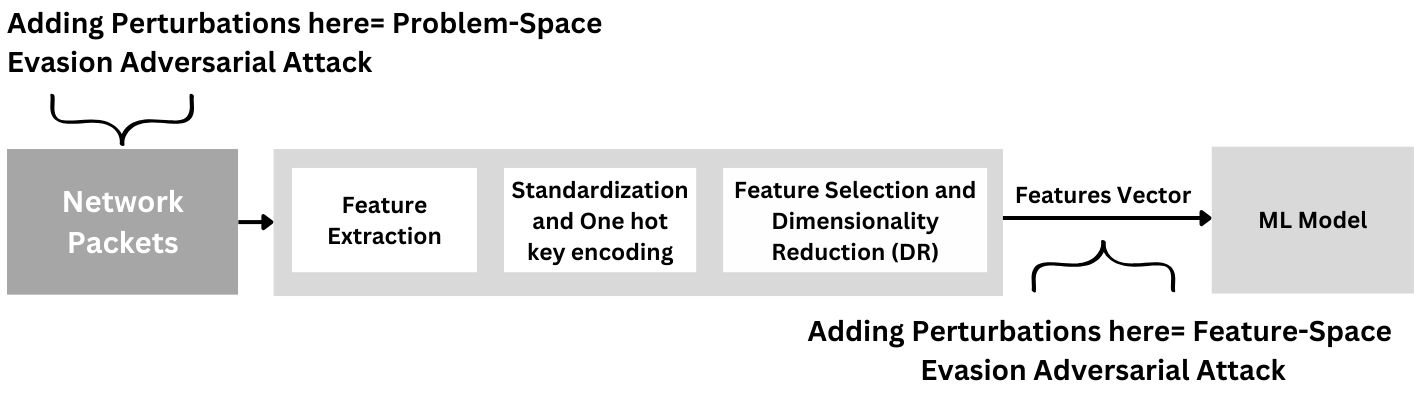
Figure 1: Evasion Adversarial Attacks in Feature-Space vs Problem-Space Against NIDS

1 Introduction

Machine Learning (ML) is widely employed in Network Intrusion Detection Systems (NIDS) due to its high accuracy in classifying large volumes of data [1]. NIDS play a critical role in protecting computer networks by identifying malicious traffic. However, ML-based NIDS models can be the target of evasion adversarial attacks [2]. These attacks aim to deceive the ML model during decision-making by modifying or adding carefully crafted perturbations to the input data, often based on the gradient of the target ML model.

Evasion Adversarial Attacks in Feature-Space vs Problem-Space: Ibitoye et al. [2] introduced the concept of ”space” in the taxonomy of adversarial attacks for network security, distinguishing between feature-space (manipulating feature vectors) and problem-space attacks (modifying actual data), see Figure 1.

Feature-space attacks may not be practical against NIDS due to challenges an attacker would face in feature vector access and challenges with feature correlations and network constraints [6]. On the other hand, problem-space attacks are more practical than feature-space as the modifications happen to the network packets (feasible for an external attacker). They typically start with feature-space perturbations, then translate to real-world packet modifications (Inverse Feature-Mapping [5]). Despite being considered more practical than feature-space attacks, these attacks also face several practicality issues [6], such as: challenges in maintaining malicious intent and network functionality while altering packets; keeping up-to-date knowledge of the model, its features, and extraction techniques; or predicting correct common features. Problem-space attacks must also address NIDS features constraints.

Perturb-ability of Features in Problem-Space Against NIDS: Problem-space evasion attacks on NIDS involve modifying network packets with the aim of resulting in manipulations to some features within the feature vector. Perturbing certain NIDS features within the problem-space, without affecting network functionality, might be achievable, for instance, adding padding to payloads or introducing delays between packets perturbs length and interarrival time features (Figure 2a). However, problem-space constraints significantly limit the perturb-ability of many other NIDS features. For example, modifying the destination IP or port number disrupts network functionality (Figure 2b), and some features, like backward and inter-flow/-connection features, are inaccessible for modification. N.B., by non-perturb-able features, we mean features that cannot be perturbed in the problem-space while complying with network constraints. Perturb-able features are the opposite.

2 Perturb-ability Score (PS)

We introduce the Perturb-ability Score (PS) to quantify each feature’s perturb-ability. We also discuss how PS classifies NIDS features and enables a defense against practical problem-space evasion attacks.

(a) Examples of Perturb-able Features
in Problem-Space Against NIDS

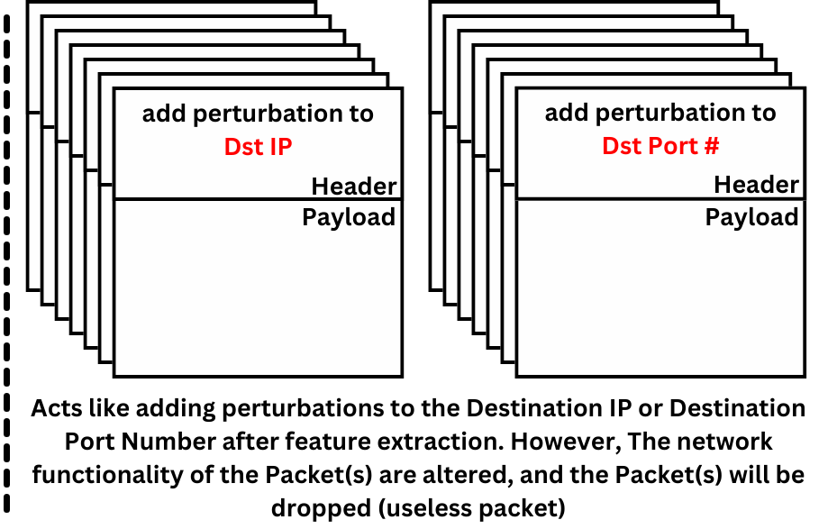
(b) Examples of Non-Perturb-able Features
in Problem-Space Against NIDS

Figure 2: Examples of Perturb-able vs Non-Perturb-able Features in Network Traffic

2.1 Evaluating PS

The goal of PS is to obtain a Perturb-ability score for each feature ($f_{i}$) in a dataset $D$, where $i$ is the ID of the feature from 1 to $n$, and $n$ is the number of features in $D$. PS should range from 0 (features extremely hard to perturb in problem-space while maintaining the networks constraints) to 1 (features can be perturbed in problem-space while maintaining the networks constraints). The $PS_{Total}[f_{i}]$ is the geometric average of the following five fields:

2.1.1 PS₁[$f_{i}$]: Strict Header Features/ Affects Network or Malicious Functionality:

This PS field focuses on strict Header features and network/malicious functionality of network flows after adding perturbations in the problem-space. PS₁[$f_{i}$] will be 0 if any of the following conditions are true (which will make PS_Total[$f_{i}$] equals 0);

C1: the feature $f_{i}$ is a strict header feature (IP addresses in TCP flows, destination port number or protocol)

C2: adding perturbation to feature $f_{i}$ will affect the network or malicious functionality of the flow.

PS₁[$f_{i}$] can be described with the following equation:

$$PS\textsubscript{1}[f_{i}]=\cases{0},&\text{if}\text{(C1orC2)}\\ 1,\text{otherwise}$$

2.1.2 PS₂[$f_{i}$]: The range of Possible Values of a Feature:

This PS field considers the cardinality (number of possible values) of a NIDS feature. In unconstrained domains like computer vision, attackers can freely perturb pixels, which typically have a range of 0 to 255 per channel (e.g., red, green, blue). Conversely, certain NIDS features have limited cardinality. For example, a NIDS dataset may have binary or categorical features with a limited number of categories. Such features offer less flexibility to attackers. The gradients of the targeted model might suggest perturbations in a specific direction, but the attacker might be unable to comply due to the limited number of possible feature values of these features.

PS₂[$f_{i}$] will be 1 if $f_{i}$’s number of Possible Values ($PV$) is greater than 255 (this feature will be similar to computer vision’s pixel, and it will be flexible to perturb). On the other hand, if $f_{i}$’s $PV$ (PV[$f_{i}$]) is less than or equal to 255, PS₂[$f_{i}$] will be equal to a linear function where its output is 1 if $f_{i}$’s $PV$ is 255, and 0.5 if $f_{i}$’s $PV$ is 2 (binary).

PS₂[$f_{i}$] can be described with the following equation:

$$\text{PS}_{2}[f_{i}]=\cases{1}&\text{if}\text{PV[f_{i}]}>255\\ 0.5+(0.5\times\frac{(\text{PV[f_{i}]}-2)}{(255-2)})\text{otherwise}$$

2.1.3 PS₃[$f_{i}$]: Correlated Features:

This PS field considers the correlation between a NIDS feature and other features. Due to network constraints within NIDS, many features exhibit correlations. For instance, the flow duration feature is typically correlated with the total forward and backward inter-arrival times. Such correlated features limit the attacker’s flexibility. The gradients of the targeted model might recommend a specific perturbation to one feature and a different perturbation to another. However, achieving these opposing perturbations simultaneously is very difficult if the features are highly correlated within the problem-space. As an example, an attacker cannot simultaneously increase the flow duration while decreasing both the forward and backward inter-arrival times.

PS₃ [$f_{i}$]will be equal to a linear function where its output is 0.5 if $f_{i}$’s number of Correlated Features ($CF$) is 10 (the maximum number we observed in our experiments using our chosen threshold), and 1 if $f_{i}$’s $CF$ (CF[$f_{i}$]) is 0.

PS₃[$f_{i}$] can be described with the following equation:

$$\text{PS}_{3}[f_{i}]=1-0.05\times\min(\text{CF[f_{i}]},10)$$

2.1.4 PS₄[$f_{i}$]: Features that attackers cannot access:

This PS field focuses on features that attackers cannot access. Examples of such features include backward features (e.g., Minimum Backward Packet Length) and interflow features (e.g., number of flows that have a command in an FTP session (ct_ftp_cmd)).

PS₄[$f_{i}$]’s value will depend on the following conditions;

C3: the feature $f_{i}$ is not a backward or interflow feature. In other words, attackers can access $f_{i}$.

C4: the feature $f_{i}$ is a backward or interflow feature; however, it is highly correlated with a forward feature. In other words, attackers can modify $f_{i}$ in an indirect way.

C5: the feature $f_{i}$ is a backward or interflow feature; however, it is correlated with multiple forward features. In other words, attackers can modify $f_{i}$ indirectly, but it will be challenging for them as it is correlated with multiple features.

Otherwise (if none of C3, C4, or C5 apply): the feature $f_{i}$ is a backward or interflow feature and it is not correlated with any forward feature. In other words, attackers cannot access $f_{i}$.

$$PS\textsubscript{4}[f_{i}]=\cases{1},&\text{if}\text{(C3orC4)}\\ 0.5,\text{if}\text{(C5)}\\ 0,\text{otherwise}$$

2.1.5 PS₅[$f_{i}$]: Features Correlated with numerous flow Packets:

This PS field considers features that are correlated with numerous flow packets.

PS₅[$f_{i}$]’s value will depend on the following condition;

C6: $f_{i}$ is a feature that requires modifying the entire flow of packets (forward, backward, or both), such as mean or standard deviation features.

$$PS\textsubscript{5}[f_{i}]=\cases{0}.5,&\text{if}\text{(C6)}\\ 1,\text{otherwise}$$

2.1.6 PS_Total[$f_{i}$]:

The overall Perturb-ability Score (PS_Total[$f_{i}$]) for each feature $f_{i}$ is calculated as the geometric mean of the five individual PS fields we defined. These PS fields are assigned a value of 0 if a specific condition renders feature $f_{i}$ non-perturb-able within the problem-space. A value of 0.5 is assigned if a condition only reduces the feasibility of perturbing $f_{i}$. The geometric mean was chosen to ensure that PS_Total[$f_{i}$] becomes 0 if any of the individual PS fields have a value of 0. However, it’s important to note that any PS field value below 1 will contribute to a decrease in the overall PS_Total[$f_{i}$].

PS_Total[$f_{i}$] can be described with the following equation:

$$\text{PS\textsubscript{Total}[f_{i}]}=\sqrt[5]{\prod_{j=1}^{5}\text{PS\textsubscript{j}[f_{i}]}}$$

The PS${}_{\text}{Total}$ will be calculated for all features $f_{i}$ in the dataset, from $i=1$ to $n$, where n is the number of features in the dataset.

2.2 Enabling a Potential Defense Through PS

Leveraging NIDS feature constraints can counter problem-space adversarial attacks. Figure 3 introduces our defense approach that uses PS. Our method excludes features with a high perturb-ability score during the feature selection process. By doing so, attackers encounter no or very few perturb-able features, significantly reducing the attack surface. This selection process ensures the features utilized by the NIDS are inherently resistant to manipulation. While this may require rethinking traditional feature selection methods, the potential benefits in preventing evasion attempts are substantial. This simple, efficient solution utilizes network constraints as a defense with minimal overhead.

Figure 3: Using PS as a Potential Defense against Practical Problem-Space Evasion Adversarial Attacks

3 Preliminary Results

Table 1 shows the distribution of the features after applying PS. Low perturb-ability/non-perturb-able features (green) have a PS of 0. High perturb-ability/ perturb-able features (red) have a PS greater than or equal to 0.85. The rest are considered medium perturb-ability features (yellow). To check the validity of our PS, we examined a recent problem-space evasion adversarial attack against NIDS created by Yan et al. [7]. In this attack, the authors use three different methods to morph traffic, which acts like adding perturbations to certain features after feature extraction: modifying length-related features, increasing the number of packets, and modifying time-related features (the duration of the entire session or the interval between packets). We checked all the features correlated to these methods (e.g., Flow Duration, number of Total Fwd Packets, Total Length of Fwd Packets, Fwd IAT (Inter Arrival Time) Total, etc.), and all of these features have a high PS (above 0.85) in the datasets that we used. This means that using our defense will drop these features, making these kinds of attacks inapplicable because the attacker is morphing features that are not selected, which will have no effect on the feature vector. Moreover, Table 2 shows that using only low perturb-ability (green) features does not create low-performance models; on the contrary, all of these models have an accuracy and F1 score above 0.9.

Getting the most out of zero-PS features: To maintain high model performance with fewer features, we utilized low Pert. (Green) features to extract useful information, e.g., region from destination IP (extracted using the ipapi Python library) and application from destination port number. This information was then one-hot encoded before being fed to the models. Further details on our models’ architectures will be available in the full write-up.

Table 1: The number of features in every perturb-ability class, based on our proposed PS, where green indicates low perturb-ability features class, yellow indicates medium perturb-ability features class, and red indicates high perturb-ability features class

	# of Low Pert. Features	# of Med. Pert. Features	# of High Pert. Features	Total
UNSW-NB15 [4]	32	5	10	47
CSE-CIC-IDS2018 [3]	39	33	16	88

Table 2: The performance of an ANN/Random Forest (RF)/SVM/CNN-based NIDS with only the low Pert. (Green) features selected during features selection

	Dataset	Accuracy	Precision	Recall	F1
ANN	UNSW-NB15	0.9878	0.9123	1.0000	0.9541
	CSE-CIC-IDS2018	0.9999	0.9987	0.9998	0.9993
RF	UNSW-NB15	0.9890	0.9207	0.9990	0.9582
	CSE-CIC-IDS2018	1.0000	0.9997	1.0000	0.9998
SVM	UNSW-NB15	0.9879	0.9129	0.9997	0.9543
	CSE-CIC-IDS2018	0.9999	0.9984	0.9994	0.9989
CNN	UNSW-NB15	0.9884	0.9161	0.9993	0.9559
	CSE-CIC-IDS2018	0.9999	0.9996	0.9998	0.9997

4 Conclusion

In this paper, we investigate NIDS features’ perturb-ability by proposing the Perturb-ability Score (PS). A high PS of a feature means that it can be easily manipulated in the problem-space. A low PS means that morphing that feature in the problem-space might be impossible or will make the network flow invalid. Moreover, we used PS in a potential defense mechanism against practical problem-space evasion adversarial attacks by only selecting features with low PS. The preliminary results show that discarding high PS score features won’t affect models’ performance.

5 Acknowledgement

This work was supported by the Natural Sciences and Engineering Research Council of Canada (NSERC) through the NSERC Discovery Grant program. We thank Meriem Debiche for her assistance with data pre-processing during her internship at Carleton University, supported by the MITACS Globalink Research Internship program.

References

- [1] Mohamed El Shehaby and Ashraf Matrawy. The impact of dynamic learning on adversarial attacks in networks (ieee cns 23 poster). In 2023 IEEE Conference on Communications and Network Security (CNS), pages 1–2. IEEE, 2023.
- [2] Olakunle Ibitoye, Rana Abou-Khamis, Ashraf Matrawy, and M Omair Shafiq. The threat of adversarial attacks on machine learning in network security–a survey. arXiv preprint arXiv:1911.02621, 2019.
- [3] Lisa Liu, Gints Engelen, Timothy Lynar, Daryl Essam, and Wouter Joosen. Error prevalence in nids datasets: A case study on cic-ids-2017 and cse-cic-ids-2018. In 2022 IEEE Conference on Communications and Network Security (CNS), pages 254–262. IEEE, 2022.
- [4] Nour Moustafa and Jill Slay. Unsw-nb15: a comprehensive data set for network intrusion detection systems (unsw-nb15 network data set). In 2015 military communications and information systems conference (MilCIS), pages 1–6. IEEE, 2015.
- [5] Fabio Pierazzi, Feargus Pendlebury, Jacopo Cortellazzi, and Lorenzo Cavallaro. Intriguing properties of adversarial ml attacks in the problem space. In 2020 IEEE symposium on security and privacy (SP), pages 1332–1349. IEEE, 2020.
- [6] Mohamed el Shehaby and Ashraf Matrawy. Adversarial evasion attacks practicality in networks: Testing the impact of dynamic learning. arXiv preprint arXiv:2306.05494, 2023.
- [7] Haonan Yan, Xiaoguang Li, Wenjing Zhang, Rui Wang, Hui Li, Xingwen Zhao, Fenghua Li, and Xiaodong Lin. Automatic evasion of machine learning-based network intrusion detection systems. IEEE Transactions on Dependable and Secure Computing, 21(1):153–167, 2023.