Quantum trajectories and output field properties for systems driven by two-photon input field
Abstract
We describe a stochastic evolution of a quantum system interacting with a light prepared in a continuous-mode two-photon state. The problem of a conditional evolution of the quantum system, depending on the results of the measurement of the output field, is formulated and solved making use of the model of repeated interactions. We define the discrete in-time interaction between the quantum system and its environment being the electromagnetic field approximated by a chain of harmonic oscillators. We determine analytical formulae for quantum trajectories associated with one-dimensional and two-dimensional counting processes, corresponding respectively to unidirectional or bidirectional input field prepared in the two-photon state. Moreover, we determine the formulae for the exclusive probability densities of photon counts that allow us to completely characterize the photon statistics of the output field. Finally, we show how to apply the quantum trajectories to obtain the formula for the probability of the two-photon absorption for a three-level atom in a ladder configuration. The paper also includes a discussion on the optimal two-photon state that maximizes the two-photon absorption probability.
I Introduction
Non-classical states of propagating light BLPS90 ; Loudon2000 ; O06 ; RMS07 find applications in quantum communication Scarani09 , simulation Aaronon11 , metrology Giovannetti11 , and cryptography Zhong2022 . Together with the development of the methods of generating and manipulating such wave packets Banaszek05 ; Cooper13 ; Haroche13 ; Scarani2013 ; Yukawa13 ; Lodahl15 ; Reiserer15 ; Leong2016 ; Ogawa16 ; Lodahl17 ; Sedziak2017 ; Sun18 , the theoretical descriptions of the scattering of non-classical light on quantum systems have been proposed. This problem was studied using the Heisenberg picture approach Domokos02 ; WMSS11 ; WMS12 ; Stolyarov2013 ; Scarani2016a , the Lippmann-Schwinger equation Fan2009 ; Fan2012 ; Gritsev2012 ; Shen2015 , pure-state analysis Konyk16 ; Nysteen2015 , the input-output formalism and generalized master equations Fan2010 ; Fan2013 ; Gheri98 ; Baragiola12 ; Cirac2015 ; Molmer2019 ; Molmer2020 , and filtering equations Gough12a ; Gough12b ; Gough13 ; Dong15 ; Pan16 ; Zhang2016 ; Baragiola17 ; Dabrowska17 ; Dabrowska2019a ; Dabrowska2019b ; Dong19 ; Zhang2019a ; Zhang2019b ; Dabrowska2020 ; Gross2022 ; Dabrowska2023a ; Dabrowska2023b . In Fischer2018a ; Fischer2018b one can find the analysis referring to a discrete approximation of the bath Hilbert space.
Efficient mathematical tools for analyzing the interaction of a quantum system with a traveling electromagnetic field are provided by quantum filtering theory BarBel91 ; Car93 ; Bar06 ; GZ10 ; WM10 ; HP84 ; Par92 , formulated within the framework of the input-output formalism. The filtering equations describe the evolution of a quantum system that depends on the results of continuous observations of the output field, i.e., the field after the interaction with the quantum system. The measurement results are random and hence we are dealing with stochastic evolution. The form of the filtering equations depends on the state of the input field and the type of measurement. The stochastic evolution is considered for three types of detection schemes: homodyne measurement, heterodyne measurement, and photon counting. Solutions to the filtering equations are called a posteriori states or quantum trajectories. The filtering theory was originally developed for the input field prepared in a Gaussian state (vacuum, coherent, thermal). The descriptions of the stochastic evolution of the open system for non-classical fields have appeared relatively recently. In the literature there exist derivations of the filtering equations based on cascaded systems Gough12a , non-Markovian embedding Gough12b ; Gough13 ; Zhang2016 ; Zhang2019b , and the input field decomposition Baragiola17 ; Gross2022 . As shown in Dabrowska17 ; Dabrowska2019a ; Dabrowska2019b ; Dabrowska2023a ; Dabrowska2023b , quantum trajectories for the non-classical state of the input field, can also be effectively determined employing a model of discrete in time repeated interactions B02 ; GS04 ; AP06 ; P08 ; PP09 ; P10 ; BHJ09 ; Kretschmer2016 ; Ciccarello2017 ; ACMZ17 ; Gross18 ; Ciccarello2021 .
In this paper, we show how to determine quantum trajectories and how to use them to find the unconditional evolution of an open system and the photon statistics of the output field for the input field prepared in the two-photon vector state. We generalise the results of Dabrowska17 ; Dabrowska2019b ; Dabrowska2023a to the case when photons have different profiles and consider also the situation when photons are entangled. We formulate and solve this problem for unidirectional and bidirectional fields. The electromagnetic field in a discrete approximation is modelled in this paper by one or respectively two chains of non-interacting harmonic oscillators that sequentially interact with the quantum system. We assume that the environment of the system is prepared in an entangled state being a discrete analogue of a continuous-mode two-photon state. The entanglement of the field harmonic oscillators makes the evolution of the open system non-Markovian Ciccarello2018 ; Dabrowska2021 . We present the discrete stochastic dynamics of an open system that depend on the results of measurement performed on the output field. We determine analytical formulae for the quantum trajectories associated with the photon counting process, describe their general structure, and provide the physical interpretation to them. Starting from a discrete-in-time description, we eventually obtain expressions for the evolution depending on the results of the continuous-in-time observation of the output field. The paper includes also formulae for the exclusive probability densities of photon counts for one- and two-dimensional counting processes.
In the second part of the paper we show how to apply quantum trajectories to determine the analytical formula for the probability of two-photon absorption. We consider here a three-level atom in a ladder configuration. We derive formulae for the probability of two-photon absorption for an arbitrary two-photon state of light, which means that we consider both the case of uncorrelated and correlated photons. We would like to stress that our results are strict within the Wigner-Weisskopf approximation. In this paper, we present a detailed discussion on the optimal two-photon state giving the maximum achievable value of the two-photon absorption for unidirectional and bidirectional fields.
The paper is organized as follows. In sections 2, 3, and 4, we consider the interaction of a quantum system with a unidirectional field. In section 2, we formulate the model of repeated interactions for such an environment. In section 3, we define the model of repeated measurements and determine the formula for the a posteriori state of the open system. In section 4, we derive the formulae for quantum trajectories, describe their general structure, and demonstrate how to use them to find the statistics of photons in the output field. Sections 5, 6, and 7 present analogous considerations for the bidirectional field. Section 8 is devoted to the two-photon absorption problem for a three-level atom in a ladder configuration.
II Repeated interactions model for unidirectional field
In this section, we describe the basic properties of the model of discrete interactions between a quantum system of the Hilbert space and an environment being an unidirectional electromagnetic field approximated by a sequence of harmonic oscillators. We assume that the field harmonic oscillators do not interact with each other but they interact one by one with the system . Each interaction (“collision”) lasts for the time . The Hilbert space of the environment is then given by
| (1) |
where is the Hilbert space of the harmonic oscillator which interacts with in the time interval . We assume that the interaction of with the field in is described by the unitary operator
| (2) |
where
| (3) |
and
| (4) |
For simplicity, we set the Planck constant . The evolution is written in the interaction picture with respect to the free dynamics of the field. We consider the model formulated in the framework of standard assumptions made in quantum optics: a flat coupling constant, rotating wave-approximation, and the extension of the lower limit of integration over frequency to minus infinity Fischer2018a ; Ciccarello2017 ; Gross18 ; Scully1997 . The bandwidth of the spectrum is assumed to be much smaller than the central frequency of the pulse. Here stands for the Hamiltonian of the system and . We denote by and , respectively, the annihilation and creation operators of the harmonic oscillator of number , so they act as
| (5) |
| (6) |
where is the number state in . The operators and satisfy the standard canonical commutation relations:
| (7) |
The discrete time evolution of the composed system from time zero to time for is defined as
| (8) |
Note that the operator acts non-trivially in the past space, i.e., , where , that is the Hilbert space associated with the harmonic oscillators that interacted with before , and acts trivially in the future space, i.e., , which refers to the harmonic oscillators that will interact with after . The input field is formed by the sequence of harmonic oscillators before the interaction with the system, while the output field by the harmonic oscillators after this interaction. We shall use for the operator (3) the Fock representation, i.e.,
| (9) |
where and .
Let us introduce in the Hilbert space the creation operator,
| (10) |
where
| (11) |
, and . One can check that the commutator of and its Hermitian-conjugate operator has the form
| (12) |
One can use the creation operator (10) to construct the number vectors in the Hilbert space by the formula
| (13) |
where stands for a natural number and is the vacuum vector in . We briefly outline the properties of these vectors. One can check that the number vectors are mutually orthogonal:
| (14) |
where , and . Furthermore, acting with the operator on the number vector one obtains
| (15) |
and with the annihilation operator, one gets
| (16) |
The important property of the number vectors that we shall use in the next section is the additive decomposition Dabrowska2019b ,
| (17) |
The form of the formula (17) clearly shows that we are dealing with an entangled vector of the harmonic oscillators in .
We shall consider in this paper the two-photon vector state in defined by
| (18) |
where , , is the vacuum vector in , and is the normalization factor. Clearly, we deal here with two uncorrelated photons of the time profiles and . Note that the state (18) is a discrete analogue of the continuous-mode number state BLPS90 ; Loudon2000 ; O06 ; RMS07 .
The definition of (18) can be generalized. Let us observe that the formula (18) is linear in and and hence have a unique continuation to a linear map from to the space of two-photon (unormalised) state vectors :
| (19) |
where
| (20) |
Having two two-photon states and , one can express their inner product by the standard inner product in :
| (21) |
where denotes the flip operator and the projector onto symmetric subspace. On the symmetric subspace one has and hence establishes an isometry (Hilbert spaces isomorphism) between symmetric subspace of and the space of two-photon states. Let us notice further that the antisymmetric subspace of is the kernel of - the antisymmetric part of gives no contribution to the state . The formula (19) constitutes an isomorphism between the symmetric subspace of and the space of two-photon states. As a direct consequence of (21) one calculates the normalisation factor:
| (22) |
in particular:
| (23) |
Since now we will consider only normalised two-photon states ().
III Repeated measurements and conditional state for unidirectional field
We assume the composed system is prepared initially in the product state
| (24) |
where is the two-photon vector state defined by (18) and is the initial state of . Let us suppose that after each interaction the measurement is performed on the output field, to be more precise, on the harmonic oscillators just after their interaction with the system . In this section, we describe a conditional evolution of the composed system consisting of the input field and . Clearly, the conditional evolution depends on the type of measurement performed on the output field. In this paper we shall study the evolution conditioned by the results of the measurement of the observable
| (25) |
We represent the results of measurements performed up to time by the stochastic vector . Our analysis can be summarised by the following theorem.
Theorem 1
The conditional state vector of the input part of the environment (the part of the environment which has not interacted with up to ) and the system , for the initial state (24) and the measurement of (25), at time is given by
| (26) |
where is the unnormalized conditional vector from the Hilbert space having the form
| (27) |
where and the conditional vectors , , , from the Hilbert space satisfy the set of coupled recurrence equations:
| (28) | ||||
| (29) | ||||
| (30) | ||||
| (31) |
and have the initial values , .
For the proof of Theorem 1, see A. We obtained the formula for the conditional state of the input field and the system at time that depends on all results of the measurement performed on the output field up to time . It is worth noting that the vector (27) has a simple and intuitive physical interpretation. Namely, we are dealing here with three possible scenarios. In the first scenario, the system has already encountered both photons, and it will interact in the future with the field being in the vacuum state. In the second scenario, one of the photons has already appeared while the other one is still hidden in the input field. Finally, in the third scenario, all harmonic oscillators up to time were in the ground state, and both photons will appear after time . It is seen, moreover, from (27) that the system becomes entangled with the input field.
The conditional probability of detecting photons at the moment given is defined by
| (32) |
From the form of and the property , it follows that
| (33) |
and for
| (34) |
We use here the Bachmann-Landau notation. We can conclude that the conditional probability of the lack of a photon in the time interval of length is the expression of the form while the probability of registering one photon is . The conditional probability of detecting two or more photons is the term and it goes to zero in the continuous-time limit. Thus, the processes of detection of two or more photons within the time interval of length are ignored. Therefore, we consider the realisation of the stochastic vector consisting only of the zeros and ones. By neglecting all terms of order more than one in and the terms associated with the processes of probability of order or more, we ultimately obtain the set of four coupled stochastic recurrence equations
| (35) | ||||
| (36) | ||||
| (37) | ||||
| (38) |
where the system operators have the form
| (39) |
and the random variable has only two possible realisation: and . We would like to point out that the two sources of the recorded photons can be recognized in Eqs. (35)–(38). They are either emitted by the system or originate directly from the input field. Clearly, these photons are indistinguishable.
Taking the partial trace , we obtain the reduced state of the system at the time ,
| (40) |
where
| (41) |
The operator is the a posteriori state of that depends on all results of the measurement up to while the quantity specifies the probability of particular trajectory.
IV Quantum trajectories and photon statistics for unidirectional field
In this section, we shall derive the formulae for quantum trajectories associated with the photon counting process. To this end we shall solve the set of stochastic recurrent equations (35)–(38) and then determine their limits for the continuous time. Finally, we shall demonstrate how to determine the statistics of photon counts in the output field using quantum trajectories.
Let us notice that in order to describe the results of the photon counts, it is sufficient to indicate the moments at which these counts occurred. The string , where , means that exactly photons were detected at the moments and no other photons from time to . With the photon counting, we can associate the discrete stochastic process:
| (42) |
with the increment . In order to present the formulae for quantum trajectories in a compact way, we introduce the following system operators:
| (43) |
| (44) |
| (45) |
| (46) |
| (47) |
where and . Let us observe that the operator is associated with the absorption of a photon with a profile by the system at time , the operator with the absorption of a photon with a profile at time while and are the operators related to detection at time of photons coming directly from the input field. The operator describes the emission of a photon by the system at time . The form of solution to the set of equations (35)–(38) depends on the photon counting history. Below, we present the explicit formulae for the conditional vectors corresponding to some exemplary realisations of the stochastic process :
-
1.
for detecting no photons from to :
(48) (49) (50) (51) -
2.
for the detection of a photon at time and no other photons from to :
(52) (53) (54) (55)
Providing general formulae for the conditional vectors is challenging; however, stating the general rules of their structure is straightforward. In all terms of the conditional vectors, the total number of photon absorptions and direct detections from the input field is associated with the vectors as follows:
| (56) |
Furthermore, in all expressions of the conditional vectors, the total number of emissions and direct detections of photons from the input field is equal to the number of photon counts.
We now turn to a description of the continuous evolution over time. We describe the evolution of the composed system up to time such that is fixed and and we take the limit , thereby . In this way, we obtain from (42) the continuous counting process . Let us notice that all realisation of the counting stochastic process may be divided into disjoint sectors which contain trajectories with exactly detected photons in the nonoverlapping intervals , , , such that . We deal now with the photon profiles which fulfill the normalization condition:
| (57) |
where by we denoted the moment when the interaction between the systems starts. Let us now introduce the system operators
| (58) |
where , and
| (59) |
| (60) |
| (61) |
The operators and correspond to the absorption of photons of a given profile at time , while refers to the emission of a photon by the system at time . The operator refers to the evolution of the system between the processes of absorption, emission, or detection. One can check, based on (48)–(55), that in the continuous-time limit, we obtain the following formulae for the conditional vectors. Namely,
-
1.
for zero counts from to :
(62) (63) (64) (65) -
2.
for a detection of one photon at time and no other photons from to :
(66) (67) (68) (69)
where
| (70) |
Let us observe that the conditional vectors allow us to determine both conditional and unconditional evolution of the system . Taking the average over all possible realisations of the counting process, we get the a priori evolution of the system . Thus the a priori state of can be written as
| (71) |
where each of the conditional operators depends on the registered trajectory from time to and has the following structure
| (72) |
We have found a decomposition the a priori state of with respect to the counting stochastic process . Let us emphasise that the formula (71) for the reduced state of is not unique, i.e., using homodyne or heterodyne measurement schemes, we would receive different stochastic representations for the reduced state of open system.
The conditional vectors can be employed to determine the statistics of photon counting for the output field. The probability of not detecting any photons from time up to time is given by the formula
| (73) |
where is the conditional operator associated with the scenario of no photon counts from until . The exclusive probability density BarBel91 ; Srinivas81 , , for exactly detections occurring from time to in the time intervals , , , , where , is defined by
| (74) |
Note that from the quantities (73) and (74) one can obtain the whole statistics of the counting process. For instance, the probability of detecting exactly photons from up to time is given by
| (75) |
V Repeated interactions model for bidirectional field
In this section, we present the main properties of the collision model for a quantum system interacting with a bidirectional electromagnetic field. We describe the bidirectional field by the two chains of harmonic oscillators. Thus the Hilbert space of the environment is given by
| (76) |
where
| (77) |
and is the Hilbert space associated with the harmonic oscillator of chain () that interacts with in the interval . We can imagine that the first chain describes the field going to the right, and the second refers to the field going to the left. We assume that the harmonic oscillators do not interact with each other but elements of each chain subsequently interact with the system such that at a given moment interacts with exactly two harmonic oscillators: one coming from the left and one coming from the right. The evolution of the total system is described by the Hamiltonian
| (78) |
where for . In order to study the photon counting process, it is convenient to use for the unitary evolution operator the photon number representation,
| (79) |
where are the number vectors in . Here and their explicit forms are given in C. To simplify the notation, we omitted here the identity operators.
We assume that the field is prepared in a two-photon separable state. The initial state of the composed system is given by the product state vector of the form
| (80) |
where and are the single-photon states associated with the fields labeled as first and second, respectively, and is the initial state of .
Remark 1
An arbitrary two-photon state vector in with photons located in different spatial modes can be written as
| (81) |
where
| (82) |
and stands for the normalization factor.
VI Repeated measurements and conditional state for bidirectional field
We consider measurements of the observables:
| (83) |
The results of measurements performed on the output fields up to time are now represented by the stochastic vector , where is the two-dimensional random variable with associated with the results of (83). We formulate our observation on the conditional state in the following theorem.
Theorem 2
The conditional state of the input parts of the environment (the part of the environment which has not interacted with up to ) and the system , for the initial state (80) and the measurement of (83), is at time is given by
| (84) |
where is the unnormalized conditional vector from the Hilbert space having the form
| (85) |
where , , , and are the conditional vectors from the Hilbert space which satisfy the set of coupled recurrence equations:
| (86) | ||||
| (87) | ||||
| (88) | ||||
| (89) |
and initially , .
For the proof of Theorem 2, see D. The interpretation of the above conditional state is similar to that given for the vector (27) in the previous section, for the unidirectional field, but note that here all vectors of the input field, which can be briefly written down as , , , , are mutually orthogonal. In E, we provide a generalization of Theorem 2 to the case of a two-photon state vector in defined by (81).
Let us introduce now the two-dimensional discrete stochastic process
| (90) |
where
| (91) |
are the processes referring to the counts registered respectively by the right and the left detector. The conditional probability of the outcome at given the sequence is defined by
| (92) |
By applying the result of Theorem 2 and the fact that , one can check that:
| (93) |
| (94) |
| (95) |
and in a general case for
| (96) |
It follows from this that most of the time we observe two vacuums (zero counts on both detectors) and from time to time we get a count on the left or on the right. The simultaneous counts in both detectors occur with the probability of . The probability of such detection is equal to zero in the continuous-time limit and we ignore this process. Thus the random variable has only three possible realisation: , , or . Neglecting in Eqs. (2)–(89) all terms of order more than one in and the terms associated with the processes of probability of or more, we obtain the set of four coupled stochastic recurrence equations
| (97) | ||||
| (98) | ||||
| (99) | ||||
| (100) |
Eliminating from the description the degrees of freedom associated with the input field, we obtain the a posteriori state of the system , , where is the conditional operator having the form
| (101) |
VII Quantum trajectories and photon statistics for bidirectional field
In this section, we will present exemplary solutions to the set of Eqs. (97)-(100) and describe the structure of the arbitrary solutions. Let us establish that we measure the first field from the right and the second field from the left. We shall use the notation and to denote the right and left detectors, respectively. In order to describe the realisation of the stochastic process (90), we need to indicate the moment of counting and the referring detector (either the left or the right). Let us notice that each realisation of the stochastic process (90) can be written in the form
| (102) |
which provides the following information: the first photon was recorded at time by the detector , the second photon at time by the detector and so on, where , and no other photons were detected from to . Let us introduce now the system operators:
| (103) |
| (104) |
| (105) |
| (106) |
| (107) |
| (108) |
where and . Note that the operators and are related to the absorption of photons coming from the left and right, respectively. The operators and are related to the direct count of the photon coming from the left and right. and describe the emission of a photon by the system to the right and left.
We present the conditional vectors for three simple trajectories:
-
1.
for detecting no photons from to :
(109) (110) (111) (112) -
2.
for the detection of a photon at time on the right hand side and no other photons from to :
(113) (114) (115) (116) -
3.
for the detection of a photon at time on the left hand side and no other photons from to :
(117) (118) (119) (120)
Let us observe that for all expressions in the formulae for the conditional vectors, the total number of the direct photon detections from the input field running in a given direction and absorptions of photons by the system satisfies the following conditions:
| (121) |
Moreover, the total number of emissions in a given direction and direct detections from the input field running in a given direction is equal to the total number of counts on that side.
In the continuous-time limit, we obtain from (90) the two-dimensional stochastic process
| (122) |
which describes the continuous in-time detection of photons in the right and left detectors. To characterize the stochastic counting process by the exclusive probability densities, we present the analytical formulae for the conditional vectors associated with different realisations of (122). For this purpose, we introduce the system operators
| (123) |
where , and
| (124) |
| (125) |
| (126) |
| (127) |
Note that the operators and are related to the emission of photon by the system , respectively to the right and the left. We present below the conditional vector for chosen trajectories. In the continuous-time limit, we obtain the conditional vectors at time of the form:
-
1.
for zero photons from to :
(128) (129) (130) (131) -
2.
for the detection of a photon at time on the right hand side and no other photons from to :
(132) (133) (134) (135) -
3.
for the detection of a photon at time on the left hand side and no other photons from to :
(136) (137) (138) (139)
For the a priori state of in the continuous-time limit, we obtain thus the formula
| (140) |
with the conditional operators having the form
| (141) |
Note that the sum in formula (140) is taken over all the pathways of photon detection occurring in the interval from to . The exclusive probability density of counts occurring in the nonoverlapping intervals , such that , taking place respectively in the detectors , and no other detections in the interval from to is defined by
| (142) |
Thus the probability of counts registered in the interval from to at the detectors is given by
| (143) |
Let us emphasize that the exclusive probability density enables us to find the whole statistics of the photon counts in the output field.
VIII Probability of two-photon absorption for a three-level atom in a ladder configuration
We assume that the system interacting with the electromagnetic field is a three-level atom in a ladder configuration with the states denoted by , , . Initially, the atom is in the ground state. Our objective is to derive an analytical formula for the two-photon absorption. We shall consider in this paper two scenarios, namely those involving unidirectional and bidirectional fields.
VIII.1 Results for unidirectional field in two-photons state
Let us start with the case when the unidirectional field is prepared in the two-photon state of the form
| (144) |
where
| (145) |
is the central frequency of wave-packet, and is the normalization factor given by (70). The field operators in the time domain satisfy the following commutation relations
| (146) |
Note that only the symmetric part of the subintegral function gives a non-zero contribution to (144) thus the state can be rewritten as
| (147) |
For the three-level system under consideration, it is convenient to work in the rotating frame defined by the unitary transformation:
| (148) |
Then the Hamiltonian of the system has the form:
| (149) |
where , . Suppose that the interaction of the atom with the unidirectional electromagnetic fields is characterized by the coupling operator
| (150) |
where , are the positive coupling constants. Now making use of the quantum trajectories one can easily determine the formula for the probability that the atom is in the excited state at time . This probability is given by , where is the conditional vector associated with the scenario that we do not observe any photon up to and there are no photons in the input field after . Clearly, is the two-photon absorption probability and for the state (144) we obtain the formula
| (151) |
where
| (152) |
| (153) |
Thus the probability of two-photon absorption for the unidirectional field prepared in the two-photon state (144) is given by
| (154) |
The above result can be generalized to the case when the input field is taken in the two-photon state vector of the form
| (155) |
where
| (156) |
Let us notice that such state can be rewritten as
| (157) |
where
| (158) |
Using the linear decomposition of the two-photon state (157) into separable two-photon states and referring to the linearity of the evolution equation for the total system, we obtain the formula for the two-photon absorption as follows
| (159) |
The generalisation of this formula by taking into account also the coupling of the atom to the part of environment in the vacuum state is straightforward.
We will now analyze the problem of optimal choice of the two-photon state for obtaining the maximum value of the excitation probability when the interaction starts at time .
Theorem 3
Maximal value of the probability at time reads as follows
| (160) |
and is realized when , i.e., , and for the two-photon state of the profile
| (161) |
where is the characteristic function of a given subset of and the normalization factor has the form
| (162) |
Remark 2
If , the formula (160) reduces to:
| (163) |
Remark 3
If , then we obtain the optimal two-photon state for the unidirectional field of the form
| (164) |
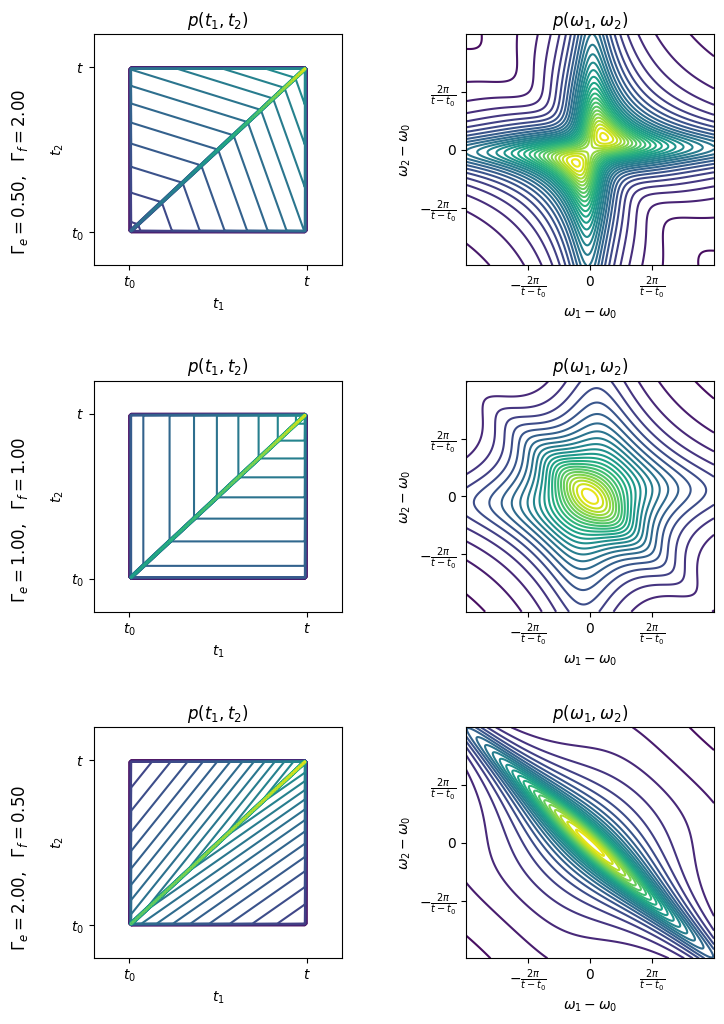
which for gives the probability . The state (164) in the frequency domain is
| (165) |
where
| (166) |
and .
Remark 4
The two-photon state (164) is the time-reversed to the two-photon state emitted spontaneously by the three-level atom in a ladder configuration prepared initially in the state for the case of unidirectional field.
The two-photon state emitted by the three-level atom in a ladder configuration being initially in the state for the multi-directional field was given Scully1997 .
The probability distributions of the optimal state in the time and frequency domains are shown in Figure 1.
VIII.2 Results for a bidirectional field in two-photons state
In this section, we describe the results for the bidirectional field prepared in the two-photon state Loudon2000 ; RMS07
| (167) |
where
| (168) |
and represents the carrier frequency of the -th input field. The field operators in the time domain satisfy the commutation relations
| (169) |
We assume that here we are dealing with the two distinct central frequencies fitting to two different atomic transitions. Then the interaction of the atom with the two unidirectional electromagnetic fields is characterized by the coupling operators:
| (170) |
where and are non-negative coupling constants. In the rotating frame defined by the unitary transformation
| (171) |
we obtain the system Hamiltonian
| (172) |
where and . The probability of the excitation of the state for the atom prepared in the ground state is given by
| (173) |
We used the fact that , where is the conditional vector given by the formula (128). In (173) the operators associated with the absorption of photons have the form
| (174) |
| (175) |
Hence the probability of the two-photon absorption is
| (176) |
In a more general case, the two-photon state field is defined by
| (177) |
where
| (178) |
By referring to the similar arguments to those presented in the previous subsection, which allowed us to determine formula (VIII.1), we obtain for the state (177), the probability of the two-photon absorption of the form
| (179) |
Below we shall present an analysis of the optimal excitation of the atom by the bidirectional field.
Theorem 4
Maximal value of the probability at time reads as follows
| (180) |
and is realized for , , i.e., , and for the two-photon state of the profile
| (181) |
Here the normalization factor has the form
| (182) |
Remark 5
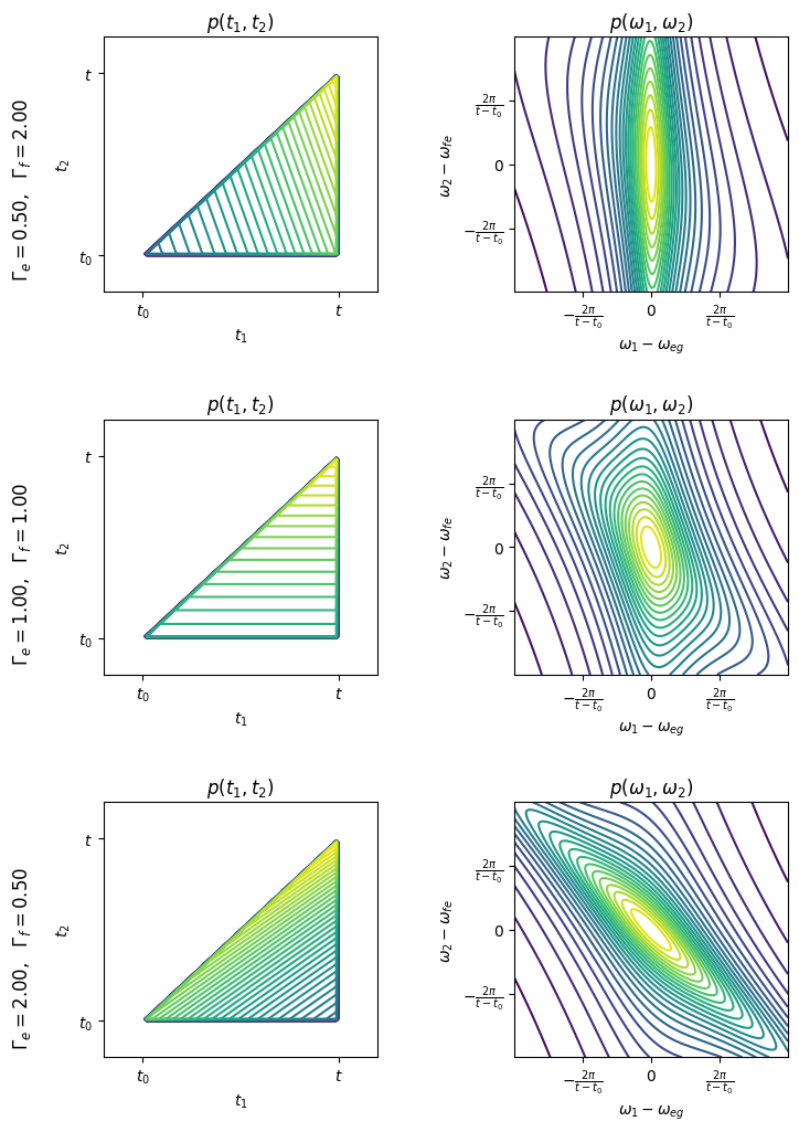
If , then we obtain for the bidirectional field the optimal two-photon state of the form
| (183) |
which for gives the probability . The state (183) in the frequency domain is
| (184) |
where
| (185) |
Remark 6
The two-photon state (183) is the time-reversed to the two-photon state of light emitted spontaneously by the three-level atom in a ladder configuration prepared initially in the state for the case of the bidirectional field.
The probability distributions of the optimal state in the time and frequency domains are shown in Figure 2.
IX Conclusions
In this paper, we have investigated the problem of quantum trajectories for a quantum system interacting with a propagating field prepared in a two-photon state. We have considered two types of the system environment: a unidirectional field and a bidirectional field. Due to temporal correlations of the input field, the evolution of an open system is non-Markovian in this case and given by the sets of coupled filtering or master equations Baragiola12 ; Dong15 ; Zhang2016 ; Dabrowska2019b ; Zhang2019b . The evolution of the system interacting with a traveling field with a definite number of photons is quite complicated, particularly if the photons have different profiles or, even more so, if the photons are entangled. Importantly, instead of considering the sets of coupled filtering equations for operators operators, as in Dong15 ; Zhang2016 ; Dong19 ; Zhang2019b , we have derived the sets of coupled stochastic equations for the conditional vectors. We have determined general analytical formulae for quantum trajectories associated with stochastic counting processes. We have formulated and solved this problem using a collision model. This approach has allowed us to provide a rigorous description of indirect quantum measurement performed on the output field and to the conditional evolution of the quantum system. The recurrence equations for the conditional vectors associated with the counting measurement give us an insight into the problem of excitation of the system and reveal the properties of the output field. We have obtained the recipe for the a posteriori state of an arbitrary quantum system. Using these formulae, one can determine both the conditional as well as unconditional evolution of the open system, and describe the properties of the output field. Our formulae for quantum trajectories can be used to a variety of open systems, including multi-level atoms and resonant cavities.
We have applied the quantum trajectories to derive the formula for the probability of two-photon absorption for a three-level atom in a ladder configuration. The problem of two-photon absorption for propagating light in a two-photon state with a pair of entangled photons is currently being intensively studied by both theorists Schlawin2017 ; Schlawin2021 ; Raymer2021 and experimental physicists Thew2021 ; Thew2022 . We have obtained the analytical formulae describing the excitation of the atom by unidirectional and bidirectional light for an arbitrary two-photon state vector. We have also determined the optimal two-photon state that gives a perfect excitation of the atom. It is worth noting that the optimal state is time-reversed to a two-photon state emitted spontaneously by a three-level atom with a ladder configuration prepared initially at the highest energy level state. The generalisation of these results to the case of a multi-directional field is rather straightforward. An analogous result for the perfect excitation of a two-level atom by the single-photon wavepacket with the raising exponential profile was given in WMSS11 ; Stobinska10a , and examined in the laboratory Scarani2013 ; Leong2016 .
Acknowledgements
Funding information This research was supported partially by the National Science Centre project (Narodowe Centrum Nauki) 2018/30/A/ST2/00837.
Appendix A Proof of Theorem 1
We prove Theorem 1 using the induction method. Assuming that (27) is true for , we can use the property (15) to observe that
| (186) |
The unitary operator acting on the vector gives
| (187) |
The conditional vector from is defined by
where , and is the result of the measurement of (25) at the time . Hence
| (188) |
and it end the proof.
Appendix B Generalization of Theorem 1
Let us consider the two-photon state vector defined in the Hilbert space by the formula
| (189) |
where , given by (22), stands for the normalization factor. Any state of this form can be decomposed as
| (190) |
where is the set of orthogonal functions in , i.e., ), and . We assume here that the phases have been incorporated into the definitions of the basis states and the coefficients are positive.
Theorem 5
The conditional state vector of the input part of the environment (the part of the environment which has not interacted with up to ) and the system , for the initial state
| (191) |
and the measurement of (25), at time has the form
| (192) |
where is the unnormalized conditional vector from the Hilbert space such that
| (193) |
where and the conditional vectors , , from the Hilbert space satisfy the set of coupled recurrence equations:
| (194) | ||||
| (195) | ||||
| (196) |
and initially we have , .
The proof is analogous to the proof of Theorem 1.
Appendix C The interaction operators
Writing down the unitary operator, from Section V in the representation of the photon numbers we get the following operators
| (197) | ||||
| (198) | ||||
| (199) | ||||
| (200) | ||||
| (201) | ||||
| (202) | ||||
| (203) | ||||
| (204) | ||||
| (205) | ||||
| (206) | ||||
| (207) | ||||
| (208) |
Appendix D Proof of Theorem 2
We prove Theorem 2 by the induction. In the first step, we check the initial conditions for , then we assume that (2) is true for , and referring to (15) we get
| (209) |
The unitary operator acting on the vector gives
| (210) |
The conditional vector from is defined by
where , and is the result of the measurement of (83) at the time . Hence
| (211) |
and it ends the proof.
Appendix E Generalization of Theorem 2
Let us consider the two-photon state vector defined in the Hilbert space by the formula (81). By applying the Schmidt decomposition any two-photon state of form (81) can be represented by the expression,
| (212) |
where , , and .
Theorem 6
The conditional state vector of the input part of the environment (the part of the environment which has not interacted with up to ) and the system , for the initial state
| (213) |
and the measurement of (83), is at time is given by
| (214) |
where is the unnormalized conditional vector from the Hilbert space having the form
| (215) |
where , , , and are the conditional vectors from the Hilbert space which satisfy the set of coupled recurrence equations:
| (216) | ||||
| (217) | ||||
| (218) | ||||
| (219) |
and initially , .
The proof is analogous to the proof of Theorem 2.
Appendix F Proof to Theorem 3
Let us introduce . Then the formula (VIII.1) for the two-photon absorption probability has the form
| (220) |
Applying the standard inner product in one can rewrite it as
| (221) |
where and are the element of . In order to maximize the above expression, we have to maximize
| (222) |
The absolute value of the inner product of two vectors is maximized if they are co-linear, hence the optimal is proportional to . After normalisation, we obtain
| (223) |
where is given by (162), and , i.e., .
Appendix G Proof to Theorem 4
Let us introduce . Then the formula (179) for the two-photon absorption probability has the form
| (224) |
This expression can be rewritten using the the standard inner product in the space as
| (225) |
where
| (226) |
The absolute value of the inner product of two vectors is maximized if they are colinear, hence the optimal is proportional to . Hence, after a normalisation, we obtain
| (227) |
where is given by (182). Note that the maximum value of the two-photon absorption is achievable for the resonances and , i.e., .
References
References
- (1) Blow K J, Loudon R, Phoenix S J D and Sheperd, T J: Continuum fields in quantum optics 1990 Phys. Rev. A 42 4102 https://doi.org/10.1103/PhysRevA.42.4102
- (2) Loudon R 2000 The Quantum Theory of Light third edition (Oxford University Press, Oxford)
- (3) Ou Z Y: Temporal distinguishability of an -photon state and its characterization by quantum interference 2006 Phys. Rev. A 74 063808 https://doi.org/10.1103/PhysRevA.74.063808
- (4) Rohde P P, Mauerer W and Silberhorn Ch: Spectral structure and decompositions of optical states, and their applications 2007 New J. Phys 9 91 https://doi.org/10.1088/1367-2630/9/4/091
- (5) Scarani V, Bechmann-Pasquinucci H, Cerf N J, Dusek M, Lütkenhaus N N and Peev M: The security of practical quantum key distribution 2009 Rev. Mod. Phys. 81 1301 https://doi.org/10.1103/RevModPhys.81.1301
- (6) Aaronson S, Arkhipov A: The computation complexity of linear optics. In Proc. 43rd Annual ACM Symposium on the Theory of Computing (STOC11), San Jose, CA, USA, 68 June 2011, New York, NY: Association for Computing Machinery. pp. 333342
- (7) Giovannetti V, Lloyd S and Maccone L Advances in quantum metrology. Nature Photon 5, 222-229 (2011). https://doi.org/10.1038/nphoton.2011.35
- (8) Zhong Z-O, Wang S, Zhan X-H, Yin Z-Q, Chen W, Guo G-C and Han Z-F: Realistic and general model for quantum key distribution with entangled-photon sources 2022 Phys. Rev. A 106 052606 https://doi.org/10.1103/PhysRevA.106.052606
- (9) Raymer M G, Noh J, Banaszek K and Walmsley I A: Pure-state single-photon wavepacket generation by parametric down-conversion in a distributed microcavity 2005 Phys. Rev. A 72 023825 https://doi.org/10.1103/PhysRevA.72.023825
- (10) Cooper M, Wright L J, Söller C and Smith B J: Experimental generation of multi-photon Fock states 2013 Opt. Express 21 5309 https://doi.org/10.1364/OE.21.005309
- (11) Peaudecerf B, Sayrin C, Zhou X, Rybarczyk T, Gleyzes S, Dotsenko I, Raimond J M, Brune, M and Haroche S: Quantum feedback experiments stabilizing Fock states of light in a cavity 2013 Phys. Rev. A 87 042320 https://doi.org/10.1103/PhysRevA.87.042320
- (12) Aljunid S A, Maslennikov G, Wang Y, Dao H L, Scarani V and Kurtsiefer C: Excitation of a Single Atom with Exponentially Rising Light Pulses 2013 Phys. Rev. Lett. 111 103001 https://doi.org/10.1103/PhysRevLett.111.103001
- (13) Yukawa M, Miyata K, Mizuta T, Yonezawa H, Marek P, Filip R and Furusawa A: Generating superposition of up-to three photons for continuous variable quantum information processing 2013 Opt. Express 21 (5) 5529
- (14) Lodahl P, Mahmoodian S and Stobbe S: Interfacing single photons and single quantum dots with photonic nanostructures 2015 Rev. Mod. Phys. 87 347 https://doi.org/10.1103/RevModPhys.87.347
- (15) Reiserer A, Rempe G: Cavity-based quantum networks with single atoms and optical photons 2015 Rev. Mod. Phys 87 1379 https://doi.org/10.1103/RevModPhys.87.1379
- (16) Leong V, Seidler M A, Steiner M, Ceré A and Kurtsiefer Ch: Time-resolved scattering of a single photon by a single atom 2016 Nat. Commun. 7 13716 https://doi.org/10.1038/ncomms13716
- (17) Ogawa H, Ohdan H, Miyata K, Taguchi M, Makino K, Yonezawa H, Yoshikawa J I and Furusawa A: Real-Time Quadrature Measurement of a Single-Photon Wave Packet with Continuous Temporal-Mode Matching 2016 Phys. Rev. Lett. 116 233602 https://doi.org/10.1103/PhysRevLett.116.233602
- (18) Sedziak K, Lasota M and Kolenderski P: Reducing detection noise of a photon pair in a dispersive medium by controlling its spectral entanglement 2017 Optica 4 84 https://doi.org/10.1364/OPTICA.4.000084
- (19) Lodahl P, Mahmoodian S, Stobbe S, Rauschenbeutel A, Schneeweiss P, Volz J, Pichler H and Zoller P: Chiral quantum optics 2017 Nature 541 473 https://doi.org/10.1038/nature21037
- (20) Sun S, Kim H, Luo Z, Solomon G S and Waks E: A single-photon switch and transistor enabled by a solid-state quantum memory 2018 Science 361 (6397) 57 DOI: 10.1126/science.aat3581
- (21) Domokos P, Horak P and Ritsch H: Quantum description of light-pulse scattering on a single atom in waveguides 2002 Phys. Rev. A 65 033832 https://doi.org/10.1103/PhysRevA.65.033832
- (22) Wang Y, Minář J, Sheridan L and Scarani V: Efficient excitation of a two-level atom by a single photon in a propagating mode 2011 Phys. Rev. A 83 063842 https://doi.org/10.1103/PhysRevA.83.063842
- (23) Wang Y, Minář J and Scarani V: State-dependent atomic excitation by multiphoton pulses propagating along two spatial modes 2012 Phys. Rev. A 86 023811 https://doi.org/10.1103/PhysRevA.86.023811
- (24) Chumak O O and Stolyarov E V: Phase-space distribution functions for photon propagation in waveguides coupled to a qubit 2013 Phys. Rev. A 88 013855 https://doi.org/10.1103/PhysRevA.88.013855
- (25) Roulet A, Le H N and Scarani V: Two photons on an atomic beam splitter: Nonlinear scattering and induced correlations 2016 Phys. Rev. A 93 033838 https://doi.org/10.1103/PhysRevA.93.033838
- (26) Shen J T and Fan S: Theory of single-photon transport in a single-mode waveguide. I. Coupling to a cavity containing a two-level atom 2009 Phys. Rev. A 79 023837 https://doi.org/10.1103/PhysRevA.79.023837
- (27) Rephaeli E and Fan S: Stimulated Emission from a Single Excited Atom in a Waveguide 2012 Phys. Rev. Lett. 108 143602 https://doi.org/10.1103/PhysRevLett.108.143602
- (28) Pletyukhov M and Gritsev V: Scattering of massless particles in onedimensional chiral channel 2012 New J. Phys. 14 095028 doi.10.1088/1367-2630/14/9/095028
- (29) Shen Y and Shen J T: Photonic-Fock-state scattering in a waveguide-QED system and their correlation functions 2015 Phys. Rev. A 92 033803 https://doi.org/10.1103/PhysRevA.92.033803
- (30) Konyk W and Gea-Banacloche J: Quantum multimode treatment of light scattering by an atom in a waveguide 2016 Phys. Rev. A 93 063807 https://doi.org/10.1103/PhysRevA.93.063807
- (31) Nysteen A, Trøst Kristensen P, McCutcheon D P S, Kaer P and Mørk J: Scattering of two photons on a quantum emitter in a one-dimensional waveguide: exact dynamics and induced correlations 2015 New J. Phys. 17 023030 DOI 10.1088/1367-2630/17/2/023030
- (32) Fan S, Kocabaş Ş E and Shen J T: Input-output formalism for few-photon transport in one-dimensional nanophotonic waveguides coupled to a qubit 2010 Phys. Rev. A 82 063821 https://doi.org/10.1103/PhysRevA.82.063821
- (33) Rephaeli E and Fan S: Dissipation in few-photon waveguide transport 2013 Photon Res. 1 110 https://doi.org/10.1364/PRJ.1.000110
- (34) Gheri M K, Ellinger K, Pellizzari T and Zoller P: Photon-Wavepackets as Flying Quantum 1998 Bits. Fotschr. Phys. 46 4-5 401 https://doi.org/10.1002/(SICI)1521-3978(199806)46:4/5<401::AID-PROP401>3.0.CO;2-W
- (35) Baragiola B Q, Cook R L, Brańczyk A M and Combes J.: -photon wave packets interacting with an arbitrary quantum system 2012 Phys. Rev. A 86 013811 https://doi.org/10.1103/PhysRevA.86.013811
- (36) Shi T, Chang D E and Cirac J I: Multiphoton-scattering theory and generalized master equations 2015 Phys. Rev. A 92 053834 https://doi.org/10.1103/PhysRevA.92.053834
- (37) Kiilerich A H and Mølmer K: Input-Output Theory with Quantum Pulses 2019 Phys. Rev. Lett. 123 123604 https://doi.org/10.1103/PhysRevLett.123.123604
- (38) Kiilerich A H and Mølmer K: Quantum interactions with pulses of radiation 2020 Phys. Rev. A 102 023717 https://doi.org/10.1103/PhysRevA.102.023717
- (39) Gough J E, James M R, Nurdin H I and Combes J: Quantum filtering for systems driven by fields in single-photon states or superposition of coherent states 2012 Phys. Rev. A 86 043819 https://doi.org/10.1103/PhysRevA.86.043819
- (40) Gough J E, James M R and Nurdin H I: Single photon quantum filtering using non-Markovian embeddings 2012 Phil. Trans. R. Soc. A 370 5408 http://dx.doi.org/10.1098/rsta.2011.0524
- (41) Gough J E, James M R and Nurdin H I: Quantum filtering for systems driven by fields in single photon states and superposition of coherent states using non-Markovian embeddings 2013 Quantum Inf. Process. 12 1469 http://dx.doi.org/10.1007/s11128-012-0373-z
- (42) Dong Z, Zhang G and Amini N H: Quantum filtering for a two-level atom driven by two counter-propagating photons American Control Conference (ACC) 3011-3015 IEEE (2016) http://dx.doi.org/10.1109/ACC.2016.7526105
- (43) Pan Y, Dong D and Zhang G F: Exact analysis of the response of quantum systems to two-photons using a QSDE approach 2016 New. J. Phys. 18 033004 10.1088/1367-2630/18/3/033004
- (44) Song H, Zhang G, Xi Z: Continuous-mode multi-photon filtering 2016 SIAM Journal on Control and Optimization 54(3) 1602 https://doi.org/10.1137/15M102309
- (45) Baragiola B Q and Combes J: Quantum trajectories for propagating Fock states 2017 Phys. Rev. A 96 023819 Quantum filtering for systems driven by fields in single-photon states or superposition of coherent states https://doi.org/10.1103/PhysRevA.96.023819
- (46) Dąbrowska A, Sarbicki G and Chruściński D: Quantum trajectories for a system interacting with environment in a single-photon state: counting and diffusive processes 2017 Phys. Rev. A 96 053819 https://doi.org/10.1103/PhysRevA.96.053819
- (47) Dąbrowska A: Quantum trajectories for environment in superposition of coherent states 2019 Quantum Inf. Process. 18 224 https://doi.org/10.1007/s11128-019-2340-4
- (48) Dąbrowska A, Sarbicki G and Chruściński D: Quantum trajectories for a system interacting with environment in -photon state 2019 Phys. A: Math. Theor. 52 105303 https://doi.org/10.1088/1751-8121/ab01ac
- (49) Dong Z, Zhang G and Amini N H: Quantum filtering for a two-level atom driven by two counter-propagating photons 2019 Quantum Infor. Process. 18 136 https://doi.org/10.1007/s11128-019-2258-x
- (50) Zhang G F: Control engineering of continuous-mode single-photon states: a review 2021 Control Theory and Technology 19 544 https://doi.org/10.1007/s11768-021-00059-7
- (51) Dong Z, Zhang G and Amini N H: Quantum filtering for a two-level atom driven by two counter-propagating photons 2019 Quantum Inf. Process. 18 (5) 136 https://doi.org/10.1007/s11128-019-2258-x
- (52) Dąbrowska A: From a posteriori to a priori solutions for a two-level system interacting with a single-photon wavepacket 2020 J. Opt. Soc. Am. B 37 1240 https://doi.org/10.1364/JOSAB.383561
- (53) Gross J A, Baragiola B Q, Stace T M and Combes J: Master equations and quantum trajectories for squeezed wave packets 2022 Phys. Rev. A 105 023721 https://doi.org/10.1103/PhysRevA.105.023721
- (54) Dąbrowska A: Photon counting probabilities of the output field for a single-photon input 2023 J. Opt. Soc. Am. B 40(5) 1299 https://doi.org/10.1364/JOSAB.487088
- (55) Dąbrowska A and Marciniak M: Stochastic approach to evolution of a quantum system interacting with environment in squeezed number state 2023 Quantum Inf. Process. 22 385 https://doi.org/10.1007/s11128-023-04108-9
- (56) Fischer A K, Trivedi R, Ramasesh V, Siddiqi I and Vuc̆ković J.: Scattering into one-dimensional waveguides from a coherently-driven quantum-optical system 2018 Quantum 2 69 https://doi.org/10.22331/q-2018-05-28-69
- (57) Trivedi R, Fischer K, Xu S, Fan S and Vučković J: Few-photon scattering and emission from low-dimensional quantum systems 2018 Phys. Rev. B 98 144112 https://doi.org/10.1103/PhysRevB.98.144112
- (58) Barchielli A and Belavkin V P: Measurements continuous in time and a posteriori states in quantum mechanics 1991 J. Phys. A: Math. Gen. 24 1495 https://doi.org/10.1088/0305-4470/24/7/022
- (59) Carmichael H 1993 An Open Systems Approach to Quantum Optics (Springer-Verlag, Berlin-Heidelberg)
- (60) Barchielli A: Continual Measurements in Quantum Mechanics and Quantum Stochastic Calculus. In: Attal, S., Alain, Joye, J., Pillet, C-A. (eds.) Lecture Notes Math. 1882, pp. 207-291. Springer, Berlin (2006)
- (61) Gardiner C W and Zoller P 2010 Quantum noise (Springer-Verlag, Berlin-Heidelberg)
- (62) Wiseman H M and Milburn G J 2010 Quantum measurement and control (University Press, Cambridge)
- (63) Hudson R L and Parthasarathy K R: Quantum Ito’s formula and stochastic evolutions 1984 Commun. Math. Phys. 93 301 https://doi.org/10.1007/BF01258530
- (64) Parthasarathy K R 1992 An Introduction to Quantum Stochastic Calculus (Springer Basel AG, Birkhäuser Verlag Basel)
- (65) Gardiner C W and Collet M J: Input and output in damped quantum systems: Quantum stochastic differential equations and the master equation 1985 Phys. Rev. A 31 3761 https://doi.org/10.1103/PhysRevA.31.3761
- (66) Brun T A: A simple model of quantum trajectories 2002 Amer. J. Phys. 70 719 https://doi.org/10.1119/1.1475328
- (67) Gough J E and Sobolev A: Stochastic Schrödinger Equations as Limit of Discrete Filtering 2004 Open Syst. Inf. Dyn. 11 235 https://doi.org/10.1023/B:OPSY.0000047568.89682.10
- (68) Attal S and Pautrat Y: From Repeated to Continuous Quantum Interactions 2006 Ann. Henri Poincaré 7 59 https://doi.org/10.1007/s00023-005-0242-8
- (69) Pellegrini C: Existence, uniqueness and approximation of a stochastic Schrödinger equation: The diffusive case 2008 Ann. Probab. 36 No. 6 2332 https://doi.org/10.1214/08-AOP391
- (70) Pellegrini C and Petruccione F: Non-Markovian quantum repeated interactions and measurements 2009 J. Phys. A Math. Teor. 42 425304 https://doi.org/10.1088/1751-8113/42/42/425304
- (71) Pellegrini C: Existence, uniqueness and approximation of the jump-type stochastic Schrödinger equation for two-level systems 2010 Stoch. Proc. App. 120 Issue 9 1722 https://doi.org/10.1016/j.spa.2010.03.010
- (72) Bouten L, Handel R and James M R: A discrete invitation to quantum filtering and feedback control 2009 SIAM REVIEW 51 239 https://doi.org/10.1137/060671504
- (73) Kretschmer S, Luoma K and Strunz W T: Collision model for non-Markovian quantum dynamics 2016 Phys. Rev. A 94 012106 https://doi.org/10.1103/PhysRevA.94.012106
- (74) Ciccarello F: Collision models in quantum optics 2017 Quantum Measurements and Quantum Metrology 4 53 https://doi.org/10.1515/qmetro-2017-0007
- (75) Altamirano N, Corona-Ugalde P, Mann R B and Zych M: Unitarity, feedback, interactions–dynamics emergent from repeated measurements 2017 New. J. Phys. 19 013035 https://doi.org/10.1088/1367-2630/aa551b
- (76) Gross J A, Caves C M, Milburn G J and Combes J: Qubit models of weak continuous measurements: markovian conditional and open-system dynamics 2018 Quantum Sci. Technol. 3 024005 https://doi.org/10.1088/2058-9565/aaa39f
- (77) Filippov S: Multiparticle Correlations in Quantum Collision Models 2022 Entropy 24 508 https://doi.org/10.3390/e24040508
- (78) Ciccarello F, Lorenzo S, Giovannetti V and Palma G M: Quantum collision models: open system dynamics from repeated interactions 2022 Phys. Rep. 954 1 https://doi.org/10.1016/j.physrep.2022.01.001
- (79) Fang Y L, Ciccarello F and Baranger H U: Non-Markovian dynamics of a qubit due to single-photon scattering in a waveguide 2018 New J.Phys. 20 043035 https://doi.org/10.1088/1367-2630/aaba5d
- (80) Dąbrowska A, Chruściński D, Chakraborty S and Sarbicki G: Eternally non-Markovian dynamics of a qubit interacting with a single-photon wavepacket 2021 New J. Phys. 23 123019 https://doi.org/10.1088/1367-2630/ac3c60
- (81) Scully M O and Zubairy M S 1997 Quantum Optics (Cambridge University Press, Cambridge)
- (82) Stobińska M, Alber G and Leuchs G: Perfect excitation of a matter qubit by a single photon in free space 2009 Euro. Phys. Lett. 86 14007 doi:10.1209/0295-5075/86/14007.
- (83) Schlawin F and Buchleitner A: Theory of coherent control with quantum light 2017 New J. Phys. 19 013009 DOI 10.1088/1367-2630/aa55ec
- (84) Carnio E G, Buchleitner A and Schlawin F: How to optimize the absorption of two entangled photons 2021 SciPost Phys. Core 4 028 DOI:10.21468/SciPostPhysCore.4.4.028
- (85) Raymer M G, Landes T and A. H. Marcus A H: Entangled two-photon absorption by atoms and molecules: A quantum optics tutorial 2021 J. Chem. Phys. 155 081501 https://doi.org/10.1063/5.0049338
- (86) Tabakaev D, Montagnese M, Haack G, Bonacina L, Wolf J P, Zbinden H and Thew R T: Energy-time-entangled two-photon molecular absorption 2021 Phys. Rev. A 103 033701 https://doi.org/10.1103/PhysRevA.103.033701
- (87) Tabakaev D, Djorović A, La Volpe L, Gaulier G, Ghosh S, Bonacina L and Thew R T: Spatial properties of entangled two-photon absorption 2022 Phys. Rev. Lett. 129 183601 https://doi.org/10.1103/PhysRevLett.129.183601
- (88) Pan, Y, Zhang, G.: Scattering of few photons by a ladder-type quantum system. J. Phys. A: Math. Theor. 50 345301 (2017) DOI 10.1088/1751-8121/aa7dee
- (89) Srinivas, M.D., Davies, E.B.: Photon Counting Probabilities in Quantum Optics. Opt. Acta 28:7, 981-996 (1981) https://doi.org/10.1080/713820643