Manifold Learning via Foliations
and Knowledge Transfer

Abstract

Understanding how real data is distributed in high dimensional spaces is the key to many tasks in machine learning. We want to provide a natural geometric structure on the space of data employing a deep ReLU neural network trained as a classifier. Through the data information matrix (DIM), a variation of the Fisher information matrix, the model will discern a singular foliation structure on the space of data. We show that the singular points of such foliation are contained in a measure zero set, and that a local regular foliation exists almost everywhere. Experiments show that the data is correlated with leaves of such foliation. Moreover we show the potential of our approach for knowledge transfer by analyzing the spectrum of the DIM to measure distances between datasets.

1 Introduction

The concept of manifold learning lies at the very heart of the dimensionality reduction question, and it is based on the assumption that we have a natural Riemannian manifold structure on the space of data [40, 19, 41, 14]. Indeed, with such assumption, many geometrical tools become readily available for machine learning questions, especially in connection with the problem of knowledge transfer [9, 45], as geodesics, connections, Ricci curvature and similar [1]. In particular, the fast developing field of Information Geometry [4, 27], is now providing with the techniques to correctly address such questions [26].

However, the practical situation, arising for example in classifying benchmark datasets as MNIST [23], Fashion-MNIST [49] and similar, with CNNs (Convolutional Neural Networks), is generally more complicated and does not allow for such simple description, at least in the cases most relevant for concrete applications, and calls for more sophisticated mathematical modeling.

Machine learning models can be roughly divided into two categories: classifier and generative models. In particular, Deep Learning vision classifier models, via their intrinsic hierarchical structure, offer a natural representation and implicit organization of the input data [31]. For example, the authors of [18] show how a multilayer encoder network can be successfully employed to transform high dimensional data into low dimensional code, then to retrieve it via a “decoder”.

Such organisation strikingly mirrors the one occurring in the human visual perception, as also observed in the seminal work [41], and later an inspiration for the spectacular successful employment of CNNs for supervised classification tasks [24].

In this paper, we want to provide the data space of a given dataset with a natural geometrical structure, and then employ such structure to extract key information. We will employ a suitably trained CNN model to discern a foliation structure in the data space and show experimentally how the dataset our model has been trained with is strongly correlated with its leaves, which are submanifolds of the data space. The mathematical idea of foliation is quite old (see [33, 13] and refs therein); however, its applications in control theory (see [3] and refs therein) via sub-Riemannian geometry and machine learning have only recently become increasingly important [42, 15].

The foliation structure on the data space, discerned by our model, however, is non-standard and presents singular points. These are points admitting a neighbourhood where the rank of the distribution, tangent at each point to a leaf of the foliation, changes. Moreover, in the presence of typical non linearities of the network, as ReLU, there are also non smooth points, thus hindering in such points the smooth manifold structure itself of the leaf. However, we prove that both singular and smooth points are a measure zero set in the data space, so that the foliation is almost everywhere regular and its distribution well defined. As it turns out in our experiments, the samples belonging to the dataset we train our model with are averagely close to the set of singular points. It forces us to model the data space with a singular foliation that we call learning foliation in analogy with the learning manifold. Applications of singular foliations were introduced in connection with control theory [38]; their study is currently an active area of investigation [22]. As we shall show in our experiments, together with their distributions, singular foliations provide with an effective tool to single out the samples belonging to the datasets the model was trained with and at the same time discern a notion of distance between different datasets belonging to the same data space.

Our paper is organized as follows. In Sec. 2, we recap the previous literature, closely related to our work. In Sec. 3, we start by recalling some known facts about Information Geometry in 3.1. Then, in Sec. 3.2 we introduce the data information matrix (DIM), defined via a given model, and two distributions $\mathcal{D}$ and $\mathcal{D}^{\perp}$ naturally associated with it, together with some illustrative examples elucidating the associated foliations and their leaves. In Sec. 3.3 we introduce singular distributions and foliations and then we prove our main theoretical results expressed in Lemma 3.4 and Theorem 3.6. Lemma 3.4 studies the singularities of the distribution $\mathcal{D}$. Theorem 3.6 establishes that the singular points for $\mathcal{D}$ are a measure zero set in the data space. Hence our foliation, though singular, acquires geometric significance. Finally in Sec. 4 we elucidate our main results with experiments. Moreover, we show how the foliation structure and its singularities can be exploited to determine which dataset the model was trained on, and its distance from similar datasets in the same data space. We also make some "proof of concept" considerations regarding knowledge transfer to show the potential of the mathematical singular local foliation and distribution structures in data space.

2 Related Works

The use of Deep Neural Networks as tools for both manifold learning and knowledge transfer has been extensively investigated. The question of finding a low dimensional manifold structure (latent manifold) into high dimensional dataset spaces starts with PCA and similar methods to reach the more sophisticated techniques as in [14, 26], (see also [29] for a description of the most popular techniques in dimensionality reduction and [10] for a complete bibliography or the origins of the subject). Such understanding was applied towards the knowledge transfer questions in [11, 7] and more recently [12]. Though this is not our approach, it is important to mention that one important technique of knowledge transfer is via shared parameters as in [28]. The idea of using techniques of Information Geometry for machine learning started with [4]. More recently, it was used for manifold learning in [26] (see also refs therein). Employing foliations to reduce dimensionality is not per se novel. In [15], the authors introduce some foliation structure in the data space of a neural network, with the aim of approaching dimensionality reduction. In [42], orthogonal foliations in the data space are used to create adversarial attacks, and provide the data space with curvature and other Riemannian notions to analyse such attacks. In [39] invariant foliations are employed to produce a reduced order model for autoencoders. Also, in considering singular points for our foliation, we are led to study the singularities of a neural network. This was investigated, for the different purpose of network expressibility in [16].

3 Methodology

3.1 Information Geometry

The statistical simplex consists of all probability distributions in the form $p(y|x,w)=(p_{1}(y|x,w),\dots,p_{c}(y|x,w))$, where $x$ is a data point, belonging to a certain dataset $D\subset\mathbf{R}^{d}$, divided into $c$ classes, while $w\in\mathbf{R}^{N}$ are the learning parameters [4, 20, 27]. We define the information loss as: $I(x,w)=-\log(p(y|x,w))$ and the Fisher information matrix (FIM) [32] as

$$F(x,w)=\mathbf{E}_{y\sim p}[\nabla_{w}\log p(y|x,w)\cdot(\nabla_{w}\log p(y|x,w))^{T}]$$ (1)

In analogy to (1) we define the Data information matrix (DIM):

$$D(x,w)=\mathbf{E}_{y\sim p}[\nabla_{x}\log p(y|x,w)\cdot(\nabla_{x}\log p(y|x,w))^{T}]$$ (2)

As noted in [26], some directions in the parameter or data space, may be more relevant than others in manifold learning theory. We have the following result [15], obtained with a direct calculation.

Proposition 3.1.

The Fisher information matrix $F(x,w)$ and the data information matrix $D(x,w)$ are positive semidefinite symmetric matrices. Moreover:

$$\begin{array}[]{c}\ker F(x,w)=(\mathrm{span}_{i=1,\ldots,c}\{\nabla_{w}\log p_{i}(y|x,w)\})^{\perp},\\ \\ \ker D(x,w)=(\mathrm{span}_{i=1,\ldots,c}\{\nabla_{x}\log p_{i}(y|x,w)\})^{\perp}.\end{array}$$ (3)

where the orthogonal is taken with respect to the euclidean product. In particular $\mathrm{rank}\ F(x,w)<c$ and $\mathrm{rank}\ D(x,w)<c$.

Notice that $F(x,w)$ is a $N\times N$ matrix, while $D(x,w)$ is a $d\times d$ matrix, where in typical applications (e.g. classification tasks) $N,d>>c$. Hence, both $F(x,w)$ and $D(x,w)$ are, in general, singular matrices, with ranks typically low with respect to their sizes, hence neither $F(x,w)$ nor $D(x,w)$ can provide meaningful metrics respectively on parameter and data spaces. We shall now focus on the data space.

The result (3) suggests to consider the distribution $\mathcal{D}$:

$$\begin{array}[]{c}\mathbf{R}^{d}\ni x\mapsto\mathcal{D}_{x}:=\mathrm{span}_{i=1,\ldots,c}\{\nabla_{x}\log p_{i}(y|x,w)\}\subset T_{x}\mathbf{R}^{d}\end{array}$$ (4)

where we assume the learning parameters $w\in\mathbf{R}^{N}$ to be fixed as $x$ varies. In general a distribution on a manifold $M$ assigns to each point a subspace of the tangent space to $M$ at that point (see [43, 44] for more details), in our case $M=\mathbf{R}^{d}$.

3.2 Distributions and Foliations

Whenever we have a distribution on a manifold $M$, it is natural to ask whether it is integrable. A distribution $\mathcal{C}$ on $M$ is integrable if for every $x\in M$, there exists a connected immersed submanifold $N$ of $M$, with $T_{y}N=\mathcal{C}_{y}$ for all $y\in N$. In other words, the distribution defines at each point the tangent space to a submanifold. Whenever a distribution is integrable, we have a foliation, that is, $M$ becomes a disjoint union of embedded submanifolds called the leaves of the foliation. If $\dim\mathcal{C}_{x}=\dim\mathcal{C}_{y}$ for all $x,y\in M$ we say that the foliation, or the corresponding distribution, has constant rank. Fig. 1 illustrates a constant rank foliation and its orthogonal complement foliation, with respect to the euclidean metric in $M=\mathbf{R}^{3}$ (the ambient space).

Figure 1: Foliations: $\mathcal{L}_{\mathcal{D}}$ and $\mathcal{L}_{\mathcal{D}^{\perp}}$ denote the set of the leaves in distributions $\mathcal{D}$ and $\mathcal{D}^{\perp}$ respectively.

Under suitable regularity hypothesis, Frobenius theorem [43, 44] provides with a characterization of integrable distributions.

Theorem 3.2.

(Frobenius Theorem). A smooth constant rank distribution $\mathcal{C}$ on a real manifold $M$ is integrable if and only if it is involutive, that is for all vector fields $X,Y\in\mathcal{C}$, $[X,Y]\in\mathcal{C}$.

To elucidate this result in Fig. 4 we look at two examples of foliations of 1-dimensional distributions, obtained from the distribution $\mathcal{D}$ in (4) of a neural network trained on the Xor function, with non linearities GeLU and ReLU. Notice that since in both cases $\mathcal{D}$ is 1-dimensional, then it is automatically integrable (bracket of vector fields being zero). We have the following result; the proof is a simple calculation based on the Frobenius Theorem [15].

Proposition 3.3.

Let the notation be as above. For an empirical probability $p$ defined via a deep ReLU neural network the distribution $\mathcal{D}$ in the data space:

$$x\mapsto\mathcal{D}_{x}=\mathrm{span}_{i=1,\ldots,c}\{\nabla_{x}\log p_{i}(y|x,w)\}$$

is locally integrable at smooth points.

We call the foliation resulting from Prop. 3.3 the learning foliation. Its significance is clarified by the following examples.

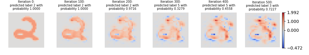
Figure 2: Moving according to $\mathcal{D}$.

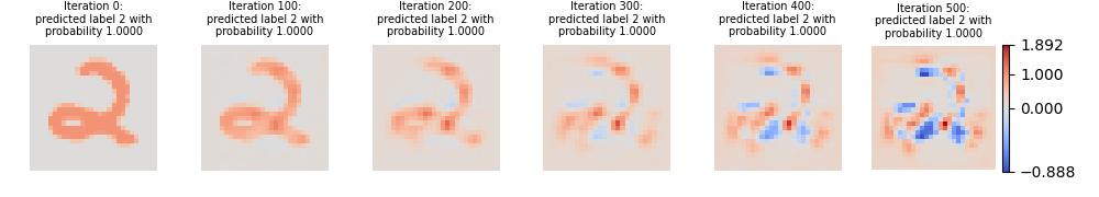
Figure 3: Moving according to $\mathcal{D}^{\perp}$.

As an illustration of the distributions $\mathcal{D}$ and $\mathcal{D}^{\perp}$ (orthogonal computed with respect to the euclidean metric in $M=\mathbf{R}^{d}$), in MNIST, we present Fig. 2 and Fig. 3. We notice that, while moving in $\mathcal{D}$ from one data point , the model predicts a meaningful label, while moving in $\mathcal{D}^{\perp}$, the model maintains high confidence on the label, though not in line with the image. Both Fig. 2 and Fig. 3 were obtained by projecting the same direction on $\mathcal{D}$ and $\mathcal{D}^{\perp}$ at each step. Notice that the phenomena we observe above are due to the fact that the neural network output probabilities are invariant by moving in the kernel of the DIM, that is the distribution $\mathcal{D}^{\perp}$.

For a model with GeLU non linearity however, one can see experimentally that we do not have the involutivity property anymore for the distribution $\mathcal{D}$ (see Table 2). Hence, there is no foliation whose leaves fill the data space, naturally associated to it via Frobenius Theorem. To see this more in detail, we define the space $\mathcal{V}^{D}_{x}$ generated by $\mathcal{D}_{x}$ and the Lie brackets of their generators:

$$\begin{array}[]{c}\mathcal{V}^{D}_{x}=\mathrm{span}\{\nabla_{x}\log p_{i}(y|x,w),[\nabla_{x}\log p_{j}(y|x,w),\nabla_{x}\log p_{k}(y|x,w)],i,j,k=1,\dots,c\}\\ \\ \end{array}$$ (5)

Table 1: Involutivity of the distribution $\mathcal{D}$

Non linearity	dim $\mathcal{D}_{x}$	dim $\mathcal{V}^{D}_{x}$
ReLU	9	9
GeLU	9	44.84
Sigmoid	9	45

In Table 2 we report averages of the dimensions of the spaces $\mathcal{D}_{x}$, $\mathcal{V}^{D}_{x}$ for a sample of 100 points $x\in\mathbf{R}^{d}$. The non involutivity of the distribution is deduced from the fact the dimension increases when we take the space spanned by the distribution and the brackets of its generators. As we can see, while for the ReLU non linearity $\mathcal{D}$ is involutive and we can define the learning foliation, the brackets of vector fields generating $\mathcal{D}$ do not lie in $\mathcal{D}$ for the GeLU and sigmoid non linearities. Consequently, there is no foliation and the sub Riemannian formalism appears more suitable to describe the geometry in this case. We shall not address the question here.

3.3 Singular Foliations

A foliation on a manifold $M$ is a partition of $M$ into connected immersed submanifolds, called leaves. A foliation is regular if the leaves have the same dimension, singular otherwise. Notice that the map $x\mapsto\mathrm{dim}(\mathcal{L}_{x})$, which associates to $x\in M$ the dimension of its leaf $\mathcal{L}_{x}$, is lower semi-continuous, that is, the dimensions of the leaves in a neighbourhood of $x$ are greater than or equal to $\mathrm{dim}(\mathcal{L}_{x})$ [22]. Whenever we have an equality, we say that $x$ is regular, otherwise we call $x$ singular. It is important to remark that, adhering to the literature [22], the terminology singular point here refers to a point that has a neighbourhood where the leaves have non constant dimension. We can associate a distribution to a foliation by associating to each point, the tangent space to the leaf at that point. Such distribution has constant rank if and only if the foliation is regular. Frobenius Theorem 3.2 applies only to the case of constant rank distributions, however, there are results extending part of Frobenius theorem to non constant rank distributions. In [17] and [30], the authors give sufficient conditions for integrability in this more general setting (see [22] for correct attributions on statements and proofs).

In the practical applications we are interested in, foliations may also have non smooth points, that is points where the leaf through the point, belonging to the foliation, is not smooth. For example, Fig. 4 shows a Xor network with ReLU non linearity displaying both singular and non smooth points.

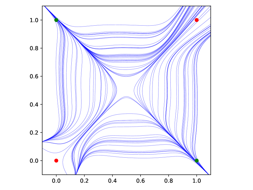
(a) GeLU.

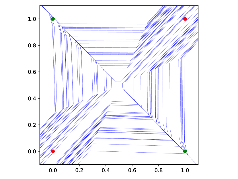
(b) ReLU.

Figure 4: The learning foliation defined by the distribution $\mathcal{D}$ (4) for a Xor network.

The singular point of each picture is in the center, while non smooth points occur only for Xor with ReLU non linearity. As previously stated, this is a degenerate case, where the involutivity and integrability of $\mathcal{D}$ is granted automatically by low dimensionality, though for (b) in Fig. 4, we cannot define $\mathcal{D}$ at non smooth points.

Remark 3.1.

Notice that Frobenius Theorem 3.2 and its non constant rank counterparts, apply only in the smoothness hypothesis, while for applications, i.e. the case of ReLU networks, it is necessary to examine also non smooth foliations. We plan to explore the non smooth setting more generally in a forthcoming paper.

We now want to investigate further the singular points of the distribution $\mathcal{D}$.

Let $N(x)=p(y|x,w)=(p_{1}(y|x,w),\dots,p_{c}(y|x,w))$ denote the output of the neural network classifier and $J_{N}(x)=(\nabla_{x}p_{i}(y|x,w))$ its Jacobian matrix. So $\nabla_{x}p_{i}(y|x,w)$ is the $i$-th row (column) of $J_{N}(x)$. One can see, by the very definition of $\mathcal{D}$ (4), that $\mathrm{rank}\mathcal{D}=\mathrm{rank}J_{N}$. We assume $w$ to be constant, that is we fix our model. Let $P=\mathrm{diagonal}(p_{1}(y|x,w),\dots,p_{c}(y|x,w))$.

From now on we assume $N(x)=\mathrm{Softmax}\circ S(x)$ where $S(x)$ represents the score. Then we have:

$$J_{N}(x)=(P-p^{t}p)J_{S}(x)$$ (6)

where $p=(p_{1}(y|x,w),\dots,p_{c}(y|x,w))$ and $J_{S}(x)$ is the Jacobian of the score.

To study the drop of rank for $\mathcal{D}$ or equivalently for $J_{N}$, let us first look at the kernel of $\left(P-p^{t}p\right)$.

Lemma 3.4.

Let $E_{i}$ denote the vector with the $i$-th coordinate equal to one, and the others equal to zero.

$$\ker(P-p^{t}p)=\mathrm{span}\{(1,\dots,1)\}+\mathrm{span}\{E_{i},~{}\forall i\text{ such that }p_{i}=0\}$$ (7)

Proof.

Let $u\in\mathbf{R}^{c}$. Then $u\in\ker(P-p^{t}p)$ if and only if $p_{i}u_{i}-p_{i}\sum_{k}p_{k}u_{k}=0$. This is equivalent to:

$$p_{i}=0\quad\text{ or }\quad u_{i}-\sum_{k}p_{k}u_{k}=0\iff p_{i}=0\quad\text{ or }\quad\sum_{k}p_{k}(u_{i}-u_{k})=0$$

The inclusion $\supseteq$ is thus straightforward. To get the other inclusion, let $i_{0}$ denote the argmax of $u$. Then, $\sum_{k}p_{k}(u_{i_{0}}-u_{k})$ is a sum of non negative terms; hence to be equal to zero, must be $p_{k}(u_{i_{0}}-u_{k})=0$ for all $k$. Therefore, $u_{k}=u_{i_{0}}$ for all $k$ such that $p_{k}\neq 0$. This is enough to prove the direct inclusion $\subseteq$. ∎

We have the following important observation, that we shall explore more in detail in our experiments.

Observation 3.2.

Lemma 3.4 tells us that the rank of the distribution $\mathcal{D}$ or equivalently of $J_{N}(x)=(P-p^{t}p)J_{S}(x)$ is lower at points in the data space where the probability distribution has higher number of $p_{i}\neq 0$. Clearly the points in the dataset, on which our model is trained, are precisely the points where the empirical probability $p$ is mostly resembling a mass probability distribution. Hence at such points, we will observe empirically an average drop of the values of the eigenvalues of the DIM (whose columns generate $\mathcal{D}$), compared to random points in the data space, as our experiments confirm in Sec. 4. As we shall see, this property characterizes the points in the dataset the model was trained with.

In our hypotheses, since the probability vector $p$ is given by a Softmax function, it cannot have null coordinates. Therefore, Lemma 3.4 states that $\dim\ker(P-p^{t}p)=1$ and that the kernel of $P-p^{t}p$ does not depend on the input $x$. Thus, the drops in rank of $\mathcal{D}$ does not depend on $\ker(P-p^{t}p)$ and can only be caused by $J_{S}(x)$.

Now we assume that the score $S$ is a composition of linear layers and activation functions as follows:

$$S(x)=L_{W_{\ell}}\circ\sigma\circ\dots\circ\sigma\circ L_{W_{1}}$$ (8)

where $\sigma$ is the ReLU non linearity, $L_{W_{i}}$ are linear layers (including bias) and $\ell$ is the total number of linear layers. We denote the output of the $k$-th layer:

$$f_{k}(x)=L_{W_{k}}\circ\sigma\circ\dots\circ\sigma\circ L_{W_{1}}(x)$$

Let us define, for a subset $U$ in $\mathbf{R}^{d}$:

$$Z_{U}=\left\{x\in U\text{ such that }\exists i,~{}x_{i}=0\right\}$$ (9)

Lemma 3.5.

Let $\mathcal{O}$ be the set of points in $M=\mathbf{R}^{d}$, admitting a neighbourhood where the score function $S$ is non constant. Then, the set of singular points of $J_{S}$, the Jacobian of $S$, is a subset of:

$$\bigcup_{k=1}^{\ell-1}f^{-1}_{k}(Z_{f_{k}(M)})\cap\mathcal{O}=\bigcup_{k=1}^{\ell-1}\bigcup_{i=1}^{\dim f_{k}(M)}\left\{x\mid f_{k}(x)_{i}=0\right\}\cap\mathcal{O}$$ (10)

This set is the finite union of closed null spaces, thus of zero Lebesgue measure.

Proof.

A short calculation based on the expression of $S$ (8) gives:

$$\begin{array}[]{lcl}J_{S}(x)&=&W_{\ell}J_{\sigma}\left(f_{\ell-1}(x)\right)W_{\ell-1}J_{\sigma}\left(f_{\ell-2}(x)\right)\dots J_{\sigma}(f_{1}(x))W_{1}\end{array}$$ (11)

Notice that:

$$\left(J_{\text{RELU}}(x)\right)_{i,j}=\begin{cases}\delta_{i,j}&\text{if }x_{i}>0\\ 0&\text{if }x_{i}<0\end{cases}$$ (12)

Hence, the set $Z_{U}$ represents the singular points of $J_{\text{ReLU}}$ on the domain $U$.

If $x_{0}\in\left\{x\mid f_{k}(x)_{i}=0\right\}\cap\mathcal{O}$, then, even if it means making infinitesimal changes to the network weights, there exists a neighborhood of $x_{0}$ such that $(f_{k})_{i}$ is linear on it. Besides, since $x_{0}\in\mathcal{O}$, again, even if it means making infinitesimal changes to the network weights, then $(f_{k})_{i}$ will not be trivial. Thus $\left\{x\mid f_{k}(x)_{i}=0\right\}\cap\mathcal{O}$ is contained in an hyperplane with dimension $<d=\dim M$. ∎

Now we see that singular points occur on a (Lebesgue) measure zero set.

Theorem 3.6.

Let the notation be as above. Consider the distribution $\mathcal{D}$:

$$\mathbf{R}^{d}\ni x\mapsto\mathcal{D}_{x}=\mathrm{span}\{\nabla_{x}p_{i}(y|x,w),\,i=1,\dots c\}$$ (13)

where $p$ is an empirical probability given by Sofmax and a score function $S$ consisting of a sequence of linear layers and ReLU activations. Then, its singular points (i.e. points where $\mathcal{D}$ changes its rank) are a closed null subset of $\mathbf{R}^{d}$ contained in the union of $\ell$ hypersurfaces, where $\ell$ is the number of layers.

Proof.

The singular points of $\mathcal{D}$ coincide, by Lemma 3.4 with the points where $J_{S}$ the Jacobian of $S$ as in (8 changes its rank. By Lemma 3.5 this occurs in the union of $\ell$ hypersurfaces. ∎

We conclude by observing that, as a consequence of the proofs of Lemma 3.5 and Thm 3.6, the singular points of the distribution $\mathcal{D}$ are contained in the non smooth points and such points are contained in a measure zero subset of the data space. Hence, if we restrict ourselves to the open set complementing such measure zero set, we can apply Frobenius Thm to $\mathcal{D}$ to get the learning foliation.

4 Experiments

We perform our experiments on the following datasets: MNIST[23], Fashion-MNIST[49], KMNIST[50] and EMNIST[51], letters only, that we denote with Letters. We also create a dataset that we call CIFARMNIST: it is the CIFAR10 dataset[52] cropped and transformed to be $28\times 28$ gray-scale pictures.

Our neural network is similar to LeNet, with two convolutional layers, followed by a Maxpool and two linear layers with ReLU activation functions, see Fig. 5. This is slightly more general than our hypotheses in Sec. 3.3. The model is then trained on MNIST, reaching $98\%$ of accuracy.

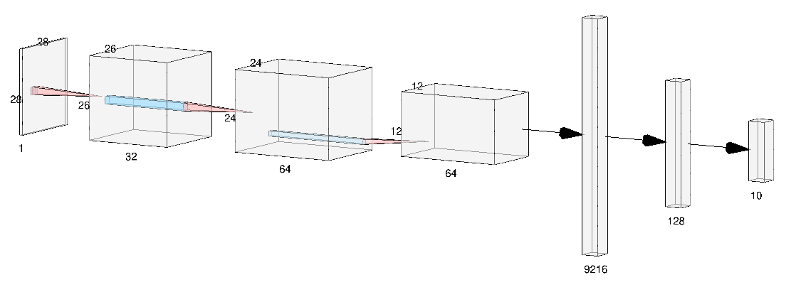
Figure 5: The structure of our CNN - picture created with [25].

In Fig. 6 we compute the Jacobian of the network and we measure its rank by looking at its singular values for 100 sample points in the data space $\mathbf{R}^{784}$ of the MNIST dataset (we normalize the singular values by dividing them by the largest one). The statistical significance of these experiments is detailed in Fig. 7.

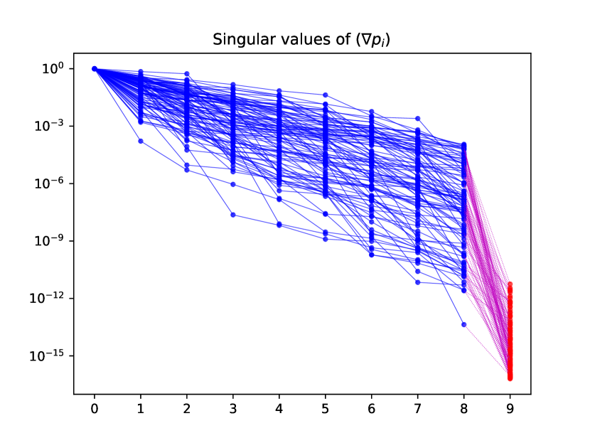
(a) Singular values of $J_{N}$ at 100 data points in MNIST.

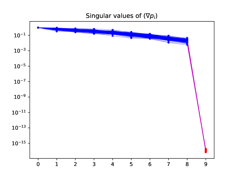
(b) Singular values of $J_{N}$ at 100 random points.

Figure 6: Singular values of the Jacobian $J_{N}$ of the network, normalized by the largest one.

We see clearly that on points in the dataset the singular values of the Jacobian $J_{N}$, are smaller, as we remarked in Obs. 3.2, as a consequence of our Lemma 3.4.

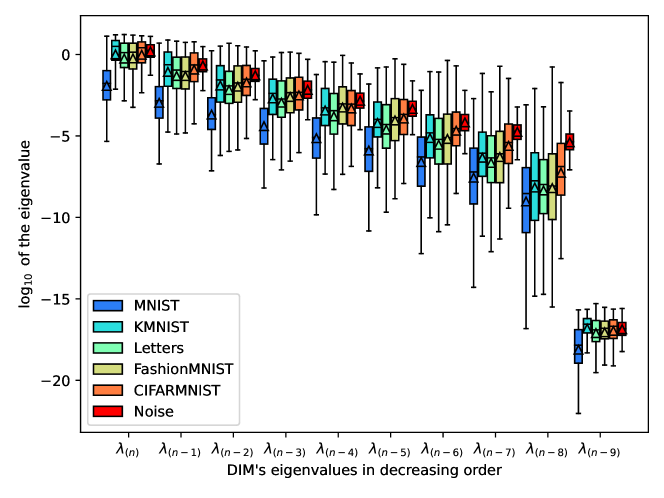
Figure 7: DIM eigenvalues sorted by decreasing order evaluated on 250 points for each dataset.

We report DIM’s eigenvalues (logarithmic scale) for different datasets in Fig. 7. The vertical segment for each eigenvalue and each dataset represents the values for 80% of the samples, while the colored area represents the values falling in between first and third quartile. The horizontal line represents the median and the triangle represents the mean. The points in MNIST, the training dataset, are clearly identifiable by looking at the colored area.

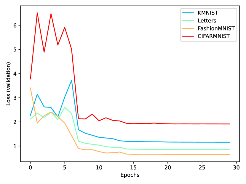
(a) Validation loss.

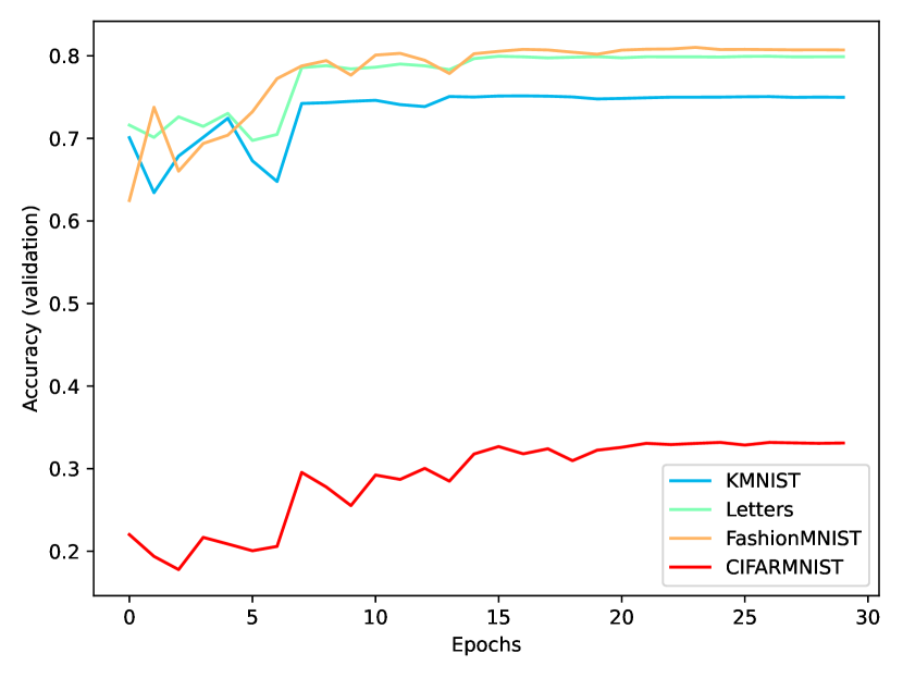
(b) Validation accuracy

Figure 8: Loss and accuracy after transfer learning starting from the weights of a ReLU network trained on MNIST ($98\%$ of accuracy) and retraining only the last linear layer.

We perform a proof of concept knowledge transfer by retraining the last linear layer of our model on different datasets. We report in Table 2 the median of highest and lowest DIM eigenvalues in logarithmic scale, their difference $\Delta$ and validation accuracies after retraining of our CNN. We see a correspondence between the median of the lowest eigenvalue and the validation accuracy, suggesting to explore in future works the relation between DIM, foliations and knowledge transfer.

Table 2: Parameters for Knowledge Transfer (logarithmic scale)

Dataset	Highest evalue	Lowest evalue	$\Delta$	DIM Trace	Val. Acc.
MNIST	-1.78	-8.58	6.70	-1.52	98%
KMNIST	0.49	-7.75	7.76	0.37	75%
Letters	0.11	-7.99	7.82	0.48	80%
Fashion-MNIST	0.14	-8.08	7.76	0.12	81%
CIFARMNIST	0.41	-6.90	6.75	0.27	33%
Noise	0.24	-5.36	5.49	0.27	NA

5 Conclusions

We propose to complement the notion of learning manifolds with the more general one of learning foliations. The (integrable) distribution $\mathcal{D}$, defined via the data information matrix (DIM), a generalization of the Fisher information matrix to the space of data, indeed allows for the partition of the data space according to the leaves of such a foliation via the Frobenius theorem. Examples and experiments show a correlation of data points with the leaves of the foliation: moving according to the distribution $\mathcal{D}$, i.e. along a leaf, the model gives a meaningful label, while moving in the orthogonal directions leads to greater and greater classification errors. The learning foliation is however both singular (drop in rank) and non smooth. We prove that singular points are contained into a set of measure zero, hence making the learning foliation significant in the data space. We show that points in the dataset the model was trained with have lower DIM eigenvalues, so that the distribution $\mathcal{D}$ allows successfully to determine whether a sample of points belongs or not to the dataset used for training. We make such explicit comparison with similar datasets (i.e. MNIST versus FashionMNIST, KMNIST etc). Then, we use the lowest eigenvalue of the DIM to measure the distance between data sets. We test our proposed distance by retraining our model on datasets belonging to the same data spaces and checking the validation accuracy. Our results are not quantitatively conclusive in this regard, but show a great promise as a first step to go beyond the manifold hypothesis and exploiting the theory of singular foliations to perform dimensionality reduction and knowledge transfer.

References

- [1] A. Ache. M. W. Warren Ricci curvature and the manifold learning problem. Advances in Mathematics Volume 342, 21 January 2019, Pages 14-66.
- [2] A. Achille et al. “Task2Vec: Task Embedding for Meta-Learning”. In: Proceedings of the IEEE International Conference on Computer Vision. 2019, pp. 6430–6439.
- [3] A. A. Agrachev, Yu. L. Sachkov, Control theory from the geometric viewpoint. Springer Verlag, 2004.
- [4] S.-I. Amari. “Natural Gradient Works Efficiently in Learning”. In: Neural Comput. 10.2 (Feb. 1998), pp. 251–276.
- [5] Mikhail Belkin, Partha Niyogi, and Vikas Sindhwani. Manifold regularization: A geometric framework for learning from labeled and unlabeled examples. Journal of machine learning research, 7(11), 2006.
- [6] Belkin, M. and Niyogi, P. Laplacian eigenmaps for dimensional- ity reduction and data representation. Neural Comput., 15(6): 1373–1396, 2003.
- [7] Yoshua Bengio. Deep learning of representations for unsupervised and transfer learning. In Proceedings of ICML workshop on unsupervised and transfer learning, pages 17–36. JMLR Workshop and Conference Proceedings, 2012.
- [8] Yoshua Bengio, Aaron Courville, and Pascal Vincent. Representation learning: A review and new perspectives. IEEE transactions on pattern analysis and machine intelligence, 35(8):1798–1828, 2013.
- [9] Stevo Bozinovski, Reminder of the First Paper on Transfer Learning in Neural Networks, 1976, Informatica 44 (2020) 291–302.
- [10] C. J. C. Burges. “Dimension Reduction: A Guided Tour”. en. In: Foundations and Trends in Machine Learning (2010).
- [11] Cook, J., Sutskever, I., Mnih, A., and Hinton, G. E. Visualizing similarity data with a mixture of maps. In AISTATS, JMLR: W&CP 2, pp. 67–74, 2007.
- [12] Nishanth Dikkala, Gal Kaplun, Rina Panigrahy For Manifold Learning, Deep Neural Networks can be Locality Sensitive Hash Functions, https://arxiv.org/abs/2103.06875.
- [13] C. Ehresmann. Structures feuilletees. Proc. Fifth Canad. Math.Congress. - Montreal. (1961), 109-172.
- [14] Fefferman C, Mitter S, Narayanan H. 2016. Testing the manifold hypothesis. J. Amer. Math. Soc. 29(4):983–1049.
- [15] Luca Grementieri and Rita Fioresi. Model-centric data manifold: the data through the eyes of the model. SIAM Journal on Imaging Sciences Vol. 15, Iss. 3 (2022) 10.1137/21M1437056.
- [16] Hanin, Boris Rolnick, David. Deep ReLU Networks Have Surprisingly Few Activation Patterns NeuriPS, (2019).
- [17] R. Hermann. On the Accessibility Problem in Control Theory. In International Symposium on Nonlinear Differential Equations and Nonlinear Mechanics, pages 325–332, Academic Press, New York, 1963.
- [18] Hinton, G. E. and Salakhutdinov, R. R. Reducing the dimensionality of data with neural networks. Science, 313(5786):504-507, 2006.
- [19] Hinton, G. E. and Roweis, S. T. Stochastic Neighbor Embedding. In NIPS 15, pp. 833–840. 2003.
- [20] Jost, J. Riemannian Geometry and Geometric Analysis. Springer, 5th edition, 2008.
- [21] Krizhevsky, A., Sutskever, I., and Hinton, G. E. Imagenet classification with deep convolutional neural networks. In Advances in neural information processing systems, pp. 1097–1105, 2012.
- [22] Sylvain Lavau. A short guide through integration theorems of general- ized distributions. Differential Geometry and its Applications, 2017.
- [23] LeCun, Y., Bottou, L., Bengio, Y., and Haffner, P. Gradient- based learning applied to document recognition. Pro- ceedings of the IEEE, 86(11):2278–2324, 1998.
- [24] LeCun Y., Bengio Y., Hinton G. Deep learning. Nature. 2015; 521(7553): 436-444.
- [25] LeNail, (2019). NN-SVG: Publication-Ready Neural Network Architecture Schematics. Journal of Open Source Software, 4(33), 747, https://doi.org/10.21105/joss.00747
- [26] Ke Sun, Stéphane Marchand-Maillet, An Information Geometry of Statistical Manifold Learning, Proceedings of the 31 st International Conference on Machine Learning, Beijing, China, 2014. JMLR.
- [27] Martens, J. New insights and perspectives on the natu- ral gradient method. Journal of Machine Learning Re- search, 21(146):1–76, 2020.
- [28] Andreas Maurer, Massimiliano Pontil, and Bernardino Romera-Paredes. The benefit of multitask representation learning. Journal of Machine Learning Research, 17(81):1–32, 2016.
- [29] Murphy, Kevin P. Manifold Learning". Probabilistic Machine Learning. MIT Press, 2022. of machine learning research, 4(Jun):119–155, 2003. 1
- [30] T. Nagano. Linear differential systems with singularities and an application to transitive lie algebras. J. Math. Soc. Japan, 18(4):398–404, 1966.
- [31] Olah, C., Mordvintsev, A., and Schubert, L. Feature vi- sualization. Distill, 2017. doi: 10.23915/distill.00007. https://distill.pub/2017/feature-visualization.
- [32] Rao, C. R. Information and accuracy attainable in the estimation of statistical parameters. Bull. Cal. Math. Soc., 37(3):81–91, 1945.
- [33] G. Reeb. Sur les structures feuilletes de codimension 1 et sur un thereme de M.A. Denjoy. Ann. Inst. Fourier, 1961. P. 185-200.
- [34] Roweis S T, Saul L K. Nonlinear dimensionality reduction by locally linear embedding. Science, 2000, 290: 2323–2326
- [35] Hang Shao, Abhishek Kumar, Thomas Fletcher, The Riemannian Geometry of Deep Generative Models, 2018 IEEE/CVF Conference on Computer Vision and Pattern Recognition Workshops (CVPRW), Salt Lake City, UT, USA, 2018, pp. 428-4288, doi: 10.1109/CVPRW.2018.00071.
- [36] Sommer, S. and Bronstein, A. M. Horizontal flows and manifold stochastics in geometric deep learning. IEEE Transactions on Pattern Analysis and Machine Intelli- gence, 2020.
- [37] Peter Stefan. Accessibility and foliations with singularities. Bulletin of the American Mathematical Society, 80:1142–1145, 1974.
- [38] Hector J. Sussmann. Orbits of families of vector fields and integrability of distributions. Transactions of the American Mathematical Society, 180:171–188, 1973.
- [39] Szalai, R. Data-Driven Reduced Order Models Using Invariant Foliations, Manifolds and Autoencoders. J Nonlinear Sci 33, 75 (2023).
- [40] J. B. Tenenbaum. Mapping a manifold of perceptual observa- tions. In Advances in neural information processing systems, pages 682–688, 1998. 1
- [41] Joshua B Tenenbaum, Vin De Silva, and John C Langford. A global geometric framework for nonlinear dimensionality reduction. Science, 290(5500):2319–2323, 2000.
- [42] Eliot Tron, Nicolas Couellan, Stéphane Puechmorel, Canonical foliations of neural networks: application to robustness, abs/2203.00922.
- [43] Tu, L. W. An Introduction to Manifolds. Universitext, Springer, 2008.
- [44] Tu, L. W. Differential Geometry. Universitext, Springer, 2017.
- [45] Weiss, K., Khoshgoftaar, T.M. Wang, D. A survey of transfer learning. J Big Data 3, 9 (2016). https://doi.org/10.1186/s40537-016-0043-6
- [46] Vapnik, V. N. Statistical Learning Theory. Wiley-Interscience, 1998. Journal of Big Data
- [47] Zeng W, Dimitris S, Gu D. Ricci flow for 3D shape analysis. IEEE Trans Pattern Anal Mach Intell, 2010, 32: 662–677
- [48] Zhang Z Y, Zha H B. Principal manifolds and nonlinear dimension reduction via local tangent space alignment. SIAM J Sci Comput, 2005, 26: 313–338
- [49] Xiao, H., Rasul, K., & Vollgraf, R. (2017). Fashion-mnist: a novel image dataset for benchmarking machine learning algorithms. arXiv preprint arXiv:1708.07747.
- [50] "KMNIST Dataset" (created by CODH), adapted from "Kuzushiji Dataset" (created by NIJL and others), doi:10.20676/00000341
- [51] Cohen, G., Afshar, S., Tapson, J., & van Schaik, A. (2017). EMNIST: an extension of MNIST to handwritten letters. Retrieved from http://arxiv.org/abs/1702.05373
- [52] Krizhevsky, Alex, and Geoffrey Hinton. "Learning multiple layers of features from tiny images." (2009): 7.