A Geodetic and Astrometric VLBI Experiment at 22/43/88/132 GHz

Abstract

Extending geodetic and astrometric Very Long Baseline Interferometry (VLBI) observations from traditional centimeter wavebands to millimeter wavebands offers numerous scientific potentials and benefits. However, it was considered quite challenging due to various factors, including the increased effects of atmospheric opacity and turbulence at millimeter wavelengths. Here, we present the results of the first geodetic-mode VLBI experiment, simultaneously observing 82 sources at 22/43/88/132 GHz (K/Q/W/D bands) using the Korean VLBI Network (KVN). We introduced the frequency phase transfer (FPT) method to geodetic VLBI analysis, an approach for calibrating atmospheric phase fluctuations at higher frequencies by transferring phase solutions from lower frequencies. With a 2-minute scan, FPT improved the signal-to-noise ratio (SNR) of most fringes, some by over $100\%$ , thereby enhancing the detection rate of weak sources at millimeter wavebands. Additionally, FPT reduced systematic errors in group delay and delay rate, with the weighted root-mean-squares (WRMS) of the post-fitting residuals decreasing from 25.0 ps to 20.5 ps at the W band and from 39.3 ps to 27.6 ps at the D band. There were no notable differences observed in calibrating atmospheric phase fluctuations at the K band (WRMS = 12.4 ps) and Q band (WRMS = 11.8 ps) with the KVN baselines. This experiment demonstrated that the millimeter waveband can be used for geodetic and astrometric applications with high precision.

1 Introduction

Geodetic and astrometric Very Long Baseline Interferometry (VLBI) observations have made significant contributions to astronomy and geodesy over the past 40 years, particularly in the areas of the terrestrial reference frame (TRF), the celestial reference frame (CRF), and the earth orientation parameters (EOPs) (Sovers et al., 1998). The basic concept of geodetic and astrometric VLBI involves using pairs of radio telescopes to observe the signals of compact extra-galactic objects that emit radiation in the radio frequency regime. By analyzing the differences in the arrival times of the same wavefront between two telescopes, geodetic parameters such as telescope coordinates, positions of celestial objects, and EOPs can be inferred for various scientific and practical applications (Nothnagel, 2019). In addition to the traditional S/X band (2.3/8.4 GHz), multiple frequency bands have recently been employed to enhance the potential of geodetic VLBI observations.

The accuracy of geodetic and astrometric measurements relies on the precision of derived group delays, baseline length, and systematic delay errors. The broadband geodetic VLBI system at 2-14 GHz, known as VLBI Global Observing System (VGOS), has improved the precision of group delays to a few picoseconds (ps; 1 ps = $10^{-12}$ s) (Niell et al., 2018), however, uncompensated systematic errors at the level of 20 ps still dominate the error budget (Xu et al., 2021a). Further efforts are required to calibrate systematic errors originating from tropospheric delay (Petrov, 2024) and source structure (Xu et al., 2022) to achieve the VGOS’s goal of 1 mm position accuracy.

Higher frequency bands offer advantages such as achieving higher-resolution imaging of radio sources, mitigating source structure effects (de Witt et al., 2023), measuring frequency-dependent position shifts in Active Galactic Nuclei (AGN) jets (i.e., core-shift) (Blandford & Königl, 1979; Hada et al., 2011), and reducing interference from scattering (Koryukova et al., 2022) and ionospheric plasma effects (Fomalont et al., 2009). The K band (24 GHz)， X/Ka band (8.4/32 GHz), and Q band (43 GHz) (Lanyi et al., 2010; Charlot et al., 2020) have been used for establishing a multi-frequency International Celestial Reference Frame (ICRF). In the meantime, the $Gaia$ satellite mission realized the first extra-galactic frame at optical wavelengths (Gaia Collaboration et al., 2022). How to realize a fully consistent and integrated multi-waveband celestial reference frame becomes an important issue (Charlot, 2022). In addition, the use of millimeter wavebands for geodesy is valuable for determining the station coordinates of antennas without receivers operating at lower frequencies.

The independent geodetic VLBI programs operating at different frequencies may have astrometric limitations in detecting the core-shift in most ICRF sources (Petrov, 2024). As frequency increases, the signal-to-noise ratio (SNR) of VLBI fringes is affected by decreased flux densities of sources, shorter coherence times, increased atmospheric absorption, and higher receiver temperatures, limiting the precision of group delays at millimeter wavelengths. The single K band observation also has difficulty in calibrating the ionospheric delay (Lanyi et al., 2010).

The Korean VLBI Network (KVN) has the capability of simultaneously observing at multiple frequencies (Han et al., 2013), including K band at 18-26 GHz, Q band at 35-50 GHz, W band at 85-116 GHz, and D band at 125-142 GHz. A similar K/Q/W band system is being developed globally (Dodson et al., 2023). This kind of system is particularly useful for extending the coherence time at millimeter wavelengths using the frequency phase transfer (FPT) technology (Rioja & Dodson, 2020). Specifically, it achieves this by calibrating the tropospheric phase at higher frequencies through transferring phase solutions from lower frequencies. This enables the observation of more sources and facilitates the measurement of core shift effects using source-frequency phase-referencing (SFPR) astrometry (Rioja et al., 2015; Jung et al., 2015). The global K/Q/W band system may also benefit the ICRF by employing geodetic and astrometric VLBI across a broad frequency range from 20 to over 100 GHz. This approach offers several advantages: 1) simultaneous multi-frequency investigation of core shift effects and source structures; 2) monitoring numerous ICRF source images with resolutions of a few tens of microarcseconds; 3) overcoming limitations in group delay precision at millimeter wavelengths through very broad bandwidth synthesis.

In this paper, we present the first geodetic VLBI observation at 22/43/88/132 GHz simultaneously using the KVN as a pilot experiment for future broad bandwidth synthesis from 20 to over 100 GHz.

2 Observations and general DATA ANALYSIS

Table 1: KVN geodetic observation in 2021 December 07/08

Band	Frequency	Polarization	Channel	Number of	Scheduled	Scheduled
ID	(MHz)		bandwidth (MHz)	channel	scans	observables
K	21984	RCP	512	1	485	1455
Q	42620	LCP	512	1	485	1455
W	87936	LCP	512	1	485	1455
D	131904	LCP	512	1	485	1455

We conducted the first geodetic and astrometric VLBI experiment observed at K/Q/W/D bands (22/43/88/132 GHz) simultaneously using the KVN under the East Asian VLBI Network (EAVN) (Akiyama et al., 2022) program a2129a . The KVN consists of three 21-m antennas: KVN-Yonsei (KYS), KVN-Ulsan (KUS), and KVN-Tamna (KTN), with baseline lengths ranging from 305 to 476 km. We used a 24-hour track for the session from 2021-Dec-07/15:25:00 to 2021-Dec-08/15:25:00. The received signals were recorded with four 512 MHz base-band channels (BBCs) and recorded right (for K band) or left (for Q/W/D bands) circularly polarized signals with Nyquist sampling and 2 bits per sample for a total sampling rate of 8 Gbps. A summary of the observation is listed in Table 1.

2.1 Scheduling

There are a few known sources at W and D bands that can be used for geodetic VLBI observations. Fortunately, the Multi-frequency AGN Survey with the KVN (MASK) project (Jung, 2018) provided suitable candidates for this geodetic session. MASK is a simultaneous multi-frequency VLBI fringe detection survey utilizing the FPT technique for $\sim$1533 AGN samples from the KVN single dish survey (Lee et al., 2017) with a bandwidth of 64 MHz for each K/Q/W/D band (1 Gbps in total) and a 30-min scan for each source. MASK has detected hundreds of AGNs at W and D bands using the phase self-calibration or the FPT technique (Jung et al. in preparation). We selected a candidate catalog with 125 sources, all of which were detected at K/Q/W/D bands with MASK and included in the ICRF3 K band catalog (Charlot et al., 2020).

Observation scheduling was performed using the NASA VLBI scheduling program SKED (Gipson, 2018). We used a 2-min scan for each source with 8 Gbps (2 Gbps per band) recording mode (with low system noise temperature in winter), which has comparable sensitivity to the MASK project (30-min scan and 1 Gbps recording mode). The best 80 targets were selected automatically by SKED. During the geodetic observations, we also included five $\sim$8-min “phase-referencing blocks” for two source pairs: 4C39.25$\sim$0945+408 (4.5^∘ separation) and 2136+141$\sim$2150+173 (4.5^∘ separation). For each “phase-referencing block”, we switched between the source pairs for 3 cycles with a switching time of $\sim$20 s and on-source time of 60 s for each target. (The results of the phase-referencing blocks are not within the scope of this paper and will be reported elsewhere.) The sources 4C39.25 and 2136+141 were included in the best 80 targets, and the sources 0945+408 and 2150+173 were added manually. All 82 sources are listed in APPENDIX A.

A total of 485 scans were scheduled for each KVN baseline using SKED. Since the KVN has its own field system supporting the NRAO VLBI scheduling program SCHED, the observing scans from SKED were modified to SCHED format.

2.2 Correlation and Fringe fitting

The observations were correlated using the DiFX software correlator (Deller et al., 2011) in Daejeon, South Korea. The output of the correlator was converted to Mark 4 format in order to be compatible with the Haystack Observatory Processing System (HOPS) suite of programs (Whitney et al., 2022) and converted to FITS format for imaging with NRAO Astronomical Image Processing System (AIPS) (Greisen, 2003).

The HOPS main tool, fourfit, was used to estimate group and phase delays, phase, delay rate, and cross-correlation amplitude for each observation using the Mark 4 data. As the hardware phase calibration system to cover the entire frequency range of KVN (18 - 142 GHz) is under development, we implemented manual phase calibration through a single scan of the bright source OJ287, to align the delays and phases among different frequency bands. Contrary to the standard practices in geodetic VLBI, we introduced the utilization of FPT to address the effects of atmospheric turbulence in millimeter wavebands. This method is elucidated in Section 3. A database in vgosDb format (Bolotin et al., 2016) was finally produced in three steps: “vgosDbMake” produced the skeleton database for all observables (version 1); “vgosDbCalc” added the apriori values and partial derivatives (version 2), and “vgosDbProcLogs” added meteorological information (version 3; no cable cal in KVN log file)(Bolotin et al., 2014).

2.3 Geodetic data analysis

The geodetic analysis was conducted using the nuSolve program (Bolotin et al., 2014). This program operates on the vgosDb database to perform least-squares estimation of various geodetic, geophysical, astronomical, and instrumental parameters. We disassembled the database into individual bands (e.g., K, Q, W, D) and dual-bands (e.g., Q/K, W/K, D/K) by manually editing the “wrapper” file in the vgosDb database.

Obtaining the final geodetic estimate utilized multiple steps proceeding from least precise to most precise. The detailed steps can be found in the User Guide of nuSolve and Niell et al. (2021). External files containing a priori information are used in the analysis, such as updated station coordinates from the multi-epoch EAVN geodetic observations (Xu et al., 2021b), source positions from the ICRF3 K band catalog (Charlot et al., 2020), and earth rotation parameters from the VLBI solution provided by NASA Goddard Space Flight Center (GSFC). The group delays with the single 512 MHz channel in our data are unambiguous. We start with simple parameterization, only clock shifts and rates, and perform an analysis of the group delays. At this stage, we use the KYS station as the clock reference and have not identified any clock breaks at any of the stations. Then we add zenith delays and station positions to the list of estimated parameters.

Also, we test ionospheric corrections for dual-frequency (Q/K, W/K, D/K) band data. Usually, geodetic VLBI uses multi-frequency channels for each frequency band, i.e., the bandwidth synthesis technique, to improve the group-delay measurement precision. In this case, an “effective frequency” is calculated and assigned to ionosphere group delays as the approximate reference frequency (Bohm & Schuh, 2013). We calculated the central frequencies of each band (22240 MHz for K band, 42876 MHz for Q band, 88192 MHz for W band, 132160 MHz for D band) as the effective frequency and used them latter in ionospheric calibration.

Time-varying models of clock and tropospheric parameters are introduced in the latter stage. They are modeled as continuous piece-wise linear (PWL) functions with incremental rates. For such a PWL model, the estimated values are, for each parameter, an initial value and rate for the first interval and a new rate for each of the successive equal-duration intervals. The results reported in the remainder of this paper are based on a PWL interval of 30 min for the troposphere and 60 min for the clock. The daily averaged atmospheric gradients (MacMillan, 1995) are estimated with constraints in this independent solution. In the last stage of data processing, additional parameters such as the rate of Earth rotation and angles of nutation are included. We also re-weight the observations by examining the additive noise required to achieve a chi-squared per degree of freedom (chi2pdof) of approximately 1. Any post-fit delay residuals greater than 3.5 times their re-weighted uncertainty are marked for exclusion. We iterate through the estimation, re-weighting, and outlier-check sequence until no outliers are detected, resulting in the final solution. To efficiently compare results from different frequency bands and/or parameters, we use the script mode with nuSolve (Bolotin et al., 2023).

3 Application of FPT in geodetic VLBI

The inherent challenges of geodetic VLBI in millimeter wavebands, such as sensitivity, can be effectively addressed due to the impressive performance of the KVN telescopes (Lee et al., 2014), characterized by their high aperture efficiency, precise pointing accuracy, receivers with low noise temperature, wide-band digital backend, and rapid slewing speed. Of particular significance is the telescopes’ ability to operate at multiple frequencies, which enables us to mitigate atmospheric phase fluctuations using the FPT method. In the FPT method, high-frequency (target frequency) observations are calibrated using scaled solutions obtained from a lower, more easily manageable frequency (Jung et al., 2011; Rioja & Dodson, 2020).

The majority of mm-VLBI observations serve imaging purposes, wherein the rapid nonlinear phase (atmospheric phase fluctuations) is usually estimated per scan using self (on-source) detections from a single reference station to other stations (Blackburn et al., 2019). The correlated signal must have a high SNR so that the atmospheric phase can be estimated on a short timescale (a few seconds). Therefore, this method is limited to using bright sources or using a high-sensitivity station as the phase reference. In addition, it is difficult to distinguish nonlinear atmospheric phase from the linear phase drift due to delay rate, and can lead to the loss of frequency-dependent information in the phases. The FPT method can be effectively employed to overcome these limitations, either simultaneously or through fast frequency switching.

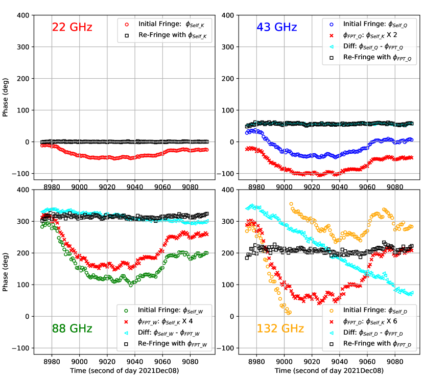
Figure 1: Comparison atmospheric phase fluctuations with self detection ($\phi_{Self}$) and FPT ($\phi_{FPT}$) method using a strong source 3C279 on KTN-KYS baseline. The four panels represent distinct frequency bands. The 2$\pi$ ambiguity of phase is ignored for clarity.

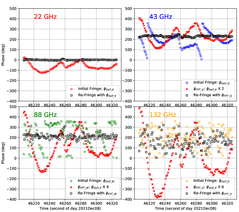
Figure 2: Same as Figure 1, but for a weaker source 0642$+$449.

We effectively employed the FPT method using the packets HOPS for geodetic data, drawing from the guidance provided in the fourfit user’s manual and a tutorial (Fish, 2015). This implementation involved the following steps:

• Initiating fringe fitting using the fourfit program and employing the alist program to track the fringe phase, SNR, and other information for each observation, leading to the creation of a corresponding text file.

• Employing the fringex program to segment data from a single scan time ($\sim$2 min) into a few seconds. This step utilized the aforementioned text file (alist) as input and provided atmospheric phase fluctuations using self detection at each bands (e.g., $\phi_{Self\_K}$, $\phi_{Self\_Q}$, $\phi_{Self\_W}$, and $\phi_{Self\_D}$). Choosing a reference station and an appropriate cadence for segmented phases is crucial; it should be short enough to capture the atmospheric phase fluctuations while maintaining enough SNR. In this experiment, we used KYS as the reference station and examined cadences of 1 second, 3 seconds, 5 seconds, and 10 seconds. Subsequently, we selected the smallest cadence with an SNR exceeding 10. Given the high SNRs in the K band, $\sim$90$\%$ of the scans adopted a 1-second cadence. However, for a small number of weaker scans with an SNR below 10 at the 10-second cadence, we refrained from applying FPT to prevent the potential deterioration of results.

• Calculating atmospheric phase fluctuations at higher frequencies by transferring phase solutions from a lower frequency (i.e., K band), based on frequency ratios. As illustrated in Table 1, the frequency ratios are 1.93 (approximately equal to 2) for Q/K bands, 4 for W/K bands, and 6 for D/K bands, resulting in $\phi_{FPT_{Q}}=\phi_{Self_{K}}\times 2$, $\phi_{FPT_{W}}=\phi_{Self_{K}}\times 4$, and $\phi_{FPT_{D}}=\phi_{Self_{K}}\times 6$. We have applied phases from one polarization (LCP of K band) to the other (RCP of Q/W/D band), as atmospheric phases remain unaffected by polarization.

• Within the HOPS framework, the solutions were based on baselines. We designated KYS as the reference station and “viewed” the atmospheric phases ($\phi_{Self\_K}$, $\phi_{FPT\_Q}$, $\phi_{FPT\_W}$, $\phi_{FPT\_D}$) originating from KUS and KTN stations. Finally, we integrated this “ad hoc” phase information into fourfit and re-performed the process of fringe fitting.

As shown in Figure 1 and 2, the FPTed phases exhibit close agreement with the trends observed in self detected phases at each K/Q/W/D bands. The clear linear phase differences ($Diff:\phi_{Self}-\phi_{FPT}$ in Figure 1) between self detection and FPT method indicate the different delay rates. In Table 2, it is noteworthy that the fringe quality (“Qcodes”) of FPT-derived detection is comparable to those of self-detection. The term “Qcodes” represents the fringe quality code as defined by HOPS-fourfit, where higher Qcodes indicate better quality. Subsequent to the application of FPT, the proportion of all usable observables with Qcodes of 9 has improved from 79$\%$ to 99$\%$, characterized by heightened SNR and improved delay/rate precision. The improvements in group delay and rate accuracy are presented in Section 4. After applying FPT, the presence of phase differences among different bands in Table 2 necessitates further investigation through precise instrumental phase calibration. However, their influence on group delay and delay rate measurements is negligible in the following analysis.

Table 2: The fringe information with observables in Figure 1 and 2

Source	Band	Frequency	Atmospheric phase	Qcodes	SNR	Phase	Group delay	Delay rate
	ID	(MHz)	calibration			(degree)	precision (ps)	precision (ps/s)
3C279	K	21984	NO	8	5108.0	-36.7	2.1E-01	4.0E-5
			$\phi_{Self\_K}$	9	5233.1	0.1	2.1E-01	3.9E-5
	Q	42620	NO	7	3853.5	-17.3	2.8E-01	2.8E-5
			$\phi_{Self\_Q}$	9	4256.0	-0.1	2.5E-01	2.5E-5
			$\phi_{FPT\_Q}$	9	4253.4	56.5	2.5E-01	2.5E-5
	W	87936	NO	5	740.7	158.0	1.5E+00	7.1E-5
			$\phi_{Self\_W}$	9	1121.8	0.3	9.6E-01	4.7E-5
			$\phi_{FPT\_W}$	9	1120.3	-45.5	9.6E-01	4.7E-5
	D	131904	NO	5	275.1	-75.7	3.9E+00	1.3E-4
			$\phi_{Self\_D}$	9	394.5	1.1	2.7E+00	8.8E-5
			$\phi_{FPT\_D}$	9	392.3	-152.8	2.7E+00	8.9E-5
0642+449	K	21984	NO	6	349.7	-64.1	3.1E+00	5.9E-4
			$\phi_{Self\_K}$	9	412.2	0.3	2.6E+00	4.9E-4
	Q	42620	NO	5	131.9	-175.0	8.2E+00	8.2E-4
			$\phi_{FPT\_Q}$	9	254.2	-129.9	4.2E+00	4.3E-4
	W	87936	NO	9	18.7	-17.8	5.7E+01	2.8E-3
			$\phi_{FPT\_W}$	9	37.2	-150.0	2.9E+01	1.4E-3
	D	131904	NO	0	5.3	-127.5	2.0E+02	6.5E-3
			$\phi_{FPT\_D}$	9	9.2	156.7	1.2E+02	3.8E-3

4 Results

The weather conditions were clear during the observation period, with median system temperature (Tsys) ranges as follows: 87-131 K for the K band, 96-103 K for the Q band, 189-193 K for the W band, and 186-270 K for the D band at the three KVN stations. These favorable conditions have led to excellent detection (SNR $>=$ 7), with the detection rate of 99.8$\%$ at K band, 99.8$\%$ at Q band, 95.5$\%$ at W band (or 96.3$\%$ with FPT), and 68.2$\%$ (or 70.9$\%$ with FPT) at D band for 485 scans on KYS-KTN baseline. However, the Q band data from the KUS station exhibited a rare lower SNR compared to other stations, for unknown instrumental reasons at this time. Therefore, we didn’t use the Q band data of KUS station in the final results.

4.1 The group delay and delay rate measurements at 22/43/88/132 GHz

As shown in Figure 3, FPT improved the SNR of most fringes, some by more than 100$\%$ with a 2-minute scan length, resulting in a higher detection rate (over 100 observables) for weak sources at millimeter wavebands. Note that most sources in this experiment are bright. Detection can be further improved in experiments with weaker sources and longer scan lengths.

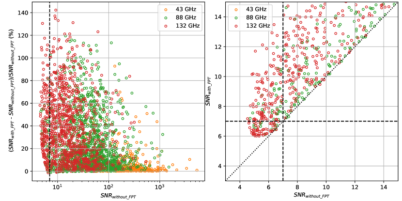
Figure 3: Comparison of the SNR with and without FPT within a 2-minute scan length. The left figure shows the percentage increase in SNR after using FPT, and the right figure compares the SNR of weak sources (SNR $<$ 15). The dashed lines indicate the fourfit detection limit (SNR $=$ 7). For clarity, the results with an SNR below 6 using FPT are not shown.

The theoretical uncertainties of group delays produced by fourfit are calculated using $\sqrt{12}/(2\pi$*SNR*512 MHz) for the single 512 MHz channel data. Figure 4 shows the measurement noise of group delays on KYS-KTN baseline for each band. The median formal errors of group delays are 3.5 ps at K band, 5.0/4.7 ps at Q band, 22.5/19.5 ps at W band, and 49.7/43.0 ps at D band without/with FPT. Similarly, the median formal errors of delay rates are 6.6E-4 ps/s at K band, 5.0E-4/4.8E-4 ps/s at Q band, 1.1E-3/9.8E-4 ps/s at W band, and 1.7E-3/1.5E-3 ps/s at D band without/with FPT.

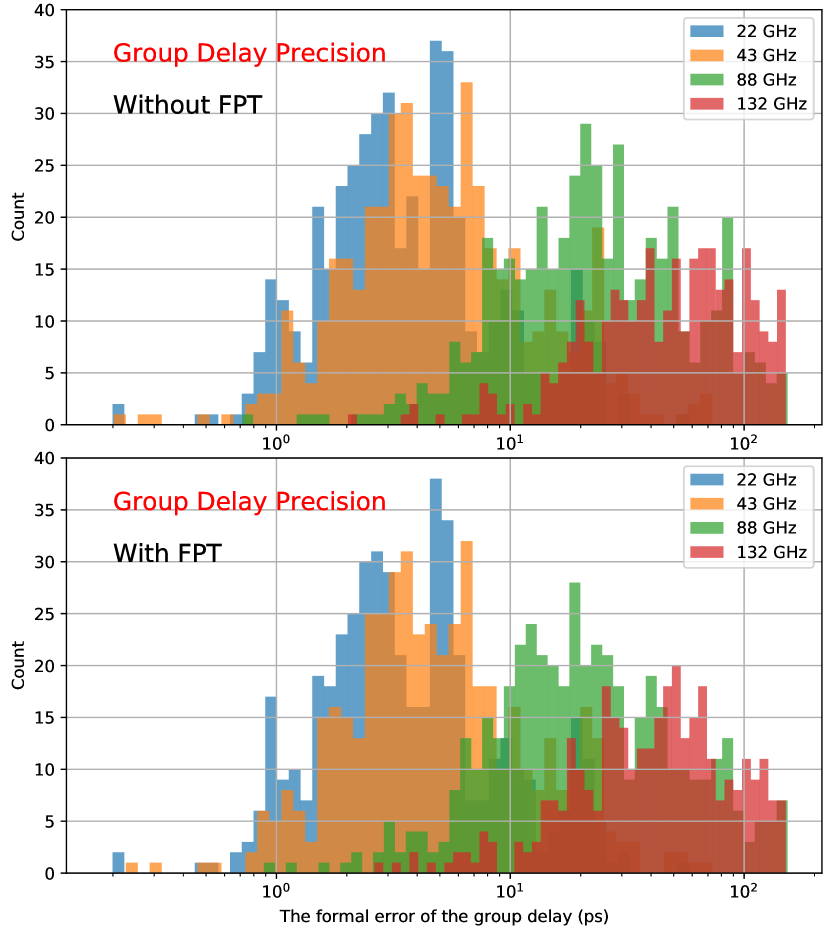
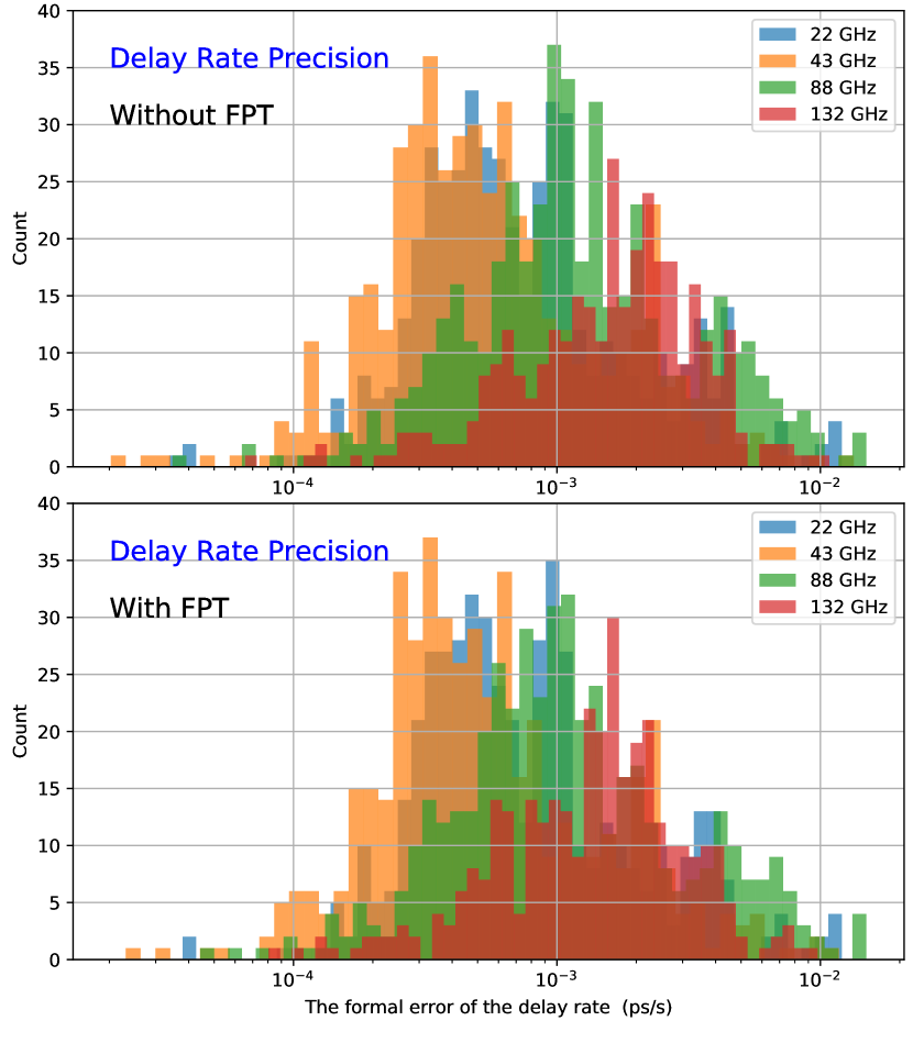
Figure 4: The histogram of measurement noise for group delay and delay rate produced by fourfit on the KYS-KTN baseline. Different bands are represented by different colors.

The closure group delay for a triangle of three stations simultaneously observing the same source is given by the sum of the three baseline group delays going around a closed loop of the triangle (Xu et al., 2016). In this summation, the effects of station-based delays (tropospheric delays, ionospheric delays, station position errors, station thermal deformation errors, clock offset errors, cable delay errors, EOP errors, errors from pointing offsets, and so on) cancel exactly. The major error terms at centimeter wavebands that remained in the closure quantities, the so-called nonclosing errors, are source structure and measurement noise (Anderson & Xu, 2018). However, in millimeter wavebands, atmospheric phase fluctuations become significant within seconds and differ at each triangle baseline, leading to errors in baseline-dependent fringe fitting when employing a 2D linear model (phase vs. time, phase vs. frequency) over a 2-minute scanning duration. As a result, uncalibrated atmospheric phase fluctuations will contribute to non-closure errors in millimeter wavebands when using HOPS-fourfit.

Figure 5 and Table 3 show the closure observables in the KVN triangle baseline (KTN-KUS-KYS, with SNR $>=$ 7 on each single baseline). With the exception of notable errors in the Q band attributed to the KUS station issue, the weighted standard deviations of closure group delays are 3.7 ps at K band, 19.9/15.7 ps at W band, and 47.2/36.7 ps at D band without/with FPT. These values commendably align with their corresponding formal errors, as illustrated in Figure 4. Moreover, the application of FPT noticeably enhances the accuracy of the closure group delays at the W and D bands. Similarly, the weighted standard deviations of closure delay rates are 1.7E-3 ps/s at K band, 3.5E-2/1.3E-3 ps/s at W band, and 6.1E-2/1.3E-3 ps/s at D band without/with FPT. And the weighted standard deviations of closure phases are 2.1^∘ at K band, 24.4^∘/3.1^∘ at W band, and 55.9^∘/4.4^∘ at D band without/with FPT. The FPT method significantly enhances the closure delay rate and closure phase by over an order of magnitude at the W and D bands.

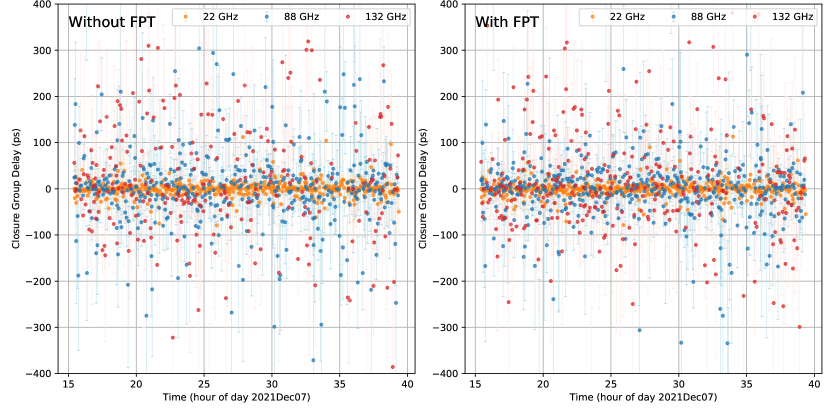
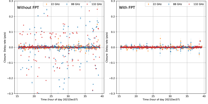
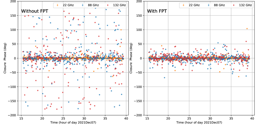
Figure 5: The closure group delay, closure delay rate, and closure phase in the KVN triangle baseline (KTN-KUS-KYS), with different frequency bands represented by dots of different colors. Up panels: closure group delay without/with FPT; Middle panels: closure delay rate without/with FPT; and Bottom panels: closure phase without/with FPT. The 43 GHz result is not presented and has large uncertainties due to the low SNR issues on KUS station.

Table 3: Statistics of the closure observables in KVN triangle baselines

Band	Frequency	Atmospheric phase	Number of	Group delay	Group delay	Delay rate	Delay rate	Phase	Phase
ID	(MHz)	calibration	triangle	WMean (ps)	WRMS (ps)	WMean (ps/s)	WRMS (ps/s)	WMean (∘)	WRMS (∘)
K	21984	NO	481 (99.2%)	-0.2$\pm$1.7	3.7	-6.1E-5$\pm$7.9E-5	1.7E-3	-0.1$\pm$0.1	2.1
		$\phi_{Self\_K}$	481 (99.2%)	-0.2$\pm$0.2	3.6	-2.3E-4$\pm$1.1E-4	2.6E-3	-0.2$\pm$0.1	2.2
W	87936	NO	437 (90.1%)	1.4$\pm$1.0	19.9	1.1E-3$\pm$1.7E-3	3.5E-2	-2.4$\pm$1.2	24.4
		$\phi_{FPT\_W}$	454 (93.6%)	1.8$\pm$0.7	15.7	-3.5E-5$\pm$6.2E-5	1.3E-3	-0.7$\pm$0.2	3.1
D	131904	NO	254 (52.4%)	0.7$\pm$3.0	47.2	1.9E-2$\pm$3.8E-3	6.1E-2	9.4$\pm$3.5	55.9
		$\phi_{FPT\_D}$	301 (62.1%)	2.1$\pm$2.1	36.7	1.4E-4$\pm$7.7E-5	1.3E-3	0.2$\pm$0.3	4.4

4.2 The tropospheric and ionospheric effects with KVN

The path delay of radio waves caused by the troposphere is one of the major error sources. Modeling the tropospheric delay is generally divided into hydrostatic and wet parts, each of which is the product of the zenith delay and the corresponding mapping function dependency on elevation angle (Bohm & Schuh, 2013). In nuSolve, the zenith hydrostatic delay (ZHD) is modeled as a function of the surface pressure, and the zenith wet delay (ZWD) is calculated with the relative humidity and temperature at the surface (Saastamoinen, 1972; Davis et al., 1985). However, the uncertainty of ZWD model is far larger than ZHD model due to high spatial and temporal variability and unpredictability of the amount of water vapor. Therefore, the residual ZWD is then parameterized as a PWL function of time (e.g., the interval of 30 min in this experiment) in the data analysis. We compared the solutions with two different sets of priori ZHD+ZWD: one using meteorological data (pressure, relative humidity, temperature) from the station’s log files and the other using a constant value from the standard model in nuSolve. The use of meteorological data resulted in increased weighted root-mean-squares (WRMS) of the post-fitting residuals from $\sim$12 ps to $\sim$15 ps with K band data. In this experiment, the temperature or water vapor content at the KVN site, including their temporal changes, might not accurately reflect the conditions of the air masses above. Therefore, we did not adopt the KVN meteorological data in the following analysis.

The KVN system provides the greatest spanned frequency range yet used to calibrate the ionosphere. The ionospheric delays of single K band or Q band geodetic observations were usually calibrated using the global vertical total electron content (TEC) map derived from global navigation satellite system (GNSS) observations provided by the International GNSS Service (IGS) with a temporal resolution of 120 minutes (Lanyi et al., 2010; Charlot et al., 2020). We also tested the regional vertical TEC map provided by the Korea Astronomy and Space Science Institute GNSS network (KASINet) (Jeong et al., 2022), which has a temporal resolution of 5 minutes and includes observing data from co-located GNSS stations at each KVN site. The differential slant TEC (dTEC) for KVN derived with either IGS or KASINet TEC maps is only a few TEC units (TECU), except for the noon time. One TECU corresponds to an ionospheric delay of 2.5 ps, 0.6 ps, 0.15 ps, and 0.07 ps at 22 GHz, 43 GHz, 88 GHz, and 132 GHz, respectively. Consequently, the ionospheric delays in our KVN observations are at the 10 ps level for the K band and are negligible for the Q, W, and D bands.

With the single KTN-KYS baseline, the post-fit delay residuals have a WRMS of 13.2 ps at K band and 11.6 ps at Q band. This discrepancy could potentially stem from reduced ionospheric effects at the Q band. For the W and D bands, larger WRMS values are observed due to relatively larger delay uncertainties. The utilization of either GNSS TEC maps or dual-band VLBI combinations did not yield noticeable improvements in WRMS with this data, likely due to the negligible ionospheric effects on the short baselines. Notably, considering that global vertical ionospheric effects typically vary from a few to dozens of TECUs (Nothnagel, 2019), the multi-band KVN system holds promise for obtaining ionospheric-free delays across the entire broad bandwidth from 20 to over 100 GHz with long baselines in the near future.

4.3 Geodetic results

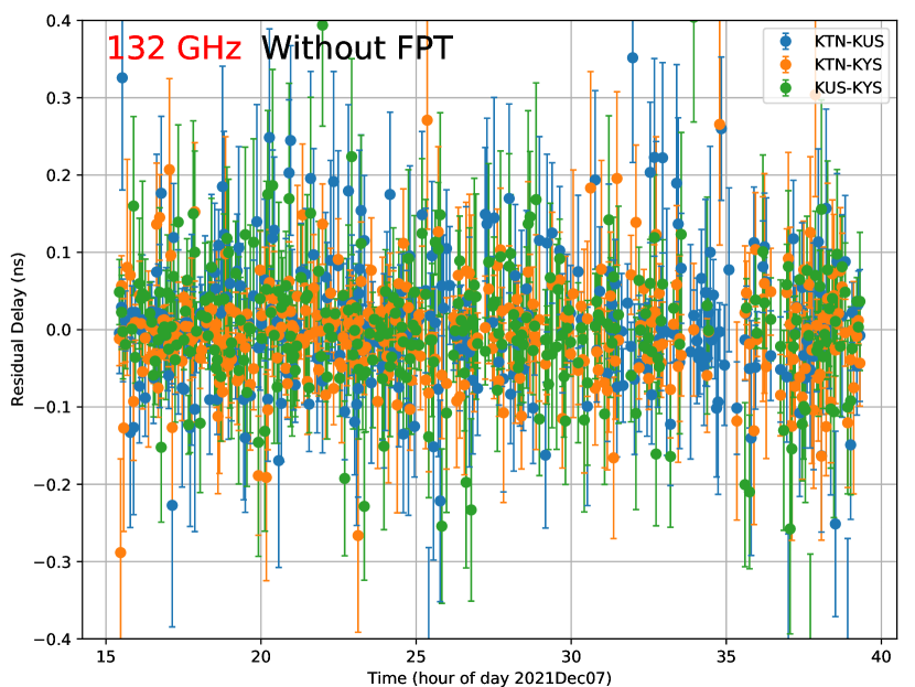
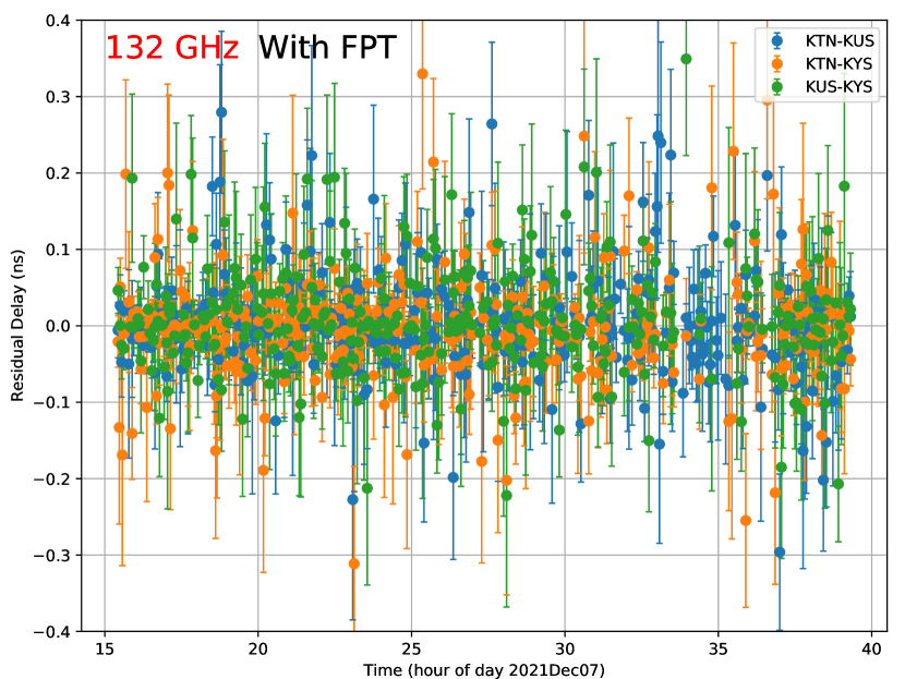
Figure 6: Post-fitting residuals at different bands

Table 4: Geodetic results

Band	Frequency	Atmospheric phase	Recoverable	Used	WRMS	chi2pdof	KTN - KUS	KTN - KYS	KUS - KYS
ID	(MHz)	calibration	delays	delays	(ps)		(mm)	(mm)	(mm)
K	21984	NO	1447 (99.5%)	1444 (99.2%)	12.38	1.00	358342595.57$\pm$0.78	476351705.73$\pm$0.82	304829482.93$\pm$0.71
		$\phi_{Self\_K}$	1447 (99.5%)	1444 (99.2%)	12.31	1.00	358342595.63$\pm$0.78	476351705.73$\pm$0.81	304829482.85$\pm$0.71
Q	42620	NO	484 (99.8%)	483 (99.6%)	11.64	1.00	-	476351705.86$\pm$0.97	-
		$\phi_{FPT\_Q}$	484 (99.8%)	483 (99.6%)	11.76	1.00	-	476351706.24$\pm$0.98	-
W	87936	NO	1371 (94.2%)	1369 (94.1%)	25.02	1.00	358342592.57$\pm$1.65	476351702.87$\pm$1.83	304829480.99$\pm$1.61
		$\phi_{FPT\_W}$	1397 (96.0%)	1389 (95.5%)	20.46	1.00	358342593.85$\pm$1.26	476351703.33$\pm$1.53	304829480.73$\pm$1.37
D	131904	NO	936 (64.3%)	934 (64.2%)	39.34	1.00	358342599.57$\pm$3.60	476351707.85$\pm$3.61	304829482.82$\pm$4.19
		$\phi_{FPT\_D}$	1038 (71.3%)	1032 (70.9%)	27.56	0.99	358342595.64$\pm$2.60	476351705.15$\pm$2.94	304829482.85$\pm$3.00

We performed a comparative analysis of WRMS post-fit delay residuals (pfdr) and estimated baseline lengths, as detailed in Table 4 and Figure 6, considering various frequency bands and the presence or absence of FPT. The baseline lengths estimated and reported in Table 4 are consistent with their respective uncertainties.

The post-fit delay residuals exhibit a WRMS of 12.4 ps at K band and 11.8 ps at Q band. When employing FPT, there is no noticeable difference in WRMS at K and Q bands. This suggests that the impact of atmospheric phase fluctuations at K and Q bands, particularly for baselines of less than 500 km and 2-minute scans, is minimal. This finding aligns with the similar closure group delays observed in Figure 5 and Table 3. Notably, the delay accuracy at the Q band is similar with that at the K band, and the slightly smaller WRMS at the Q band may be attributed to reduced ionospheric effects.

In the case of W and D bands, the visibility phases are significantly affected by atmospheric turbulence. As depicted in Figure 3, FPT enhances fringe SNR, leading to an additional 100 delay observables at the D band. It is worth noting that the W band already boasts a very high detection rate ($\sim 95\%$). Additionally, FPT reduced systematic errors in group delay and delay rate. The WRMS of the post-fitting residuals decreased from 25.0 ps to 20.5 ps at the W band and from 39.3 ps to 27.6 ps at the D band. This indicates that the errors introduced by atmospheric phase fluctuations contributing to the WRMS are $\sim$14 ps for the W band and $\sim$28 ps for the D band in this experiment. This finding aligns with the effects observed in closure group delays in Figure 5 and Table 3. The baseline lengths can be different at 4 mm between without and with FPT. And using FPT, the baseline lengths at W and D bands are generally closer to that of the K band. Therefore, calibration for atmospheric phase fluctuations is necessary in geodetic VLBI at millimeter wavebands.

The source positions estimated in geodetic analysis for this experiment achieve milliarcsecond precision, posing challenges in investigating sub-milliarcsecond frequency-dependent position offsets. Nevertheless, this can be achieved with multiple epochs, extended baselines, and/or including the SFPR method.

5 Conclusion and Outlook

We have successfully conducted the first simultaneous geodetic and astrometric VLBI experiment at 22/43/88/132 GHz with KVN. Our achievement includes a high detection rate of approximately $95\%$ at the W band and about $70\%$ at the D band. Moreover, we have obtained competitive accuracy when compared to traditional centimeter wavebands, with the WRMS of the post-fitting residuals measuring 12.4 ps at K band, 11.8 ps at Q band, 20.5 ps at W band, and 27.6 ps at D band. This experiment demonstrates that the millimeter waveband can be used for geodetic applications with high precision.

For the first time, we introduced the FPT method to geodetic VLBI analysis, an approach for calibrating atmospheric phase fluctuations. Our results demonstrated that FPT improves fringe detection and enhances the accuracy of delay measurements at the W and D bands. We found that atmospheric phase fluctuations, prevalent with baselines under 500 km and 2-minute scans, contribute to errors of approximately 14 ps at the W band and 28 ps at the D band. These fluctuations represent a major error source in millimeter-wave geodetic VLBI and can be effectively mitigated through the FPT method for general sources. It is important to emphasize that FPT proves highly beneficial for geodetic mm-VLBI observations. This extends beyond merely detecting weaker sources, encompassing the precise measurement of frequency-dependent offsets in source positions at millimeter wavebands (Rioja & Dodson, 2011).

The challenges we previously believed regarding geodetic VLBI at the millimeter waveband might be surmountable. The high detection rate at 22/43/88/132 GHz for 82 sources has encouraged us to complete an all-sky distributed source catalog for geodetic VLBI and mm-VLBI studies in astrophysics (e.g., Dodson et al. 2017). The number of detectable ICRF sources at K/Q/W bands is expected to exceed several hundred with KVN (Xu et al., 2024). Typical mm-VLBI observations (above 80 GHz) require reference pointing scans to ensure accurate antenna pointing. In this experiment, such scans were not implemented due to the lack of support in SKED. Nevertheless, the results were satisfactory, owing to the high pointing accuracy of KVN. Further efforts to incorporate reference pointing scans into geodetic mm-VLBI scheduling are currently underway. The precision of group delay with broad bandwidth synthesis from 20 to 100 GHz with KVN can be comparable to or better than VGOS, as demonstrated by a fringe in Xu et al. (2024). The KVN phase-cal system is also being tested to determine the delay and phase offsets among different bands and monitor the effect of changes in ambient temperature on components of the signal chain. While the current KVN baseline is relatively short and limits our ability to explore the ionosphere, source structure, and frequency-dependent offsets in source positions, it’s worth noting that simultaneous tri-band (K/Q/W) receivers are undergoing global development (e.g., Dodson et al. 2023). We anticipate that we will have access to longer baselines in the coming years, enabling more comprehensive investigations in these areas as mentioned in Section 1.

Appendix A Source catalog

The 82 sources used in this experiment are listed in Table 5.

Table 5: 82 sources for geodetic VLBI at K/Q/W/D band

ID	J2000	IVS	Flux density	Flux density	Flux density	Flux density	SNR K	SNR Q	SNR W	SNR D
	Name	Name	K (mJy)	Q (mJy)	W (mJy)	D (mJy)
1	J0006$-$0623	0003$-$066	4498$\pm$348	2750$\pm$99	947$\pm$570	459$\pm$162	827$\pm$161	526$\pm$134	73$\pm$36	11$\pm$11
2	J0019$+$7327	0016$+$731	1794$\pm$152	1543$\pm$62	834$\pm$222	393$\pm$140	357$\pm$75	337$\pm$45	62$\pm$16	17$\pm$9
3	J0102$+$5824	0059$+$581	4330$\pm$374	3970$\pm$270	2530$\pm$1099	795$\pm$747	953$\pm$127	993$\pm$70	245$\pm$45	90$\pm$39
4	J0108$+$0135	0106$+$013	4603$\pm$373	3740$\pm$324	2216$\pm$590	951$\pm$341	822$\pm$200	818$\pm$236	198$\pm$70	53$\pm$29
5	J0116$-$1136	0113$-$118	1635$\pm$133	1207$\pm$64	700$\pm$297	371$\pm$164	304$\pm$54	256$\pm$56	47$\pm$16	13$\pm$7
6	J0121$+$1149	0119$+$115	922$\pm$102	376$\pm$45	305$\pm$206	347$\pm$306	170$\pm$38	80$\pm$30	10$\pm$11	6$\pm$2
7	J0136$+$4751	0133$+$476	2589$\pm$208	2334$\pm$72	1453$\pm$312	748$\pm$273	520$\pm$79	525$\pm$77	123$\pm$30	41$\pm$18
8	J0152$+$2207	0149$+$218	526$\pm$78	465$\pm$3	311$\pm$66	271$\pm$79	105$\pm$10	106$\pm$19	24$\pm$5	7$\pm$2
9	J0228$+$6721	4C67.05	835$\pm$92	705$\pm$39	442$\pm$137	308$\pm$153	162$\pm$52	151$\pm$14	30$\pm$11	10$\pm$5
10	J0237$+$2848	0234$+$285	1752$\pm$129	2113$\pm$5	1838$\pm$343	1050$\pm$313	371$\pm$40	444$\pm$0	136$\pm$12	52$\pm$13
11	J0242$+$1101	0239$+$108	715$\pm$79	642$\pm$11	432$\pm$145	281$\pm$159	144$\pm$28	162$\pm$42	35$\pm$11	9$\pm$5
12	J0259$-$0019	0256$-$005	423$\pm$69	303$\pm$3	215$\pm$74	241$\pm$160	84$\pm$13	68$\pm$8	11$\pm$3	5$\pm$0
13	J0303$+$4716	0300$+$470	1188$\pm$100	905$\pm$35	549$\pm$149	344$\pm$157	233$\pm$31	176$\pm$27	46$\pm$8	16$\pm$5
14	J0325$+$2224	0322$+$222	740$\pm$78	689$\pm$8	452$\pm$147	351$\pm$84	149$\pm$20	156$\pm$11	36$\pm$5	11$\pm$5
15	J0336$+$3218	NRAO140	1348$\pm$140	1563$\pm$76	1225$\pm$257	608$\pm$208	282$\pm$42	361$\pm$45	94$\pm$17	29$\pm$12
16	J0339$-$0146	CTA26	395$\pm$103	432$\pm$28	421$\pm$94	386$\pm$190	70$\pm$22	84$\pm$22	24$\pm$7	7$\pm$3
17	J0422$+$0219	0420$+$022	611$\pm$83	458$\pm$10	312$\pm$149	314$\pm$107	107$\pm$24	90$\pm$25	17$\pm$6	5$\pm$2
18	J0422$+$5324	0418$+$532	283$\pm$77	232$\pm$6	201$\pm$93	245$\pm$84	53$\pm$17	44$\pm$15	9$\pm$3	5$\pm$1
19	J0423$+$4150	0420$+$417	1120$\pm$110	918$\pm$48	536$\pm$140	364$\pm$71	225$\pm$37	166$\pm$44	40$\pm$8	12$\pm$6
20	J0449$+$1121	0446$+$112	829$\pm$93	673$\pm$11	496$\pm$136	299$\pm$178	153$\pm$33	130$\pm$45	30$\pm$11	7$\pm$4
21	J0457$-$2324	0454$-$234	3350$\pm$507	2530$\pm$837	2120$\pm$278	1070$\pm$235	573$\pm$155	504$\pm$168	122$\pm$48	37$\pm$19
22	J0501$-$0159	0458$-$020	2883$\pm$237	2717$\pm$47	1955$\pm$216	904$\pm$227	564$\pm$96	624$\pm$121	153$\pm$38	53$\pm$23
23	J0530$+$1331	0528$+$134	1523$\pm$175	1494$\pm$22	1021$\pm$364	404$\pm$220	308$\pm$61	342$\pm$88	75$\pm$25	23$\pm$13
24	J0533$+$4822	0529$+$483	868$\pm$87	702$\pm$5	453$\pm$158	278$\pm$142	179$\pm$26	157$\pm$23	35$\pm$7	11$\pm$5
25	J0607$-$0834	0605$-$085	2204$\pm$201	1724$\pm$73	972$\pm$250	449$\pm$108	413$\pm$73	361$\pm$74	68$\pm$17	17$\pm$9
26	J0646$+$4451	0642$+$449	1817$\pm$152	1180$\pm$68	600$\pm$158	324$\pm$108	385$\pm$60	254$\pm$57	43$\pm$11	12$\pm$6
27	J0650$-$1637	0648$-$165	2498$\pm$249	2141$\pm$71	1517$\pm$254	861$\pm$174	440$\pm$131	310$\pm$137	76$\pm$39	23$\pm$17
28	J0725$-$0054	0723$-$008	2121$\pm$572	2014$\pm$57	1385$\pm$328	786$\pm$172	291$\pm$147	307$\pm$135	73$\pm$38	19$\pm$19
29	J0730$-$1141	0727$-$115	2619$\pm$180	1874$\pm$7	1210$\pm$200	656$\pm$171	494$\pm$62	383$\pm$33	90$\pm$8	31$\pm$8
30	J0738$+$1742	0735$+$178	867$\pm$93	867$\pm$3	788$\pm$274	495$\pm$132	167$\pm$34	183$\pm$46	56$\pm$17	21$\pm$11
31	J0808$-$0751	0805$-$077	2496$\pm$222	2680$\pm$59	2395$\pm$461	1556$\pm$564	240$\pm$39	253$\pm$40	60$\pm$10	19$\pm$8
32	J0808$+$4052	0805$+$410	1159$\pm$107	1019$\pm$19	709$\pm$239	392$\pm$135	387$\pm$80	381$\pm$89	107$\pm$35	30$\pm$22
33	J0811$+$0146	0808$+$019	696$\pm$83	744$\pm$7	680$\pm$216	447$\pm$103	127$\pm$23	137$\pm$26	39$\pm$10	14$\pm$7
34	J0836$-$2016	0834$-$201	398$\pm$78	239$\pm$6	250$\pm$127	310$\pm$162	68$\pm$15	38$\pm$9	8$\pm$2	5$\pm$0
35	J0854$+$2006	OJ287	8535$\pm$694	8121$\pm$129	5995$\pm$253	3129$\pm$392	1604$\pm$303	1604$\pm$386	414$\pm$105	151$\pm$69
36	J0909$+$0121	0906$+$015	1090$\pm$103	961$\pm$3	696$\pm$121	475$\pm$203	194$\pm$31	174$\pm$29	41$\pm$8	13$\pm$6
37	J0921$+$6215	0917$+$624	920$\pm$100	830$\pm$52	516$\pm$130	355$\pm$103	191$\pm$29	188$\pm$32	45$\pm$11	17$\pm$7
38	J0927$+$3902	4C39.25	6298$\pm$544	3338$\pm$1227	1750$\pm$239	780$\pm$167	952$\pm$140	685$\pm$129	115$\pm$14	36$\pm$8
39	J0948$+$4039	0945$+$408	647$\pm$94	505$\pm$29	311$\pm$49	261$\pm$60	95$\pm$19	89$\pm$12	16$\pm$4	5$\pm$2
40	J0956$+$2515	OK290	940$\pm$89	840$\pm$7	565$\pm$69	349$\pm$114	191$\pm$28	186$\pm$23	46$\pm$7	16$\pm$3
41	J0958$+$4725	0955$+$476	984$\pm$96	860$\pm$27	605$\pm$102	404$\pm$115	201$\pm$35	192$\pm$36	49$\pm$11	18$\pm$8
42	J1043$+$2408	1040$+$244	908$\pm$89	703$\pm$13	483$\pm$77	333$\pm$121	180$\pm$26	152$\pm$10	36$\pm$4	12$\pm$3
43	J1048$-$1909	1045$-$188	1068$\pm$93	896$\pm$15	646$\pm$42	421$\pm$59	198$\pm$23	175$\pm$17	45$\pm$6	16$\pm$4
44	J1058$+$0133	1055$+$018	5941$\pm$431	5160$\pm$115	3839$\pm$413	2201$\pm$507	1122$\pm$185	970$\pm$224	270$\pm$56	89$\pm$40
45	J1058$+$8114	1053$+$815	238$\pm$63	288$\pm$10	304$\pm$79	270$\pm$84	44$\pm$7	55$\pm$7	17$\pm$5	5$\pm$3
46	J1146$+$3958	1144$+$402	1355$\pm$105	964$\pm$115	598$\pm$106	356$\pm$85	285$\pm$42	247$\pm$31	50$\pm$9	19$\pm$6
47	J1147$-$0724	1145$-$071	642$\pm$92	375$\pm$73	218$\pm$100	278$\pm$170	117$\pm$21	68$\pm$24	8$\pm$3	5$\pm$0
48	J1159$+$2914	1156$+$295	5792$\pm$451	5931$\pm$213	5906$\pm$805	2916$\pm$359	1156$\pm$174	1276$\pm$156	365$\pm$71	149$\pm$50
49	J1215$-$1731	1213$-$172	2384$\pm$277	2095$\pm$72	1372$\pm$264	697$\pm$191	432$\pm$120	386$\pm$128	86$\pm$37	22$\pm$16
50	J1230$+$1223	3C274	1644$\pm$169	1281$\pm$123	1055$\pm$250	673$\pm$177	318$\pm$46	300$\pm$50	85$\pm$15	32$\pm$14
51	J1256$-$0547	3C279	24891$\pm$1725	22193$\pm$824	15208$\pm$1651	7325$\pm$1443	4492$\pm$715	4254$\pm$800	1120$\pm$268	356$\pm$118
52	J1310$+$3220	1308$+$326	2444$\pm$194	2420$\pm$86	1725$\pm$234	889$\pm$220	519$\pm$78	612$\pm$74	149$\pm$19	46$\pm$13
53	J1337$-$1257	1334$-$127	2662$\pm$207	2056$\pm$594	1967$\pm$250	1046$\pm$236	472$\pm$121	449$\pm$156	114$\pm$56	36$\pm$28
54	J1357$+$1919	1354$+$195	1741$\pm$141	1648$\pm$128	1018$\pm$248	480$\pm$177	357$\pm$48	422$\pm$50	87$\pm$17	25$\pm$13
55	J1419$+$5423	1418$+$546	622$\pm$98	538$\pm$54	355$\pm$80	271$\pm$152	130$\pm$25	114$\pm$24	27$\pm$8	8$\pm$4
56	J1459$+$7140	3C309.1	335$\pm$107	279$\pm$32	197$\pm$53	269$\pm$104	62$\pm$22	50$\pm$6	7$\pm$2	5$\pm$0
57	J1504$+$1029	1502$+$106	831$\pm$86	721$\pm$21	450$\pm$102	305$\pm$108	182$\pm$24	182$\pm$10	41$\pm$6	16$\pm$4
58	J1512$-$0905	1510$-$089	3643$\pm$245	2669$\pm$340	1656$\pm$260	771$\pm$195	694$\pm$115	593$\pm$113	126$\pm$32	40$\pm$15
59	J1540$+$1447	1538$+$149	974$\pm$97	901$\pm$4	753$\pm$63	546$\pm$141	163$\pm$19	153$\pm$0	42$\pm$5	13$\pm$5
60	J1549$+$0237	1546$+$027	2464$\pm$162	1568$\pm$59	693$\pm$295	275$\pm$177	478$\pm$99	395$\pm$91	47$\pm$24	8$\pm$7
61	J1613$+$3412	1611$+$343	2125$\pm$191	1228$\pm$63	539$\pm$271	362$\pm$110	436$\pm$53	240$\pm$13	37$\pm$14	13$\pm$4
62	J1625$-$2527	1622$-$253	1014$\pm$103	756$\pm$18	489$\pm$58	439$\pm$141	169$\pm$24	126$\pm$18	26$\pm$4	6$\pm$1
63	J1638$+$5720	1637$+$574	926$\pm$85	987$\pm$66	765$\pm$187	463$\pm$142	202$\pm$24	219$\pm$12	65$\pm$12	26$\pm$9
64	J1642$-$0621	1639$-$062	1374$\pm$123	1104$\pm$42	696$\pm$112	371$\pm$152	268$\pm$48	240$\pm$49	52$\pm$11	15$\pm$6
65	J1658$+$0741	1655$+$077	1342$\pm$107	1167$\pm$41	741$\pm$157	385$\pm$85	280$\pm$41	290$\pm$31	64$\pm$10	22$\pm$7
66	J1733$-$1304	NRAO530	3360$\pm$123	1789$\pm$59	1076$\pm$136	493$\pm$89	612$\pm$95	334$\pm$73	76$\pm$16	17$\pm$5
67	J1734$+$3857	1732$+$389	1221$\pm$106	1229$\pm$61	843$\pm$278	480$\pm$213	262$\pm$35	291$\pm$30	70$\pm$8	25$\pm$8
68	J1751$+$0939	1749$+$096	2768$\pm$199	2505$\pm$81	1633$\pm$208	826$\pm$193	616$\pm$80	653$\pm$46	152$\pm$20	51$\pm$12
69	J1753$+$2848	1751$+$288	2235$\pm$173	1736$\pm$60	1002$\pm$230	451$\pm$206	430$\pm$65	378$\pm$57	76$\pm$12	27$\pm$6
70	J1800$+$7828	1803$+$784	2099$\pm$179	1739$\pm$113	1073$\pm$212	579$\pm$152	405$\pm$63	337$\pm$44	83$\pm$17	27$\pm$12
71	J1824$+$5651	1823$+$568	926$\pm$164	787$\pm$63	513$\pm$129	355$\pm$96	199$\pm$39	179$\pm$25	41$\pm$13	14$\pm$7
72	J1849$+$6705	1849$+$670	1604$\pm$282	1257$\pm$267	616$\pm$319	377$\pm$153	306$\pm$121	268$\pm$91	56$\pm$22	16$\pm$9
73	J1911$-$2006	1908$-$201	2374$\pm$231	1769$\pm$206	1136$\pm$163	563$\pm$132	393$\pm$107	282$\pm$114	68$\pm$31	18$\pm$9
74	J2000$-$1748	1958$-$179	1803$\pm$163	1783$\pm$97	1232$\pm$203	612$\pm$179	309$\pm$54	332$\pm$57	86$\pm$25	22$\pm$12
75	J2115$+$2933	2113$+$293	849$\pm$75	626$\pm$8	369$\pm$173	253$\pm$109	168$\pm$26	139$\pm$23	27$\pm$5	6$\pm$3
76	J2134$-$0153	2131$-$021	1484$\pm$166	1088$\pm$149	642$\pm$227	386$\pm$164	285$\pm$63	219$\pm$79	45$\pm$18	9$\pm$9
77	J2139$+$1423	2136$+$141	1434$\pm$118	811$\pm$42	347$\pm$99	249$\pm$137	234$\pm$61	152$\pm$43	22$\pm$7	5$\pm$1
78	J2152$+$1734	2150$+$173	300$\pm$70	249$\pm$8	246$\pm$103	238$\pm$288	41$\pm$9	41$\pm$10	9$\pm$3	5$\pm$0
79	J2229$-$0832	2227$-$088	2460$\pm$186	2570$\pm$132	1542$\pm$577	537$\pm$337	471$\pm$76	547$\pm$96	119$\pm$33	32$\pm$20
80	J2232$+$1143	CTA102	3792$\pm$285	3733$\pm$1679	3140$\pm$619	755$\pm$498	749$\pm$135	1061$\pm$256	283$\pm$97	73$\pm$61
81	J2236$+$2828	2234$+$282	1940$\pm$144	1870$\pm$100	1152$\pm$762	664$\pm$159	388$\pm$64	413$\pm$77	94$\pm$25	27$\pm$16
82	J2327$+$0940	2325$+$093	1328$\pm$123	1371$\pm$95	792$\pm$438	505$\pm$121	262$\pm$51	312$\pm$72	59$\pm$20	16$\pm$11

Note. — The flux density values are obtained from KVN baseline ($<500$ km) amplitude using AIPS, while the SNR with 2-min scans is produced by fourfit. These values (weighted averages and standard deviations) are provided as a reference for conducting observations and may not be accurate for AGN astrophysics studies. The different standard deviations observed in the baseline amplitudes and SNRs may be attributed to variations in weather conditions, elevation angles, and pointing accuracy.

References

- Akiyama et al. (2022) Akiyama, K., Algaba, J.-C., An, T., et al. 2022, Galaxies, 10, 113, doi: 10.3390/galaxies10060113
- Anderson & Xu (2018) Anderson, J. M., & Xu, M. H. 2018, Journal of Geophysical Research (Solid Earth), 123, 10,162, doi: 10.1029/2018JB015550
- Astropy Collaboration et al. (2013) Astropy Collaboration, Robitaille, T. P., Tollerud, E. J., et al. 2013, A&A, 558, A33, doi: 10.1051/0004-6361/201322068
- Blackburn et al. (2019) Blackburn, L., Chan, C.-k., Crew, G. B., et al. 2019, ApJ, 882, 23, doi: 10.3847/1538-4357/ab328d
- Blandford & Königl (1979) Blandford, R. D., & Königl, A. 1979, ApJ, 232, 34, doi: 10.1086/157262
- Bohm & Schuh (2013) Bohm, J., & Schuh, H. 2013, Atmospheric Effects in Space Geodesy, doi: 10.1007/978-3-642-36932-2
- Bolotin et al. (2023) Bolotin, S., Baver, K., Bérubé, M., & Gipson, J. 2023, in International VLBI Service for Geodesy and Astrometry 2022 General Meeting Proceedings, ed. K. L. Armstrong, D. Behrend, & K. D. Baver, 159–163
- Bolotin et al. (2014) Bolotin, S., Baver, K., Gipson, J., Gordon, D., & MacMillan, D. 2014, in International VLBI Service for Geodesy and Astrometry 2014 General Meeting Proceedings: ”VGOS: The New VLBI Network, 253–257
- Bolotin et al. (2016) Bolotin, S., Baver, K., Gipson, J., Gordon, D., & MacMillan, D. 2016, in New Horizons with VGOS, ed. D. Behrend, K. D. Baver, & K. L. Armstrong, 222–224
- Charlot (2022) Charlot, P. 2022, in IAU General Assembly. https://www.iau.org/static/science/scientific_bodies/divisions/a/2022/Div-A-3_9-1_Patrick_Charlot.pdf
- Charlot et al. (2020) Charlot, P., Jacobs, C. S., Gordon, D., et al. 2020, A&A, 644, A159, doi: 10.1051/0004-6361/202038368
- Davis et al. (1985) Davis, J. L., Herring, T. A., Shapiro, I. I., Rogers, A. E. E., & Elgered, G. 1985, Radio Science, 20, 1593, doi: 10.1029/RS020i006p01593
- de Witt et al. (2023) de Witt, A., Jacobs, C. S., Gordon, D., et al. 2023, AJ, 165, 139, doi: 10.3847/1538-3881/aca012
- Deller et al. (2011) Deller, A. T., Brisken, W. F., Phillips, C. J., et al. 2011, PASP, 123, 275, doi: 10.1086/658907
- Dodson et al. (2017) Dodson, R., Rioja, M. J., Jung, T., et al. 2017, New A Rev., 79, 85, doi: 10.1016/j.newar.2017.09.003
- Dodson et al. (2023) Dodson, R., García-Miró, C., Giroletti, M., et al. 2023, arXiv e-prints, arXiv:2306.04516, doi: 10.48550/arXiv.2306.04516
- Fish (2015) Fish, V. 2015, in Mm-VLBI Data Processing Workshop. https://www.jive.eu/mm-vlbi2015/Documents/Fish_tutorial.pdf
- Fomalont et al. (2009) Fomalont, E., Kopeikin, S., Lanyi, G., & Benson, J. 2009, ApJ, 699, 1395, doi: 10.1088/0004-637X/699/2/1395
- Gaia Collaboration et al. (2022) Gaia Collaboration, Klioner, S. A., Lindegren, L., et al. 2022, A&A, 667, A148, doi: 10.1051/0004-6361/202243483
- Gipson (2018) Gipson, J. 2018, SKED VLBI Scheduling Software. Goddard Space FLight Center
- Greisen (2003) Greisen, E. W. 2003, in Astrophysics and Space Science Library, Vol. 285, Information Handling in Astronomy - Historical Vistas, ed. A. Heck, 109, doi: 10.1007/0-306-48080-8_7
- Hada et al. (2011) Hada, K., Doi, A., Kino, M., et al. 2011, Nature, 477, 185, doi: 10.1038/nature10387
- Han et al. (2013) Han, S.-T., Lee, J.-W., Kang, J., et al. 2013, PASP, 125, 539, doi: 10.1086/671125
- Hoak et al. (2022) Hoak, D., Barrett, J., Crew, G., & Pfeiffer, V. 2022, Galaxies, 10, 119, doi: 10.3390/galaxies10060119
- Hunter (2007) Hunter, J. D. 2007, Computing in Science & Engineering, 9, 90, doi: 10.1109/MCSE.2007.55
- Jeong et al. (2022) Jeong, S.-H., Lee, W. K., Jang, S., et al. 2022, Space Weather, 20, e2022SW003131, doi: https://doi.org/10.1029/2022SW003131
- Jung (2018) Jung, T. 2018, in 14th European VLBI Network Symposium & Users Meeting (EVN 2018), 104
- Jung et al. (2011) Jung, T., Sohn, B. W., Kobayashi, H., et al. 2011, PASJ, 63, 375, doi: 10.1093/pasj/63.2.375
- Jung et al. (2015) Jung, T., Dodson, R., Han, S.-T., et al. 2015, Journal of Korean Astronomical Society, 48, 277, doi: 10.5303/JKAS.2015.48.5.277
- Kettenis et al. (2006) Kettenis, M., van Langevelde, H. J., Reynolds, C., & Cotton, B. 2006, in Astronomical Society of the Pacific Conference Series, Vol. 351, Astronomical Data Analysis Software and Systems XV, ed. C. Gabriel, C. Arviset, D. Ponz, & S. Enrique, 497
- Koryukova et al. (2022) Koryukova, T. A., Pushkarev, A. B., Plavin, A. V., & Kovalev, Y. Y. 2022, MNRAS, 515, 1736, doi: 10.1093/mnras/stac189810.48550/arXiv.2201.04359
- Lanyi et al. (2010) Lanyi, G. E., Boboltz, D. A., Charlot, P., et al. 2010, AJ, 139, 1695, doi: 10.1088/0004-6256/139/5/1695
- Lee et al. (2017) Lee, J. A., Sohn, B. W., Jung, T., Byun, D.-Y., & Lee, J. W. 2017, ApJS, 228, 22, doi: 10.3847/1538-4365/228/2/22
- Lee et al. (2014) Lee, S.-S., Petrov, L., Byun, D.-Y., et al. 2014, AJ, 147, 77, doi: 10.1088/0004-6256/147/4/77
- MacMillan (1995) MacMillan, D. S. 1995, Geophys. Res. Lett., 22, 1041, doi: 10.1029/95GL00887
- Niell et al. (2018) Niell, A., Barrett, J., Burns, A., et al. 2018, Radio Science, 53, 1269, doi: 10.1029/2018RS006617
- Niell et al. (2021) Niell, A. E., Barrett, J. P., Cappallo, R. J., et al. 2021, Journal of Geodesy, 95, 65, doi: 10.1007/s00190-021-01505-9
- Nothnagel (2019) Nothnagel, A. 2019, Very Long Baseline Interferometry, ed. W. Freeden & R. Rummel (Berlin, Heidelberg: Springer Berlin Heidelberg), 1–58, doi: 10.1007/978-3-662-46900-2_110-1
- Petrov (2024) Petrov, L. 2024, arXiv e-prints, arXiv:2404.08800, doi: 10.48550/arXiv.2404.08800
- Rioja & Dodson (2011) Rioja, M., & Dodson, R. 2011, AJ, 141, 114, doi: 10.1088/0004-6256/141/4/114
- Rioja & Dodson (2020) Rioja, M. J., & Dodson, R. 2020, A&ARv, 28, 6, doi: 10.1007/s00159-020-00126-z
- Rioja et al. (2015) Rioja, M. J., Dodson, R., Jung, T., & Sohn, B. W. 2015, AJ, 150, 202, doi: 10.1088/0004-6256/150/6/202
- Saastamoinen (1972) Saastamoinen, J. 1972, in The Use of Artificial Satellites for Geodesy, Vol. 15, 247, doi: 10.1029/GM015p0247
- Sovers et al. (1998) Sovers, O. J., Fanselow, J. L., & Jacobs, C. S. 1998, Reviews of Modern Physics, 70, 1393, doi: 10.1103/RevModPhys.70.1393
- Walker (2022) Walker, R. 2022, The sched user manual
- Whitney et al. (2022) Whitney, A. R., Cappallo, R., Aldrich, W., et al. 2022, HOPS: Haystack Observatory Postprocessing System, Astrophysics Source Code Library, record ascl:2205.019. http://ascl.net/2205.019
- Xu et al. (2021a) Xu, M. H., Anderson, J. M., Heinkelmann, R., et al. 2021a, Journal of Geodesy, 95, 51, doi: 10.1007/s00190-021-01496-7
- Xu et al. (2016) Xu, M. H., Heinkelmann, R., Anderson, J. M., et al. 2016, AJ, 152, 151, doi: 10.3847/0004-6256/152/5/151
- Xu et al. (2022) Xu, M. H., Savolainen, T., Anderson, J. M., et al. 2022, A&A, 663, A83, doi: 10.1051/0004-6361/202140840
- Xu et al. (2024) Xu, S., Jung, T., & Byun, D.-Y. 2024, Geodetic and Astrometric VLBI at K/Q/W/D Bands with the KVN, Zenodo, doi: 10.5281/zenodo.10902979
- Xu et al. (2021b) Xu, S., Jike, T., Jung, T., et al. 2021b, in 25th European VLBI Group for Geodesy and Astrometry Working Meeting, ed. R. Haas, Vol. 25, 71–73