Active Brownian particle under stochastic position and orientation resetting in a harmonic trap

Abstract

We present an exact analytical study of an Active Brownian Particle (ABP) subject to both position and orientation stochastic resetting in a two-dimensional harmonic trap. Utilizing a Fokker-Planck-based renewal approach, we derive the system’s exact moments, including the mean parallel displacement, mean squared displacement (MSD), and the fourth-order moment of displacement, and compare these with numerical simulations. To capture deviations from Gaussian behavior, we analyze the excess kurtosis, which reveals rich dynamical crossovers over time. These transitions span from Gaussian behavior (zero excess kurtosis) to two distinct non-Gaussian regimes: an activity-dominated regime (negative excess kurtosis) and a resetting-dominated regime (positive excess kurtosis). Furthermore, we quantify the steady-state phase diagrams by varying three key control parameters: activity, resetting rate, and harmonic trap strength, using steady-state excess kurtosis as the primary metric.

Keywords: active Brownian particle, stochastic resetting, harmonic trap, exact moments, excess kurtosis, phase diagrams

1 Introduction

Active particles convert energy into motility and exhibit a wide range of dynamical behaviors [1, 2, 3, 4, 5, 6]. These behaviors are observed across diverse systems, including cytoskeletal filaments in motor protein assays [7, 8, 9, 10], bird flocks [11], fish schools [12], and artificial systems like active colloids and robots. Active particles are inherently out of equilibrium, displaying collective phenomena such as flocking [13, 14, 15], clustering [16, 17, 18], and phase separation [19, 20]. Even at the single-particle level, they exhibit diverse dynamical behaviors, including short-time ballistic motion [21, 22, 23, 24, 25, 26], nonequilibrium steady states in confinement [27, 28, 29, 30], and dynamical transitions in relaxation and first passage properties [31, 32, 33, 34]. Recent studies have demonstrated enhanced control over active agents for decision-making by space dependent rotational diffusion coefficient [35], as well as using external or internal cues, such as magnetic fields [36], chemical gradients [37], and acoustic waves [38, 39], to control their speed and orientation.

Stochastic resetting is a protocol that resets a dynamical system to a specific state, primarily governing the nonequilibrium steady state (NESS) through a continuous influx of probability from resetting. This process can lead to dynamical transitions during the system’s relaxation to the NESS and often results in a non-monotonic mean first passage time [40, 41, 42, 43, 44]. The resetting strategy has broad applications across various systems, including population dynamics and biological processes, particularly in optimizing search problems [45, 46, 47, 48, 49, 50, 51, 52]. The impact of resetting on different diffusive dynamics has also been extensively studied [53, 54, 55, 56, 57, 58, 59, 60, 61, 62, 63, 64, 60]. Resetting has proven to be an optimal navigation strategy for target search, particularly in Brownian motion [40] and under external potentials [65].

The resetting of a free active Brownian agent has been studied recently in [66, 67], with extensions to external confining and absorbing potentials in [68, 69, 70]. Activity introduces new dynamical behavior due to the competition between the internal active timescale and the resetting timescale, first studied in [71]. The first passage properties of active Brownian particle (ABP) and run-and-tumble particle (RTP) under various resetting mechanisms have been explored in [72, 73]. The dynamics of an ABP under position stochastic resetting, orientation stochastic resetting, and combined position and orientation stochastic resetting, focusing on marginal probability distributions, were examined in Kumar et al. [66]. The dynamics under orientation stochastic resetting, using the intermediate scattering function, were studied in [74]. However, the exact dynamics of an ABP under both position and orientation resetting in a harmonic trap, along with an analysis of the steady-state properties, remain unexplored. From the lens of active matter, it is crucial to delve into the intricate interplay between stochastic resetting and activity under the influence of an external force.

In this work, we investigate the exact dynamics of active Brownian particle (ABP) under complete stochastic resetting, involving both position and orientation, in a harmonic trap. We apply the method for exact moment calculations of stiff chains, as described by Hermans et al.[75], to compute the exact moments for the active dynamics case. Using a Fokker-Planck-based approach, we derive the dynamical moment generating equation, which we then use to calculate all dynamical moments. This method has been previously applied to study ABP in a harmonic trap [30], with anisotropic translational noise [76], fluctuating speed [25], and chirality/torque [77], and has also been extended to inertial ABP [26, 78]. Here, we focus on exact moment calculations of ABP under complete stochastic resetting in a harmonic trap using a renewal equation following the Fokker-Planck-based moments calculation. We also characterize the steady-state behavior across various limits and parameter ranges using excess kurtosis.

The remainder of this paper is organized as follows. In Section 2, we introduce the model of an ABP under complete stochastic resetting in a harmonic trap. Using a Fokker-Planck-based approach, we derive the dynamical moment generating equation and apply the final renewal approach to calculate moments under stochastic resetting. This equation is then used to compute the orientation autocorrelation and mean displacement in Section 3. In Section 4, we determine the mean squared displacement and displacement fluctuation. To examine deviations from Gaussian behavior over time, we calculate the fourth-order moment of displacement and the excess kurtosis in Section 5, and characterize the interplay of activity with resetting and trapping in the steady-state phase diagram in Section 6. Finally, we summarize the key results in Section 7.

2 Model and moments generator equation

The standard active Brownian particle in two dimension is described by its position $\mathbf{r}=(x,y)$, and its orientation unit vector ${\bf\hat{u}}=(u_{x},u_{y})$ where $u_{x}=\cos(\theta)$ and $u_{y}=\sin(\theta)$, evolving over time $t$ from their initial values $({\bf r}_{0},{\bf\hat{u}}_{0})$. Stochastic resetting imposed on both ${\bf r}$ and ${\bf\hat{u}}$ intermittently resets to initial values $({\bf r}_{0},{\bf\hat{u}}_{0})$ with rate $r$. The position ${\bf r}$ and orientation ${\bf\hat{u}}$ evolves

$$\dot{\bf r}=v_{0}{\bf\hat{u}}+\sqrt{2D}\bm{\chi}(t)-\mu k{\bf r}\,,$$ (1)

$$\dot{\bf\hat{u}}=\sqrt{2D_{r}}\eta(t){\bf\hat{u}}^{\perp}\,,$$ (2)

$$({\bf r},{\bf\hat{u}})\rightarrow({\bf r}_{0},{\bf\hat{u}}_{0})\,.$$ (3)

Here, $v_{0}$ is the active speed, $D$ is the translation diffusion coefficient, $\mu$ is the mobility, and $k$ is the strength of the harmonic trap. $D_{r}$ is the orientation diffusion coefficient. The noise terms $\bm{\chi}(t)$ and $\eta(t)$ are modeled as Gaussian white noise with zero mean and variances given by $\langle\chi_{i}(t)\chi_{j}(t^{\prime})\rangle=\delta_{ij}\delta(t-t^{\prime})$ and $\langle\eta(t)\eta(t^{\prime})\rangle=\delta(t-t^{\prime})$, respectively. The interplay of the three timescales $D_{r}^{-1}$, $r^{-1}$, and $(\mu k)^{-1}$ would lead to rich behavior for ABP under resetting in a harmonic trap.

We rescale the dynamics using timescale $\tau=D_{r}^{-1}$ and length scale $\ell=\sqrt{D/D_{r}}$. The dynamics (${\bf r}\to{\bf r}/\ell$, ${\bf\hat{u}}\to{\bf\hat{u}}$, $t\to t/\tau$) is now controlled by activity strength defined by Péclet $\mathrm{Pe}=v_{0}\tau/\ell$, resetting rate $r=r\tau$, and trapping strength $\beta=\mu k\ell$. We investigate the dynamics and steady state behavior with varying three dimensionless parameters activity $\mathrm{Pe}$, resetting rate $r$, and trap strength $\beta$.

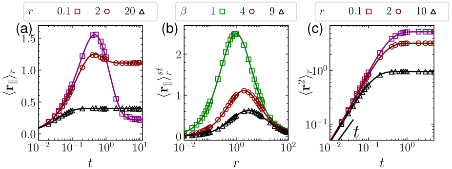
Figure 1: First and second order moments. (a) Mean parallel displacement along initial orientation direction in two dimension (equation (8)) for $r=0.1(\mathrm{square},\Box),~{}2(\mathrm{circle},\circ),~{}10(\mathrm{triangle},\triangle)$ with $\beta=4$ and $\mathrm{Pe}=10$. (b) Steady state displacement along initial orientation $\langle{\bf r}_{\parallel}\rangle^{st}_{r}$ (equation (9)) as a function of resetting rate $r$ for $\beta=1(\mathrm{square},\Box),4(\mathrm{circle},\circ),9(\mathrm{triangle},\triangle)$ with $\mathrm{Pe}=10$. (c) Mean squared displacement (MSD) as function of time (equation (12)) correspond to the parameters in (a). The points represent the simulation results, while the lines correspond to the analytical solutions. The initial position is at the origin with the initial orientation along the $x$-axis.

Moments generator equation

The probability distribution $P({\bf r},{\bf\hat{u}},t)$ of the position ${\bf r}$ and the active orientation ${\bf\hat{u}}$ of the particle follows the Fokker-Planck equation [30]

$$\partial_{t}P({\bf r},{\bf\hat{u}},t) = \nabla^{2}P+\nabla_{\bf\hat{u}}^{2}P-\mathrm{Pe}\,{\bf\hat{u}}\cdot\nabla P-\beta{\bf r}\cdot\nabla P+2\beta P\,,$$ (4)

where $\nabla$ is the two-dimensional Laplacian operator, and $\nabla_{\bf\hat{u}}$ is the Laplacian in the orientation space.

Utilizing the Laplace transform $\tilde{P}({\bf r},{\bf\hat{u}},s)=\int_{0}^{\infty}dt\,e^{-st}\,P({\bf r},{\bf\hat{u}},t)$ and defining the mean of an observable $\langle\psi\rangle_{s}=\int d{\bf r}\,d{\bf\hat{u}}\,\psi({\bf r},{\bf\hat{u}})\tilde{P}({\bf r},{\bf\hat{u}},s)$, multiplying by $\psi({\bf r},{\bf\hat{u}})$ and integrating over all possible $({\bf r},{\bf\hat{u}})$ we find [30],

$$-\langle\psi\rangle_{0}+s\langle\psi\rangle_{s} = \langle\nabla^{2}\psi\rangle_{s}+\langle\nabla_{\bf\hat{u}}^{2}\psi\rangle_{s}+\mathrm{Pe}\langle\,{\bf\hat{u}}\cdot\nabla\psi\rangle_{s}-\beta\langle{\bf r}\cdot\nabla\psi\rangle_{s}\,,$$ (5)

where the initial condition sets $\langle\psi\rangle_{0}=\int d{\bf r}\,d{\bf\hat{u}}\,\psi({\bf r},{\bf\hat{u}})P({\bf r},{\bf\hat{u}},0)$. Without any loss of generality, we consider the initial condition to follow $P({\bf r},{\bf\hat{u}},0)=\delta({\bf r}-{\bf r}_{0})\delta({\bf\hat{u}}-{\bf\hat{u}}_{0})$, where ${\bf r}_{0}$ and ${\bf\hat{u}}_{0}$ are the initial position and orientation respectively. We use equation (5) to calculate exact moments as a function of time without resetting, which is already explored in Chaudhuri et al. [30].

The moments of an ABP under stochastic position and orientation resetting in presence of a harmonic trap can be calculated exactly as [66]

$$\langle\psi(t)\rangle_{r} = e^{-rt}\langle\psi(t)\rangle+r\int_{0}^{t}dt^{\prime}e^{-rt^{\prime}}\langle\psi(t^{\prime})\rangle\,.$$ (6)

We utilize equation (6) to compute the analytic moments exactly under resetting. For comparison with simulations, we perform Euler-Maruyama integration of equations (1) and (2) with stochastic resetting equation (3). The initial position of the particles set at the origin $(x,y)=(0,0)$ which corresponds to the minimum of the harmonic potential, with the orientation along the $x$-axis i.e., $\theta=0$. The positions and orientations of particle stochastically reset to their initial state $(x,y,\theta)=(0,0,0)$ at rate $r$.

3 Mean orientation and mean displacement

We consider the initial orientation of ABP along $\langle{\bf\hat{u}}\rangle={\bf\hat{u}}_{0}$ and proceed to calculate mean orientation. To calculate $\langle{\bf\hat{u}}\rangle$, we use $\psi={\bf\hat{u}}$ in the equation (5), leads to $\langle{\bf\hat{u}}\rangle_{s}={\bf\hat{u}}_{0}/(1+s)$. Inverse Laplace transform leads to the average orientation without stochastic resetting $\langle{\bf\hat{u}}(t)\rangle=e^{-t}{\bf\hat{u}}_{0}$. In the presence of stochastic resetting using renewal approach in equation (6) and taking the dot product with the initial orientation, we get the orientation autocorrelation,

$$\langle{\bf\hat{u}}(t)\cdot{\bf\hat{u}}(0)\rangle_{r} = \frac{r+e^{-(1+r)t}}{(1+r)}\,.$$ (7)

The plot of equation (7) is compared with simulations, as shown in A, figure 5(a). As ($t\to\infty$), the orientation autocorrelation saturates to $r/(1+r)$. In the steady state $\langle{\bf\hat{u}}(t)\cdot{\bf\hat{u}}(0)\rangle_{r}$ varies from $0$ as $r\to 0$ to $1$ as $r\to\infty$.

Now, we proceed to calculate $\langle{\bf r}\rangle_{s}$ we consider the initial position at $\langle{\bf r}\rangle_{0}=0$, using the equation (5) leads to $\langle{\bf r}\rangle_{s}=\mathrm{Pe}\langle{\bf\hat{u}}\rangle_{s}/(s+\beta)$. Substituting $\langle{\bf\hat{u}}\rangle_{s}$ and then inverse Laplace transform gives the mean displacement in the absence of resetting $\langle{\bf r}(t)\rangle$ [30]. The parallel and perpendicular component of the displacement vector to the initial orientation defined as ${\bf\hat{u}}_{0}$ as ${\bf r}_{\parallel}=({\bf r}\cdot{\bf\hat{u}}_{0}){\bf\hat{u}}_{0}$ and ${\bf r}_{\perp}={\bf r}-{\bf r}_{\parallel}$. In the presence of stochastic resetting using renewal approach in equation (6), we get

$$\langle{\bf r}_{\parallel}(t)\rangle_{r}=\frac{\mathrm{Pe}{\bf\hat{u}}_{0}(e^{-(\beta+r)t}-e^{-(1+r)t})}{1-\beta}-\frac{r\mathrm{Pe}{\bf\hat{u}}_{0}}{1-\beta}\left[\frac{1-e^{-(1+r)t}}{1+r}-\frac{1-e^{-(\beta+r)t}}{\beta+r}\right]\,.$$ (8)

In the absence of harmonic trap ($\beta=0$), equation (8) simplifies to ABP under stochastic resetting [66], see A, figure 5(b). In figure 1(a), we plot equation (8) as solid lines, showing excellent agreement with the simulation results represented by the points. For a small resetting rate ($r$), $\langle{\bf r}_{\parallel}(t)\rangle_{r}$ exhibits non-monotonic behavior: it starts with a small value in the short-time, thermally dominated diffusion regime, reaches a maximum at intermediate times in the activity-dominated regime, and then decays back to smaller values due to trapping, see squares ($\Box$) for $r=0.1$ in figure 1(a). At long times, $\langle{\bf r}_{\parallel}(t)\rangle_{r}$ decays to zero in the absence of stochastic resetting [30], exhibiting the same behavior as for low resetting rates. For intermediate values of the resetting rate ($r$), $\langle{\bf r}_{\parallel}(t)\rangle_{r}$ initially shows a small value in the short-time, thermally dominated diffusion regime, reaches a maximum at intermediate times in the activity-dominated regime, and then does not decay back to smaller values due to the cancellation of trapping effects by stochastic resetting, see circles ($\circ$) for $r=2$ in figure 1(a). For large values of the resetting rate ($r$), $\langle{\bf r}_{\parallel}(t)\rangle_{r}$ initially shows a small value in the short-time, thermally dominated diffusion regime, slightly increases in the activity-dominated regime, and then saturates due to the dominance of stochastic resetting, see triangles ($\triangle$) for $r=20$ in figure 1(a).

At, long times $t\to\infty$, mean parallel displacement $\langle{\bf r}_{\parallel}\rangle^{st}_{r}=\lim_{t\to\infty}\langle{\bf r}_{\parallel}(t)\rangle_{r}$

$$\langle{\bf r}_{\parallel}\rangle^{st}_{r} = \frac{r\mathrm{Pe}{\bf\hat{u}}_{0}}{(r+\beta)(1+r)}\,.$$ (9)

The mean parallel displacement at steady state show a local maximum at resetting rate $r_{\mathrm{max}}=\sqrt{\beta}$. In figure 1(b), we plot equation (9) (solid lines) as a function of resetting rates ($r$), comparing it with simulation results (points). The maximum mean parallel displacement occurs at resetting rates $r_{\mathrm{max}}=\sqrt{\beta}=1,~{}2,~{}3$ for trap strengths $\beta=1(\mathrm{squares},\Box),~{}4(\mathrm{circles},\circ),~{}9(\mathrm{triangles},\triangle)$, respectively. It is important to compute the second-order moments to further quantify the fluctuating dynamics.

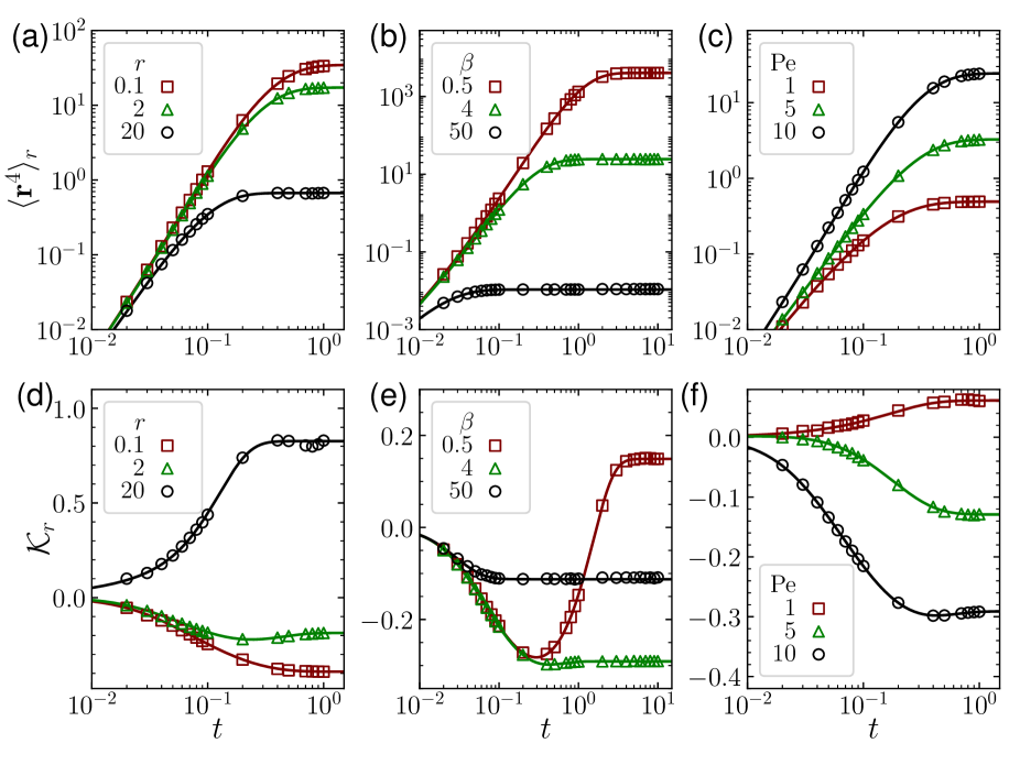
Figure 2: Time evolution of the fourth-order moment and excess kurtosis. (a), (b), (c) Fourth-order moment of displacement $\langle{\bf r}^{4}\rangle_{r}$ (equation (81)); (d), (e), (f) Kurtosis $\mathcal{K}_{r}$ as a function of time $t$ for different conditions: resetting rates $r=0.1,~{}2,~{}20$ with $\mathrm{Pe}=10$ and $\beta=4$ in (a) and (d); trapping strength $\beta=0.5,~{}4,~{}50$ with $\mathrm{Pe}=10$ and $r=1$ in (b) and (e); and activity $\mathrm{Pe}=1,~{}5,~{}10$ with $r=1$ and $\beta=4$ in (c) and (f). The solid lines represent analytic predictions, while points denote simulation results. The initial position is at the origin, with the initial orientation along the $x$-axis. The region where $\mathcal{K}_{r}<0$ (red) represents the activity-dominated regime, and $\mathcal{K}_{r}>0$ (green) represents the resetting-dominated regime.

4 Mean-squared displacement (MSD)

We proceed to compute mean-squared displacement $\langle{\bf r}^{2}\rangle_{s}$ defining observable $\psi={\bf r}^{2}$, utilizing equation (5) with initial position at origin $\langle{\bf r}^{2}\rangle_{0}=0$ leads to the mean-squared displacement in Laplace space $\langle{\bf r}^{2}\rangle_{s}$

$$\langle{\bf r}^{2}\rangle_{s} = \frac{1}{s+2\beta}\left[\frac{4}{s}+2\mathrm{Pe}\langle{\bf r}\cdot{\bf\hat{u}}\rangle_{s}\right]~{},$$ (10)

where the second term $\langle{\bf r}\cdot{\bf\hat{u}}\rangle_{s}$ calculated assuming $\psi={\bf r}\cdot{\bf\hat{u}}$ in equation (5) as

$$\langle{\bf r}\cdot{\bf\hat{u}}\rangle_{s}=\frac{\mathrm{Pe}}{s(s+\beta+1)}~{}.$$ (11)

Inverse Laplace transform of equation (10) gives mean-squared displacement $\langle{\bf r}^{2}(t)\rangle$ without stochastic resetting (see B), which previously obtained in Chaudhuri et al. [30]. Finally, using renewal approach in equation (6), we get

$$\langle{\bf r}^{2}(t)\rangle_{r}=e^{-rt}\left[\frac{2}{\beta}\left(1-e^{-2\beta t}\right)+\frac{\mathrm{Pe}^{2}}{\beta(1+\beta)}-\frac{2\mathrm{Pe}^{2}e^{-\beta t}}{1-\beta}\left[\frac{e^{-\beta t}}{2\beta}-\frac{e^{-t}}{1+\beta}\right]\right]$$

$$+\frac{(2+2\beta+\mathrm{Pe}^{2})(1-e^{-rt})}{\beta(1+\beta)}+\frac{2r\beta\mathrm{Pe}^{2}[1-e^{-(1+\beta+r)t}]}{(1+\beta+r)(1-\beta^{2})}+\frac{r(\mathrm{Pe}^{2}+2\beta-2)(1-e^{-(2\beta+r)t})}{\beta(2\beta+r)(1-\beta)}\,.$$

(12)

In figure 1(c), we compare the equation (12) represented by solid lines, with simulations depicted by points, showing excellent agreement. The various limiting cases of equation (12) depending on parameters $r$, $\mathrm{Pe}$, and $\beta$ discussed in B.

At small time ($t\to 0$), equation (12) leading to

$$\langle{\bf r}^{2}\rangle_{r}\simeq 4t+(\mathrm{Pe}^{2}-4\beta-2r)t^{2}+\frac{1}{3}\left[8\beta^{2}-\mathrm{Pe}^{2}-3\beta\mathrm{Pe}^{2}+8\beta r-2\mathrm{Pe}^{2}r+2r^{2}\right]t^{3}+\mathcal{O}(t^{4})\,.$$

The MSD at small time exhibits diffusive behavior $\langle{\bf r}^{2}\rangle_{r}=4t$, which crosses over to ballistic behavior $\langle{\bf r}^{2}\rangle_{r}\sim t^{2}$ when $\mathrm{Pe}^{2}>2r+4\beta$ at $t^{*}=4/(\mathrm{Pe}^{2}-2r-4\beta)$. In the steady state, MSD $\langle{\bf r}^{2}\rangle^{st}_{r}=\langle{\bf r}^{2}\rangle_{r}(t\to\infty)$ gives

$$\langle{\bf r}^{2}\rangle^{st}_{r} = \frac{4}{2\beta+r}+\frac{2\mathrm{Pe}^{2}}{(1+\beta+r)(2\beta+r)}~{}.$$ (14)

The standard deviation is given by $\sigma=\sqrt{\langle{\bf r}^{2}\rangle^{st}_{r}/2}$, the Gaussian probability distribution is $P(|{\bf r}|)=e^{-{\bf r}^{2}/2\sigma^{2}}/2\pi\sigma^{2}$. These are represented by solid lines in figures 3(d), 3(e), and 3(f).

The effective diffusion coefficient $D_{\rm eff}=(\beta+r)\langle{\bf r}^{2}\rangle_{\rm st}/2$

$$D_{\rm eff} = \frac{2(\beta+r)}{2\beta+r}+\frac{(\beta+r)\mathrm{Pe}^{2}}{(1+\beta+r)(2\beta+r)}\,.$$ (15)

Setting resetting $r=0$ and activity $\mathrm{Pe}=0$, $D_{\rm eff}=1$ holds the fluctuation dissipation relation (FDR). Excess diffusion coefficient due to non-equilibrium nature, calculated as $D_{\rm ex}=D_{\rm eff}-1$ reads

$$D_{\rm ex} = \frac{r}{2\beta+r}+\frac{(\beta+r)\mathrm{Pe}^{2}}{(1+\beta+r)(2\beta+r)}\,.$$ (16)

when $D_{\rm ex}=0$, the fluctuation-dissipation relation holds for $r=\mathrm{Pe}=0$. Both activity ($\mathrm{Pe}$) and resetting ($r$) breaks this relation and resulting in $D_{\rm ex}>0$. However, it is not possible to precisely distinguish between the activity-dominated and resetting-dominated regimes by calculating $D_{\rm ex}$ when varying the parameters $r,\beta,\mathrm{Pe}$. We distinguish them by calculating the excess kurtosis in the next section.

In the absence of stochastic resetting ($r=0$), we get ABP in a harmonic trap [30]. In the absence of activity ($\mathrm{Pe}=0$), Brownian particle in two dimensions under resetting gives $\langle{\bf r}^{2}\rangle^{st}_{r}=4/(2\beta+r)$, $D_{\rm eff}=2(\beta+r)/(2\beta+r)$, and $D_{\rm ex}=r/(2\beta+r)$.

Moreover, the displacement fluctuations and their limiting cases are discussed in C. The components of the second-order moment, such as those along the initial orientation direction, are also discussed in D.

5 Excess kurtosis: signature of non-Gaussian behavior

To calculate the excess kurtosis, we first need to calculate the fourth-order moment of the displacement. In the similar method, we calculated the fourth order moment of displacement under stochastic position and orientation resetting, detailed derivation and final result of $\langle{\bf r}^{4}(t)\rangle_{r}$ in equation (81), see detailed derivation in E. The small time expansion ($t\to 0$), the fourth moment of displacement $\langle{\bf r}^{4}\rangle_{r}$

$$\langle{\bf r}^{4}\rangle_{r}\simeq 32t^{2}+\frac{16}{3}\left(3\mathrm{Pe}^{2}-4r-12\beta\right)t^{3}$$

$$+\frac{1}{3}\left[224\beta^{2}+3\mathrm{Pe}^{4}+24r^{2}+144\beta r-96\beta\mathrm{Pe}^{2}-16\mathrm{Pe}^{2}-36r\mathrm{Pe}^{2}\right]t^{4}+\mathcal{O}(t^{5})\,,$$ (17)

exhibits small time diffusive behavior $\langle{\bf r}^{4}\rangle_{r}=32t^{2}$, which crosses over to ballistic behavior $\langle{\bf r}^{4}\rangle_{r}\sim t^{3}$ at $t^{*}=6/(3\mathrm{Pe}^{2}-4r-12\beta)$ with $\mathrm{Pe}^{2}>4(r+3\beta)/3$. In figures 2(a), 2(b), and 2(c), we have shown the $\langle{\bf r}^{4}\rangle_{r}$ as a function of time $t$ for resetting rates $r=0.1,~{}2,~{}20$ with $\mathrm{Pe}=10$ and $\beta=4$ in (a), for trap strength $\beta=0.5,~{}4,~{}50$ with $\mathrm{Pe}=10$ and $r=1$ in (b), and for activity $\mathrm{Pe}=1,~{}5,~{}10$ with $\beta=4$ and $r=1$ in (c). The solid lines are the plot of equation (81) which excellently agrees with the simulation results depicted by points. In figures 2(a) and 2(b), we can see the increase of resetting rates $r$ and trapping strengths $\beta$ decreases the $\langle{\bf r}^{4}\rangle_{r}$. On the other hand, the increase of activity parameter $\mathrm{Pe}$ increases the $\langle{\bf r}^{4}\rangle_{r}$. In the long time limit ($t\to\infty$), $\langle{\bf r}^{4}\rangle_{r}$ reaches a steady state due to the effect of the harmonic trap and/or stochastic resetting. The steady state fourth moment of displacement $\langle{\bf r}^{4}\rangle^{st}_{r}$

$$\langle{\bf r}^{4}\rangle^{st}_{r}=\frac{8}{(1+\beta+r)(2\beta+r)(4+2\beta+r)(1+3\beta+r)(4\beta+r)}\times$$

$$\left[48\beta^{3}+8(1+r)^{2}(4+r)+\mathrm{Pe}^{4}(8+3r)+8\beta^{2}(20+6\mathrm{Pe}^{2}+11r)\right.$$

$$\left.+4\mathrm{Pe}^{2}(8+14r+3r^{2})+2\beta\left[3\mathrm{Pe}^{4}+8\mathrm{Pe}^{2}(7+3r)+24(3+4r+r^{2})\right]\right]\,.$$ (18)

In order to quantify the impact of these parameters on position distributions at different times as well as in the steady state, we calculate excess kurtosis which define the deviation from a Gaussian process.

In the absence of activity ($\mathrm{Pe}=0$) and stochastic resetting ($r=0$), Brownian particle in two dimensions in a harmonic trap gives zero kurtosis which signifies the Gaussian process. We calculate the kurtosis in presence of activity and stochastic position and orientation resetting which deviates from zero. Thus, the non-equilibrium nature of the system leading to the deviation from Gaussian nature given by excess kurtosis [30],

$$\mathcal{K}_{r} = \frac{\langle{\bf r}^{4}\rangle_{r}}{2\langle{\bf r}^{2}\rangle_{r}^{2}}-1\,.$$ (19)

The fourth order moment of displacement $\langle{\bf r}^{4}\rangle_{r}$ and mean-squared displacement $\langle{\bf r}^{2}\rangle_{r}$ have already been calculated as shown in equation (81) and equation (12), respectively. We expand the kurtosis in the small time limit ($t\to 0$),

$$\mathcal{K}_{r} \simeq \frac{rt}{3}-\frac{(3\mathrm{Pe}^{4}+16\beta r-4r\mathrm{Pe}^{2})}{96}t^{2}+\mathcal{O}(t^{3})~{}.$$ (20)

The next order term $\mathcal{O}(t^{3})$ is shown in equation (86). It has shown the deviation of kurtosis towards positive or negative values in the small time controlled by $r$, $\mathrm{Pe}$, and $\beta$. The positive deviation holds for small activity ($\mathrm{Pe}\to 0$) but it deviates towards negative values with increase of activity. For high activity, the kurtosis deviates towards negative values at $t^{*}=32r/(3\mathrm{Pe}^{4}+16\beta r-4r\mathrm{Pe}^{2})$.

In figures 2(d), 2(e), and 2(f), we have shown the $\mathcal{K}_{r}$ as a function of time $t$ for resetting rates $r=0.1,~{}2,~{}20$ with $\mathrm{Pe}=10$ and $\beta=4$ in (d), for trapping strength $\beta=0.5,~{}4,~{}50$ with $\mathrm{Pe}=10$ and $r=1$ in (e), and for Péclet values $\mathrm{Pe}=1,~{}5,~{}10$ with $\beta=4$ and $r=1$ in (f). The solid lines are the plot of equation (19) which excellently agrees with the simulation results depicted by points. We characterize the activity- and resetting-dominated time regimes using excess kurtosis ($\mathcal{K}_{r}$). At short times, thermal diffusion leads to near-Gaussian behavior ($\mathcal{K}_{r}\sim 0$). Negative $\mathcal{K}_{r}$ indicates a flat, light-tailed with non-zero peak at $\mathrm{Pe}/\beta$ position distribution dominated by activity ($\mathrm{Pe}$), while positive $\mathcal{K}_{r}$ suggests a heavy-tailed with peak at zero position distribution dominated by resetting ($r$). In figure 2(d), we clearly observe activity-dominated behavior ($\mathcal{K}_{r}<0$) at low resetting rates ($r$) and resetting-dominated behavior ($\mathcal{K}_{r}>0$) at high resetting rates ($r$). In figure 2(e), we observe non-monotonic behavior at small trap strength ($\beta$). At short times, $\mathcal{K}_{r}$ shifts to negative values, indicating activity-dominated behavior, crosses zero at intermediate times, and eventually saturates to positive values, reflecting long-term resetting-dominated behavior. The transitions from small to long times are: Gaussian ($\mathcal{K}_{r}=0$) to light-tail ($\mathcal{K}_{r}<0$), back to Gaussian ($\mathcal{K}_{r}=0$), and finally to heavy-tail ($\mathcal{K}_{r}>0$) position distributions. In figure 2(f), we observe activity-dominated behavior ($\mathcal{K}_{r}<0$) at high activity ($\mathrm{Pe}$) and resetting-dominated behavior ($\mathcal{K}_{r}>0$) at low activity ($\mathrm{Pe}$).

To quantify the steady-state properties of position distributions and capture the transitions between activity- and resetting-dominated regions, we calculate the steady-state excess kurtosis and analyze the numerically obtained position distributions.

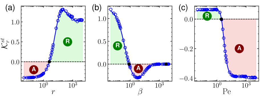
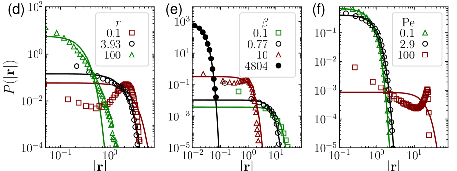
Figure 3: Steady-state kurtosis, $\mathcal{K}^{st}_{r}$, as a function of $r$ with $\mathrm{Pe}=10$ and $\beta=4$ in (a), $\beta$ with $\mathrm{Pe}=10$ and $r=1$ in (b), and $\mathrm{Pe}$ with $r=1$ and $\beta=4$ in (c). The blue solid line represents the exact analytical solution for steady-state kurtosis as given by equation (21). The symbols (blue open circles) are from simulation results. The regions where $\mathcal{K}^{st}_{r}<0$ (red) correspond to the activity (A)-dominated regime, while regions where $\mathcal{K}^{st}_{r}>0$ (green) correspond to the resetting (R)-dominated regime. The critical points where $\mathcal{K}^{st}_{r}=0$ (black solid symbols) occur at $r_{c}=3.93$ in (a), $\beta^{I}_{c}=0.77$ and $\beta^{II}_{c}=4804$ in (b), and $\mathrm{Pe}_{c}=2.90$ in (c). The radial probability distributions for three resetting rates in (d) correspond to (a), four harmonic trap strengths in (e) to (b), and three activity values in (f) to (c).

6 Steady state excess kurtosis and phase diagrams

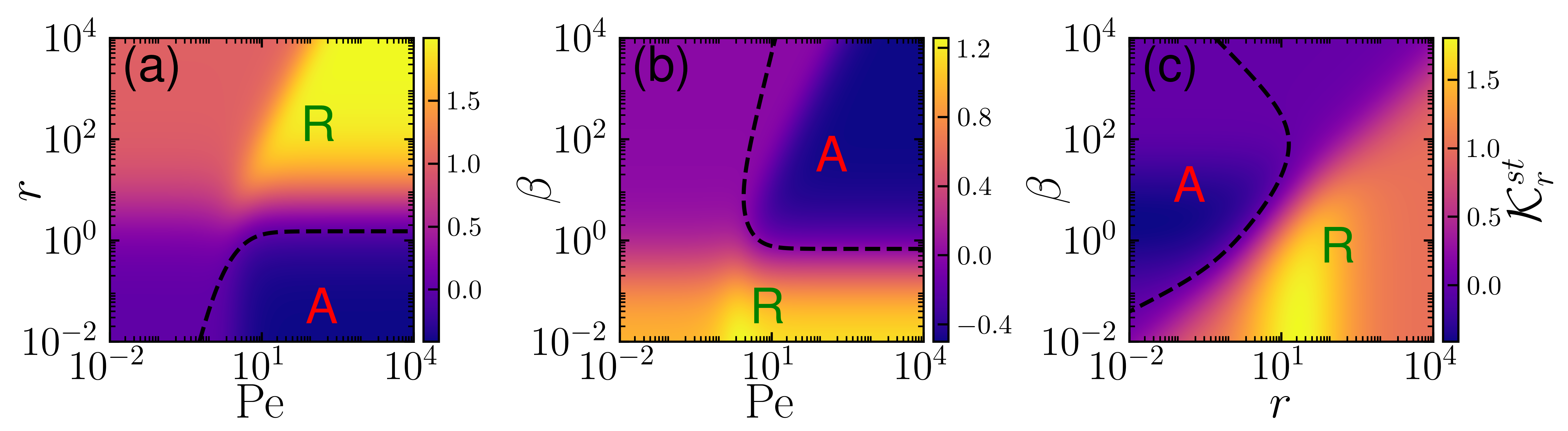
Figure 4: Phase Diagrams. Steady-state kurtosis, $\mathcal{K}^{st}_{r}$, is shown in the $\mathrm{Pe}-r$ plane with $\beta=1$ in (a), in the $\mathrm{Pe}-\beta$ plane with $r=1$ in (b), and in the $r-\beta$ plane with $\mathrm{Pe}=10$ in (c). The black dashed line corresponds to $\mathcal{K}^{st}_{r}=0$. The region where $\mathcal{K}^{st}_{r}<0$ is denoted as the activity-dominated regime (A), and the region where $\mathcal{K}^{st}_{r}>0$ is denoted as the resetting-dominated regime (R).

In the steady state($t\to\infty$), equation (19) results

$$\mathcal{K}^{st}_{r}=\frac{2}{(4+2\beta+r)(1+3\beta+r)(4\beta+r)(2+2\beta+\mathrm{Pe}^{2}+2r)^{2}}\times$$

$$\left[12\beta^{4}r-\beta^{3}(6\mathrm{Pe}^{4}-20\mathrm{Pe}^{2}r-2r(26+17r))\right.$$

$$\left.+r(1+r)(\mathrm{Pe}^{4}(2+r)+2(1+r)^{2}(4+r)+2\mathrm{Pe}^{2}(2r^{2}+9r+4))\right.$$

$$\left.+\beta^{2}(-\mathrm{Pe}^{4}(14+r)+2\mathrm{Pe}^{2}r(32+19r)+2r(17r^{2}+55r+38))\right.$$

$$\left.+\beta r(\mathrm{Pe}^{4}(1+3r)+2(1+r^{2})(22+7r)+\mathrm{Pe}^{2}(22r^{2}+80r+52))\right]\,.$$ (21)

We now calculate various limiting cases to explore the properties of excess kurtosis. I. Brownian particles in a harmonic trap : In the absence of activity ($\mathrm{Pe}=0$) and stochastic resetting ($r=0$), Brownian particle in two dimensions in a harmonic trap gives $\mathcal{K}_{r}^{st}=0$. It signifies the Gaussian process, and we calculate the steady state kurtosis to quantify the deviation from $\mathcal{K}_{r}^{st}=0$.

II. Brownian particles under stochastic resetting : In the absence of activity ($\mathrm{Pe}=0$) and harmonic trap ($\beta=0$), Brownian particle in two dimensions under stochastic position and orientation resetting gives $\mathcal{K}^{st}_{r}=1$. The positive kurtosis signifies the heavy tailed position distribution at long times.

III. Brownian particles under stochastic resetting in a harmonic trap : In the absence of activity ($\mathrm{Pe}=0$), Brownian particles in two dimensions under stochastic position and orientation resetting in a harmonic trap gives $\mathcal{K}^{st}_{r}=r/(4\beta+r)$. It suggests the decrease of kurtosis with the increase of trapping strength $\beta$. For very high resetting rates, $\mathcal{K}^{st}_{r}$ reaches a maximum value of $1$.

IV. ABP under stochastic resetting : In the absence of harmonic trap ($\beta=0$), ABP under complete stochastic resetting, equation (21) gives,

$$\mathcal{K}^{st}_{r}=\frac{\left[4(1+r)^{2}(4+r)+4(2r^{2}+9r+4)\mathrm{Pe}^{2}+2(2+r)\mathrm{Pe}^{4}\right]}{(4+r)(2(1+r)+\mathrm{Pe}^{2})^{2}}~{}.$$ (22)

Remarkably, in the absence of a harmonic trap ($\beta=0$), equation (22) yields only positive values, indicating heavy-tailed position distributions (see G).

V. ABP in a harmonic trap : In the absence of stochastic resetting ($r=0$), ABP in a harmonic trap gives the steady state kurtosis $\mathcal{K}^{st}$ already explored in [30].

In figures 3(a), 3(b), and 3(c), the steady state kurtosis $\mathcal{K}^{st}_{r}$ from equation (21) is shown as blue solid lines, compared with simulation results represented by blue open points. The black solid points denote the Gaussian behavior at $\mathcal{K}^{st}_{r}=0$. The negative kurtosis $\mathcal{K}^{st}_{r}<0$ indicates persistent active motion, leading to a flat, light-tailed position distribution with a non-zero peak. This is referred to as the activity (A) dominated regime. Positive kurtosis, $\mathcal{K}^{st}_{r}>0$, indicates passive motion, resulting in a narrow, heavy-tailed position distribution peaking at zero. This is referred to as the resetting (R) dominated regime. In figures 3(d), 3(e), and 3(f), we plot the radial distribution from simulations (points) alongside the corresponding Gaussian distribution (solid lines) using the second-order moment.

Figure 3(a) shows a monotonic transition from the activity (A) dominated regime at small resetting rates ($r$) to the resetting (R) dominated regime at larger resetting rates, with a critical resetting rate ($r_{c}$) marking Gaussian behavior. Interestingly, in the resetting dominated regime, the steady-state kurtosis $\mathcal{K}^{st}_{r}$ exhibits a non-monotonic transition, reaching its maximum positive value at intermediate $r$. This is purely due to the interplay between activity ($\mathrm{Pe}$) and resetting ($r$), which occurs even in the absence of a harmonic trap (see G). In figure 3(d), we present the radial distribution for three resetting rates: the activity-dominated regime at $r<r_{c}$, Gaussian behavior at $r=r_{c}$, and the resetting-dominated regime at $r>r_{c}$.

Figure 3(b) shows a non-monotonic transition as a function of trap strength $\beta$. Initially, the resetting (R) dominated regime occurs at weak trap strength, transitioning to the activity (A) dominated regime at stronger trap strengths, with a critical trap strength ($\beta^{I}_{c}$) indicating Gaussian behavior. Subsequently, the activity (A) dominated regime transitions back to the resetting regime at very strong trap strengths, marked by another critical trap strength ($\beta^{II}_{c}$). In figure 3(e), we present the radial distribution for four trap strengths: the resetting-dominated regime at $\beta<\beta_{c}$, Gaussian behavior at $\beta=\beta^{I}_{c}$, the activity-dominated regime at $\beta>\beta_{c}$, Gaussian behavior at $\beta=\beta^{II}_{c}$. In the resetting-dominated regime for $\beta>\beta^{II}_{c}$, the steady-state kurtosis $\mathcal{K}^{st}_{r}$ takes very small positive values, making the heavy-tail visualization nearly impossible.

Figure 3(c) shows a monotonic transition from the resetting (R) dominated regime at small activity ($\mathrm{Pe}$) to the activity (A) dominated regime at larger activity, with a critical resetting rate ($\mathrm{Pe}_{c}$) marking Gaussian behavior. In figure 3(f), we present the radial distribution for three activity ($\mathrm{Pe}$) values: the resetting-dominated regime at $\mathrm{Pe}<\mathrm{Pe}_{c}$, Gaussian behavior at $\mathrm{Pe}=\mathrm{Pe}_{c}$, and the activity-dominated regime at $\mathrm{Pe}>\mathrm{Pe}_{c}$.

In figures 4(a), 4(b), and 4(c), we plot the phase diagram considering $\mathcal{K}^{st}_{r}$ as order parameter to show the activity (A) and resetting (R) dominated regime separating by Gaussian line $\mathcal{K}^{st}_{r}=0$ depicted by black dashed line. Figure 4(a) shows the phase diagram in the $\mathrm{Pe}$-$r$ plane, highlighting two key points: at small resetting rates ($r$), the transition progresses from weak resetting (R) to Gaussian, then to the activity (A) dominated regime. At large resetting rates, increasing activity enhances the resetting (R) dominated regime, resulting in a heavier tail in the distribution. Figure 4(b) shows the phase diagram in the $\mathrm{Pe}$-$\beta$ plane, highlighting a re-entrant transition with increasing trap strength ($\beta$), progressing from resetting (R) to Gaussian, then to activity (A), back to Gaussian, and finally returning to resetting-dominated behavior. The suppression of resetting behavior with increasing trap strength in figure 4(b) is also illustrated in the $r$-$\beta$ plane in figure 4(c).

7 Conclusions

In this work, we computed the exact analytical moments of a two-dimensional Active Brownian Particle (ABP) subject to complete stochastic resetting (both position and orientation) in a harmonic trap. These analytical results were validated against numerical simulations, demonstrating excellent agreement, and the nonequilibrium steady-state behavior was thoroughly analyzed.

In the steady state, the orientation autocorrelation decays to a non-zero value in the presence of resetting, increasing with the resetting rate and approaching unity as the resetting rate becomes large. The steady state mean displacement exhibits non-monotonic behavior with resetting rate, initially increasing from zero as the resetting rate rises, peaking, and then returning to near-zero at very high resetting rates. We showed that ballistic dynamics emerge in the mean squared displacement (MSD) at intermediate times with increasing activity, though these are suppressed when resetting dominates. Additionally, the MSD reveals that the fluctuation-dissipation relation (FDR) holds in the absence of both activity and resetting, but breaks down, yielding a non-zero excess diffusion coefficient, when either is present.

To distinguish between the activity-dominated (A) and resetting-dominated (R) regimes, we computed the fourth moment of displacement and the corresponding excess kurtosis, providing a complete characterization of the system. In the steady state, excess kurtosis captures the transition between the activity-dominated regime (negative excess kurtosis) and the resetting-dominated regime (positive excess kurtosis), with the Gaussian regime represented by zero excess kurtosis. We anticipate that this rich steady-state behavior can be experimentally validated in active colloids or robotic systems, as shown in [79]. In the future, it will be crucial to explore Active Brownian Particles (ABPs) under two additional stochastic resetting protocols, only position resetting and only orientation resetting in a harmonic trap, to gain valuable insights into optimal resetting strategies in external potentials.

Appendix A Orientation autocorrelation and mean displacement without harmonic trap

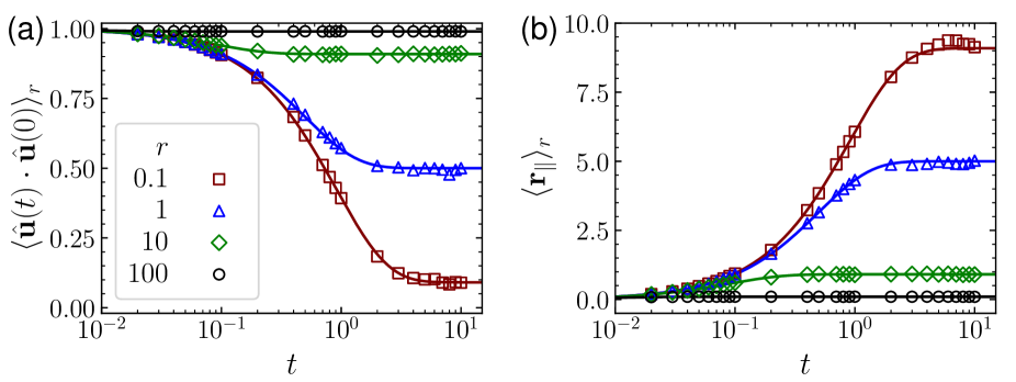
Figure 5: (a) Orientation autocorrelation (equation (7)) and (b) mean parallel displacement (equation (8)) as a function of time in two dimension for $r=0.1(\mathrm{square},\Box),~{}1(\mathrm{triangle},\triangle),~{}10(\mathrm{diamond},\Diamond),~{}100(\mathrm{circle},\circ)$ with $\beta=0$ and $\mathrm{Pe}=10$. Points are from simulation results and solid lines are analytic plot. The initial position is at the origin with the initial orientation along the $x$-axis.

In figure 5(a), we plot the orientation autocorrelation from equation (7) for varying resetting rates ($r$). As the resetting rate increases, the orientation autocorrelation saturates at higher, non-zero values. In figure 5(b), we plot the mean parallel displacement as a function of time from equation (8) for varying resetting rates ($r$) with activity $\mathrm{Pe}=10$ in the absence of a harmonic trap ($\beta=0$).

Appendix B Limiting cases of mean-squared displacement (MSD)

B.1 ABP in a harmonic trap

Inverse Laplace transform of equation (10) gives mean-squared displacement $\langle{\bf r}^{2}(t)\rangle$ for an ABP in a harmonic trap without stochastic resetting (or by setting $r=0$ in equation (12)), previously calculated by Chaudhuri et al. [30],

$$\langle{\bf r}^{2}(t)\rangle = \frac{2}{\beta}\left(1-e^{-2\beta t}\right)+\frac{\mathrm{Pe}^{2}}{\beta(1+\beta)}-\frac{2\mathrm{Pe}^{2}e^{-\beta t}}{1-\beta}\left[\frac{e^{-\beta t}}{2\beta}-\frac{e^{-t}}{1+\beta}\right]\,.$$ (23)

At small times ($t\to 0$), the expansion of equation (23) leads to

$$\langle{\bf r}^{2}\rangle \simeq 4t+(\mathrm{Pe}^{2}-4\beta)t^{2}+\frac{1}{3}\left[8\beta^{2}-\mathrm{Pe}^{2}-3\beta\mathrm{Pe}^{2}\right]t^{3}+\mathcal{O}(t^{4})\,.$$ (24)

In the steady state ($t\to\infty$), equation (23) gives

$$\langle{\bf r}^{2}\rangle^{st} = \frac{2}{\beta}+\frac{\mathrm{Pe}^{2}}{\beta(1+\beta)}\,.$$ (25)

The effective diffusion coefficient $D_{\rm eff}=\beta\langle{\bf r}^{2}\rangle_{\rm st}/2$

$$D_{\rm eff}=1+\frac{\mathrm{Pe}^{2}}{2(1+\beta)}\,,$$ (26)

which enhanced with increase of activity $\mathrm{Pe}$ and suppressed with increase of harmonic stiffness $\beta$.

B.2 ABP under complete stochastic resetting

In the absence of harmonic trap ($\beta=0$), equation (12) simplifies to

$$\langle{\bf r}^{2}(t)\rangle_{r} = \frac{4(1+r)+2\mathrm{Pe}^{2}}{r(1+r)}-\frac{(4+2\mathrm{Pe}^{2})e^{-rt}}{r}+\frac{2\mathrm{Pe}^{2}e^{-(1+r)t}}{(1+r)}\,.$$ (27)

At small times ($t\to 0$), the expansion of equation (27) leads to

$$\langle{\bf r}^{2}(t)\rangle_{r} \simeq 4t+(\mathrm{Pe}^{2}-2r)t^{2}-\frac{1}{3}\left[\mathrm{Pe}^{2}(1+2r)-2r^{2}\right]t^{3}+\mathcal{O}(t^{4})\,.$$ (28)

The MSD at small time exhibits diffusive behavior $\langle{\bf r}^{2}\rangle_{r}=4t$, which crosses over to ballistic behavior $\langle{\bf r}^{2}\rangle_{r}\sim t^{2}$ when $\mathrm{Pe}^{2}>2r$ at $t^{*}=4/(\mathrm{Pe}^{2}-2r)$. At long times ($t\to\infty$), $\langle{\bf r}^{2}\rangle_{r}$ reaches a steady state,

$$\langle{\bf r}^{2}\rangle^{st}_{r} = \frac{4}{r}+\frac{2\mathrm{Pe}^{2}}{r(1+r)}~{}.$$ (29)

It reaches steady state at $t^{st}=\langle{\bf r}^{2}\rangle^{st}_{r}/4$ for $\mathrm{Pe}^{2}\leq 2r$ and $t^{st}=[\langle{\bf r}^{2}\rangle^{st}_{r}/(\mathrm{Pe}^{2}-2r)]^{1/2}$ for $\mathrm{Pe}^{2}>2r$.

Note, the steady-state MSD in equations (29) and (25) have same form, with $\langle{\bf r}^{2}\rangle^{st}_{r}=2\langle{\bf r}^{2}\rangle^{st}$. Thus, in the steady state, the impact of stochastic resetting rate and trap stiffness on ABP is equivalent.

The effective diffusion coefficient $D_{\rm eff}=r\langle{\bf r}^{2}\rangle_{\rm st}/2$

$$D_{\rm eff}=2\left[1+\frac{\mathrm{Pe}^{2}}{2(1+r)}\right]\,.$$ (30)

This is twice the effective diffusion coefficient of ABP in a harmonic trap. Similar to ABP in a harmonic trap, the effective diffusion coefficient here is enhanced with an increase in activity $\mathrm{Pe}$ and suppressed with increase of resetting rate $r$.

B.3 Brownian particle under stochastic resetting in harmonic trap

In the absence of activity ($\mathrm{Pe}=0$), equation (12) simplifies to

$$\langle{\bf r}^{2}(t)\rangle_{r}=\frac{4\left(1-e^{-(2\beta+r)t}\right)}{2\beta+r}\,.$$ (31)

At small times ($t\to 0$), the expansion of equation (31) leads to

$$\langle{\bf r}^{2}\rangle_{r}\simeq 4t-2(2\beta+r)t^{2}+\frac{2}{3}\left[4\beta^{2}+4\beta r+r^{2}\right]t^{3}+\mathcal{O}(t^{4})\,.$$ (32)

The MSD at small time exhibits diffusive behavior $\langle{\bf r}^{2}\rangle_{r}=4t$, which reaches steady state ($t\to\infty$), equation (31) gives

$$\langle{\bf r}^{2}\rangle^{st}_{r}=\frac{4}{(2\beta+r)}\,.$$ (33)

The effective diffusion coefficient $D_{\rm eff}=(\beta+r)\langle{\bf r}^{2}\rangle_{\rm st}/2$

$$D_{\rm eff}=\frac{2(\beta+r)}{(2\beta+r)}\,.$$ (34)

The effective diffusion coefficient increases with increase of resetting rate $r$.

B.4 Brownian particle under stochastic resetting

In the absence of activity ($\mathrm{Pe}=0$) and harmonic trap ($\beta=0$), equation (12) simplifies to

$$\langle{\bf r}^{2}(t)\rangle_{r}=\frac{4\left(1-e^{-rt}\right)}{r}\,.$$ (35)

At small times ($t\to 0$), the expansion of equation (35) leads to

$$\langle{\bf r}^{2}\rangle_{r}\simeq 4t-2rt^{2}+\frac{2}{3}r^{2}t^{3}+\mathcal{O}(t^{4})\,.$$ (36)

In the steady state ($t\to\infty$), equation (35) gives

$$\langle{\bf r}^{2}\rangle^{st}_{r}=\frac{4}{r}\,.$$ (37)

The effective diffusion coefficient $D_{\rm eff}=r\langle{\bf r}^{2}\rangle_{\rm st}/2$

$$D_{\rm eff}=2\,.$$ (38)

The effective diffusion coefficient is constant and twice of the thermal diffusion coefficient.

Appendix C Displacement fluctuations and its limiting cases

The displacement fluctuation $\langle\delta{\bf r}^{2}\rangle_{r}=\langle{\bf r}^{2}\rangle_{r}-\langle{\bf r}\rangle_{r}^{2}$. At small time ($t\to 0$),

$$\langle\delta{\bf r}^{2}\rangle_{r} \simeq 4t-2(2\beta+r)t^{2}+\frac{2}{3}\left[4\beta^{2}+\mathrm{Pe}^{2}+4\beta r+r^{2}\right]t^{3}+\mathcal{O}(t^{4})\,.$$ (39)

In the steady state,

$$\langle\delta{\bf r}^{2}\rangle^{st}_{r} = \frac{4[2+\mathrm{Pe}^{2}+3r+r^{2}+2\beta+\beta r]}{(2+r)(1+\beta+r)(2\beta+r)}\,.$$ (40)

The limiting cases are discussed below.

C.1 ABP in a harmonic trap

The displacement fluctuation $\langle\delta{\bf r}^{2}\rangle=\langle{\bf r}^{2}\rangle-\langle{\bf r}\rangle^{2}$. Here, we set resetting rate $r=0$.

At small times ($t\to 0$),

$$\langle\delta{\bf r}^{2}\rangle \simeq 4t-4\beta t^{2}+\frac{2}{3}\left[4\beta^{2}+\mathrm{Pe}^{2}\right]t^{3}+\mathcal{O}(t^{4})\,.$$ (41)

In the steady state ($t\to\infty$),

$$\langle\delta{\bf r}^{2}\rangle^{st} = \frac{2}{\beta}+\frac{\mathrm{Pe}^{2}}{\beta(1+\beta)}\,.$$ (42)

C.2 ABP under complete stochastic resetting

The displacement fluctuation $\langle\delta{\bf r}^{2}\rangle_{r}=\langle{\bf r}^{2}\rangle_{r}-\langle{\bf r}\rangle_{r}^{2}$. Here, we set trap strength $\beta=0$.

At small times ($t\to 0$),

$$\langle\delta{\bf r}^{2}\rangle_{r} \simeq 4t-2rt^{2}+\frac{2}{3}\left(\mathrm{Pe}^{2}+r^{2}\right)t^{3}+\mathcal{O}(t^{4})\,.$$ (43)

In the steady state ($t\to\infty$),

$$\langle\delta{\bf r}^{2}\rangle^{st}_{r} = \frac{4}{r}+\frac{4\mathrm{Pe}^{2}}{r(1+r)(2+r)}\,.$$ (44)

C.3 Brownian particles under stochastic resetting in a harmonic trap

Here, we set activity $\mathrm{Pe}=0$. The displacement fluctuation $\langle\delta{\bf r}^{2}\rangle_{r}=\langle{\bf r}^{2}\rangle_{r}-\langle{\bf r}\rangle_{r}^{2}=\langle{\bf r}^{2}\rangle_{r}$.

C.4 Brownian particles under stochastic resetting

Here, we set activity $\mathrm{Pe}=0$ and trap strength $\beta=0$. The displacement fluctuation $\langle\delta{\bf r}^{2}\rangle_{r}=\langle{\bf r}^{2}\rangle_{r}-\langle{\bf r}\rangle_{r}^{2}=\langle{\bf r}^{2}\rangle_{r}$.

Appendix D Second order moment and fluctuations along initial orientation direction

D.1 ABP in a harmonic trap

The initial orientation of the ABP along $x$-direction ${\bf\hat{u}}_{0}=\hat{x}$. Using $\psi=r_{\parallel}^{2}=x^{2}$, we get using equation (5),

$$(s+2\beta)\langle r_{\parallel}^{2}\rangle_{s} = 2/s+2\mathrm{Pe}\langle xu_{x}\rangle_{s}\,.$$ (45)

Now, we proceed to calculate the second term $\langle xu_{x}\rangle_{s}$ assuming $\psi=xu_{x}$, we get using equation (5),

$$\langle xu_{x}\rangle = \frac{\mathrm{Pe}\langle u_{x}^{2}\rangle_{s}}{s+1+\beta}\,.$$ (46)

Again, we need to calculate $\langle u_{x}^{2}\rangle_{s}$, substituting $\psi=u_{x}^{2}$ in equation (5), we get

$$\langle u_{x}^{2}\rangle_{s} = \frac{s+2}{s(s+4)}\,.$$ (47)

Finally,

$$\langle r_{\parallel}^{2}\rangle_{s} = \frac{1}{(s+2\beta)}\left[\frac{2}{s}+\frac{2\mathrm{Pe}^{2}(s+2)}{s(s+4)(s+1+\beta)}\right]\,.$$ (48)

Inverse Laplace transformation of the above equation leads to the $\langle r_{\parallel}^{2}(t)\rangle$ for ABP in a harmonic trap in the absence of stochastic resetting

$$\langle r_{\parallel}^{2}(t)\rangle=\frac{e^{-4t}\mathrm{Pe}^{2}}{2(-3+\beta)(-2+\beta)}-\frac{2e^{-(1+\beta)t}\mathrm{Pe}^{2}}{(-3+\beta)(1+\beta)}+\frac{e^{-2\beta t}(2-\beta+\mathrm{Pe}^{2})}{(-2+\beta)\beta}+\frac{2+2\beta+\mathrm{Pe}^{2}}{2\beta(1+\beta)}\,.$$

In the small time limit ($t\to 0$), $\langle r_{\parallel}^{2}(t)\rangle$ gives

$$\langle r_{\parallel}^{2}(t)\rangle\simeq 2t+(-2\beta+\mathrm{Pe}^{2})t^{2}+\frac{1}{3}\left(4\beta^{2}-3\mathrm{Pe}^{2}-3\beta\mathrm{Pe}^{2}\right)t^{3}+\mathcal{O}(t^{4})\,.$$ (50)

In the steady state ($t\to\infty$), we get

$$\langle r_{\parallel}^{2}\rangle^{st} = \frac{2(1+\beta)+\mathrm{Pe}^{2}}{2\beta(1+\beta)}\,.$$ (51)

Displacement fluctuations along parallel direction $\langle\delta r_{\parallel}^{2}\rangle_{r}=\langle r_{\parallel}^{2}\rangle_{r}-\langle r_{\parallel}\rangle^{2}_{r}$.

$$\langle\delta r_{\parallel}^{2}(t)\rangle_{r} =\frac{1}{2}\left(\frac{e^{-4t}\mathrm{Pe}^{2}}{6-5\beta+\beta^{2}}-\frac{4e^{-(1+\beta)t}\mathrm{Pe}^{2}}{(-3+\beta)(1+\beta)}-\frac{2(e^{-t}-e^{-\beta t})^{2}\mathrm{Pe}^{2}}{(-1+\beta)^{2}}\right.$$ (52)

$$\left.+\frac{2e^{-2\beta t}(2-\beta+\mathrm{Pe}^{2})}{(-2+\beta)\beta}+\frac{2+2\beta+\mathrm{Pe}^{2}}{\beta+\beta^{2}}\right)\,.$$

In the small time limit ($t\to 0$), $\langle r_{\parallel}^{2}(t)\rangle_{r}$ gives

$$\langle\delta r_{\parallel}^{2}(t)\rangle_{r} \simeq 2t-2\beta t^{2}+\frac{4\beta^{2}t^{3}}{3}+\mathcal{O}(t^{4})\,.$$ (53)

In the steady state ($t\to\infty$), we get

$$\langle\delta r_{\parallel}^{2}\rangle_{r}^{st}=\langle r_{\parallel}^{2}\rangle^{st}=\frac{2(1+\beta)+\mathrm{Pe}^{2}}{2\beta(1+\beta)}\,.$$ (54)

Now the perpendicular component of displacement fluctuation $\langle\delta r_{\perp}^{2}\rangle_{r}=\langle\delta{\bf r}^{2}\rangle_{r}-\langle\delta r_{\parallel}^{2}\rangle_{r}$.

$$\langle\delta r_{\perp}^{2}(t)\rangle_{r} =-\frac{e^{-4t}\mathrm{Pe}^{2}}{2(6-5\beta+\beta^{2})}+\frac{4e^{-(1+\beta)t}\mathrm{Pe}^{2}}{3-\beta-3\beta^{2}+\beta^{3}}+\frac{2+2\beta+\mathrm{Pe}^{2}}{2\beta+2\beta^{2}}$$ (55)

$$-\frac{e^{-2\beta t}(2-3\beta+\beta^{2}+\mathrm{Pe}^{2})}{\beta(2-3\beta+\beta^{2})}\,.$$

In the small time limit ($t\to 0$), $\langle r_{\parallel}^{2}(t)\rangle_{r}$ gives

$$\langle\delta r_{\perp}^{2}(t)\rangle\simeq 2t-2\beta t^{2}+\frac{2}{3}(2\beta^{2}+\mathrm{Pe}^{2})t^{3}-\frac{1}{6}\left[4\beta^{3}+5\mathrm{Pe}^{2}+3\beta\mathrm{Pe}^{2}\right]t^{4}+\mathcal{O}(t^{5})\,.$$ (56)

In the steady state ($t\to\infty$), we get

$$\langle\delta r_{\perp}^{2}\rangle_{r}^{st}=\langle\delta r_{\parallel}^{2}\rangle^{st}_{r}=\langle r_{\parallel}^{2}\rangle^{st}=\frac{2(1+\beta)+\mathrm{Pe}^{2}}{2\beta(1+\beta)}\,.$$ (57)

D.2 ABP under stochastic resetting in a harmonic trap

Now, we get the $\langle r_{\parallel}^{2}(t)\rangle$ under stochastic position and orientation resetting using equation (6)

$$\langle r_{\parallel}^{2}(t)\rangle_{r}=e^{-rt}\left(\frac{e^{-4t}\mathrm{Pe}^{2}}{2(-3+\beta)(-2+\beta)}-\frac{2e^{-(1+\beta)t}\mathrm{Pe}^{2}}{(-3+\beta)(1+\beta)}+\frac{e^{-2\beta t}(2-\beta+\mathrm{Pe}^{2})}{(-2+\beta)\beta}+\frac{2+2\beta+\mathrm{Pe}^{2}}{2\beta(1+\beta)}\right)$$

$$+\frac{\beta(2-2e^{-rt})-e^{-(2\beta+r)t}(-1+e^{2\beta t})r}{\beta(2\beta+r)}+\frac{r\mathrm{Pe}^{2}}{2}\left[-\frac{e^{-(4+r)t}}{(6-5\beta+\beta^{2})(4+r)}+\frac{4e^{-(1+\beta+r)t}}{(-3+\beta)(1+\beta)(1+\beta+r)}\right.$$

$$\left.-\frac{2e^{-(2\beta+r)t}}{(-2+\beta)\beta(2\beta+r)}+\frac{4(2+r)}{r(4+r)(1+\beta+r)(2\beta+r)}-\frac{e^{-rt}}{\beta r+\beta^{2}r}\right]\,.$$ (58)

In the small time limit ($t\to 0$), $\langle r_{\parallel}^{2}(t)\rangle_{r}$ gives

$$\langle r_{\parallel}^{2}(t)\rangle\simeq 2t+(-2\beta+\mathrm{Pe}^{2}-r)t^{2}+\frac{1}{3}\left(4\beta^{2}-3\mathrm{Pe}^{2}-3\beta\mathrm{Pe}^{2}+4\beta r-2\mathrm{Pe}^{2}r+r^{2}\right)t^{3}$$

$$+\mathcal{O}(t^{4})\,.$$ (59)

In the steady state ($t\to\infty$), we get

$$\langle r_{\parallel}^{2}\rangle_{r}^{st} = \frac{2[(1+r)(4+r)+\mathrm{Pe}^{2}(2+r)+\beta(4+r)]}{(4+r)(1+\beta+r)(2\beta+r)}\,.$$ (60)

Displacement fluctuations along parallel direction $\langle\delta r_{\parallel}^{2}\rangle_{r}=\langle r_{\parallel}^{2}\rangle_{r}-\langle r_{\parallel}\rangle^{2}_{r}$.

$$\langle\delta r_{\parallel}^{2}(t)\rangle_{r}=\frac{1}{2}\left[e^{-rt}\left(\frac{e^{-4t}\mathrm{Pe}^{2}}{6-5\beta+\beta^{2}}-\frac{4e^{-(1+\beta)t}\mathrm{Pe}^{2}}{(-3+\beta)(1+\beta)}+\frac{2e^{-2\beta t}(2-\beta+\mathrm{Pe}^{2})}{(-2+\beta)\beta}+\frac{2+2\beta+\mathrm{Pe}^{2}}{\beta+\beta^{2}}\right)\right.$$

$$\left.-\frac{2\mathrm{Pe}^{2}(r-\beta r+\beta e^{-(\beta+r)t}(1+r)-e^{-(1+r)t}(\beta+r))^{2}}{(-1+\beta)^{2}(1+r)^{2}(\beta+r)^{2}}\right.$$

$$\left.+\mathrm{Pe}^{2}r\left(-\frac{e^{-(4+r)t}}{(6-5\beta+\beta^{2})(4+r)}+\frac{4e^{-(1+\beta+r)t}}{(-3+\beta)(1+\beta)(1+\beta+r)}-\frac{2e^{-(2\beta+r)t}}{(-2+\beta)\beta(2\beta+r)}\right.\right.$$

$$\left.\left.+\frac{4(2+r)}{r(4+r)(1+\beta+r)(2\beta+r)}-\frac{e^{-rt}}{\beta r+\beta^{2}r}\right)+\frac{\beta(4-4e^{-rt})-4e^{-(\beta+r)t}r\sinh(\beta t)}{\beta(2\beta+r)}\right]\,.$$ (61)

In the small time limit ($t\to 0$), $\langle r_{\parallel}^{2}(t)\rangle_{r}$ gives

$$\langle\delta r_{\parallel}^{2}(t)\rangle\simeq 2t-(2\beta+r)t^{2}+\frac{1}{3}\left(4\beta^{2}+4\beta r+\mathrm{Pe}^{2}r+r^{2}\right)t^{3}+\mathcal{O}(t^{4})\,.$$ (62)

In the steady state ($t\to\infty$), we get

$$\langle\delta r_{\parallel}^{2}\rangle_{r}^{st}=-\frac{\mathrm{Pe}^{2}r^{2}}{(1+r)^{2}(\beta+r)^{2}}+\frac{2}{2\beta+r}+\frac{2\mathrm{Pe}^{2}(2+r)}{(4+r)(1+\beta+r)(2\beta+r)}\,.$$ (63)

D.3 ABP under stochastic resetting

$$\langle r_{\parallel}^{2}(t)\rangle_{r}=\frac{e^{-(4+r)t}}{3r(1+r)(4+r)}\left(\mathrm{Pe}^{2}r(1+r)+2e^{3t}\mathrm{Pe}^{2}r(4+r)-3e^{4t}(2+\mathrm{Pe}^{2})(1+r)(4+r)\right)$$

$$+\frac{2[\mathrm{Pe}^{2}(2+r)+(1+r)(4+r)]}{r(1+r)(4+r)}\,.$$ (64)

In the small time limit ($t\to 0$), $\langle r_{\parallel}^{2}(t)\rangle_{r}$ gives

$$\langle r_{\parallel}^{2}(t)\rangle \simeq 2t+(\mathrm{Pe}^{2}-r)t^{2}+\frac{1}{3}\left(-3\mathrm{Pe}^{2}-2\mathrm{Pe}^{2}r+r^{2}\right)t^{3}+\mathcal{O}(t^{4})\,.$$ (65)

In the steady state ($t\to\infty$), we get

$$\langle r_{\parallel}^{2}\rangle_{r}^{st} = \frac{2[\mathrm{Pe}^{2}(2+r)+(1+r)(4+r)]}{r(1+r)(4+r)}\,.$$ (66)

Displacement fluctuations along parallel direction $\langle\delta r_{\parallel}^{2}\rangle_{r}=\langle r_{\parallel}^{2}\rangle_{r}-\langle r_{\parallel}\rangle^{2}_{r}$.

$$\langle\delta r_{\parallel}^{2}(t)\rangle_{r}=-\frac{e^{-2(1+r)t}(-1+e^{(1+r)t})^{2}\mathrm{Pe}^{2}}{(1+r)^{2}}+e^{-rt}\left(2t+\frac{1}{12}\mathrm{Pe}^{2}\left(-9+e^{-4t}+8e^{-t}+12t\right)\right)$$

$$+\frac{e^{-(4+r)t}}{12r(1+r)(4+r)}\left[-\mathrm{Pe}^{2}r^{2}(1+r)-8e^{3t}\mathrm{Pe}^{2}r^{2}(4+r)\right.$$

$$\left.+24e^{(4+r)t}(\mathrm{Pe}^{2}(2+r)+(1+r)(4+r))-3e^{4t}(1+r)(4+r)(8+8rt+\mathrm{Pe}^{2}(4-3r+4rt))\right]\,.$$

In the small time limit ($t\to 0$), $\langle r_{\parallel}^{2}(t)\rangle_{r}$ gives

$$\langle\delta r_{\parallel}^{2}(t)\rangle \simeq 2t-rt^{2}+\frac{r}{3}\left(\mathrm{Pe}^{2}+r\right)t^{3}+\mathcal{O}(t^{4})\,.$$ (68)

In the steady state ($t\to\infty$), we get

$$\langle\delta r_{\parallel}^{2}\rangle_{r}^{st} = \frac{2(1+r)^{2}(4+r)+\mathrm{Pe}^{2}(4+2r+r^{2})}{r(1+r)^{2}(4+r)}\,.$$ (69)

D.4 Brownian particle under stochastic resetting in a harmonic trap

In the absence of activity ($\mathrm{Pe}=0$), simplifies to Brownian particle under stochastic resetting

$$\langle r_{\parallel}^{2}(t)\rangle_{r} = \frac{2}{2\beta+r}\left(1-e^{-(2\beta+r)t}\right)\,.$$ (70)

In the small time limit ($t\to 0$), $\langle r_{\parallel}^{2}(t)\rangle_{r}$ gives the expansion for Brownian particle under stochastic resetting

$$\langle r_{\parallel}^{2}(t)\rangle_{r} \simeq 2t-(2\beta+r)t^{2}+\frac{1}{3}\left(4\beta^{2}+4\beta r+r^{2}\right)t^{3}+\mathcal{O}(t^{4})\,.$$ (71)

In the steady state ($t\to\infty$), we get the expression for Brownian particle under stochastic resetting

$$\langle r_{\parallel}^{2}\rangle^{st}_{r} = \frac{2}{2\beta+r}\,.$$ (72)

Displacement fluctuations along parallel direction $\langle\delta r_{\parallel}^{2}\rangle_{r}=\langle r_{\parallel}^{2}\rangle_{r}-\langle r_{\parallel}\rangle^{2}_{r}=\langle r_{\parallel}^{2}\rangle_{r}$.

D.5 Brownian particle under stochastic resetting

In the absence of activity ($\mathrm{Pe}=0$), simplifies to Brownian particle under stochastic resetting

$$\langle r_{\parallel}^{2}(t)\rangle_{r} = \frac{2}{r}\left(1-e^{-rt}\right)\,.$$ (73)

In the small time limit ($t\to 0$), $\langle r_{\parallel}^{2}(t)\rangle_{r}$ gives the expansion for Brownian particle under stochastic resetting

$$\langle r_{\parallel}^{2}(t)\rangle_{r} \simeq 2t-rt^{2}+\frac{r^{2}t^{3}}{3}+\mathcal{O}(t^{4})\,.$$ (74)

In the steady state ($t\to\infty$), we get the expression for Brownian particle under stochastic resetting

$$\langle r_{\parallel}^{2}\rangle^{st}_{r} = \frac{2}{r}\,.$$ (75)

Displacement fluctuations along parallel direction $\langle\delta r_{\parallel}^{2}\rangle_{r}=\langle r_{\parallel}^{2}\rangle_{r}-\langle r_{\parallel}\rangle^{2}_{r}=\langle r_{\parallel}^{2}\rangle_{r}$.

Appendix E Detailed derivation of fourth order moment of displacement

Here, we show the detailed derivation of fourth moment of displacement under stochastic position and orientation resetting.

We get the fourth order moment of displacement in Laplace space $\langle{\bf r}^{4}\rangle_{s}$ in the absence of stochastic resetting ($r=0$) with initial position at origin ${\bf r}_{0}=0$ using equation (5), gives

$$\langle{\bf r}^{4}\rangle_{s} = \frac{1}{s+4\beta}\left[16\langle{\bf r}^{2}\rangle_{s}+4\mathrm{Pe}\langle({\bf\hat{u}}\cdot{\bf r}){\bf r}^{2}\rangle_{s}\right]\,.$$ (76)

Further, we proceed to calculate $\langle({\bf\hat{u}}\cdot{\bf r}){\bf r}^{2}\rangle_{s}$,

$$\langle({\bf\hat{u}}\cdot{\bf r}){\bf r}^{2}\rangle_{s} = \frac{\left[8\langle{\bf\hat{u}}\cdot{\bf r}\rangle_{s}+\mathrm{Pe}\langle{\bf r}^{2}\rangle_{s}+2\mathrm{Pe}\langle({\bf\hat{u}}\cdot{\bf r})^{2}\rangle_{s}\right]}{(s+1+3\beta)}\,.$$ (77)

The first two quantities $\langle{\bf\hat{u}}\cdot{\bf r}\rangle_{s}$ and $\langle{\bf r}^{2}\rangle_{s}$ already calculated. The third term $\langle({\bf\hat{u}}\cdot{\bf r})^{2}\rangle_{s}$ calculated as

$$\langle({\bf\hat{u}}\cdot{\bf r})^{2}\rangle_{s} = \frac{\left[2/s+2\langle{\bf r}^{2}\rangle_{s}+2\mathrm{Pe}\langle{\bf\hat{u}}\cdot{\bf r}\rangle_{s}\right]}{(s+4+2\beta)}\,.$$ (78)

Finally, we get $\langle{\bf r}^{4}\rangle_{s}$ in Laplace space

$$\langle{\bf r}^{4}\rangle_{s} = \frac{8}{s^{3}}\left[8D^{2}+Dv_{0}^{2}\frac{4(3s+2D_{r})}{(s+D_{r})^{2}}+v_{0}^{4}\frac{3s+8D_{r}}{(s+D_{r})^{2}(s+4D_{r})}\right]\,.$$ (79)

Inverse Laplace transformation of equation (79) leads to $\langle{\bf r}^{4}(t)\rangle$ for ABP in a harmonic trap without stochastic resetting already explored in [30]

$$\langle{\bf r}^{4}(t)\rangle=\frac{2\mathrm{Pe}^{4}e^{-2(2+\beta)t}}{(-3+\beta)(-2+\beta)(2+\beta)(3+\beta)}-\frac{4e^{-2\beta t}[-4+4\beta^{2}-4\mathrm{Pe}^{2}-\mathrm{Pe}^{4}]}{(-1+\beta)\beta^{2}(1+\beta)}$$

$$+\frac{4e^{-(1+3\beta)t}[-12\mathrm{Pe}^{2}-32\beta\mathrm{Pe}^{2}+12\beta^{2}\mathrm{Pe}^{2}+5\mathrm{Pe}^{4}-3\beta\mathrm{Pe}^{4}]}{(-3+\beta)(-1+\beta)\beta(1+\beta)(1+3\beta)}$$

$$+\frac{e^{-4\beta t}[-16+72\beta-80\beta^{2}+24\beta^{3}-16\mathrm{Pe}^{2}+56\beta\mathrm{Pe}^{2}-24\beta^{2}\mathrm{Pe}^{2}-4\mathrm{Pe}^{4}+3\beta\mathrm{Pe}^{4}]}{(-2+\beta)(-1+\beta)\beta^{2}(-1+3\beta)}$$

$$+\frac{16+72\beta+80\beta^{2}+24\beta^{3}+16\mathrm{Pe}^{2}+56\beta\mathrm{Pe}^{2}+24\beta^{2}\mathrm{Pe}^{2}+4\mathrm{Pe}^{4}+3\beta\mathrm{Pe}^{4}}{\beta^{2}(1+\beta)(2+\beta)(1+3\beta)}$$

$$-\frac{4e^{-(1+\beta)t}[-12\mathrm{Pe}^{2}+32\beta\mathrm{Pe}^{2}+12\beta^{2}\mathrm{Pe}^{2}+5\mathrm{Pe}^{4}+3\beta\mathrm{Pe}^{4}]}{(-1+\beta)\beta(1+\beta)(3+\beta)(-1+3\beta)}\,.$$ (80)

In presence of resetting, substituting $\psi={\bf r}^{4}$ in equation (6) and using equation (80), we get

$$\langle{\bf r}^{4}(t)\rangle_{r}=\langle{\bf r}^{4}(t)\rangle e^{-rt}+\frac{24\beta^{3}+4(2+\mathrm{Pe}^{2})^{2}+8\beta^{2}(10+3\mathrm{Pe}^{2})+\beta(72+56\mathrm{Pe}^{2}+3\mathrm{Pe}^{4})}{\beta^{2}(1+\beta)(2+\beta)(1+3\beta)}$$

$$-\frac{4r\mathrm{Pe}^{2}[-12+12\beta^{2}+5\mathrm{Pe}^{2}+\beta(32+3\mathrm{Pe}^{2})]}{(-1+\beta)\beta(1+\beta)(3+\beta)(-1+3\beta)(1+\beta+r)}+\frac{4r[-4\beta^{2}+(2+\mathrm{Pe}^{2})^{2}]}{(-1+\beta)\beta^{2}(1+\beta)(2\beta+r)}$$

$$+\frac{2r\mathrm{Pe}^{4}}{(36-13\beta^{2}+\beta^{4})(4+2\beta+r)}+\frac{4r\mathrm{Pe}^{2}[-12+12\beta^{2}+5\mathrm{Pe}^{2}-\beta(32+3\mathrm{Pe}^{2})]}{(-3+\beta)(-1+\beta)\beta(1+\beta)(1+3\beta)(1+3\beta+r)}$$

$$+\frac{24r\beta^{3}-4(2+\mathrm{Pe}^{2})^{2}-8\beta^{2}(10+3\mathrm{Pe}^{2})+\beta(72+56\mathrm{Pe}^{2}+3\mathrm{Pe}^{4})}{(-2+\beta)(-1+\beta)\beta^{2}(-1+3\beta)(4\beta+r)}$$

$$-\frac{[24\beta^{3}+4(2+\mathrm{Pe}^{2})^{2}+8\beta^{2}(10+3\mathrm{Pe}^{2})+\beta(72+56\mathrm{Pe}^{2}+3\mathrm{Pe}^{4})]e^{-rt}}{\beta^{2}(1+\beta)(2+\beta)(1+3\beta)}$$

$$+\frac{4r\mathrm{Pe}^{2}e^{-(1+r+\beta)t}[-12+12\beta^{2}+5\mathrm{Pe}^{2}+\beta(32+3\mathrm{Pe}^{2})]}{(-1+\beta)\beta(1+\beta)(3+\beta)(-1+3\beta)(1+\beta+r)}$$

$$+\frac{4re^{-(r+2\beta)t}[4\beta^{2}-(2+\mathrm{Pe}^{2})^{2}]}{(-1+\beta)\beta^{2}(1+\beta)(2\beta+r)}-\frac{2r\mathrm{Pe}^{4}e^{-[2(2+\beta)+r]t}}{(36-13\beta^{2}+\beta^{4})(4+2\beta+r)}$$

$$+\frac{4r\mathrm{Pe}^{2}e^{-(1+r+3\beta)t}[12-12\beta^{2}-5\mathrm{Pe}^{2}+\beta(32+3\mathrm{Pe}^{2})]}{(-3+\beta)(-1+\beta)\beta(1+\beta)(1+3\beta)(1+3\beta+r)}$$

$$+\frac{re^{-(r+4\beta)t}[-24\beta^{3}+4(2+\mathrm{Pe}^{2})^{2}+8\beta^{2}(10+3\mathrm{Pe}^{2})-\beta(72+56\mathrm{Pe}^{2}+3\mathrm{Pe}^{4})]}{(-2+\beta)(-1+\beta)\beta^{2}(-1+3\beta)(4\beta+r)}\,.$$ (81)

At small time ($t\to 0$),

$$\langle{\bf r}^{4}\rangle_{r}\simeq 32t^{2}+\frac{16}{3}\left(3\mathrm{Pe}^{2}-4r-12\beta\right)t^{3}$$

$$+\frac{1}{3}\left[224\beta^{2}+3\mathrm{Pe}^{4}+24r^{2}+144\beta r-96\beta\mathrm{Pe}^{2}-16\mathrm{Pe}^{2}-36r\mathrm{Pe}^{2}\right]t^{4}+\mathcal{O}(t^{5})\,.$$ (82)

In the absence of activity by substituting $\mathrm{Pe}=0$ in equation (82), we get small time behavior of a Brownian particle in two dimensions under resetting

$$\langle{\bf r}^{4}\rangle \simeq 2t^{2}-\frac{64\left(r+3\beta\right)t^{3}}{3}+\frac{\left[224\beta^{2}+24r^{2}+144\beta r\right]t^{4}}{3}+\mathcal{O}(t^{5})\,.$$ (83)

In the steady state($t\to\infty$),

$$\langle{\bf r}^{4}\rangle^{st}_{r}=\frac{8}{(1+\beta+r)(2\beta+r)(4+2\beta+r)(1+3\beta+r)(4\beta+r)}\times$$

$$\left[48\beta^{3}+8(1+r)^{2}(4+r)+\mathrm{Pe}^{4}(8+3r)+8\beta^{2}(20+6\mathrm{Pe}^{2}+11r)\right.$$

$$\left.+4\mathrm{Pe}^{2}(8+14r+3r^{2})+2\beta\left[3\mathrm{Pe}^{4}+8\mathrm{Pe}^{2}(7+3r)+24(3+4r+r^{2})\right]\right]\,.$$ (84)

In the absence of activity ($\mathrm{Pe}=0$), Brownian particle in two dimensions under resetting in a harmonic trap

$$\langle{\bf r}^{4}\rangle^{st}_{r}=\frac{8\left[48\beta^{3}+8(1+r)^{2}(4+r)+8\beta^{2}(20+11r)+48\beta(3+4r+r^{2})\right]}{(1+\beta+r)(2\beta+r)(4+2\beta+r)(1+3\beta+r)(4\beta+r)}\,.$$ (85)

In the absence of activity ($\mathrm{Pe}=0$) and harmonic trap ($\beta=0$), Brownian particle in two dimensions under resetting, $\langle{\bf r}^{4}\rangle^{st}_{r}=64/r^{2}$.

Appendix F Limiting cases of excess kurtosis

At small time ($t\to 0$), the kurtosis in equation (19) results

$$\mathcal{K}_{r}\simeq\frac{rt}{3}-\frac{(3\mathrm{Pe}^{4}+16\beta r-4r\mathrm{Pe}^{2})}{96}t^{2}+\frac{1}{2880}\left[45\mathrm{Pe}^{6}+60\mathrm{Pe}^{4}+32r^{2}\mathrm{Pe}^{2}+64\beta^{2}r\right.$$

$$\left.+24\beta r\mathrm{Pe}^{2}-42r\mathrm{Pe}^{4}-56r\mathrm{Pe}^{2}-32r^{3}-128\beta r^{2}\right]t^{3}+\mathcal{O}(t^{4})\,.$$ (86)

In the absence of activity ($\mathrm{Pe}=0$), simplifies to Brownian particle under stochastic resetting in two dimensions,

$$\mathcal{K}_{r}\simeq\frac{rt}{3}-\frac{\beta rt^{2}}{6}+\frac{r\left[2\beta^{2}-r^{2}-4\beta r\right]}{90}t^{3}+\frac{\beta r\left[4\beta^{2}+12\beta r+3r^{2}\right]}{360}+\mathcal{O}(t^{5})\,.$$ (87)

In the absence of resetting rate ($r=0$), simplifies to ABP in a harmonic trap in two dimensions,

$$\mathcal{K}_{r}\simeq-\frac{\mathrm{Pe}^{4}t^{2}}{32}+\frac{\mathrm{Pe}^{4}(4+3\mathrm{Pe}^{2})t^{3}}{192}-\frac{\mathrm{Pe}^{4}\left[136-120\beta^{2}+360\mathrm{Pe}^{2}+135\mathrm{Pe}^{4}\right]}{23040}t^{4}$$

$$+\mathcal{O}(t^{5})\,.$$ (88)

$$\mathcal{K}^{st}_{r}(\mathrm{Pe}\to 0)\simeq\frac{r}{r+4\beta}+\frac{\mathrm{Pe}^{2}(r^{2}+2\beta r)}{(1+\beta+r)(1+3\beta+r)(4\beta+r)}+\mathcal{O}(\mathrm{Pe}^{3})\,.$$ (89)

Appendix G ABP under stochastic resetting without harmonic trap

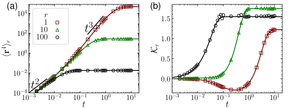
Figure 6: ABP under stochastic resetting without harmonic trap ($\beta=0$). (a) Fourth order moment of displacement $\langle{\bf r}^{4}\rangle_{r}$ (equation (81)) and (b) Kurtosis $\mathcal{K}_{r}$ as a function of time $t$ for varying resetting rates $r=1(\mathrm{squares},\Box),10(\mathrm{triangles},\triangle),100(\mathrm{circles},\circ)$ with $\mathrm{Pe}=10$. The solids lines are analytic predictions and symbols are from numerical simulations. The initial position is at the origin with the initial orientation along the $x$-axis.

Figure 6 presents the fourth-order displacement moment in (a) and the excess kurtosis in (b) as a function of time of ABP under stochastic resetting without a harmonic trap ($\beta=0$). In figure 6(a), the analytic fourth-order moment of displacement, $\langle{\bf r}^{4}\rangle_{r}$, is shown as solid lines, compared to simulation results (points) for resetting rates $r=1,~{}10,~{}100$ with $\mathrm{Pe}=10$. For low resetting rates ($r=1$), ballistic behavior $\langle{\bf r}^{4}\rangle_{r}\sim t^{3}$ is observed in the intermediate time regime. In figure 6(b), the analytic excess kurtosis, $\mathcal{K}_{r}$, is shown as solid lines, compared to simulation results (points) for the same resetting rates. Negative kurtosis is observed in the intermediate time regime for $r=1$.

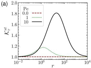
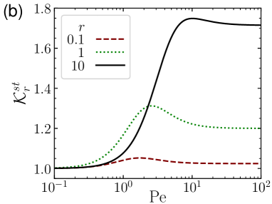
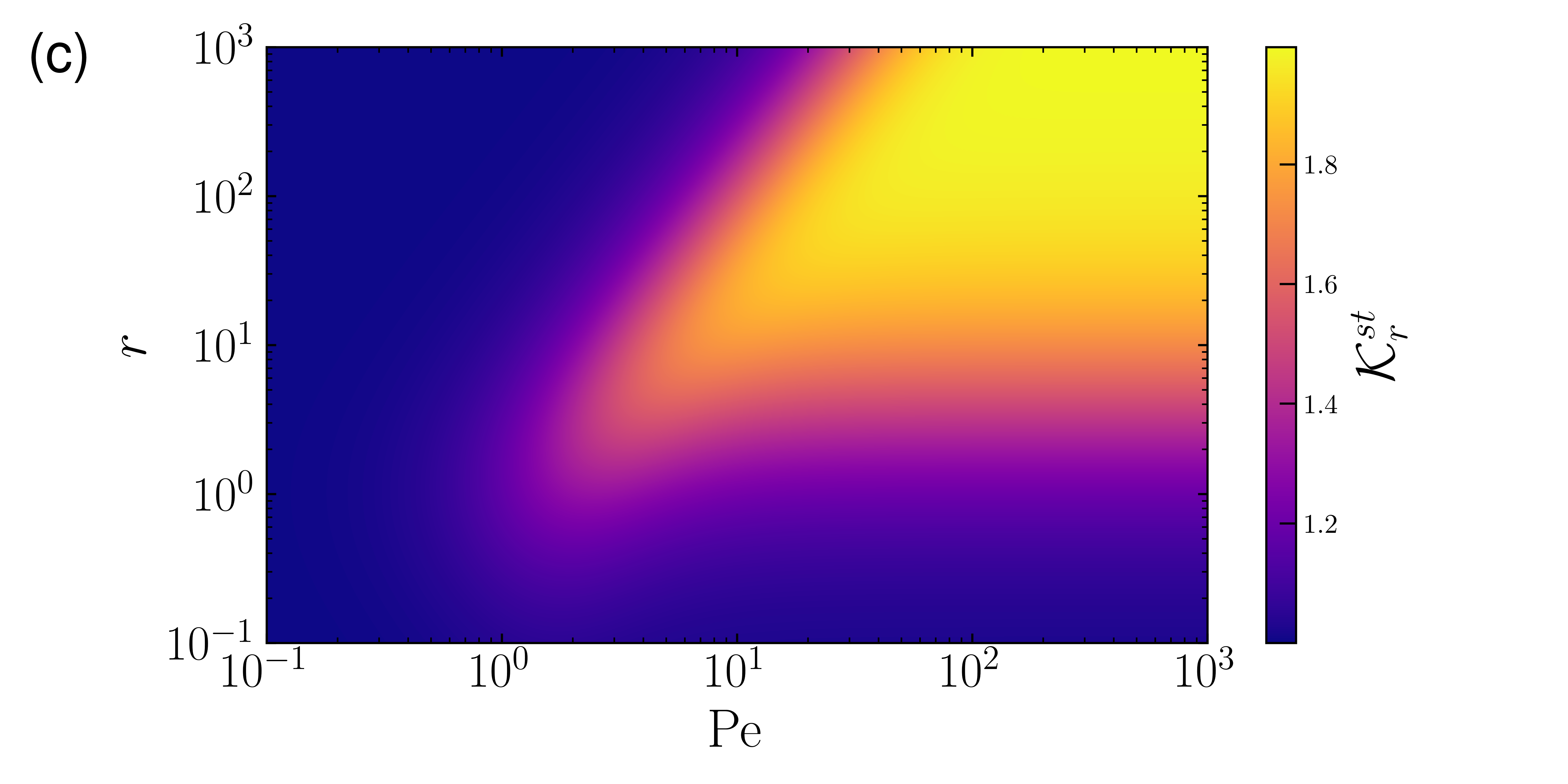
Figure 7: Steady state behavior of ABP under stochastic resetting without harmonic trap ($\beta=0$). Steady state excess kurtosis $\mathcal{K}^{st}_{r}$ (equation (22)) as a function of resetting rates ($r$) for activities $\mathrm{Pe}=0.1,~{}1,~{}10$ in (a) and as a function of $\mathrm{Pe}$ for $r=0.1,~{}1,~{}10$ in (b). (c) Plot of $\mathcal{K}^{st}_{r}$ in $r-\mathrm{Pe}$ plane.

Figure 7 presents the steady-state quantification of ABP under stochastic resetting without a harmonic trap ($\beta=0$). In figure 7(a), we show steady state kurtosis $\mathcal{K}^{st}_{r}$ (equation (22)) as a function of $r$ for $\mathrm{Pe}=0.1,~{}1,~{}10$. In figure 7(b), we show the $\mathcal{K}^{st}_{r}$ (equation (22)) as a function of $\mathrm{Pe}$ for $r=0.1,~{}1,~{}10$. We see the non-monotonic behavior of $\mathcal{K}^{st}_{r}$ as a function of $r$ with high activity $\mathrm{Pe}$ (figure 7(a)). It demonstrates the presence of an optimal resetting rate where $\mathcal{K}^{st}_{r}$ is maximized for fixed activity, suggesting a maximum heavy tail in the position distribution, which increases the likelihood of finding the particle at a very long distance. We can also observe non-monotonic in $\mathcal{K}^{st}_{r}$ as a function of $\mathrm{Pe}$ for constant $r$, which peaks at intermediate $\mathrm{Pe}$ (figure 7(b)). In figure 7(c), we show the $\mathcal{K}^{st}_{r}$ in $r-\mathrm{Pe}$ plane, exhibits this non-monotonic behavior in both parameters $r$ and $\mathrm{Pe}$.

We found that at intermediate timescales, high activity ($\mathrm{Pe}$) and low resetting rate ($r$) result in persistent behavior, characterized by bimodal distributions and negative kurtosis. At longer times, the system reaches a nonequilibrium steady state (NESS), where moments stabilize. The steady-state kurtosis shows non-monotonic behavior, deviating from the positive kurtosis value of $1$ seen in Brownian particles under resetting, across different values of both activity ($\mathrm{Pe}$) and resetting rate ($r$).

References

References

- [1] Romanczuk P, Bär M, Ebeling W, Lindner B and Schimansky-Geier L 2012 The European Physical Journal Special Topics 2012 202:1 202 1–162 ISSN 1951-6401 URL https://link.springer.com/article/10.1140/epjst/e2012-01529-y
- [2] Marchetti M C, Joanny J F, Ramaswamy S, Liverpool T B, Prost J, Rao M and Simha R A 2013 Reviews of Modern Physics 85 1143–1189 ISSN 00346861 URL https://journals.aps.org/rmp/abstract/10.1103/RevModPhys.85.1143
- [3] Cates M E and Tailleur J 2015 The Annual Review of Condensed Matter Physics is Annu. Rev. Condens. Matter Phys 6 219–244 URL www.annualreviews.org
- [4] Bechinger C, Di Leonardo R, Löwen H, Reichhardt C, Volpe G and Volpe G 2016 Reviews of Modern Physics 88 45006 URL https://link.aps.org/doi/10.1103/RevModPhys.88.045006
- [5] Ramaswamy S 2017 Journal of Statistical Mechanics: Theory and Experiment 2017 054002 ISSN 1742-5468 URL https://iopscience.iop.org/article/10.1088/1742-5468/aa6bc5
- [6] Baconnier P, Dauchot O, Démery V, Düring G, Henkes S, Huepe C and Shee A 2024 Self-aligning polar active matter arXiv:2403.10151 URL https://arxiv.org/abs/2403.10151
- [7] Schaller V, Weber C, Semmrich C, Frey E and Bausch A R 2010 Nature 467 73–77 ISSN 1476-4687 URL https://doi.org/10.1038/nature09312
- [8] Sumino Y, Nagai K H, Shitaka Y, Tanaka D, Yoshikawa K, Chaté H and Oiwa K 2012 Nature 483 448–452 ISSN 0028-0836 URL https://www.nature.com/articles/nature10874
- [9] Shee A, Gupta N, Chaudhuri A and Chaudhuri D 2021 Soft Matter 17 2120–2131 ISSN 1744-6848 URL https://pubs.rsc.org/en/content/articlehtml/2021/sm/d0sm01181ahttps://pubs.rsc.org/en/content/articlelanding/2021/sm/d0sm01181a
- [10] Karan C and Chaudhuri D 2023 Soft Matter 19 1834–1843 ISSN 1744-683X URL https://doi.org/10.1039/D2SM01183B
- [11] Ballerini M, Cabibbo N, Candelier R, Cavagna A, Cisbani E, Giardina I, Lecomte V, Orlandi A, Parisi G, Procaccini A, Viale M and Zdravkovic V 2008 Proceedings of the National Academy of Sciences 105 1232–1237 ISSN 0027-8424 URL https://pnas.org/doi/full/10.1073/pnas.0711437105
- [12] Katz Y, Tunstrøm K, Ioannou C C, Huepe C and Couzin I D 2011 Proceedings of the National Academy of Sciences 108 18720–18725 ISSN 0027-8424 URL https://pnas.org/doi/full/10.1073/pnas.1107583108
- [13] Vicsek T, Czirók A, Ben-Jacob E, Cohen I and Shochet O 1995 Physical Review Letters 75 1226–1229 URL https://link.aps.org/doi/10.1103/PhysRevLett.75.1226
- [14] Toner J, Tu Y and Ramaswamy S 2005 Annals of Physics 318 170–244 ISSN 0003-4916 URL https://www.sciencedirect.com/science/article/pii/S0003491605000540
- [15] Kumar K V, Bois J S, Jülicher F and Grill S W 2014 Physical Review Letters 112 208101 URL https://link.aps.org/doi/10.1103/PhysRevLett.112.208101
- [16] Fily Y and Marchetti M C 2012 Physical Review Letters 108 235702 URL https://link.aps.org/doi/10.1103/PhysRevLett.108.235702
- [17] Palacci J, Sacanna S, Steinberg A P, Pine D J and Chaikin P M 2013 Science 339 936–940 ISSN 10959203 URL https://www.science.org/doi/10.1126/science.1230020
- [18] Slowman A B, Evans M R and Blythe R A 2016 Phys. Rev. Lett. 116(21) 218101 URL https://link.aps.org/doi/10.1103/PhysRevLett.116.218101
- [19] Schwarz-Linek J, Valeriani C, Cacciuto A, Cates M E, Marenduzzo D, Morozov A N and Poon W C K 2012 Proceedings of the National Academy of Sciences 109 4052–4057 ISSN 0027-8424 URL https://pnas.org/doi/full/10.1073/pnas.1116334109
- [20] Bhattacherjee B and Chaudhuri D 2019 Soft Matter 15 8483–8495 ISSN 1744-683X URL https://doi.org/10.1039/C9SM00998A
- [21] Basu U, Majumdar S N, Rosso A and Schehr G 2018 Physical Review E 98 62121 URL https://link.aps.org/doi/10.1103/PhysRevE.98.062121
- [22] Shee A, Dhar A and Chaudhuri D 2020 Soft Matter 16 4776–4787 ISSN 1744-683X URL http://dx.doi.org/10.1039/D0SM00367K
- [23] Majumdar S N and Meerson B 2020 Phys. Rev. E 102(2) 022113 URL https://link.aps.org/doi/10.1103/PhysRevE.102.022113
- [24] Santra I, Basu U and Sabhapandit S 2021 Physical Review E 104 L012601 ISSN 2470-0045 URL https://link.aps.org/doi/10.1103/PhysRevE.104.L012601
- [25] Shee A and Chaudhuri D 2022 Journal of Statistical Mechanics: Theory and Experiment 2022 013201 ISSN 1742-5468 URL https://iopscience.iop.org/article/10.1088/1742-5468/ac403f
- [26] Patel M and Chaudhuri D 2023 New Journal of Physics 25 123048 ISSN 1367-2630 URL https://iopscience.iop.org/article/10.1088/1367-2630/ad1538
- [27] Pototsky A and Stark H 2012 EPL (Europhysics Letters) 98 50004 ISSN 0295-5075 URL https://iopscience.iop.org/article/10.1209/0295-5075/98/50004
- [28] Solon A P, Cates M E and Tailleur J 2015 The European Physical Journal Special Topics 224 1231–1262 ISSN 1951-6355 URL http://link.springer.com/10.1140/epjst/e2015-02457-0
- [29] Malakar K, Das A, Kundu A, Kumar K V and Dhar A 2020 Physical Review E 101 022610 ISSN 2470-0045 URL https://link.aps.org/doi/10.1103/PhysRevE.101.022610
- [30] Chaudhuri D and Dhar A 2021 Journal of Statistical Mechanics: Theory and Experiment 2021 013207 URL https://dx.doi.org/10.1088/1742-5468/abd031
- [31] Malakar K, Jemseena V, Kundu A, Vijay Kumar K, Sabhapandit S, Majumdar S N, Redner S and Dhar A 2018 Journal of Statistical Mechanics: Theory and Experiment 2018 043215 ISSN 1742-5468 URL https://iopscience.iop.org/article/10.1088/1742-5468/aab84f
- [32] Basu U, Majumdar S N, Rosso A and Schehr G 2019 Physical Review E 100 062116 ISSN 2470-0045 URL https://link.aps.org/doi/10.1103/PhysRevE.100.062116
- [33] Dhar A, Kundu A, Majumdar S N, Sabhapandit S and Schehr G 2019 Physical Review E 99 032132 ISSN 2470-0045 URL https://link.aps.org/doi/10.1103/PhysRevE.99.032132
- [34] Singh P and Kundu A 2019 Journal of Statistical Mechanics: Theory and Experiment 2019 083205 ISSN 1742-5468 URL http://arxiv.org/abs/1906.09442http://dx.doi.org/10.1088/1742-5468/ab3283
- [35] Fernandez-Rodriguez M A, Grillo F, Alvarez L, Rathlef M, Buttinoni I, Volpe G and Isa L 2020 Nature Communications 11 4223 ISSN 2041-1723 URL https://www.nature.com/articles/s41467-020-17864-4
- [36] Beppu K and Timonen J V I 2024 Communications Physics 7 216 ISSN 2399-3650 URL https://www.nature.com/articles/s42005-024-01707-5
- [37] Ziepke A, Maryshev I, Aranson I S and Frey E 2022 Nature Communications 13 6727 ISSN 2041-1723 URL https://www.nature.com/articles/s41467-022-34484-2
- [38] Deng Y, Paskert A, Zhang Z, Wittkowski R and Ahmed D 2023 Science Advances 9 eadh5260 ISSN 2375-2548 URL https://www.science.org/doi/10.1126/sciadv.adh5260
- [39] Zhang Z, Allegrini L K, Yanagisawa N, Deng Y, Neuhauss S C F and Ahmed D 2023 IEEE Robotics and Automation Letters 8 2598–2605 ISSN 2377-3766 URL https://ieeexplore.ieee.org/document/10073566/
- [40] Evans M R and Majumdar S N 2011 Phys. Rev. Lett. 106(16) 160601 URL https://link.aps.org/doi/10.1103/PhysRevLett.106.160601
- [41] Evans M R and Majumdar S N 2011 Journal of Physics A: Mathematical and Theoretical 44 435001 ISSN 1751-8113 URL https://iopscience.iop.org/article/10.1088/1751-8113/44/43/435001
- [42] Reuveni S 2016 Phys. Rev. Lett. 116(17) 170601 URL https://link.aps.org/doi/10.1103/PhysRevLett.116.170601
- [43] Majumdar S N, Sabhapandit S and Schehr G 2015 Phys. Rev. E 91(5) 052131 URL https://link.aps.org/doi/10.1103/PhysRevE.91.052131
- [44] Pal A and Reuveni S 2017 Phys. Rev. Lett. 118(3) 030603 URL https://link.aps.org/doi/10.1103/PhysRevLett.118.030603
- [45] Manrubia S C and Zanette D H 1999 Phys. Rev. E 59(5) 4945–4948 URL https://link.aps.org/doi/10.1103/PhysRevE.59.4945
- [46] Montanari A and Zecchina R 2002 Phys. Rev. Lett. 88(17) 178701 URL https://link.aps.org/doi/10.1103/PhysRevLett.88.178701
- [47] Kussell E and Leibler S 2005 Science 309 2075–2078 ISSN 0036-8075 URL https://www.science.org/doi/10.1126/science.1114383
- [48] Kussell E, Kishony R, Balaban N Q and Leibler S 2005 Genetics 169 1807–14 ISSN 0016-6731 URL https://doi.org/10.1534/genetics.104.035352
- [49] Visco P, Allen R J, Majumdar S N and Evans M R 2010 Biophysical Journal 98 1099–1108 ISSN 00063495 URL https://linkinghub.elsevier.com/retrieve/pii/S0006349509060998
- [50] Roldán E, Lisica A, Sánchez-Taltavull D and Grill S W 2016 Phys. Rev. E 93(6) 062411 URL https://link.aps.org/doi/10.1103/PhysRevE.93.062411
- [51] Evans M R, Majumdar S N and Schehr G 2020 Journal of Physics A: Mathematical and Theoretical 53 193001 ISSN 1751-8113 URL https://iopscience.iop.org/article/10.1088/1751-8121/ab7cfe
- [52] Pal A, Kostinski S and Reuveni S 2022 Journal of Physics A: Mathematical and Theoretical 55 021001 ISSN 1751-8113 URL https://iopscience.iop.org/article/10.1088/1751-8121/ac3cdf
- [53] Evans M R, Majumdar S N and Mallick K 2013 Journal of Physics A: Mathematical and Theoretical 46 185001 ISSN 1751-8113 URL https://iopscience.iop.org/article/10.1088/1751-8113/46/18/185001
- [54] Whitehouse J, Evans M R and Majumdar S N 2013 Phys. Rev. E 87(2) 022118 URL https://link.aps.org/doi/10.1103/PhysRevE.87.022118
- [55] Evans M R and Majumdar S N 2014 Journal of Physics A: Mathematical and Theoretical 47 285001 ISSN 1751-8113 URL https://iopscience.iop.org/article/10.1088/1751-8113/47/28/285001
- [56] Pal A 2015 Phys. Rev. E 91(1) 012113 URL https://link.aps.org/doi/10.1103/PhysRevE.91.012113
- [57] Méndez V m c and Campos D 2016 Phys. Rev. E 93(2) 022106 URL https://link.aps.org/doi/10.1103/PhysRevE.93.022106
- [58] Masó-Puigdellosas A, Campos D and Méndez V m c 2019 Phys. Rev. E 99(1) 012141 URL https://link.aps.org/doi/10.1103/PhysRevE.99.012141
- [59] Pal A, Chatterjee R, Reuveni S and Kundu A 2019 Journal of Physics A: Mathematical and Theoretical 52 264002 ISSN 1751-8113 URL http://arxiv.org/abs/1902.00907http://dx.doi.org/10.1088/1751-8121/ab2069
- [60] Gupta D 2019 Journal of Statistical Mechanics: Theory and Experiment 2019 033212 ISSN 1742-5468 URL https://iopscience.iop.org/article/10.1088/1742-5468/ab054a
- [61] Ahmad S, Nayak I, Bansal A, Nandi A and Das D 2019 Phys. Rev. E 99(2) 022130 URL https://link.aps.org/doi/10.1103/PhysRevE.99.022130
- [62] Tal-Friedman O, Pal A, Sekhon A, Reuveni S and Roichman Y 2020 The Journal of Physical Chemistry Letters 11 7350–7355 ISSN 1948-7185 URL https://pubs.acs.org/doi/10.1021/acs.jpclett.0c02122
- [63] Singh P 2020 Journal of Physics A: Mathematical and Theoretical 53 405005 ISSN 1751-8113 URL http://arxiv.org/abs/2007.05576http://dx.doi.org/10.1088/1751-8121/abaf2d
- [64] Mercado-Vásquez G, Boyer D, Majumdar S N and Schehr G 2020 Journal of Statistical Mechanics: Theory and Experiment 2020 113203 ISSN 1742-5468 URL https://iopscience.iop.org/article/10.1088/1742-5468/abc1d9
- [65] Ray S and Reuveni S 2020 The Journal of Chemical Physics 152 234110 ISSN 0021-9606 URL https://pubs.aip.org/jcp/article/152/23/234110/947296/Diffusion-with-resetting-in-a-logarithmic
- [66] Kumar V, Sadekar O and Basu U 2020 Phys. Rev. E 102(5) 052129 URL https://link.aps.org/doi/10.1103/PhysRevE.102.052129
- [67] Sar G K, Ray A, Ghosh D, Hens C and Pal A 2023 Soft Matter 19 4502–4518 ISSN 1744-683X URL https://doi.org/10.1039/D3SM00271C
- [68] Abdoli I and Sharma A 2021 Soft Matter 17 1307–1316 ISSN 1744-683X URL https://doi.org/10.1039/D0SM01773F
- [69] Zhang W, Li Y, Marchesoni F, Misko V R and Ghosh P K 2023 Entropy 25 271 ISSN 1099-4300 URL https://www.mdpi.com/1099-4300/25/2/271
- [70] Guéneau M, Majumdar S N and Schehr G 2024 Europhysics Letters 145 61002 ISSN 0295-5075 URL https://iopscience.iop.org/article/10.1209/0295-5075/ad2ba3
- [71] Evans M R and Majumdar S N 2018 Journal of Physics A: Mathematical and Theoretical 51 475003 URL https://dx.doi.org/10.1088/1751-8121/aae74e
- [72] Bressloff P C 2020 Journal of Physics A: Mathematical and Theoretical 53 425001 URL https://dx.doi.org/10.1088/1751-8121/abb844
- [73] Schumm R D and Bressloff P C 2021 Journal of Physics A: Mathematical and Theoretical 54 404004 ISSN 1751-8113 URL https://iopscience.iop.org/article/10.1088/1751-8121/ac219b
- [74] Baouche Y, Franosch T, Meiners M and Kurzthaler C 2024 New Journal of Physics 26 073041 ISSN 1367-2630 URL https://iopscience.iop.org/article/10.1088/1367-2630/ad602a
- [75] Hermans J and Ullman R 1952 Physica 18 951–971 ISSN 00318914 URL https://linkinghub.elsevier.com/retrieve/pii/S0031891452802319
- [76] Shee A and Chaudhuri D 2022 Physical Review E 105 54148 URL https://link.aps.org/doi/10.1103/PhysRevE.105.054148
- [77] Pattanayak A, Shee A, Chaudhuri D and Chaudhuri A 2024 New Journal of Physics ISSN 1367-2630 URL https://iopscience.iop.org/article/10.1088/1367-2630/ad6a32
- [78] Patel M and Chaudhuri D 2024 New Journal of Physics 26 073048 ISSN 1367-2630 URL https://iopscience.iop.org/article/10.1088/1367-2630/ad6349
- [79] Paramanick S, Biswas A, Soni H, Pal A and Kumar N 2024 PRX Life 2(3) 033007 URL https://link.aps.org/doi/10.1103/PRXLife.2.033007