Scalable Multivariate Fronthaul Quantization for Cell-Free Massive MIMO
Abstract
The conventional approach to the fronthaul design for cell-free massive MIMO system follows the compress-and-precode (CP) paradigm. Accordingly, encoded bits and precoding coefficients are shared by the distributed unit (DU) on the fronthaul links, and precoding takes place at the radio units (RUs). Previous theoretical work has shown that CP can be potentially improved by a significant margin by precode-and-compress (PC) methods, in which all baseband processing is carried out at the DU, which compresses the precoded signals for transmission on the fronthaul links. The theoretical performance gain of PC methods are particularly pronounced when the DU implements multivariate quantization (MQ), applying joint quantization across the signals for all the RUs. However, existing solutions for MQ are characterized by a computational complexity that grows exponentially with the sum-fronthaul capacity from the DU to all RUs. This work sets out to design scalable MQ strategies for PC-based cell-free massive MIMO systems. For the low-fronthaul capacity regime, we present -parallel MQ (-PMQ), whose complexity is exponential only in the fronthaul capacity towards an individual RU, while performing close to full MQ. -PMQ tailors MQ to the topology of the network by allowing for parallel local quantization steps for RUs that do not interfere too much with each other. For the high-fronthaul capacity regime, we then introduce neural MQ, which replaces the exhaustive search in MQ with gradient-based updates for a neural-network-based decoder, attaining a complexity that grows linearly with the sum-fronthaul capacity. Numerical results demonstrate that the proposed scalable MQ strategies outperform CP for both the low and high-fronthaul capacity regimes at the cost of increased computational complexity at the DU (but not at the RUs).
I Introduction
I-A Context and Motivation
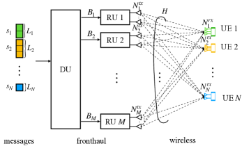
In modern wireless systems, base stations are disaggregated into radio units (RUs), distributed units (DUs), and central units (CUs), with RUs and DUs connected via fronthaul links. As shown in Fig. 1, a DU may control several RUs, supporting coordinated transmission and reception across multiple distributed RUs [1, 2]. While several functional splits between DUs and RUs have been defined, current deployments adopt a specific split, typically referred to as 7.2x, whereby lower-physical layer (PHY) functionalities such as precoding are carried out closer to the antennas, at the RU, while higher-PHY functionalities such as encoding are implemented at the DU [3, 4]. This functional split becomes problematic for regimes characterized by massive antenna arrays and large spectral efficiencies [3]. This issue is currently one of the key factors limiting the deployment of cell-free massive MIMO systems based on disaggregated base stations, such as O-RAN [5, 2].
In the downlink, the 7.2x functional split prescribes an approach that may be referred to as compress-and-precode (CP). As shown in Fig. 2 (left), with CP, the DU applies channel coding to all the information bits, and evaluates the precoding matrices, which are transmitted in a compressed form to every RU via the corresponding fronthaul link. Hence, the fronthaul overhead of this approach may be substantial due to the separate transmission of precoding matrices and coded bits.
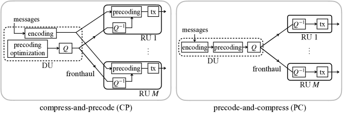
To mitigate this problem, an alternative functional split has been introduced in which the DU applies coding and precoding, transmitting to each RU the respective complex baseband signals after compression [6, 7, 8]. This way, as suggested by the theoretical results in [6, 9, 1], the fronthaul capacity requirements may be drastically reduced. We refer to such an approach as precode-and-compress (PC), which is the subject of this paper and is illustrated in Fig. 2 (right).
While the PC functional split has the potential to effectively lessen the fronthaul capacity, the theoretical results in [6] require complex baseband compression schemes at the DU, whose practical implementation is an open problem. Some steps in this direction were reported in [7], which proposes multivariate quantization (MQ), whereby the baseband signals for all RUs are quantized jointly [7].
Specifically, reference [7] proposed a data-driven algorithm for MQ that was shown to outperform existing per-RU point-to-point quantization techniques. However, the algorithm in [7] suffers from a computational complexity that grows exponentially in the fronthaul sum-rate, and is also limited to the case in which all the UEs and RUs are equipped with single antennas. The goal of this paper is to design practical, scalable PC-based solutions for distributed large-scale MIMO systems.
I-B Related Work
Recent work on fronthaul design for cell-free massive MIMO has aimed at (i) enhancing CP; (ii) improving PC; and (iii) proposing hybrid methods between CP and PC, corresponding different functional splits.
Representative papers on CP include [10], which addresses precoder design by taking into account the limited fronthaul capacity; as well as [11, 12], which consider optimizing the allocation of resources. Recent advances in PC have focused on linear dimension reduction techniques [13, 14, 8] followed by uniform quantization. These schemes require sharing the linear transformation matrix, which entails additional fronthaul communication overhead, which may become substantial in cell-free massive MIMO systems. This limitation has been recently alleviated via meta-learning [8].
Lastly, alternatives to CP and PC have been studied [15, 16, 17] that showcase the optimality of different functional splits depending on the underlying dynamics of the system. These schemes require the solution of non-convex optimization problems or lower-complexity methods such as reinforcement learning [17].
I-C Main Contribution
This work introduces two new MQ techniques for PC-based transmission in cell-free massive MIMO systems. The main contributions of this work can be summarized as follows:
-
•
We introduce -parallel multivariate quantization (-PMQ), a novel MQ scheme that has computational complexity growing exponentially only in the per-RU fronthaul rate, while demonstrating a small performance gap with respect to MQ [7] in the low-fronthaul capacity regime. -PMQ tailors MQ to the topology of the network by allowing for parallel local quantization steps for RUs that do not interfere too much with each other.
-
•
Furthermore, we introduce neural-multivariate quantization (neural-MQ), another novel MQ scheme with computational complexity that grows linearly in the fronthaul sum-rate. Neural-MQ replaces the exhaustive search in MQ with gradient-based updates for a neural-network-based decoder. We demonstrate that neural-MQ outperforms CP, as well as an infinite precoding benchmark that assumes linear precoding, in the high-fronthaul capacity regime.
The rest of the paper is organized as follows. In Sec. II, we describe the general system model of the cell-free MIMO systems, and review the state-of-the-art PC-based solution [7] designed for single-antenna UEs and RUs in Sec. III. We then propose -PMQ in Sec. IV and neural-MQ in Sec. V. Experimental results are provided in Sec. VI, and Sec. VII concludes the paper.
II System Model
II-A Setting
As shown in Fig. 1, in the cell-free setting of interest, a set of RUs communicates to UEs through RUs. The -th RU has transmit antennas, and is connected to the DU through a fronthaul link with capacity bits per channel use, i.e., the fronthaul link carries bit/s/Hz when normalized by the bandwidth of the radio interface. Each -th UE has antennas. We denote the overall number of transmit antennas as , i.e., , and the overall number of receive antennas as .
The DU wishes to transmit an vector of complex symbols to each -th UE for on each channel use . The information symbols are assumed to be zero mean and independent, and we normalize their powers such that the equality holds for all , where is the identity matrix.
Denote as the channel matrix between all RUs and UE for channel use , and as
| (1) |
the overall channel matrix of size . The precoding matrix
| (2) |
collects all the precoding matrices used to precode symbols towards user for for channel use . The precoding matrices are optimized by the DU based on knowledge of the channel matrices .
Given the precoding matrix for channel use , and further denoting as the precoding matrix used by RU to communicate with UE which gives the overall precoding matrix for user , the precoded symbol vector is given by
| (3) |
as a function of the symbol vector . We partition the precoded vector in (3) across the RUs as
| (4) |
where
| (5) |
denoting as the precoding matrix associated to RU . Note the slight abuse of notation, as represents the beamforming matrix for UE and the beamforming matrix for RU .
Due to fronthaul capacity limitations, as we will detail in the rest of the section, the symbol vector transmitted by RU at channel use , denoted as , may differ from the precoded vector in (4). We impose the average power constraint
| (6) |
for each RU , where the expectation is taken with respect to transmit symbols . Given the transmit vector for all , the received signal vector at the UE is given by
| (7) |
where is the complex Gaussian noise vector.
Given an receive beamforming matrix , UE estimates the transmitted signal at channel use as
| (8) |
for all . The receive beamforming matrix is generally designed by UE based on the available channel state information. We will address this point in Sec. V-C.
II-B Compress-and-Precode
In the conventional compress-and-precode (CP) strategy, the DU applies an entry-wise uniform quantizer to the precoding matrix for each RU , producing the quantized precoding matrix
| (9) |
The quantizer has a resolution of bits per entry. The DU then sends the bits describing the quantized matrix to RU on the fronthaul along with the information bits for all UEs to the -th RU on the fronthaul. Each -th RU then transmits the signal
| (10) |
where is a parameter introduced to satisfy the power constraint (6).
While precoding matrix is in principle designed per-channel-use basis, in order to reduce the fronthaul overhead, CP typically shares the same precoding matrix across multiple channel uses[20, 4]. Increasing generally entails a trade-off between quality of precoding, which increases with a smaller , and fronthaul overhead, which decreases as grows larger. In fact, the fronthaul capacity constraint imposes the inequality
| (11) |
where is the sum-rate, in bits per channel use, across all UEs, and is the channel coding rate. The first term, , in (11) accounts for the transmission of all coded bits to each RU, while the second term accounts for precoding information.
II-C Precode-and-Compress
Unlike CP strategies, PC methods [6, 7] compress directly the precoded vector (3). As a result, the quantized vector is given by
| (12) |
for some quantization function with resolution bits. Note that function may apply jointly across all entries of the vector [7]. We denote as the discrete index identifying the quantized signal transmitted by DU to RU on the fronthaul link at channel use .
The mapping between bits and baseband symbols , which is to be applied by RU , is defined by an inverse quantization function
| (13) |
We will further denote as the collection of the quantized outputs for all RUs, i.e., with .
After recovering the dequantized vector from the bits , the RU transmits the vector
| (14) |
in which we denote as the quantized precoded symbol transmitted at the -th antenna of RU at channel use , and the parameter ensures the power constraint (6) as for CP in (10). Combining the signals transmitted by all RUs, we can write (14) as
| (15) |
where with being the all-one vector of size .
II-D Precode-and-Compress with Conventional Quantization
In this subsection, we introduce a benchmark transmission scheme based on PC method and conventional vector quantization (VQ) [7]. Throughout the rest of the paper, we omit the channel use index to simplify the notation. Conventional VQ is applied in a point-to-point manner, separately for each RU, yielding a quantized vector for each precoded signal for RU .
To this end, let us fix a quantization codebook containing vectors of size , as well as an arbitrary mapping between bits and codewords in set . VQ finds the quantized vector for each RU as
| (16) |
and we denote as
| (17) |
The vectors in the codebook can be ideally optimized for each RU by addressing the problem of minimizing the average quantization error, i.e., [7]
| (18) |
where the average is taken over both symbols and channels .
In practice, the quantization codebook is shared across many coherence intervals, and is updated only when the channel statistics change significantly. Therefore, the codebook is modified only occasionally, and need not be accounted for when evaluating the fronthaul overhead of PC.
III State of the Art on Multivariate Quantization
This section summarizes the state-of-the-art fronthaul multivariate quantization (MQ) schemes introduced in [7] for PC. Reference [7] assumed single-antenna RUs, i.e., , single-antenna UEs, i.e., , and a single message per UE, i.e., , and it focused on a single channel use. Accordingly, in this section, we set for all , and we drop the channel use superscript . Furthermore, since the receive beamforming matrix in (8) reduces to a scalar gain, we set it without loss of generality to . Finally, reference [7] assumed an average power constraint over both channels and transmitted symbols , which is less strict than the per-channel average power constraint (6), and thus here we modify the MQ scheme in [7] to satisfy the constraint (6).
III-A Multivariate Quantization
Given a fronthaul capacity for the -th RU, the quantization codebook contains quantization codewords, i.e., (see Sec. II-D), which represent the possible values of the quantized signals (14) transmitted by RU . Each codeword is indexed by bits . We further denote as the collection of codebooks for all RUs. MQ [7] implements a quantization function in (12) that selects the codeword index to transmit through the fronthaul link to each RU via an exhaustive search over the combination of codewords.
Specifically, MQ implements the quantization function
| (19) |
and we denote as
| (20) |
where is the effective interference (EI) caused by the choice of codewords on UE . The EI criterion will be introduced in the next subsection.
III-B Effective Interference
To complete the description of the MQ rule in (19), we now introduce the EI objective function [7]. To this end, we write the average effective SINR for UE as
| (21) |
where stands for the variance of the complex Gaussian noise at the UEs and we have used (15). The numerator in (21) represents the average power of the useful part of the received signal, , assuming no quantization, while the denominator in the sum of the noise power, , and of the EI.
The EI for UE is the power of the quantization error and of the interference affecting reception at UE . From (21), the EI can be expressed as
| (22) |
The notation makes explicit the dependence of the EI for each UE on the quantized signal .
III-C Sequential Multivariate Quantization
As mentioned, problem (19) requires an exhaustive search over a space that is exponentially large in the sum-fronthaul rate , i.e., the complexity is of the order (see Table I). To address this computational complexity issue, inspired by the information-theoretic optimality of sequential encoding in the regime of infinitely long blocklengths, reference [7] proposed a sequential MQ (SMQ) scheme.
With SMQ, the DU applies local quantization for the signals to be sent to each RU on the fronthaul by searching only over the respective codebooks of the RUs. This search is done sequentially, one RU at a time, by following an arbitrary order over the RUs. Furthermore, quantization for each RU takes into account the outputs of the local quantization steps for the previously considered RUs in the given order.
Mathematically, assuming for illustration the order , over the RU index , SMQ obtains the -th component of the quantized signal as
| (23) |
and we denote as
| (24) |
with containing the quantized signals for the previously considered RUs. Accordingly, the signal for RU is obtained by fixing the quantized signals for the previously considered RUs, while setting the other transmitted signals to zero. After addressing problem (23) sequentially for all RUs, the quantized vector is obtained as as in (12).
The complexity of SMQ is linear in the number of RUs, scaling as , since each problem (23) requires a search over the codewords in codebook (see Table I).
| PC scheme | computational complexity |
|---|---|
| VQ | |
| MQ | |
| SMQ | |
| -PMQ | |
| neural-MQ |
III-D Codebook Optimization
In order to design the codebooks , reference [7] used a data-driven algorithm, namely Lloyd-Max, also known as -means [21], that alternates between solving convex problems and addressing the exponential-complexity MQ problem (19).
IV -Parallel Mutlivariate Quantization
As discussed in Sec. III-C, SMQ reduces the computational complexity of MQ via sequential local quantization steps at the RUs for a number of iterations equal to the number of RUs. However, this approach was shown in [7] to have a significant performance gap as compared to MQ.
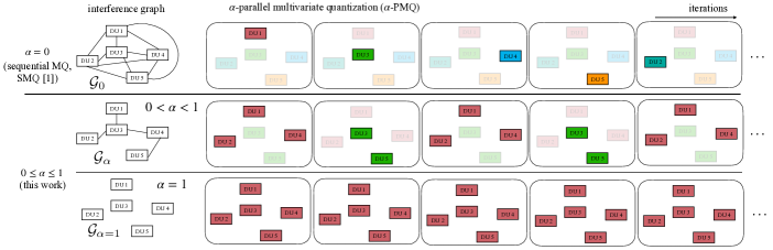
In this section, we generalize SMQ by proposing -parallel multivariate quantization (-PMQ), which shares with SMQ the complexity of order for quantization (see Table I), while significantly reducing the performance gap with respect to MQ. As illustrated in Fig. 3, the main idea of -PMQ is to allow for parallel local quantization steps at RUs that do not interfere too much with each other. Accordingly, -PMQ is tailored to the topology of the network. We continue to focus on the single antenna case in order to maintain consistency with [7], while the extension to multiple antenna case will be discussed in Sec. V-E.
IV-A EI Decomposition
We start by rewriting the EI in (22) by isolating the separate contribution of all RUs. Specifically, we write
| (26) |
where the scalar represents the disturbance from RU to UE ; is the channel between RU and UE ; and is the precoding used by RU to communicate to UE . With definition (26), the sum-EI criterion for MQ in (19) can be equivalently rewritten as
| (27) |
where we have denoted for the disturbance vector from RU to all UEs.
IV-B -Parallel Multivariate Quantization
As illustrated in Fig. 3, -PMQ operates sequentially like SMQ. However, unlike SMQ, at each iteration, rather than evaluating the quantized signal for a single RU, -PMQ applies parallel local quantization steps for a suitably chosen subset of RUs. In this regard, SMQ can be viewed as a special case of -PMQ in which only one RU applies local quantization at each iteration.
Let us define as the subset of RUs for which the DU updates the quantized signals at iteration . How to construct the sequence of these subsets will be discussed in the next subsection. At each iteration , for each RU , the DU chooses a quantized symbol , while for all RUs it sets . All quantized signals are initialized to be equal to zero. Given the updated quantized signals, for all RUs , the disturbance vector is updated accordingly using definition (26), as
| (28) |
For all RUs , the DU sets .
We now discuss how to update the quantized signals at any iteration . Given the disturbance vector from the previous iteration, and subset , -PMQ solves in parallel the problems
| (29) |
and we denote as
| (30) |
for all RUs , where we have defined as
| (31) |
the disturbance from RUs other than , along with
| (32) |
where as defined in (26). Problem (29) is a modified version of the original objective of MQ in (19) in which the contributions to the EI from all RUs other than are fixed to the values obtained at the previous iteration. One can directly check that by setting and , -PMQ recovers SMQ.
IV-C Optimizing the Update Schedule
The main idea behind the selection of subsets is to allow for parallel local quantization steps (29) only for RUs that do not interfere too much with each other. The intuition is that RUs whose transmitted signals affect significantly the same subset of devices should be optimized jointly, which is facilitated by sequential, rather than parallel, optimization.
To elaborate, let us define the channel gain vector for node as
| (33) |
Then, we build an interference graph by defining the edge set as
| (34) |
with the threshold defined to ensure that the number of the edges is a fraction of the total number of edges , i.e., , with ceiling operation . Mathematically, the threshold is defined as
| (35) |
denoting as the -th smallest value in the set with . For the interference graph is disconnected, while for , it becomes fully connected.
Given the interference graph, -PMQ seeks for subsets of nodes that are not connected by edges, indicating that the corresponding RUs do not interference to much with each other. To this end, the algorithm obtains independent sets . By definition, an independent set is such that for any , there is no edge in the interference graph, i.e., . We follow the recursive largest first (RLF) algorithm [22] to find the independent sets from the interference graph . We choose as the -th independent set, where is the number of independent sets returned by RLF. Overall procedure of -PMQ is summarized in Algorithm 1.
IV-D Codebook Optimization with -PMQ
V Neural Multivariate Quantization
All schemes presented so far require exhaustive searches over discrete spaces of cardinality growing exponentially with the fronthaul capacity. While this is feasible when the fronthaul capacity are, say, up to – bits per channel use, it becomes quickly impractical for larger values of the fronthaul capacity . In this section, we introduce neural-network-based multivariate quantization, referred to as neural multivariate quantization (neural-MQ), which replaces exhaustive search with gradient-based updates with the aid of a neural-network-based decoder. The approach is presented for general multi-antenna systems, and a modification of the EI criterion to this setting is also introduced in this section.
V-A Neural Multivariate Quantization
Instead of solving a discrete optimization problem of complexity like MQ, neural-MQ relaxes the search space to the vector space , enabling the use of gradient-based updates. This approach is used also in the literature on combinatorial optimization [23, 24]. Following [24], we also incorporate an annealing mechanism to mitigate the distinction caused by the relaxation.
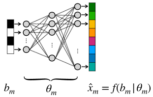
Specifically, as shown in Fig. 4, neural-MQ introduces a neural network, or neural codebook, , parameterized by a vector that determines the synaptic weights and biases of the neural network [21], that takes as an input the binary message for RU and outputs the corresponding signal for each RU . Note that in the previous sections, the function was implemented by a look-up table that recovers the quantized signal given the index .
Accordingly, quantization is carried out, as in (19), by addressing the problem
| (36) |
from which we have the overall quantized vector
| (37) |
given .
To address the combinatorial problem (36), we relax the problem by considering the optimization
| (38) |
over the real-valued vector , where we have defined the sigmoid function with temperature as [21]
| (39) |
which is applied element-wise in (38). The sigmoid function (39) squashes (unconstrained) real number into an interval . As the temperature decreases, the sigmoid function becomes increasingly close to a hard step function.
Accordingly, given an optimized real vector , the final solution is obtained as
| (40) |
which can then be transmitted to each RU via the fronthaul link of capacity . After receiving , each RU can transmit the signal by simply running the neural network once, i.e., computing and transmitting with power scaling factor .
Problem (38) is addressed via gradient descent (GD) with temperature annealing [24]. Thus, we decrease temperature by setting the temperature at -th GD step as for a given total number of GD updates. The overall procedure of neural-MQ is summarized in Algorithm 2.
The computational complexity of neural-MQ is determined by the number of GD updates as well as the number of (hidden) neurons in the neural network . For instance if one adopts as a fully-connected neural network with hidden layers each with neurons, solving (36) via (38) would require computational complexity of the order [21, 25] which grows linearly with fronthaul sum-rate at the DU side, while at the RU side, it requires for each RU (see Table I).
V-B Multi-Antenna Effective Interference
As explained in the previous section, the EI criterion (22) studied in [7] and reviewed in Sec. III assumes single-antenna for both RUs and UEs. In this subsection, we extend, and modify, the notion of EI to the scenario presented in Sec. II in which both RUs and UEs are equipped with multiple antennas. As in the previous section, we simplify the notation by removing the explicit dependence on the channel use index .
Accounting for the effect of the beamforming receiver matrix, the expected discrepancy between the desired symbol and the estimated symbol can be characterized by the error covariance matrix (see, e.g., [26])
| (41) |
where the expectation is taken with respect to the random symbol as well as the noise vector in (7). We propose to use as EI criterion the trace of the error covariance matrix, which can be simplified as follows by retaining only the terms that depend on the quantization process
| (42) |
Note that the precoded signal appears implicitly in (42), as for the original EI (22), through its individual precoded signals. In particular, the EI criterion (42) recovers (22) by setting .
V-C Receive Beamforming
The EI criterion (42) is defined for any receive beamforming matrix . For instance, MMSE receiver can be adopted [27]
| (43) |
which requires the availability of all the effective channels , that is, of its own effective channel as well as of the effective channels for all the other UEs . A more practical approach would be to adopt a localized MMSE receiver, which can be justified by the channel hardening effect of cell-free massive MIMO (see, e.g., [2, 28]), i.e.,
| (44) |
V-D Neural Codebook Optimization
V-E Extending -PMQ to Multi-Antenna Systems
As a final note, using (42), it is straightforward to extend -PMQ, presented in Sec. IV, to multi-antenna systems by noting that EI in (42) can be also decomposed into the terms that explicitly shows the dependence on each RU . This can be done as
| (46) |
denoting as and the beamforming matrix of UE designed for RU and the channel matrix between UE and RU , respectively.
| (47) | ||||
VI Experimental Results111Code is available at https://github.com/kclip/scalable-MQ.
In this section, we investigate the scalability of the proposed PC-based solutions by separating the analysis into low-fronthaul and high-fronthaul regimes. In the low fronthaul regime, we compare the proposed -PMQ (Sec. IV) and neural-MQ (Sec. V) against conventional PC schemes, i.e., VQ (Sec. II-D) [7], SMQ (Sec. III-C), and MQ (Sec. III-A). We specifically focus on a regime with a low fronthaul capacity, in which CP cannot be evaluated even under the minimum scalar quantization level with maximum precoding sharing factor [4].
In the high-fronthaul regime, we focus on comparing neural-MQ with CP, since all the other PC-based solutions, including -PMQ, cannot be run in a reasonable time due to their exponential complexity. In this regime, we consider instead two infinite-fronthaul benchmarks. The first stipulates that the RUs transmit directly the linearly precoded vector .
In the second, we address problem (38) by optimizing the transmitted signal as , where is an arbitrary complex-valued vector. This solution can be considered to be a type of non-linear precoding, which may outperform linear precoding [29]. Being based on optimization (38), the performance of the proposed neural-MQ scheme is upper bounded by the second, non-linear, infinite-fronthaul benchmark scheme, but not by the first, linear precoding, benchmark.
For all the experiments, we set the total signal-to-noise ratio (SNR) as dB, unless specified otherwise; and we assume the same power for all the RUs. Codebook optimization for both -PMQ (Sec. IV-D) and neural-MQ (Sec. V-D) is done by assuming Gaussian information symbols using different channel realizations and different Gaussian symbols. Specifically, we use CVX [30] for codebook optimization of -PMQ, while the Adam optimizer [31] is adopted for codebook optimization of neural-MQ.
The performance of the PC-based solutions are evaluated based on the sum-spectral efficiency and the symbol error rate. The sum-spectral efficiency is evaluated as , where the expectation over symbols is estimated by Gaussian symbols, while the expectation over channels is estimated by five different channel realizations following 3GPP urban micro (UMi) channel models [32]. When evaluating symbol error rate, we consider 16 quadrature amplitude modulation (16-QAM) symbols, and report the average symbol error rate over the UEs.
Lastly, we adopt MMSE precoding and localized MMSE receive beamforming (44). For neural-MQ, we set the number of GD steps , number of hidden layers , and the number of hidden neurons , unless specified otherwise.
VI-A Low-Fronthaul Capacity: Computational Complexity Analysis
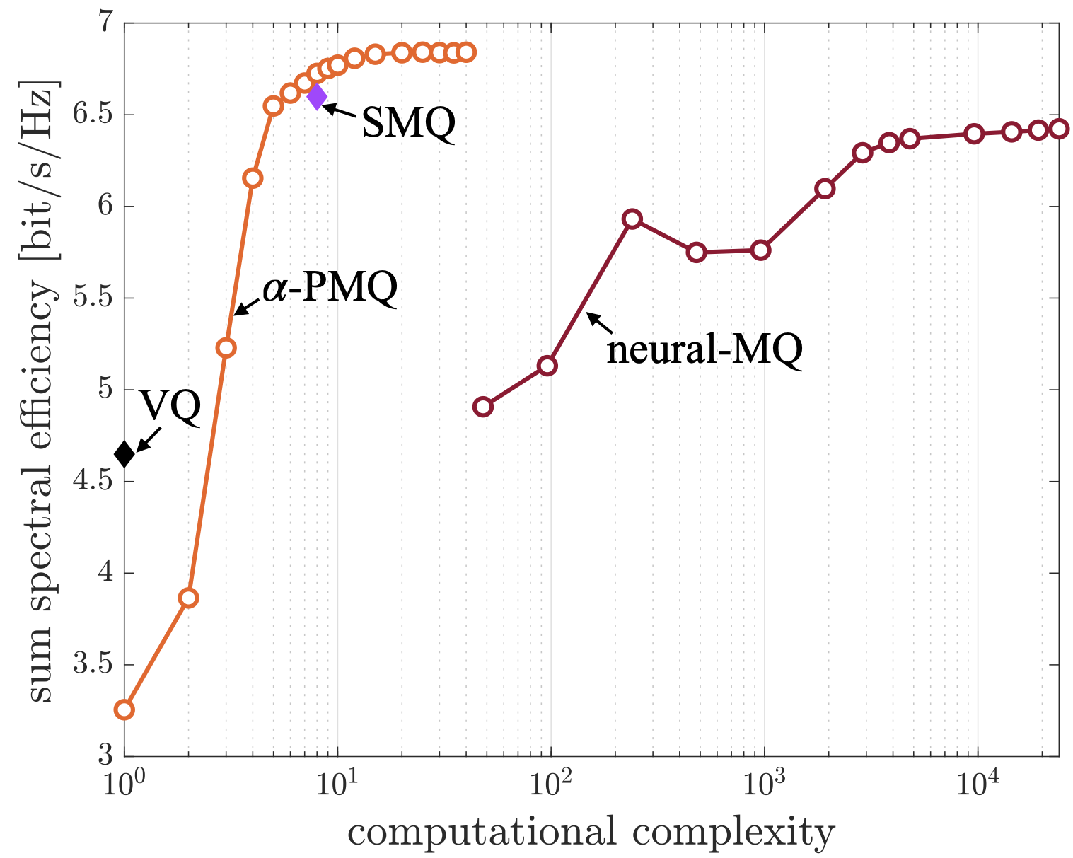
First, we study the spectral efficiency attained by different PC-based fronthaul quantization schemes against the computational complexity of fronthaul quantization. To this end, we consider the number of operations on a parallel processor, whereby parallel operation at different subprocessors are counted only once. We recall that Table I reviews the complexity measures for all schemes.
In Fig. 5, we assume multi-antenna UEs equipped with antennas with data stream per each UE, served by RUs equipped with antennas with fronthaul capacity . We set for -PMQ, and we vary the complexity of -PMQ and neural-MQ by increasing the number of iterations (Algorithm 1) and the number of GD steps (Algorithm 2), respectively. Accordingly, all the other schemes provide a single point in the performance-complexity trade-off. MQ is not shown in the figures due to excessive computational complexity.
It can be seen from the figure that, in this low-fronthaul capacity regime, for all spectral efficiency larger than around bit/s/Hz, -PMQ outperforms the other schemes, only VQ can achieve a higher computational efficiency but only in the very low spectral efficiency regime.
VI-B Higher-Fronthaul Capacity Regime: Comparison Between CP and PC
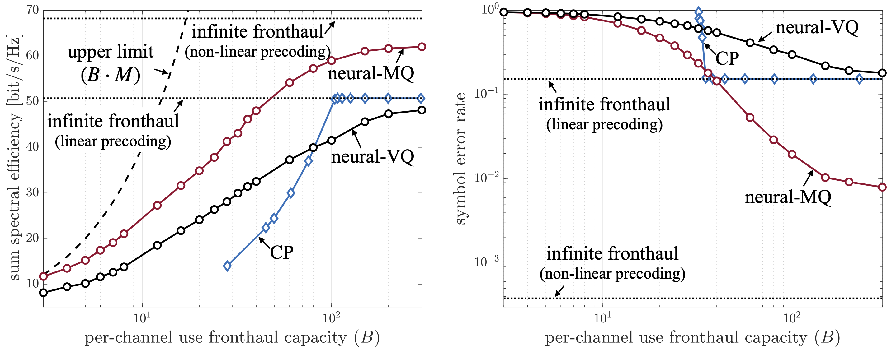
In this subsection, focusing on the high-fronthaul capacity regime, we compare neural-MQ to (i) infinite-fronthaul benchmarks; (ii) CP; and (iii) neural-VQ (see Appendix A).
For CP, we consider four different standard levels of precoding sharing, namely , while fixing the quantization level to [4]. In order to further examine the behavior of CP, we also considered the non-standard choices bits for , and for . We design the precoding matrix for CP by first evaluating the averaged channel matrix across channel uses, and then applying the MMSE precoding scheme [33, 34].
In Fig. 6, we show both sum spectral efficiency (left) and symbol error rate (right). For the fronthaul overhead (11) of CP, we assume channel coding with rate . This choice is dictated by the fact that a modulation scheme with symbols is approximately sufficient to achieve capacity [35].
Neural-MQ is seen to outperform CP in all fronthaul capacity regimes, while CP outperforms neural-VQ in the regime of , which highlights the importance of MQ. Note that both neural-VQ and CP cannot outperform the linear precoding benchmark, unlike the proposed neural-MQ.
Furthermore, neural-MQ approaches the performance of the infinite-fronthaul capacity with non-linear precoding benchmark as the fronthaul capacity increases, while neural-VQ approaches the infinite-fronthaul capacity benchmark under linear precoding. This validates the effectiveness of the proposed sum-EI criterion (42) in ensuring interference management, as well as of the proposed neural-codebook design, which can leverage the benefits of non-linear precoding.
VI-C Impact of Number of Gradient Descent Steps for Neural-MQ
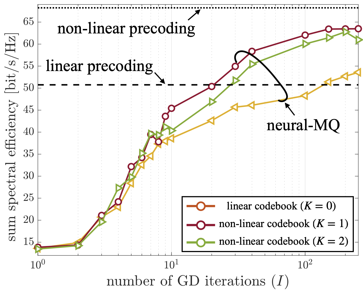
To provide further insights into the design of neural-MQ, we now study the impact of number of gradient descent steps in (47) on the performance of neural-MQ. We further compare the performance over different architectures of the neural codebook by varying the number of hidden layers . Note that corresponds to a linear mapping (look-up table) from bits to codewords.
Fig. 7 shows that, under a sufficiently large fronthaul capacity, here , and number of GD iterations (), neural-MQ outperforms linear precoding with infinite-fronthaul capacity, even with a linear mapping (look-up table) . Furthermore, a single hidden layer is observed to perform the best, outperforming the linear precoding with infinite-fronthaul capacity with less number of GD iterations ().
VI-D Generalization Capacity of Neural-MQ
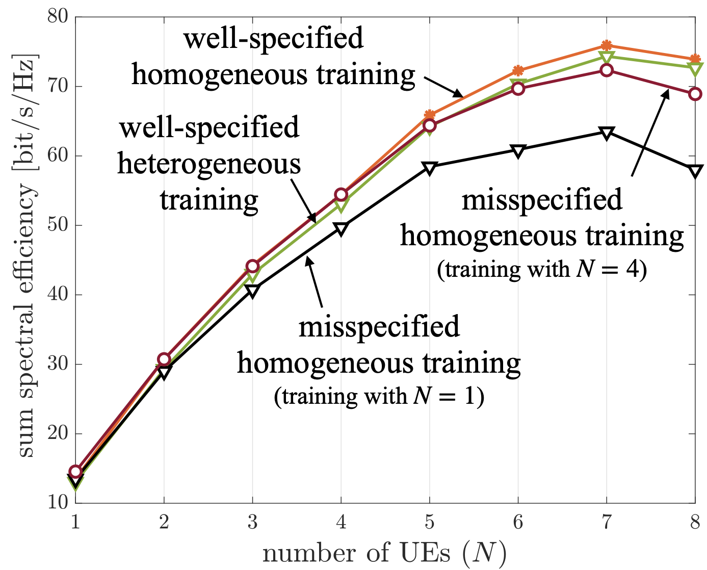
We now investigate the generalization capacity of neural-MQ by changing the number of UEs between training and testing. Specifically, in Fig. 8, we consider the following scenarios: (i) well-specified homogeneous training condition, in which we have no discrepancy between the fixed number of UEs during training and testing; (ii) misspecified homogeneous training conditions, in which training assumes a number of UEs equal to either or , while testing for UEs; (iii) well-specified heterogeneous training conditions, in which we train and test neural-MQ by using data set that consists of the same number of UEs.
Well-specified homogeneous training is seen to yield the best performance, with similar performance achieved also with well-specified heterogeneous training. While misspecified homogeneous training that assumes a single UE performs poorly when the number of UEs increases (), assuming UEs during training is sufficient to obtain good performance when testing with either smaller or larger numbers of UEs. The observed generalization capacity of neural-MQ can be understood by noting that the main role of neural-MQ is interference management, which depends less strongly on exact number of UEs and more on aspects such as the placement of RUs.
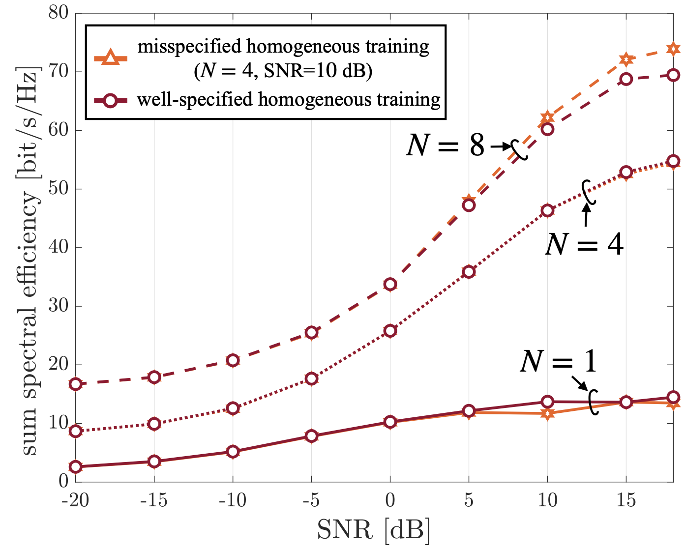
Next, we study the generalization capacity of neural-MQ by changing the total SNR from dB to dB. In a manner similar to Fig. 8, we consider (i) well-specified homogeneous training, i.e., no discrepancy between training and testing for both number of UEs as well as SNR, and (ii) misspecified homogeneous training in which training is done only by assuming and dB. It can be concluded from Fig. 9 that the considered misspecified homogeneous training is sufficient to obtain performance comparable to the well-specified homogeneous case. Robustness to different SNRs is again attributed to the main task of neural-MQ being interference management.
VII Conclusion
In this paper, we have proposed scalable MQ solutions for PC strategies in cell-free massive MIMO. The first approach, -PMQ, which has computational complexity growing exponentially in the per-RU fronthaul rate, outperforms all the other benchmarks including VQ [7] (e.g., sum spectral efficiency, with marginally increased complexity) and SMQ [7] (e.g., sum spectral efficiency, with slightly increased complexity), under conditions in which the original MQ [7] becomes infeasible due to large number of RUs (e.g., ).
The second proposed approach, neural-MQ, has computational complexity that grows linearly in the fronthaul sum-rate, and hence it can be applied in higher per-RU fronthaul regimes for which -PMQ is not feasible. Neural-MQ was seen to always outperform CP, irrespective of the fronthaul capacity (up to sum spectral efficiency under the same fronthaul capacity).
Appendix A Neural Vector Quantization
Neural-VQ follows the same procedure as in neural-MQ while the only difference coming from the objective of the minimization in (36), i.e.,
| (48) |
from which we have the quantized vector for RU as
| (49) |
In a manner similar to neural-MQ, we relax the problem by considering the optimization
| (50) |
which can again be solved via GD with temperature annealing as shown in Algorithm 3. It can be easily checked that the computational complexity of neural-VQ, , is less than VQ, , under high fronthaul capacity regime.
| (51) |
References
- [1] O. Simeone, N. Levy, A. Sanderovich, O. Somekh, B. M. Zaidel, H. V. Poor, and S. Shamai, “Cooperative wireless cellular systems: An information-theoretic view,” Foundations and Trends® in Communications and Information Theory, vol. 8, no. 1-2, pp. 1–177, 2012.
- [2] H. Q. Ngo, G. Interdonato, E. G. Larsson, G. Caire, and J. G. Andrews, “Ultra-dense cell-free massive MIMO for 6G: Technical overview and open questions,” arXiv preprint arXiv:2401.03898, 2024.
- [3] V. Q. Rodriguez, F. Guillemin, A. Ferrieux, and L. Thomas, “Cloud-ran functional split for an efficient fronthaul network,” in Proc. IEEE International Wireless Communications and Mobile Computing (IWCMC), Limassol, Cyprus, June 2020.
- [4] A. Grönland, B. Klaiqi, and X. Gelabert, “Learning-based latency-constrained fronthaul compression optimization in C-RAN,” in Proc. IEEE 28th International Workshop on Computer Aided Modeling and Design of Communication Links and Networks (CAMAD), Edinburgh, Scotland, Nov. 2023.
- [5] M. Koziol, “5G “open” standards are in play—just how open are they?” in IEEE Spectrum, 2023.
- [6] S.-H. Park, O. Simeone, O. Sahin, and S. Shamai, “Joint precoding and multivariate backhaul compression for the downlink of cloud radio access networks,” IEEE Transactions on Signal Processing, vol. 61, no. 22, pp. 5646–5658, 2013.
- [7] W. Lee, O. Simeone, J. Kang, and S. Shamai, “Multivariate fronthaul quantization for downlink C-RAN,” IEEE Transactions on Signal Processing, vol. 64, no. 19, pp. 5025–5037, 2016.
- [8] R. Qiao, T. Jiang, and W. Yu, “Meta-learning-based fronthaul compression for cloud radio access networks,” IEEE Transactions on Wireless Communications (Early Access), 2024.
- [9] A. Sanderovich, O. Somekh, H. V. Poor, and S. Shamai, “Uplink macro diversity of limited backhaul cellular network,” IEEE Transactions on Information Theory, vol. 55, no. 8, pp. 3457–3478, 2009.
- [10] Y. Khorsandmanesh, E. Björnson, and J. Jaldén, “Quantization-aware precoding for MU-MIMO with limited-capacity fronthaul,” in Proc. IEEE International Conference on Acoustics, Speech and Signal Processing (ICASSP), Singapore, Singapore, May 2022.
- [11] Ö. T. Demir, M. Masoudi, E. Björnson, and C. Cavdar, “Cell-free massive MIMO in O-RAN: Energy-aware joint orchestration of cloud, fronthaul, and radio resources,” IEEE Journal on Selected Areas in Communications, vol. 42, no. 2, pp. 356 – 372, 2024.
- [12] M. Bashar, A. Akbari, K. Cumanan, H. Q. Ngo, A. G. Burr, P. Xiao, M. Debbah, and J. Kittler, “Exploiting deep learning in limited-fronthaul cell-free massive MIMO uplink,” IEEE Journal on Selected Areas in Communications, vol. 38, no. 8, pp. 1678–1697, 2020.
- [13] N. Arad and Y. Noam, “Precode and quantize channel state information sharing for cloud radio access networks,” in Proc. IEEE International Conference on Communications (ICC), Kansas City, MO, USA, May 2018.
- [14] F. Wiffen, W. H. Chin, and A. Doufexi, “Distributed dimension reduction for distributed massive MIMO C-RAN with finite fronthaul capacity,” in Proc. IEEE 2021 55th Asilomar Conference on Signals, Systems, and Computers, Virtual Conference, Nov. 2021.
- [15] J. Liu, S. Zhou, J. Gong, Z. Niu, and S. Xu, “Graph-based framework for flexible baseband function splitting and placement in C-RAN,” in Proc. IEEE International Conference on Communications (ICC). IEEE, 2015, pp. 1958–1963.
- [16] J. Kang, O. Simeone, J. Kang, and S. Shamai, “Fronthaul compression and precoding design for C-RANs over ergodic fading channels,” IEEE Transactions on Vehicular Technology, vol. 65, no. 7, pp. 5022–5032, 2015.
- [17] F. W. Murti, S. Ali, G. Iosifidis, and M. Latva-Aho, “Learning-based orchestration for dynamic functional split and resource allocation in vRANs,” in Proc. Joint European Conference on Networks and Communications & 6G Summit (EuCNC/6G Summit), Grenoble, France, June 2022.
- [18] E. Björnson and L. Sanguinetti, “Scalable cell-free massive MIMO systems,” IEEE Transactions on Communications, vol. 68, no. 7, pp. 4247–4261, 2020.
- [19] P. Parida and H. S. Dhillon, “Cell-free massive MIMO with finite fronthaul capacity: A stochastic geometry perspective,” IEEE Transactions on Wireless Communications, vol. 22, no. 3, pp. 1555–1572, 2022.
- [20] J. Lorca and L. Cucala, “Lossless compression technique for the fronthaul of LTE/LTE-advanced cloud-ran architectures,” in Proc. IEEE 14th International Symposium on a World of Wireless, Mobile and Multimedia Networks (WoWMoM), Madrid, Spain, June 2013.
- [21] O. Simeone, Machine Learning for Engineers. Cambridge University Press, 2022.
- [22] F. T. Leighton, “A graph coloring algorithm for large scheduling problems,” Journal of Research of the National Bureau of Standards, vol. 84, no. 6, p. 489, 1979.
- [23] F. Alet, T. Lozano-Pérez, and L. P. Kaelbling, “Modular meta-learning,” in Proc. Conference on Robot Learning (CoRL), Zürich, Switzerland, Oct. 2018.
- [24] I. Nikoloska and O. Simeone, “Modular meta-learning for power control via random edge graph neural networks,” IEEE Transactions on Wireless Communications, vol. 22, no. 1, pp. 457–470, 2022.
- [25] A. Griewank, “Some bounds on the complexity of gradients, jacobians, and hessians,” in Complexity in Numerical Optimization. World Scientific, 1993, pp. 128–162.
- [26] S. S. Christensen, R. Agarwal, E. De Carvalho, and J. M. Cioffi, “Weighted sum-rate maximization using weighted MMSE for MIMO-BC beamforming design,” IEEE Transactions on Wireless Communications, vol. 7, no. 12, pp. 4792–4799, 2008.
- [27] C. Feng, W. Shen, J. An, and L. Hanzo, “Weighted sum rate maximization of the mmWave cell-free MIMO downlink relying on hybrid precoding,” IEEE Transactions on Wireless Communications, vol. 21, no. 4, pp. 2547–2560, 2021.
- [28] A. Gholami, S. Kim, Z. Dong, Z. Yao, M. W. Mahoney, and K. Keutzer, “A survey of quantization methods for efficient neural network inference,” in Low-Power Computer Vision. Chapman and Hall/CRC, 2022, pp. 291–326.
- [29] D. A. Schmidt, M. Joham, and W. Utschick, “Minimum mean square error vector precoding,” European Transactions on Telecommunications, vol. 19, no. 3, pp. 219–231, 2008.
- [30] M. Grant and S. Boyd, “Graph implementations for nonsmooth convex programs,” in Recent Advances in Learning and Control, ser. Lecture Notes in Control and Information Sciences, V. Blondel, S. Boyd, and H. Kimura, Eds. Springer-Verlag Limited, 2008, pp. 95–110, http://stanford.edu/~boyd/graph_dcp.html.
- [31] D. P. Kingma and J. Ba, “Adam: A method for stochastic optimization,” in Proc. 3rd International Conference on Learning Representations (ICLR), Banff, AB, Canada, May 2014.
- [32] 3GPP, “Study on channel model for frequencies from 0.5 to 100 GHz,” TR 38.901, Release 16.1.
- [33] M. Vu and A. Paulraj, “MIMO wireless linear precoding,” IEEE Signal Processing Magazine, vol. 24, no. 5, pp. 86–105, 2007.
- [34] K. Venugopal, N. González-Prelcic, and R. W. Heath, “Optimal frequency-flat precoding for frequency-selective millimeter wave channels,” IEEE Transactions on Wireless Communications, vol. 18, no. 11, pp. 5098–5112, 2019.
- [35] S. Y. Le Goff, “Signal constellations for bit-interleaved coded modulation,” IEEE Transactions on Information Theory, vol. 49, no. 1, pp. 307–313, 2003.
- [36] J. Duchi, E. Hazan, and Y. Singer, “Adaptive subgradient methods for online learning and stochastic optimization.” Journal of Machine Learning Research, vol. 12, no. 7, 2011.
- [37] N. Shlezinger, Y. C. Eldar, and S. P. Boyd, “Model-based deep learning: On the intersection of deep learning and optimization,” IEEE Access, vol. 10, pp. 115 384–115 398, 2022.
- [38] D. Jain, K. M. Choromanski, K. A. Dubey, S. Singh, V. Sindhwani, T. Zhang, and J. Tan, “Mnemosyne: Learning to train transformers with transformers,” in Proc. Advances in Neural Information Processing Systems (NeurIPS), Vancouver, British Columbia, Canada, Dec. 2024.