Intravalley spin-polarized superconductivity in rhombohedral tetralayer graphene

Abstract

We study the intravalley spin-polarized superconductivity in rhombohedral tetralayer graphene, which has been discovered experimentally in Han $et$ $al$ arXiv:2408.15233. We construct a minimal model for the intravalley spin-polarized superconductivity, assuming a simplified anisotropic interaction that depends only on the angle between the incoming and outgoing momenta. Despite the absence of Fermi surface nesting, we show that the superconductivity appears near the Van Hove singularity with the maximal $T_{c}$ near a bifurcation point of the peaks in the density of states. We identify the topological $p+ip$, topological $h+ih$, and the non-topological nodal $f$-wave pairings as the possible states, which are all pair density wave orders due to the intravalley nature. Furthermore, these pair density wave orders require a finite attractive threshold for superconductivity, resulting in narrow superconducting regions, consistent with experimental findings. We discuss the possible pairing mechanisms and point out that the Kohn-Luttinger mechanism is a plausible explanation for the intravalley spin-polarized superconductivity in the rhombohedral tetralayer graphene.

Introduction.— Superconductivity (SC) is one of the most important and intriguing quantum phenomena in condensed matter and material physics. Since the initial discovery of SC in the magic-angle twisted bilayer graphene [1], observable two-dimensional (2D) SC ($T_{c}>20$ mK) has been reported in various twisted and untwisted van der Waals multilayer systems [2, 3] (e.g., twisted multilayer graphene [4, 5, 6, 7, 8, 9, 10, 11, 12, 13, 14], twisted bilayer WSe₂ [15, 16], Bernal bilayer graphene [17, 18, 19, 20, 21], and rhombohedral trilayer [22, 23, 24] and tetralayer graphene [25]). Notably, the untwisted graphene multilayers are promising systems for studying unconventional SC because of the ability to control the electronic band structures through the displacement field and the lower disorder nature.

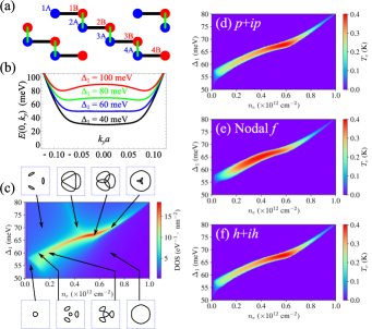
Figure 1: Stacking pattern, dispersion, density of states, and SC in the electron-doped rhombohedral tetralayer graphene. (a) The rhombohedral stacking pattern of tetralayer graphene. The blue (red) dots sublattice A (B) sites; the layer is labeled by 1, 2, 3, and 4 from top to bottom. (b) The dispersion of the first electron band (from charge neutrality) along $y$ direction relative to the valley $+K$ point with several $\Delta_{1}$, tuned by the applied displacement field. $a$ is the graphene lattice constant. (c) Density of states (assuming spin and valley polarization) as a function of doping density ($n_{e}$) and $\Delta_{1}$. Several representative Fermi surfaces are also illustrated, showing the complicated nature of single-particle Lifshitz transitions at the VHSs. (d) $T_{c}$ of $p+ip$ SC as a function of $n_{e}$ and $\Delta_{1}$ with $g_{1}=160$ meV.nm². (e) $T_{c}$ of nodal $f$ SC as a function of $n_{e}$ and $\Delta_{1}$ with $g_{1}=135$ meV.nm². (d) $T_{c}$ of $h+ih$ SC as a function of $n_{e}$ and $\Delta_{1}$ with $g_{1}=160$ meV.nm². The results in (d)-(f) suggest that intravalley spin-polarized SC is strongest near the VHS at $\Delta_{1}=67$ meV that shows six Fermi contour crossing points in the $\bm{\mathrm{k}}$ space. (d) and (f) show the identical $T_{c}$’s within our numerical accuracy. We have used $\approx 2\times 10^{6}$ $k$ points and assumed spin and valley polarization in (c)-(f).

Superconductivity in the graphene-based materials (and moiré transition metal dichalcogenides) often requires intervalley pairings between two time-reversal related bands [26, 27, 28, 29, 30, 31, 32, 33, 34, 35, 36, 37, 38, 39, 40, 41, 42, 43, 44, 45, 46, 47, 48, 49, 50] because the Fermi surface nesting guarantees zero-temperature SC in the presence of an arbitrarily small attractive interaction. A recent rhombohedral tetralayer graphene experiment discovers a novel time-reversal broken SC (with $T_{c}\sim 300$ mK), emerging from a spin-polarized valley-polarized normal state [51]. Such a superconducting order persists a large out-of-plane magnetic field ($B_{\perp,c}>0.9$ T) and shows hysteresis of $R_{xy}$ under an out-of-plane magnetic field. The experimental evidence suggests a possible chiral topological SC [52, 53, 54, 55], which has not been conclusively confirmed in any existing experiment. At the conceptual level, the existence of SC from intravalley pairing is also highly nontrivial. The trigonal warping in graphene multilayers generically results in non-circular Fermi surfaces [56], sabotaging the Fermi surface nesting for pairings.

In this Letter, we study the possible SC arising from a spin-polarized valley-polarized normal state in the rhombohedral stacked tetralayer graphene [Fig. 1(a)], motivated by the chiral SC experiment [51]. First, we analyze the single-particle band structure in the electron doping [Fig. 1(b)] and reveal a multitude of Fermi surface transitions associated with Van Hove singularities (VHSs) as shown in Fig. 1(c). Then, we construct a minimal toy model that describes the intravalley spin-polarized pairing with an odd angular momentum, e.g., $p$-wave, $f$-wave, and $h$-wave. Based on a mean-field analysis, we identify the “magic condition” that favors intravalley SC without Fermi surface nesting. If the $p$-wave pairing channel dominates, the resulting SC is the $p+ip$ topological SC [52, 53, 54, 55] (the class D in the ten-fold way classification [57, 58, 54]), manifesting chiral Majorana edge states. If the $f$-wave channel dominates, the SC is a nodal topologically trivial SC. For the $h$-wave case, we find a $h+ih$ chiral topological SC of class D, similar to the $p$-wave case. We also investigate the non-BCS nature of the intravalley SC and show that a finite threshold is required for realizing SC, generically resulting in narrow SC regions. Finally, we discuss possible microscopic mechanisms for the intravalley SC observed in the experiment.

Single-particle model.— We study the rhombohedral tetralayer graphene (i.e., with a chiral ABCA stacking pattern [56]). The single-particle Hamiltonian of valley $\tau K$ and spin $s$ can be described by

$$\hat{H}^{(\tau,s)}_{0}=\sum_{\bm{\mathrm{k}}}\Psi^{\dagger}(\bm{\mathrm{k}})\hat{h}^{(\tau)}(\bm{\mathrm{k}})\Psi(\bm{\mathrm{k}}),$$ (1)

where $\bm{\mathrm{k}}=(k_{x},k_{y})$ is the 2D wavevector relative to the valley wavevector $\tau\bm{\mathrm{K}}$, $\Psi$ is a 8-dimensional field incorporating layers and sublattices, and $\hat{h}^{(\tau)}(\bm{\mathrm{k}})$ is a 8-by-8 matrix characterizing the details of band structures [59, 60, 61] (see Supplemental Material [62]). The low energy sites are the 1A (A sublattice on the top layer) and the 4B (B sublattice on the bottom layer) sites [labeled in Fig. 1(a)] because the interlayer hybridization [green bonds in Fig. 1(a)] generically pushes other sites to higher energies. The electronic bands can be tuned by a perpendicular electric field (i.e., a displacement field), which induces imbalanced electrostatic potential in layers, described by a single parameter $\Delta_{1}$. With a sufficiently large $|\Delta_{1}|$ (which is always true in this Letter), the layer and sublattice are also polarized in the low-energy bands. In our convention, the energy difference between the top and bottom layers is $2|\Delta_{1}|$, and the low-energy electron band corresponds to the 4B sites for $\Delta_{1}>0$.

The electron-doped band structure is sensitive to the value of $\Delta_{1}$. As shown in Fig. 1(b), the electron band bottom can become extremely flat for $\Delta_{1}\approx 60$ meV. With a more careful analysis, we find that the flattest band, defined by the largest density of states (DOS), is around $\Delta_{1}=67$ meV, corresponding to a bifurcation point of the VHS peaks in Fig. 1(c). The corresponding Fermi surface at that point shows six crossings. (See Ref. [60] for similar single-particle results.) Notably, the Fermi surfaces in the same regime are not circular but typically manifest complicated Fermi surfaces [Fig. 1(c)] that reveal the absence of Fermi surface nesting for an intravalley pairing SC. However, SC can still be realized without exact Fermi surface nesting as discussed in the pair density wave (PDW) orders [63] and the recently proposed interband SC in spin-orbit magic-angle twisted bilayer graphene [64]. Next, we develop a minimal pairing model and examine the possible intravalley spin-polarized SC without Fermi surface nesting.

Pairing interaction.— We are interested in pairing within the same valley and the same spin. In the presence of a large $|\Delta_{1}|$, the layer and sublattice are also polarized, leaving no internal degrees of freedom in this problem. In our convention, the low-energy electron-doped band is polarized to the 4B site. We consider the $+K$ valley and up spin without loss of generality. The intravalley spin-polarized pairing Hamiltonian (interaction in the Cooper channel) can be expressed by

$$\hat{H}_{I}=\frac{1}{2\mathcal{A}}\sum_{\bm{\mathrm{k}},\bm{\mathrm{k}}^{\prime}}V_{\bm{\mathrm{k}},\bm{\mathrm{k}}^{\prime}}\psi^{\dagger}(\bm{\mathrm{k}})\psi^{\dagger}(-\bm{\mathrm{k}})\psi(-\bm{\mathrm{k}}^{\prime})\psi(\bm{\mathrm{k}}^{\prime}),$$ (2)

where $\mathcal{A}$ is the 2D area, $V_{\bm{\mathrm{k}},\bm{\mathrm{k}}^{\prime}}$ is the pairing interaction and $\psi$ is the fermionic field of 4B site with $+K$ valley and up spin. We have suppressed the layer, sublattice, and spin indexes of $\psi$.

Computation with the general $V_{\bm{\mathrm{k}},\bm{\mathrm{k}}^{\prime}}$ is challenging, especially since a very fine $\bm{\mathrm{k}}$ mesh is required for describing the details of VHS. Thus, we consider a simplified pairing interaction that depends only on the relative angle between $\bm{\mathrm{k}}$ and $\bm{\mathrm{k}}^{\prime}$ and decompose the pairing interaction in terms of Fourier harmonics as follows:

$$V_{\bm{\mathrm{k}},\bm{\mathrm{k}}^{\prime}}\rightarrow -\sum_{l=0}^{\infty}g_{l}\cos\left[l\left(\phi_{\bm{\mathrm{k}}}-\phi_{\bm{\mathrm{k}}^{\prime}}\right)\right],$$ (3)

where $g_{l}$ is the attractive pairing interaction with angular momentum $l$, and $\phi_{\bm{\mathrm{k}}}$ is the angle of $\bm{\mathrm{k}}$ relative to the $x$ axis. Equation (3) is the main assumption in this Letter, which ignores the $|\bm{\mathrm{k}}|$ and $|\bm{\mathrm{k}}^{\prime}|$ dependence in the pairing interaction [65]. As we will discuss later, the simplified interaction allows a very efficient formulation for the numerical computation of the transition temperature $T_{c}$.

For spin-polarized SC, only $g_{l}$’s with odd $l$’s are relevant because of the antisymmetrization. The situation here is different from the intervalley pairing in the graphene-based material, in which valley and sublattice may avoid antisymmetrization at the orbital level, resulting in essentially $\bm{\mathrm{k}}$ independent pairing [28, 66]. In our calculations, we treat the values of $g_{1}$, $g_{3}$, and $g_{5}$ as tunable parameters and focus on general features of the superconducting states.

The pairing interaction, Eq. (3), can be factorized, using the trigonometric identity $\cos[l(\phi_{\bm{\mathrm{k}}}-\phi_{\bm{\mathrm{k}}^{\prime}})]=\cos\left(l\phi_{\bm{\mathrm{k}}}\right)\cos\left(l\phi_{\bm{\mathrm{k}}^{\prime}}\right)+\sin\left(l\phi_{\bm{\mathrm{k}}}\right)\sin\left(l\phi_{\bm{\mathrm{k}}^{\prime}}\right)$. Then, we perform Hubbard-Stratonovich decoupling for each component and consider the static translational invariant saddle point solution, equivalent to the standard mean-field theory. The single-band projection onto the low-energy electron band is also performed. Finally, the fermions are integrated out, and a Landau theory is constructed by perturbing the ordering parameter. The detailed derivation is provided in Supplemental Material [62]. We summarize the main results in the following.

For a given pairing channel $l$, the Landau free energy density is expressed by

$$\frac{\mathcal{F}}{\mathcal{A}}\!=\!\left[\begin{array}[]{cc}\Delta_{l,1}^{*}&\Delta_{l,2}^{*}\end{array}\right]\!\left[\begin{array}[]{cc}\frac{1}{2g_{l}}-a_{1}(T)&-a_{12}(T)\\[5.69054pt] -a_{12}(T)&\frac{1}{2g_{l}}-a_{2}(T)\end{array}\right]\!\left[\begin{array}[]{c}\Delta_{l,1}\\[5.69054pt] \Delta_{l,2}\end{array}\right]\!+\!O(\Delta^{4}),$$ (9)

where the expressions of $a_{1}$, $a_{2}$, and $a_{12}$ are provided in [62], the order parameters are defined by

$$\Delta_{l,1}= -\frac{2g_{l}}{\mathcal{A}}\sum_{\bm{\mathrm{k}}}^{\prime}\cos\left(l\phi_{\bm{\mathrm{k}}}\right)\left\langle\psi(-\bm{\mathrm{k}})\psi(\bm{\mathrm{k}})\right\rangle,$$ (10a)

$$\Delta_{l,2}= -\frac{2g_{l}}{\mathcal{A}}\sum_{\bm{\mathrm{k}}}^{\prime}\sin\left(l\phi_{\bm{\mathrm{k}}}\right)\left\langle\psi(-\bm{\mathrm{k}})\psi(\bm{\mathrm{k}})\right\rangle.$$ (10b)

In Eq. (10), the summation $\sum_{\bm{\mathrm{k}}}^{\prime}$ is over half of the $\bm{\mathrm{k}}$ mesh with $\bm{\mathrm{k}}=0$ excluded. The linearized gap equation can be obtained by the vanishing quadratic term in Eq. (9), which is given by

$$\left[\begin{array}[]{c}\Delta_{l,1}\\[5.69054pt] \Delta_{l,2}\end{array}\right]=(2g_{l})\left[\begin{array}[]{cc}a_{1}(T_{c})&a_{12}(T_{c})\\[5.69054pt] a_{12}(T_{c})&a_{2}(T_{c})\end{array}\right]\left[\begin{array}[]{c}\Delta_{l,1}\\[5.69054pt] \Delta_{l,2}\end{array}\right].$$ (17)

Note that the appearance of factor of 2 in $g_{l}$ is due to summing over half of the $\bm{\mathrm{k}}$ mesh, avoiding double counting in the single-particle term. The eigenvector of Eq. (17) indicates the pairing symmetry. In the case of doubly degenerate solutions, we need to analyze the $O(\Delta^{4})$ part of Eq. (9), as we will discuss in the $p$-wave case later.

The tractable expression of Eq. (17) is a consequence of the simplified pairing interaction in Eq. (3) as discussed in [62]. For a general $V_{\bm{\mathrm{k}},\bm{\mathrm{k}}^{\prime}}$, one needs to diagonalize a dense matrix with the dimension proportional to the number of $\bm{\mathrm{k}}$ points [36, 67, 61] (around $2\times 10^{6}$ $\bm{\mathrm{k}}$ points are used in this Letter), which is a numerically challenging task. We also emphasize that a fine $\bm{\mathrm{k}}$-space mesh is required as the VHS is indispensable in our theory.

In our model, $g_{l}$’s are treated as free parameters. Specifically, we focus on the $p$-wave ($l=1$), $f$-wave ($l=3$), and $h$-wave ($l=5$) pairing channels. We aim to investigate the conditions of realizing an intravalley spin-triplet SC (e.g., $g_{l}$, $\Delta_{1}$, and $n_{e}$) based on our minimal model, providing some constraints on the candidate microscopic theories. The angular momentum mixing pairing (such as $p+f$) will not be discussed in this Letter.

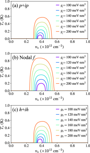
Figure 2: $T_{c}$ as a function of doping with $\Delta_{1}=65$ meV and a few representative values of $g_{l}$’s. (a) The $p$-wave case. (b) The $f$-wave case. In both cases, we vary the value of $g_{l}$ and plot the corresponding $T_{c}$ for each $n_{e}$.

Topological chiral SC: $p+ip$ and $h+ih$ pairings. — We first investigate the $p$-wave case ($l=1$). The two components of order parameters correspond to $p_{x}$ ($\Delta_{1,1}$) and $p_{y}$ ($\Delta_{1,2}$) orders. Generally, we find that $p_{x}$ and $p_{y}$ components are degenerate (within numerical accuracy), indicating that the importance of analyzing the quartic terms, $O(\Delta^{4})$, in Eq. (9). We find that the $O(\Delta^{4})$ terms can be expressed by $u(T)\left(|\Delta_{l,1}|^{2}+|\Delta_{l,2}|^{2}\right)^{2}+u^{\prime}(T)\left(\Delta_{l,1}\Delta_{l,2}^{*}-\Delta_{l,2}\Delta_{l,1}^{*}\right)^{2}$ with $u(T)>0$ and $u^{\prime}(T)>0$. The positivity of $u^{\prime}(T)$ favors a formation of a chiral $p$-wave order, realizing a 2D topological superconductor of class $D$ with chiral Majorana edge states on the sample boundary [52, 53, 54, 55]. This state is distinct from the conventional $p+ip$ SC because the Cooper pairs from intravalley pairing carry finite momenta, making it a PDW with the Fulde-Ferrel-like plane-wave order [63].

Now, we investigate the most favorable conditions for intravalley SC. In Fig. 1(d), we plot $T_{c}$ of the $p+ip$ SC as functions of the doping density $n_{e}$ and $\Delta_{1}$ for $g_{1}=160$ meV$\cdot$nm². We find that the peak of $T_{c}$ follows the VHS, and the maximal $T_{c}$ happens close to the largest density of states location at $\Delta_{1}\approx 67$ meV, the bifurcation point in the VHS peaks. Interestingly, the Fermi surface is not circular, indicating the absence of Fermi surface nesting. We also find that the situations manifesting nearly circular Fermi surfaces yield much weaker $T_{c}$. To understand the doping dependence further, we plot the $T_{c}$ as a function of the doping density $n_{e}$ at $\Delta_{1}=65$ meV In Fig. 2(a). We vary the value of $g_{1}$ and show how the value of $g_{1}$ influences $T_{c}$. Interestingly, the fading of $T_{c}$ at the boundary of superconducting dome is quite sharp, different from intervalley SC [26, 27, 28, 29, 30, 31, 35, 66, 37, 46]. We will discuss this property in depth later.

We also check the $h$-wave case ($l=5$) and show that a chiral $h+ih$ topological SC [52, 53, 54, 55] of class D is realized. Moreover, the linearized gap equation [Eq. (17)] yields the same $T_{c}$ (for the same $g_{l}$) as the $p$-wave case [as shown in Fig. 1(f) and Fig. 2(c)]. The identical results of the $p$-wave and $h$-wave reveal a hidden symmetry structure in our model. In fact, we find that the $T_{c}$ is identical for all odd $l$ that is not divisible by 3. This hidden symmetry is likely an artifact of our simplified interaction, which should be lifted by other perturbations.

Nodal SC: $f$-wave pairing.— We also investigate the possible $f$-wave SC in this model. The two components of the order parameters correspond to the weighting factors $\cos(3\phi_{\bm{\mathrm{k}}})$ ($\Delta_{3,1}$) and $\sin(3\phi_{\bm{\mathrm{k}}})$ ($\Delta_{3,2}$). We find that $\Delta_{3,2}$ generally dominates over the $\Delta_{3,1}$ regardless of $\Delta_{1}$ and $n_{e}$, realizing a nodal $f$-wave SC. The resulting superconducting state is topologically trivial but breaks both time-reversal and inversion symmetries because of the intravalley nature of the state. The intravalley nodal $f$-wave SC here can be viewed as a PDW with the Fulde-Ferrel-like plane-wave order, carrying a finite momentum.

In Fig. 1(e), we plot $T_{c}$ of the nodal $f$-wave SC as functions of the doping density $n_{e}$ and $\Delta_{1}$ for $g_{3}=135$ meV$\cdot$nm². Similar to the $p$-wave case, the peak of $T_{c}$ follows the VHS, and the maximal $T_{c}$ is near the bifurcation point of VHS peaks at $\Delta_{1}=67$ meV. We further plot the $T_{c}$ as a function of doping density $n_{e}$ at $\Delta_{1}=65$ meV in Fig. 2(b) with different values of $g_{3}$. Here, $T_{c}$ is higher for a given $g_{3}$ compared to the $T_{c}$ with the same value of $g_{1}$ in the $p$-wave case. Note that this does not suggest that $f$-wave is more favorable than $p$-wave. The values of $g_{1}$ and $g_{3}$ should be determined by a specific microscopic model. We also find the abrupt termination of SC in the $f$-wave case, signaling qualitatively different features from the intervalley pairing, which we discuss next.

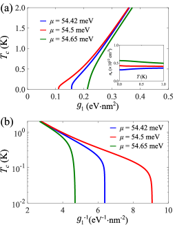
Figure 3: The non-BCS features of $p$-wave chiral SC. We consider $\Delta_{1}=65$ meV and a few representative values of the chemical potentials. (a) $T_{c}$ as a function of $g_{1}$. The results show a sharp termination of $T_{c}$, instead of the exponentially small $T_{c}$ in the BCS SC. Inset: The doping density ($n_{e}$) as a function of temperature. (b) $T_{c}$ as a function of $g_{1}^{-1}$. For each case, $T_{c}$ deviates from the well-known exponential dependence for a sufficiently large $g_{1}^{-1}$ (equivalently, a sufficiently small $g_{l}$). The results here clearly indicate the existence of a threshold coupling constant below which SC vanishes exactly at $T=0$. The threshold value is non-universal, depending on $\mu$, $\Delta_{1}$, and other single-particle model parameters. The results of $f$-wave SC ($l=3$) are similar.

Non-BCS properties.— The intravalley SC discussed in this Letter possesses some fundamental differences from the intervalley SC that arise from time-reversal-related active bands. First, the exact Fermi surface nesting is lacking in our situation [see Fig. 1(c) for several representative Fermi surface contours], suggesting that SC is absent in the weak coupling limit. In Fig. 3(a), we show that the linearized gap equation of the $p$-wave case at a fixed $\mu$ yields a threshold value of $g_{l}$ below which SC is completely suppressed. The doping density $n_{e}$ for a fixed $\mu$ varies only slightly as lowering $T$. Thus, we conclude that there is a finite threshold for a fixed $n_{e}$ situation, also. We find similar results in other cases with $l>1$. In Fig. 3(b), we plot $T_{c}$ as a function of $g_{1}^{-1}$ and find that the results deviate from the exponential decaying behavior at some values of $g_{1}^{-1}$. Note that the celebrated BCS formula is given by $T_{c}\propto\exp\left(-1/\lambda\right)$, where $\lambda$ is the dimensionless BCS coupling constant. Evidently, the intravalley SC here is qualitatively different. The existence of a threshold for realizing SC explains the narrowness and sharp termination in the SC region, consistent with the experimental findings.

Discussion.— We construct and analyze a minimal model for the intravalley spin-polarized SC, aiming to understand the unconventional SC in the electron-doped rhombohedral tetralayer graphene, specifically, the SC1 in Ref. [68]. Our results reveal that the intravalley SC is most favorable near the VHS, with the maximal $T_{c}$ found near the bifurcation point of VHS peaks ($\Delta_{1}\approx 67$ meV based on the single-particle band structure), corresponding to an optimal value of displacement strength, and possible pairing symmetries: $p+ip$ chiral topological SC, $h+ih$ chiral topological SC, and nodal $f$-wave SC. In addition, we find that the resulting SC requires a finite coupling strength, resulting in narrow superconducting regions consistent with the experimental findings.

In this Letter, we assume spin and valley polarized quarter metal as the normal state and adopt the single-particle band structure. Incorporating the band renormalization, the band structure acquires corrections, and the precise location and shape of SC region can be modified. Another important issue is that the microscopic interaction might not be the same as Eq. (3), and some $|\bm{\mathrm{k}}|$ dependence is anticipated. As long as the variation of $|\bm{\mathrm{k}}|$ is not significant, our model interaction can be viewed as an averaged version of the microscopic interaction, and the qualitative results should remain. For example, we expect that the intravalley SC is associated with VHS, and the VHS-assisted pairing [69, 70, 71, 72, 73] might be the key for intravalley SC, regardless of the details in the band renormalization or the precise form of pairing interaction.

We conclude this Letter by discussing the possible pairing mechanisms in the experiment [51]. First, the conventional phonon-mediated pairings [27, 28, 30, 36] are irrelevant as an anisotropic pairing interaction is required for an intravalley spin-polarized SC without any other internal degrees of freedom. In the experiment, the maximal $T_{c}$ is found in the device without any WSe₂, and the device with WSe₂ proximate to the electron band yields the weakest SC. The correlation between WSe₂ and $T_{c}$ suggest a possible repulsion-induced mechanism because WSe₂ provides a stronger dielectric screening, and SC is the strongest without WSe₂. The isospin fluctuation mechanism [74, 66, 75, 76, 77], which is commonly discussed in the graphene SC, is unlikely because spin and valley are both polarized in the normal state (at least for SC1 in Ref. [51]). Finally, we investigate the screened Coulomb interaction with RPA in the spirit of the Kohn-Luttinger mechanism [37, 50]. Using a small $\bm{\mathrm{k}}$ mesh and averaging over $\bm{\mathrm{k}}$, $\bm{\mathrm{k}}^{\prime}$ on a circle, we obtain a dominant $p$-wave pairing interaction with $g_{1}$ of order of 100 meV.nm². Using the model discussed in this Letter, a chrial topological $p+ip$ SC is realized with a maximal $T_{c}$ of order of 0.1 K, consistent with the experiment [51]. Thus, we speculate that the Kohn-Luttinger-like mechanism is responsible for the intravalley spin-polarized SC in the rhombohedral tetralayer graphene. The main thrust and findings of our work are independent of the microscopic mechanism for the triplet superconductivity, and a future systematic analysis incorporating the $|\bm{\mathrm{k}}|$-dependent pairing interaction deserves a separate detailed investigation in order to decisively establish whether a Kohn-Luttinger mechanism arising from the screened Coulomb interaction (as speculated here) is indeed operational here. Our work provides a simple systematic way for understanding the intravalley spin-polarized SC, which should motivate future experimental and theoretical studies.

Intravalley spin-polarized superconductivity in rhombohedral tetralayer graphene
SUPPLEMENTAL MATERIAL

I Single-particle model

The single-particle model $\hat{h}^{(\tau)}$ is expressed by

$$\hat{h}^{(\tau)}=\left[\begin{array}[]{cccccccc}\delta-\Delta_{1}&v_{0}\Pi_{\bm{\mathrm{k}}}^{\dagger}&v_{4}\Pi_{\bm{\mathrm{k}}}^{\dagger}&v_{3}\Pi_{\bm{\mathrm{k}}}&0&\frac{1}{2}\gamma_{2}&0&0\\ v_{0}\Pi_{\bm{\mathrm{k}}}&-\Delta_{1}&\gamma_{1}&v_{4}\Pi_{\bm{\mathrm{k}}}^{\dagger}&0&0&0&0\\ v_{4}\Pi_{\bm{\mathrm{k}}}&\gamma_{1}&-\frac{\Delta_{1}}{3}&v_{0}\Pi_{\bm{\mathrm{k}}}^{\dagger}&v_{4}\Pi_{\bm{\mathrm{k}}}^{\dagger}&v_{3}\Pi_{\bm{\mathrm{k}}}&0&\frac{1}{2}\gamma_{2}\\ v_{3}\Pi_{\bm{\mathrm{k}}}^{\dagger}&v_{4}\Pi_{\bm{\mathrm{k}}}&v_{0}\Pi_{\bm{\mathrm{k}}}&-\frac{\Delta_{1}}{3}&\gamma_{1}&v_{4}\Pi_{\bm{\mathrm{k}}}^{\dagger}&0&0\\ 0&0&v_{4}\Pi_{\bm{\mathrm{k}}}&\gamma_{1}&\frac{\Delta_{1}}{3}&v_{0}\Pi_{\bm{\mathrm{k}}}^{\dagger}&v_{4}\Pi_{\bm{\mathrm{k}}}^{\dagger}&v_{3}\Pi_{\bm{\mathrm{k}}}\\ \frac{1}{2}\gamma_{2}&0&v_{3}\Pi_{\bm{\mathrm{k}}}^{\dagger}&v_{4}\Pi_{\bm{\mathrm{k}}}&v_{0}\Pi_{\bm{\mathrm{k}}}&\frac{\Delta_{1}}{3}&\gamma_{1}&v_{4}\Pi_{\bm{\mathrm{k}}}^{\dagger}\\ 0&0&0&0&v_{4}\Pi_{\bm{\mathrm{k}}}&\gamma_{1}&\Delta_{1}&v_{0}\Pi_{\bm{\mathrm{k}}}^{\dagger}\\ 0&0&\frac{1}{2}\gamma_{2}&0&v_{3}\Pi_{\bm{\mathrm{k}}}^{\dagger}&v_{4}\Pi_{\bm{\mathrm{k}}}&v_{0}\Pi_{\bm{\mathrm{k}}}&\delta+\Delta_{1}\\ \end{array}\right],$$ (S9)

where $\Pi_{\bm{\mathrm{k}}}=\tau k_{x}+ik_{y}$ ($\tau=1,-1$ for valleys K and $-$K respectively), $v_{j}=\frac{\sqrt{3}}{2}\gamma_{j}a_{0}$, $\gamma_{j}$ is the bare hopping matrix element, and $a_{0}=0.246$ nm is the lattice constant of graphene. $\gamma_{0}=3.1$ eV, $\gamma_{1}=0.38$ eV, $\gamma_{2}=-0.015$ eV, $\gamma_{3}=-0.29$ eV, $\gamma_{4}=-0.141$ eV, and $\delta=-0.0105$ eV. The value of $\Delta_{1}$ corresponds to the out-of-plane displacement field. The basis of the matrix is (1A,1B,2A,2B,3A,3B,4A,4B) with the number representing the layer and A/B representing the sublattice. The band parameters here are obtained from Ref. [59] for the rhombohedral trilayer graphene. The model here is equivalent to Ref. [60] and Ref. [61] with $\Delta_{2}$ and $\Delta_{3}$ set to zero.

II Mean-field theory

The pairing interaction for the channel $l$ is given by

$$\hat{H}_{I,l}= \frac{-g_{l}}{2\mathcal{A}}\sum_{\bm{\mathrm{k}},\bm{\mathrm{k}}^{\prime}}\cos\left[l\left(\phi_{\bm{\mathrm{k}}}-\phi_{\bm{\mathrm{k}}^{\prime}}\right)\right]\psi^{\dagger}(\bm{\mathrm{k}})\psi^{\dagger}(-\bm{\mathrm{k}})\psi(-\bm{\mathrm{k}}^{\prime})\psi(\bm{\mathrm{k}}^{\prime})$$ (S10)

$$= \frac{-2g_{l}}{\mathcal{A}}\sum_{\bm{\mathrm{k}},\bm{\mathrm{k}}^{\prime}}^{\prime}\left\{\begin{array}[]{r}\left[\psi^{\dagger}(\bm{\mathrm{k}})\cos\left(l\phi_{\bm{\mathrm{k}}}\right)\psi^{\dagger}(-\bm{\mathrm{k}})\right]\left[\psi(-\bm{\mathrm{k}}^{\prime})\cos\left(l\phi_{\bm{\mathrm{k}}^{\prime}}\right)\psi(\bm{\mathrm{k}}^{\prime})\right]\\[5.69054pt] +\left[\psi^{\dagger}(\bm{\mathrm{k}})\sin\left(l\phi_{\bm{\mathrm{k}}}\right)\psi^{\dagger}(-\bm{\mathrm{k}})\right]\left[\psi(-\bm{\mathrm{k}}^{\prime})\sin\left(l\phi_{\bm{\mathrm{k}}^{\prime}}\right)\psi(\bm{\mathrm{k}}^{\prime})\right]\end{array}\right\},$$ (S13)

where $\sum^{\prime}$ denotes summation over half of the $\bm{\mathrm{k}}$ grid with $\bm{\mathrm{k}}=0$ excluded. Note that there are two terms corresponding to the $\cos(l\phi_{\bm{\mathrm{k}}})$ and $\sin(l\phi_{\bm{\mathrm{k}}})$. For $l=1$, these two terms describe the scatterings in the $p_{x}$ and $p_{y}$ channels.

In the imaginary-time path integral, we can decouple the pairing interaction $\hat{H}_{I,l}$ as follows:

$$\mathcal{S}_{I,l}= \frac{-2g_{l}}{\mathcal{A}}\int\limits_{\tau}\sum_{\bm{\mathrm{k}},\bm{\mathrm{k}}}^{\prime}\left\{\begin{array}[]{r}\left[\bar{\psi}(\bm{\mathrm{k}})\cos\left(l\phi_{\bm{\mathrm{k}}}\right)\bar{\psi}(-\bm{\mathrm{k}})\right]\left[\psi(-\bm{\mathrm{k}}^{\prime})\cos\left(l\phi_{\bm{\mathrm{k}}^{\prime}}\right)\psi(\bm{\mathrm{k}}^{\prime})\right]\\[5.69054pt] +\left[\bar{\psi}(\bm{\mathrm{k}})\sin\left(l\phi_{\bm{\mathrm{k}}}\right)\bar{\psi}(-\bm{\mathrm{k}})\right]\left[\psi(-\bm{\mathrm{k}}^{\prime})\sin\left(l\phi_{\bm{\mathrm{k}}^{\prime}}\right)\psi(\bm{\mathrm{k}}^{\prime})\right]\end{array}\right\}_{\tau}$$ (S16)

$$\rightarrow \int\limits_{\tau}\sum_{\bm{\mathrm{k}}}^{\prime}\left\{\begin{array}[]{c}\left[\Delta_{l,1}^{*}\cos\left(l\phi_{\bm{\mathrm{k}}}\right)+\Delta_{l,2}^{*}\sin\left(l\phi_{\bm{\mathrm{k}}}\right)\right]\psi(-\bm{\mathrm{k}})\psi(\bm{\mathrm{k}})\\[5.69054pt] +\left[\Delta_{l,1}\cos\left(l\phi_{\bm{\mathrm{k}}}\right)+\Delta_{l,2}\sin\left(l\phi_{\bm{\mathrm{k}}}\right)\right]\bar{\psi}(\bm{\mathrm{k}})\bar{\psi}(-\bm{\mathrm{k}})\end{array}\right\}_{\tau}+\frac{\mathcal{A}}{2g_{l}}\int\limits_{\tau}\left(\left|\Delta_{l,1}(\tau)\right|^{2}+\left|\Delta_{l,2}(\tau)\right|^{2}\right),$$ (S19)

where $\Delta_{l,1}$ and $\Delta_{l,2}$ are the Hubbard-Stratonovich fields. The saddle point equation gives

$$\Delta_{l,1}=-\frac{2g_{l}}{\mathcal{A}}\sum_{\bm{\mathrm{k}}}^{\prime}\cos\left(l\phi_{\bm{\mathrm{k}}}\right)\left\langle\psi(-\bm{\mathrm{k}})\psi(\bm{\mathrm{k}})\right\rangle,\,\,\Delta_{l,2}=-\frac{2g_{l}}{\mathcal{A}}\sum_{\bm{\mathrm{k}}}^{\prime}\sin\left(l\phi_{\bm{\mathrm{k}}}\right)\left\langle\psi(-\bm{\mathrm{k}})\psi(\bm{\mathrm{k}})\right\rangle.$$ (S20)

We focus on the $b$th band and perform projection. In addition, we consider only one valley and one spin. The action is described by

$$\mathcal{S}=\mathcal{S}_{0}+\mathcal{S}_{I,l}= \int\limits_{\tau}\sum_{\bm{\mathrm{k}}}\bar{c}_{b}(\tau,\bm{\mathrm{k}})\left[\partial_{\tau}+E_{b}(\bm{\mathrm{k}})-\mu\right]c_{b}(\tau,\bm{\mathrm{k}})$$

$$+\int\limits_{\tau}\sum_{\bm{\mathrm{k}}}^{\prime}\left\{\begin{array}[]{c}\left[\Delta_{l,1}^{*}(\tau)\cos\left(l\phi_{\bm{\mathrm{k}}}\right)+\Delta_{l,2}^{*}(\tau)\sin\left(l\phi_{\bm{\mathrm{k}}}\right)\right]\Lambda_{b,\bm{\mathrm{k}}}c_{b}(\tau,-\bm{\mathrm{k}})c_{b}(\tau,\bm{\mathrm{k}})\\[5.69054pt] +\left[\Delta_{l,1}(\tau)\cos\left(l\phi_{\bm{\mathrm{k}}}\right)+\Delta_{l,2}(\tau)\sin\left(l\phi_{\bm{\mathrm{k}}}\right)\right]\Lambda_{b,\bm{\mathrm{k}}}^{*}\bar{c}_{b}(\tau,\bm{\mathrm{k}})\bar{c}_{b}(\tau,-\bm{\mathrm{k}})\end{array}\right\}$$ (S23)

$$+\frac{\mathcal{A}}{2g_{l}}\sum_{l=1,3}\int\limits_{\tau}\left(\left|\Delta_{l,1}(\tau)\right|^{2}+\left|\Delta_{l,2}(\tau)\right|^{2}\right),$$ (S24)

where $c_{b}$ is the fermionic field of the $b$th band, $\mu$ is the chemical potential, $\Lambda_{b,\bm{\mathrm{k}}}=\phi^{(b)}_{\tau,n,\sigma,s}(-\bm{\mathrm{k}})\phi^{(b)}_{\tau,n,\sigma,s}(\bm{\mathrm{k}})$, and $\phi^{(b)}_{\tau,n,\sigma,s}(\bm{\mathrm{k}})$ is the wavefunction of the $b$th band with valley $\tau$, layer $n$, sublattice $\sigma$, and spin $s$.

To derive the mean-field equations, we first assume static order parameters, i.e., $\Delta_{l,1}(\tau)=\Delta_{l,1}$ and $\Delta_{l,2}(\tau)=\Delta_{l,2}$. The imaginary-time action becomes

$$\mathcal{S}= \frac{1}{\beta}\sum_{\omega_{n}}\!\sum_{\bm{\mathrm{k}}}^{\prime}\!\!\left[\begin{array}[]{cc}\bar{c}(k)&c(-k)\end{array}\right]\!\left[\begin{array}[]{cc}-i\omega_{n}+E(\bm{\mathrm{k}})-\mu&\left[\Delta_{l,1}\cos\left(l\phi_{\bm{\mathrm{k}}}\right)\!+\!\Delta_{l,2}\sin\left(l\phi_{\bm{\mathrm{k}}}\right)\right]\!\Lambda_{b,\bm{\mathrm{k}}}^{*}\\ \left[\Delta_{l,1}^{*}\cos\left(l\phi_{\bm{\mathrm{k}}}\right)\!+\!\Delta_{l,2}^{*}\sin\left(l\phi_{\bm{\mathrm{k}}}\right)\right]\!\Lambda_{b,\bm{\mathrm{k}}}&-i\omega_{n}-E(-\bm{\mathrm{k}})+\mu\end{array}\right]\!\left[\begin{array}[]{c}c(k)\\[5.69054pt] \bar{c}(-k)\end{array}\right]$$ (S30)

$$+\frac{\mathcal{A}\beta}{2g_{l}}\left(\left|\Delta_{l,1}\right|^{2}+\left|\Delta_{l,2}\right|^{2}\right).$$ (S31)

To proceed, we integrate out the fermionic fields and derive the effective action for the order parameters. The free energy density is as follows:

$$\mathcal{F}/\mathcal{A}= -\frac{1}{\beta\mathcal{A}}\sum_{\omega_{n}}\sum_{\bm{\mathrm{k}}}^{\prime}\ln\left\{\begin{array}[]{c}\left(-i\omega_{n}+E(\bm{\mathrm{k}})-\mu\right)\left(-i\omega_{n}-E(-\bm{\mathrm{k}})+\mu\right)\\[5.69054pt] -\left|\left[\Delta_{l,1}\cos\left(l\phi_{\bm{\mathrm{k}}}\right)\!+\!\Delta_{l,2}\sin\left(l\phi_{\bm{\mathrm{k}}}\right)\right]\!\Lambda_{b,\bm{\mathrm{k}}}^{*}\right|^{2}\end{array}\right\}+\frac{1}{2g_{l}}\left(\left|\Delta_{l,1}\right|^{2}+\left|\Delta_{l,2}\right|^{2}\right)$$ (S34)

$$\approx \frac{-1}{\beta\mathcal{A}}\sum_{\omega_{n}}\sum_{\bm{\mathrm{k}}}^{\prime}\left\{\begin{array}[]{c}-\frac{\left|\left[\Delta_{l,1}\cos\left(l\phi_{\bm{\mathrm{k}}}\right)\!+\!\Delta_{l,2}\sin\left(l\phi_{\bm{\mathrm{k}}}\right)\right]\!\Lambda_{b,\bm{\mathrm{k}}}^{*}\right|^{2}}{\left(-i\omega_{n}+E(\bm{\mathrm{k}})-\mu\right)\left(-i\omega_{n}-E(-\bm{\mathrm{k}})+\mu\right)}\\[8.53581pt] -\frac{1}{2}\frac{\left|\left[\Delta_{l,1}\cos\left(l\phi_{\bm{\mathrm{k}}}\right)\!+\!\Delta_{l,2}\sin\left(l\phi_{\bm{\mathrm{k}}}\right)\right]\!\Lambda_{b,\bm{\mathrm{k}}}^{*}\right|^{4}}{\left(-i\omega_{n}+E(\bm{\mathrm{k}})-\mu\right)^{2}\left(-i\omega_{n}-E(-\bm{\mathrm{k}})+\mu\right)^{2}}\end{array}\right\}+\frac{1}{2g_{l}}\left(\left|\Delta_{l,1}\right|^{2}+\left|\Delta_{l,2}\right|^{2}\right)$$ (S37)

$$= \left[\begin{array}[]{cc}\Delta_{l,1}^{*}&\Delta_{l,2}^{*}\end{array}\right]\left\{\left[\begin{array}[]{cc}\frac{1}{2g_{l}}&0\\[5.69054pt] 0&\frac{1}{2g_{l}}\end{array}\right]-\left[\begin{array}[]{cc}a_{1}(T)&a_{12}(T)\\[5.69054pt] a_{12}(T)&a_{2}(T)\end{array}\right]\right\}\left[\begin{array}[]{c}\Delta_{l,1}\\[5.69054pt] \Delta_{l,2}\end{array}\right]$$ (S45)

$$+b_{1}(T)\left|\Delta_{l,1}\right|^{4}+b_{2}(T)\left|\Delta_{l,2}\right|^{4}+b_{12}(T)\left[\left|\Delta_{l,1}\right|^{2}\left|\Delta_{l,2}\right|^{2}+\left(\Delta_{l,1}\Delta_{l,2}^{*}\right)^{2}+\left(\Delta_{l,1}^{*}\Delta_{l,2}\right)^{2}\right],$$ (S46)

where

$$a_{1}(T)= -\frac{1}{\mathcal{A}}\sum_{\bm{\mathrm{k}}}^{\prime}\left[\frac{n_{F}(E(\bm{\mathrm{k}})-\mu)-n_{F}(-E(-\bm{\mathrm{k}})+\mu)}{E(\bm{\mathrm{k}})+E(-\bm{\mathrm{k}})-2\mu}\cos^{2}\left(l\phi_{\bm{\mathrm{k}}}\right)\left|\Lambda_{b,\bm{\mathrm{k}}}\right|^{2}\right],$$ (S47a)

$$a_{2}(T)= -\frac{1}{\mathcal{A}}\sum_{\bm{\mathrm{k}}}^{\prime}\left[\frac{n_{F}(E(\bm{\mathrm{k}})-\mu)-n_{F}(-E(-\bm{\mathrm{k}})+\mu)}{E(\bm{\mathrm{k}})+E(-\bm{\mathrm{k}})-2\mu}\sin^{2}\left(l\phi_{\bm{\mathrm{k}}}\right)\left|\Lambda_{b,\bm{\mathrm{k}}}\right|^{2}\right],$$ (S47b)

$$a_{12}(T)= -\frac{1}{\mathcal{A}}\sum_{\bm{\mathrm{k}}}^{\prime}\left[\frac{n_{F}(E(\bm{\mathrm{k}})-\mu)-n_{F}(-E(-\bm{\mathrm{k}})+\mu)}{E(\bm{\mathrm{k}})+E(-\bm{\mathrm{k}})-2\mu}\cos\left(l\phi_{\bm{\mathrm{k}}}\right)\sin\left(l\phi_{\bm{\mathrm{k}}}\right)\left|\Lambda_{b,\bm{\mathrm{k}}}\right|^{2}\right],$$ (S47c)

$$b_{1}(T)= \frac{1}{\beta\mathcal{A}}\sum_{\bm{\mathrm{k}}}^{\prime}\sum_{\omega_{n}}\frac{1}{2}\frac{\left|\Lambda_{b,\bm{\mathrm{k}}}^{*}\right|^{4}\cos^{4}\left(l\phi_{\bm{\mathrm{k}}}\right)}{\left(-i\omega_{n}+E(\bm{\mathrm{k}})-\mu\right)^{2}\left(-i\omega_{n}-E(-\bm{\mathrm{k}})+\mu\right)^{2}}$$ (S47d)

$$b_{2}(T)= \frac{1}{\beta\mathcal{A}}\sum_{\bm{\mathrm{k}}}^{\prime}\sum_{\omega_{n}}\frac{1}{2}\frac{\left|\Lambda_{b,\bm{\mathrm{k}}}^{*}\right|^{4}\sin^{4}\left(l\phi_{\bm{\mathrm{k}}}\right)}{\left(-i\omega_{n}+E(\bm{\mathrm{k}})-\mu\right)^{2}\left(-i\omega_{n}-E(-\bm{\mathrm{k}})+\mu\right)^{2}}$$ (S47e)

$$b_{12}(T)= \frac{1}{\beta\mathcal{A}}\sum_{\bm{\mathrm{k}}}^{\prime}\sum_{\omega_{n}}\frac{1}{2}\frac{\left|\Lambda_{b,\bm{\mathrm{k}}}^{*}\right|^{4}\cos^{2}\left(l\phi_{\bm{\mathrm{k}}}\right)\sin^{2}\left(l\phi_{\bm{\mathrm{k}}}\right)}{\left(-i\omega_{n}+E(\bm{\mathrm{k}})-\mu\right)^{2}\left(-i\omega_{n}-E(-\bm{\mathrm{k}})+\mu\right)^{2}},$$ (S47f)

and $n_{F}(x)$ is the Fermi-Dirac distribution function. To simplify the expression of $b_{1}$, $b_{2}$, and $b_{12}$, we carry out the Matsubara summation

$$\sum_{\omega_{n}}\frac{1}{2}\frac{1}{\left(-i\omega_{n}+E(\bm{\mathrm{k}})-\mu\right)^{2}\left(-i\omega_{n}-E(-\bm{\mathrm{k}})+\mu\right)^{2}}$$

$$=-\frac{n_{F}(E(\bm{\mathrm{k}})-\mu)-n_{F}(-E(-\bm{\mathrm{k}})-\mu)}{\left[E(\bm{\mathrm{k}})+E(-\bm{\mathrm{k}})-2\mu\right]^{3}}-\frac{1}{2}\frac{n_{F}^{\prime}(E(\bm{\mathrm{k}})-\mu)+n_{F}^{\prime}(-E(-\bm{\mathrm{k}})-\mu)}{\left[E(\bm{\mathrm{k}})+E(-\bm{\mathrm{k}})-2\mu\right]^{2}}.$$ (S48)

To understand how superconductivity is developed, we examine the $\bm{\mathrm{k}}$ dependent contribution to $a_{1}(T)$ and $a_{2}(T)$ for different $l$. We define $\chi_{1}(\bm{\mathrm{k}})$ and $\chi_{2}(\bm{\mathrm{k}})$ via $a_{1}=\sum_{\bm{\mathrm{k}}}^{\prime}\chi_{1}(\bm{\mathrm{k}})$ and $a_{2}=\sum_{\bm{\mathrm{k}}}^{\prime}\chi_{2}(\bm{\mathrm{k}})$. In Fig. S1, we plot $\chi_{1}(\bm{\mathrm{k}})$ and $\chi_{2}(\bm{\mathrm{k}})$ for $l=1,3,5$ with the Fermi level right at VHS. The results show that the peaks of $\chi_{a}(\bm{\mathrm{k}})$ do not simply track the Fermi surface. The results here reveal the complicated nature of the intravalley SC discussed in this Letter. Notably, the $p$-wave and the $h$-wave cases yield the same $a_{1}$ and $a_{2}$, but the $\chi_{1}$’s and $\chi_{2}$’s are very different.

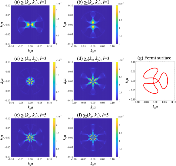
Figure S1: $\chi_{1}(\bm{\mathrm{k}})$ and $\chi_{2}(\bm{\mathrm{k}})$ for the $p$-wave ($l=1$), $f$-wave ($l=3$), and $h$-wave ($l=5$) cases. We consider $\Delta_{1}=65$ meV, $\mu=54.474$ meV, and $T=0.1$ K. (a), (b): The $p$-wave case. (c), (d): The $f$-wave case. (e), (f): The $h$-wave case. The $\chi_{1}(\bm{\mathrm{k}})$’s as functions of $\bm{\mathrm{k}}$ are plotted in (a), (c), and (e); The $\chi_{2}(\bm{\mathrm{k}})$’s as functions of $\bm{\mathrm{k}}$ are plotted in (b), (d), and (f). Only half of the $\bm{\mathrm{k}}$ points are computed. We extend the results by using $\chi_{a}(-\bm{\mathrm{k}})=\chi_{a}(\bm{\mathrm{k}})$ with $a=1,2$. (g) The Fermi surface corresponds to $\Delta_{1}=65$ meV and $\mu=54.474$ meV.

III The Kohn-Luttinger mechanism

We estimate the effective interaction strength $g_{l}$ in Eq. (3) based on a static RPA theory. The screened Coulomb interaction, $W_{\mathbf{q}}$, in the RPA theory is

$$W_{\mathbf{q}}=\frac{V_{\mathbf{q}}}{1-V_{\mathbf{q}}\chi_{0,\mathbf{q}}},$$ (S49)

where

$$V_{\mathbf{q}}=\frac{2\pi e^{2}}{\epsilon q}\tanh(qd_{M})$$ (S50)

is the bare Coulomb interaction assuming a symmetric dual metallic gates positioned at a distance $d_{M}$ from the sample. In the following calculations, we have used the dielectric constant of $\epsilon=5$ and a gate distance $d_{M}=10$ nm. In the long-wavelength limit,

$$\lim\limits_{q\rightarrow 0}V_{\mathbf{q}}=\frac{2\pi e^{2}d_{M}}{\epsilon}.$$ (S51)

In the quarter-metal parent state, one of the four spin-valley flavors remains metallic, while the other three are insulating. As a result, the static polarization function is dominated by particle-hole fluctuations within the metallic flavor, which corresponds to the $+K$ valley with spin-up electrons (as assumed in the main text). Since interband transitions have a minor impact on the metallic state, we project the interaction to the first conduction band. The resulting static polarization function is given by

$$\chi_{0,\mathbf{q}}=\frac{1}{\mathcal{A}}\sum\limits_{\mathbf{k}}\frac{n_{\rm F}(\varepsilon_{\mathbf{k}}-\mu)-n_{\rm F}(\varepsilon_{\mathbf{k}+\mathbf{q}}-\mu)}{\varepsilon_{\mathbf{k}}-\varepsilon_{\mathbf{k}+\mathbf{q}}}|\Lambda(\mathbf{k,\mathbf{q}})|^{2}.$$ (S52)

Here, $n_{\rm F}$ is the Fermi-Dirac distribution, $\mu$ is the chemical potential, $\varepsilon_{\mathbf{k}}$ is the quasiparticle eigenenergy, and $\Lambda(\mathbf{k,\mathbf{q}})$ is the overlap between wavefunctions, which sums over layers and sublattices:

$$\Lambda(\mathbf{k,\mathbf{q}})=\sum\limits_{\alpha}\phi_{\alpha}(\mathbf{k})\phi^{*}_{\alpha}(\mathbf{k}+\mathbf{q}).$$ (S53)

To estimate the effective interaction strength $g_{l}$ in Eq. (3), we approximate the screened Coulomb interaction $W_{\mathbf{q}}$ as a function of the relative angle $\theta=\phi_{\mathbf{k}^{\prime}}-\phi_{\mathbf{k}}$ between the momenta of incoming ($\mathbf{k}^{\prime}$) and outgoing ($\mathbf{k}$) Cooping pairs. We assume that $W_{\mathbf{q}}$ primarily depends on the magnitude of $\mathbf{q}=\mathbf{k}^{\prime}-\mathbf{k}$, with $|\mathbf{k}|$ and $|\mathbf{k}^{\prime}|$ being equal with a magnitude $k_{C}$:

$$q =2k_{C}\sin\theta/2,$$ (S54)

$$\theta =2\arcsin\Big{(}\frac{q}{2k_{C}}\Big{)}.$$ (S55)

Under these assumptions, $W_{\mathbf{q}}\approx W(\cos\theta)$ can be expanded in terms of Legendre polynomials,

$$W(\cos\theta)=\sum\limits_{l=0}^{\infty}W_{l}P_{l}(\cos\theta),$$ (S56)

and the effective interaction in the $l$-th angular momentum channel is

$$W_{l}=\frac{2l+1}{2}\int_{-1}^{1}W(\cos\theta)P_{l}(\cos\theta)d\cos\theta,$$ (S57)

which relates to the effective attraction in Eq. (3) by $W_{l}=-g_{l}$. Figure S2 shows the bare Coulomb potential $V_{q}$ in Eq. (S50) and the screened Coulomb potential $W_{q}$ using Eq. (S49) as a function of $q$ and $\cos\theta$, calculated for $\Delta_{1}=65$ meV, $n_{e}=0.4\times 10^{12}$ cm^-2. Both $V_{q}$ and $W_{q}$ are averaged over the angle of $\mathbf{q}$ vector. After screening, the repulsive Coulomb interaction is minimized at an intermediate value of $q$. For the case of $\Delta_{1}=65$ meV and $n_{e}=0.4\times 10^{12}$ cm^-2, the leading interaction terms are approximately:

$$\begin{split}W_{0}&=160.3\text{ meV}\cdot\text{nm}^{2},\\ W_{1}&=-131.1\text{ meV}\cdot\text{nm}^{2},\\ W_{2}&=26.6\text{ meV}\cdot\text{nm}^{2},\\ W_{3}&=-1.3\text{ meV}\cdot\text{nm}^{2},\\ W_{4}&=21.7\text{ meV}\cdot\text{nm}^{2},\\ W_{5}&=-12.2\text{ meV}\cdot\text{nm}^{2}.\\ \end{split}$$ (S58)

In this regime, the effective attraction in the $p$-wave channel is dominant. It should be noted that this estimation is based on a sparse $k$-grid with 1800 points. A denser $k$-grid or a more accurate determination of the Fermi momentum would likely improve the precision of the calculated effective interactions. To estimate the $g_{l}$ discussed in the main text, we also need to average over different $k_{C}$ and relax the equal magnitude condition for $\bm{\mathrm{k}}$ and $\bm{\mathrm{k}}^{\prime}$. Nevertheless, this crude estimation qualitatively captures the relative magnitude of interactions for different angular momentum channels. Using the minimal model discussed in the main text and set $g_{1}=-w_{1}$, a maximal $T_{c}\approx 0.2$ K is obtained, consistent with the experiment. A systematic investigation of the Kohn-Luttinger mechanism should provide a better quantitative estimate of the $T_{c}$, which we defer for future studies.

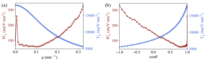
Figure S2: The bare Coulomb potential $V_{q}$ in Eq. (S50) and the screened Coulomb potential using Eq. (S49) as a function of (a) $q$ and (b) $\cos\theta$, calculated for $\Delta_{1}=65$ meV, $n_{e}=0.4\times 10^{12}$ cm^-2. Both $V_{q}$ and $W_{q}$ are averaged over the angle of $\mathbf{q}$ vector. After screening, the repulsive Coulomb is minimized at an intermediate $q$. In this calculation, the Fermi momentum is estimated to be $k_{C}\sim 0.16$ nm^-1, and we have used a sparse $k$-grid with 1800 points in the calculation of polarization function.