Benchmarking Sub-Genre Classification For Mainstage Dance Music

Abstract

Music classification, with a wide range of applications, is one of the most prominent tasks in music information retrieval. To address the absence of comprehensive datasets and high-performing methods in the classification of mainstage dance music, this work introduces a novel benchmark comprising a new dataset and a baseline. Our dataset extends the number of sub-genres to cover most recent mainstage live sets by top DJs worldwide in music festivals. A continuous soft labeling approach is employed to account for tracks that span multiple sub-genres, preserving the inherent sophistication. For the baseline, we developed deep learning models that outperform current state-of-the-art multimodel language models, which struggle to identify house music sub-genres, emphasizing the need for specialized models trained on fine-grained datasets. Our benchmark is applicable to serve for application scenarios such as music recommendation, DJ set curation, and interactive multimedia, where we also provide video demos. Our code is on https://anonymous.4open.science/r/Mainstage-EDM-Benchmark/.

Index Terms—  music datasets, deep learning, genre classification benchmark, soft labels, music visualization

1 Introduction

Being one of the most fundamental and important tasks in music information retrieval (MIR), music genre classification has mainly focused on broad genres [1, 2, 3, 4]. Despite continuous progress, existing datasets lack fine-grained labels that can capture the nuances within electronic dance music (EDM), and with 0/1 labels, they hardly manifest the category overlap in EDM data. Moreover, current universal models have subpar performance in specific tasks [5, 6]. The limitations are evident in the contexts of mainstage DJ sets, where tracks usually fall into sub-genres within the broad category of house music. Hence, the unique challenges presented by EDM need specialized datasets and algorithms tailored to its structural characteristics and its complexity with regard to production techniques.

To address this gap, we introduce a new benchmark specifically targeting at the classification of house music sub-genres. A dataset is designed to provide annotations from a list of 8 sub-genres. Unlike existing dataset HouseX [7], we introduce soft labeling instead of 0/1 categorical labeling to provide detailed and nuanced representation of the music. In addition, a baseline model is presented using spectral features [8, 9], building a foundation for future research in dance music genre classification. Furthermore, an application of our models in automated music visualization is prototyped to enhance visual experiences.

Overall, this work aims to advance MIR for mainstage house music by offering a more comprehensive dataset and efficient baseline. Our key contributions are:

1. An improved annotation paradigm and a larger dataset.

2. A strong baseline for this dataset.

3. A VFX automation demo driven by trained models.

The rest sections are as follows: Sec. 2 reviews related work, Sec. 3 outlines our methodology, Sec. 4 presents our results, and Sec. 5 discusses potential applications, with conclusions in Sec. 6.

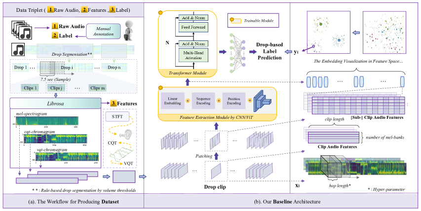
Fig. 1: Pipeline structure

2 Related Work

Traditional music genre datasets, like GTZAN [1], FMA [2] and MSD [10], often focus on broad genres like pop, country, and rock. The HouseX dataset [7] advanced classification on EDM but faced challenges like limited category richness and scale. In addition, previous works tackling drop detection [11, 12, 13] also highlight the emerging research interest in MIR for EDM. Alongside traditional deep learning methods, recent progress on multimodel large language models (MLLMs) like the Qwen-Audio series [5, 14] could also be used to classify generic audio.

This work presents a new dataset expanding on [7], featuring 1000+ tracks from record labels and doubling the number of sub-genres. We use soft labeling to capture tracks with multiple sub-genre traits. Our architecture employs convolutional neural networks (CNNs) [15, 16, 17] and vision transformers (ViTs) [18] to extract features with a sliding window, followed by some transformer encoder layers to predict the target distribution. These models significantly outperform the Qwen-Audio series, the state-of-the-art open-source LLMs that take audio as direct input.

3 Methodology

This section discusses our methodology, from the collection and annotation of the dataset, to the training of the model. Fig. 1 illustrates the pipeline. For simplicity, we refer to “sub-genres” of house music as “genres” from here unless otherwise specified. Statistics of our dataset is shown in Tab. 1. In the table, the first part lists the number of clips for the 8 genres in the training set and the validation set, while the second part gives some other general statistics.

3.1 Dataset

Our data preparation stage involves collection, annotation, and extraction of musical excerpts. The input data are represented as triplets, each comprising the raw audio ($X_{\text{raw}}$), its extracted acoustic features ($X_{\text{feat}}$), and a corresponding label ($Y$), as illustrated by numbers from 1 to 3 in Fig. 1.

Our dataset comprises over 1,000 selected tracks sourced from renowned international record companies. These tracks are stored as uncompressed raw audio ($X_{\text{raw}}$). For each track, we only consider the drop, which is the most representative segment of the style. To identify these segments, we detect excerpts where the volume consistently remains above a threshold ($V_{\text{thres}}=V_{\text{max}}-V_{\text{margin}}$), where $V_{\text{max}}$ denotes the maximum volume within the audio. Note that before detection, some rule-based smoothing process is applied to mitigate loudness fluctuations. After identifying the segments that meet the aforementioned criteria, several 7.5-second clips (around 4 bars) are randomly sampled from each segment, ensuring a comprehensive representation of the track.

Subsequently, feature extraction is performed on each clip. Using Librosa [19], we compute: mel-spectrograms ($X_{\text{mel}}$), CQT-chromagrams ($X_{\text{cqt}}$), VQT-chromagrams ($X_{\text{vqt}}$), which are then stacked to produce the final audio feature matrix ($X_{\text{feat}}$).

All tracks in the dataset are manually annotated with a total of eight distinct labels. The first four labels align with those previously defined by the HouseX dataset [7]. To improve classification granularity to a level suitable for covering most contemporary mainstage live sets, we introduce four additional genres. Recognizing that certain tracks may exhibit characteristics of multiple genres, we employ soft labeling techniques to add more information to our labels. We also show that soft labeling gives better performance than hard 0/1 labels in Sec. 4.

Table 1: Dataset Statistics

Genre	# of Clips
	Train.	Val.
Progressive House	1215	344
Future House	1192	348
Bass House	1102	120
Tech House	643	200
Deep House	591	116
Bigroom	774	284
Future Rave	920	108
Slap House	667	232
Total	7104	1752
# of Tracks (Train. & Val.)	1035
Sample Rate	44100 Hz
BPM Range	115-130

3.2 Model

Given a dataset of audio features $\{X_{\text{feat}}^{i}\}_{i=1}^{N}$ with corresponding soft labels $p(y_{i}|X_{\text{feat}}^{i})$ that represent probability distributions over possible genres, our objective is to train a neural network, parameterized by $\theta$, to predict genre distributions $q_{\theta}(y_{i}|X_{\text{feat}}^{i})$ that closely match these soft labels.

To achieve this goal, we minimize the Kullback-Leibler (KL) divergence between the true distribution $p(y_{i}|X_{\text{feat}}^{i})$ and the predicted distribution $q_{\theta}(y_{i}|X_{\text{feat}}^{i})$:

$$\text{KL}(p\parallel q_{\theta})=\sum_{i=1}^{N}\sum_{y_{i}\in\mathcal{Y}}p(y_{i}|X_{\text{feat}}^{i})\log\left(\frac{p(y_{i}|X_{\text{feat}}^{i})}{q_{\theta}(y_{i}|X_{\text{feat}}^{i})}\right).$$

Discarding the part that does not depend on $\theta$, this is equivalent to minimizing the cross-entropy loss:

$$\mathcal{L}(\theta)=-\sum_{i=1}^{N}\sum_{y_{i}\in\mathcal{Y}}p(y_{i}|X_{\text{feat}}^{i})\log\left(q_{\theta}(y_{i}|X_{\text{feat}}^{i})\right).$$

The architecture of network $\theta$ is inspired by AST (audio spectrogram transformer) [20] trained on the AudioSet [21]. As shown in column (b) in Fig. 1, we derive a sequence of overlapping patches $\{X_{\text{feat}}^{i,j}\}_{j=1}^{M}$ from each acoustic feature matrix $X_{\text{feat}}^{i}$, where $X_{\text{feat}}^{i,j}$ is square with shape ($3\times 224\times 224$). Then each square feature patch is fed into a vision encoder, which essentially consists of conventional architectures used for image classification [15, 16, 17, 18]. The output for the sequence of input feature patches is a corresponding sequence of embeddings $\{Z_{\text{emb}}^{i,j}\}_{j=1}^{M}$. Positional encodings are then added to this sequence of embeddings, which are subsequently passed through several stacked transformer [22] encoder layers. The first (on the $seq\_len$ axis) output from this transformer is finally fed into a linear layer to get the predicted distribution.

Compared with the previous architecture in HouseX [7], which is solely an image classifier, we convert the raw feature matrix into a sequence of patches because the clip length has quadrupled. In fact, keep resizing the feature matrix into squares in a brute-force manner would lead to sever information loss on the temporal axis, which is crucial for characterizing genres like future house that contain very fragmentary music notes or samples.

4 Results

This section presents the experiment results alongside our interpretations and findings. Tab. 2 provides numerical details and Fig. 2 shows the final embedding space after feature reduction by PCA, t-SNE [23] and UMAP [24].

Four popular CNN/ViT architectures (with comparable number of parameters) serve as the feature extractor. Experiments show that all of these settings outperform Qwen2-Audio, with or without prompt on background knowledge. Again, our purpose is to justify the necessity of building specific dataset rather than “beat” MLLMs. In other words, MLLMs are quite likely to distinguish among EDM sub-genres when provided with proper fine-tuning data; otherwise, they struggle to align textual background information with domain-specific audio features. In addition, models trained on soft labels perform uniformly better than those trained from (sharpened) 0/1 labels, which supports our claim that soft labeling provides richer information of the tracks. Moreover, models trained on composite data with chromagrams fail to surpass those trained solely on mel-spectrogram. We attribute this phenomenon to the domain gap between the RGB channels and the mel-CQT-VQT space. Future work on architectures using such composite data could focus on improving feature fusion techniques to achieve better results.

We also extracted the embeddings before the final linear layer and visualized them with dimension reduction techniques. The figures indicate that progressive house, bigroom and slap house are relatively well-separated, aligning with our annotations where most non-0/1 labels involve other genres.

Table 2: Experiment Results on the Validation Set

Architecture								Precision$\star$				Recall$\star$	F1$\star$
chroma info$\dagger$	w		w/o		w		w/o		w		w/o
label setup$\ddagger$	hard	soft	hard	soft	hard	soft	hard	soft	hard	soft	hard	soft
ours (vit_b_16)	$0.077$	$0.039$	$0.039$	$0.039$	$0.224$	$0.199$	$0.199$	$0.199$	$0.109$	$0.066$	$0.066$	$0.066$
ours (vgg11_bn)	$0.746$	$0.751$	$0.739$	$0.765$	$0.716$	$0.748$	$0.735$	$0.757$	$0.722$	$0.747$	$0.731$	$0.756$
ours (densenet201)	$0.730$	$0.767$	$0.786$	0.790	$0.712$	$0.749$	$0.752$	$0.743$	$0.716$	$0.741$	$0.757$	$0.751$
ours (resnet152)	$0.760$	$0.761$	$0.776$	$0.780$	$0.720$	$0.737$	$0.748$	0.761	$0.718$	$0.744$	$0.756$	0.764
Qwen-Audio (full-prompt)	0.122				0.099				0.037
Qwen-Audio (min-prompt)	0.109				0.170				0.116
Qwen2-Audio (full-prompt)	0.202				0.129				0.031
Qwen2-Audio (min-prompt)	0.165				0.104				0.029

• The 3 metrics here are weighted averages across all 8 genres.

• This row indicates whether we include chromagrams in the data representation.

• This row indicates whether a hard 0/1 labeling or a soft labeling approach is used in the data representation.

• “Full-prompt” include GPT-4o-generated documentation and human expertise in the text prompt, while “min-prompt” only gives the question without any background information.

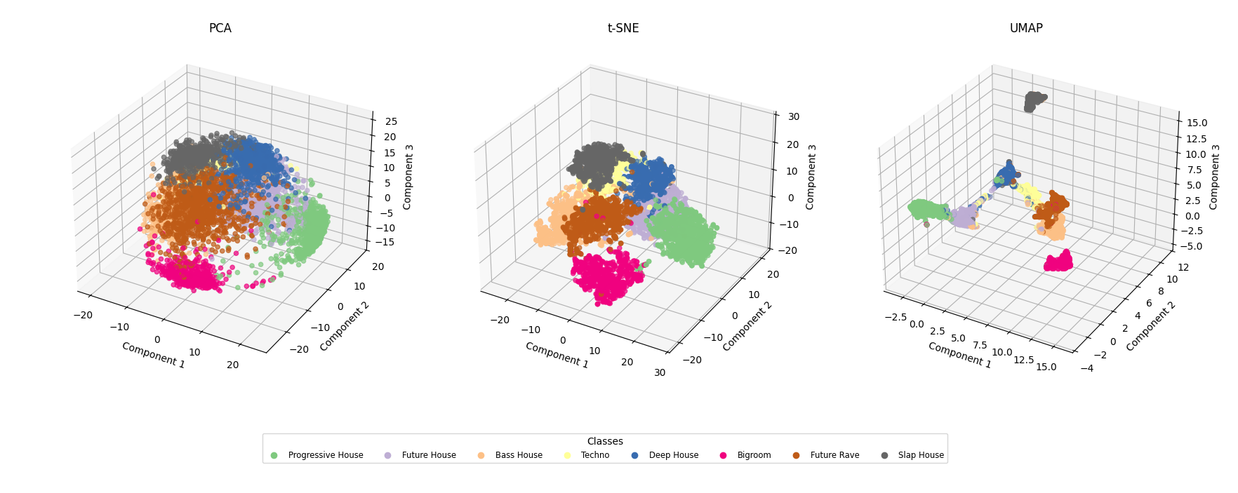
Fig. 2: 3D Feature Visualization of the Training Set

Table 3: Determinants of House Music Sub-genres

Genre	Lead Inst.	Chord Inst.	Bass Inst.	Groove	Rhythm	Distortion	Organicity
Progressive House	✓	✓	✓	4-5	1-3	1-2	3-5
Future House	✓	$\sim$	✓	3-4	4-5	3-4	1-3
Bass House	✓	✗	✓	2-4	3-4	4-5	1-2
Tech House	✗	✗	✓	3-5	3-4	2-4	1-3
Deep House	✓	$\sim$	✓	2-3	1-2	1-2	2-4
Bigroom	✓	✗	✗	1-2	1-3	4-5	1-2
Future Rave	✓	✗	✓	4-5	3-5	2-4	1-2
Slap House	✓	✗	✓	3-4	3-5	1-3	1-2

• ✓ denotes “yes”, ✗ denotes “no” and $\sim$ denotes “uncertain”, which could be either yes or no depending on the track.

5 Applications

We propose some real-world scenarios for such classification algorithm. A straightforward application is music recommendation system tailored for listeners with specific preferences on certain sub-genres. Besides, this algorithm can boost productivity in multimedia contexts, such as automated MV generation and visuals generation given certain pre-defined rules [7]. For illustrative purposes, we prototyped a visual automation system simulated in Blender 3D.

6 Conclusion

We developed a comprehensive house music classification benchmark to address the limitations of existing datasets, such as limited sub-genre representation and inter-class overlaps. Our dataset employs continuous soft labeling to better capture track characteristics. Our proposed baseline methods outperform current MLLMs on this classification task, highlighting the significance of specialized datasets.

Future work will further scale up the dataset to better utilize the CQT and VQT feature spaces. Since labeling large datasets is impractical for the machine learning community alone, a collaborative approach with production experts is recommended. Future research should also extend beyond sub-genre classification to encompass timbral and rhythmic characteristics. Additionally, we aim to develop a Multimodal Large Language Model (MLLM) capable of captioning EDM tracks with descriptive attributes to enhance downstream applications.

Appendix A: Classification Protocols

Due to space constraints, please find the definitions of the determinants we used in Tab. 3 in the “misc” subfolder of our code. Numerical scores are quantized from averages given by human music producers. We also provide qualitative descriptions of the 8 genres in the same folder. Note that the values of soft labels are not absolute per se. Even for professionals, one track can be interpreted in multiple ways. Soft labels are utilized to indicate “Track $X$ is genre $A$ but also expresses some traits of genre $B$”, for example, so more information is contained in the label.

Appendix B: Experiment Settings

At least 24G GPU memory is required to complete one run with a batch size of 4. We assign one NVIDIA RTX A6000 GPU to each data setting (whether to use chromagram and whether to use soft labels). Completing 5 epochs for all 4 architectures in a single setting requires 1 day.

References

- [1] George Tzanetakis et al., “Automatic musical genre classification of audio signals,” 2001.
- [2] Michaël Defferrard et al., “FMA: A dataset for music analysis,” in 18th International Society for Music Information Retrieval Conference (ISMIR), 2017.
- [3] Michaël Defferrard et al., “Learning to recognize musical genre from audio,” in The 2018 Web Conference Companion. 2018, ACM Press.
- [4] Monan Zhou et al., “CCmusic: an open and diverse database for chinese and general music information retrieval research,” mar 2024.
- [5] Yunfei Chu et al., “Qwen-audio: Advancing universal audio understanding via unified large-scale audio-language models,” arXiv preprint arXiv:2311.07919, 2023.
- [6] Yunfei Chu et al., “Qwen2-audio technical report,” 2024.
- [7] Xinyu Li, “HouseX: A fine-grained house music dataset and its potential in the music industry,” in 2022 Asia-Pacific Signal and Information Processing Association Annual Summit and Conference (APSIPA ASC), 2022, pp. 335–341.
- [8] Christian Schörkhuber, “Constant-q transform toolbox for music processing,” 2010.
- [9] Christian Schörkhuber et al., “A matlab toolbox for efficient perfect reconstruction time-frequency transforms with log-frequency resolution,” in Semantic Audio, 2014.
- [10] Thierry Bertin-Mahieux et al., “The million song dataset,” in Proceedings of the 12th International Society for Music Information Retrieval Conference, 2011, pp. 591–596.
- [11] Giulia Argüello et al., “Cue point estimation using object detection,” 2024.
- [12] Karthik Yadati et al., “Detecting drops in electronic dance music: Content based approaches to a socially significant music event,” in Proceedings of the 15th International Society for Music Information Retrieval Conference, ISMIR 2014, Taipei, Taiwan, October 27-31, 2014, Hsin-Min Wang, Yi-Hsuan Yang, and Jin Ha Lee, Eds., 2014, pp. 143–148.
- [13] Yu-Siang Huang et al., “Pop music highlighter: Marking the emotion keypoints,” Transactions of the International Society for Music Information Retrieval, vol. 1, no. 1, pp. 68–78, 2018.
- [14] Yunfei Chu et al., “Qwen2-audio technical report,” arXiv preprint arXiv:2407.10759, 2024.
- [15] Kaiming He et al., “Deep residual learning for image recognition,” 2016 IEEE Conference on Computer Vision and Pattern Recognition (CVPR), pp. 770–778, 2015.
- [16] Gao Huang et al., “Densely connected convolutional networks,” 2017 IEEE Conference on Computer Vision and Pattern Recognition (CVPR), pp. 2261–2269, 2016.
- [17] Karen Simonyan et al., “Very deep convolutional networks for large-scale image recognition,” CoRR, vol. abs/1409.1556, 2014.
- [18] Alexey Dosovitskiy et al., “An image is worth 16x16 words: Transformers for image recognition at scale,” ArXiv, vol. abs/2010.11929, 2020.
- [19] Brian McFee et al., “librosa: Audio and music signal analysis in python,” in Proceedings of the 14th python in science conference, 2015, vol. 8.
- [20] Yuan Gong et al., “AST: Audio Spectrogram Transformer,” in Proc. Interspeech 2021, 2021, pp. 571–575.
- [21] Jort F. Gemmeke et al., “Audio set: An ontology and human-labeled dataset for audio events,” in 2017 IEEE International Conference on Acoustics, Speech and Signal Processing (ICASSP), 2017, pp. 776–780.
- [22] Ashish Vaswani et al., “Attention is all you need,” in Proceedings of the 31st International Conference on Neural Information Processing Systems, Red Hook, NY, USA, 2017, NIPS’17, p. 6000–6010, Curran Associates Inc.
- [23] Laurens van der Maaten et al., “Visualizing data using t-sne,” Journal of Machine Learning Research, vol. 9, no. 86, pp. 2579–2605, 2008.
- [24] Leland McInnes et al., “Umap: Uniform manifold approximation and projection for dimension reduction,” 2020.