Entanglement transfer during quantum frequency conversion
in gas-filled hollow-core fibers

Abstract

Quantum transduction is essential for future hybrid quantum networks, connecting devices across different spectral ranges. In this regard, molecular modulation in hollow-core fibers has proven to be exceptional for efficient frequency conversion. However, insights on this conversion method for quantum light have remained elusive beyond standard semiclassical models. This Letter introduces a framework to describe the quantum dynamics of both molecules and photons in agreement with recent experiments and capable of unveiling the ability of molecular modulation to preserve entanglement.

Understanding light-matter interactions at the quantum level lies at the core of the recent developments in quantum technologies Tavis1968 ; Aspelmeyer2014 ; Schmidt2016 ; Blais2021 that are behind sophisticated systems such as the future hybrid quantum networks Kimble2008 . These systems comprise multiple devices such as quantum light sources and memories, fiber transmission lines, etc., which operate across different spectral regions of the optical domain, in sharp contrast to e.g. the microwave superconducting circuits employed in state-of-art quantum computers Girvin2014 ; Gu2017 . Thus, efficient frequency transduction of quantum light states between disparate domains  Li2004 ; Lauk2020 is essential to bridge the operational gaps between nodes Awschalom2021 . While several different approaches to tackle this challenge have been proposed and demonstrated Fan2016 ; Bonsma2022 , molecular modulation in hollow-core anti-resonant fibers (ARFs) filled with gas Russell2014 ; Numkam2023 has recently stood out owing to its near-unity efficiency and exquisite preservation of non-classical correlations Tyumenev2022 . This is facilitated by the tight light-matter confinement in the core Russell2014 , ultralow attenuation over a broad bandwidth Numkam2023 and pressure-adjustable optical properties Bauerschmidt2015 , which make ARFs excellent vehicles for light-based quantum applications Finger2015 ; Antesberger2024 .

On the other hand, in molecular modulation Liang2000 ; Weber2012 at the single-photon level, a quantum light state scatters off the molecular coherence waves pre-excited via stimulated Raman scattering (SRS) in the ARF core, changing its frequency by the appropriate Raman shift without threshold. The corresponding state can be controllably up- or down-converted provided specific phase-matching conditions are fulfilled, which in the case of gas-filled ARFs is achieved by leveraging the fiber dispersion Mridha2019 .

Despite the great potential of ARF-based molecular modulation for quantum transduction Tyumenev2022 , it still remains unclear whether intrinsic quantum properties such as entanglement can be transferred with high fidelity from the original to the target states during the conversion process, a question that cannot be answered using the widely-employed Maxwell-Bloch formalism Raymer1985 ; Raymer1990 . The main reason is its classical treatment of the light fields, although it has been applied to the modelling of certain quantum optical phenomena like photon absorption and emission in weakly-excited atomic clouds Svidzinsky2015 . Therefore, apart from some recent efforts in this direction Wang2023 , a rigorous and accurate description of quantum light-quantum matter interactions in ARF-based frequency conversion down to single-photon limit has, to our best knowledge, so far remained elusive.

In this Letter, we present a quantum Hamiltonian able to describe both the coherence buildup in a molecular gas through SRS, as well as the subsequent thresholdless frequency-conversion process at the single-photon level. In particular, considering the experimental scenario reported in Ref. Tyumenev2022 , we are able to characterize the state of the molecules and predict a complete transfer of entanglement between one of the modes of a Bell state and its corresponding frequency-converted counterpart. Our model can be applied to both confined and free-space geometries and reduces to the semiclassical Maxwell-Bloch formalism Raymer1990 for strong light fields. We expect this general theoretical framework to aid the design, optimization and interpretation of future experiments in light-based quantum technologies using ARFs and their subsequent applications.

The process we want to describe is molecular modulation assisted by SRS Harris1998 ; Nazarkin1999 . We consider two-level molecules in general and, inspired by the experimental results, we focus on the Q$(1)$ vibrational transition of hydrogen as a good two-level approximation. This transition is dipole-forbidden, and therefore needs a two-photon process such as Raman scattering to occur (depicted in Fig. 1).

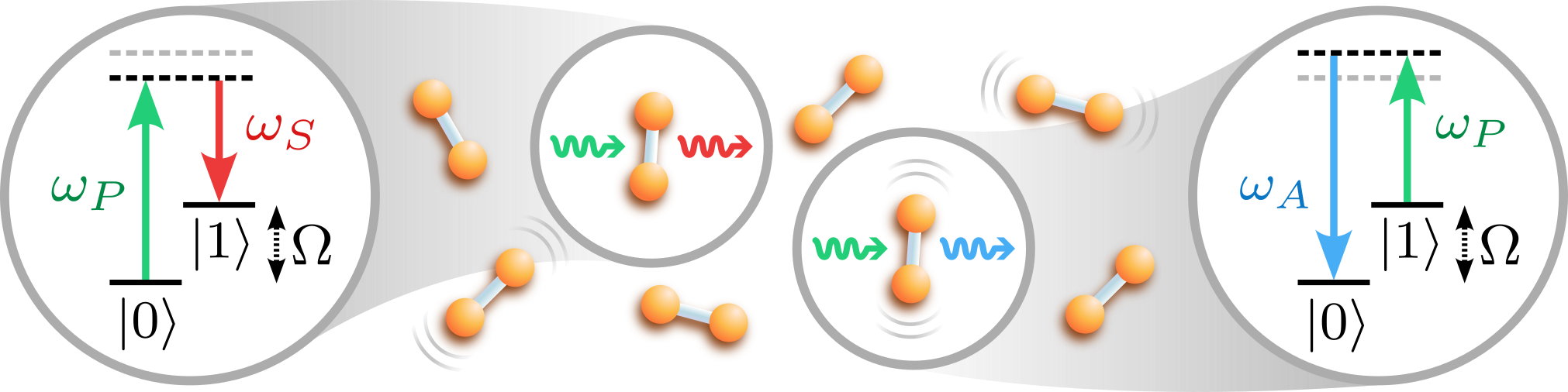
Figure 1: Illustration of Raman scattering in a molecular diatomic gas. (Left) A photon with pump frequency $\omega_{P}$ is inelastically scattered by a molecule in the vibrational ground state $|0\rangle$. As a result of the interaction, the molecule gains an energy defined by the Raman frequency $\Omega$, transitioning into the excited vibrational state $|1\rangle$. Meanwhile, the scattered photon ends with Stokes frequency $\omega_{S}=\omega_{P}-\Omega$. (Right) The inverse process is also represented, involving the de-excitation of molecules via the inelastic scattering of a pump photon into the anti-Stokes frequency $\omega_{A}=\omega_{P}+\Omega$. Dashed lines indicate off-resonant energy levels.

In this process, the pump photons launched in the fundamental core mode of the H₂-filled ARF (illustrated in Fig. 2) are scattered into the Stokes or anti-Stokes frequencies depending on whether they excite or de-excite the molecules, respectively. These transitions are illustrated in Fig. 1, where $\omega_{P}$, $\omega_{S}$, and $\omega_{A}$ are the pump, Stokes, and anti-Stokes angular frequencies, and $\Omega$ represents the Raman shift, such that $\omega_{S}=\omega_{P}-\Omega$ and $\omega_{A}=\omega_{P}+\Omega$. For the H₂ gas case, $\Omega/2\pi\approx 125\text{ THz}$ Veirs1987 , the largest molecular shift in nature. Without loss of generality, the light is linearly polarized in our analysis, and therefore rotational states are highly disfavored. Furthermore, hereafter we will consider all the optical frequencies involved in the dynamics contained in the fundamental transmission band of the ARF, i.e. spectrally away from loss-inducing resonances with modes localized in the cladding elements Numkam2023 .

The quantum Hamiltonian describing the pump, Stokes, and anti-Stokes modes of the electric field interacting with a single molecule is expressed as $H=H_{0}+V$ Scully1997 ; Begzjav2021 . On the one hand, we have the unperturbed part of the Hamiltonian $H_{0}$, defined as

$$H_{0}/\hbar=\omega_{0}|0\rangle\langle 0|+\omega_{1}|1\rangle\langle 1|+\sum_{i=2}^{\infty}\omega_{i}|i\rangle\langle i|+\sum_{l}\omega_{l}a^{\dagger}_{l}a_{l},$$ (1)

where $l\in\{\text{P, S, A}\}$ labels the operators associated to the pump, Stokes, and anti-Stokes modes, respectively. The quantity $\hbar\omega_{i}$ is the energy associated to the vibrational states $|i\rangle$ of the molecule, and $\omega_{l}$ is the frequency associated to mode $l$. On the other hand, the interaction part of the Hamiltonian, $V$, is given by

$$V=\sum_{i,j}\sum_{l}g_{i,j}^{l}|i\rangle\langle j|\left(a_{l}e^{i\beta_{l}z}-a_{l}^{\dagger}e^{-i\beta_{l}z}\right),$$ (2)

where $g_{i,j}^{l}$ is the coupling strength between levels $|i\rangle$ and $|j\rangle$ via bosonic mode $l$, and $\beta_{l}$ is the propagation constant for mode $l$. Let us now eliminate the higher energy levels, i.e. levels with $i>1$, to obtain an effective Hamiltonian describing the interaction of the pump, Stokes, anti-Stokes modes, with the molecule. In order to do this, we go to an interaction picture with respect to $H_{0}$ and perform a rotating-wave approximation, keeping only the static terms up to second order in the coupling strength. That is, by assuming that $g_{i,j}^{l}\sqrt{n_{l}}\ll\hbar|\omega_{i}-\omega_{j}\pm\omega_{l}|$, with $n_{l}$ the number of photons in the mode $l$, we keep only the resonant terms. The only resonances we can identify in this system are $\omega_{P}-\omega_{S}=\Omega=\omega_{A}-\omega_{P}$, with $\Omega\equiv\omega_{1}-\omega_{0}$. Extending this approach to a system with $N$ molecules, we find the effective Hamiltonian SM

$$H_{\text{eff}} = \hbar\Omega J_{z}+\hbar\sum_{l}\left(\omega_{l}+\Delta_{l}^{+}\right)a^{\dagger}_{l}a_{l}+2\hbar\sum_{l}\Delta_{l}^{-}a^{\dagger}_{l}a_{l}J_{z}$$ (3)

$$+ \hbar\left(G_{S}e^{i\Delta\beta z}a_{P}a^{\dagger}_{S}+G_{A}e^{i\Delta\beta^{\prime}z}a^{\dagger}_{P}a_{A}\right)J^{+}$$

$$+ \hbar\left(G_{S}^{*}e^{-i\Delta\beta z}a^{\dagger}_{P}a_{S}+G_{A}^{*}e^{-i\Delta\beta^{\prime}z}a_{P}a^{\dagger}_{A}\right)J^{-},$$

where $G_{S(A)}$ is the interaction strength between pump, (anti-)Stokes, and the molecules, $\Delta_{l}^{\pm}$ represent the Stark shifts, and $\Delta\beta\equiv\beta_{P}-\beta_{S}$ and $\Delta\beta^{\prime}\equiv\beta_{A}-\beta_{P}$. The global spin operators are defined through the $1/2$-spin operators as $J_{z}=\oplus_{l=1}^{N}\sigma^{z}_{l}/2$ and $J^{\pm}=\oplus_{l=1}^{N}\sigma^{\pm}_{l}$, with $\sigma^{z}=|1\rangle\langle 1|-|0\rangle\langle 0|$, $\sigma^{+}=|1\rangle\langle 0|$, and $\sigma^{-}=|0\rangle\langle 1|$. They satisfy $[J_{z},J^{\pm}]=\pm J^{\pm}$ and $[J^{+},J^{-}]=2J_{z}$ and, as operators, they act on global spin states of the form $\left|{\bf N/2},m_{z}\right\rangle$, with $m_{z}\in\{-N/2,\ldots,N/2\}$. Note that these operators treat the molecules as an ensemble of two-level systems and they are not representing actual angular momentum of the molecules or light polarization.

In Ref. Tyumenev2022 , the excitation of molecular coherence, that manifests itself as a synchronous oscillation of the gaseous core (see Fig. 2), was achieved using nanosecond-long pump pulses with 115 µJ energy. This means that the initial state of the pump can be considered as a coherent state with $\alpha_{P}\approx 2.48\times 10^{7}$, enabling a few approximations that simplify Eq. (3).

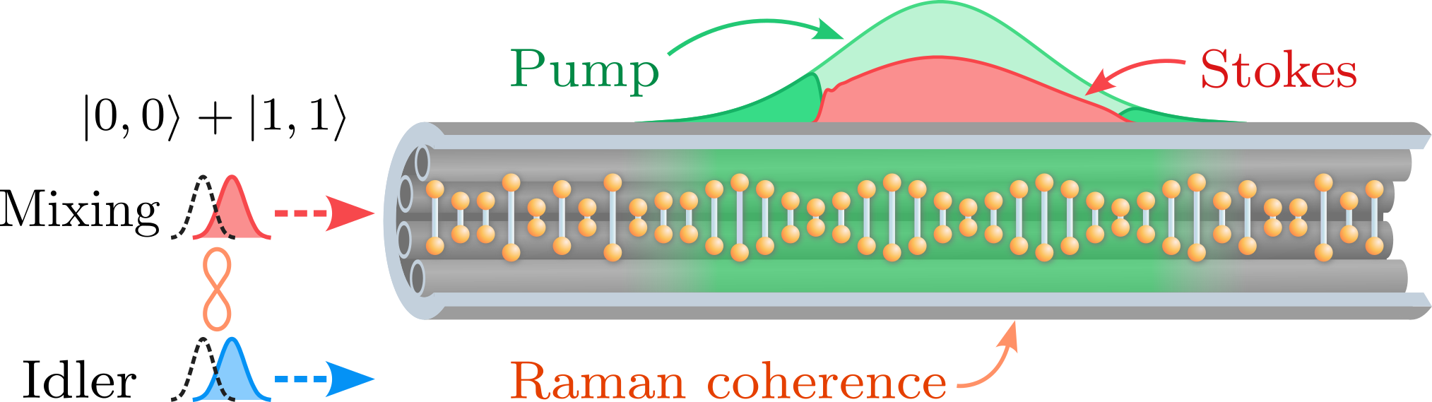
Figure 2: Schematic representation of the experimental layout considered. A pump beam generates Raman vibrational excitations in the gas molecules, preparing them in a coherent and synchronized vibrational motion. During this process, the pump is depleted into the Stokes frequency, as depicted in the figure. The mixing signal simultaneously propagating with the pump perceives the molecular coherence wave and it is scattered to a higher frequency.

Firstly, the annihilation of pump photons leads to the generation of intense laser radiation in the Stokes mode along the fiber length Benabid2002 . Therefore, we may consider a semiclassical approximation, replacing the operators in both the pump and the Stokes modes by classical variables $a_{P}\rightarrow\alpha_{P}$ and $a_{S}\rightarrow\alpha_{S}$ in Eq. (3). Additionally, since the majority of molecules remain in their ground state, the population of the anti-Stokes mode is usually negligible in this process, so we will discard it in our treatment. Finally, we consider that the Stark shifts are also negligible, $\Delta_{P}^{\pm}=\Delta_{S}^{\pm}\approx 0$. Before performing the semiclassical approximation, in order to avoid oscillations with $\Omega$ in the expectation values, we transform the Hamiltonian into an interaction picture with respect to $\Omega J_{z}+\omega_{P}a_{P}^{\dagger}a_{P}+\omega_{S}a_{S}^{\dagger}a_{S}$, obtaining

$$H_{\alpha}^{I}=\hbar\left(G_{S}e^{i\Delta\beta z}\alpha_{P}\alpha_{S}^{*}J^{+}+G_{S}^{*}e^{-i\Delta\beta z}\alpha_{P}^{*}\alpha_{S}J^{-}\right).$$ (4)

By evolving the initial state of the molecules $\left|{\bf\frac{N}{2}},-\frac{N}{2}+n\right\rangle$, which corresponds to all molecules in the ground state, under this Hamiltonian for a time $t$, we find the state in the interaction picture SM

$$|s\rangle=\left(\frac{e^{-i\Omega t}}{1+|s|^{2}}\right)^{\frac{N}{2}}\sum_{n=0}^{N}\begin{pmatrix}N\\ n\end{pmatrix}^{1/2}s^{n}\left|{\bf\frac{N}{2}},-\frac{N}{2}+n\right\rangle.$$ (5)

Here, we have $s=e^{i\left(\Delta\beta z-\frac{\pi}{2}\right)}\tan\left(G_{S}\alpha_{P}\alpha_{S}t\right)$, where we have assumed that $G_{S}$, $\alpha_{P}$, and $\alpha_{S}$ are real. Interestingly, this state has the functional form of a spin coherent or Bloch state Arecchi1972 .

The emergence of vibrational coherence in the molecular gas, highlighted in green inside the fiber at Fig. 2, originates from the beating between the pump and Stokes fields Mridha2019 ; Raymer1990 . As the amplitude of the coherence wave rises, the pump starts to suffer depletion and the Stokes starts to be amplified. As the depletion continues, the beating between the fields becomes weaker, preventing the generation of new coherence. Meanwhile, the existing coherence wave fades away due to collisional dephasing on a time scale $T_{2}$. Hence, the excited molecular coherence is harvested, within its lifetime, for frequency conversion of an arbitrary mixing signal. Unlike SRS, this frequency conversion process is thresholdless and hence, it can be applied to a single photon. Additionally, the phase-matching conditions governing the feasibility of frequency conversion of the mixing signal are highly influenced by the dispersion contributions from both the gas and the geometry of the waveguide Mridha2019 . In a nutshell, if the difference in the propagation constants of the ARF modes at the original and converted photon frequencies matches the propagation constant of the molecular coherence wave (given by the difference between those of the pump and Stokes fields), energy will be efficiently exchanged during the scattering event, resulting in a modification of the photon frequency according to the molecular Raman shift.

In the following, let us use the developed model to analyze the process of frequency conversion in one of the frequency modes of a maximally-entangled Bell state representing the mixing signal. Indeed, we will convert the mixing mode by launching it simultaneously with the pump beam, while the idler mode remains unperturbed outside of the fiber, and observe the entanglement dynamics between the idler and the mixing and up-converted modes. Considering the experimental conditions of Ref. Tyumenev2022 , the system undergoes a phase-matched transition between a mixing frequency of $\approx 210$ THz (1425 nm in wavelength) and an up-converted frequency of $\approx 335$ THz (895 nm). Even though this is not strictly a Raman transition, it can be described using a Hamiltonian with the same structure as in Eq. (3). This time, the terms describing the mixing to up-converted interaction mimic those of the pump to anti-Stokes, but with the appropriate parameters.

While the idler and the mixing frequency modes are initially prepared in a Bell state, the up-converted mode is not populated; therefore, the initial state is simply $(|0,0,0\rangle+|1,1,0\rangle)/\sqrt{2}$. This notation represents, from left to right and separated by commas, the number of photons in the idler, mixing, and up-converted modes, respectively. Since we typically have a large number of molecules ($\sim 10^{18}$), the state of the molecular ensemble will not change significantly due to the introduction of a single excitation into the system. Thus, in the Hamiltonian characterizing the frequency-conversion process, we replace the global spin operators by their expectation values over the spin coherent state in Eq. (5). That is, we replace $J^{+}\rightarrow\xi^{*}$ and $J^{-}\rightarrow\xi$, with $\xi=\langle s|J^{-}|s\rangle=(N/2)\exp[i\left(\Delta\beta z-\pi/2\right)]\sin\left(2G_{S}\alpha_{P}\alpha_{S}t\right)$. Before, let us transform the Hamiltonian into an interaction picture again with respect to $\Omega J_{z}+\omega_{M}a_{M}^{\dagger}a_{M}+\omega_{U}a_{U}^{\dagger}a_{U}$. Then, the resulting Hamiltonian is

$$H_{\xi}^{I} = \hbar G_{U}\Big{(}\xi^{*}e^{i[(\Omega+\omega_{M}-\omega_{U})t-(\beta_{M}-\beta_{U})z]}a_{M}^{\dagger}a_{U}$$

$$+ \xi e^{-i[(\Omega+\omega_{M}-\omega_{U})t-(\beta_{M}-\beta_{U})z]}a_{M}a_{U}^{\dagger}\Big{)},$$

where $G_{U}$ represents the interaction strength between the mixing, the up-converted, and the molecules, and is supposed to be real. Assuming resonance and phase-matching conditions, that are experimentally achievable, we can write $\omega_{U}-\omega_{M}=\Omega$ and $\beta_{U}-\beta_{M}=\Delta\beta$, respectively. The Hamiltonian in Eq. (Entanglement transfer during quantum frequency conversion in gas-filled hollow-core fibers) describes beamsplitter-like dynamics with a time-dependent reflectivity $\sin^{2}G_{U}|\xi|t$, and thus the evolution of a single-photon frequency state can easily be computed. In this framework, the resulting equations for the evolution of the mixing, $N_{M}$, and the up-converted, $N_{U}$, photon numbers are as follows:

$$N_{M} = \frac{1}{2}\cos^{2}G_{U}|\xi|t,$$ (7)

$$N_{U} = \frac{1}{2}\sin^{2}G_{U}|\xi|t.$$ (8)

Meanwhile, we also study the dynamics of entanglement between the mixing and the up-converted frequency modes through the concurrence Wootters1998 , an entanglement monotone used for bipartite mixed states. This is an appropriate choice in this case since we have entanglement between the idler and the mixing modes, but also between the idler and up-converted modes. Furthermore, the concurrence completely characterizes the entanglement of formation Hill1997 for a pair of two-level systems. In our case, we find that the idler-mixing and the idler-up-converted concurrences are SM

$$\mathcal{C}_{\text{I-M}} = \Big{|}\cos G_{U}|\xi|t\Big{|},$$ (9)

$$\mathcal{C}_{\text{I-U}} = \Big{|}\sin G_{U}|\xi|t\Big{|}.$$ (10)

Notice how entanglement transfer between mixing and up-converted modes is closely related to the evolution of the number of photons in each mode, such that frequency conversion leads to entanglement transfer. The time parameter $t$ here is considered to be related to the propagation distance $z$ inside the fiber used in Ref. Tyumenev2022 , $z=ct$. This is used to represent the evolution of the photon numbers and the concurrences in Fig. 3, where the explicit time dependence of $\alpha_{P}$ and $\alpha_{S}$ has been considered SM . These coefficients are obtained by numerically solving the semiclassical Maxwell-Bloch equations of motion Raymer1990 for the pump and Stokes electric fields, and include a phenomenological factor accounting for the temporal dephasing of the molecular coherence. In addition, in order to obtain the coupling strength, we have estimated the quantization volume based on the geometric properties of the waveguide and the temporal length of the interaction.

Figure 3: Evolution of the photon numbers and concurrences along the fiber filled with 70 bar H₂ and pumped with 115 $\mu$J pulse energy. (a) Photon numbers of the idler, $N_{I}$, mixing, $N_{M}$, and up-converted, $N_{U}$, frequency modes. The inset shows the simulated transverse intensity distribution (normalized to its maximum) of the fundamental core mode in a single-ring-type ARF similar to that used in Ref. Tyumenev2022 (see Table I at SM ). (b) Dynamics of the idler-mixing, $\mathcal{C}_{\text{I-M}}$, and idler-up-converted, $\mathcal{C}_{\text{I-U}}$, concurrences.

In Fig. 3 (a), we show the photon numbers for the mixing, up-converted, and idler modes by blue solid, orange dashed, and green dashed-dotted lines, respectively. In Fig. 3 (b), we do the same for the idler-mixing and the idler-up-converted concurrences using red solid and purple dashed lines, respectively. We can observe that, until molecular coherence becomes significant at around the middle of the fiber, no substantial conversion dynamics occur; from that point on, the probability of frequency up-converting a mixing photon increases, and this is reflected in higher entanglement between idler and up-converted modes. Meanwhile, the idler-mixing concurrence decreases. Furthermore, notice that the crossings between the photon numbers and the concurrences occur at exactly the same point, around $z\approx$ 38 cm. This shows how closely related the transfer of entanglement and the transfer of photon population are. After a quarter of an oscillation, i.e. when $G_{U}|\xi|t=\pi/2$, we find the state $\left(|0,0,0\rangle+e^{-i\Omega t}|1,0,1\rangle\right)/\sqrt{2}$ for the idler, mixing, and up-converted, respectively. This state exemplifies that 100 % efficiency in the transfer of a photon from the mixing to the up-converted mode can be theoretically attainable, as can be seen from Eqs. (7) and (8). Note that our predictions could be tested in future experiments, since efforts to characterize the concurrence of mixed states have already been made Huang2009 , obtaining lower Mintert2007 and upper bounds Zhang2008 of this quantity.

A deeper analysis of the concurrence dynamics is presented in Fig. 4, where the influence of the initial pump pulse energy is clearly shown. In general, the concurrence varies smoothly as the energy parameter is modified, indicating stable dynamics. In addition to this, Fig. 4 indicates that the transfer dynamics can be tuned to be produced at shorter $z$ values by increasing the initial pump pulse energy.

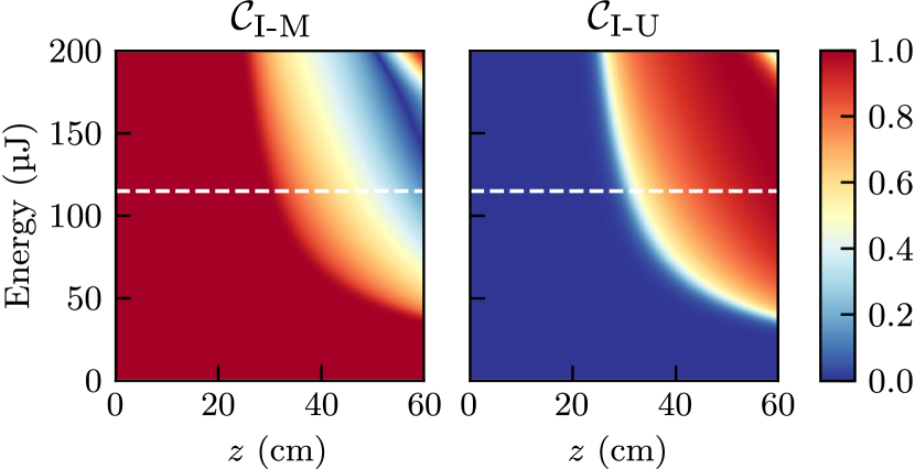
Figure 4: Concurrence as a function of the initial pump beam energy and the propagation distance $\bm{z}$. The plots show the evolution of the idler-mixing $\mathcal{C}_{\text{I-M}}$ and idler-up-converted $\mathcal{C}_{\text{I-U}}$ concurrences at a pressure of 70 bar. The white dashed lines correspond to the evolution displayed in Fig. 3.

In conclusion, we have explored the use of molecular modulation triggered by SRS in gas-filled ARFs for frequency up-conversion of entangled photon pairs, showing how entanglement can be efficiently transferred to the frequency-converted mode. To do so, we introduced a full quantum Hamiltonian description of the system capable of recovering the Maxwell-Bloch equations in the semiclassical limit. With it, we were able to characterize the state of the molecules as the vibrational coherence is established, and to use it in the analysis of the molecular modulation of quantum light states injected in H₂-filled ARFs. We derived simple expressions governing the evolution of entanglement in the system that predict a close correlation with the evolution of the photon numbers. As the experiments in this area are rapidly progressing, we believe that this framework will be a useful resource for the design of novel fiber-based quantum transduction strategies that could be fully integrated with existing fiber networks, thereby bringing the dream of the future quantum networks one step closer.

Supplemental Material

I Experimental parameters

In this section, we present a list of the parameters extracted from the experiment in Ref. SM_Tyumenev2022 , which we have used to obtain the results presented in this manuscript.

List of experimental parameters
Parameter name	Symbol	Value	Units
$\text{H}_{2}$ pressure	$P$	70	bar
Temperature	$T$	298	K
Pulse energy	$E_{\text{pulse}}$	$1.15\times 10^{-4}$	J
Pulse temporal width	$T_{\text{width}}$	$8.5432\times 10^{-9}$	s
Number of molecules	$N$	$1.4925\times 10^{18}$	-
Raman shift	$\Omega/2\pi$	$1.2457\times 10^{14}$	Hz
Phase relaxation time	$T_{2}$	$9.6897\times 10^{-11}$	s
Damping rate	$\Gamma$	$1.0320\times 10^{10}$	Hz
fiber diameter	$D$	$1.1\times 10^{-4}$	m
fiber length	$L$	0.6	m
Effective area of the $\text{LP}_{01}$ mode	$A_{01}$	$1.4621\times 10^{-9}$	$\text{m}^{2}$
Total area of the fiber	$A_{\text{fiber}}$	$9.5033\times 10^{-9}$	$\text{m}^{2}$
Effective volume of the fiber	$\mathcal{V}_{\text{fiber}}$	$8.7723\times 10^{-10}$	$\text{m}^{3}$
Quantization volume	$\mathcal{V}$	$2.4340\times 10^{-8}$	$\text{m}^{3}$
Pump wavelength	$\lambda_{P}$	$1.064\times 10^{-6}$	m
Stokes wavelength	$\lambda_{S}$	$1.9072\times 10^{-6}$	m
Anti-Stokes wavelength	$\lambda_{A}$	$7.3781\times 10^{-7}$	m
Mixing wavelength	$\lambda_{M}$	$1.425\times 10^{-6}$	m
Up-converted wavelength	$\lambda_{U}$	$8.9503\times 10^{-7}$	m
Pump frequency	$\nu_{P}$	$2.8176\times 10^{14}$	Hz
Stokes frequency	$\nu_{S}$	$1.5719\times 10^{14}$	Hz
Anti-Stokes frequency	$\nu_{A}$	$4.0633\times 10^{14}$	Hz
Mixing frequency	$\nu_{M}$	$2.1038\times 10^{14}$	Hz
Up-converted frequency	$\nu_{U}$	$3.3495\times 10^{14}$	Hz
Gain pump-Stokes	$\gamma_{p-s}$	$9.7644\times 10^{-12}$	$\text{m W}^{-1}$
Gain mixing-up-converted	$\gamma_{m-u}$	$1.3233\times 10^{-11}$	$\text{m W}^{-1}$
Coupling pump-Stokes	$\kappa_{1,p}$	$-8.9518\times 10^{-8}$	$\text{m}^{2}\text{ C}^{2}\text{ J}^{-2}\text{ s}^{-1}$
Coupling mixing-up-converted	$\kappa_{1,u}$	$-9.0080\times 10^{-8}$	$\text{m}^{2}\text{ C}^{2}\text{ J}^{-2}\text{ s}^{-1}$

Table 1: Table containing experimental parameters from Ref. SM_Tyumenev2022 used in the simulations displayed in this letter.

The number of molecules is computed using the ideal gas law,

$$N=\frac{P\mathcal{V}_{\text{fiber}}}{k_{\text{B}}T},$$ (S1)

where $k_{\text{B}}=1.380649\times 10^{-23}\text{ J K}^{-1}$ is the Boltzmann constant, $T$ is the temperature in Kelvin, $\mathcal{V}_{\text{fiber}}$ is the volume of the fiber in $\text{m}^{3}$, and $P$ is the pressure in Pa. Meanwhile, the total number of photons is calculated by dividing the energy of the pulse by the energy of a single pump photon, yielding $N_{\text{photons}}=6.1598\times 10^{14}$. The interaction strengths used in this letter are computed in terms of the couplings given in Table 1, as

$$G_{S} = -\kappa_{1,p}\frac{h\sqrt{\nu_{P}\nu_{S}}}{2\epsilon_{0}\mathcal{V}}=2.8962\times 10^{-8}\text{ Hz},$$ (S2)

$$G_{U} = -\kappa_{1,u}\frac{h\sqrt{\nu_{U}\nu_{M}}}{2\epsilon_{0}\mathcal{V}}=3.6760\times 10^{-8}\text{ Hz}.$$ (S3)

Here, $\epsilon_{0}$ is the electric permittivity of the vacuum, and $\mathcal{V}$ is the quantization volume of the fields. The couplings are computed using the phenomenological relations Bauerschmidt2016

$$\kappa_{1,p} = -\sqrt{\frac{2\gamma_{p-s}c^{2}\Gamma\epsilon_{0}^{2}}{N_{\rho}\hbar(\omega_{P}-\Omega)}},$$ (S4)

$$\kappa_{1,u} = -\sqrt{\frac{2\gamma_{m-u}c^{2}\Gamma\epsilon_{0}^{2}}{N_{\rho}\hbar(\omega_{U}-\Omega)}}.$$ (S5)

On the other hand, $\mathcal{V}$ is obtained by multiplying the total area of the fiber $A_{\text{fiber}}$ by the temporal width of the pulse $T_{\text{width}}$ and the speed of light $c$, i.e., $\mathcal{V}=cT_{\text{width}}A_{\text{fiber}}$. In this sense, $\mathcal{V}$ would follow the textbook definition of relevant volume that contains the energy of the radiation field, taking the volume integral of the electromagnetic energy density as reference. In order to provide a reasonable analytical expression for this volume, knowing that the real pulse has a finite duration, we define the temporal profile of the pulse as a piecewise function that is zero everywhere except in the relevant pulse region, where it would follow an amplitude distribution. In this regard, we consider the Bessel function $J_{0}$. Therefore, $T_{\text{width}}$ is estimated through the distance between the first zeros of $J_{0}$ that approximates the Gaussian distribution considered in Ref. SM_Tyumenev2022 for the pulse profile. The Bessel function used is determined by matching the integral of its square to the integral of the square of the previously mentioned Gaussian distribution in order to obtain the same total pulse energy while maintaining the same field amplitude factor. For the pulse transversal profile area, following the definition of volume containing the radiation, we considered $A_{\text{fiber}}$. This area is given by the inner diameter of the fiber at Ref. SM_Tyumenev2022 , excluding the capillaries. This is considered because, although hollow-core anti-resonant fibers present extremely low losses and provide tight modal confinement in the hollow region at the center of the multi-capillary microstructure, there is still some residual light intensity outside of the pulse's effective mode area. With this approach, the value obtained for $\mathcal{V}$ leads to reasonable dynamics given the evolution time, given that $G_{S}$ and $G_{U}$ depend on the quantization volume.

In Fig. S1, we present the evolution of $\alpha_{P}$ and $\alpha_{S}$, the amplitudes of the coherent states that characterize the pump and the Stokes pulses inside the fiber, as studied in Ref. SM_Tyumenev2022 . In this study, molecular coherence inside a hollow-core fiber filled with hydrogen gas is developed through a stimulated Raman scattering process. A pump tone is used to excite the molecules, producing an increase on the population of the corresponding Stokes mode, as one can see in Fig. S1. In green, one can see the normalized amplitude of the pump field while, in red, we have the normalized amplitude of Stokes photons. Most of all dynamics occur at the latter half of the fiber, where coherence starts to develop.

Figure S1: Evolution of the normalized amplitudes of the coherent states describing the pump and Stokes pulses during stimulated Raman scattering inside a hollow-core fiber filled with hydrogen gas as a function of the fiber length. We represent the normalized $\alpha_{P}$ and $\alpha_{S}$ in green and in red, respectively, against the length of the fiber. This figure illustrates how a coherent state is developed in the Stokes mode through the fiber, which leads to a depletion of the pump. Meanwhile, coherence is being developed in the molecules, gaining relevance at around the half-length of the fiber, when the pump and Stokes amplitudes start to change.

II From original to effective Hamiltonian

The Hamiltonian describing the process of Raman scattering can be split into an unperturbed part, $H_{0}$, and an interaction part, $V$. On the one hand, the unperturbed Hamiltonian can be expressed as

$$H_{0}=\hbar\omega_{0}|0\rangle\langle 0|+\hbar\omega_{1}|1\rangle\langle 1|+\hbar\sum_{i=2}^{\infty}\omega_{i}|i\rangle\langle i|+\hbar\sum_{l}\omega_{l}a^{\dagger}_{l}a_{l},$$ (S6)

where $\omega_{i}$ is the frequency associated to the transition between vibrational levels $|i\rangle$ and $|i+1\rangle$ of the molecule, whereas $\omega_{l}$ represents the frequency of mode $l$ of the electric field, with $l\in\{P,S,A\}$ labelling the pump, Stokes, and anti-Stokes modes, respectively. On the other hand, we derive the interaction Hamiltonian, assuming that the interaction is dipolar, from the term $-\vec{\bf\mu}\vec{\bf E}(z)$. Here, $\vec{\bf\mu}$ and $\vec{\bf E}(z)$ are the dipole and the electric field operators, respectively, and can be written as

$$\vec{\bf\mu} = \vec{e}\sum_{i,j}\mu_{i,j}|i\rangle\langle j|,$$ (S7)

$$\vec{\bf E}(z) = i\vec{f}\sqrt{\frac{\hbar\omega}{2\epsilon_{0}\mathcal{V}}}\left(ae^{i\beta z}-a^{\dagger}e^{-i\beta z}\right).$$ (S8)

If these two are aligned, $\vec{e}\vec{f}=1$, we can write the interaction term as

$$-\vec{\bf\mu}\,\vec{\bf E}(z)=\sum_{i,j}g_{i,j}|i\rangle\langle j|\left(ae^{i\beta z}-a^{\dagger}e^{-i\beta z}\right),$$ (S9)

where we have defined

$$g_{i,j}=-i\mu_{i,j}\sqrt{\frac{\hbar\omega}{2\epsilon_{0}\mathcal{V}}}.$$ (S10)

Notice that $g_{j,i}=-g_{i,j}^{*}$ has units of energy. Then, the interaction term for the Hamiltonian is given by

$$V=\sum_{i,j}\sum_{l}g_{i,j}^{l}|i\rangle\langle j|\left(a_{l}e^{i\beta_{l}z}-a_{l}^{\dagger}e^{-i\beta_{l}z}\right).$$ (S11)

Now, we want to make an interaction picture transformation and eliminate the energy levels with $i>1$ from the Hamiltonian. We assume these levels are off resonance, and focus on the resonant transition between the ground state $|0\rangle$ and the first vibrational state $|1\rangle$. First, we go to an interaction picture with respect to $H_{0}$. For that, let us propose a splitting of the evolution operator into $U=U_{0}U_{t}$, such that the Schrödinger equation reads

$$i\hbar\partial_{t}(U_{0}U_{t})=(H_{0}+V)U_{0}U_{t}.$$ (S12)

If we expand the derivative, we arrive at

$$i\hbar U_{0}(\partial_{t}U_{t})+(i\hbar\partial_{t}U_{0}-H_{0}U_{0})U_{t}=VU_{0}U_{t}.$$ (S13)

We have that $i\partial_{t}U_{0}-H_{0}U_{0}=0$, since it is the Schrödinger equation for $H_{0}$, and we are left with

$$i\hbar\partial_{t}U_{t}=U_{0}^{\dagger}VU_{0}U_{t}.$$ (S14)

Assuming that $U_{0}=e^{-iH_{0}t/\hbar}$, because $H_{0}$ is not time dependent, the solution for $U_{t}$ is

$$U_{t} = \hat{T}e^{-\frac{i}{\hbar}\int_{0}^{t}\text{d}s\,e^{iH_{0}s/\hbar}Ve^{-iH_{0}s/\hbar}}=\text{1}-\frac{i}{\hbar}\int_{0}^{t}\text{d}s\,e^{iH_{0}s/\hbar}Ve^{-iH_{0}s/\hbar}$$ (S15)

$$+ \frac{(-i)^{2}}{\hbar^{2}}\int_{0}^{t}\text{d}s\,e^{iH_{0}s/\hbar}Ve^{-iH_{0}s/\hbar}\int_{0}^{s}\text{d}s^{\prime}\,e^{iH_{0}s^{\prime}/\hbar}Ve^{-iH_{0}s^{\prime}/\hbar}+\ldots,$$

what is know as the Dyson series, with $\hat{T}$ being the time-ordering operator. Knowing the following formula,

$$e^{A}Be^{-A}=\sum_{k=0}^{\infty}\frac{1}{k!}[A,[A,\ldots,[A,B]\ldots]]_{k},$$ (S16)

we compute the commutators of $H_{0}$ with $V$,

$$[H_{0},V] = \hbar\sum_{i,j}\sum_{l}g_{i,j}^{l}|i\rangle\langle j|\left[(\omega_{i}-\omega_{j}-\nu_{l})a_{l}e^{i\beta_{l}z}-(\omega_{i}-\omega_{j}+\nu_{l})a^{\dagger}_{l}e^{-i\beta_{l}z}\right],$$ (S17)

$$[H_{0},[H_{0},V]] = \hbar^{2}\sum_{i,j}\sum_{l}g_{i,j}^{l}|i\rangle\langle j|\left[(\omega_{i}-\omega_{j}-\nu_{l})^{2}a_{l}e^{i\beta_{l}z}-(\omega_{i}-\omega_{j}+\nu_{l})^{2}a^{\dagger}_{l}e^{-i\beta_{l}z}\right].$$

We can infer from this that

$$e^{iH_{0}t/\hbar}Ve^{-iH_{0}t/\hbar}\equiv V_{I}(t)=\sum_{i,j}\sum_{l}g_{i,j}^{l}|i\rangle\langle j|e^{i(\omega_{i}-\omega_{j})t}\left(a_{l}e^{i(\beta_{l}z-\omega_{l}t)}-a_{l}^{\dagger}e^{-i(\beta_{l}z-\omega_{l}t)}\right).$$ (S18)

As it is often done in time-dependent perturbation theory, we expand to second order in $U_{t}$,

$$U_{t}=\text{1}-\frac{i}{\hbar}\int_{0}^{t}\text{d}s\,e^{iH_{0}s/\hbar}Ve^{-iH_{0}s/\hbar}-\frac{1}{\hbar^{2}}\int_{0}^{t}\text{d}s\,e^{iH_{0}s/\hbar}Ve^{-iH_{0}s/\hbar}\int_{0}^{s}\text{d}s^{\prime}\,e^{iH_{0}s^{\prime}/\hbar}Ve^{-iH_{0}s^{\prime}/\hbar},$$ (S19)

and compare it to the propagator given by the effective Hamiltonian we want to find,

$$U_{\text{eff}}(t)=\text{1}-\frac{i}{\hbar}\int_{0}^{t}\text{d}s\,H_{\text{eff}}(s)+\ldots,$$ (S20)

which is normally kept at first order. We assume that the first-order term in $U_{t}$ can be adiabatically eliminated because $g_{i,j}^{l}\ll\omega_{i}-\omega_{j}\pm\omega_{l}$. Therefore, we are set to compare the terms $V_{I}(s)V_{I}(s^{\prime})$ and $H_{\text{eff}}(s)$. We expand the latter and write

$$V_{I}(s)V_{I}(s^{\prime}) = \sum_{i,j,k}\sum_{l,m}g_{i,j}^{l}g_{j,k}^{m}|i\rangle\langle k|\Big{(}a^{\dagger}_{l}a^{\dagger}_{m}e^{-i(\beta_{l}+\beta_{m})z}e^{i(\omega_{i}-\omega_{j}+\omega_{l})s}e^{i(\omega_{j}-\omega_{k}+\omega_{m})s}$$

$$- a^{\dagger}_{l}a_{m}e^{-i(\beta_{l}-\beta_{m})z}e^{i(\omega_{i}-\omega_{j}+\omega_{l})s}e^{i(\omega_{j}-\omega_{k}-\omega_{m})s}-a_{l}a^{\dagger}_{m}e^{i(\beta_{l}-\beta_{m})z}e^{i(\omega_{i}-\omega_{j}-\omega_{l})s}e^{i(\omega_{j}-\omega_{k}+\omega_{m})s}$$

$$+ a_{l}a_{m}e^{i(\beta_{l}+\beta_{m})z}e^{i(\omega_{i}-\omega_{j}-\omega_{l})s}e^{i(\omega_{j}-\omega_{k}-\omega_{m})s}\Big{)}.$$

Since we want to identify $-iH_{\text{eff}}(s)/\hbar$ with $-V_{I}(s)\int_{0}^{s}\text{d}s^{\prime}\,V_{I}(s^{\prime})/\hbar^{2}$, we need to perform the integral over $s^{\prime}$:

$$V_{I}(s)\int_{0}^{s}\text{d}s^{\prime}\,V_{I}(s^{\prime})=-i\sum_{i,j,k}\sum_{l,m}g_{i,j}^{l}g_{j,k}^{m}|i\rangle\langle k|\Big{[}\frac{a^{\dagger}_{l}a^{\dagger}_{m}e^{-i(\beta_{l}+\beta_{m})z}}{\omega_{j}-\omega_{k}+\omega_{m}}\Big{(}e^{i(\omega_{i}-\omega_{k}+\omega_{l}+\omega_{m})s}-e^{i(\omega_{i}-\omega_{j}+\omega_{l})s}\Big{)}$$

$$-\frac{a^{\dagger}_{l}a_{m}e^{-i(\beta_{l}-\beta_{m})z}}{\omega_{j}-\omega_{k}-\omega_{m}}\Big{(}e^{i(\omega_{i}-\omega_{k}+\omega_{l}-\omega_{m})s}-e^{i(\omega_{i}-\omega_{j}+\omega_{l})s}\Big{)}-\frac{a_{l}a^{\dagger}_{m}e^{i(\beta_{l}-\beta_{m})z}}{\omega_{j}-\omega_{k}+\omega_{m}}\Big{(}e^{i(\omega_{i}-\omega_{k}-\omega_{l}+\omega_{m})s}-e^{i(\omega_{i}-\omega_{j}-\omega_{l})s}\Big{)}$$

$$+\frac{a_{l}a_{m}e^{i(\beta_{l}+\beta_{m})z}}{\omega_{j}-\omega_{k}-\omega_{m}}\Big{(}e^{i(\omega_{i}-\omega_{k}-\omega_{l}-\omega_{m})s}-e^{i(\omega_{i}-\omega_{j}-\omega_{l})s}\Big{)}\Big{]}.$$ (S21)

Basically, we are now going to neglect all rotating terms, in the approximation mentioned before. For this, we need to identify the resonant frequencies in the system. We define $\Omega_{i,j}\equiv\omega_{i}-\omega_{j}$, and identify $\Omega_{1,0}\equiv\Omega$ as the molecules vibrational transition frequency. Then, we can identify two resonances in the system, a Stokes and an anti-Stokes one, defined in relation to the pump frequency,

$$\Omega=\omega_{P}-\omega_{S}=\omega_{A}-\omega_{P}.$$ (S22)

Let us now compute the elements of $V_{I}(s)\int_{0}^{s}\text{d}s^{\prime}\,V_{I}(s^{\prime})$ in the basis of $\{|0\rangle,|1\rangle\}$,

$$\langle 0|V_{I}(s)\int_{0}^{s}\text{d}s^{\prime}\,V_{I}(s^{\prime})|0\rangle=i\sum_{k}|g_{0,k}^{l}|^{2}\sum_{l}\left(\frac{a_{l}^{\dagger}a_{l}}{\Omega_{k,0}-\omega_{l}}+\frac{a_{l}a_{l}^{\dagger}}{\Omega_{k,0}+\omega_{l}}\right),$$

$$\langle 0|V_{I}(s)\int_{0}^{s}\text{d}s^{\prime}\,V_{I}(s^{\prime})|1\rangle=i\sum_{k}\left[a^{\dagger}_{P}a_{S}e^{-i\Delta\beta z}\left(\frac{g_{0,k}^{P}g_{k,1}^{S}}{\Omega_{k,1}-\omega_{S}}+\frac{g_{0,k}^{S}g_{k,1}^{P}}{\Omega_{k,1}+\omega_{P}}\right)+a^{\dagger}_{A}a_{P}e^{-i\Delta\beta^{\prime}z}\left(\frac{g_{0,k}^{A}g_{k,1}^{P}}{\Omega_{k,1}-\omega_{P}}+\frac{g_{0,k}^{P}g_{k,1}^{A}}{\Omega_{k,1}+\omega_{A}}\right)\right],$$

$$\langle 1|V_{I}(s)\int_{0}^{s}\text{d}s^{\prime}\,V_{I}(s^{\prime})|0\rangle=i\sum_{k}\left[a_{P}a^{\dagger}_{S}e^{i\Delta\beta z}\left(\frac{g_{1,k}^{S}g_{k,0}^{P}}{\Omega_{k,0}-\omega_{P}}+\frac{g_{1,k}^{P}g_{k,0}^{S}}{\Omega_{k,0}+\omega_{S}}\right)+a_{A}a^{\dagger}_{P}e^{i\Delta\beta^{\prime}z}\left(\frac{g_{1,k}^{P}g_{k,0}^{A}}{\Omega_{k,0}-\omega_{A}}+\frac{g_{1,k}^{A}g_{k,0}^{P}}{\Omega_{k,0}+\omega_{P}}\right)\right],$$

$$\langle 1|V_{I}(s)\int_{0}^{s}\text{d}s^{\prime}\,V_{I}(s^{\prime})|1\rangle=i\sum_{k}|g_{1,k}^{l}|^{2}\sum_{l}a^{\dagger}_{l}a_{l}\left(\frac{1}{\Omega_{k,1}-\omega_{l}}+\frac{1}{\Omega_{k,1}+\omega_{l}}\right).$$

See that we have identified $\Delta\beta\equiv\beta_{P}-\beta_{S}$ and $\Delta\beta^{\prime}\equiv\beta_{A}-\beta_{P}$. Then, we identify $H_{\text{eff}}$ as $-iV_{I}(s)\int_{0}^{s}\text{d}s^{\prime}\,V_{I}(s^{\prime})/\hbar$, and write

$$H_{\text{eff}}^{I}(t) = \hbar\sum_{l}a^{\dagger}_{l}a_{l}\left(\delta_{0,l}|0\rangle\langle 0|+\delta_{1,l}|1\rangle\langle 1|\right)+\hbar\left(G_{0,1}^{S}a^{\dagger}_{P}a_{S}e^{-i\Delta\beta z}e^{-i(\Omega-\omega_{P}+\omega_{S})t}+G_{0,1}^{A}a_{P}a^{\dagger}_{A}e^{-i\Delta\beta^{\prime}z}e^{-i(\Omega-\omega_{A}+\omega_{P})t}\right)|0\rangle\langle 1|$$ (S23)

$$+ \left(G_{1,0}^{S}a_{P}a^{\dagger}_{S}e^{i\Delta\beta z}e^{i(\Omega-\omega_{P}+\omega_{S})t}+G_{1,0}^{A}a^{\dagger}_{P}a_{A}e^{i\Delta\beta^{\prime}z}e^{i(\Omega-\omega_{A}+\omega_{P})t}\right)|1\rangle\langle 0|.$$

Notice that this is defined in the interaction picture. In this Hamiltonian, we defined the following coefficients

$$\delta_{0,l} = -\frac{1}{\hbar^{2}}\sum_{k}|g_{0,k}^{l}|^{2}\left(\frac{1}{\Omega_{k,0}-\omega_{l}}+\frac{1}{\Omega_{k,0}+\omega_{l}}\right),$$ (S24)

$$\delta_{1,l} = -\frac{1}{\hbar^{2}}\sum_{k}|g_{1,k}^{l}|^{2}\left(\frac{1}{\Omega_{k,1}-\omega_{l}}+\frac{1}{\Omega_{k,1}+\omega_{l}}\right).$$ (S25)

These are often referred to as dynamic Stark shifts. Furthermore, we have also defined

$$G_{0,1}^{S}=\frac{1}{\hbar^{2}}\sum_{k}\left(\frac{g_{0,k}^{P}g_{k,1}^{S}}{\Omega_{k,1}-\omega_{S}}+\frac{g_{0,k}^{S}g_{k,1}^{P}}{\Omega_{k,1}+\omega_{P}}\right),$$ (S26)

$$G_{0,1}^{A}=\frac{1}{\hbar^{2}}\sum_{k}\left(\frac{g_{0,k}^{A}g_{k,1}^{P}}{\Omega_{k,1}-\omega_{P}}+\frac{g_{0,k}^{P}g_{k,1}^{A}}{\Omega_{k,1}+\omega_{A}}\right),$$ (S27)

$$G_{1,0}^{S}=\frac{1}{\hbar^{2}}\sum_{k}\left(\frac{g_{1,k}^{S}g_{k,0}^{P}}{\Omega_{k,0}-\omega_{P}}+\frac{g_{1,k}^{P}g_{k,0}^{S}}{\Omega_{k,0}+\omega_{S}}\right),$$ (S28)

$$G_{1,0}^{A}=\frac{1}{\hbar^{2}}\sum_{k}\left(\frac{g_{1,k}^{P}g_{k,0}^{A}}{\Omega_{k,0}-\omega_{A}}+\frac{g_{1,k}^{A}g_{k,0}^{P}}{\Omega_{k,0}+\omega_{P}}\right).$$ (S29)

Notice that here we can identify $G_{1,0}^{S}\equiv G_{S}$ and $G_{1,0}^{A}\equiv G_{A}$, such that $G_{0,1}^{S}=G_{S}^{*}$ and $G_{0,1}^{A}=G_{A}^{*}$, assuming that $g_{j,i}=g_{i,j}^{*}$. Then, we can write

$$G_{S}=\frac{1}{\hbar^{2}}\sum_{k}\left(\frac{g_{1,k}^{S}g_{k,0}^{P}}{\Omega_{k,0}-\omega_{P}}+\frac{g_{1,k}^{P}g_{k,0}^{S}}{\Omega_{k,0}+\omega_{S}}\right),$$ (S30)

$$G_{A}=\frac{1}{\hbar^{2}}\sum_{k}\left(\frac{g_{1,k}^{P}g_{k,0}^{A}}{\Omega_{k,0}-\omega_{A}}+\frac{g_{1,k}^{A}g_{k,0}^{P}}{\Omega_{k,0}+\omega_{P}}\right).$$ (S31)

Let us point out some equivalences between frequencies,

$$\Omega_{k,1}-\omega_{S} = \Omega_{k,0}-\omega_{P},$$

$$\Omega_{k,1}+\omega_{P} = \Omega_{k,0}+\omega_{S},$$

$$\Omega_{k,1}-\omega_{P} = \Omega_{k,0}-\omega_{A},$$

$$\Omega_{k,1}+\omega_{A} = \Omega_{k,0}+\omega_{P}.$$

Let us now write the effective Hamiltonian in the Schrödinger picture. We just have to cancel the exponentials, and recover the original Hamiltonian, $H_{0}$.

$$H_{\text{eff}} = H_{0}+e^{-iH_{0}t/\hbar}H_{\text{eff}}^{I}(t)e^{iH_{0}t/\hbar}=\hbar\omega_{0}|0\rangle\langle 0|+\hbar\omega_{1}|1\rangle\langle 1|+\hbar\sum_{l}\omega_{l}a^{\dagger}_{l}a_{l}(|0\rangle\langle 0|+|1\rangle\langle 1|)+\hbar\sum_{l}a^{\dagger}_{l}a_{l}\left(\delta_{0,l}|0\rangle\langle 0|+\delta_{1,l}|1\rangle\langle 1|\right)$$ (S32)

$$+ \hbar\left(G_{S}e^{i\Delta\beta z}a_{P}a^{\dagger}_{S}+G_{A}e^{i\Delta\beta^{\prime}z}a^{\dagger}_{P}a_{A}\right)|1\rangle\langle 0|+\hbar\left(G_{S}^{*}e^{-i\Delta\beta z}a^{\dagger}_{P}a_{S}+G_{A}^{*}e^{-i\Delta\beta^{\prime}z}a_{P}a^{\dagger}_{A}\right)|0\rangle\langle 1|.$$

We can rewrite this by replacing $|1\rangle\langle 1|=(\text{1}+\sigma_{z})/2$, $|0\rangle\langle 0|=(\text{1}-\sigma_{z})/2$, $|1\rangle\langle 0|=\sigma^{+}$, and $|0\rangle\langle 1|=\sigma^{-}$. We will neglect the constant term $\text{1}(\omega_{0}+\omega_{1})/2$, and define $\Delta_{l}^{\pm}=(\delta_{1,l}\pm\delta_{0,l})/2$. Finally, we obtain

$$H_{\text{eff}} = \frac{\hbar\Omega}{2}\sigma_{z}+\hbar\sum_{l}\left(\omega_{l}+\Delta_{l}^{+}\right)a^{\dagger}_{l}a_{l}+\hbar\sum_{l}\Delta_{l}^{-}a^{\dagger}_{l}a_{l}\sigma_{z}+\hbar\left(G_{S}e^{i\Delta\beta z}a_{P}a^{\dagger}_{S}+G_{A}e^{i\Delta\beta^{\prime}z}a^{\dagger}_{P}a_{A}\right)\sigma^{+}$$

$$+ \hbar\left(G_{S}^{*}e^{-i\Delta\beta z}a^{\dagger}_{P}a_{S}+e^{-i\Delta\beta^{\prime}z}G_{A}^{*}a_{P}a^{\dagger}_{A}\right)\sigma^{-}.$$

In order to extend this to $N$ molecules, we need to replace $\sigma_{z}/2\rightarrow J_{z}$ and $\sigma^{\pm}\rightarrow J^{\pm}$, where we have identified

$$J_{z} = \frac{1}{2}\sum_{i=1}^{N}\mathbb{1}_{1}\otimes\ldots\otimes\mathbb{1}_{i-1}\otimes\sigma_{i}^{z}\otimes\mathbb{1}_{i+1}\otimes\ldots\otimes\mathbb{1}_{N},$$ (S34)

$$J^{\pm} = \sum_{i=1}^{N}\mathbb{1}_{1}\otimes\ldots\otimes\mathbb{1}_{i-1}\otimes\sigma_{i}^{\pm}\otimes\mathbb{1}_{i+1}\otimes\ldots\otimes\mathbb{1}_{N},$$ (S35)

with $[J_{z},J^{\pm}]=\pm J^{\pm}$, $[J^{+},J^{-}]=2J_{z}$, and the global spin states as $\left|{\bf\frac{N}{2}},m_{z}\right\rangle$, with $m_{z}\in\{-N/2,\ldots,N/2\}$. The global spin operators act on these states as follows,

$$J_{z}\left|{\bf\frac{N}{2}},m_{z}\right\rangle = m_{z}\left|{\bf\frac{N}{2}},m_{z}\right\rangle,$$ (S36)

$$J^{\pm}\left|{\bf\frac{N}{2}},m_{z}\right\rangle = \sqrt{\frac{N}{2}\left(\frac{N}{2}+1\right)-m_{z}\left(m_{z}\pm 1\right)}\left|{\bf\frac{N}{2}},m_{z}\right\rangle.$$ (S37)

With this, we can write the effective Hamiltonian describing the interaction with $N$ molecules,

$$H_{\text{eff}} = \hbar\Omega J_{z}+\hbar\sum_{l}\left(\omega_{l}+\Delta_{l}^{+}\right)a^{\dagger}_{l}a_{l}+2\hbar\sum_{l}\Delta_{l}^{-}a^{\dagger}_{l}a_{l}J_{z}+\hbar\left(G_{S}e^{i\Delta\beta z}a_{P}a^{\dagger}_{S}+G_{A}e^{i\Delta\beta^{\prime}z}a^{\dagger}_{P}a_{A}\right)J^{+}$$

$$+ \hbar\left(G_{S}^{*}e^{-i\Delta\beta z}a^{\dagger}_{P}a_{S}+e^{-i\Delta\beta^{\prime}z}G_{A}^{*}a_{P}a^{\dagger}_{A}\right)J^{-}.$$

III Equations of motion

Going back to the single-molecule case, we want to show that we can recover the Maxwell-Bloch equations describing stimulated Raman scattering through the equations of motion associated to the effective Hamiltonian we derived in the previous section. In the following, we only describe the pump-Stokes interaction, considering that the anti-Stokes population is negligible throughout the process. We will work with the Hamiltonian

$$H_{\text{eff}} = \frac{\hbar\Omega}{2}\sigma_{z}+\hbar\Big{[}(\omega_{P}+\Delta_{P}^{+})\mathbb{1}_{2}+\Delta_{P}^{-}\sigma_{z}\Big{]}a^{\dagger}_{P}a_{P}+\hbar\Big{[}(\omega_{S}+\Delta_{S}^{+})\mathbb{1}_{2}+\Delta_{S}^{-}\sigma_{z}\Big{]}a^{\dagger}_{S}a_{S}$$

$$+ \hbar\left(G_{S}e^{i\Delta\beta z}a_{P}a^{\dagger}_{S}\sigma^{+}+G_{S}^{*}e^{-i\Delta\beta z}a^{\dagger}_{P}a_{S}\sigma^{-}\right).$$

Here we will derive the equations of motion (EOM) that describe the change in populations in a single molecule due to the interaction with the pump and Stokes fields. First, we will start from the Stokes effective Hamiltonian, apply the semiclassical approximation on the pump and Stokes fields, and obtain the EOM. Note that these will include both a semiclassical and an adiabatic approximation. Another approach follows from the original Hamiltonian, applying a semiclassical approximation, and obtain the EOM, to finally apply the adiabatic approximation. The latter was the path taken in previous works, while the former is the path we want to follow. Our goal is to show that they are both equivalent.

We first start in the Schrödinger picture, and go to an interaction picture with respect to the pump and Stokes fields. We transform our Hamiltonian by $\omega_{P}a^{\dagger}_{P}a_{P}+\omega_{S}a^{\dagger}_{S}a_{S}$ obtaining the Hamiltonian

$$H_{\text{eff}}^{I}(t) = \frac{\hbar\Omega}{2}\sigma_{z}+\hbar\left(\Delta^{+}_{P}\mathbb{1}_{2}+\Delta_{P}^{-}\sigma_{z}\right)a^{\dagger}_{P}a_{P}+\hbar\left(\Delta^{+}_{S}\mathbb{1}_{2}+\Delta_{S}^{-}\sigma_{z}\right)a^{\dagger}_{S}a_{S}$$

$$+ \hbar\left(G_{S}e^{i\left(\Delta\beta z-\Omega t\right)}a_{P}a^{\dagger}_{S}\sigma^{+}+G_{S}^{*}e^{-i\left(\Delta\beta z-\Omega t\right)}a^{\dagger}_{P}a_{S}\sigma^{-}\right).$$

Now, we apply a semiclassical approximation in the bosonic modes, which amounts to replacing the associated creation and annihilation operators by their expectation values over a coherent state. That is, $a_{l}\rightarrow\alpha_{l}$ and $a_{l}^{\dagger}\rightarrow\alpha_{l}^{*}$ for $l\in\{P,S\}$,

$$H_{\alpha}^{I}(t) = \frac{\hbar\Omega}{2}\sigma_{z}+\hbar\left(\Delta^{+}_{P}\mathbb{1}_{2}+\Delta_{P}^{-}\sigma_{z}\right)|\alpha_{P}|^{2}+\hbar\left(\Delta^{+}_{S}\mathbb{1}_{2}+\Delta_{S}^{-}\sigma_{z}\right)|\alpha_{S}|^{2}$$

$$+ \hbar\left(G_{S}e^{i\left(\Delta\beta z-\Omega t\right)}\alpha_{P}\alpha_{S}^{*}\sigma^{+}+G_{S}^{*}e^{-i\left(\Delta\beta z-\Omega t\right)}\alpha_{P}^{*}\alpha_{S}\sigma^{-}\right).$$

The equations of motion for the state of the molecule, $\rho$, are computed using the von Neumann equation, $\hbar\dot{\rho}=i[\rho,H]$. We can split $\rho$ into its basis operators,

$$\rho=\rho_{0,0}\left(\frac{\mathbb{1}_{2}-\sigma_{z}}{2}\right)+\rho_{0,1}\sigma^{-}+\rho_{1,0}\sigma^{+}+\rho_{1,1}\left(\frac{\mathbb{1}_{2}+\sigma_{z}}{2}\right)=\mathbb{1}_{2}+(\rho_{1,1}-\rho_{0,0})\frac{\sigma_{z}}{2}+\rho_{0,1}\sigma^{-}+\rho_{1,0}\sigma^{+},$$ (S42)

since $\rho_{1,1}+\rho_{0,0}=\tr\rho=1$, and express $[\rho,H]$ in such basis. For that, we compute

$$[\sigma_{z},H] = 2\hbar\left(G_{S}e^{i\left(\Delta\beta z-\Omega t\right)}\alpha_{P}\alpha_{S}^{*}\sigma^{+}-G_{S}^{*}e^{-i\left(\Delta\beta z-\Omega t\right)}\alpha_{P}^{*}\alpha_{S}\sigma^{-}\right),$$

$$[\sigma^{+},H] = -\hbar\left(\Omega+2\Delta_{P}^{-}|\alpha_{P}|^{2}+2\Delta_{S}^{-}|\alpha_{S}|^{2}\right)\sigma^{+}+\hbar G_{S}^{*}e^{-i\left(\Delta\beta z-\Omega t\right)}\alpha_{P}^{*}\alpha_{S}\sigma_{z},$$

$$[\sigma^{-},H] = \hbar\left(\Omega+2\Delta_{P}^{-}|\alpha_{P}|^{2}+2\Delta_{S}^{-}|\alpha_{S}|^{2}\right)\sigma^{-}-\hbar G_{S}e^{i\left(\Delta\beta z-\Omega t\right)}\alpha_{P}\alpha_{S}^{*}\sigma_{z},$$

using the formulas

$$[\sigma_{z},\sigma^{+}] = 2\sigma^{+},$$

$$[\sigma_{z},\sigma^{-}] = -2\sigma^{-},$$

$$[\sigma^{+},\sigma^{-}] = \sigma_{z}.$$

By defining $w=\rho_{1,1}-\rho_{0,0}$, we write the following EOM,

$$\dot{w} = -2i\left(\rho_{0,1}(t)G_{S}e^{i\left(\Delta\beta z-\Omega t\right)}\alpha_{P}\alpha_{S}^{*}-\rho_{1,0}(t)G_{S}^{*}e^{-i\left(\Delta\beta z-\Omega t\right)}\alpha_{P}^{*}\alpha_{S}\right),$$ (S43)

$$\dot{\rho}_{0,1} = i\rho_{0,1}(t)\left(\Omega+2\Delta_{P}^{-}|\alpha_{P}|^{2}+2\Delta_{S}^{-}|\alpha_{S}|^{2}\right)-iw(t)G_{S}^{*}e^{-i\left(\Delta\beta z-\Omega t\right)}\alpha_{P}^{*}\alpha_{S},$$ (S44)

$$\dot{\rho}_{1,0} = -i\rho_{1,0}(t)\left(\Omega+2\Delta_{P}^{-}|\alpha_{P}|^{2}+2\Delta_{S}^{-}|\alpha_{S}|^{2}\right)+iw(t)G_{S}e^{i\left(\Delta\beta z-\Omega t\right)}\alpha_{P}\alpha_{S}^{*}.$$ (S45)

Generally, the $\Delta_{l}^{-}$ terms are Stark shifts that can be neglected SM_Raymer1990 . In order for this result to match the Maxwell-Bloch equations SM_Raymer1990 ; Bauerschmidt2016 , we need to identify $G_{S}\alpha_{P}\alpha_{S}^{*}=-\kappa_{1,p}E_{P}E_{S}^{*}$. Using this relation, we estimate $G_{S}$ in terms of the phenomenological factor $\kappa_{1,p}$. This leaves us with

$$\dot{w} = 2i\left(\rho_{0,1}(t)\kappa_{1,p}E_{P}E_{S}^{*}e^{i\left(\Delta\beta z-\Omega t\right)}-\rho_{1,0}(t)\kappa^{*}_{1,p}E_{P}^{*}E_{S}e^{-i\left(\Delta\beta z-\Omega t\right)}\right),$$ (S46)

$$\dot{\rho}_{0,1} = i\rho_{0,1}(t)\Omega+iw(t)\kappa_{1,p}^{*}E_{P}^{*}E_{S}e^{-i\left(\Delta\beta z-\Omega t\right)},$$ (S47)

where we have not written the equation for $\dot{\rho}_{10}$ because it is just the complex conjugate of that for $\dot{\rho}_{0,1}$. The differences we find with the previous results lie in the definition of the electric field. While we have defined $\mathcal{E}(z,t)=\mathcal{E}_{P}(z,t)+\mathcal{E}_{S}(z,t)$, previous works defined $\mathcal{E}(z,t)=(\mathcal{E}_{P}(z,t)+\mathcal{E}_{S}(z,t))/2$, and thus the extra factor of $1/4$. Furthermore, while we have chosen the plain wave solution of the electric fields as

$$\mathcal{E}_{l}(z,t)=E_{l}e^{i(\beta_{l}z-\omega_{l}t)}+E_{l}^{*}e^{-i(\beta_{l}z-\omega_{l}t)},$$ (S48)

previous works have chosen

$$\mathcal{E}_{l}(z,t)=E_{l}e^{-i(\beta_{l}z-\omega_{l}t)}+E_{l}^{*}e^{i(\beta_{l}z-\omega_{l}t)},$$ (S49)

and this is why we find $E_{P}^{*}E_{S}$ instead of $E_{P}E_{S}^{*}$.

IV Spin Coherent State

The pump-Stokes N-molecule effective Hamiltonian in the Schrödinger picture is

$$H_{\text{eff}}=\hbar\Omega J_{z}+\hbar\omega_{P}a_{P}^{\dagger}a_{P}+\hbar\omega_{S}a_{S}^{\dagger}a_{S}+\hbar\left(G_{S}e^{i\Delta\beta z}a_{P}a_{S}^{\dagger}J^{+}+G_{S}^{*}e^{-i\Delta\beta z}a_{P}^{\dagger}a_{S}J^{-}\right),$$ (S50)

where we have neglected the Stark shifts $\Delta_{l}^{\pm}$. We now transform $H_{\text{eff}}$ to an interaction picture with respect to $\Omega J_{z}+\omega_{P}a_{P}^{\dagger}a_{P}+\omega_{S}a_{S}^{\dagger}a_{S}$ in order to avoid oscillations with frequency $\Omega$ of our observables. There, we find

$$H_{\text{eff}}^{I}=\hbar\left(G_{S}e^{i[(\Omega-\omega_{P}+\omega_{S})t+\Delta\beta z]}a_{P}a_{S}^{\dagger}J^{+}+G_{S}^{*}e^{-i[(\Omega-\omega_{P}+\omega_{S})t+\Delta\beta z]}a_{P}^{\dagger}a_{S}J^{-}\right).$$ (S51)

Notice that, in resonance conditions, $\Omega-\omega_{P}+\omega_{S}=0$, and there is no explicit time dependence in the Hamiltonian. Finally, we perform a semiclassical approximation on the pump and Stokes modes, $a_{l}\rightarrow\alpha_{l}$, and obtain

$$H_{\alpha}^{I}=\hbar\left(G_{S}e^{i\Delta\beta z}\alpha_{P}\alpha_{S}^{*}J^{+}+G_{S}^{*}e^{-i\Delta\beta z}\alpha_{P}^{*}\alpha_{S}J^{-}\right).$$ (S52)

We will write the propagator associated with this Hamiltonian as

$$e^{-itH_{\alpha}^{I}/\hbar}=e^{-it\left(\gamma J^{+}+\gamma^{*}J^{-}\right)}$$ (S53)

by defining $\gamma=G_{S}\alpha_{P}\alpha_{S}^{*}e^{i\Delta\beta z}$. Recall that the commutation relations for the global spin operators are

$$\left[J_{z},J^{\pm}\right] = \pm J^{\pm},$$ (S54)

$$\left[J^{+},J^{-}\right] = 2J_{z}.$$ (S55)

We assume that, since these commutators define a Lie algebra, there must be a relation such that Truax1985

$$e^{-it\left(\gamma J^{+}+\gamma^{*}J^{-}\right)}=e^{s(t)J^{+}}e^{s_{0}(t)J_{z}}e^{s_{1}(t)J^{-}},$$ (S56)

with $s(0)=s_{0}(0)=s_{1}(0)=0$. By differentiating by $t$ on both sides, and then multiplying by the inverse of the right-hand side, we find

$$-i\left(\gamma J^{+}+\gamma^{*}J^{-}\right)=\dot{s}(t)J^{+}+\dot{s}_{0}(t)e^{s(t)J^{+}}J_{z}e^{-s(t)J^{+}}+\dot{s}_{1}(t)e^{s(t)J^{+}}e^{s_{0}(t)J_{z}}J^{-}e^{-s_{0}(t)J_{z}}e^{-s(t)J^{+}}.$$ (S57)

Using the relation in Eq. (S16), we arrive at

$$-i\left(\gamma J^{+}+\gamma^{*}J^{-}\right)=\dot{s}(t)J^{+}+\dot{s}_{0}(t)\left(J_{z}-s(t)J^{+}\right)+\dot{s}_{1}(t)e^{-s_{0}(t)}\left(J^{-}+2s(t)J_{z}-s^{2}(t)J^{+}\right),$$ (S58)

from where we find the set of differential equations

$$\dot{s}(t)-\dot{s}_{0}(t)s(t)-\dot{s}_{1}(t)e^{-s_{0}(t)}s^{2}(t)=-i\gamma,$$ (S59)

$$\dot{s}_{1}(t)e^{-s_{0}(t)}=-i\gamma^{*},$$ (S60)

$$\dot{s}_{0}(t)+2\dot{s}_{1}(t)e^{-s_{0}(t)}s(t)=0.$$ (S61)

Notice that we can combine these to find

$$\dot{s}_{1}(t)e^{-s_{0}(t)}=-i\gamma^{*},$$ (S62)

$$\dot{s}_{0}(t)=2i\gamma^{*}s(t).$$ (S63)

and then we can isolate the equation for $s$,

$$\dot{s}(t)-i\gamma^{*}s^{2}(t)=-i\gamma.$$ (S64)

Solving this equation, we find

$$s(t)=-i\sqrt{\frac{\gamma}{\gamma^{*}}}\tan|\gamma|t.$$ (S65)

Using this to solve the remaining equations, we obtain

$$s_{1}(t) = -i\sqrt{\frac{\gamma^{*}}{\gamma}}\tan|\gamma|t,$$ (S66)

$$s_{0}(t) = -2\log\left(\cos|\gamma|t\right).$$ (S67)

Assuming that $\alpha_{P}$, $\alpha_{S}$, and $G_{S}$ are real, we can simplify these as

$$s(t) = e^{i\left(\Delta\beta z-\frac{\pi}{2}\right)}\tan\left(G_{S}\alpha_{P}\alpha_{S}t\right),$$ (S68)

$$s_{1}(t) = e^{-i\left(\Delta\beta z+\frac{\pi}{2}\right)}\tan\left(G_{S}\alpha_{P}\alpha_{S}t\right),$$ (S69)

$$s_{0}(t) = -2\log\left[\cos\left(G_{S}\alpha_{P}\alpha_{S}t\right)\right].$$ (S70)

Let us use this result to split the propagator $e^{-iH_{\alpha}^{I}t/\hbar}$, and obtain the state of the molecules at time $t$, assuming that they are initially in a ground state. In the interaction picture, the ground state of the molecules becomes

$$e^{-i\Omega t\frac{N}{2}}\left|{\bf\frac{N}{2}},-\frac{N}{2}\right\rangle.$$ (S71)

Then, we have that

$$|\psi_{I}(t)\rangle=e^{-i\Omega t\frac{N}{2}}e^{-iH_{\alpha}^{I}t/\hbar}\left|{\bf\frac{N}{2}},-\frac{N}{2}\right\rangle=e^{-i\Omega t\frac{N}{2}}e^{s(t)J^{+}}e^{s_{0}(t)J_{z}}e^{s_{1}(t)J^{-}}\left|{\bf\frac{N}{2}},-\frac{N}{2}\right\rangle,$$ (S72)

such that $e^{s_{1}(t)J^{-}}\left|{\bf\frac{N}{2}},-\frac{N}{2}\right\rangle=\left|{\bf\frac{N}{2}},-\frac{N}{2}\right\rangle$ and $e^{s_{0}(t)J_{z}}\left|{\bf\frac{N}{2}},-\frac{N}{2}\right\rangle=e^{-s_{0}(t)\frac{N}{2}}\left|{\bf\frac{N}{2}},-\frac{N}{2}\right\rangle$. We then find that

$$|\psi_{I}(t)\rangle=e^{-i\Omega t\frac{N}{2}}e^{-s_{0}(t)\frac{N}{2}}e^{s(t)J^{+}}\left|{\bf\frac{N}{2}},-\frac{N}{2}\right\rangle=e^{-i\Omega t\frac{N}{2}}e^{-s_{0}(t)\frac{N}{2}}\sum_{n=0}^{N}\frac{s^{n}(t)}{n!}(J^{+})^{n}\left|{\bf\frac{N}{2}},-\frac{N}{2}\right\rangle.$$ (S73)

If we compute explicitly the action of $J^{+}$, we find that

$$(J^{+})^{n}\left|{\bf\frac{N}{2}},-\frac{N}{2}\right\rangle=\sqrt{\frac{N!n!}{(N-n)!}}\left|{\bf\frac{N}{2}},-\frac{N}{2}+n\right\rangle,$$ (S74)

and we can write the final state of the molecules as

$$|\psi_{I}(t)\rangle=e^{-i\Omega t\frac{N}{2}}e^{-s_{0}(t)\frac{N}{2}}\sum_{n=0}^{N}\begin{pmatrix}N\\ n\end{pmatrix}^{1/2}s^{n}(t)\left|{\bf\frac{N}{2}},-\frac{N}{2}+n\right\rangle.$$ (S75)

This state should be normalized, so let us check if

$$\langle\psi_{I}(t)|\psi_{I}(t)\rangle=e^{-Ns_{0}(t)}\left(1+|s(t)|^{2}\right)^{N}=1.$$ (S76)

After some math, we can see that $s_{0}$ and $s$ are related through

$$e^{-s_{0}(t)}=\cos^{2}(G_{S}\alpha_{P}\alpha_{S}t)=\frac{1}{1+|s(t)|^{2}}.$$ (S77)

Therefore, we could write our state at time $t$ as

$$|\psi_{I}(t)\rangle=\left(\frac{e^{-i\Omega t}}{1+|s(t)|^{2}}\right)^{\frac{N}{2}}\sum_{n=0}^{N}\begin{pmatrix}N\\ n\end{pmatrix}^{1/2}s^{n}(t)\left|{\bf\frac{N}{2}},-\frac{N}{2}+n\right\rangle.$$ (S78)

Note that this state is expressed in the interaction picture of $\Omega J_{z}+\omega_{P}a_{P}^{\dagger}a_{P}+\omega_{S}a_{S}^{\dagger}a_{S}$; if we return to the Schrödinger picture, we find

$$|\psi(t)\rangle=\left(1+|s(t)|^{2}\right)^{-\frac{N}{2}}\sum_{n=0}^{N}\begin{pmatrix}N\\ n\end{pmatrix}^{1/2}\left(s(t)e^{-i\Omega t}\right)^{n}\left|{\bf\frac{N}{2}},-\frac{N}{2}+n\right\rangle.$$ (S79)

V Concurrence

After coherence has been generated in the molecule ensemble, we will send one mode of an entangled state through the fiber to change its frequency. Unlike coherence modulation, this is a thresholdless process which can be applied to single photons. We consider $(|0,0,0\rangle+|1,1,0\rangle)/\sqrt{2}$ as the initial state, where the states in tensor product, from left to right, indicate the idler mode, kept outside of the fiber, the mixing mode, which goes initially through the fiber, and the frequency-converted mode, initially in a vacuum state. While the phase-difference between the original and the frequency-converted signals has to be equal to the phase of the molecular coherence wave, the jump in frequency is given by the Raman shift. Therefore, even though this is not a Raman process, we can use the same interaction Hamiltonian to describe it. Furthermore, we will focus on the interaction between the pump and the anti-Stokes, since we are looking at frequency up-conversion. Then, we start from the Hamiltonian

$$H_{\text{eff}}=\hbar\Omega J_{z}+\hbar\omega_{M}a_{M}^{\dagger}a_{M}+\hbar\omega_{U}a_{U}^{\dagger}a_{U}+\hbar G_{U}\left(e^{-i(\beta_{M}-\beta_{U})z}a_{M}^{\dagger}a_{U}J^{+}+e^{i(\beta_{M}-\beta_{U})z}a_{M}a_{U}^{\dagger}J^{-}\right),$$ (S80)

where we have introduced $G_{U}$ as the coupling strength between the mixing, the up-converted and the molecules, which can be defined as

$$G_{U}=\frac{1}{\hbar^{2}}\sum_{k}\left(\frac{g_{1,k}^{M}g_{k,0}^{U}}{\Omega_{k,0}-\omega_{U}}+\frac{g_{1,k}^{U}g_{k,0}^{M}}{\Omega_{k,0}+\omega_{M}}\right).$$ (S81)

Again, we will go to an interaction picture, this time with respect to $\Omega J_{z}+\omega_{M}a_{M}^{\dagger}a_{M}+\omega_{U}a_{U}^{\dagger}a_{U}$, resulting in

$$H_{\text{eff}}^{I}=\hbar G_{U}\left(e^{i\big{[}(\Omega+\omega_{M}-\omega_{U})t-(\beta_{M}-\beta_{U})z\big{]}}a_{M}^{\dagger}a_{U}J^{+}+e^{-i\big{[}(\Omega+\omega_{M}-\omega_{U})t-(\beta_{M}-\beta_{U})z\big{]}}a_{M}a_{U}^{\dagger}J^{-}\right).$$ (S82)

Meanwhile, the molecules will be in a coherent state and, analogous to what we previously did for the bosonic modes, we will perform a semiclassical approximation. This time, we will assume the state of the molecules will not change when we introduce a single excitation into the fiber, and replace the global spin operators by their expectation values over the spin coherent state derived in the previous section. This way, we can define the variable

$$\xi=\langle s|J^{-}|s\rangle=\frac{Ns}{1+|s|^{2}}=\frac{N}{2}e^{i\left(\Delta\beta z-\frac{\pi}{2}\right)}\sin\left(2G_{S}\alpha_{P}\alpha_{S}t\right),$$ (S83)

in the interaction picture. This enters into our Hamiltonian as follows,

$$H^{I}_{\xi}=\hbar G_{U}\left(\xi^{*}e^{i\big{[}(\Omega+\omega_{M}-\omega_{U})t-(\beta_{M}-\beta_{U})z\big{]}}a_{M}^{\dagger}a_{U}+\xi e^{-i\big{[}(\Omega+\omega_{M}-\omega_{U})t-(\beta_{M}-\beta_{U})z\big{]}}a_{M}a_{U}^{\dagger}\right).$$ (S84)

Under phase matching and resonance conditions, we have $\beta_{U}-\beta_{M}=\Delta\beta$ and $\omega_{U}-\omega_{M}=\Omega$, respectively. Assuming these are satisfied, this Hamiltonian simplifies to

$$H^{I}_{\xi}=\hbar G_{U}\left(\xi^{*}e^{i\Delta\beta z}a_{M}^{\dagger}a_{U}+\xi e^{-i\Delta\beta z}a_{M}a_{U}^{\dagger}\right).$$ (S85)

As we can see, this resembles a beamsplitter operator. Now, we need to obtain the action of this Hamiltonian onto the initial state of the system, which will be $(|0,0,0\rangle+|1,1,0\rangle)/\sqrt{2}$. But first, we need to transform this state into the interaction picture,

$$\frac{1}{\sqrt{2}}\left(|0,0,0\rangle+e^{i\omega_{M}t}|1,1,0\rangle\right).$$ (S86)

We can easily see that $H_{\xi}^{I}|0,0,0\rangle=0$, as well as

$$H_{\xi}^{I}|1,1,0\rangle = \hbar G_{U}\xi e^{-i\Delta\beta z}|1,0,1\rangle,$$

$$H_{\xi}^{I}|1,0,1\rangle = \hbar G_{U}\xi^{*}e^{i\Delta\beta z}|1,1,0\rangle.$$

Since this forms a closed subspace for a single excitation, we can diagonalize the Hamiltonian in this subspace, finding that the energies are $E_{\xi}^{\pm}=\pm\hbar G_{U}|\xi|$. Therefore, we propose the eigenstates to be of the form $|\phi_{\xi}^{\pm}\rangle=a|1,1,0\rangle\pm b|1,0,1\rangle$. If we insert this into the eigenvalue equation, we find that the eigenstates are

$$|\phi_{\xi}^{\pm}\rangle=\frac{1}{\sqrt{2}}\left(|1,1,0\rangle\pm e^{-i\Delta\beta z}\sqrt{\frac{\xi}{\xi^{*}}}|1,0,1\rangle\right).$$ (S87)

With this, we can find the evolution of the initial state,

$$\frac{1}{\sqrt{2}}\left(|0,0,0\rangle+e^{i\omega_{M}t}\cos(G_{U}|\xi|t)|1,1,0\rangle-ie^{i(\omega_{M}t-\Delta\beta z)}\sqrt{\frac{\xi}{\xi^{*}}}\sin(G_{U}|\xi|t)|1,0,1\rangle\right).$$ (S88)

We can further simplify this by noticing that $\xi/\xi^{*}=e^{2i\left(\Delta\beta z-\frac{\pi}{2}\right)}$, such that the final state becomes

$$\frac{1}{\sqrt{2}}\left(|0,0,0\rangle+e^{i\omega_{M}t}\cos(G_{U}|\xi|t)|1,1,0\rangle+e^{i\omega_{M}t}\sin(G_{U}|\xi|t)|1,0,1\rangle\right).$$ (S89)

Back in the Schrödinger picture, this state is

$$\frac{1}{\sqrt{2}}\left(|0,0,0\rangle+\cos(G_{U}|\xi|t)|1,1,0\rangle+e^{-i\Omega t}\sin(G_{U}|\xi|t)|1,0,1\rangle\right).$$ (S90)

The global density matrix is given by

$$\rho = \frac{1}{2}\left(|0,0,0\rangle+\cos(G_{U}|\xi|t)|1,1,0\rangle+e^{-i\Omega t}\sin(G_{U}|\xi|t)|1,0,1\rangle\right)\times$$ (S91)

$$\left(\langle 0,0,0|+\cos(G_{U}|\xi|t)\langle 1,1,0|+e^{i\Omega t}\sin(G_{U}|\xi|t)\langle 1,0,1|\right).$$

We obtain the idler-mixing density matrix by tracing out the up-converted mode,

$$\rho_{I,M}=\frac{1}{2}\Big{[}\big{(}|0,0\rangle+\cos(G_{U}|\xi|t)|1,1\rangle\big{)}\big{(}\langle 0,0|+\cos(G_{U}|\xi|t)\langle 1,1|\big{)}+\sin^{2}(G_{U}|\xi|t)|1,0\rangle\langle 1,0|\Big{]},$$ (S92)

and the idler-up-converted density matrix is obtained by tracing out the mixing mode,

$$\rho_{I,U}=\frac{1}{2}\Big{[}\left(|0,0\rangle+e^{-i\Omega t}\sin(G_{U}|\xi|t)|1,1\rangle\right)\left(\langle 0,0|+e^{i\Omega t}\sin(G_{U}|\xi|t)\langle 1,1|\right)+\cos^{2}(G_{U}|\xi|t)|1,0\rangle\langle 1,0|\Big{]}.$$ (S93)

If we write these in matrix form, we have

$$\rho_{I,M} = \frac{1}{2}\begin{pmatrix}\cos^{2}G_{U}|\xi|t&0&0&\cos G_{U}|\xi|t\\ 0&\sin^{2}G_{U}|\xi|t&0&0\\ 0&0&0&0\\ \cos G_{U}|\xi|t&0&0&1\end{pmatrix},$$ (S94)

$$\rho_{I,U} = \frac{1}{2}\begin{pmatrix}\sin^{2}G_{U}|\xi|t&0&0&e^{-i\Omega t}\sin G_{U}|\xi|t\\ 0&\cos^{2}G_{U}|\xi|t&0&0\\ 0&0&0&0\\ e^{i\Omega t}\sin G_{U}|\xi|t&0&0&1\end{pmatrix}.$$ (S95)

Notice that we can also write these as

$$\rho_{I,M} = \begin{pmatrix}x&0&0&w\\ 0&\frac{1}{2}-x&0&0\\ 0&0&0&0\\ w^{*}&0&0&\frac{1}{2}\end{pmatrix},$$ (S96)

$$\rho_{I,U} = \begin{pmatrix}\frac{1}{2}-x&0&0&y\\ 0&x&0&0\\ 0&0&0&0\\ y^{*}&0&0&\frac{1}{2}\end{pmatrix}.$$ (S97)

with $x=\frac{1}{2}\cos^{2}G_{U}|\xi|t$, $w=\frac{1}{2}\cos G_{U}|\xi|t$, and $y=\frac{1}{2}e^{-i\Omega t}\sin G_{U}|\xi|t$.

The entanglement measure we will use here is the concurrence, a bipartite entanglement metric used for two-qubit states, generally convenient for mixed states. In our case, we will look at bipartite entangled states that arise from a three-mode entanglement after tracing one mode in each case. The concurrence is defined as

$$\mathcal{C}=\max\{0,\lambda_{1}-\lambda_{2}-\lambda_{3}-\lambda_{4}\},$$ (S98)

where the $\lambda_{i}$ are the eigenvalues of $\sqrt{\rho\sqrt{\tilde{\rho}}\rho}$, with $\lambda_{1}>\lambda_{2}\geq\lambda_{3}\geq\lambda_{4}$. Here, $\tilde{\rho}=(\sigma_{y}\otimes\sigma_{y})\rho^{*}(\sigma_{y}\otimes\sigma_{y})$, with $\sigma_{y}=[[0\,-i];[i\,0]]$, and $\rho^{*}$ the element-wise complex conjugation of $\rho$. Alternatively, these eigenvalues can be obtained as the square roots of the eigenvalues of $\rho\tilde{\rho}$.

In our case, for $\rho_{I,M}$ we find

$$\lambda_{1} = \sqrt{\frac{x}{2}}+|w|,$$ (S99)

$$\lambda_{2} = \sqrt{\frac{x}{2}}-|w|,$$ (S100)

$$\lambda_{3} = 0,$$ (S101)

$$\lambda_{4} = 0,$$ (S102)

and hence, the concurrence is given by $\mathcal{C}_{I-M}=\max\{0,2|w|\}$. In the case of $\rho_{I,U}$, we have

$$\lambda_{1} = \frac{\sqrt{1-2x}}{2}+|y|,$$ (S103)

$$\lambda_{2} = \frac{\sqrt{1-2x}}{2}-|y|,$$ (S104)

$$\lambda_{3} = 0,$$ (S105)

$$\lambda_{4} = 0,$$ (S106)

finding the concurrence $\mathcal{C}_{I-U}=\max\{0,2|y|\}$. Therefore, the concurrences can be computed as

$$\mathcal{C}_{I,M} = \Big{|}\cos G_{U}|\xi|t\Big{|},$$ (S107)

$$\mathcal{C}_{I,U} = \Big{|}\sin G_{U}|\xi|t\Big{|}.$$ (S108)

The concurrence of a state with density matrix $\rho$ is used to obtain the well-known entanglement of formation for the same state, $\mathcal{E}_{\rho}$, in the two-qubit mixed-state scenario. This is done by computing Wootters2001

$$\mathcal{E}_{\rho}=1-\frac{1}{2}\left[\left(1+\sqrt{1-\mathcal{C}^{2}}\right)\log_{2}\left(1+\sqrt{1-\mathcal{C}^{2}}\right)+\left(1-\sqrt{1-\mathcal{C}^{2}}\right)\log_{2}\left(1-\sqrt{1-\mathcal{C}^{2}}\right)\right].$$ (S109)

VI Concurrence without semiclassical approximation for spins

In this section, we will look into the semiclassical approximation for spin operators that we performed before computing the concurrence between the idler-mixing and the idler-up-converted modes. This approximation is based on the same one for bosonic states, in which the system is assumed to be in a coherent state $|\alpha\rangle$, and thus we replace $a\rightarrow\alpha$. This assumes that the system remains in a coherent state, which is what we are considering here with the molecules; after these are in a coherent state, we are looking at the dynamics after introducing a single-excitation into the system. Let us derive here the idler-mixing and idler-up-converted states without the semiclassical approximation of the spin operators. We start from the state

$$\frac{1}{\sqrt{2}}\left(1+|s|^{2}\right)^{-\frac{N}{2}}\sum_{n=0}^{N}\begin{pmatrix}N\\ n\end{pmatrix}^{1/2}\left(se^{-i\Omega t}\right)^{n}(|0,0,0\rangle+|1,1,0\rangle)\left|{\bf\frac{N}{2}},-\frac{N}{2}+n\right\rangle$$ (S110)

in the Schrödinger picture, which describes the idler, mixing, up-converted, and molecules modes, in that order. We want to obtain the evolution of this state under our Hamiltonian

$$H_{\text{eff}}=\hbar\Omega J_{z}+\hbar\omega_{M}a_{M}^{\dagger}a_{M}+\hbar\omega_{U}a_{U}^{\dagger}a_{U}+\hbar G_{U}\left(e^{i\Delta\beta z}a_{M}^{\dagger}a_{U}J^{+}+e^{-i\Delta\beta z}a_{M}a_{U}^{\dagger}J^{-}\right),$$ (S111)

where we have already implemented phase-matching condition $\beta_{U}-\beta_{M}=\Delta\beta$. Again, we now move to an interaction picture with respect to $\hbar\Omega J_{z}+\hbar\omega_{M}a_{M}^{\dagger}a_{M}+\hbar\omega_{U}a_{U}^{\dagger}a_{U}$, where we have

$$H_{\text{eff}}^{I}=\hbar G_{U}\left(e^{i\Delta\beta z}a_{M}^{\dagger}a_{U}J^{+}+e^{-i\Delta\beta z}a_{M}a_{U}^{\dagger}J^{-}\right).$$ (S112)

Here, the time-dependence of the Hamiltonian is cancelled due to the resonance $\Omega-\omega_{U}+\omega_{M}=0$, as we have seen before. The initial state in this interaction picture becomes

$$\frac{1}{\sqrt{2}}\left(\frac{e^{-i\Omega t}}{1+|s|^{2}}\right)^{\frac{N}{2}}\sum_{n=0}^{N}\begin{pmatrix}N\\ n\end{pmatrix}^{1/2}s^{n}\left(|0,0,0\rangle+e^{i\omega_{M}t}|1,1,0\rangle\right)\left|{\bf\frac{N}{2}},-\frac{N}{2}+n\right\rangle.$$ (S113)

First of all, we can easily see that $H_{\text{eff}}^{I}|0,0,0\rangle\left|{\bf\frac{N}{2}},-\frac{N}{2}+n\right\rangle=0$. Then, we need to compute

$$H_{\text{eff}}^{I}|1,1,0\rangle\left|{\bf\frac{N}{2}},-\frac{N}{2}+n\right\rangle=\hbar G_{U}e^{-i\Delta\beta z}\sqrt{n(N-n+1)}|1,0,1\rangle\left|{\bf\frac{N}{2}},-\frac{N}{2}+n-1\right\rangle,$$ (S114)

$$H_{\text{eff}}^{I}|1,0,1\rangle\left|{\bf\frac{N}{2}},-\frac{N}{2}+n-1\right\rangle=\hbar G_{U}e^{i\Delta\beta z}\sqrt{n(N-n+1)}|1,1,0\rangle\left|{\bf\frac{N}{2}},-\frac{N}{2}+n\right\rangle.$$ (S115)

Again, the single-excitation subspace is closed, and can be diagonalized for a fixed $n$, finding that the energies are $E_{n}^{\pm}=\pm\hbar G_{U}\sqrt{n(N-n+1)}$. In this case, we try the eigenstates $|\phi_{n}^{\pm}\rangle=a|1,1,0\rangle\left|{\bf\frac{N}{2}},-\frac{N}{2}+n\right\rangle\pm b|1,0,1\rangle\left|{\bf\frac{N}{2}},-\frac{N}{2}+n-1\right\rangle$ in the eigenvalue equation, to find

$$|\phi_{n}^{\pm}\rangle=\frac{1}{\sqrt{2}}\left(|1,1,0\rangle\left|{\bf\frac{N}{2}},-\frac{N}{2}+n\right\rangle\pm e^{-i\Delta\beta z}|1,0,1\rangle\left|{\bf\frac{N}{2}},-\frac{N}{2}+n-1\right\rangle\right).$$ (S116)

Now, we can compute the evolution of the initial state under the Hamiltonian $H_{\text{eff}}^{I}$, obtaining

$$\frac{1}{\sqrt{2}}\left(\frac{e^{-i\Omega t}}{1+|s|^{2}}\right)^{\frac{N}{2}}\sum_{n=0}^{N}\begin{pmatrix}N\\ n\end{pmatrix}^{1/2}s^{n}\left[|0,0,0\rangle\bigg{|}{\bf\frac{N}{2}},-\frac{N}{2}+n\right\rangle+$$ (S117)

$$+e^{i\omega_{M}t}\cos(G_{U}t\sqrt{n(N-n+1)})|1,1,0\rangle\left|{\bf\frac{N}{2}},-\frac{N}{2}+n\right\rangle$$

$$-ie^{i(\omega_{M}t-\Delta\beta z)}\sin(G_{U}t\sqrt{n(N-n+1)})|1,0,1\rangle\left|{\bf\frac{N}{2}},-\frac{N}{2}+n-1\right\rangle\bigg{]}.$$

Going back to the Schrödinger picture, this state is expressed as

$$\frac{1}{\sqrt{2}}\left(1+|s|^{2}\right)^{-\frac{N}{2}}\sum_{n=0}^{N}\begin{pmatrix}N\\ n\end{pmatrix}^{1/2}\left(se^{-i\Omega t}\right)^{n}\left[|0,0,0\rangle\bigg{|}{\bf\frac{N}{2}},-\frac{N}{2}+n\right\rangle+$$ (S118)

$$+\cos(G_{U}t\sqrt{n(N-n+1)})|1,1,0\rangle\left|{\bf\frac{N}{2}},-\frac{N}{2}+n\right\rangle-ie^{-i\Delta\beta z}\sin(G_{U}t\sqrt{n(N-n+1)})|1,0,1\rangle\left|{\bf\frac{N}{2}},-\frac{N}{2}+n-1\right\rangle\bigg{]}.$$

The density matrix we obtain after tracing out the molecules is

$$\rho = \sum_{n=0}^{N}\Big{[}\big{(}c_{0}(n)|0,0,0\rangle+c_{1}(n)|1,1,0\rangle\big{)}\big{(}c_{0}^{*}(n)\langle 0,0,0|+c_{1}^{*}(n)\langle 1,1,0|\big{)}+|c_{2}(n)|^{2}|1,0,1\rangle\langle 1,0,1|\Big{]}+$$

$$\sum_{n=0}^{N-1}\Big{[}\big{(}c_{0}(n)|0,0,0\rangle+c_{1}(n)|1,1,0\rangle\big{)}c_{2}^{*}(n+1)\langle 1,0,1|+c_{2}(n+1)|1,0,1\rangle\big{(}c_{0}^{*}(n)\langle 0,0,0|+c_{1}^{*}(n)\langle 1,1,0|\big{)}\Big{]},$$

where we have defined

$$c_{0}(n) = \frac{1}{\sqrt{2}}\left(1+|s|^{2}\right)^{-\frac{N}{2}}\begin{pmatrix}N\\ n\end{pmatrix}^{1/2}\left(se^{-i\Omega t}\right)^{n},$$ (S120)

$$c_{1}(n) = \frac{1}{\sqrt{2}}\left(1+|s|^{2}\right)^{-\frac{N}{2}}\begin{pmatrix}N\\ n\end{pmatrix}^{1/2}\left(se^{-i\Omega t}\right)^{n}\cos(G_{U}t\sqrt{n(N-n+1)}),$$ (S121)

$$c_{2}(n) = \frac{1}{\sqrt{2}}\left(1+|s|^{2}\right)^{-\frac{N}{2}}\begin{pmatrix}N\\ n\end{pmatrix}^{1/2}\left(se^{-i\Omega t}\right)^{n}(-i)e^{-i\Delta\beta z}\sin(G_{U}t\sqrt{n(N-n+1)}).$$ (S122)

By tracing the up-converted mode, we obtain the idler-mixing density matrix,

$$\rho_{I,M}=\sum_{n=0}^{N}\Big{[}\big{(}c_{0}(n)|0,0\rangle+c_{1}(n)|1,1\rangle\big{)}\big{(}c_{0}^{*}(n)\langle 0,0|+c_{1}^{*}(n)\langle 1,1|\big{)}+|c_{2}(n)|^{2}|1,0\rangle\langle 1,0|\Big{]},$$ (S123)

while the density matrix for the idler and the up-converted modes is obtained by tracing the mixing mode,

$$\rho_{I,U} = \sum_{n=0}^{N}\Big{[}|c_{0}(n)|^{2}|0,0\rangle\langle 0,0|+|c_{1}(n)|^{2}|1,0\rangle\langle 1,0|+|c_{2}(n)|^{2}|1,1\rangle\langle 1,1|\Big{]}+$$

$$\sum_{n=0}^{N-1}\Big{[}\big{(}c_{0}(n)c_{2}^{*}(n+1)|0,0\rangle\langle 1,1|+c_{2}(n+1)c_{0}^{*}(n)|1,1\rangle\langle 0,0|\Big{]}.$$

Expressing these in matrix form, we obtain

$$\rho_{I,M} = \begin{pmatrix}x&0&0&w\\ 0&\frac{1}{2}-x&0&0\\ 0&0&0&0\\ w^{*}&0&0&\frac{1}{2}\end{pmatrix},$$ (S125)

$$\rho_{I,U} = \begin{pmatrix}\frac{1}{2}-x&0&0&y\\ 0&x&0&0\\ 0&0&0&0\\ y^{*}&0&0&\frac{1}{2}\end{pmatrix},$$ (S126)

having identified

$$x = \sum_{n=0}^{N}|c_{1}(n)|^{2}=\frac{1}{2}(1+|s|^{2})^{-N}\sum_{n=0}^{N}\begin{pmatrix}N\\ n\end{pmatrix}|s|^{2n}\cos^{2}(G_{U}t\sqrt{n(N-n+1)}),$$

$$w = \sum_{n=0}^{N}c_{1}(n)c_{0}^{*}(n)=\frac{1}{2}(1+|s|^{2})^{-N}\sum_{n=0}^{N}\begin{pmatrix}N\\ n\end{pmatrix}|s|^{2n}\cos(G_{U}t\sqrt{n(N-n+1)}),$$

$$y = \sum_{n=0}^{N-1}c_{2}(n+1)c_{0}^{*}(n)=-ie^{-i(\Omega t+\Delta\beta z)}\frac{s}{2}(1+|s|^{2})^{-N}\sum_{n=0}^{N-1}\begin{pmatrix}N\\ n\end{pmatrix}\sqrt{\frac{N-n}{n+1}}|s|^{2n}\sin(G_{U}t\sqrt{(n+1)(N-n)}).$$

Now we would like to compare the output states with and without the semiclassical approximation for the molecules. To do that, we could look at, for example, the value of $w$ in both cases:

$$w=\frac{1}{2}(1+|s|^{2})^{-N}\sum_{n=0}^{N}\begin{pmatrix}N\\ n\end{pmatrix}|s|^{2n}\cos(G_{U}t\sqrt{n(N-n+1)}),$$

$$w_{\text{sc}}=\frac{1}{2}\cos G_{U}|\xi|t.$$

We now take the cosine and expand it in its Taylor series, to write

$$w=\frac{1}{2}(1+|s|^{2})^{-N}\sum_{m=0}^{\infty}(-1)^{m}\frac{(G_{U}t)^{2m}}{(2m)!}\sum_{n=0}^{N}\begin{pmatrix}N\\ n\end{pmatrix}|s|^{2n}n^{m}(N-n+1)^{m}.$$ (S127)

If we try to solve the sum over $n$, we will see that the leading power of $N$ goes as

$$(1+|s|^{2})^{-N}\sum_{n=0}^{N}\begin{pmatrix}N\\ n\end{pmatrix}|s|^{2n}n^{m}(N-n+1)^{m}\sim\left(\frac{N|s|}{1+|s|^{2}}\right)^{2m}.$$ (S128)

Therefore, plugging this back into our previous equation, we have

$$w=\frac{1}{2}\sum_{m=0}^{\infty}(-1)^{m}\frac{(G_{U}t)^{2m}}{(2m)!}\left(\frac{N|s|}{1+|s|^{2}}\right)^{2m}=\frac{1}{2}\cos\left(G_{U}t\frac{N|s|}{1+|s|^{2}}\right).$$ (S129)

Furthermore, notice that

$$\frac{N|s|}{1+|s|^{2}}=N\frac{|\tan(G_{S}\alpha_{P}\alpha_{S}t)|}{1+\tan^{2}(G_{S}\alpha_{P}\alpha_{S}t)}=\frac{N}{2}\left|\sin\left(2G_{S}\alpha_{P}\alpha_{S}t\right)\right|=|\xi|.$$ (S130)

This way, we recover the value of $w$ in the semiclassical approximation of the molecules. Thus, this approximation is valid in the case in which $N$ is large, where we can approximate the sum in Eq. (S128). If we compute the next order in the series, that is, the term that goes with $N^{2m-1}$, and solve the sum, we find

$$\frac{G_{U}t}{8}\left\{-NG_{U}t\cos^{2}(2G_{S}\alpha_{P}\alpha_{S}t)\cos G_{U}|\xi|t+\left[\cot(2G_{S}\alpha_{P}\alpha_{S}t)-\tan(2G_{S}\alpha_{P}\alpha_{S}t)\right]\sin G_{U}|\xi|t\right\}.$$ (S131)

This is very small, since the leading order is $G_{U}t\sim 10^{-17}$. We can also see this as

$$\frac{1}{8N}\left\{-G_{U}^{2}t^{2}|\xi|^{2}\left(1-\cot^{2}(2G_{S}\alpha_{P}\alpha_{S}t)\right)^{2}\cos G_{U}|\xi|t+G_{U}t|\xi|\left(\frac{1}{\sin^{2}(2G_{S}\alpha_{P}\alpha_{S}t)}-\frac{3}{\cos^{2}(2G_{S}\alpha_{P}\alpha_{S}t)}\right)\sin G_{U}|\xi|t\right\}.$$ (S132)

Given that $G_{U}t|\xi|\sim 1$, we have that this term is led by a factor of $1/N$, and therefore should be small. In the limit $t\rightarrow 0$, this term goes to zero.

References

• (1) M. Tavis, and F. W. Cummings, Phys. Rev. 170, 379 (1968).
• (2) M. Aspelmeyer, T. J. Kippenberg, and F. Marquardt, Rev. Mod. Phys. 86, 1391 (2014).
• (3) M. K. Schmidt, R. Esteban, A. González-Tudela, G. Giedke, and J. Aizpurua, ACS nano 10, 6291 (2016).
• (4) A. Blais, A. L. Grimsmo, S. M. Girvin, and A. Wallraff, Rev. Mod. Phys. 93, 025005 (2021).
• (5) H. J. Kimble, Nature 453, 1023 (2008).
• (6) S. M. Girvin, Circuit QED: superconducting qubits coupled to microwave photons, in Quantum Machines: Measurement and Control of Engineered Quantum Systems, Lecture Notes of the Les Houches Summer School Vol. 96, edited by M. Devoret, B. Huard, R. Schoelkopf, and L. F. Cugliandolo (Oxford University Press, Oxford, 2014), pp. 113–256.
• (7) X. Gu, A. F. Kockum, A. Miranowicz, Y.-x. Liu, and F. Nori, Phys. Rep. 718-719, 1 (2017).
• (8) X. Li, J. Chen, P. Voss, J. Sharping ,and P. Kumar, Optics Express 12, 3737 (2004).
• (9) N. Lauk, N. Sinclair, S. Barzanjeh, J. P. Covey, M. Saffman, M. Spiropulu, and C. Simon, Quantum Sci. Technol. 5, 020501 (2020).
• (10) D. Awschalom, K. K. Berggren, H. Bernien, S. Bhave, L. D. Carr, P. Davids, S. E. Economou, D. Englund, A. Faraon, M. Fejer, et al., PRX Quantum 2, 017002 (2021).
• (11) L. Fan, C. -L. Zou, M. Poot, R. Cheng, X. Guo, X. Han, and H. X. Tang, Nat. Photonics 10, 766 (2016).
• (12) K. A. G. Bonsma-Fisher, P. J. Bustard, C. Parry, T. A. Wright, D. G. England, B. J. Sussman and P. J. Mosley, Phys. Rev. Lett. 129, 203603 (2022).
• (13) P. St.J. Russell, P. Hölzer, W. Chang, A. Abdolvand, and J. C. Travers, Nat. Photonics 8, 278 (2014).
• (14) E. Numkam-Fokoua, S. A. Mousavi, G. T. Jasion, D. J. Richardson, and F. Poletti, Adv. Opt. Photon. 15, 1 (2023).
• (15) R. Tyumenev, J. Hammer, N. Y. Joly, P. St. J. Russell, and D. Novoa, Science 376, 621 (2022).
• (16) S. T. Bauerschmidt, D. Novoa, A. Abdolvand, and P. St. J. Russell, Optica 2, 536 (2015).
• (17) M. A. Finger, T. Sh. Iskhakov, N. Y. Joly, M. V. Chekhova, and P. St.J. Russell, Phys. Rev. Lett. 115, 143602 (2015).
• (18) M. Antesberger, C. M. D. Richter, F. Poletti, R. Slavík, P. Petropoulos, H. Hübel, A. Trenti, P. Walther, and L. A. Rozema, Optica Quantum 2, 173 (2024).
• (19) J. Q. Liang, M. Katsuragawa, Fam Le Kien, and K. Hakuta, Phys. Rev. Lett. 85, 2474 (2000).
• (20) J. J. Weber, J. T. Green, and D. D. Yavuz, Phys. Rev. A 85, 013805 (2012).
• (21) M. K. Mridha, D. Novoa, P. Hosseini, and P. St. J. Russell, Optica, 6, 731 (2019).
• (22) M. G. Raymer, I. A. Walmsley, J. Mostowski, and B. Sobolewska, Phys. Rev. A 32, 332 (1985).
• (23) M.G. Raymer and I.A. Walmsley, Progress in Optics 28, 181 (1990).
• (24) A. A. Svidzinsky, X. Zhang, and M. O. Scully, Phys. Rev. A, 92, 013801 (2015).
• (25) J. Wang, A. V. Sokolov, and G. S. Agarwal, Phys. Rev. A 108, 063706 (2023).
• (26) S. E. Harris and A. V. Sokolov, Phys. Rev. Lett. 81, 2894 (1998).
• (27) A. Nazarkin, G. Korn, M. Wittmann, and T. Elsaesser, Phys. Rev. Lett. 83, 2560 (1999).
• (28) D. K. Veirs, and G. M. Rosenblatt, J. Mol. Spectrosc. 121, 401 (1987).
• (29) M. O. Scully and M. S. Zubairy, Quantum Optics (Cambridge, Cambridge University Press, 1997).
• (30) T. Kh. Begzjav, Z. Yi, and J. S. Ben-Benjamin, Sci. Tran. Nat. Univ. Mongolia PHYS. 32, 1 (2021).
• (31) See the supplemental material at [URL] for more detailed calculations on the derivation of $H_{\text{eff}}$, the molecular state and the concurrences. The experimental parameters used at Ref. Tyumenev2022 and the subsequent time dependence of $\alpha_{P}$ and $\alpha_{S}$ can also be found.
• (32) F. Benabid, J. C. Knight, G. Antonopoulos, and P. St. J. Russell, Science 298, 399 (2002).
• (33) F. T. Arecchi, E. Courtens, R. Gilmore, and H. Thomas, Phys. Rev. A 6, 2211 (1972).
• (34) W. K. Wootters, Phys. Rev. Lett. 80, 2245 (1998).
• (35) A. A. Hill and W. K. Wootters, Phys. Rev. Lett. 78, 5022 (1997).
• (36) Y.-F. Huang, X.-L. Niu, Y.-X. Gong, J. Li, L. Peng, C.-J. Zhang, Y.-S. Zhang, and G.-C. Guo, Phys. Rev. A 79, 052338 (2009).
• (37) F. Mintert and A. Buchleitner, Phys. Rev. Lett. 98, 140505 (2007).
• (38) C.-J. Zhang, Y.-X. Gong, Y.-S. Zhang, and G.-C. Guo, Phys. Rev. A 78, 042308 (2008).

References

• (1) R. Tyumenev, J. Hammer, N. Y. Joly, P. St. J. Russell, and D. Novoa, Science 376, 621 (2022).
• (2) S. Bauerschmidt, Ph. D. thesis, Parametric Control of Raman Scattering in Hollow-Core Photonic Crystal Fiber, Friedrich-Alexander-Universität Erlangen-Nürnberg (FAU), 2016, available online at https://open.fau.de/handle/openfau/6947.
• (3) M. O. Scully and M. S. Zubairy, Quantum Optics (Cambridge, Cambridge University Press, 1997).
• (4) T. Kh. Begzjav, Z. Yi, and J. S. Ben-Benjamin, Sci. Tran. Nat. Univ. Mongolia PHYS. 32, 1 (2021).
• (5) M.G. Raymer and I.A. Walmsley, Progress in Optics 28, 181 (1990).
• (6) D. R. Truax, Phys. Rev. D 31, 1988 (1985).
• (7) W. K. Wootters, Quantum Inf. Comput., 1, 27 (2001).