Sequential stratified inference for the mean
Abstract
We develop conservative tests for the mean of a bounded population using data from a stratified sample. The sample may be drawn sequentially, with or without replacement. The tests are “anytime valid,” allowing optional stopping and continuation in each stratum. We call this combination of properties sequential, finite-sample, nonparametric validity. The methods express a hypothesis about the population mean as a union of intersection hypotheses describing within-stratum means. They test each intersection hypothesis using independent test supermartingales (TSMs) combined across strata by multiplication. The -value of the global null hypothesis is then the maximum -value of any intersection hypothesis in the union. This approach has three primary moving parts: (i) the rule for deciding which stratum to draw from next to test each intersection null, given the sample so far; (ii) the form of the TSM for each null in each stratum; and (iii) the method of combining evidence across strata. These choices interact. We examine the performance of a variety of rules with differing computational complexity. Approximately optimal methods have a prohibitive computational cost, while naive rules may be inconsistent—they will never reject for some alternative populations, no matter how large the sample. We present a method that is statistically comparable to optimal methods in examples where optimal methods are computable, but computationally tractable for arbitrarily many strata. In numerical examples its expected sample size is substantially smaller than that of previous methods.
1 Introduction
A ubiquitous problem in applied statistics is to make inferences about the mean of a population , a bag (multiset) of real numbers that could be finite, countable, or uncountable. It is straightforward to construct an unbiased estimate of from any probability sample from , but constructing a valid hypothesis test—one with a Type I error rate guaranteed not to exceed —is harder. Common methods for inference about the mean involve parametric assumptions about the joint probability distribution of the data or rely on asymptotic arguments. In practice, these methods can have true significance levels much greater than their nominal levels.
For instance, Student’s -test is invalid for general at any finite sample size [Lehmann and Romano, 2005]. Absent some restriction on , there is no finite-sample valid test with power exceeding its significance level [Bahadur and Savage, 1956], but it is enough to have bounds for each element of . A one-sided bound (e.g. non-negativity) suffices for a one-sided test. Past work has used such bounds to construct conservative tests and confidence sets when the data are a uniform independent random sample (UIRS) with replacement or a simple random sample (SRS) without replacement, either of fixed size [Hoeffding, 1963, Anderson, 1967, Bickel, 1992, Fienberg et al., 1977, Romano and Wolf, 2000, Maurer and Pontil, 2009] or sequentially expanding [Kaplan, 1987, Waudby-Smith and Ramdas, 2024, Orabona and Jun, 2022, Stark, 2023].
Many applications use stratified sampling, wherein is first partitioned into disjoint strata and a UIRS or SRS is taken from each stratum, independently across strata. Stratified sampling is often employed to accommodate logistical constraints or to reduce the variance of unbiased estimates. In particular, variance reduction is possible when strata are more homogeneous than the population as a whole.
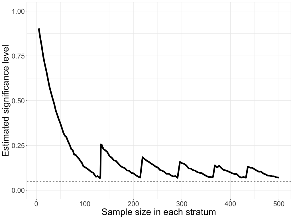
Stratification complicates inference. Texts generally suggest using a stratified version of Student’s -test, approximating the distribution of a weighted sum of stratum-wise sample means by Student’s -distribution [Neyman, 1934, Kish, 1965, Cochran, 1977]. That approximation is good when is approximately normal in every stratum, but the test can be anti-conservative when the within-stratum distributions are skewed. For example, Figure 1 plots the true significance level at various sample sizes of a nominal level 5% stratified -test for a skewed population with two strata. The -test is anti-conservative even when hundreds of samples are drawn from each stratum. The upshot is that for many real-world problems in stratified inference standard methods are invalid: their true level can be greater than their nominal over the class of possible populations to which the problem belongs.
This paper introduces methods to make conservative, non-asymptotic inferences about from stratified samples from bounded populations, without relying on parametric assumptions. The tests are sequentially valid, allowing optional stopping and optional continuation: the analyst may check results as each sample arrives and decide whether to stop sampling or continue gathering data. We call such methods SFSNP-valid (sequential, finite-sample, nonparametric). Audits are our lead example, but the methods are also useful for stratified surveys or blocked randomized controlled trials in many regulatory or scientific applications.
In broad brush, the new method works as follows: the “global” null hypothesis is represented as a union of intersection hypotheses. Each intersection hypothesis specifies the mean in every stratum and corresponds to a population that satisfies the a priori bounds and has mean not greater than . The global null hypothesis is rejected if every intersection hypothesis in the union is rejected. For a given intersection null, information about each within-stratum mean is summarized by a test statistic that is a nonnegative supermartingale starting at 1 if the stratum mean is less than or equal to its hypothesized value—a test supermartingale (TSM). Test supermartingales for different strata are combined by multiplication and the combination is converted to a -value for the intersection null. We explore how the choice of test supermartingale and the interleaving of samples across strata jointly affect the computational and statistical performance of the test.
The next section reviews the literature on inference for ‘nonstandard distributions,’ stratified sampling, sequential sampling, finite-sample inference, and inference in the presence of nuisance parameters. Section 3 introduces notation and foundational concepts including sequential stratified sampling and TSMs. We review how to test intersection hypotheses by combining tests of the individual hypotheses. Section 4.1 presents a basic strategy for stratified inference based on summing independently constructed confidence bounds across strata while adjusting for multiplicity. It is unnecessarily conservative. Section 4.2 describes a sharper approach: union-of-intersections tests. Section 5 defines notions of consistency and efficiency for sequential-stratified inference. We describe ‘oracle’ tests that are theoretically optimal for simple alternatives but cannot in general be constructed explicitly for a composite alternative. We then describe empirical approximations to the oracle bets that can be implemented under the composite alternative. Some of these methods do not scale well, and are not computationally tractable for more than a few strata. We propose general strategies for computation in Section 6. Section 7 compares the efficiency of different strategies via a few simulation studies. Section 8 discusses our results and sketches future directions for research. All code used to implement the methods and run simulations is available at https://github.com/spertus/UI-NNSMs.
2 Background and related work
2.1 Nonstandard distributions and auditing
Methods with guaranteed finite-sample validity for bounded populations have been motivated largely by applications in auditing. Audits typically involve (i) high-stakes decisions with a premium on Type I error control; (ii) bounded, but highly skewed ‘nonstandard’ populations, for which asymptotic methods are inaccurate; (iii) probability sampling under the control of the auditor, including stratified and/or sequential sampling.
Financial audits aim to determine whether the stated value of a set of assets or invoices materially111Materiality is often defined indirectly as an amount that would cause a decision maker to decide differently; in practice, it often taken to be a fixed percentage, e.g., 10%. overstates the total true value [Panel on Nonstandard Mixtures of Distributions, 1988], and to draw inferences about the total overstatement. Large sums of money are often involved. For example, the United States Center for Medicare and Medicaid Services relies on random sampling [US CMS, 2023] to estimate and recover billions of dollars in overpayments [Bittinger et al., 2022]. The populations involved are bounded because the amount by which the value of an asset or the amount of an invoice has been overstated is at most the stated value of the asset or invoice. Stratified random sampling is often employed in financial audits [US DHS, 2020] and may dramatically lower the cost of the audit itself [Fienberg et al., 1977].
Election audits are mathematically similar to financial audits, but with a different notion of materiality: the total error is material if it caused any losing candidate to appear to win. If there is a trustworthy, organized record of the votes (see [Appel and Stark, 2020] for steps to establish whether the record is trustworthy), risk-limiting audits (RLAs) can provide evidence that reported winners of an election really won—or ensure a high probability of correcting the reported results if the reported winners did not really win [Stark, 2008, 2020, 2023]. Stratification is useful in election audits for a variety of reasons, including statutory constraints on how audit samples are drawn.
2.2 Finite-sample and sequential inference
Finite-sample nonparametric inference procedures for fixed-size, unstratified samples from bounded populations have been around for some time. Early versions of such procedures include Hoeffding’s bound [Hoeffding, 1963] for bounded distributions and Anderson’s bound [Anderson, 1967] for nonnegative distributions. These methods found particular use in auditing, where skewness undermines normal-theory inference, but they can be very conservative [Bickel, 1992, Fienberg et al., 1977]. Romano and Wolf [2000] proposed a confidence interval that is conservative and has asymptotically optimal width. A simpler, “empirical Bernstein” bound was derived by Maurer and Pontil [2009]. See also Gaffke [2005] and Learned-Miller and Thomas [2020].
Recent work leverages pioneering results by Ville [1939], Wald [1945], and Robbins [1952] to advance SFSNP-valid inference for unstratified sampling [Howard et al., 2019, Waudby-Smith and Ramdas, 2024, Orabona and Jun, 2022, Stark, 2023]. While Wald [1945] proved the validity of the sequential probability ratio test directly, it is a special case of Ville’s inequality; see also Kaplan [1987]. Essentially every fully sequential method uses TSMs and applies Ville’s inequality [Ville, 1939] to yield an SFSNP-valid -value, from which confidence sets can be derived through the usual duality.
Exponential supermartingales include sequential analogues of the Hoeffding and empirical Bernstein bounds [Howard et al., 2021]. Foundational work on -values (nonnegative random variables with expected value 1 under the null) by Shafer and Vovk [2019] and recent contributions by Waudby-Smith and Ramdas [2024], Cho et al. [2024], and Orabona and Jun [2022] using TSMs to construct confidence bounds have simplified, unified, and sharpened SFSNP-valid inference. Ek et al. [2023] study adaptively reweighted TSMs for intersection hypotheses. This paper extends TSMs to stratified inference.
2.3 Stratification
History and asymptotic inference:
Cournot [1843] showed that for binary populations, stratified sampling with proportional allocation is never less precise than simple random sampling. Tchouproff [1923] derived the optimal stratum sample allocation (for mean squared error) based on stratum sizes and variances, now known as Neyman allocation. Neyman independently built on Tchouproff [1923] in a seminal paper on survey sampling, arguing for random sampling over purposive sampling, which was common at the time [Neyman, 1934, Fienberg and Tanur, 1996]. Neyman [1934] addressed both estimation and inference, including confidence intervals for means of stratified populations. Neyman elsewhere codified strict level control as a basic goal in statistical inference [Lehmann, 1993], but Neyman [1934] suggests that asymptotic normal-theory confidence intervals are adequate for applied problems when the sample is not smaller than 15. Foundational textbooks on survey sampling—including Hansen et al. [1953], Kish [1965], and Cochran [1977]—have promulgated asymptotic tests and confidence intervals for various designs. Those methods can have arbitrarily poor coverage depending on the true population distribution (Figure 1 and Lehmann and Romano [2005]).
Finite-sample stratified inference:
A basic method to construct finite-sample confidence intervals for stratified binary populations combines multiplicity-corrected confidence bounds constructed separately for each stratum [Wright, 1991]. Wendell and Schmee [1996] improved on Wright’s method for binary populations by testing the composite hypothesis using as the -value the maximum -value over the simple hypotheses whose union comprises the composite hypothesis. The method of Wendell and Schmee [1996] is intractable when is large.
Stratified inference and nuisance parameters:
Inference about population means and totals from stratified samples can be viewed as problems with nuisance parameters, where is the number of strata. One approach to testing when there are nuisance parameters is to maximize the -value over all possible values of the nuisance parameters or over a confidence set for the nuisance parameters [Tsui and Weerahandi, 1989, Berger and Boos, 1994, Silvapulle, 1996]. Maximizing the -value over the nuisance parameters is equivalent to partitioning the null hypothesis into a union across all possible values of the nuisance parameters that yield the hypothesized value of the parameter of interest—a union of intersections—then testing every element of the partition and rejecting the union if and only if every simple hypothesis in the union is rejected.
That approach was taken by Ottoboni et al. [2018] (SUITE) for sequential inference in election audits and by Stark in 2019222See https://github.com/pbstark/Strat. for inference about stratified binary populations from fixed-size samples. SUITE used Fisher’s combining function to pool evidence across strata. Stark [2020] generalized SUITE. Stark [2023] proposed using union-of-intersections tests with product combining of TSMs for SFSNP-valid inference in stratified risk-limiting audits. Spertus and Stark [2022] investigated sample sizes for a range of combining functions, TSMs, and selection strategies for stratified comparison audits. Cho et al. [2024] use betting TSMs for best arm identification and other hypotheses of interest in multi-armed bandits. Their method tests composite hypotheses about means of multiple data streams under adaptive sampling and could be applied to stratified sampling. We suspect their use of averaging to combine -values and their particular betting rule may reduce statistical efficiency compared to the methods for sequential stratified inference presented here.
The present contribution can be viewed as a set of methods for rigorous inference in a nonparametric problem with a multi-dimensional nuisance parameter.
3 Preliminaries and notation
3.1 Population and parameters
We use calligraphic font for sets and bags, and bold font for vectors (and sometimes for tuples). Tuples are denoted using parentheses, e.g., ; finite-dimensional vectors are denoted using square brackets, e.g., . If and are two vectors with the same dimension , we write iff , ; and we define the dot product . The vector of all zeroes is and the vector of all 1s is , with dimension implicit from context. The set of nonnegative integers including 0 is . If is a set or a bag, then is its cardinality. For two scalars and , is their minimum and is their maximum.
The population of interest is a bag of real numbers . The development below takes to be a finite population, with , but the results apply with few changes when is countable or uncountably infinite. As noted above, only one-sided bounds on the population are needed to get one-sided confidence bounds or one-sided tests; however, for simplicity of notation, we assume that each element of the population is in .333Any known lower bound on elements can be accommodated by shifting: if then . If all the elements have the same upper and lower bounds and , they can be rescaled to with an affine transformation ; the mean of the resulting population is the same affine transformation applied to the original mean. The population mean is , and we want to test the global null hypothesis:
| (1) |
for global null mean . A lower confidence bound is the largest for which is not rejected at level . If there are upper bounds for each element of the population, an upper one-sided test can be obtained by subtracting each element from its upper bound and then using a lower one-sided test, mutatis mutandis.
Let denote the vector of stratum sizes. The symbol denotes a generic stratified population, a tuple of bags with items in the th bag, , so that . The symbol denotes the true, unknown population. The symbol represents all -tuples of bags of numbers in such that the th bag, , has items; that is, denotes all stratified -valued populations with the requisite number of items in each stratum. We use to denote a generic element of the th stratum, e.g., . The vector of stratum-wise means for population is ., where . The vector of stratum weights is , where . The mean of a stratified population is
Let denote the set of null populations; the global null hypothesis can be written . Also let denote the set of alternative populations. Together, and partition .
Let be the true global mean, and be the true stratum-wise means. An intersection null hypothesis is the assertion
for the intersection null mean . In words, the intersection null hypothesis posits that each stratum-wise mean is below a corresponding stratum-wise null mean . The global null hypothesis can be written as a union of intersection null hypotheses:
| (2) |
where
| (3) |
is the set of all intersection nulls for which the global null is true444If there are constraints on the support of each stratum (e.g., that each element is 0 or 1), that information can be used to sharpen inferences. See Section 4.2.1 below..
3.2 Sampling design
We consider samples drawn uniformly at random within strata, with or without replacement; generalizing to sampling with probability proportional to a measure of “size” is straightforward [Stark, 2023]. Recall that a fixed-size stratified sample consists of independent (unordered) samples , where the sample from stratum , , is drawn by uniform random sampling with or without replacement. When draws are with replacement, the data are IID uniform draws from . When draws are without replacement, is uniform over all subsets of size from .
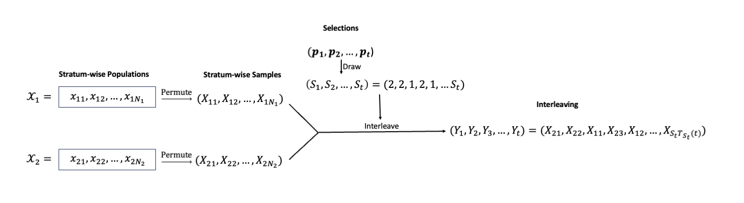
Sequential stratified samples.
Unlike fixed-size stratified samples, sequential stratified samples have an order within and across strata, which necessitates a more detailed specification. Let be a sequence of random variables representing the samples drawn sequentially from stratum . For sampling without replacement, can run from 1 to and is a random permutation of the stratum values . For sampling with replacement, runs from 1 to and the elements of are IID. Regardless, the variables are exchangeable for each and the sequences and are independent of each other for .
An interleaving of samples across strata is a stochastic process indexed by “time” ; is the -prefix of . Each interleaving is characterized by a stochastic process, the stratum selection : the item in the th position in the interleaving comes from stratum . Let . The variable must be predictable—it can depend on past data but not on for —and may also involve auxiliary randomness. We emphasize that does not depend on , and is observed before is observed: is the stratum from which the th sample will be drawn. For , let
| (4) |
and set , . Naturally, for each , and . If for each , has one component equal to 1 and the rest equal to zero (i.e., is one-hot), the stratum selection is deterministic (conditional on the past). We refer to as the stratum selector. To summarize, the stratum selection is a stochastic process taking values in , while the stratum selector is a vector-valued stochastic process taking values in that specifies the chance that the next draw will be from each of the strata, given the sampling history so far.
As of time , the number of items in the interleaving that came from stratum is , and are the data from stratum . Thus, the th item in the interleaving,
is the th item drawn from stratum , so . The hypothesis tests we consider use samples from each stratum in the order in which those samples are drawn, but tests of different intersection nulls may use different interleavings.
3.3 SFSNP-valid hypothesis tests
We will construct SFSNP-valid tests of the global null , i.e., .
Definition 1 (SFSNP-valid -value).
Let be a -valued stochastic process. Then is an SFSNP-valid -value for the global null hypothesis if for all ,
If is an SFSNP-valid -value, then rejecting the null hypothesis if for some is a SFSNP-valid hypothesis test with significance level . The random variable is the stopping time of the test.
Finding SFSNP-valid tests such that the expected value of is small when the global null is false is the primary goal of this paper. Minimizing (expected) stopping times for sequential tests is analogous to maximizing power in the usual fixed-sample, Neyman-Pearson theory of testing. We return to this idea in Section 5, where our primary concern is efficient SFSNP-valid tests of .
3.4 Test supermartingales
In recent years, martingales—fundamental objects in probability theory with close connections to betting—have been used to construct efficient sequential tests and confidence intervals. One can construct an SFSNP-valid -value from any statistic that is a nonnegative supermartingale starting at 1 when is true; such statistics are called test supermartingales [Shafer et al., 2011]:
Definition 2 (Test supermartingale (TSM)).
The stochastic process is a test supermartingale (TSM) for with respect to the stochastic process if, when is true, is a nonnegative supermartingale and .
TSMs yield SFSNP-valid -values through the following special case of a result of Ville [1939]:
Proposition 1 (Ville, 1939).
Let be a TSM for . Then for all and any
Ville’s inequality is analogous to Markov’s inequality, but holds uniformly over , allowing sequentially valid inference. The reciprocal of the running maximum of a TSM, , is an SFSNP-valid -value.
3.4.1 Constructing TSMs from random samples
We start by considering a single stratum, . The within-stratum null mean is . We construct a process that is a TSM with respect to for the stratum null . Recall that is the sample size from stratum at time . The conditional stratum-wise null mean is the implied mean of the values remaining in at time if , given that we have already observed . For sampling with replacement, . For sampling without replacement,
A generic form for a within-stratum TSM is
where is any term such that when . We will use statistics of the form
which defines as a betting TSM. Waudby-Smith and Ramdas [2024], Orabona and Jun [2022] show that for suitable choices of (which can be thought of as a normalized bet), betting martingales provide sharper inferences than many other options for , such as exponential supermartingales [Howard et al., 2021]. The TSM for stratum at time can be written:
Within-stratum TSMs can be combined to form a -value for an intersection null.
3.4.2 Intersection test supermartingales (I-TSMs)
Consider a particular intersection null . Define the intersection TSM (I-TSM):
where is the th term of the within-stratum TSM for stratum . By commutativity, the I-TSM at time can be written as an interleaving of terms from the within-stratum TSMs, where the (possibly random, but predictable) interleaving is defined by the selections . Because the selections are predictable, the I-TSM is indeed a TSM for :
The third equality holds because samples from different strata are independent, and the inequality in the fourth line holds by construction of the within-stratum TSMs paired with the fact that under the intersection null. (That the I-TSM is an -value also follows from the fact that it can be written as a product of independent -values. See, e.g., Vovk and Wang [2021].)
The reciprocal of the running maximum,
is a sequentially valid -value for the intersection null . If an I-TSM uses betting TSMs in every stratum, it is a betting I-TSM.
4 Stratified inference with TSMs
In this section, we describe two methods for stratified inference that leverage I-TSMs. The first is a weighted sum of TSM-based, sequentially valid lower confidence bounds for the stratum-wise means. This is akin to Wright’s method for conservative stratified inference on binary populations [Wright, 1991]. We show that (perhaps surprisingly) using TSMs avoids the need to explicitly adjust for multiplicity. The second method forms an I-TSM for every intersection null and takes the smallest. The second method is trickier to implement, but has less slack than the first method.
4.1 Simple stratified inference: combining confidence bounds
We use a linear combination of independent sequentially valid lower confidence bounds (LCBs) for the stratum-wise means to form a sequentially valid LCB for . The weights in the linear combination are the stratum weights . If the linear combination is above the global null mean, the test rejects. For a level global test, the individual LCBs must be simultaneously valid at level , controlling the family-wise error rate. If each LCB were generic, we might use the Šidák correction for independent tests, constructing each LCB at level . This incurs a steep penalty as increases, almost the penalty of the Bonferonni correction.
However, we are basing each LCB on a TSM. The following lemma, proved in Section B.1, shows that using a TSM in each stratum obviates the need to adjust for multiplicity.
Lemma 1 (Validity of TSM LCBs).
For each stratum , define the sequence where
Then:
-
1.
are separately sequentially valid lower confidence bounds, in the sense that whenever :
-
2.
are simultaneously sequentially valid lower confidence bounds, in the sense that whenever :
The first result simply states that we can construct confidence bounds from TSMs, which follows immediately from the duality of tests and confidence sets [Lehmann and Romano, 2005], as used extensively in [Waudby-Smith and Ramdas, 2024]. The second, stronger result follows from the closure principle of Marcus et al. [1976], which was employed by Vovk and Wang [2021] to adjust -values for multiplicity. Surprisingly, LCBs constructed from TSMs are simultaneously valid without the need for an explicit multiplicity correction.
Proposition 2.
Let be a LCB constructed from a TSM with samples from stratum at time , . Consider the stratum-weighted sum
Since are simultaneously and sequentially valid LCBs for , whenever ,
Thus is an SFSNP-valid LCB for , and a test that rejects when is an SFSNP-valid level test with stopping time .
The proof is contained in the theorem statement; the final step applies Lemma 1. This approach is easy to implement when computing the LCBs is straightforward and efficient; Waudby-Smith and Ramdas [2024] and Orabona and Jun [2022] describe a number of possibilities. The selection rule will influence the efficiency of the bound.
There are two sources of slack in using Proposition 2 to test . One is due to the second inequality in Proposition 2: the LCB method bounds each of the components of separately, but we only need to bound . The other source of slack is in controlling for multiplicity using closed testing, which requires each of the TSMs to reach . In contrast, to test the intersection null , we only need the product of the stratum-wise TSMs to reach . In particular, the test could reject with all TSMs equal to , a lower hurdle in every stratum. We now develop a test that avoids these two sources of slack.
4.2 Union-of-intersections test sequence (UI-TS)
Definition 3 (Union-of-Intersections Test Sequence).
A stochastic process is a Union-of-Intersections Test Sequence (UI-TS) for the composite null hypothesis if for all ,
Equivalently, is a UI-TS if its truncated reciprocal is an anytime-valid -value for the null .
A UI-TS need not be a supermartingale under (below, we construct UI-TSs as the minimum across I-TSMs that involve incommensurable filtrations), but it is an -process [Shafer, 2021, Vovk and Wang, 2021, Ramdas et al., 2023, Grünwald et al., 2024].
Recall the union-of-intersections form of the global null in Equation 2 and the definition of in Equation 3. As shown in Section 3.4.2, we can test a particular using an I-TSM. We can reject if the -value for every is less than , i.e., if the smallest I-TSM evaluated over is at least . Therefore,
| (5) |
is a UI-TS for . When every is a betting I-TSM, is a betting UI-TS.
4.2.1 The boundary of
We shall consider only betting UI-TSs based on TSMs that are monotone decreasing in for each , so that the I-TSM is componentwise monotone in . As a result, the minimum of occurs on the boundary of . The boundary depends on the support of each stratum population, which in general will be unknown.
Specifically, let be the set of all possible means in stratum . For example, if stratum is binary, then . Let be the Cartesian product of all possible stratumwise means . The boundary of is
For the TSMs we consider,555For the TSMs we consider, if , then there is some point with for which we enforce that uses the same selections and bets as . As result, for all because of the monotonicity of the stratumwise TSMs in . the value of that minimizes is in . Futhermore, define
| (6) |
Because of the componentwise monotonicity, optimizing over the set rather than gives a conservative result. In what follows, we will generally define . The set is a polytope, the intersection of the -cube with the hyperplane . The geometry of is important for the computational tractability of some UI-TSs (see Appendix C).
4.2.2 Global stopping time and global sample size
We distinguish between the stopping time of a UI-TS and its workload measured by the number of samples it requires to stop. To do so, we embellish the notation to highlight dependence on the intersection null . For each , denote the selections by , the selection rule by , and the stratum-wise sample sizes by . The stopping time of the level test induced by UI-TS at is
This is the number of samples needed to reject intersection null using the constituent I-TSM , and the quantity is the number of samples needed from stratum . The global stopping time is the sample size needed for the “last” I-TSM, considered on its own, to hit or cross :
On the other hand, the global sample size is the total number of samples drawn across all strata when is rejected:
Because is the sum of stratumwise maxima, . However, for a broad class of tests , for instance, when the selections do not depend on . Below, when is clear from context, we will drop it from the notation.
5 Desirable properties: consistency and efficiency
This section defines consistency and efficiency for sequential stratified inference.
5.1 Consistency
Loosely speaking, a test is consistent if, with probability 1, it eventually rejects the global null when the global null is false. We first define consistency for intersection nulls, then for the global null.
Definition 4 (Intersection consistency).
Consider a sequentially valid, level test of the intersection null hypothesis , and let denote the -value for that test at time . If
for all such that , then the test is intersection consistent for .
An intersection consistent test can be constructed from an I-TSM that, with probability 1, grows without bound whenever . An I-TSM is consistent if it leads to an intersection consistent test of . Constructing such an I-TSM requires protecting against two failure modes. First, we must ensure that in at least one stratum in which , the stratumwise TSM grows.666Recalling a classic example, suppose that in each stratum the population is binary and we are using the Bernoulli SPRT as the TSM. It is well known that, even when , if the tuning parameter corresponding to the suspected alternative mean is incorrectly specified, the stratumwise TSM has a positive probability of never crossing . Predictably estimating the true mean or mixing over a prior distribution can remedy this issue (c.f. [Robbins, 1952, Stark, 2023, Waudby-Smith and Ramdas, 2024]). Second, we must ensure that the stratumwise TSM for any stratum in which (eventually) does not drive the I-TSM towards zero. That can be accomplished by curtailing sampling in strata where there is evidence that ; by reducing the bets in those strata to zero; or by ensuring that at some stage, an overwhelming fraction of the samples come from some stratum in which the null is false.777Instead of combining stratumwise TSMs by multiplication, we could combine them by averaging [Cho et al., 2024]; or instead of combining stratumwise TSMs into an I-TSM, we could combine the (independent) stratumwise -values derived from the TSMs into a single -value, for instance, using Fisher’s combining function [Ottoboni et al., 2018, Spertus and Stark, 2022].
Definition 5 (Global consistency).
Consider a sequentially valid, level test of the global null , and let denote the -value for that test at time . The test is globally consistent iff
whenever .
A globally consistent test is a test of power 1 [Robbins and Siegmund, 1974]. For a UI-TS using I-TSMs that are monotone in ,
We will call a UI-TS inconsistent if the test based on it is inconsistent. If every -value in the set is intersection consistent, the UI-TS is consistent. In theory, we can use any set of consistent I-TSMs to construct a consistent UI-TS in this way. In practice, may be uncountably infinite, so maximizing over may be intractable unless has special structure.
Inconsistent tests:
Consider a UI-TS with fixed selections and bets constant across nulls, strata, and time. When the bets and selections are fixed across the set of I-TSMs is log-concave over (see Section C.2), so the minimum I-TSM occurs at a vertex of the polytope . Let denote the set of vertices of . For instance, if and , . It follows from log-concavity that a UI-TS with fixed bets and selections is consistent if and only if with probability 1, it eventually rejects all .
Consider testing the null and suppose the population consists of two strata of the same size, each comprising the point mass for all and . Under , any sample from stratum 1 yields
while a sample from stratum 2 yields
After draws from stratum 1 and draws from stratum 2, the I-TSM will equal
For to reach requires there to be some for which
Conversely, , so to reject requires there to be some for which
Round-robin selection implies for all . In that case, both inequalities cannot be satisfied when is small, and the UI-TS is inconsistent.
A simple consistent strategy is to sample from a single stratum (by symmetry the choice of stratum is irrelevant) until one vertex is rejected (at which point, the I-TSM for the other vertex may have a value close to 0), then sample from the other stratum until the second vertex is rejected, which will require building the gambler’s fortune back from near ruin.
This construction suggests a more general recipe for a consistent UI-TS. If the alternative is true, every intersection null is false in at least one stratum. Fix the bets and test each in turn, sampling from the stratum until that null is rejected, then continuing to the next . (Data already observed cannot be discarded when testing the next vertex.) If the I-TSM for that will grow for any sample from stratum for any bet and any stratum-wise population . Thus if all have for some , this method yields a consistent test for sampling with replacement. The situation is more delicate when some vertex does not have a component equal to 0. For example, when and , the vertices are and . Sampling from stratum 1 to test may not be consistent for all bets and populations, e.g., for stratum-wise Bernoulli distributions. Indeed, a betting TSM corresponds to the Bernoulli SPRT [Stark, 2023], and Wald [1945] shows that the Bernoulli SPRT can be inconsistent when the a priori alternative (i.e., the implied bet) is is not the actual value.888We conjecture that, for any true stratum mean , the easiest alternative to reject is a point mass, while the hardest is Bernoulli. For fixed , these are the minimum and maximum variance distributions on , respectively. Moreover, even when it is possible to construct a consistent UI-TS, consistency is a very weak requirement: a UI-TS may be consistent while requiring an impractically large sample size . A stronger criterion is needed.
5.2 Efficiency
The global composite alternative does not completely specify the population, only its mean. In contrast, a simple alternative completely specifies the population . An efficient test keeps small in some sense. In general, no method is best for all ; moreover, is random. One could minimize a summary of the distribution of sample sizes for different , for instance, the supremum (over ) or a weighted average expected sample size. One might also define admissibility with respect to some summary of sample size. For example, we might define a test to be inadmissible with respect to expected sample size if there is a second test such that for every the expected sample size of the second test is not greater than that of the first test, and there is some for which the expected sample size of the second test is strictly less than that of the first test.
To construct tests that perform reasonably well in practice (but which are not in general admissible), we begin by constructing tests that minimize for a simple alternative . Such tests are called Kelly optimal (for the alternative ). We construct Kelly optimal I-TSMs and UI-TSs, which maximize the expected log growth under the alternative; by Wald’s identity [Wald, 1944], that minimizes their expected stopping times . Since for any test, the expected stopping time of a Kelly optimal test is a lower bound on the optimal expected sample size. Furthermore, when the selections are fixed across , we have , and the Kelly optimal UI-TS directly minimizes the expected sample size.
We characterize (a) Kelly-optimal strategies for known simple alternatives; (b) approximately Kelly-optimal for unknown simple alternatives; and (c) computable approximations to (b). Kelly optimality is a target we hope to approximate with predictable, computationally tractable strategies. The computations are dramatically simpler when selections are restricted to be fixed across , i.e., when , in which case the Kelly optimal test minimizes the expected sample size.
5.2.1 Defining efficiency
The simplest definition of efficiency is efficiency at a point: it is the ratio of the expected sample size of the test that minimizes the expected global sample size when to the expected sample size of the test in question when .
Definition 6 (Efficiency at ).
Consider testing the composite null . Given two UI-TSs for , and , the relative efficiency of to at (for expected sample size) is
The efficiency of a test at is its efficiency relative to any level- test that minimizes the expected sample size.
Another metric of test performance is regret, the difference between the expected sample size and the expected sample size of the best method.
Definition 7 (Regret at ).
Consider testing the composite null . Let be any UI-TS for . Its regret at is:
where is any test that minimizes the expected sample size at .
For a fixed alternative, minimizing regret and maximizing efficiency are equivalent, but the minimax procedure that minimizes the maximum regret over a set of alternatives is in general different from the procedure that maximizes the minimum efficiency. Efficiency is a common metric in statistics [Wasserman, 2004, Lehmann and Romano, 2005, Wald, 1945], while regret is more common in computer science and especially in the multi-armed bandit literature [Lai and Robbins, 1985, Berry and Fristedt, 1985, Auer et al., 2002]. Savage [1951] proposed minimax regret (which he called “loss,” in distinction to “negative income”) as a less pessimistic risk measure than the criterion explicitly considered in Wald’s pioneering work on decision theory [Wald, 1950]; Savage [1951, p. 65] points out that Wald’s theory includes minimax regret implicitly [Wald, 1950, p. 124]. The distinction between minimizing loss and minimizing regret is equivalent to that between the REGROW and GROW criteria for -values [Grünwald et al., 2024]. We shall use efficiency primarily.
Sometimes efficiency can be computed or bounded theoretically. For instance, Wald [1945] proves that the SPRT essentially minimizes the expected sample size for testing a point null against a point alternative (for any pre-specified sequential sampling design; in particular, for the stratified case, stratum selection cannot be adaptive). In other words the SPRT is efficient. Wald derives a general formula for for the SPRT. But finding the expected sample size of a UI-TS analytically is intractable even for basic parametric alternatives (e.g. binomials) and simple betting and selection rules (e.g. round-robin selection and fixed bets ). With few exceptions, we use simulation to assess efficiency.
The definition of efficiency can be generalized in at least two ways. First, while Definition 6 considers a simple alternative , we could summarize efficiency over the composite alternative . There are two standard approaches. (1) Summarize the efficiency by a weighted average over the composite alternative (the weights might correspond to a Bayesian prior on the alternative). This is analogous to the GRO criterion in Grünwald et al. [2024]. (2) Summarize performance by the minimum efficiency or the maximum regret over the composite alternative. This is analogous to the REGROW criteria of Grünwald et al. [2024]. A second generalization is to use a functional of the distribution of other than its expected value. For example, efficiency could be defined with respect to the 80th percentile of . Such a definition would bring sequential efficiency more in line with the traditional, fixed-size notion of power, reflecting the sample size at which the test has a high probability of rejecting the null. While stopping-time percentiles can be estimated by simulation, efficiency with respect to expected sample size is more amenable to analysis and optimization.
5.2.2 Kelly-optimality and efficiency
Wald’s equation [Wald, 1945]
can be used to relate Kelly-optimal and efficient tests. Specifically, because a Kelly-optimal test for the alternative maximizes , it minimizes . Kelly-optimal tests are efficient (for sample size) when , including the subclass of UI-TSs with selections fixed across . Furthermore, the expected stopping time of the Kelly-optimal test is a lower bound on the expected sample size of an efficient test.
5.2.3 Kelly optimality for a composite null and simple alternative
Definition 8 (Kelly-optimal betting UI-TS).
A betting UI-TS for the composite null is Kelly-optimal for the simple alternative if its expected log-growth under that alternative is maximal over the class of all betting UI-TSs for . That is,
where . The expectation is taken with respect to random sampling from and the stratum selections .
We show below how to construct a Kelly-optimal UI-TS; there may be more than one. We first define Kelly-optimality for an I-TSM for the intersection null with respect to a simple alternative.
Definition 9 (Kelly-optimal betting I-TSM).
A betting I-TSM for the intersection null is Kelly-optimal for the simple alternative if its expected log-growth is maximal among all betting I-TSMs for :
where
is the change in the I-TSM at time . The supremum is over all choices of bets and selection rules that yield an I-TSM for . The expectation is with respect to the random sampling from and the stratum selections .
We now construct a Kelly-optimal betting I-TSM by finding the Kelly-optimal bets and selection rules that parameterize . The optimal bets do not depend on the selection rule . Lemma 2, proved in Section B.2, yields a Kelly-optimal I-TSM.
Lemma 2 (Constructing a Kelly-optimal I-TSM).
Fix an intersection null and a simple alternative .
-
1.
Bets: Define the bets
where each
-
2.
Selection rules: Let be the set of strata with maximal expected log-growth under the alternative for the bets . Define the selection rule
where
The I-TSM that uses and is Kelly-optimal.
If the sampling is with replacement (the draws from each stratum are IID), then the Kelly-optimal bets and selection rules do not depend on .
Lemma 3 (A Kelly-optimal UI-TS).
Fix a simple alternative . For each , let be the Kelly-optimal I-TSM for characterized by the bets and selections in Lemma 2. The UI-TS
is globally Kelly-optimal for .
That Kelly-optimal UI-TS is parameterized by the entire set of intersection Kelly-optimal bets and selection rules . The proof of Lemma 3 is essentially self-evident: any TSM under is of the form ; we can always maximize the growth of the minimum by maximizing the growth of every I-TSM in , which is achieved by using the Kelly-optimal strategy for every . Even when is known, it is difficult to explicitly construct a Kelly-optimal UI-TS, except in simple cases. We give such an example in Appendix A, where the population consists of two point-mass strata ( for all ). For more general simple alternatives, could be constructed numerically, but not when the alternative is composite. We now describe a strategy that achieves efficiency by “learning” aspects of that allow bets and selections to approximate the Kelly-optimal solution.
5.2.4 Approximate Kelly optimality under the intersection-composite alternative
Consider again a fixed intersection null and the intersection-composite alternative . Within stratum , the alternative is not specified, so we cannot directly apply Lemma 2. Instead, we use a predictable betting method that approximates the Kelly-optimal strategy using past data, “approximate growth rate adapted to the particular alternative” (AGRAPA) [Waudby-Smith and Ramdas, 2024]. Within stratum , the AGRAPA bet is
where and are the lagged empirical mean and variance, and is a user-specified truncation parameter. When the empirical mean is above the null mean and the variance is relatively small, AGRAPA bets more aggressively: the data give confidence that the next draw will be above . The truncation at 0 ensures the bet is 0 in strata where the empirical mean is below the null; the truncation at prevents bets from becoming too aggressive ( ensures that for all ). Using AGRAPA bets in each stratum provides a fairly efficient betting strategy under and the intersection-composite alternative.
The multi-arm bandit literature offers a range of potential options for . For example, we could pull from the stratum with the largest upper confidence bound on (a UCB algorithm [Lai and Robbins, 1985]) or according to a posterior probability that is largest for an assumed prior (a Thompson sampling algorithm [Thompson, 1933]). All of these strategies approximate the Kelly-optimal solution.
5.2.5 Other betting strategies
We propose two additional betting strategies that, when paired with fixed stratum selections , are more tractable computationally than AGRAPA and other approximately Kelly-optimal bets. We present the strategies now and theoretically bound their stopping times for stratified point-mass populations, wherein . We discuss their computational properties in the next section.
The first strategy uses the same bet for all :
The bet may vary over time as a predictable function of past data, but the bets must be identical for every I-TSM . The predictable plug-in strategy recommended by Waudby-Smith and Ramdas [2024]
is an instance of a fixed bet (truncated to rather than ).
The second strategy is
where is a predictable tuning parameter, and the ”I” superscript stands for inverse. An inverse bet is valid as long as and .
To define , note that for any given null , it is sensible to bet more when the true mean is larger and the standard deviation is smaller. This suggests setting
where and are predictable estimates of the true mean and standard deviation. We recommend setting them to be the lagged sample mean and sample standard deviation, though regularized or Bayesian estimates are also possible (as in, e.g., Stark [2023]). The limits are user-chosen truncation parameters ensuring the bets are valid. As defaults, we recommend setting and so that some amount is always wagered and the gambler does not “bet the farm” and go broke (i.e., to ensure that for all ).
6 Computation
The results of Section 5.2.4 in principle allow one to construct an approximately optimal I-TSM for every ; Lemma 3 then suggests an efficient UI-TS under the global-composite alternative . In practice, this is computationally infeasible.
The computational tractability of a UI-TS depends on how the constituent I-TSMs are constructed and in particular how they depend on . We classify I-TSMs accordingly. The term -aware refers to betting and selection strategies that depend on ; -oblivious refers to strategies that do not. Similarly, a predictable strategy is adaptive if it explicitly depends on past data, and nonadaptive otherwise. A strategy may be adaptive but -oblivious, non-adaptive but -aware, etc. The strategies proposed in Section 5.2.4 are adaptive and -aware. A UI-TS is called -oblivious only if both the stratum selectors and bets are -oblivious.
Small , small , discrete support:
Recall from Section 4.2.1 that is the (possibly finite) boundary of . If the support of is small and known (e.g., if is known to be binary), if there are few strata (e.g., ), and if the strata are small (e.g., ), it is feasible to enumerate . That makes it feasible to use an arbitrary -aware strategy by brute-force minimization over . We discuss the complexity of enumerating in Appendix C.
Small :
When the strata are large or when the support is unknown, it is not possible to minimize over by brute force. In Section C.2 we show that the I-TSM is log-concave over when the bets and selections are -oblivious. As a result, when bets and selections are -oblivious over a convex subset of , the I-TSM is log-concave over that subset, so the minimum must be attained at an extreme point of that subset. That suggests a strategy for finding the global minimum: partition into convex subsets within each of which the bets and selections are -oblivious, find the minimum over each subset by exploiting the log-concavity, then find the minimum of those minima.
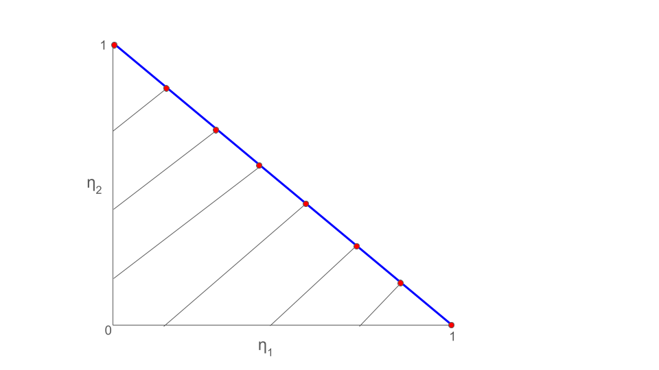
This strategy is illustrated in Figure 3, which partitions the regions into convex bands and evaluates the I-TSM at their vertices. It requires specifying bets and selections . The number of I-TSM evaluations required depends on the number of bands that share each vertex. The betting and selection rule for band can be chosen to optimize performance at some point in the band, for instance, the centroid of the intersection of the band with . We focus on the case , in which case the bands can be defined by points along the line . The size of the bands affects the efficiency of the UI-TS. Below, we choose the bands using an equispaced grid. We do not evaluate this method for because we expect it to scale poorly in : the resolution decreases as increases with fixed.
Moderate :
The coarsest banding strategy is , which yields an -oblivious approach with the same bets and selections for every . The resulting I-TSM is log-concave in over all of . Its minimum is attained at a vertex of the polytope : we can compute by evaluating at the vertices . The number of vertices is combinatorial in , as when is even and stratum-sizes are equal. Enumerating the vertices is tractable for any and any support if the number of strata is not too big (e.g. ).
Arbitrary :
If we use -oblivious selections , the -aware inverse betting strategy leads to an I-TSM that is smooth and log-convex in (see Section C.3). The minimum generally occurs on the interior of and can be found numerically: the objective and constraints are convex, so projected gradient descent can find the UI-TS for arbitrary and . Computation times for log-convex UI-TSs and the LCB method are compared in Section C.4.
7 Simulations
This section examines the efficiency of the proposed methods in three simulation studies. The first study involves point masses within strata, an idealization of some common auditing populations, wherein the vast majority of values are concentrated at a single point reflecting correctly reported values, with a thin left tail corresponding to erroneous values. Point masses are analogous to error-free audit populations. The second study involves binary populations with varying , the fraction of 1s in stratum . The third uses Gaussian superpopulations within strata, truncated to , modeling applications to continuous bounded populations (e.g. soil organic carbon measurement [Stanley et al., 2023]).
7.1 Point-mass simulations
We evaluated methods on populations with stratum sizes and point masses as within-stratum distributions, so that for and . True global means ranged from 0.51 to 0.75, and differences between stratum means were 0 () or 0.5 ().
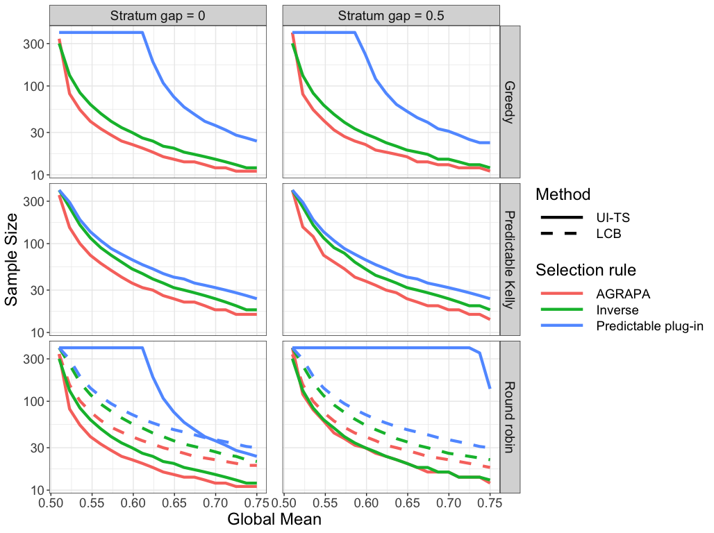
We computed LCBs as in Section 4.1 and UI-TSs. The banding strategy discussed in Section 6 was used with bands on an equally spaced grid. Bets were AGRAPA (Section 5.2.4), -oblivious predictable mixture (Section 5.2.5), or inverse (Section 5.2.5). The selection rule was -oblivious, nonadaptive round robin, an -aware and adaptive “predictable Kelly” strategy using a UCB-style algorithm on every , or an -oblivious “greedy” strategy using the UCB-style algorithm iteratively on the previously minimizing (the minimizer at time ) to produce a single selection for all I-TSMs. In more detail, the UCB-style methods worked as follows: for each , each stratum , and each time , the predictable Kelly strategy computed the average of the past TSM terms and the standard error of that average , estimated as the sample standard deviation of the terms divided by . For each , an upper confidence bound on the expected gain was computed as , and the next sample was drawn from the stratum with the largest upper confidence bound. This predictable Kelly strategy was only implemented for the UI-TSs, since the LCB approach cannot use -aware selection strategies. The greedy strategy was similar, but instead of using the UCB-algorithm to select a sequence for each , it implemented the UCB-algorithm for (the most recent minimizer) and applied that choice to the selections for every . The greedy strategy is -oblivious since it results in a single selection sequence .
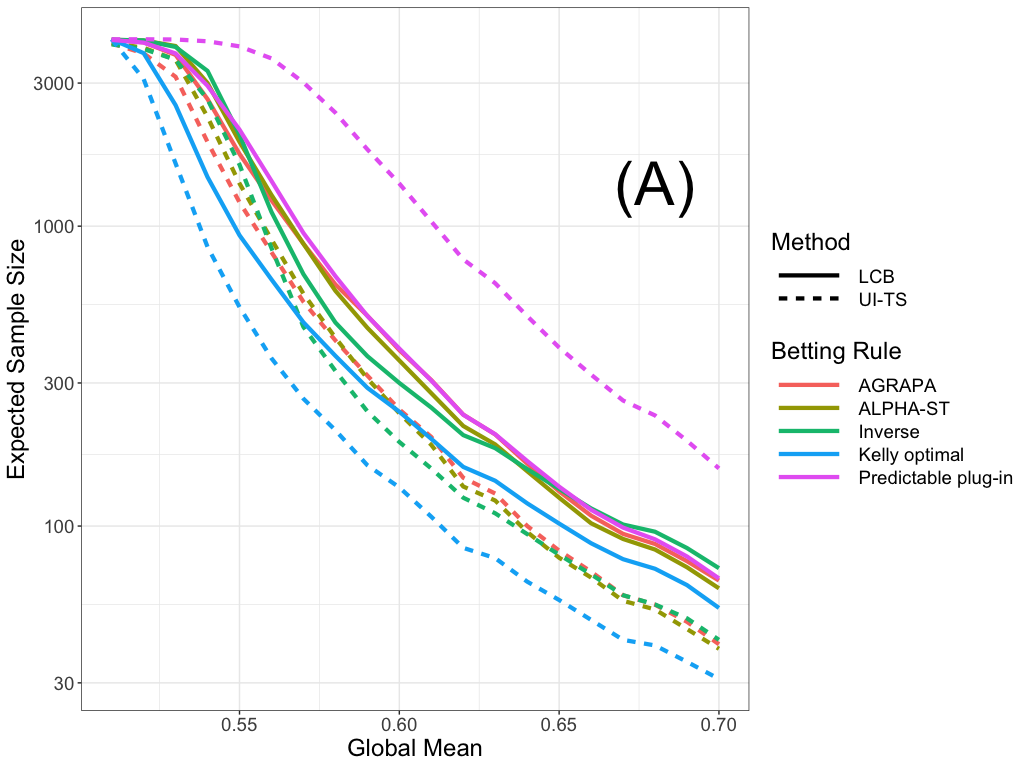
We ran each combination of inference method, betting strategy, and selection strategy on each population and recorded the (deterministic) stopping time. Because the populations are point masses, there is no randomness in sampling and the sample sizes only needed to be computed once. The sample sizes (averaged across populations and selection rules) for UI-TSs with AGRAPA bets at various appear in Table 1. The efficiency of the UI-TS banding strategy increases as increases, as does the computation time. In this case, the efficiency gains level off around . Sample sizes at appear in Figure 4. UI-TSs are generally more efficient than LCBs, and the performance gap can be substantial (the y-axis is on the log scale). The exception is when neither the bets nor the selections are -aware. In particular, LCBs performed better when predictable plug-in bets were used. UI-TSs were much sharper with AGRAPA or inverse bets. However, -oblivious selections led to lower sample sizes than the -aware predictable Kelly rule. Despite having approximately optimal stopping times, the predictable Kelly rule led to poor sample sizes because different selections were used for each intersection null. Greedy selection was better than round robin when used with AGRAPA or predictable plug-in bets, in particular when the stratum means differed ().
| Sample size () | Run time (s) | |
|---|---|---|
| 1 | 400.0 | 0.2 |
| 3 | 179.7 | 0.6 |
| 10 | 90.1 | 1.8 |
| 100 | 48.3 | 17.4 |
| 500 | 46.8 | 87.8 |
7.2 Bernoulli simulations
We created 2-stratum populations of size from Bernoulli distributions with stratum-wise success probabilities or , with population means ranging from 0.51 to 0.74. We tested the global null against these alternatives and recorded the sample sizes for the methods described in Section 7.1. For this simulation we added two new betting strategies based on Kelly optimality for Bernoulli populations. Within each stratum, the “shrink-trunc Bernoulli” strategy took the mean estimate described in Section 2.5.2 of Stark [2023],999The notation in Stark [2023] is essentially flipped from ours. It uses for our (the alternative mean estimate) and for our (the null mean). and transformed it into a bet as described in Section 2.3 of that paper. In detail, the a priori estimate of the alternative was set at for each stratum and null mean, the anchoring factor was so that the sample mean quickly dominates the estimate, and the estimate was truncated to be no less than . That mean estimate was transformed to a bet by taking
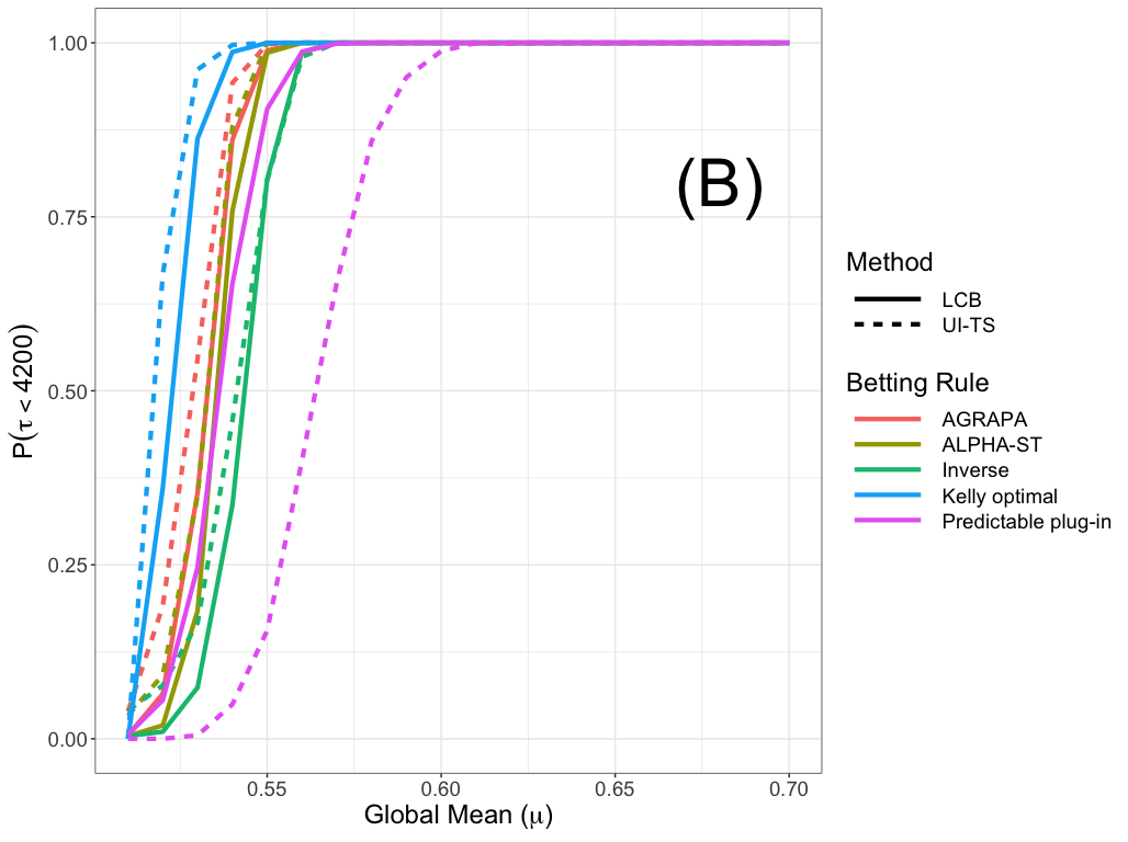
This is like using the Bernoulli SPRT [Wald, 1947] but instead of using a fixed alternative, using a predictable estimate for the alternative. We also tried the true alternative mean in each stratum, yielding the Kelly-optimal bet. While that approach is not usable in practice since the alternative is unknown, the Kelly-optimal method yields a lower bound on the expected stopping time of a UI-TS using any selection rule. We replicated each simulation 1000 times, and estimated the expected sample size by the empirical mean sample size. We also computed the power as the empirical rate of stopping before .
Results for round-robin selection and stratum mean gap appear in Figure 5. The UI-TSs were nearly always sharper than LCBs with corresponding bets, except for predictable plug-in bets, for which LCB was better. The Kelly optimal bets corresponding to the Bernoulli SPRT using the true alternative had the lowest expected sample size, followed by ALPHA-ST and AGRAPA. Inverse bets performed relatively poorly for alternatives near the global null, but their performance improved when the true mean was large. Further tuning might yield sharper negative exponential UI-TSs for Bernoullis.
7.3 Gaussian simulations
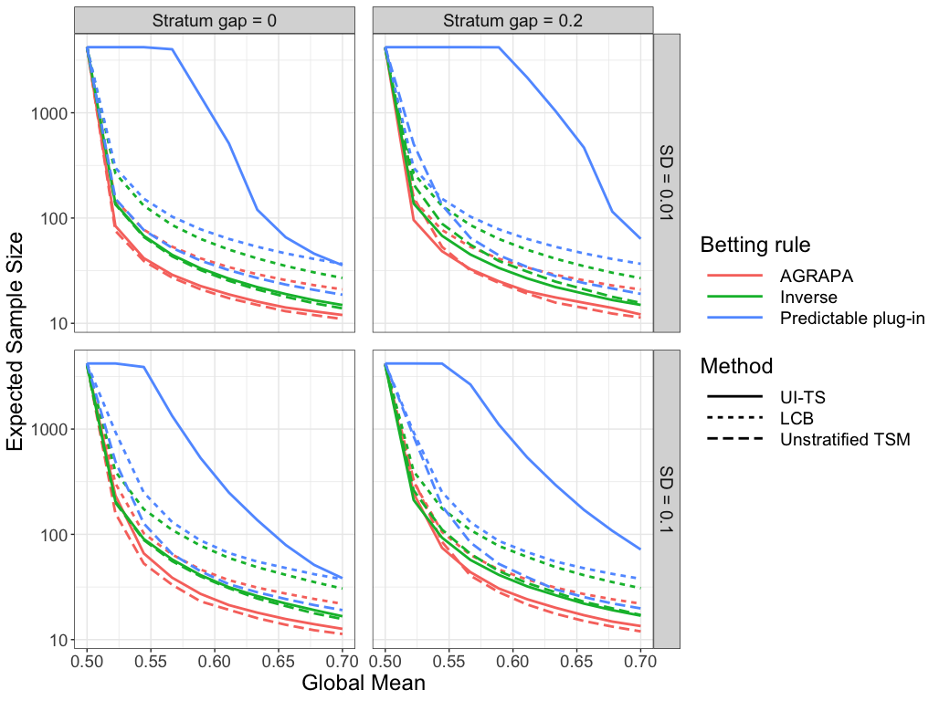
We simulated finite populations of size from truncated Gaussian superpopulations within each stratum. The true global mean ranged along a discrete grid from 0.5 to 0.7. Before truncation, the Gaussians had standard deviations with . The means were allowed to vary across strata according to a parameter that specified the distance between the strata so that . We truncated the Gaussians by redrawing samples that landed outside , which was rare since for all simulation settings the within-stratum means were bounded away from and was relatively small.
We implemented the same methods as the point-mass simulations (Section 7.1), and used the banding strategy with to compute the UI-TSs. For this simulation we also implemented a betting TSM drawing unstratified samples from the pooled population. That method served as a practical benchmark a statistician with control over the sampling design could use. In each simulation replicate, we drew a new finite population from the truncated Gaussian superpopulation, ran each method on the finite population, and recorded the sample size. If the method did not stop by the time the finite population had been consumed, we recorded a stopping time of 2100. We replicated the simulations 500 times and estimated the true expected stopping times of each method on each population by the (downward-biased) empirical mean.
The estimated expected stopping times are plotted in Figure 6. UI-TS with predictable plug-in bets and LCB (regardless of the betting strategy) had the largest estimated stopping times. The unstratified TSM generally had the lowest expected sample size (especially when used with AGRAPA bets), but the UI-TS had comparable performance when used with inverse or AGRAPA bets. When the stratum means differed, was small, and the alternative was close to the null, the UI-TS was slightly sharper than unstratified sampling. This is in keeping with the classical theory of stratification in terms of MSE: stratification improves efficiency when across-strata variation is large compared to within-stratum variation [Neyman, 1934, Cochran, 1977].
8 Conclusions
Stratified inference about population means arises in a large range of applied problems, including auditing, measurement, survey sampling, and randomized controlled trials. We constructed sequential nonparametric stratified tests that are practical and powerful in practice. The tests represent the global null as a union of intersection hypotheses; each intersection specifies the mean in every stratum. The tests construct an intersection test supermartingale (I-TSM) for each intersection hypothesis, then compute a -value for the global null as the reciprocal of the smallest of those I-TSMs, truncated above at 1: a union-intersection test sequence (UI-TS). Ville’s inequality guarantees that the chance the UI-TS ever exceeds is at most under the global null. UI-TSs require substantially smaller samples than the simple approach of combining simultaneous stratumwise lower confidence bounds (LCBs), but their computational cost is higher.
This approach provides the analyst considerable latitude to optimize the UI-TS: the I-TSM for each intersection null can use different tuning parameters and can interleave samples from different strata in different ways (“stratum selection”). In practice, when the tuning parameters are chosen appropriately, round-robin stratum selection performs well when strata are of equal size.
We extended the criterion of Kelly optimality to stratified sampling. Because it optimizes stopping time (the sample size for the hardest-to-reject intersection null) rather than the overall sample size required to reject every intersection null, the Kelly optimal UI-TS is not necessarily the most efficient when tests of different intersections can sample from the strata in different ways (i.e., use different stratum selection strategies). We navigated this issue by examining heuristic selection strategies that do not depend on the intersection null: round-robin or “greedy” UCB-style selection, targeting the growth of the smallest I-TSM in the union. Open-source Python software that implements these approaches and that generated the figures and tables herein are available at https://github.com/spertus/UI-NNSMs.
Future directions.
Finding (approximately) Kelly-optimal selections that minimize the expected sample size (rather than the expected stopping time) is an important open challenge for sequential stratified inference. We conjecture that when the selections do not depend on the intersection null, this problem is approximately solved by greedy strategies like the one we examined.
Another direction for research is to evaluate the performance of TSMs targeting regret rather than Kelly-optimality [Orabona and Jun, 2022] and leveraging optimal portfolio theory [Cover, 1991]. If the analyst posits a prior on the alternative, the method of mixtures can be used to construct the GRO -value for unstratified sampling [Grünwald et al., 2024]. The prior affects the efficiency (sample size) but not the frequentist validity of the test. Generalizing the method of mixtures to stratified inference may lead to efficient UI-TSs.
The UI-TSs we consider combine (independent) stratumwise -values by multiplication, which is optimal when every -value is larger than 1 [Vovk and Wang, 2021]. However, that condition can be difficult to ensure unless the stratumwise test supermartingales are allowed to depend on the intersection null. It may also be fruitful to consider combining functions other than the product. Other ways of testing the intersection hypothesis (e.g., combining -values by averaging or combining -values using Fisher’s combining function) may allow for consistent inference without much additional fuss [Spertus and Stark, 2022]. Indeed, Cho et al. [2024] show that average combining can lead to a test of power 1 and computationally tractable optimization over the union of intersection nulls.101010See [Ek et al., 2023] for an example of adaptively reweighted averaging of -values to test intersection hypotheses. However, in initial simulations comparing different combining functions, product combining tended to dominate averaging and Fisher combining unless the stratum-level TSMs were chosen very poorly.
Computing the UI-TS with product combining is a computational challenge. Partitioning the null into convex subsets allows I-TSMs to adapt to intersection nulls flexibly while keeping the minimization required to find the UI-TS tractable. This strategy could be made adaptive, refining the partition near the intersection nulls that are challenging to reject based on the data observed so far. It could also be generalized to more than two strata, but naive implementations may scale poorly. For another computational strategy, we constructed a class of convex UI-TSs that remain tractable to compute when there are many strata. An open problem is to maximize statistical efficiency for computationally tractable methods, for example by finding the nearest approximation to the Kelly optimal solution restricted to the class of all convex UI-TSs.
Acknowledgements
Jacob Spertus and Philip Stark’s work was supported by NSF grant 2228884. Mayuri Sridhar is grateful to the DoD NDSEG Fellowship program for their support while pursuing this work.
Appendix A Example: Kelly optimality and stratification
Consider using a UI-TS to test the composite null against a simple alternative for which, in each stratum, every value is the same: . That is, the population distribution is a point mass in each stratum. The UI-TS that achieves the minimum stopping time is the Kelly-optimal UI-TS, constructed by applying Lemma 2 and Lemma 3. Sampling is with replacement, so the Kelly-optimal rules do not depend on time.
To begin, take the betting rule
It is clearly Kelly-optimal when the within-stratum distributions are point masses: if , the bet is certain to succeed, and the rule bets the maximum permissible amount ; if , the bet cannot win, and the rule bets 0. Following Lemma 2, the Kelly-optimal selection rule always samples from a stratum with the largest expected log-growth. This gives an explicit formula for the Kelly-optimal I-TSM at :
where we have dropped the indicator because there is always at least one stratum with since the alternative is true. The Kelly-optimal UI-TS is thus:
Consider the special case , , and . Letting so , we can write
which is minimized when the two terms inside the parentheses are equal. That is, the minimizer satisfies
This nonlinear equation can be solved numerically for any . The stopping time is the value of at which crosses :
and the Kelly-optimal stopping time is . Now, it always holds that and, in this instance, since the maximum sampling depth in any one of the two strata is no more than the stopping time. Thus
and the Kelly-optimal stopping time bounds the Kelly-optimal sample size in this case.
A.1 Comparison to Kelly-optimal betting TSM
Consider the previous example but with unstratified sampling: each draw is equally likely to yield or . The expected log-growth of a betting TSM with bet is
| (7) |
When and are both bigger than 1/2, the gambler is guaranteed to make money, so the maximal bet is optimal. When or is less than 1/2 but , the optimal bet can be found by setting the derivative of the expected log-growth equal to zero and solving for , which yields
Let be the Kelly-optimal betting TSM, using as the bet. By Wald’s equation the expected stopping time and sample size of the level test using is
where the denominator is found by plugging into 7.
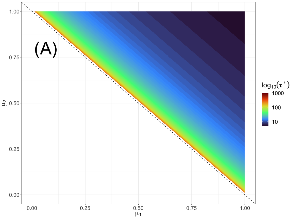
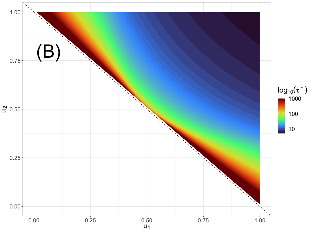
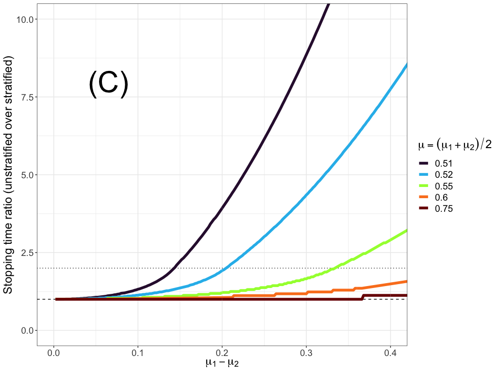
Figure 7 shows the expected stopping times of level tests based on (A) a Kelly-optimal betting UI-TS and (B) an unstratified Kelly-optimal betting TSM over a range of and in the alternative. Panel (C) plots the ratio of the betting TSM stopping time over the betting UI-TS stopping time, giving a sense of the gains to stratification. Using stratified sampling and a Kelly-optimal UI-TS is always superior to using unstratified sampling with a betting TSM in terms of stopping time. To translate to sample size, the UI-TS stopping times should be multiplied by 2. In terms of sample size, stratified sampling is beneficial when the margin is small and the gap between the strata is large.
Appendix B Proofs
B.1 Proof of Lemma 1
We restate Lemma 1 for reference:
Lemma.
For each stratum , define the sequence where
Then:
-
1.
are separately sequentially valid lower confidence bounds, in the sense that whenever :
-
2.
are simultaneously sequentially valid lower confidence bounds, in the sense that whenever :
Proof.
Part 1 of Lemma 1, on the separate validity of the lower confidence bounds (LCBs), follows immediately by inverting level tests constructed from within-stratum betting TSMs. Indeed, is the value of for which the within-stratum TSM equals : . The corresponding within-stratum -value is , which implies each is a LCB satisfying the first claim. See Waudby-Smith and Ramdas [2024].
Part 2 follows from the closed testing principle: recall that the family-wise error rate for a collection of partial hypotheses is controlled if is rejected only when every intersection of subsets of involving is rejected. Consider the partial hypotheses
At time , we reject if . If for , then
| (8) |
for any nonempty subset of . If are defined as in the lemma statement, at times we reject for all .
For example, suppose and . Then and . The 2-way intersection hypothesis corresponds to the test statistic
and is thus rejected along with the partial hypotheses. Extending this result to is obvious. Every intersection hypothesis will be rejected by the product of constituent TSMs, and by closed testing the LCBs are simultaneously below the true stratum-wise means with probability . The result also holds for average combining. ∎
B.2 Proof of Lemma 2
Proof.
The expected log-growth of I-TSM is
where the expectation is with respect to the sampling and the stratum selections. For any fixed selection strategy , the overall expected log-growth is an increasing function of the expected-log growth within strata, and is maximized when each is maximized. This is ensured by using the Kelly optimal bet within each stratum.
Now, choose the bets so that each term is maximized. The selection probabilities
maximize because they always draw from a stratum with the largest expected log growth. ∎
Appendix C Computation
Computing involves minimizing an expensive-to-compute function over . The difficulty of that optimization problem depends on the functional form of . In particular, finding the minimum over is hard when the bets and selections can depend arbitrarily on . Exhaustive search is possible when the exact boundary , defined in Section 4.2, is known and its cardinality is small. A partitioning strategy (like the banding strategy presented above) can be used when is small. Enumerating only the vertices of solves the problem when the bets and selections are -oblivious, and is practical for moderate . Finally, inverse bets make the problem convex and amenable to gradient descent strategies for optimization.
C.1 Brute-force search for discrete, finite populations
Let denote the possible values of elements of stratum . In general, and may be uncountably infinite. However, when is finite, the number of possible stratum means is also finite. If this holds for all , then is finite, and may be small enough to enumerate the set , enabling exhaustive minimization.
How large is ? The number of possible means is at most the number of possible distinguishable populations. The number of size- bags with elements in is:
This follows from Feller’s ‘stars and bars’ argument, partitioning the numbers into bins (all but one of which could be empty), each corresponding to a value in .
However, in many practical applications (e.g., stratified risk-limiting comparison audits), the size of is reduced because elements of have a relatively small least common multiple. For example, if then
and
In general,
for
where is the least common multiple of the numbers in the set . This implies that , a significant reduction in when the elements of are multiples of each other.
Now, the size of depends on the number of possible intersections of stratum-wise means lying near . An upper bound on is the number of possible within-stratum means:
This upper bound grows rapidly with , , and , but can be very loose.
An exact count of the number of means is possible in simple cases. For instance when the strata are of equal size () and binary (), the number of possible vectors of stratum means is:
This is large even for moderate when .
C.2 Vertex enumeration for -oblivious selections and bets
Suppose and are -oblivious. The minimum of is in , the vertices of the polytope . We establish this result by showing that is log-concave in .
The first two partial derivatives of are:
All the mixed partials are 0, while the second partials are all non-positive, and strictly negative if for some and all . Thus, the Hessian of is negative semi-definite, is concave in . Since is log-concave, it is quasi-concave: its value on any line segment within is not smaller than the smaller of its values at the ends of the segment. Since, only vertices of are not strict convex combinations of other points in , the minimum over is attained at a vertex of . may be substantially smaller than . If is small enough, we can compute by enumerating the values of for all .
C.2.1 The size of
We derive in an important special case: and . If is even then the elements of have elements equal to 1 and the rest equal to 0:
If is odd, an exemplar element of is a -vector with values equal to 1, exactly one value equal to , and the rest equal to 0. That is:
When the strata vary in size, there can be fewer or more vertices than this. The vertices can be enumerated, e.g., using the python package pypoman, which provides rapid enumeration for or so. As an example, when , , and , we must compute 51,480 I-TSMs each of length . As grows, the vertex enumeration approach eventually becomes infeasible.
C.3 Inverse bets
Inverse bets lead the set of I-TSMs to be log-convex in . To start simply, let . The log I-TSM is equal to:
which is convex since is convex and non-negative linear combinations of convex combinations are convex.
Now, to generalize, let for . Figure 8 plots this bet across , alongside other betting strategies. We have
The first partial derivative is
the mixed partials are all zero, and the second partials are given by the quotient rule:
where
Now, the denominator is always positive, and for each index the numerator is:
where the last inequality follows because and . Thus, the Hessian of is positive semidefinite when inverse bets are used, and the I-TSM is log-convex.
We also note that the bet leads to a log-convex I-TSM. (The proof is laborious but follows the same steps as above.) However, we found this bet does not yield a particularly efficient UI-TS. Higher efficiency can be achieved by generalizing to and setting to predictably adapt to the alternative. Unfortunately, the resulting I-TSM cannot be guaranteed to be log-convex except when and .

C.4 Inverse betting computation times
When inverse bets are used for every I-TSM, computing the UI-TS is a convex program with linear constraints. We computed the UI-TS using solvers.cp from version 1.3.2 of the cvxpy module.111111https://cvxopt.org/userguide/solvers.html, last visited 28 August 2024. To evaluate computation times, we constructed a range of stratified populations with and for all : the populations contained as many as 50 equal-sized strata with 100 units in each stratum. For each population, every unit in every stratum was equal to the global mean . We compared the time it took to compute the entire length- UI-TS (minimizing at every time ) and length- LCB sequence. We also examined the respective sample sizes when testing the global null at level . Both methods used inverse bets and round-robin selections.
Results appear in Table 2. LCB was always faster to run and its run time scaled sub-linearly in and . The UI-TS run time increased linearly in and faster in . The run time increases rapidly with because cvxopt is more computationally demanding as increases and because the number of optimization problems increases with the length of the interleaving. The computation time of the UI-TS could be reduced by limiting the number of optimizations, e.g., by computing the minimum only occasionally (say, every 50 samples) or just by ceasing computation once the UI-TS crosses (i.e., at the stopping time). The UI-TS had substantially smaller sample sizes than LCB, especially for large : the penalty for stratification is much less for UI-TS than for LCB.
| Run time (s) | Sample size () | |||||
| LCB | UI-TS | LCB | UI-TS | |||
| 10 | 2 | 20 | 1.0 | 4.5 | – | – |
| 3 | 30 | 1.3 | 2.4 | – | – | |
| 5 | 50 | 2.2 | 7.0 | – | – | |
| 10 | 100 | 4.5 | 29.3 | – | – | |
| 50 | 500 | 22.5 | 744.3 | – | – | |
| 100 | 2 | 200 | 4.9 | 69.0 | 55 | 29 |
| 3 | 300 | 7.3 | 158.2 | 83 | 30 | |
| 5 | 500 | 12.1 | 448.7 | 137 | 32 | |
| 10 | 1,000 | 32.7 | 2067.4 | 274 | 38 | |
| 50 | 5,000 | 164.3 | 50,938.9 | 1,367 | 77 | |
Appendix D Stratified sequential testing for a simple null
Suppose we wish to test a simple null against a simple alternative . While we were generally interested in the composite null in this paper, a simple null provides a simple optimal strategy: the SPRT of Wald [1945].
Specifically, let be the null population in stratum . Analogously, is the within-stratum alternative. Furthermore, let denote the probability density at under uniform sampling with or without replacement from . Following the construction of the SPRT within each stratum, form the terms
The running product measures evidence against the simple null within stratum , and the product across strata:
is a martingale when is true. Furthermore, Wald [1945] shows that this choice of maximizes , i.e., it is Kelly-optimal. The growth rate optimality of the SPRT is analogous to the power optimality of the likelihood ratio in the fixed-sample case, as in the canonical lemma of Neyman and Pearson [1933].
If the null is simple and the alternative is composite, the SPRT is still valid with denominator . However, there is no uniquely optimal choice for the numerator. One option is to form predictable estimates of the parameters of and plug them into the numerator [Ramdas et al., 2023]. The method of mixtures leads to a consistent test, and is GRO (in the terminology of Grünwald et al. [2024]) when the mixing distribution is a generative prior, from which the alternative was drawn.
References
- Anderson [1967] T.W. Anderson. Confidence limits for the expected value of an arbitrary bounded random variable with a continuous distribution function. Bulletin of the International Statistical Institute, 43:249–251, 1967.
- Appel and Stark [2020] A.W. Appel and P.B. Stark. Evidence-based elections: Create a meaningful paper trail, then audit. Georgetown Law Technology Review, 4.2:523–541, 2020. https://georgetownlawtechreview.org/wp-content/uploads/2020/07/4.2-p523-541-Appel-Stark.pdf.
- Auer et al. [2002] P. Auer, N. Cesa-Bianchi, and P. Fischer. Finite-time analysis of the multiarmed bandit problem. Mach. Learn., 47(2–3):235–256, may 2002. ISSN 0885-6125. doi: 10.1023/A:1013689704352. URL https://doi.org/10.1023/A:1013689704352.
- Bahadur and Savage [1956] R.R. Bahadur and L.J. Savage. The nonexistence of certain statistical procedures in nonparametric problems. The Annals of Mathematical Statistics, 27(4):1115 – 1122, 1956. doi: 10.1214/aoms/1177728077. URL https://doi.org/10.1214/aoms/1177728077.
- Berger and Boos [1994] Roger L. Berger and Dennis D. Boos. P values maximized over a confidence set for the nuisance parameter. Journal of the American Statistical Association, 89(427):1012–1016, 1994. ISSN 01621459. URL http://www.jstor.org/stable/2290928.
- Berry and Fristedt [1985] D.A. Berry and B. Fristedt. Bandit problems: Sequential allocation of experiments. Springer, October 1985. ISBN 0412248107.
- Bickel [1992] P.J. Bickel. Inference and auditing: The Stringer bound. International Statistical Review, 60(2):197–209, 1992. ISSN 0306-7734. doi: 10.2307/1403650. URL https://www.jstor.org/stable/1403650.
- Bittinger et al. [2022] S. Bittinger, M. Yates, and M. Phillips. Statistical sampling and extrapolation: Due process challenges in the false claims act litigation and medicare appeals arenas, 2022. URL https://www.americanbar.org/groups/health_law/publications/health_lawyer_home/december-2022/statistical-sampling-and-extrapolation/.
- Cho et al. [2024] B. Cho, K. Gan, and N. Kallus. Peeking with PEAK: sequential, nonparametric composite hypothesis tests for means of multiple data streams, 2024. URL http://arxiv.org/abs/2402.06122.
- Cochran [1977] W.G. Cochran. Sampling Techniques. John Wiley & Sons, Inc., New York, 3rd edition, 1977.
- Cournot [1843] A.A. Cournot. Exposition of the Theory of Chances and Probabilities. NG Verlag, 1843. URL https://arxiv.org/pdf/1902.02781. Translated by Oscar Sheynin (2013).
- Cover [1991] T.M. Cover. Universal portfolios. Mathematical Finance, 1:1–29, 1991.
- Ek et al. [2023] A. Ek, P.B. Stark, P.J. Stuckey, and D. Vukcevic. Adaptively weighted audits of instant-runoff voting elections: AWAIRE. In M. Volkamer, D. Duenas-Cid, P. Rønne, P.Y.A. Ryan, J. Budurushi, O. Kulyk, A. Rodriguez Pérez, and I. Spycher-Krivonosova, editors, Electronic Voting, pages 35–51, Cham, 2023. Springer Nature Switzerland. ISBN 978-3-031-43756-4.
- Fienberg and Tanur [1996] S.E. Fienberg and J.M. Tanur. Reconsidering the fundamental contributions of Fisher and Neyman on experimentation and sampling. International Statistical Review, 64(3):237–253, 1996. ISSN 0306-7734. URL https://www.jstor.org/stable/1403784.
- Fienberg et al. [1977] S.E. Fienberg, J. Neter, and R.A. Leitch. Estimating total overstatement error in accounting populations. Journal of the American Statistical Association, 72:295–302, 1977.
- Gaffke [2005] N. Gaffke. Three test statistics for a nonparametric one-sided hypothesis on the mean of a nonnegative variable. Mathematical Methods of Statistics, 14:451–467, 2005.
- Grünwald et al. [2024] P. Grünwald, R. de Heide, and W. Koolen. Safe Testing. Journal of the Royal Statistical Society Series B: Statistical Methodology, March 2024. ISSN 1369-7412. doi: 10.1093/jrsssb/qkae011. URL https://doi.org/10.1093/jrsssb/qkae011.
- Hansen et al. [1953] M.H. Hansen, W.N. Hurwitz, and W.G. Madow. Sample survey methods and theory, volume 1: method and applications. Wiley, 1953.
- Hoeffding [1963] W. Hoeffding. Probability inequalities for sums of bounded random variables. Journal of the American Statistical Association, 58:13–30, 1963.
- Howard et al. [2019] L. Howard, R.L. Rivest, and P.B. Stark. A review of robust post-election audits: Various methods of risk-limiting audits and Bayesian audits. Technical report, Brennan Center for Justice, 2019. https://www.brennancenter.org/sites/default/files/2019-11/2019_011_RLA_Analysis_FINAL_0.pdf.
- Howard et al. [2021] S.R. Howard, A. Ramdas, J. McAuliffe, and J. Sekhon. Time-uniform, nonparametric, nonasymptotic confidence sequences. The Annals of Statistics, 49(2), 2021. URL https://doi.org/10.1214%2F20-aos1991.
- Kaplan [1987] H.M. Kaplan. A method of one-sided nonparametric inference for the mean of a nonnegative population. The American Statistician, 41:157–158, 1987.
- Kish [1965] L. Kish. Survey Sampling. John Wiley & Sons, Inc., New York, 1965.
- Lai and Robbins [1985] T.L Lai and Herbert Robbins. Asymptotically efficient adaptive allocation rules. Advances in Applied Mathematics, 6(1):4–22, 1985. ISSN 0196-8858. doi: https://doi.org/10.1016/0196-8858(85)90002-8. URL https://www.sciencedirect.com/science/article/pii/0196885885900028.
- Learned-Miller and Thomas [2020] E. Learned-Miller and P.S. Thomas. A new confidence interval for the mean of a bounded random variable. 2020. URL https://arxiv.org/abs/1905.06208.
- Lehmann [1993] E. L. Lehmann. The Fisher, Neyman-Pearson theories of testing hypotheses: One theory or two? Journal of the American Statistical Association, 88(424):1242–1249, 1993. ISSN 01621459. URL http://www.jstor.org/stable/2291263.
- Lehmann and Romano [2005] E.L Lehmann and J.P. Romano. Testing Statistical Hypotheses. Springer, New York, 3rd edition, 2005.
- Marcus et al. [1976] R. Marcus, E. Peritz, and K. R. Gabriel. On closed testing procedures with special reference to ordered analysis of variance. Biometrika, 63(3):655–660, 1976. ISSN 00063444. URL http://www.jstor.org/stable/2335748.
- Maurer and Pontil [2009] A. Maurer and M. Pontil. Empirical bernstein bounds and sample variance penalization. 2009. URL https://arxiv.org/abs/0907.3740.
- Neyman [1934] J. Neyman. On the two different aspects of the representative method: The method of stratified sampling and the method of purposive selection. Journal of the Royal Statistical Society, 97(4):558–625, 1934. URL https://www.jstor.org/stable/2342192.
- Neyman and Pearson [1933] J. Neyman and E.S. Pearson. On the problem of the most efficient tests of statistical hypotheses. Philosophical Transactions of the Royal Society of London. Series A, 231:289–337, 1933. URL http://www.jstor.org/stable/91247.
- Orabona and Jun [2022] F. Orabona and K.-S. Jun. Tight concentrations and confidence sequences from the regret of universal portfolio, 2022. URL https://arxiv.org/abs/2110.14099.
- Ottoboni et al. [2018] K. Ottoboni, P.B. Stark, M. Lindeman, and N. McBurnett. Risk-limiting audits by stratified union-intersection tests of elections (SUITE). In Electronic Voting. E-Vote-ID 2018. Lecture Notes in Computer Science. Springer, 2018. https://link.springer.com/chapter/10.1007/978-3-030-00419-4_12.
- Panel on Nonstandard Mixtures of Distributions [1988] Panel on Nonstandard Mixtures of Distributions. Statistical Models and Analysis in Auditing: A Study of Statistical Models and Methods for Analyzing Nonstandard Mixtures of Distributions in Auditing. National Academy Press, Washington, D.C., 1988.
- Ramdas et al. [2023] A. Ramdas, P. Grünwald, V. Vovk, and G. Shafer. Game-theoretic statistics and safe anytime-valid inference. Statistical Science, 38(4):576 – 601, 2023. doi: 10.1214/23-STS894. URL https://doi.org/10.1214/23-STS894.
- Robbins [1952] H. Robbins. Some aspects of the sequential design of experiments. Bulletin of the American Mathematical Society, 58:527–535, 1952.
- Robbins and Siegmund [1974] H. Robbins and D. Siegmund. The Expected Sample Size of Some Tests of Power One. The Annals of Statistics, 2(3):415 – 436, 1974. doi: 10.1214/aos/1176342704. URL https://doi.org/10.1214/aos/1176342704.
- Romano and Wolf [2000] J.P. Romano and M. Wolf. Finite sample nonparametric inference and large sample efficiency. The Annals of Statistics, 28(3):756 – 778, 2000. doi: 10.1214/aos/1015951997. URL https://doi.org/10.1214/aos/1015951997.
- Savage [1951] L.J. Savage. The theory of statistical decision. Journal of the American Statistical Association, 46(253):55–67, 1951. ISSN 01621459. URL http://www.jstor.org/stable/2280094.
- Shafer [2021] G. Shafer. Testing by betting: A strategy for statistical and scientific communication. Journal of the Royal Statistical Society: Series A (Statistics in Society), 184:407–431, 04 2021. doi: 10.1111/rssa.12647.
- Shafer and Vovk [2019] G. Shafer and V. Vovk. Game Theoretic Foundations for Probability and Finance. Wiley Series in Probability and Statistics, 2019.
- Shafer et al. [2011] G. Shafer, A. Shen, N. Vereshchagin, and V. Vovk. Test martingales, Bayes factors and p-values. Statistical Science, 26(1):84–101, February 2011. ISSN 0883-4237, 2168-8745. doi: 10.1214/10-STS347. URL https://projecteuclid.org/journals/statistical-science/volume-26/issue-1/Test-Martingales-Bayes-Factors-and-p-Values/10.1214/10-STS347.full.
- Silvapulle [1996] M.J. Silvapulle. A test in the presence of nuisance parameters. Journal of the American Statistical Association, 91(436):1690–1693, 1996. doi: 10.1080/01621459.1996.10476739.
- Spertus and Stark [2022] J.V. Spertus and P.B. Stark. Sweeter than SUITE: Supermartingale stratified union-intersection tests of elections. In Robert Krimmer, Melanie Volkamer, David Duenas-Cid, Peter Rønne, and Micha Germann, editors, Electronic Voting, pages 106–121, Cham, 2022. Springer International Publishing. ISBN 978-3-031-15911-4.
- Stanley et al. [2023] P. Stanley, J.V. Spertus, J. Chiartas, P.B. Stark, and T. Bowles. Valid inferences about soil carbon in heterogeneous landscapes. Geoderma, 430:116323, February 2023. ISSN 0016-7061. doi: 10.1016/j.geoderma.2022.116323. URL https://www.sciencedirect.com/science/article/pii/S0016706122006309.
- Stark [2020] P.B. Stark. Sets of half-average nulls generate risk-limiting audits: SHANGRLA. Financial Cryptography and Data Security, Lecture Notes in Computer Science, 12063, 2020. Preprint: http://arxiv.org/abs/1911.10035.
- Stark [2023] P.B. Stark. ALPHA: Audit that learns from previously hand-audited ballots. The Annals of Applied Statistics, 17(1):641 – 679, 2023. doi: 10.1214/22-AOAS1646. URL https://doi.org/10.1214/22-AOAS1646.
- Stark [2008] Philip B. Stark. Conservative statistical post-election audits. The Annals of Applied Statistics, 2(2):550 – 581, 2008. doi: 10.1214/08-AOAS161. URL https://doi.org/10.1214/08-AOAS161.
- Tchouproff [1923] Al. A. Tchouproff. On the mathematical expectation of the moments of frequency distributions in the case of correlated observations (chapter i-iii). Metron, 2:461–493, 1923.
- Thompson [1933] W.R. Thompson. On the likelihood that one unknown probability exceeds another in view of the evidence of two samples. Biometrika, 25(3-4):285–294, 12 1933. ISSN 0006-3444. doi: 10.1093/biomet/25.3-4.285. URL https://doi.org/10.1093/biomet/25.3-4.285.
- Tsui and Weerahandi [1989] K.-W. Tsui and S. Weerahandi. Generalized p-values in significance testing of hypotheses in the presence of nuisance parameters. Journal of the American Statistical Association, 84(406):602–607, 1989. ISSN 01621459. URL http://www.jstor.org/stable/2289949.
- US CMS [2023] US CMS. Medicare program integrity manual, 2023. URL https://www.cms.gov/regulations-and-guidance/guidance/manuals/downloads/pim83c08.pdf.
- US DHS [2020] US DHS. Medicare contractors were not consistent in how they reviewed extrapolated overpayments in the provider appeals process, 2020. URL https://oig.hhs.gov/oas/reports/region5/51800024.pdf.
- Ville [1939] J. Ville. Étude critique de la notion de collectif. 1939. URL http://eudml.org/doc/192893.
- Vovk and Wang [2021] V. Vovk and R. Wang. E-values: Calibration, combination and applications. The Annals of Statistics, 49(3), June 2021. doi: 10.1214/20-aos2020. URL https://doi.org/10.1214%2F20-aos2020.
- Wald [1944] A. Wald. On cumulative sums of random variables. The Annals of Mathematical Statistics, 15(3):283 – 296, 1944. doi: 10.1214/aoms/1177731235. URL https://doi.org/10.1214/aoms/1177731235.
- Wald [1945] A. Wald. Sequential tests of statistical hypotheses. The Annals of Mathematical Statistics, 16:117–186, 1945.
- Wald [1947] A. Wald. Sequential Analysis. Dover Publications, New York, 1947.
- Wald [1950] A. Wald. Statistical Decision Functions. John Wiley and Sons, New York, 1950.
- Wasserman [2004] L. Wasserman. All of Statistics. Springer, 2004.
- Waudby-Smith and Ramdas [2024] I. Waudby-Smith and A. Ramdas. Estimating means of bounded random variables by betting. Journal of the Royal Statistical Society Series B: Statistical Methodology, 86, 2024. URL https://academic.oup.com/jrsssb/article/86/1/1/7043257.
- Wendell and Schmee [1996] J.P. Wendell and J. Schmee. Exact inference for proportions from a stratified finite population. Journal of the American Statistical Association, 91:825–830, 1996.
- Wright [1991] T. Wright. Exact Confidence Bounds when Sampling from Small Finite Universes. Springer-Verlag, New York, 1991.