Predictions for photon-jet correlations at forward rapidities in heavy-ion collisions

Abstract

In this work, we study for the first time jet-medium interactions in heavy-ion collisions with introduction of saturation and Sudakov effects with parameters tuned for upcoming forward calorimeter acceptances in experiments, in particular the ALICE FoCal detector. We focus on $\gamma+$jet correlations by taking into account in-medium parton evolution using the BDIM equation that describes jet interactions with the quark-gluon plasma (QGP) combined with vacuum-like emissions (VLE). We systematically introduce the early time gluon saturation dynamics through the small-$x$ Improved Transverse Momentum Dependent factorization (ITMD). For our purpose, we use Monte Carlo programs KATIE and TMDICE to generate hard events and in-medium parton evolution, respectively. We present results of azimuthal correlations and nuclear modification ratios to gauge the impact of the gluon saturation effects at early time for the in-medium jet energy loss.

[a]Institute of Nuclear Physics, Polish Academy of Sciences, ul. Radzikowskiego 152, 31-342 Krakow, Poland [b]Institute of Physics of the Czech Academy of Sciences, Na Slovance 1999, 18221 Prague 8, Czech Republic [c]Faculty of Physics, Astronomy and Applied Computer Science and Mark Kac Center for Complex Systems Research, Jagiellonian University, ul. Lojasiewicza 11, 30-348 Krakow, Poland [d]Faculty of Material Engineering and Physics, Cracow University of Technology, ul. Podchorazych 1, 30-084 Krakow, Poland [e]Department of Physics and Technology, University of Bergen, 5007 Bergen, Norway

1 Introduction

Quantum Chromodynamics (QCD) is a well established theory of strong interactions. However, it predicts phenomena that still need experimental confirmation. One such a puzzle is the phenomenon of “gluon saturation” [1], where the growth of gluon density slows down due to a balance between gluon splittings and recombinations. The theoretical formalism that is developed to tackle saturation is the Color Glass Condensate (CGC) effective theory (as reviewed in [2, 3]). Saturation is a QCD prediction anticipated at high-energy hadron collisions. While multiple experimental indications suggest its presence – exemplified by direct data [4, 5, 6] as well as saturation-based approaches correlated with the HERA, RHIC and LHC data [7, 8, 9, 10, 11, 12, 13, 10, 14].

The LHC program offers significant potential for uncovering evidence of the gluon saturation. However, currently, no LHC experiments explicitly aim to study saturation physics, most likely to be observed in processes where longitudinal momentum of a target is probed at values $x<10^{-5}$. In the LHC kinematics for jets this corresponds to particle production in a forward rapidity region. The forthcoming FoCal calorimeter of the ALICE collaboration will bridge this gap [15, 16]. Designed to achieve high-resolution measurements of jets and photons in the forward region, it will cover pseudorapidities within the range $3.4<\eta<5.8$. These possible measurements have caught a lot of attention and motivated many predictions which are optimistic for saturation to be found in $p$A collisions as they offer nuclear density enhancement in favor of saturation as compared $pp$ collisions [17, 18, 19, 12, 20, 21, 22, 23, 24] (see also [25] for review).

An intriguing possibility for investigating saturation is to study forward jet production in AA collisions. This system, similarly to $p$A collisions, offers enhancement of nuclear density. The process is, however, more complex, as scattering events of heavy-ions involving large momentum transfer result in creation of highly energetic jets immersed in a medium. These jets serve as “probes” for examining the properties of the densely interacting medium formed during high-energy heavy-ion collisions [26, 27]. The basic goal of the paper is to investigate to what extend the saturation effects are visible in final states of heavy-ion collisions. Naively, one could think that the saturation effects will be lost in the medium because the quark-gluon plasma (QGP) medium strongly modifies the properties of jets. However, the point is that the Forward Calorimeter (FoCal) of the ALICE experiment offers a possibility to look specifically in the forward rapidity region, that allows to probe parton densities at a very low $x$ region, where in $p$Pb collisions the saturation effects were shown to be large and where back-to-back configurations are suppressed [18, 28, 22]. In addition, both the ATLAS and the CMS detectors will, in the future, also feature a Forward Calorimeter (FCal) and a Hadronic Forward (HF) calorimeter with the pseudorapidity ranges of $3.1<\eta<4.9$ and $3.0<\eta<5.2$, respectively [29, 30], crucial for capturing and studying forward-scattering events. We therefore expect that the suppression of particle production in the forward acceptance region of the detector will be large enough to be visible in PbPb collisions.

The production of high-energy particles, like partons or photons, in “hard” processes occurs over very short time intervals, with $\tau\sim 1/p_{\scriptscriptstyle T}\lesssim 0.1$ fm/c. Consequently, their features can potentially be altered by interactions in the final state while they traverse the medium. The cross-sections for energetic particle production can be calculated using perturbative QCD methods, making them valuable ‘tomographic’ tools for probing the properties of the created medium [31, 32, 33, 34, 35, 36, 37, 38, 39].

In collisions involving Pb nuclei at the LHC, the impact of the produced medium has been investigated at mid-rapidity by studying pairs of back-to-back dijets. These dijets displayed significant imbalance in their transverse momenta [40, 41]. However, the advantage of having a large yield of dijets compared to pairs of $\gamma$+jet is counterbalanced by the loss of information about the initial characteristics of the probes, specifically prior to their interactions with the medium. Additionally, correlating two probes that both undergo energy loss introduces a bias toward scatterings happening at the medium surface and aligned tangentially to it. At the leading order (LO) in the QCD coupling constant, photons ($\gamma$) are generated in tandem with a closely associated quark (jet) having the same transverse momentum. Furthermore, these photons interact only weakly with the medium. The yield of isolated photons in PbPb collisions was found to align with expectations based on $pp$ data and the number of nucleon–nucleon collisions, with a nuclear modification factor $R_{AA}=0.99\pm 0.31\;\text{(stat.)}\pm 0.26\;\text{(syst.)}$. As a result, the production of $\gamma$-jet combinations has been identified as the optimal means for investigating the energy loss of partons within the medium [42, 43], recently through parametric modeling approach in central rapidities [44]. However, all these studies were performed in the central rapidity regions where the impact of the gluon saturation physics is expected to be small. In experimental contexts, events with an increased yield of prompt photons are selected using an isolation requirement. This requirement dictates that additional energy within a fixed-radius cone around the reconstructed photon direction must fall below a specified threshold. Consequently, “isolated photons” are primarily composed of prompt photons generated directly during the initial hard scattering. This isolation condition is used to suppress background photons originating from decays of neutral mesons, such as $\pi_{0}$, $\eta$ and $\omega$, which are predominantly created through jet fragmentation.

The paper is organized as follows. Section 2 introduces the gluon saturation physics as the initial conditions in the hard processes of the $\gamma$-jet formation. Next, in Section 3, we describe the energy loss mechanism of the jet inside the medium undergoing quenching due to vacuum-like emissions as well as coherent energy loss and multiple scatterings within the medium. In Section 4, we present the results for the magnitude of the jet quenching in the forward rapidity region based on anticipated parameters of the FoCal detector. Additionally, we present quantitative comparisons between different configurations of the saturation and medium-jet suppression effects for rapidity and azimuthal angular distributions. Finally, in Section 5, we summarize our findings and present conclusions. In Appendix A, we discuss some uncertainties of our analyses, and in Appendix B, we describe our Monte Carlo algorithm used for generation of vacuum-like emissions (VLE).

2 Pre-medium scenario

As mentioned in the previous section, the process we consider here, depicted schematically in Fig. 1, involves $\gamma+$jet final states being produced in the forward direction in high-energy heavy-ion collisions:

$$A_{1}+A_{2}\rightarrow\gamma+\mathrm{jet}+X\,,$$ (1)

where $A_{1},A_{2}$ denote two colliding ions (e.g. of Pb) and $X$ is an unmeasured final state. The effective theory that allows to calculate the final states in this scenario is CGC, as already mentioned in Introduction. It can be further shown that it leads to the so-called Improved Transverse Momentum Dependent Factorization (ITMD) [45, 46] which is formulated in the momentum space. The later framework is expressed as gauge-invariant transverse-momentum-dependent (TMD) parton density functions convoluted with a gauge-invariant hard matrix element. For a generic process, this framework represents a limit of CGC neglecting genuine twists, i.e. contributions where $Q_{s}\!<\!p_{T}$. This is a good approximation when considering jet physics. For the process that we consider the relation is exact, i.e. ITMD is equivalent to CGC [47, 48].

The leading pre-quenching partonic process is

$$q(k_{1})+g^{*}(k_{2})\rightarrow q(p_{1})+\gamma(p_{2})\,,$$ (2)

where $q$ denotes on-shell quarks while $g^{*}$ – a space-like gluon. In the configuration where the final state is such that the observed jet and photon are both in the forward direction, the longitudinal momenta of the incoming partons are strongly ordered [17, 18, 49, 28]:

$$k_{1}=x_{1}\,P_{1}, k_{2}=x_{2}\,P_{2}+k_{2T}\,,$$ (3)

with $x_{1}\gg x_{2}$.

The cross section for the pre-quenching process is a direct extension of a cross-section formula for $pp$ and $p$A collisions, and it reads [49, 28]

$$\frac{d\sigma^{AA\rightarrow\gamma+\mathrm{jet}+X}}{dy_{1}dy_{2}dp_{1T}dp_{2T}d\Delta\phi} =\frac{p_{1T}p_{2T}}{8\pi^{2}(x_{1}x_{2}s)^{2}}\sum_{a}x_{1}f_{a/A}(x_{1},\mu_{F}^{2})\,$$

$$\times|{\cal M}_{ag^{*}\to\gamma a}^{\mathrm{off-shell}}|^{2}{\cal F}(x_{2},k_{2T}^{2},\mu_{F}^{2})\,,$$ (4)

where ${\cal M}^{\mathrm{off-shell}}_{ag^{*}\to\gamma a}$ is the matrix element with one off-shell and one on-shell parton in the hard sub-process, $f_{a/A}(x_{1},\mu^{2})$ is the collinear quark-density distribution for the lead nucleus and ${\cal F}(x_{i},k_{iT}^{2},\mu_{F}^{2})$ is the operator-defined dipole gluon density obeying the nonlinear Balitsky–Kovchegov equation [50, 51]. The nonlinearity of the equation allows for recombination of gluons, which in the end leads to emergence of a saturation scale. The dipole gluon density, besides its dependence on $x$ and $k_{T}$, in general also depends on the hard scale introduced via the Sudakov form factor [52, 53, 54].

3 Medium scenario

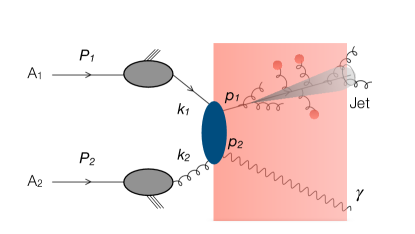
Figure 1: Quark-jet and prompt photon production via scattering of quark and gluon in hard nuclear collisions: colliding nuclei (horizontal ellipse) with the momenta $P_{1}$ and $P_{2}$ yield incoming quark and gluon (with the momenta $k_{1}$ and $k_{2}$) which interact in a hard scattering process (vertical ellipse) and yield a quark and a photon (with the momenta $q_{1}$ and $q_{2}$) which propagate through QGP indicated by the pink rectangle. The quark emits partons via vacuum-like shower (indicated by the blue line), and in the next stage in-medium scattering takes place (gluons attached to red bullets). Simultaneous fragmentation into a jet is denoted by the gray cone.

The evolution of parton jets produced in heavy-ion collisions undergoes further emissions, see Fig. 1, based on characteristic timescales of the processes.

1. At the beginning of jet evolution the color degrees of freedom of individual jet particles may not be resolved by the particles within a QGP medium. However, parton radiation in the vacuum, known as the vacuum-like emissions (VLE), is still possible [55]. Therefore, the evolution via such a parton emission follows the Dokshitzer–-Gribov–-Lipatov-–Altarelli–-Parisi (DGLAP) evolution equations [57, 58, 59]. Phase-space boundaries at which the colors of individual jet particles are resolved by the medium are described in Subsection 3.1.

2. As the medium particles resolve the colors of the individual jet particles, the latter undergo processes of scattering off the former as well as the medium-induced radiation. Here, we implement the evolution that follows the equations by Blaizot–Dominguez–Iancu–Mehtar-Tani (BDIM) [60, 61, 62]. We refer to this stage of the process as the BDIM evolution and discuss it in more detail in Subsection 3.2.

3.1 Vacuum-like emissions

In a vacuum, the high-energy partons produced as a result of the hard QCD collision undergo a reduction in their large virtuality down to the hadronization scale through successive splittings. These processes have been studied in detail theoretically [63, 64, 65] and implemented within Monte Carlo (MC) parton shower generators through the DGLAP evolution equations. It has been firmly established that there is a significant phase space for VLE occurring before any medium-induced modifications can develop [55, 66, 67, 68]. This vacuum-like phase space significantly impacts the amount of jet-energy loss based on the vacuum-set scales governing jet activity, such as multiplicity. Therefore, understanding this phase space is crucial for explaining numerous jet-quenching observables, such as the relative suppression between jets and hadrons [66, 69, 70, 71]. In light of these recent developments, we consider the possibility that a particle created in a hard initial collision can radiate partons as in the vacuum before entering a QGP-medium. Therefore, we presume that the initial parton $i$ undergoes parton branchings according to probability densities for emitting a particle $j$ given as

$$\frac{{\rm d}^{2}\mathcal{P}_{ji}}{{\rm d}Q^{2}{\rm d}z}=\frac{\alpha_{s}}{2\pi}\frac{1}{Q^{2}}P_{ji}(z)\,,$$ (5)

where $Q$ is the virtuality of the branching particle, $z$ is the energy fraction of the emitted particle and the functions $P_{ji}(z)$ are the DGLAP splitting functions at LO in QCD, given as

$$P_{qq}(z) =C_{F}\frac{1+z^{2}}{1-z}\,,$$ (6)

$$P_{gq}(z) =P_{qq}(1-z)\,,$$ (7)

$$P_{qg}(z) =T_{R}\left[z^{2}+(1-z)^{2}\right]\,,$$ (8)

$$P_{gg}(z) =C_{A}\left[\frac{1-z}{z}+\frac{z}{1-z}+z(1-z)\right]\,.$$ (9)

As shown in [55, 56], after entering the QGP medium, the individual color degrees of freedom of two jet-particles $i$ and $j$ may not be resolved by the medium for a certain decoherence time ($t_{\rm decoh}$) that can be estimated as [72, 73]

$$t_{\rm decoh}\approx\left(\frac{12}{\hat{q}\theta_{ij}^{2}}\right)^{1/3}\,,$$ (10)

where $\theta_{ij}$ is the branching angle for which a small angle approximation

$$\theta_{ij}\approx Q_{i}/\sqrt{E_{i}^{2}z(1-z)}\,,$$ (11)

was used. The average transverse momentum transfer $\hat{q}$ is defined via the changes over time $t$ of a particle traveling through the medium with the momentum component $k_{\perp}$ transverse to its original incident direction as

$$\hat{q}=\frac{{\rm d}\langle k_{\perp}^{2}\rangle}{{\rm d}t}\,.$$ (12)

On the other hand, a branching time of a radiating jet-particle $i$ due to the formation of bremsstrahlung can be estimated as

$$t_{\rm br}\approx 2E_{i}/Q_{i}^{2}\,.$$ (13)

Thus, one can estimate [55, 73, 74, 56] that as long as a pair of jet partons fulfills the condition

$$t_{\rm br}<t_{\rm decoh}\,,$$ (14)

parton branchings due to bremsstrahlung as in the vacuum occur faster than interactions with medium particles. Therefore, we consider emissions following Eq. (5) for jet particles in the QGP medium as long as Eq. (14) is not violated. Afterwards, both scatterings off medium particles as well as coherent medium-induced radiations that follow the well-known spectrum found by Baier, Dokshitzer, Mueller, Peigné and Schiff, and independently by Zakharow (BDMPS-Z) [75, 76, 77, 78, 79, 36, 80] occur. It is to be noted that an additional constraint for VLEs is given by

$$t_{\rm decoh}<t_{\rm L},$$ (15)

where $t_{\rm L}$ is the time at which the jet particles leave the medium. This constraint implements the requirement that the splitting is resolved within a finite distance inside the medium. This is equivalent to requiring that the splitting has an angle greater than a critical angle $\theta_{ij}>\theta_{c}$, where $\theta_{c}=\sqrt{12/(\hat{q}L^{3})}$. Using the double logarithmic approximation (DLA), where the multiplicity of gluons is dominated by the soft and collinear divergences in QCD, i.e. ${\rm d}N_{\text{\tiny DLA}}=\bar{\alpha}({\rm d}z/z)({\rm d}\theta/\theta)$ with $\bar{\alpha}=\alpha_{s}C_{i}/\pi$, the number of emitted gluons inside the medium can be estimated as [66]

$$N_{\text{\tiny DLA}}^{\text{in}}=2\bar{\alpha}\log\frac{R}{\theta_{c}}\left(\log\frac{E}{\omega_{c}}+\frac{2}{3}\log\frac{R}{\theta_{c}}\right)\,,$$ (16)

where $R$ is the jet-cone size and $\omega_{c}=\hat{q}L^{2}/2$ is the medium energy scale from multiple scattering.

It is important to distinguish here the longitudinal energies $E$ and $\omega$ of the leading and sub-leading jet particles, respectively, and the transverse momentum $p_{\scriptscriptstyle T}$ as measured in the detector. When measured at mid-rapidity, the jets are propagating perpendicularly to the beam axis and we can identify $E=p_{\scriptscriptstyle T}$. At forward rapidities, $\eta>1$, a very rough estimate gives $E\sim p_{\scriptscriptstyle T}{\rm e}^{\eta}$. Comparing to Eq. (16), we see that every unit of rapidity contributes for $E>\omega_{c}$, that is with an additional gluon emitted deep inside the QGP. Studying jets at forward rapidities therefore places more importance to details of the in-medium jet fragmentation and the multi-parton quenching.

The jet-evolution via VLEs is implemented by a Markov Chain Monte Carlo (MCMC) algorithm. In its current form, the algorithm simulates time-like parton cascades by selecting parton branchings with energy fractions $x$ and decreasing parton virtualities $Q$ of the emitter. It is assumed that the emissions happen inside a cone of the opening angle $R$, which imposes an additional constraint on the selection of $x$ and $Q$.

3.2 In-medium jet-evolution

After the jet has evolved via VLE, as described in the previous section, its individual color degrees of freedom can be resolved by medium particles allowing for processes of scattering and induced radiation. For sufficiently high particle energies and densities of scatterers, coherent emissions that follow the well-known BDMPS-Z spectra of Refs. [81, 35, 79, 36] occur. Therefore, we consider a coherent branching of a parton $i$ into partons $j$ and $k$ to occur with the probability density  [60, 61, 62]

$$\frac{{\rm d}^{4}\mathcal{P}_{ji}}{{\rm d}t\,{\rm d}z\,{\rm d}^{2}\mathbf{Q}}=\frac{\alpha_{s}}{(2\pi)^{2}}\,\mathcal{K}_{ji}(\mathbf{Q},z,k_{i+})$$ (17)

at a time $t$, where $z$ is the light-cone energy fraction defined as $z=k_{j+}/k_{i+}$ with the light cone energies $k_{i+}$ and $k_{j+}$ of particles $i$ and $j$, respectively. In Eq. (17), $\mathbf{Q}$ is given by the transfer in momentum components of particles $i$, $j$ and $k$ transverse to the jet axis $\mathbf{k}_{i}$, $\mathbf{k}_{j}$ and $\mathbf{k}_{k}$, respectively, as

$$\mathbf{k}_{j} =z\mathbf{k}_{i}+\mathbf{Q}\,,$$

$$\mathbf{k}_{k} =(1-z)\mathbf{k}_{i}-\mathbf{Q}\,.$$ (18)

The splitting kernel in Eq. (17) for a static medium profile is given as [81, 35, 79, 36]

$${\cal K}_{ji}(\mathbf{Q},z,p_{+})=\frac{2}{p_{+}}\frac{P_{ji}(z)}{z(1-z)}\sin\left[\frac{Q^{2}}{2k_{br}^{2}}\right]\exp\left[-\frac{Q^{2}}{2k_{br}^{2}}\right]\,,$$ (19)

with

$$k_{br}^{2} =\sqrt{\omega_{0}\hat{q}_{0}},\hskip 5.69046pt \omega_{0}=z(1-z)p_{+},\hskip 5.69046pt \hat{q}_{0}=\frac{\hat{q}}{N_{c}}f_{ij}(z)$$ (20)

and

$$f_{ji}(z)=\frac{C_{j}+C_{k}-C_{i}}{2}+\frac{C_{j}+C_{i}-C_{k}}{2}\,(1-z)^{2}+\frac{C_{k}+C_{i}-C_{j}}{2}\,z^{2}\,,$$ (21)

where the $C_{i}$ values are the squared Casimir operators of the color representations for the three correlated particles of the parton branching. Explicitly, we have

$$f_{gg}(z) =C_{A}\left[(1-z)+z^{2}\right]\,,$$ (22)

$$f_{qg}(z) =C_{F}-C_{A}z(1-z)\,,$$ (23)

$$f_{gq}(z) =C_{A}(1-z)+C_{F}z^{2}\,,$$ (24)

$$f_{qq}(z) =C_{A}z+C_{F}(1-z)^{2}\,.$$ (25)

A jet particle $i$ can also undergo scatterings off medium particles that transfer a momentum component $\mathbf{q}$ transverse to the incoming jet particle momentum at the time $t$. For these processes, we consider the following probability density

$$\frac{{\rm d}^{3}\mathcal{P}_{i}}{{\rm d}t\,{\rm d}^{2}\mathbf{q}}=\frac{1}{(2\pi)^{2}}\,w_{i}(\mathbf{q})\,,$$ (26)

where the scattering kernel $w_{i}(\mathbf{q})$ in the case of gluons is given by

$$w_{g}(\mathbf{q})=\frac{16N_{c}\pi^{2}\alpha_{s}^{2}n_{\rm med}}{\mathbf{q}^{2}(\mathbf{q}^{2}+m_{D}^{2})}\,,$$ (27)

with $n_{\rm med}$ being the density of scatterers and $m_{D}$ – the Debye-mass. For jet quarks, the corresponding scattering kernel is obtained using the color factor $C_{F}/C_{A}$ as

$$w_{q}({\bf q})=\frac{C_{F}}{C_{A}}w_{g}({\bf q})\,.$$ (28)

In our current approach, all the individual jet particles undergo consecutive processes of medium-induced parton branching and scattering off medium particles at increasing times $t$. Once the time of a potential jet–medium interaction is larger than $t_{L}$, the time-scale that is necessary for the particles to pass a medium of size $L$, $t>t_{L}$, no further jet medium interactions are considered. The jets after the in-medium evolution given by Eqs. (17) and  (26) can be obtained via the Monte Carlo algorithm described in more detail in Ref. [83].

4 Numerical results

For our numerical results we simulate the productions of photon–jet pairs in ultrarelativistic heavy-ion collisions. To this end, we describe the production of photons and initial jet particles by the cross section for hard binary collisions given in Section 2. For this part, the KATIE Monte Carlo program [84] is used. In order to study numerically the effects of the gluon saturation on observables of jets and photon–jet pairs, the hard binary collisions are obtained using the following different gluon TMDs:

• TMD that does not consider the effects of the gluon saturation from Ref. [28]. This gluon density is a solution of the BFKL equation with supplementary corrections coming from a kinematical constraint and non-singular pieces of the DGLAP splitting function[85]. We refer to this TMD as KSlin.

• TMD for the proton that takes into account the saturation effects from Ref. [28]. This gluon density is a solution of the BK equation with supplementary corrections coming from the kinematical constraint and the non-singular pieces of the DGLAP splitting function. It takes into account also the Sudakov effects [54] We refer to it as p KS.

• TMD for Pb that takes into account the saturation effects in the lead core according to Ref. [28]. While the evolution is the same as in the proton case, it differs form it by the strength of a nonlinear term coming from nuclear enhancement [54]. It takes into account also the Sudakov effects [54] We refer to it as Pb KS.

• TMD for Pb that takes into account nuclear effects inside the lead cores, but not the gluon saturation, from Ref. [86]. The $x$-dependence is determined by a fit to moderate and large $x$ data. The transverse-momentum-dependence is generated here via the Sudakov resummation following the Kimber–Martin–Ryskin (KMR) proposal. We refer to it as NCTEQ.

For the collinear and large $x$ parton in the hard binary collisions, we use the nCTEQ15 nuclear PDFs for ²⁰⁸Pb from Ref. [87]. The in-medium jet propagation is obtained by including the processes of VLEs as well as scatterings and induced radiation, as described in Subsections 3.1 and 3.2. This part is achieved by using the partons produced in the hard collision events by KATIE  as input for the TMDICE  algorithm that allows to obtain jet particles after the in-medium evolution. We obtain the numerical results for the in-medium jet-evolution with the set of parameters given in Tables 1 and 2. For the description of jet–medium interactions a medium of length $t_{L}$ with constant temperature $T$ was presumed and the values for $n_{\rm med}$, $m_{D}$, and $\hat{q}$ that are necessary for the splitting and scattering kernels in Eqs. (19) and (27), respectively, are obtained with the same parameterization as previously in Ref. [88]. Table 2 gives the corresponding results for $T=250\,$MeV.

$t_{L}$	$\bar{\alpha}=\frac{\alpha_{s}}{\pi}$	$x_{\rm min}$	$k_{\perp\,\,{\rm min}}$	$x_{\rm min\,VLE}$	$\epsilon_{\rm VLE}$	$R_{\rm max}$
$5\,$fm/c	$0.1$	$10^{-3}$	$0.5\,$GeV	$10^{-2}$	$10^{-4}$	$1$

Table 1: Numerical parameters for the jet-evolution via TMDICE.

$n_{\rm med}$	$\hat{q}$	$m_{D}$
$0.08\,$GeV3	$0.29\,$GeV${}^{2}/$fm	$0.61\,$GeV

Table 2: Parameters for the description of a uniform medium with the temperature $T=250\,$MeV.

In order to be able to construct the jet and jet–photon observables from our data for PbPb collisions we obtain jets and jet-momenta from the simulated numerical data by means of the anti-$k_{T}$ algorithm (with the parameter $R=0.2$) in the implementation provided by the FASTJET program [89, 90].

Figure 2: The nuclear modification factor $R_{AA}$ for anti-$k_{T}$ jets with $R=0.2$ produced in PbPb collisions after the in-medium evolution via VLEs, scatterings and medium-induced radiations. The different results correspond to $p$ and Pb TMDs with and without the saturation and the Sudakov resummation, for the following acceptances: $3.8<y<5.2$, $p_{T}^{ini,\gamma}\geq 5\,$GeV and $p_{T}\geq 5\,$GeV.

A widely studied inclusive observable is the jet nuclear modification factor $R_{AA}$ defined as

$$R_{AA}(p_{T})=\frac{dN_{AA}/dp_{T}}{\langle N_{coll}\rangle\,dN_{pp}/dp_{T}}\,,$$ (29)

where $N_{AA}$ and $N_{pp}$ are the number of jets produced in AA and $pp$ collisions, respectively, and $\langle N_{coll}\rangle$ is the average number of binary nuclear collisions. For the qualitative considerations in this paper, nuclear effects of enhancement or suppression in jet-production other than the saturation have been neglected. Therefore, we approximate the jet nuclear modification factor as

$$R_{AA}(p_{T})\approx\frac{d\sigma_{AA}/dp_{T}}{d\sigma_{pp}/dp_{T}}\,,$$ (30)

with $\sigma_{AA}$ and $\sigma_{pp}$ being the cross sections for jet production in AA and $pp$ collisions, respectively. For the $pp$ collisions, we also estimate the effects of jet-energy loss in the vacuum by QCD emissions via small-$R$ resummation [64]. Numerically, this is achieved by first obtaining quark–photon pairs from Monte Carlo simulations of $pp$ collisions, similarly as in Ref. [21]. For this, we use the KATIE program. Then, the produced quarks are used as initial particles of parton cascades with several consecutive emissions from the quarks that follow the DGLAP evolution equations. This step is done using the TMDICE program. The branching angles lie inside the range between $R=0.2$ and $R_{\rm max}=1$. Whenever the emission at the branching angle lower than $R$ is selected by the Monte Carlo algorithm, the evolution is stopped and the four-momentum of the decaying quark is considered as an estimate of the four-momentum of a jet after radiation of a parton outside a cone of the size $R$.

Figure 2 shows the jet nuclear modification factor of forward jets in the region $3.8<\eta<5.1$ for different gluon TMDs with and without the saturation and the Sudakov resummation. As can be observed, the results that account for VLEs are suppressed at low values of $p_{T}$ compared to those that neglect them. Furthermore, at low enough values of $p_{T}$ (below $p_{T}=20\,$GeV, when VLEs are not included, and below $p_{T}=35$ GeV, when they are included), a stronger suppression can be observed for the cases with the saturation. At higher values of $p_{T}$, one observes, at least for the scenario where VLEs are included, that the case with the saturation shows a smaller suppression than the case without it.

The inclusion of VLEs strongly increases the jet-suppression at the low-$p_{T}$ values by an approximate factor of $2$ for $p_{T}\leq 20$ GeV. The relatively strong effect of VLEs at these $p_{\scriptscriptstyle T}$ values can be attributed to the fact that the jet energy is quite high, $E\gg p_{\scriptscriptstyle T}$, opening up the phase space for multiple emissions.

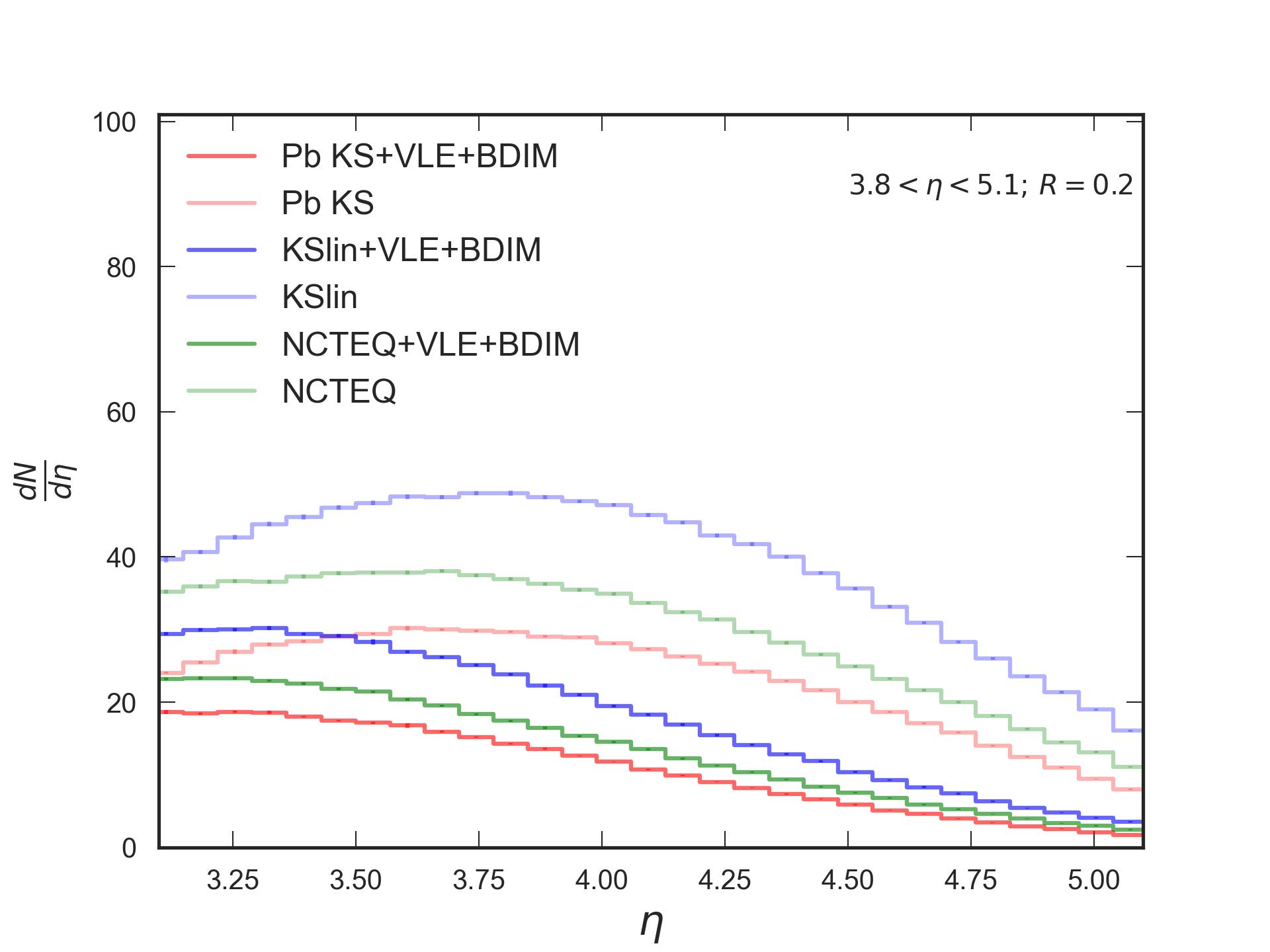
Figure 3: Comparisons of the rapidity distribution of jets for two different configurations of no-medium and medium case for the $\gamma$-jet input from PbPb collisions at $\sqrt{s}=5.02\,$TeV. The TMD grids are for all possible combinations of the saturation and Sudakov effects. The acceptances are: $3.8<y<5.2$, $p_{T}^{ini,\gamma}\geq 5\,$GeV and $p_{T}\geq 5\,$ GeV.

Figure 3 compares the distributions in rapidities of jets and photons obtained for the cases of in-medium jet propagation to the cases without in-medium jet-propagation obtained directly from KATIE for the different gluon TMDs. As can be seen, the presence of the jet–medium interactions leads overall to a considerable suppression of the rapidity distributions in comparison to the cases without the in-medium evolution. While the upper panel of Fig. 3 shows the rapidity distributions for jet particles undergoing only in-medium scatterings and medium-induced radiations, in the lower panel, the distributions that additionally include VLEs are presented. When the corresponding cases of the jet–medium interactions with and without VLEs are compared, the distributions with VLEs exhibit a stronger suppression for all the considered TMDs. Overall, the scenario that includes both the saturation and VLEs gives the largest suppression. Furthermore, it is quite close to the NCTEQ case because the Sudakov resummation was performed for both scenarios: NCTEQ and Pb KS.

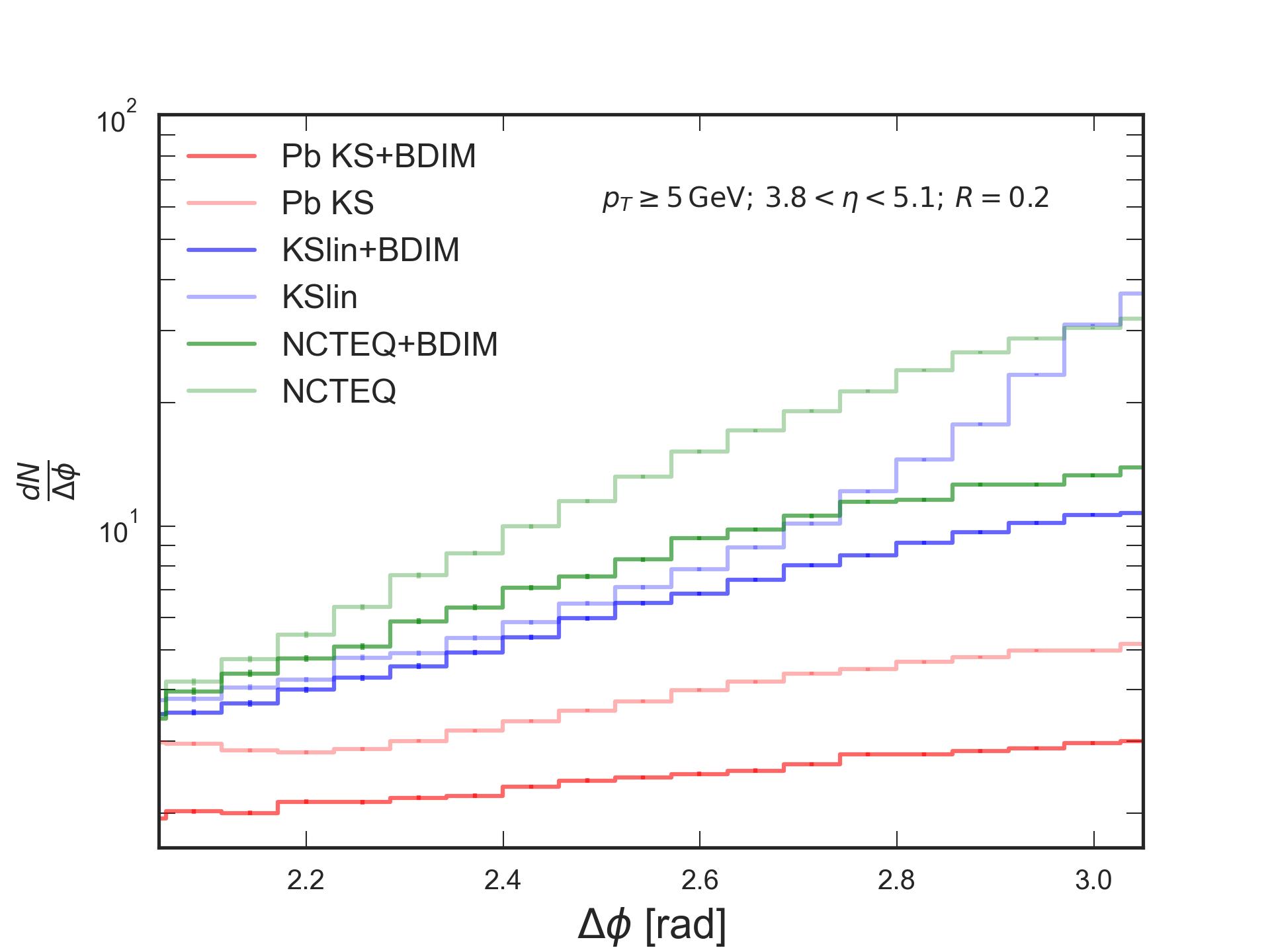
Figure 4: Comparisons of the azimuthal-angle decorrelations between jets and photons for different configurations of no-medium and medium case for $\gamma$–jet input from PbPb collisions at $\sqrt{s}=5.02\,$TeV. The TMD grids are for all possible combinations of the saturation and Sudakov effects. The acceptances are: $3.8<y<5.2$, $p_{T}^{ini,\gamma}\geq 5\,$GeV with $p_{T}\geq 5\,$GeV (top panel) and $p_{T}\geq 10\,$GeV (bottom panel).

Figure 4 shows the azimuthal-angle decorrelations for the jet–photon pairs, where the jets follow the BDIM evolution, in comparison to results without the in-medium jet evolution. The cases with the jet evolution exhibit a strong suppression at $\Delta\phi=\pi$, which becomes significantly less pronounced at smaller values of $\Delta\phi$ where the distributions with and without the jet–medium interactions start to converge. This invariance under the jet–medium interactions appears at larger values of $\Delta\phi$, if one rejects all the jet–photon pairs where $p_{T}$ of either the jet or the photon is below a certain value. One can explain such a behavior by the suppressed jet–medium interactions for jet-particles at large $p_{T}$. The observed behavior can be expected from a BDMPS-Z-type of coherent medium-induced emissions which are suppressed by a factor of $1/\sqrt{\omega}$ (where $\omega$ is the energy of the emitter). Furthermore, one can observe much more suppressed distributions for the TMDs with the saturation and the Sudakov resummation than for the results with the NCTEQ and KS-linear TMDs. This difference occurs both for the cases with and without the in-medium jet-evolution.

The results for the two observables discussed above, $\eta$ and $\Delta\phi$, indicate that both spectra are informative and carry valuable insights. Overall, our results suggest that the saturation effects may be observable in experimental analyses of jet-quenching in heavy-ion collisions.

5 Summary and conclusions

In summary, this work presents the first study of jet-quenching in the forward acceptance region of collider detectors, utilizing a combination of gluon-saturation dynamics and in-medium jet evolution. We find that the combination of non-perturbative saturation phenomena at early-stages followed by a perturbative regime through jet fragmentation should be employed to describe the upcoming AA-collision data at forward rapidities. As a concrete example, we have provided predictions suited to the kinematical cuts of the planned forward-calorimeter detector experiments. Furthermore, we have included a detailed description of the in-medium jet propagation through VLEs followed by the in-medium parton-branching process leading to the jet energy loss and intra-jet modifications. By comparing scenarios that combine the jet-quenching with the gluon saturation to those with the quenching but without the saturation, we demonstrate that the saturation effects are clearly evident in the observables we examine. This potentially may open new avenues to search for the saturation in the forward detectors. Finally, we demonstrate that VLEs provide the additional suppression of the cross section in nuclear collisions.

A qualitative understanding of the jet production in the $\gamma$–jet final state in the forward region provides an effective tool to study the flavor dependence in the forward rapidities, it also allows for an in-depth study of the role of selection biases as well as the path length dependence of the in-medium jet energy loss [91, 92, 93], as also pursued extensively in [94, 95, 96, 97].

The detailed methodology to include the saturation effects and the in-medium quenching presented here for the $\gamma$–jet configuration can be readily extended for generic dijet systems. In our study we have neglected glasma fields [98] which are expected to be relevant for early stages of heavy ion collisions and can lead to suppression of angular correlations [99]. The are however mostly contributing for processes where both of colliding ions are saturated and final states are produced in central rapidity region [100, 101, 102].

As an outlook, our study can be further developed by considering the possibility for implementing splitting kernels that account for a more realistic expansion scenario [82], as well as study through the framework of the resummed opacity expansion approach [103]. One can also study the same set up with recent Monte Carlo frameworks for modeling the jet–medium interactions, such as SUBA-jet [104]. Additionally, one could explore further by including the energy-smearing effects from the initial state radiation, as in Refs. [42, 43], for which the jet spectra can be significantly modified leading to a sizable effect on the jet nuclear modification factor ${R_{AA}}$. In this study, we have restricted ourselves to the lowest order in $\alpha_{s}$, leading to the transverse energy smearing function as a $\delta$-function due to the momentum conservation. We shall incorporate higher-order effects in detail in a future study.

Appendix A Uncertainties in observables

In order to estimate the influence of the jet-medium interactions on the studied observables, we have obtained some sample results for a medium temperature of $T=187.5$ MeV. The resulting values for the parameters $\hat{q}$, $n_{\rm med}$ and $m_{D}$ are:

$n_{\rm med}$	$\hat{q}$	$m_{D}$
$0.0338\,$GeV3	$0.1223\,$GeV${}^{2}/$fm	$0.4575\,$GeV

Fig. 5 shows the results for the jet nuclear modification factor $R_{AA}$ for jet evolution with VLEs and without VLEs in comparison to the previously shown results for $T=250$ MeV. As can be seen, the differences between the values of ${R_{AA}}$ with and without inclusion of the gluon saturation are in general larger than the differences resulting from a $25$% change of the medium temperature. Similar observations can be seen in the comparisons shown in Fig. 6 for the azimuthal-angle decorrelations.

Figure 5: Nuclear modification factors for media with the temperatures of $T=187.5\,$MeV and $T=250\,$MeV, respectively.

Figure 6: Azimuthal decorrelations for media with the temperatures of $T=187.5\,$MeV and $T=250\,$MeV, respectively.

Appendix B Monte Carlo algorithm for VLEs

In TMDICE, VLEs evolve following the DGLAP evolution equations for time-like final-state cascades, i.e.

$$Q^{2}\frac{\partial}{\partial Q^{2}}D_{q}(x,Q^{2}) =\frac{\alpha_{s}}{2\pi}\int dzP_{qq}(z)\left[\frac{1}{z}D_{q}\left(\frac{x}{z},Q^{2}\right)-D_{q}(x,Q^{2})\right]$$

$$+\frac{1}{z}P_{qg}(z)D_{g}\left(\frac{x}{z},Q^{2}\right)\,,$$ (31)

$$Q^{2}\frac{\partial}{\partial Q^{2}}D_{g}(x,Q^{2}) =\frac{\alpha_{s}}{2\pi}\int dzP_{gg}(z)\frac{1}{z}D_{g}\left(\frac{x}{z},Q^{2}\right)$$

$$+P_{gq}(z)\frac{1}{z}D_{q}\left(\frac{x}{z},Q^{2}\right)-\left[P_{gg}(z)+N_{F}P_{qg}(z)\right]$$

$$\times D_{g}(x,Q^{2})\,,$$ (32)

with the gluon and quark fragmentation functions $D_{g}(x,Q^{2})$ and $D_{q}(x,Q^{2})$, respectively. As with the BDIM evolution of jets, the running of the QCD coupling was neglected and $\alpha_{s}$ is given as a constant input parameter. The DGLAP evolution equations can be solved numerically via a Monte Carlo algorithm. To this end the Sudakov functions for the quark and the gluon are defined, respectively as

$$\Delta_{q}(Q_{1}^{2},Q_{2}^{2},E) =\exp\left[-\int_{Q_{2}^{2}}^{Q_{1}^{2}}\frac{dQ^{2}}{Q^{2}}\int_{x_{-}(Q^{2},E,R_{\rm max})}^{x_{+}(Q^{2},E)}dz\frac{\alpha_{s}}{2\pi}P_{qq}(z)\right]\,,$$ (33)

$$\Delta_{g}(Q_{1}^{2},Q_{2}^{2},E) =\exp\bigg{[}-\int_{Q_{2}^{2}}^{Q_{1}^{2}}\frac{dQ^{2}}{Q^{2}}\int_{x_{-}(Q^{2},E,R_{\rm max})}^{x_{+}(Q^{2},E,R_{\rm max})}dz\frac{\alpha_{s}}{2\pi}P_{gg}(z)$$

$$+N_{F}P_{qg}(z)\bigg{]}\,,$$ (34)

where $E$ is the energy of the quark or gluon, and we have introduced the integration boundaries $x_{\pm}(Q^{2},E,R_{\rm max})$, such that all possible parton splittings into particles on and off the mass-shell at angles smaller than a maximal angle $R_{\rm max}$ are considered. These boundaries are then given as

$$x_{\pm}(Q^{2},E,R_{\rm max})=\frac{1}{2}\left[1\pm\sqrt{1-\frac{2Q^{2}}{E^{2}(1-\cos R_{\rm max})}}\,\right]\,.$$ (35)

For partonic cascades, the above integration boundaries would allow to consider angular ordering, if $R_{\rm max}$ is always adapted to the previous branching angle. In the current work, however, $R_{\rm max}$ is considered as a global maximal angle given as a parameter in Table 1. The following CDFs are defined for the splitting functions of a particle $j$ into a particle $i$

$$\rho_{ij}(z,Q_{i}^{2},E_{i})=\int_{x_{-}(Q_{i}^{2},E_{i},R_{\rm max})}^{z}d\tilde{z}P_{ij}(\tilde{z})\,.$$ (36)

It is then possible to create a Monte Carlo algorithm that generates jets from initial partons, where the fragmentation functions obey Eqs. (31) and (32), as was done in many earlier works [105, 106, 107]. The jet particles are specified by their type (i.e. whether they are quarks or gluons) and their four-momenta. The algorithm starts from a given initial jet parton. Then, for any jet parton $A$, it is determined whether a splitting occurs, and in such a case the splitting products $B$ and $C$ are obtained. This process is repeated for the splitting products $B$ and $C$, and for their possible products, etc., resulting in a parton cascade. Once no splitting occurs for any of the considered particles, the algorithm automatically stops. Then, it is still possible for particles to undergo the BDIM evolution inside the medium – this is discussed later on. The following few steps give the part of the algorithm that generates the splitting products $B$ and $C$ from the parton $A$ which is presumed to split:

1. It is determined, whether the splitting produces a quark–antiquark pair. If the parton $A$ is a quark, it decays into a quark and a gluon, otherwise a random number $R_{t}\in[0,1]$ is selected and compared to the ratio

   $$p_{t}(Q_{A}^{2},E_{A})=\left[{1+\frac{\rho_{qg}(x_{+}(Q_{A}^{2},E_{A},R_{\rm max}),Q_{A}^{2},E_{A})}{\rho_{gg}(x_{+}(Q_{A}^{2},E_{A},R_{\rm max}),Q_{A}^{2},E_{A})}}\right]^{-1}\,.$$ (37)

   If $R_{t}\leq p_{t}(Q_{A}^{2},E_{A})$ a gluon-pair is produced, otherwise a quark–antiquark pair.

2. The energy fraction $z_{B}=E_{B}/E_{A}$ is obtained by selecting a random number $R_{z}\in[0,1]$ and solving the equation

   $$R_{z}=\frac{\rho_{BA}(z_{B},Q_{A}^{2},E_{A},R_{\rm max})}{\rho_{BA}(x_{+}(Q_{A}^{2},E_{A}),Q_{A}^{2},E_{A})}\,.$$ (38)

   The energy fraction of the other particle $z_{C}=E_{C}/E_{A}$ is obtained from the energy conservation: $z_{C}=1-z_{B}$.

3. The squared virtualities $Q_{i}^{2}$ ($i=B,\,C$) of the particles $B$ and $C$ are selected in such a way that they follow the probability distribution functions $p_{i}(Q_{A}^{2},Q_{i}^{2},E_{A})$ given by

   $$p_{i}(Q_{A}^{2},Q_{i}^{2},E_{A})=\frac{\partial}{\partial Q_{i}^{2}}\Delta_{i}(Q_{A}^{2},Q_{i}^{2},E_{A})\,,$$ (39)

   i.e. obeying the CDFs of the Sudakov functions of Eqs. (33) and (34). This selection process is done via a veto algorithm (cf. [107] for details). For the selection of the squared virtuality $Q_{i}^{2}$, the distributions

   $$\tilde{\Delta}_{q}(Q_{1}^{2},Q_{2}^{2}) =\exp\left[-\int_{Q_{2}^{2}}^{Q_{1}^{2}}\frac{dQ^{2}}{Q^{2}}\int_{\epsilon_{\rm VLE}}^{1-{\epsilon_{\rm VLE}}}dz\frac{\alpha_{s}}{2\pi}P_{qq}(z)\right]\,,$$ (40)

   $$\tilde{\Delta}_{g}(Q_{1}^{2},Q_{2}^{2}) =\exp\bigg{[}-\int_{Q_{2}^{2}}^{Q_{1}^{2}}\frac{dQ^{2}}{Q^{2}}\int_{\epsilon_{\rm VLE}}^{1-{\epsilon_{\rm VLE}}}dz\frac{\alpha_{s}}{2\pi}P_{gg}(z)$$

   $$+N_{F}P_{qg}(z)\bigg{]}\,,$$ (41)

   with the numerical parameter $\epsilon_{\rm VLE}$ given in Table 1, are used as CDFs. However, an additional rejection condition is applied, which ensures that the values selected for $Q_{i}^{2}$ obey the CDFs of Eqs. (33) and (34).

4. The components of momenta of the particles $B$ and $C$ transverse to the momentum of particle $A$ are calculated as

   $$k_{\perp BC}^{2} =\frac{1}{\sqrt{1-\frac{Q_{A}^{2}}{E_{A}^{2}}}}\left[z_{B}(1-z_{B})Q_{A}^{2}-(1-z_{B})Q_{B}^{2}-z_{B}Q_{C}^{2}\right.$$

   $$\left.-\frac{1}{4E_{A}^{2}}\left(Q_{A}^{4}+Q_{B}^{4}+Q_{C}^{4}-2Q_{A}^{2}Q_{B}^{2}-2Q_{A}^{2}Q_{C}^{2}-2Q_{B}^{2}Q_{C}^{2}\right)\right]\,,$$ (42)

   If $k_{\perp\,BC}^{2}<0$, steps 1 to 3 are repeated.

5. An azimuthal angle $\phi$ of the transverse momentum of particle $B$ with regard to the momentum of the particle $A$ is selected randomly from the uniform distribution in the range $[0,2\pi]$. The corresponding angle for the particle $C$ is obtained as $\phi_{C}=\phi+\pi$. Thus, azimuthal correlations between the subsequent splittings are neglected in this algorithm.

6. Four-momenta of the particles $B$ and $C$ are calculated from the four-momentum of the particle $A$ and from the previously obtained variables $z_{B}$, $Q_{B}$, $Q_{C}$, $k_{\perp BC}^{2}$ and $\phi$, as described in a more detail in B.1 below.

After the splitting of the parton $A$ into the partons $B$ and $C$, the four-momenta of the three particles are used to evaluate phase-space constraints that are outlined below in B.2. If the phase-space constraints are fulfilled, the partons $B$ and $C$ also split and the steps 1 to 6 in the list above are repeated for the partons $B$ and $C$. Otherwise, it is presumed that the splitting does not take place and the particle $A$ is considered as the final particle that does not undergo further evolution in the vacuum. The jet evolution by VLEs stops once all the generated particles are the final particles.

B.1 Kinematical descriptions of particle four-momenta

For jets evolving via VLEs, the four-momentum of the a parton $A$ branching into partons $B$ and $C$ is known. The four-momenta of the particles $B$ and $C$ are determined by the four-momentum conservation and the selected values $z_{B}$ (and $z_{C}=1-z_{B}$), $Q_{B}$, $Q_{C}$ and $\phi$ (the four-momentum conservation then yields the azimuthal angle for the particle $C$, $\phi_{C}=\phi+\pi$ and $k_{\perp BC}^{2}$ as given in Eq. (42)). In the reference frame where the z-axis is in the same direction as the three-momentum of the particle $A$, the four-momenta of the particles $A$, $B$ and $C$ are obtained as

$$p_{A,\,\mathrm{local}} =\left(E_{A},0,0,\sqrt{E_{A}^{2}-Q_{A}^{2}}\,\right)\,,$$ (43)

$$p_{B,\,\mathrm{local}} =\bigg{(}z_{B}\,E_{A},\,k_{\perp BC}\cos\phi,\,k_{\perp BC}\sin\phi,$$

$$\hskip 17.07164pt\sqrt{z_{B}^{2}E_{A}^{2}-k_{\perp BC}^{2}-Q_{B}^{2}}\,\bigg{)}\,,$$ (44)

$$p_{C,\,\mathrm{local}} =\bigg{(}z_{C}E_{A},-k_{\perp BC}\cos\phi,-k_{\perp BC}\sin\phi,$$

$$\hskip 17.07164pt\sqrt{z_{C}^{2}E_{A}^{2}-k_{\perp BC}^{2}-Q_{C}^{2}}\,\bigg{)}\,.$$ (45)

The parton momenta $p_{B,\,\mathrm{local}}$ and $p_{C,\,\mathrm{local}}$ are then rotated into a global reference frame – the LAB frame of the collision. The four-momentum of the particle $A$ in the LAB frame $p_{A,\,\mathrm{LAB}}$ is already known and, thus, the rotation $\hat{R}_{\mathrm{local}\,\rightarrow\,\mathrm{LAB}}$ that transforms $p_{A,\,\mathrm{local}}$ into $p_{A,\,\mathrm{LAB}}$ is also known. Thus, one obtains

$$p_{B,\,\mathrm{LAB}} =\hat{R}_{\mathrm{local}\,\rightarrow\,\mathrm{LAB}}\,p_{B,\,\mathrm{local}},$$ (46)

$$p_{C,\,\mathrm{LAB}} =\hat{R}_{\mathrm{local}\,\rightarrow\,\mathrm{LAB}}\,p_{C,\,\mathrm{local}}.$$ (47)

B.2 Phase-space constraints of VLEs and their implementations

In TMDICE, after every branching of a parton $A$ into partons $B$ and $C$ due to VLEs is simulated, it is verified whether that branching fulfills certain phase-space conditions. Only the parton branchings that fulfill the phase-space constraints are considered to contribute to the jet-evolution. If a parton branching violates the phase-space constraints, the parton $A$ is considered as the final particle that does not undergo further evolution by VLEs. However, the parton $A$ may still undergo further evolution in a medium by scatterings and medium-induced emissions. The phase-space constraints are:

• It is tested whether Eq. (14) holds for the particle $A$.

• It is tested whether Eq. (15) holds for the particle $A$.

• It is tested whether

  $$k_{\perp\,BC}>k_{\perp\,\,\mathrm{min}}\,,$$ (48)

  where $k_{\perp\,\,\mathrm{min}}$ is a manually set threshold value.

A particle that violates any of the three conditions described above via Eqs. (14), (15) and (48) does no longer evolve via VLEs. However, it is possible that these final particles from VLEs still evolve via the medium-induced radiation and the scattering in the medium. To this end, all the final particles from VLEs above a certain threshold value $x_{\mathrm{min\,VLE}}$ of the energy fraction $x$ are considered the initial particles of the parton cascades formed via the medium-induced radiation and the scattering in the medium.

It is also possible that the final particles of the VLE evolution are still off-mass-shell. Then, after evolving in the medium, parton emissions outside the medium may occur as a possible third stage of the jet evolution [55]. In the current work, we neglect such a third stage and set virtualites of the final particles of the VLE evolution to $0$. As a consequence of the vanishing parton virtualities, the particle four-momenta need to be reevaluated in the following way: If the parton $A$ splits into the partons $B$ and $C$, and the parton $B$ is the final particle from VLEs, then we set $Q_{B}=0$ and recalculate $k_{T}$ according to Eq. (42). Then, Eqs. (44)–(47) are evaluated again, yielding new values for the four-momenta of the particles $B$ and $C$.

References

- [1] L. V. Gribov, E. M. Levin, M. G. Ryskin, Semihard Processes in QCD, Phys. Rept. 100 (1983) 1–150. doi:10.1016/0370-1573(83)90022-4.
- [2] F. Gelis, E. Iancu, J. Jalilian-Marian, R. Venugopalan, The Color Glass Condensate, Ann. Rev. Nucl. Part. Sci. 60 (2010) 463–489. arXiv:1002.0333, doi:10.1146/annurev.nucl.010909.083629.
-
[3]
Y. V. Kovchegov, E. Levin, Quantum chromodynamics at high energy, Vol. 33, Cambridge University Press, 2012.
URL http://www.cambridge.org/de/knowledge/isbn/item6803159 - [4] J. Adams, et al., Forward neutral pion production in p+p and d+Au collisions at s(NN)**(1/2) = 200-GeV, Phys. Rev. Lett. 97 (2006) 152302. arXiv:nucl-ex/0602011, doi:10.1103/PhysRevLett.97.152302.
- [5] A. Adare, et al., Suppression of back-to-back hadron pairs at forward rapidity in Au Collisions at GeV, Phys. Rev. Lett. 107 (2011) 172301. arXiv:1105.5112, doi:10.1103/PhysRevLett.107.172301.
- [6] M. S. Abdallah, et al., Evidence for Nonlinear Gluon Effects in QCD and Their Mass Number Dependence at STAR, Phys. Rev. Lett. 129 (9) (2022) 092501. arXiv:2111.10396, doi:10.1103/PhysRevLett.129.092501.
- [7] K. J. Golec-Biernat, M. Wusthoff, Saturation effects in deep inelastic scattering at low Q**2 and its implications on diffraction, Phys. Rev. D 59 (1998) 014017. arXiv:hep-ph/9807513, doi:10.1103/PhysRevD.59.014017.
- [8] T. Lappi, H. Mantysaari, Forward dihadron correlations in deuteron-gold collisions with the Gaussian approximation of JIMWLK, Nucl. Phys. A 908 (2013) 51–72. arXiv:1209.2853, doi:10.1016/j.nuclphysa.2013.03.017.
- [9] B. Ducloué, T. Lappi, H. Mäntysaari, Isolated photon production in proton-nucleus collisions at forward rapidity, Phys. Rev. D 97 (5) (2018) 054023. arXiv:1710.02206, doi:10.1103/PhysRevD.97.054023.
- [10] J. L. Albacete, G. Giacalone, C. Marquet, M. Matas, Forward dihadron back-to-back correlations in collisions, Phys. Rev. D 99 (1) (2019) 014002. arXiv:1805.05711, doi:10.1103/PhysRevD.99.014002.
- [11] B. Ducloué, T. Lappi, H. Mäntysaari, Forward and meson nuclear suppression at the LHC, Nucl. Part. Phys. Proc. 289-290 (2017) 309–312. arXiv:1612.04585, doi:10.1016/j.nuclphysbps.2017.05.071.
- [12] A. Stasto, S.-Y. Wei, B.-W. Xiao, F. Yuan, On the Dihadron Angular Correlations in Forward collisions, Phys. Lett. B 784 (2018) 301–306. arXiv:1805.05712, doi:10.1016/j.physletb.2018.08.011.
- [13] A. van Hameren, P. Kotko, K. Kutak, S. Sapeta, Broadening and saturation effects in dijet azimuthal correlations in p-p and p-Pb collisions at 5.02 TeV, Phys. Lett. B 795 (2019) 511–515. arXiv:1903.01361, doi:10.1016/j.physletb.2019.06.055.
- [14] S. Benić, O. Garcia-Montero, A. Perkov, Isolated photon-hadron production in high energy pp and pA collisions at RHIC and LHC, Phys. Rev. D 105 (11) (2022) 114052. arXiv:2203.01685, doi:10.1103/PhysRevD.105.114052.
- [15] ALICE Collaboration, Physics of the ALICE Forward Calorimeter upgrade, ALICE-PUBLIC-2023-001 (2023).
-
[16]
ALICE Collaboration, Letter of Intent for an ALICE Forward Calorimeter (FoCal) (2020).
URL https://cds.cern.ch/record/2728667 - [17] A. Dumitru, A. Hayashigaki, J. Jalilian-Marian, The Color glass condensate and hadron production in the forward region, Nucl. Phys. A 765 (2006) 464–482. arXiv:hep-ph/0506308, doi:10.1016/j.nuclphysa.2005.11.014.
- [18] C. Marquet, Forward inclusive dijet production and azimuthal correlations in p(A) collisions, Nucl. Phys. A 796 (2007) 41–60. arXiv:0708.0231, doi:10.1016/j.nuclphysa.2007.09.001.
- [19] A. van Hameren, P. Kotko, K. Kutak, C. Marquet, E. Petreska, S. Sapeta, Forward di-jet production in p+Pb collisions in the small-x improved TMD factorization framework, JHEP 12 (2016) 034, [Erratum: JHEP 02, 158 (2019)]. arXiv:1607.03121, doi:10.1007/JHEP12(2016)034.
- [20] P. Jucha, M. Kłusek-Gawenda, A. Szczurek, Light-by-light scattering in ultraperipheral collisions of heavy ions at two future detectors, Phys. Rev. D 109 (1) (2024) 014004. arXiv:2308.01550, doi:10.1103/PhysRevD.109.014004.
- [21] I. Ganguli, A. van Hameren, P. Kotko, K. Kutak, Forward +jet production in proton-proton and proton-lead collisions at LHC within the FoCal calorimeter acceptance, Eur. Phys. J. C 83 (9) (2023) 868. arXiv:2306.04706, doi:10.1140/epjc/s10052-023-12043-3.
- [22] A. van Hameren, H. Kakkad, P. Kotko, K. Kutak, S. Sapeta, Searching for saturation in forward dijet production at the LHC, Eur. Phys. J. C 83 (10) (2023) 947. arXiv:2306.17513, doi:10.1140/epjc/s10052-023-12120-7.
- [23] T. Altinoluk, C. Marquet, P. Taels, Low-x improved TMD approach to the lepto- and hadroproduction of a heavy-quark pair, JHEP 06 (2021) 085. arXiv:2103.14495, doi:10.1007/JHEP06(2021)085.
- [24] H. Fujii, C. Marquet, K. Watanabe, Comparison of improved TMD and CGC frameworks in forward quark dijet production, JHEP 12 (2020) 181. arXiv:2006.16279, doi:10.1007/JHEP12(2020)181.
- [25] A. Morreale, F. Salazar, Mining for Gluon Saturation at Colliders, Universe 7 (8) (2021) 312. arXiv:2108.08254, doi:10.3390/universe7080312.
- [26] E. V. Shuryak, Quark-Gluon Plasma and Hadronic Production of Leptons, Photons and Psions, Phys. Lett. B 78 (1978) 150. doi:10.1016/0370-2693(78)90370-2.
- [27] E. V. Shuryak, What RHIC experiments and theory tell us about properties of quark-gluon plasma?, Nucl. Phys. A 750 (2005) 64–83. arXiv:hep-ph/0405066, doi:10.1016/j.nuclphysa.2004.10.022.
- [28] K. Kutak, S. Sapeta, Gluon saturation in dijet production in p-Pb collisions at Large Hadron Collider, Phys. Rev. D 86 (2012) 094043. arXiv:1205.5035, doi:10.1103/PhysRevD.86.094043.
-
[29]
G. Aad, et al., The ATLAS Experiment at the CERN Large Hadron Collider, JINST 3 (2008) S08003.
doi:10.1088/1748-0221/3/08/S08003.
URL https://iopscience.iop.org/article/10.1088/1748-0221/3/08/S08003 -
[30]
S. Chatrchyan, et al., The CMS experiment at the CERN LHC, JINST 3 (2008) S08004.
doi:10.1088/1748-0221/3/08/S08004.
URL https://iopscience.iop.org/article/10.1088/1748-0221/3/08/S08004 - [31] D. A. Appel, Jets as a Probe of Quark - Gluon Plasmas, Phys. Rev. D 33 (1986) 717. doi:10.1103/PhysRevD.33.717.
- [32] J. P. Blaizot, L. D. McLerran, Jets in Expanding Quark - Gluon Plasmas, Phys. Rev. D 34 (1986) 2739. doi:10.1103/PhysRevD.34.2739.
- [33] M. Gyulassy, M. Plumer, Jet Quenching in Dense Matter, Phys. Lett. B 243 (1990) 432–438. doi:10.1016/0370-2693(90)91409-5.
- [34] X.-N. Wang, M. Gyulassy, Gluon shadowing and jet quenching in A + A collisions at s**(1/2) = 200-GeV, Phys. Rev. Lett. 68 (1992) 1480–1483. doi:10.1103/PhysRevLett.68.1480.
- [35] R. Baier, Y. L. Dokshitzer, A. H. Mueller, S. Peigne, D. Schiff, Radiative energy loss and p(T) broadening of high-energy partons in nuclei, Nucl. Phys. B 484 (1997) 265–282. arXiv:hep-ph/9608322, doi:10.1016/S0550-3213(96)00581-0.
- [36] B. G. Zakharov, Radiative energy loss of high-energy quarks in finite size nuclear matter and quark - gluon plasma, JETP Lett. 65 (1997) 615–620. arXiv:hep-ph/9704255, doi:10.1134/1.567389.
- [37] R. B. Neufeld, I. Vitev, B. W. Zhang, The Physics of -tagged jets at the LHC, Phys. Rev. C 83 (2011) 034902. arXiv:1006.2389, doi:10.1103/PhysRevC.83.034902.
- [38] S. P. Adhya, K. Kutak, W. Płaczek, M. Rohrmoser, K. Tywoniuk, Transverse momentum broadening of medium-induced cascades in expanding media, Eur. Phys. J. C 83 (6) (2023) 512. arXiv:2211.15803, doi:10.1140/epjc/s10052-023-11555-2.
- [39] S. P. Adhya, K. Tywoniuk, Sensitivity of jet quenching to the initial state in heavy-ion collisions (9 2024). arXiv:2409.04295.
- [40] S. Chatrchyan, et al., Observation and studies of jet quenching in PbPb collisions at nucleon-nucleon center-of-mass energy = 2.76 TeV, Phys. Rev. C 84 (2011) 024906. arXiv:1102.1957, doi:10.1103/PhysRevC.84.024906.
- [41] G. Aad, et al., Observation of a Centrality-Dependent Dijet Asymmetry in Lead-Lead Collisions at TeV with the ATLAS Detector at the LHC, Phys. Rev. Lett. 105 (2010) 252303. arXiv:1011.6182, doi:10.1103/PhysRevLett.105.252303.
- [42] X.-N. Wang, Z. Huang, I. Sarcevic, Jet quenching in the opposite direction of a tagged photon in high-energy heavy ion collisions, Phys. Rev. Lett. 77 (1996) 231–234. arXiv:hep-ph/9605213, doi:10.1103/PhysRevLett.77.231.
- [43] X.-N. Wang, Z. Huang, Study medium induced parton energy loss in gamma + jet events of high-energy heavy ion collisions, Phys. Rev. C 55 (1997) 3047–3061. arXiv:hep-ph/9701227, doi:10.1103/PhysRevC.55.3047.
- [44] A. Ogrodnik, M. Rybář, M. Spousta, Flavor and path-length dependence of jet quenching from inclusive jet and -jet suppression (7 2024). arXiv:2407.11234.
- [45] P. Kotko, K. Kutak, C. Marquet, E. Petreska, S. Sapeta, A. van Hameren, Improved TMD factorization for forward dijet production in dilute-dense hadronic collisions, JHEP 09 (2015) 106. arXiv:1503.03421, doi:10.1007/JHEP09(2015)106.
- [46] T. Altinoluk, R. Boussarie, P. Kotko, Interplay of the CGC and TMD frameworks to all orders in kinematic twist, JHEP 05 (2019) 156. arXiv:1901.01175, doi:10.1007/JHEP05(2019)156.
- [47] A. H. Rezaeian, Semi-inclusive photon-hadron production in pp and pA collisions at RHIC and LHC, Phys. Rev. D 86 (2012) 094016. arXiv:1209.0478, doi:10.1103/PhysRevD.86.094016.
- [48] J. Jalilian-Marian, A. H. Rezaeian, Prompt photon production and photon-hadron correlations at RHIC and the LHC from the Color Glass Condensate, Phys. Rev. D 86 (2012) 034016. arXiv:1204.1319, doi:10.1103/PhysRevD.86.034016.
- [49] M. Deak, F. Hautmann, H. Jung, K. Kutak, Forward Jet Production at the Large Hadron Collider, JHEP 09 (2009) 121. arXiv:0908.0538, doi:10.1088/1126-6708/2009/09/121.
- [50] I. Balitsky, Operator expansion for high-energy scattering, Nucl. Phys. B 463 (1996) 99–160. arXiv:hep-ph/9509348, doi:10.1016/0550-3213(95)00638-9.
- [51] Y. V. Kovchegov, Small x F(2) structure function of a nucleus including multiple pomeron exchanges, Phys. Rev. D 60 (1999) 034008. arXiv:hep-ph/9901281, doi:10.1103/PhysRevD.60.034008.
- [52] A. Mueller, B.-W. Xiao, F. Yuan, Sudakov double logarithms resummation in hard processes in the small-x saturation formalism, Phys. Rev. D 88 (11) (2013) 114010. arXiv:1308.2993, doi:10.1103/PhysRevD.88.114010.
- [53] A. H. Mueller, B.-W. Xiao, F. Yuan, Sudakov Resummation in Small- Saturation Formalism, Phys. Rev. Lett. 110 (8) (2013) 082301. arXiv:1210.5792, doi:10.1103/PhysRevLett.110.082301.
- [54] M. A. Al-Mashad, A. van Hameren, H. Kakkad, P. Kotko, K. Kutak, P. van Mechelen, S. Sapeta, Dijet azimuthal correlations in p-p and p-Pb collisions at forward LHC calorimeters, JHEP 12 (2022) 131. arXiv:2210.06613, doi:10.1007/JHEP12(2022)131.
- [55] P. Caucal, E. Iancu, A. H. Mueller, G. Soyez, Vacuum-like jet fragmentation in a dense QCD medium, Phys. Rev. Lett. 120 (2018) 232001. arXiv:1801.09703, doi:10.1103/PhysRevLett.120.232001.
- [56] Y. Mehtar-Tani, C. A. Salgado, K. Tywoniuk, The Radiation pattern of a QCD antenna in a dense medium, JHEP 10 (2012) 197. arXiv:1205.5739, doi:10.1007/JHEP10(2012)197.
- [57] V. N. Gribov, L. N. Lipatov, Deep inelastic e p scattering in perturbation theory, Sov. J. Nucl. Phys. 15 (1972) 438–450.
- [58] G. Altarelli, G. Parisi, Asymptotic Freedom in Parton Language, Nucl. Phys. B 126 (1977) 298–318. doi:10.1016/0550-3213(77)90384-4.
- [59] Y. L. Dokshitzer, Calculation of the Structure Functions for Deep Inelastic Scattering and e+ e- Annihilation by Perturbation Theory in Quantum Chromodynamics., Sov. Phys. JETP 46 (1977) 641–653.
- [60] J.-P. Blaizot, F. Dominguez, E. Iancu, Y. Mehtar-Tani, Medium-induced gluon branching, JHEP 01 (2013) 143. arXiv:1209.4585, doi:10.1007/JHEP01(2013)143.
- [61] J.-P. Blaizot, F. Dominguez, E. Iancu, Y. Mehtar-Tani, Probabilistic picture for medium-induced jet evolution, JHEP 06 (2014) 075. arXiv:1311.5823, doi:10.1007/JHEP06(2014)075.
- [62] E. Blanco, K. Kutak, W. Placzek, M. Rohrmoser, K. Tywoniuk, System of evolution equations for quark and gluon jet quenching with broadening, Eur. Phys. J. C 82 (4) (2022) 355. arXiv:2109.05918, doi:10.1140/epjc/s10052-022-10311-2.
- [63] M. Dasgupta, F. Dreyer, G. P. Salam, G. Soyez, Small-radius jets to all orders in QCD, JHEP 04 (2015) 039. arXiv:1411.5182, doi:10.1007/JHEP04(2015)039.
- [64] M. Dasgupta, F. A. Dreyer, G. P. Salam, G. Soyez, Inclusive jet spectrum for small-radius jets, JHEP 06 (2016) 057. arXiv:1602.01110, doi:10.1007/JHEP06(2016)057.
- [65] Z.-B. Kang, F. Ringer, I. Vitev, The semi-inclusive jet function in SCET and small radius resummation for inclusive jet production, JHEP 10 (2016) 125. arXiv:1606.06732, doi:10.1007/JHEP10(2016)125.
- [66] Y. Mehtar-Tani, K. Tywoniuk, Sudakov suppression of jets in QCD media, Phys. Rev. D 98 (5) (2018) 051501. arXiv:1707.07361, doi:10.1103/PhysRevD.98.051501.
- [67] F. Domínguez, J. G. Milhano, C. A. Salgado, K. Tywoniuk, V. Vila, Mapping collinear in-medium parton splittings, Eur. Phys. J. C 80 (1) (2020) 11. arXiv:1907.03653, doi:10.1140/epjc/s10052-019-7563-0.
- [68] Y. Mehtar-Tani, D. Pablos, K. Tywoniuk, Jet suppression and azimuthal anisotropy from RHIC to LHC, Phys. Rev. D 110 (1) (2024) 014009. arXiv:2402.07869, doi:10.1103/PhysRevD.110.014009.
- [69] J. Casalderrey-Solana, Z. Hulcher, G. Milhano, D. Pablos, K. Rajagopal, Simultaneous description of hadron and jet suppression in heavy-ion collisions, Phys. Rev. C 99 (5) (2019) 051901. arXiv:1808.07386, doi:10.1103/PhysRevC.99.051901.
- [70] J. Casalderrey-Solana, G. Milhano, D. Pablos, K. Rajagopal, Modification of Jet Substructure in Heavy Ion Collisions as a Probe of the Resolution Length of Quark-Gluon Plasma, JHEP 01 (2020) 044. arXiv:1907.11248, doi:10.1007/JHEP01(2020)044.
- [71] P. Caucal, E. Iancu, G. Soyez, Deciphering the distribution in ultrarelativistic heavy ion collisions, JHEP 10 (2019) 273. arXiv:1907.04866, doi:10.1007/JHEP10(2019)273.
- [72] Y. Mehtar-Tani, C. A. Salgado, K. Tywoniuk, Jets in QCD Media: From Color Coherence to Decoherence, Phys. Lett. B 707 (2012) 156–159. arXiv:1102.4317, doi:10.1016/j.physletb.2011.12.042.
- [73] S. P. Adhya, C. A. Salgado, M. Spousta, K. Tywoniuk, Multi-partonic medium induced cascades in expanding media, Eur. Phys. J. C 82 (1) (2022) 20. arXiv:2106.02592, doi:10.1140/epjc/s10052-021-09950-8.
- [74] Y. Mehtar-Tani, C. A. Salgado, K. Tywoniuk, The radiation pattern of a QCD antenna in a dilute medium, JHEP 04 (2012) 064. arXiv:1112.5031, doi:10.1007/JHEP04(2012)064.
- [75] R. Baier, Y. L. Dokshitzer, S. Peigne, D. Schiff, Induced gluon radiation in a QCD medium, Phys. Lett. B345 (1995) 277–286. arXiv:hep-ph/9411409, doi:10.1016/0370-2693(94)01617-L.
- [76] R. Baier, Y. L. Dokshitzer, A. H. Mueller, S. Peigne, D. Schiff, The Landau-Pomeranchuk-Migdal effect in QED, Nucl. Phys. B478 (1996) 577–597. arXiv:hep-ph/9604327, doi:10.1016/0550-3213(96)00426-9.
- [77] R. Baier, D. Schiff, B. G. Zakharov, Energy loss in perturbative QCD, Ann. Rev. Nucl. Part. Sci. 50 (2000) 37–69. arXiv:hep-ph/0002198, doi:10.1146/annurev.nucl.50.1.37.
- [78] R. Baier, A. H. Mueller, D. Schiff, D. T. Son, ’Bottom up’ thermalization in heavy ion collisions, Phys. Lett. B502 (2001) 51–58. arXiv:hep-ph/0009237, doi:10.1016/S0370-2693(01)00191-5.
- [79] B. G. Zakharov, Fully quantum treatment of the Landau-Pomeranchuk-Migdal effect in QED and QCD, JETP Lett. 63 (1996) 952–957. arXiv:hep-ph/9607440, doi:10.1134/1.567126.
- [80] B. G. Zakharov, Transverse spectra of radiation processes in-medium, JETP Lett. 70 (1999) 176–182. arXiv:hep-ph/9906536, doi:10.1134/1.568149.
- [81] R. Baier, Y. L. Dokshitzer, A. H. Mueller, S. Peigne, D. Schiff, Radiative energy loss of high-energy quarks and gluons in a finite volume quark - gluon plasma, Nucl. Phys. B 483 (1997) 291–320. arXiv:hep-ph/9607355, doi:10.1016/S0550-3213(96)00553-6.
- [82] S. P. Adhya, C. A. Salgado, M. Spousta, K. Tywoniuk, Medium-induced cascade in expanding media, JHEP 07 (2020) 150. arXiv:1911.12193, doi:10.1007/JHEP07(2020)150.
- [83] M. Rohrmoser, The TMDICE Monte Carlo shower program and algorithm for jet-fragmentation via coherent medium induced radiations and scattering, Comput. Phys. Commun. 276 (2022) 108343. arXiv:2111.00323, doi:10.1016/j.cpc.2022.108343.
- [84] A. van Hameren, KaTie : For parton-level event generation with -dependent initial states, Comput. Phys. Commun. 224 (2018) 371–380. arXiv:1611.00680, doi:10.1016/j.cpc.2017.11.005.
- [85] J. Kwiecinski, A. D. Martin, A. M. Stasto, A Unified BFKL and GLAP description of F2 data, Phys. Rev. D 56 (1997) 3991–4006. arXiv:hep-ph/9703445, doi:10.1103/PhysRevD.56.3991.
- [86] E. Blanco, A. van Hameren, H. Jung, A. Kusina, K. Kutak, boson production in proton-lead collisions at the LHC accounting for transverse momenta of initial partons, Phys. Rev. D 100 (5) (2019) 054023. arXiv:1905.07331, doi:10.1103/PhysRevD.100.054023.
- [87] K. Kovarik, et al., nCTEQ15 - Global analysis of nuclear parton distributions with uncertainties in the CTEQ framework, Phys. Rev. D 93 (8) (2016) 085037. arXiv:1509.00792, doi:10.1103/PhysRevD.93.085037.
- [88] A. van Hameren, K. Kutak, W. Płaczek, M. Rohrmoser, K. Tywoniuk, Jet quenching and effects of non-Gaussian transverse-momentum broadening on dijet observables, Phys. Rev. C 102 (4) (2020) 044910. arXiv:1911.05463, doi:10.1103/PhysRevC.102.044910.
- [89] M. Cacciari, G. P. Salam, G. Soyez, FastJet User Manual, Eur. Phys. J. C 72 (2012) 1896. arXiv:1111.6097, doi:10.1140/epjc/s10052-012-1896-2.
- [90] M. Cacciari, G. P. Salam, Dispelling the myth for the jet-finder, Phys. Lett. B 641 (2006) 57–61. arXiv:hep-ph/0512210, doi:10.1016/j.physletb.2006.08.037.
- [91] H. Zhang, J. F. Owens, E. Wang, X.-N. Wang, Tomography of high-energy nuclear collisions with photon-hadron correlations, Phys. Rev. Lett. 103 (2009) 032302. arXiv:0902.4000, doi:10.1103/PhysRevLett.103.032302.
- [92] G.-Y. Qin, J. Ruppert, C. Gale, S. Jeon, G. D. Moore, Jet energy loss, photon production, and photon-hadron correlations at RHIC, Phys. Rev. C 80 (2009) 054909. arXiv:0906.3280, doi:10.1103/PhysRevC.80.054909.
- [93] T. Renk, Towards jet tomography: gamma-hadron correlations, Phys. Rev. C 74 (2006) 034906. arXiv:hep-ph/0607166, doi:10.1103/PhysRevC.74.034906.
- [94] B. Betz, M. Gyulassy, Constraints on the Path-Length Dependence of Jet Quenching in Nuclear Collisions at RHIC and LHC, JHEP 08 (2014) 090, [Erratum: JHEP 10, 043 (2014)]. arXiv:1404.6378, doi:10.1007/JHEP10(2014)043.
- [95] B. Betz, M. Gyulassy, M. Luzum, J. Noronha, J. Noronha-Hostler, I. Portillo, C. Ratti, Cumulants and nonlinear response of high harmonic flow at TeV, Phys. Rev. C 95 (4) (2017) 044901. arXiv:1609.05171, doi:10.1103/PhysRevC.95.044901.
- [96] M. Djordjevic, D. Zigic, M. Djordjevic, J. Auvinen, How to test path-length dependence in energy loss mechanisms: analysis leading to a new observable, Phys. Rev. C 99 (6) (2019) 061902. arXiv:1805.04030, doi:10.1103/PhysRevC.99.061902.
- [97] F. Arleo, G. Falmagne, Probing the path-length dependence of parton energy loss via scaling properties in heavy ion collisions, Phys. Rev. D 109 (5) (2024) L051503. arXiv:2212.01324, doi:10.1103/PhysRevD.109.L051503.
- [98] T. Lappi, L. McLerran, Some features of the glasma, Nucl. Phys. A 772 (2006) 200–212. arXiv:hep-ph/0602189, doi:10.1016/j.nuclphysa.2006.04.001.
- [99] D. Avramescu, V. Greco, T. Lappi, H. Mäntysaari, D. Müller, Heavy flavor angular correlations as a direct probe of the glasma (9 2024). arXiv:2409.10565.
- [100] L. McLerran, A Brief Introduction to the Color Glass Condensate and the Glasma, in: 38th International Symposium on Multiparticle Dynamics, 2009, pp. 3–18. arXiv:0812.4989, doi:10.3204/DESY-PROC-2009-01/26.
- [101] M. E. Carrington, A. Czajka, S. Mrowczynski, Jet quenching in glasma, Phys. Lett. B 834 (2022) 137464. arXiv:2112.06812, doi:10.1016/j.physletb.2022.137464.
- [102] M. E. Carrington, A. Czajka, S. Mrowczynski, Transport of hard probes through glasma, Phys. Rev. C 105 (6) (2022) 064910. arXiv:2202.00357, doi:10.1103/PhysRevC.105.064910.
- [103] J. H. Isaksen, A. Takacs, K. Tywoniuk, A unified picture of medium-induced radiation (6 2022). arXiv:2206.02811.
- [104] I. Karpenko, A. Lind, M. Rohrmoser, J. Aichelin, P.-B. Gossiaux, SUBA-Jet: a new Model for Jets in Heavy Ion Collisions (4 2024). arXiv:2404.14579.
- [105] K. Zapp, J. Stachel, U. A. Wiedemann, JEWEL - a Monte Carlo Model for Jet Quenching, PoS High-pT physics09 (2009) 022. arXiv:0904.4885, doi:10.22323/1.080.0022.
- [106] K. C. Zapp, JEWEL 2.0.0: directions for use, Eur. Phys. J. C 74 (2) (2014) 2762. arXiv:1311.0048, doi:10.1140/epjc/s10052-014-2762-1.
- [107] T. Sjostrand, S. Mrenna, P. Z. Skands, PYTHIA 6.4 Physics and Manual, JHEP 05 (2006) 026. arXiv:hep-ph/0603175, doi:10.1088/1126-6708/2006/05/026.