From spacetime thermodynamics to Weyl transverse gravity

Abstract

There exist two consistent theories of self-interacting gravitons: general relativity and Weyl transverse gravity. The latter has the same classical solutions as general relativity, but different local symmetries. We argue that Weyl transverse gravity also naturally arises from thermodynamic arguments. In particular, we show that thermodynamic equilibrium of local causal diamonds together with the strong equivalence principle encodes the gravitational dynamics of Weyl transverse gravity rather than general relativity. We obtain this result in a self-consistent way, verifying the validity of our initial assumptions, i.e. the proportionality between entropy and area and the different versions of the equivalence principle in Weyl transverse gravity. Furthermore, we extend the thermodynamic derivation of the equations of motion from Weyl transverse gravity to a class of modified theories of gravity with the same local symmetries. For this purpose, we employ the general expression for Wald entropy in such theories.

I Introduction

Gravitational dynamics is connected to thermodynamics in a way that has not been observed for other physical theories. This connection becomes especially apparent in the entropy expression entering the laws of black hole thermodynamics. The gravitational entropy associated with a Killing horizon of a black hole (as well as with other types of causal horizons [1, 2, 3]) corresponds to a conserved Noether charge associated with the Killing symmetry. This charge is directly determined by the total divergence part of the variation of the gravitational Lagrangian [4, 5, 6, 7, 8, 9, 10]. Remarkably, the Noether charge not only determines the entropy, but also contains enough information to reconstruct the equations of motion of the gravitational theory [11, 12, 13, 14, 15, 16] (for purely metric theories whose Lagrangians do not contain the derivatives of the Riemann tensor). In other words, gravitational dynamics straightforwardly determines the expression for entropy of a horizon and this entropy in turn suffices to determine gravitational dynamics.

Our present paper is inspired by this strong relation between gravity and entropy and, in particular, by the seminal paper on the recovery of gravitational dynamics from thermodynamics [17]. However, we take the correspondence between thermodynamics and gravity farther and assume that thermodynamics of locally constructed causal horizons encodes all the information about gravitational dynamics. We then show that this assumption, if taken seriously, leads to new insights into the nature of gravity.

To be more precise, we derive the equations governing the gravitational dynamics from the following two requirements:

• We assign to any causal horizon an entropy proportional to the area of its spatial cross-section. This form of entropy associated with a horizon is consistent with Bekenstein entropy formula valid for black holes in general relativity [18]. It also agrees with the behaviour of vacuum entanglement entropy [19, 20, 21]. We reserve a more complete discussion of the naturalness of this assumption for subsection II.3.

• We impose the strong equivalence principle i.e., that all test fundamental physics (including gravitational physics) is locally unaffected by the presence of a gravitational field. This version of the equivalence principle allows us to derive the equations governing the gravitational dynamics locally and then extend the result to the entire spacetime.

The technical implementation of these two assumptions is rather involved and we devote section II to the proper introduction of the necessary tools. However, the key physical insights we arrive at in this work follow from the two points stated above and they are independent of the technical details.

Rather surprisingly, taking entropy proportional to area and invoking the strong equivalence principle does not lead us to general relativity, even though both features are characteristic of this theory. Instead, we recover a gravitational dynamics consistent with Weyl transverse gravity [24, 25]. This theory has the same classical solutions as general relativity, but its equations of motion are traceless and, rather than being invariant under all diffeomorphisms (Diff), its symmetry group consists of spacetime volume preserving (transverse) diffeomorphisms and Weyl transformations (WTDiff). Weyl transverse gravity originally emerged from the construction of a consistent theory for self-interacting gravitons [24, 30, 31, 32, 25]. It has been shown that two distinct theories can result from this construction, depending on the choice of the symmetry group. The standard Diff symmetry leads to general relativity, whereas choosing the WTDiff symmetry yields Weyl transverse gravity.

In previous works, the similarity between gravitational dynamics implied by thermodynamics and Weyl transverse (or unimodular) gravity has been remarked [33, 11, 34, 35]. However, these papers have not considered the self-consistency of the approach. Instead, they worked with a setup tailored for Diff-invariant gravitational dynamics and then pointed out the inconsistency of the result with general relativity.

Herein, we aim to provide a fully self-consistent analysis. First, as explained above, we are clear about the requirements we impose. We also check that these requirements are consistent with Weyl transverse gravity which we derive from them. In this regard, we verified the proportionality between entropy and area for Weyl transverse gravity in a previous work [8]. In the present paper, we further argue that Weyl transverse gravity obeys the equivalence principle for self-gravitating bodies, being the only metric theory in four spacetime dimensions that does so. Moreover, we explicitly construct the local causal horizons in a way compatible with both Diff- and WTDiff-invariant spacetime geometry. In other words, our derivation remains agnostic about the symmetry group of gravitational dynamics and we only argue for WTDiff invariance based on the result we obtain.

In summary, we present a complete and self-contained argument for the recovery of Weyl transverse gravity from thermodynamics of local causal horizons. We do so without assuming in any way that gravitational dynamics emerges as a thermodynamic limit of the behaviour of some quantum degrees of freedom of the spacetime unrelated to the metric [17, 12, 36]. We instead take a more modest position that thermodynamics encodes all the relevant features of the gravitational dynamics, regardless of whether it is ultimately emergent or fundamental.

To complement our main result, we look at thermodynamics of local causal horizons from a different perspective. Here, we assume the WTDiff invariance from the beginning. We study a class of local, WTDiff-invariant purely metric theories, whose Lagrangians do not contain derivatives of the Riemann tensor. For these theories we show that their Wald entropy (derived in our previous works [8, 9]) encodes the gravitational equations of motion. This approach has been previously developed for the Diff-invariant case [12, 13, 14, 15, 16]. Showing that it also works for WTDiff-invariant theories primarily serves as a consistency check, although we also comment on some improvements over the Diff-invariant setup.

The paper is organised as follows. In section II, we review our chosen construction of horizons, the local causal diamonds, and their thermodynamic description. Section III recalls the basics of Weyl transverse gravity and of more general WTDiff-invariant theories of gravity. Section IV discusses how WTDiff-invariant gravity incorporates the various formulations of the equivalence principle. Section V contains the main part of the paper, i.e., the arguments for consistency of Weyl transverse gravity with thermodynamics of local causal horizons. To make our conclusions more robust, we discuss two different derivations of the equations governing gravitational dynamics, one based on tracking entropy flux across the local causal horizon, the other one on considering a small perturbation of the horizon away from the equilibrium state. In section VI, we derive the equations of motion for a class of WTDiff-invariant modified theories of gravity from their Wald entropy. Lastly, section VII sums up our results.

Throughout this paper, we consider an arbitrary spacetime dimension $D$ (unless specified otherwise) and a metric signature $(-,+,...,+)$. We set $c=k_{\text{B}}=1$, but, to keep track of quantum and gravitational effects, we maintain $\hbar$ and $G$ explicit. We use lowercase Greek letters for spacetime indices and lowercase Latin letters for spatial indices. Other conventions follow [37].

II Thermodynamics of causal diamonds

In this work, we focus on deriving the equations governing gravitational dynamics from thermodynamics of local causal diamonds (LCDs). The seminal thermodynamic derivations instead worked with approximate Rindler horizons associated with locally constantly accelerating observers [17, 38, 22, 12]. However, the thermodynamic description of Rindler horizons has several undesirable features. The flat spacetime Rindler horizon is infinite. Constructing its local version requires to rather arbitrarily “cut” a small enough part of the null congruence forming the horizon. The cut’s shape is rectangular and the intersections of its edges then yield unwanted (and not easily handled) contributions to the first law of thermodynamics applied to Rindler horizons [13, 15]. Moreover, the Rindler wedge does not have a well-defined interior. Consequently, it becomes difficult to evaluate the corresponding quantum entropy of matter fields, which is typically given by an integral over a spatial slice of the interior region [39, 40, 41, 42]). These shortcomings do not appear for LCDs. Their spherical symmetry removes the extra contributions to the first law, as there are no intersections of the edges to worry about [15, 16], and they have a finite interior region to which corresponds a well-defined quantum matter entropy [43, 40, 41, 3].

In the present section, we provide an overview of the thermodynamic description of LCDs. The concepts introduced here will be crucial for the derivation of the equations governing the gravitational dynamics in sections V and VI. While the discussion we provide here is relatively brief, it should clearly show that thermodynamics of LCDs has matured into a well-established area of research and that the key results regarding the LCD’s temperature and entropy are rather robust. Upon discussing the construction of LCDs in curved spacetimes in subsection II.1, we introduce their temperature in subsection II.2. Subsection II.3 explores entropy associated with the LCDs causal horizon and its possible interpretations. Lastly, subsection II.4 focuses on entropy of the matter fields inside the LCD.

II.1 Local causal diamonds

In flat spacetime, a causal diamond is unambiguously defined as the domain of dependence of a spacelike $\left(D-1\right)$-dimensional ball. Then, the causal diamond is fully specified by the centre of the ball $P$, the ball’s geodesic radius $l$ and the local choice of the direction of time, given by a unit timelike vector $n^{\mu}$. We display the construction in figure 1. In a generic curved spacetime, causal diamonds can only be constructed locally, with their size parameter $l$ being much smaller than the local curvature length scale (inverse of the square root of the largest eigenvalue of the Riemann tensor). We also require $l$ to be much larger than the Planck length $l_{\text{P}}=\sqrt{G\hbar}$, as there exist strong indications that the standard description of the spacetime breaks down at this length scale [44, 45, 46]. Even if $l$ obeys both conditions, we have several non-equivalent ways to extend the definition of an LCD to a curved spacetime [47].

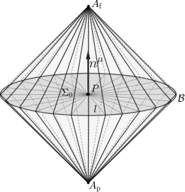
Figure 1: A causal diamond centred in a flat spacetime point $P$. We suppress $D-3$ angular coordinates. The unit, future-directed timelike vector $n^{\mu}$ defines the local direction of time. The diamond’s base is a $\left(D-1\right)$-dimensional spacelike ball $\Sigma_{0}$ centred in $P$ and of radius $l$. Its boundary $\mathcal{B}$ is an approximate $\left(D-2\right)$-sphere. The null generators of the diamond’s boundary are depicted by lines starting in the diamond’s past apex $A_{\text{p}}$ ($t=-l$) and ending in the future apex $A_{\text{f}}$ ($t=l$). The ball $\Sigma_{0}$ lies at the intersection of a future light cone starting in $A_{\text{p}}$ and a past light cone ending in $A_{\text{f}}$.

The particulars of the construction of an LCD are not relevant for our conclusions (as we asserted in the introduction, they do follow from the basic requirements of a horizon entropy proportional to the area, which we introduce in detail in subsection II.3, and the strong equivalence principle, which we discuss in section IV). We simply need a locally constructed causal horizon whose spatial cross-section is an approximate sphere. That being said, two definitions of LCDs are especially well suited for derivations of the gravitational dynamics we study in section V. In the following, we briefly introduce both constructions, focusing on their features relevant for our purposes, and explain their use.

Light-cone cut LCD.

The first type of LCD we work with is a light-cone cut LCD [47]. To construct it we begin at a point $A_{\text{p}}$, the past apex of the eventual diamond (see figure 1). We fix the unit timelike vector $n^{\mu}$ as the local direction of time and take the future directed null vector fields $k_{-}^{\mu}$ at $A_{\text{p}}$ normalised so that $n_{\mu}k_{-}^{\mu}=-1$. We then construct the past boundary of the LCD as a congruence of null wordlines tangent to $k_{-}^{\mu}$. The spacelike cross-section of this congruence at the affine parameter length $l$ measured along $k_{-}^{\mu}$ corresponds to an approximate $\left(D-2\right)$-sphere $\mathcal{B}$, whose interior, an approximate $\left(D-1\right)$-dimensional spacelike ball $\Sigma_{0}$, is the base of the light-cone cut LCD. We call the centre of the ball $P$.

The construction of the future (contracting) part of the light-cone cut LCD is, as mentioned above, not needed to be fixed for our purposes. The most straightforward option would be to specify the future-directed null vector fields $k_{+}^{\mu}$ on $\mathcal{B}$. We can define them so that $n_{\mu}k_{+}^{\mu}=-1$ and, denoting the projection of $k_{-}^{\mu}$ on the surface orthogonal to $n^{\mu}$ by $m^{\mu}$, the same projection of $k_{+}^{\mu}$ is $-m^{\mu}$. In other words, we choose the congruence with a negative expansion. Then, the congruence of the null wordlines tangent to $k_{+}^{\mu}$ forms the future boundary of the causal diamond.

The light-cone cut LCD is well adapted for a physical process approach to deriving the gravitational dynamics from thermodynamics. It is based on tracking the matter flux across the local causal horizon and the corresponding changes in entropy. A thermodynamic equilibrium condition imposed on these entropy changes then encodes the equations governing gravitational dynamics [17, 22, 15, 34]. We carry out a variant of a physical process approach derivation in subsection V.1. To evaluate the changes in entropy in this approach, we need to fully specify the geometry of one suitable slice of the LCD’s past null boundary. At the same time, we do not require to completely fix the geometry of the spatial slices or the entire structure of the diamond (in particular, the details of the future null boundary of the LCD are unimportant for our purposes). The light-cone cut construction indeed fully specifies the past null boundary of the LCD, as needed for the physical process approach.

Geodesic LCD.

The second definition we consider is a geodesic LCD [43, 47]. To construct it, we choose a regular spacetime point $P$ and a local direction of time $n^{\mu}$. Next, we send out geodesics of affine length $l$ in every direction orthogonal to $n^{\mu}$. Given that $l$ is much smaller than the curvature length scale, these geodesics do not intersect and form a spacelike $\left(D-1\right)$-dimensional geodesic ball $\Sigma_{0}$, whose boundary is an approximate $\left(D-2\right)$-sphere $\mathcal{B}$. The geodesic LCD then corresponds to the union of the past and future Cauchy developments of $\Sigma_{0}$ (its domain of dependence).

This construction of an LCD is perfectly suited for the equilibrium approach to deriving the gravitational dynamics we discuss in subsection V.2. Its starting point is an LCD in equilibrium. Then, one introduces a small, simultaneous perturbation of both the spacetime geometry and the matter fields. Since the perturbation is considered away from an equilibrium configuration, the corresponding perturbation of the total entropy vanishes to the leading order. This condition encodes the equations governing gravitational dynamics [43, 14, 16]. In this case, rather than studying evolution of the null boundary, one needs to evaluate the perturbation of the matter fields (and the corresponding entropy) inside a spatial slice of the LCD. Therefore, we need to fully fix the geometry of a spatial slice in which lies the LCD’s centre $P$, while we can allow ambiguities in the definition of the LCD’s boundary. The geodesic LCD construction indeed completely fixes the geodesic ball $\Sigma_{0}$. Therefore, it is ideally suited for deriving the equations governing gravitational dynamics from a small perturbation of the geometry of $\Sigma_{0}$ and the matter fields contained within it.

Conformal isometry of LCDs.

For either construction of an LCD, we can conveniently expand the metric using Riemann normal coordinates [48]. With that aim, we choose $P$ as the origin and specify the local time coordinate $t$ so that $n^{\mu}=\left(\partial_{t}\right)^{\mu}$. Then, we similarly choose $D-1$ spacelike directions to specify the spatial coordinates. We determine the coordinates of any point by the affine parameter of a geodesic connecting it with the origin $P$, such a geodesic being unique on distances much smaller than the local curvature length scale. The Riemann normal coordinate expansion of the metric around $P$ then reads

$$g_{\mu\nu}(x)=\eta_{\mu\nu}-\frac{1}{3}R_{\mu\alpha\nu\beta}\left(P\right)x^{\alpha}x^{\beta}+O\left(x^{3}\right),$$ (1)

where $\eta_{\mu\nu}$ denotes the flat spacetime metric. The Christoffel symbols by construction vanish at $P$ and obey

$$\Gamma^{\mu}_{\rho\sigma}\left(x\right)=-\frac{2}{3}R^{\mu}_{\;\>(\rho\sigma)\nu}\left(P\right)x^{\nu}+O\left(x^{2}\right).$$ (2)

Causal diamonds in flat spacetime are formed by an intersection of light cones, whose shape is invariant under scaling transformations of the metric. Consequently, there exists a conformal isometry of the causal diamond, generated by a conformal Killing vector. For LCDs in a curved spacetime, this isometry is only approximate (up to $O\left(l^{3}\right)$ curvature-dependent corrections) and the conformal Killing vector generating it reads

$$\zeta^{\mu}=C\left[\left(l^{2}-t^{2}-r^{2}\right)\left(\partial_{t}\right)^{\mu}-2rt\left(\partial_{r}\right)^{\mu}\right],$$ (3)

where $r$ stands for the radial geodesic distance from point $P$, $t$ is the time coordinate measured along vector $n^{\mu}$, and $C$ denotes an arbitrary constant determining the normalisation of $\zeta^{\mu}$. The conformal Killing vector $\zeta^{\mu}$ is null on the boundary of the LCD and vanishes at $\mathcal{B}$. Thence, the LCD’s null boundary represents a bifurcate conformal Killing horizon and the $\left(D-2\right)$-sphere $\mathcal{B}$ its bifurcation surface.

II.2 Temperature

Upon discussing the geometry of LCDs, we turn to their thermodynamics. The key ingredient is of course a notion of temperature. There exist several distinct proposals for assigning a temperature to LCDs [3, 49, 50, 51, 52]. These proposals have not been associated with a detector response and their physical interpretation remains unclear. However, to derive the equations governing gravitational dynamics from thermodynamics, we do not actually need a temperature of an LCD. We only require a temperature associated with some suitable class of observers moving inside the causal diamond. In this case, the finite-time Unruh effect provides a robust, detector-based notion of temperature for observers moving inside an LCD with sufficiently large constant accelerations [53, 54, 55, 56]. This temperature can be straightforwardly applied in thermodynamics of LCDs [54, 16]. Nevertheless, since the literature on thermodynamics of spacetime rarely compares the different temperatures associated with LCDs, we find it of interest to first briefly review the proposals for assigning a temperature to an LCD (rather than to a particular observer).

Surface gravity proposal.

The first proposal uses the presence of the conformal Killing horizon associated with the conformal Killing vector $\zeta^{\mu}$ given in equation (3) and suggests that, much like the Killing horizons of black holes, it possesses a temperature proportional to its surface gravity [3], i.e.,

$$T_{\kappa}=\frac{\hbar\kappa}{2\pi}=\frac{\hbar lC}{\pi},$$ (4)

where $C$ is an arbitrary constant that corresponds to the normalisation of $\zeta^{\mu}$. Several particular choices of $C$ have been previously advocated in the literature [43, 3, 16], but they lack a clear physical motivation. In particular, setting $C=1/l^{2}$ makes $\zeta^{\mu}$ coincide with the velocity of the inertial observer in the LCD’s origin $P$. For any $C>1/l^{2}$, we may always find a constantly accelerating observer inside the LCD whose velocity coincides with $\zeta^{\mu}$ at some point. The limit $C\to\infty$ is equivalent to the limit $a\to\infty$. Values $C<1/l^{2}$ do not have a clear interpretation in terms of observer velocities. It seems tempting to interpret the temperatures $T_{\kappa}$ corresponding to different values of $C$ as the Unruh temperatures measured by the various accelerating observers. However, an analysis of the finite-time Unruh effect we briefly comment on next suggests that this is the case only for the values of the surface gravity such that $\kappa\gg 1/l$, i.e., $C\gg 1/l^{2}$.

Finite-time Unruh effect.

Let us consider a uniformly accelerating observer equipped with an Unruh-de Witt detector who moves inside the LCD in the (local approximate) Minkowski vacuum. In the case of an exact Minkowski vacuum observed by an eternally uniformly accelerating observer, the detector measures a thermal bath of particles at the Unruh temperature $T_{\text{U}}=\hbar a/2\pi$ [57, 58, 59], where $a$ is the acceleration. However, in our case, the vacuum is only approximate due to curvature effects and the observer only accelerates for a finite time comparable with the LCD’s size parameter $l$. The Unruh effect under such conditions has been analysed in the literature: the detector still perceives a state well approximated by a thermal bath of particles at the Unruh temperature $T_{\text{U}}=\hbar a/2\pi$, provided that the acceleration $a$ is sufficiently large [53, 55, 56]. More precisely, we must have $a\gg 1/l$ (since $l$ is already chosen to be much smaller than the local curvature length scale, this is the only condition we must satisfy). One further requires that the detector’s energy gap $\Omega$ satisfies $\Omega/a\gg 1$ and $\Omega l\ll 1$ [53, 55, 56].

While the expression for the (surface-gravity-dependent) temperature $T_{\kappa}$ in principle makes sense for any constantly accelerating observer inside the LCD (with different normalisations of the conformal Killing vector), we can apparently obtain a detector-based definition of the Unruh temperature only for the observers with sufficiently large accelerations.

II.3 Vacuum entropy of a local causal diamond

A finite lifetime observer whose existence starts in the past apex $A_{\text{p}}$ of the LCD and ends in its future apex $A_{\text{f}}$ perceives the null boundary of the LCD as a causal horizon. Thence, it should be possible to assign entropy to this observer, quantifying their lack of information about the exterior region. Several approaches to computing entropy of a horizon indeed support the idea that local causal horizons (associated with a class of observers that perceive them) possess finite entropy [19, 20, 2, 21, 60, 3, 61, 62].

In particular, there exists an established way to introduce entropy of a local causal horizon independently of the gravitational action. The Reeh-Schlieder theorem [63] for quantum field theory in flat spacetime implies the existence of vacuum quantum entanglement between the interior and the exterior region of the LCD. Consequently, an observer restricted to the interior of the LCD measures a non-zero entanglement entropy [19, 20, 21]. Detailed calculations [19, 20] show that this entropy diverges unless one introduces a suitable ultraviolet cutoff corresponding to a length scale $\varepsilon$. Upon introducing a cutoff, the entanglement entropy becomes finite and proportional to the horizon area $\mathcal{A}$, i.e., $S_{\text{e}}=\eta\mathcal{A}$ [19, 20, 21]. The proportionality constant $\eta$ scales with the inverse square of the cutoff length, $\eta\propto 1/\varepsilon^{2}$, and its value further depends on the matter fields present in the spacetime. If we take $\varepsilon$ to be of the order of the Planck length, $l_{\text{P}}$, the entanglement entropy of any causal horizon (including that of an LCD) becomes comparable with Bekenstein entropy, $S_{\text{B}}=\mathcal{A}/\left(4\hbar G\right)$. For this reason, quantum entanglement has also been suggested as a possible microscopic explanation of black hole entropy [19, 20]. An important feature of entanglement entropy is that it has (to leading order) the same areal density for any boundary [21]. This outcome agrees with the results one obtains from the standard (gravitational action-dependent) approaches to computing entropy associated with a horizon [1, 4, 62]. However, some criticisms to the entanglement interpretation of horizon entropy has been put forward [64, 21, 65]:

• Entanglement entropy depends on which quantum fields are present in the spacetime. This criticism can be addressed in approaches that make the cutoff $\varepsilon$ (or the Planck length) also sensitive to the matter content of the theory, making the entanglement entropy independent of it [66, 67, 21].

• The choice of Planck length as the ultraviolet cutoff can be motivated [44, 45, 46], but it lacks a clear justification. Furthermore, the cutoff breaks the local Lorentz invariance of the theory. However, the calculation has also been rephrased using a covariant Pauli-Villars regulator, confirming the previously obtained cutoff-dependent results [66].

• It has been argued that, if the entanglement entropy explains the leading order term in black hole entropy, the vacuum fluctuations also significantly change black hole energy, breaking the self-consistency of the approach [68, 69, 64]. However, arguments against this viewpoint have been presented as well [66, 67, 70, 71].

• Many approaches to quantum gravity introduce some discretisation of the spacetime, which only allows a finite subregion of it to have finitely many degrees of freedom. However, the Reeh-Schlieder theorem, which provides the theoretical justification of quantum entanglement between arbitrary spacelike separated subregions, only works for systems with infinitely many degrees of freedom. For systems with finitely many degrees of freedoms, it appears that quantum entanglement does not generically occur [65]. This observation undermines the entanglement interpretation of Bekenstein entropy assuming that spacetime is discretised. We are not aware of any way to refute this objection.

Although the entanglement interpretation of horizon entropy is often invoked in derivations of gravitational dynamics from thermodynamics, the derivation does not depend on the entropy interpretation in any way. All that one really needs to assume is the following. The observers perceiving a local causal horizon cannot access its exterior and should measure some entropy quantifying this fact. It should be possible to express this entropy in terms of the properties of the boundary, as it represents the only feature of the exterior accessible to the interior observer. Then, following the logic of the original proposal for black hole entropy [18], we find entropy proportional to the horizon area to the leading order, $S=\eta\mathcal{A}$, to be the simplest possibility. We do not have to make any assumptions about the microscopic origin of this entropy. Moreover, we do not need to fix the proportionality constant $\eta$. The strong equivalence principle guarantees that $\eta$ is a universal constant. If that were not the case, one could devise a local experiment measuring the entropy density and obtain different results in two distinct locations, falsifying the statement of the principle. Then, rather than fixing $\eta$ to a specific value, we may instead define the Newton gravitational constant in terms of $\eta$ [43]. Since we are deriving the gravitational dynamics from thermodynamics and not the other way around, we find this approach sensible regardless of whether gravity is a fundamental interaction or not.

As an aside, if one specifies the gravitational dynamics a priori, a number of standard approaches show that LCDs indeed possess entropy proportional to its area to the leading order:

• Wald entropy density [4, 5] has the same form for both a black hole Killing horizon and for a conformal Killing horizon of an LCD (both for Diff-invariant [3] and for WTDiff-invariant [8, 9] theories of gravity). The entropy prescription follows from evaluating the Hamiltonian corresponding to evolution along the conformal Killing vector $\zeta^{\mu}$ for the interior of the LCD at $t=0$ (the spatial ball $\Sigma_{0}$).

• Entropy of an LCD can be computed via the Cardy formula [74] as the symmetries of a wide class of null surfaces (including black hole horizons and local causal horizons) form a Virasoro algebra with a central charge, that is identical to the algebra of symmetries of a $2$-dimensional conformal field theory [75, 60]. The Cardy formula valid for such a theory then allows us to compute the entropy from the central charge. It again yields the same entropy prescription for any causal horizon.

• A Euclidean canonical ensemble has been constructed for LCDs [61, 62]. The method obtains the canonical partition function as a Euclidean path integral of the gravitational action in flat spacetime under the assumption of fixed volume of the spatial ball $\Sigma_{0}$ (implemented via a Lagrange multiplier). The resulting expression for entropy has again the same form as for a black hole.

Naturally, all the entropy calculations we have just listed rely on the knowledge of the gravitational action. Then, while they serve as supporting arguments for assigning entropy to LCDs, invoking them to derive the gravitational dynamics from thermodynamics clearly leads to a circular argument. We stress that the derivations we present in section V do not in any way rely on these approaches to compute entropy. We only list them here to provide a broader context.

II.4 Entropy of matter

We now have expressions for the temperature associated with an LCD and for entropy associated with its horizon. The last ingredient necessary to complete the thermodynamic description is entropy of the matter fields contained in the LCD. This entropy can be defined in several different ways. To recover the gravitational dynamics, we require an entropy definition compatible with the Einstein equivalence principle, i.e., one that is local and Lorentz invariant. These requirements fix the matter Hamiltonian to be (roughly speaking) a volume integral of the time-time component of the energy-momentum tensor. Then, the entropy of matter fields (regardless of its precise definition) is also linear in the energy-momentum tensor. If the LCD is in equilibrium, the net change of its entropy must vanish. Therefore, a change in matter entropy is compensated by a corresponding change in the horizon entropy, proportional to its area. Since the change of the horizon area is linear in the Ricci tensor [17, 43], this equilibrium condition connect the energy-momentum tensor with the Ricci tensor and encodes the equations governing the gravitational dynamics.

We focus on two particular definitions of matter entropy which we use for the gravitational dynamic derivations in section V: the (semi)classical entropy flux across the LCD’s horizon and the quantum von Neumann entropy of the matter contained in the spatial ball $\Sigma_{0}$. The (semi)classical definition has the advantage of being rather intuitive and also of tracking the entropy flux across the horizon, making it ideally suited for the physical process derivation of the equations governing the gravitational dynamics we study in subsection V.1. The von Neumann definition is non-local for completely general matter fields and we cannot straightforwardly compute the entropy flux in this case. However, as von Neumann entropy deals with quantum matter fields, it allows one to study the semiclassical gravitational dynamics, i.e., the regime of classical spacetime curvature being sourced by quantum expectation value of the energy-momentum tensor. We work with von Neumann entropy in the equilibrium approach in subsection V.2.

In the following, we briefly introduce both definitions. We work in a generic curved spacetime. However, we use that the LCD’s size parameter $l$ is much smaller than the curvature length scale and we treat the spacetime as being approximately flat inside the LCD.

Clausius entropy flux.

Following the analysis carried out for generic bifurcate null surfaces [54], we recall the construction of a (semi)classical matter entropy flux across the null boundary of the LCD. We start with the classical energy flux across an arbitrary timelike $\left(D-1\right)$-dimensional surface $\mathcal{S}$

$$\Delta Q=-\int_{\mathcal{S}}T_{\mu\nu}V^{\nu}N^{\mu}\text{d}^{D-1}\mathcal{S},$$ (5)

where $V^{\nu}$ denotes the future-directed unit timelike vector tangent to $\mathcal{S}$ and $N^{\mu}$ the outward-poiting spacelike unit normal to it. We interpret equation (5) as the heat flux $\Delta Q$ [17, 22, 54].

In particular, we consider the heat flux across a timelike surface $\mathcal{S}$ formed by a congruence of wordlines of uniformly accelerating observers moving inside the LCD. The proper time $\tau$ of the uniformly accelerating observers can be expressed in terms of the inertial, coordinate time $t$ measured along the vector $n^{\mu}$

$$\text{d}t=\cosh\left(a\tau\right)\text{d}\tau,$$ (6)

where $a$ denotes the observer’s acceleration. The tangent vector $V^{\nu}$ and the normal $N^{\mu}$ in this case obey

$$V^{\mu} =\left(\cosh\left(a\tau\right),-\sinh\left(a\tau\right),0,\dots\right)$$ (7)

$$N^{\mu} =\left(-\sinh\left(a\tau\right),\cosh\left(a\tau\right),0,\dots\right).$$ (8)

We evaluate the heat flux for a slice of $\mathcal{S}$ extended between the past apex of the LCD ($t=-l$) and some time $t\leq 0$ (as we focus only on the past boundary of the causal diamond in section V, but a generalisation to positive times is straightforward). In the limit $a\to\infty$, the surface $\mathcal{S}$ approaches the causal horizon $\mathcal{H}$ of the LCD. For large accelerations, the heat flux (5) reads

$$\Delta Q=\int_{-\infty}^{\tau\left(t\right)}\text{d}\tau\int\text{d}^{D-2}\mathcal{A}\left(T_{tt}+T_{rr}-2T_{tr}\right)e^{2a\tau}+O\left(a^{0}\right),$$ (9)

where $O\left(a^{0}\right)$ denotes the terms finite in the limit $a\to\infty$. One can notice that the components of the energy-momentum tensor in the integrand correspond to an invariant expression $T_{\mu\nu}k_{-}^{\mu}k_{-}^{\nu}$, where $k_{-}^{\mu}=\left(1,1,0,\dots\right)$ is the future pointing null vector tangent to the past boundary of the causal diamond (which the timelike surface $\mathcal{S}$ approaches for large accelerations). Changing the integration variable in equation (9) from the proper time $\tau$ to the coordinate time $t$ then yields

$$\Delta Q=\int_{-l}^{t}\text{d}t^{\prime}\int\text{d}^{D-2}\mathcal{A}\,at^{\prime}T_{\mu\nu}k_{-}^{\mu}k_{-}^{\nu}+O\left(a^{0}\right).$$ (10)

The first term is linear in $a$ and becomes infinite as the timelike surface $\mathcal{S}$ approaches the null boundary $\mathcal{H}$ of the LCD. Thence, to define a finite entropy flux across $\mathcal{H}$ by the Clausius equilibrium prescription $\Delta S_{\text{C}}=\Delta Q/T$, where $T$ denotes the temperature, we must consider a notion of temperature that also diverges at the same rate. We can consider the Unruh effect, which ensures that the uniformly accelerating observer perceives a heat bath of temperature $T_{\text{U}}=\hbar a/\left(2\pi\right)$ (provided that $a\gg 1/l$, see subsection II.2 for details). Then, the Clausius entropy flux given by the relation $\Delta S_{\text{C}}=\Delta Q/T_{\text{U}}$ (using that $T_{\text{U}}$ is approximately constant) is indeed finite in the limit of $a\to\infty$, i.e., for horizon $\mathcal{H}$.

For our purposes, it turns out to be more useful to evaluate here the time derivative of the Clausius entropy, $\text{d}S_{\text{C}}\left(t\right)/\text{d}t$ at a constant coordinate time $t$. Differentiating equation (10) with respect to $t$, dividing by the Unruh temperature $T_{\text{U}}$, and taking the limit $a\to\infty$ then yields [54]

$$\frac{\text{d}S_{\text{C}}\left(t\right)}{\text{d}t}=\frac{2\pi}{\hbar}tT_{\mu\nu}\left(P\right)\int_{\mathcal{B}_{t}}k_{-}^{\mu}k_{-}^{\nu}\text{d}^{D-2}\mathcal{A}+O\left(l^{D+2}\right),$$ (11)

where $\mathcal{B}_{t}$ is a spatial cross-section of $\Sigma$ at time $t$. Equation (11) applies to any LCD, whose size parameter $l$ is much smaller than the local curvature length scale. The smallness of $l$ has also allowed us to approximate the energy-momentum tensor by its value in the LCD’s origin $P$. Equation (11) is semiclassical in the sense that it describes the heat flux classically, but involves the Unruh temperature which is of quantum origin.

Von Neumann entropy.

Rather than tracking the entropy flux across the horizon, we can also compute the total von Neumann entropy of the matter in the spatial ball $\Sigma_{0}$ at time $t=0$. Due to local Lorentz invariance, the thermal density operator corresponding to the surface gravity-dependent temperature $T_{\kappa}=\hbar\kappa/\left(2\pi\right)$ (see equation (4)) in the $\left(D-1\right)$-dimensional spatial ball $\Sigma_{0}$ reads $\rho_{\kappa}=e^{-K/T_{\kappa}}/\text{Tr}\left(e^{-K/T_{\kappa}}\right)$; the operator $K$ is referred to as the modular Hamiltonian and corresponds to the boost generator [58, 43, 42]. In general, the modular Hamiltonian $K$ can be a complicated non-local operator. However, for conformally invariant matter fields, it corresponds to the following integral over $\Sigma_{0}$ [58, 43, 42]

$$K=\int_{\Sigma_{0}}T^{\mu\nu}\zeta_{\mu}n_{\nu}\text{d}^{D-1}\Sigma.$$ (12)

To compute von Neumann entropy of the matter fields, we can now apply the von Neumann formula $S_{\text{vN}}=-\text{Tr}\left(\rho\ln\rho\right)$ to the density operator $\rho_{\kappa}$. For a small perturbation of the density matrix $\delta\rho$, a direct calculations yields for the corresponding change of von Neumann entropy

$$\delta S_{\text{vN}}=\frac{1}{T_{\kappa}}\text{Tr}\left(\delta\rho K\right)=\frac{1}{T_{\kappa}}\langle K\rangle_{\delta\rho}\equiv\frac{1}{T_{\kappa}}\delta\langle K\rangle.$$ (13)

In particular, for conformally invariant matter fields equation (12) implies

$$\delta S_{\text{vN,CFT}}=\frac{2\pi}{\kappa}\int_{\Sigma_{0}}\delta\langle T^{\mu\nu}\rangle\zeta_{\mu}n_{\nu}\text{d}^{D-1}\Sigma+O\left(l^{D+2}\right).$$ (14)

The $O\left(l^{D+2}\right)$ terms represent the curvature-dependent corrections that can be neglected for a small enough LCD.

A similar general expression for entropy cannot be derived for non-conformal matter fields. Nevertheless, for a theory that possesses a fixed ultraviolet point (around which it is approximately conformal) a generalisation of equation (14) has been proposed [43] and verified for a class of such theories [41, 40]. It reads

$$\delta S_{\text{vN}}=\delta S_{\text{vN,CFT}}+\delta X,$$ (15)

where new term $\delta X$, is a rather complicated, but explicitly known, spacetime scalar that is a function of the LCD’s size parameter $l$. Equation (15) holds only if $l$ is much smaller than the relevant length scales of the quantum field theory (such as the Compton lengths). Otherwise, its derivation fails [43, 41, 40].

Although the Clausius entropy flux (11) and the matter von Neumann entropy (15) are conceptually very different, it has been shown that both entropy definitions lead to equivalent gravitational dynamics [16, 34, 35]. Moreover, for conformally invariant matter fields, we can explicitly show that both entropies are equivalent [34].

III Overview of Weyl transverse gravity and its generalisations

The main aim of this paper is to discuss how thermodynamic arguments naturally lead to Weyl transverse gravity. To provide the necessary context for this discussion, we now briefly review this theory.

First of all, to construct any WTDiff-invariant theory of gravity, one needs to introduce a non-dynamical volume $D$-form, $\bm{\omega}=\omega\left(x\right)\text{d}x^{0}\wedge\text{d}x^{1}\wedge...\wedge\text{d}x^{D-1}$, where $\omega$ is a strictly positive function [76, 32]. In principle, it is possible to construct WTDiff-invariant gravitational theories by introducing dynamics for the volume $D$-form $\bm{\omega}$ [77], but we do not explore this option here any further.

To simplify the notation, we define an auxiliary, WTDiff-invariant metric constructed from the dynamical metric $g_{\mu\nu}$ and the background volume measure $\omega$,

$$\tilde{g}_{\mu\nu}=\left(\sqrt{-\mathfrak{g}}/\omega\right)^{-2/D}g_{\mu\nu},$$ (16)

where $\mathfrak{g}$ denotes the metric determinant. Both $\sqrt{-\mathfrak{g}}$ and $\omega$ are scalar densities of weight $+1$, ensuring that $\tilde{g}_{\mu\nu}$ (which depends on their ratio) is a tensor. This auxiliary metric can be understood as a restriction of $g_{\mu\nu}$ to the unimodular gauge, $\sqrt{-\mathfrak{g}}=\omega$. We stress that we treat $\tilde{g}_{\mu\nu}$ as a mere notational device, keeping $g_{\mu\nu}$ as the dynamical field. To ensure we always work with WTDiff-invariant expressions, raising and lowering of indices is performed with $\tilde{g}_{\mu\nu}$ and the inverse metric $\tilde{g}^{\mu\nu}$.

The Levi-Civita connection defined with respect to $\tilde{g}_{\mu\nu}$ (the Weyl connection) reads

$$\tilde{\Gamma}^{\mu}_{\;\>\nu\rho}=\Gamma^{\mu}_{\;\>\nu\rho}-\frac{1}{D}\left(\delta^{\mu}_{\nu}\delta^{\lambda}_{\rho}+\delta^{\mu}_{\rho}\delta^{\lambda}_{\nu}-g_{\nu\rho}g^{\lambda\mu}\right)\partial_{\lambda}\ln\frac{\sqrt{-\mathfrak{g}}}{\omega},$$ (17)

where $\Gamma^{\mu}_{\;\>\nu\rho}$ denotes the Levi-Civita connection with respect to the dynamical metric, $g_{\mu\nu}$. Using the Weyl connection, we introduce an auxiliary, WTDiff-invariant Riemann tensor

$$\tilde{R}^{\mu}_{\;\>\nu\rho\sigma}=2\tilde{\Gamma}^{\mu}_{\;\>\nu[\sigma,\rho]}+2\tilde{\Gamma}^{\mu}_{\;\>\lambda[\rho}\tilde{\Gamma}^{\lambda}_{\;\>\sigma]\nu}.$$ (18)

III.1 Weyl transverse gravity

The simplest action one can construct from the auxiliary metric and the corresponding Riemann tensor is that of Weyl transverse gravity, i.e.,

$$I_{\text{WTG}}=\frac{1}{16\pi G}\int_{\text{V}}\tilde{R}\omega\text{d}^{D}x,$$ (19)

where V is the domain of integration and $\tilde{R}=\tilde{g}^{\mu\nu}\tilde{R}_{\mu\nu}$ denotes the scalar curvature defined with respect to $\tilde{g}_{\mu\nu}$. By construction, $I_{\text{WTG}}$ is invariant under Weyl transformations,

$$\delta g_{\mu\nu}=e^{2\sigma}g_{\mu\nu},$$ (20)

where $\sigma$ is an arbitrary scalar function. The volume measure $\omega$ is by definition unaffected by Weyl transformations, ensuring the Weyl invariance of $\tilde{g}_{\mu\nu}$. Furthermore, $I_{\text{WTG}}$ is invariant under transverse diffeomorphisms but not under longitudinal ones. However, we must be careful to consider the appropriate notion of transversality. The usual condition on the generator $\xi^{\mu}$ of transverse diffeomorphisms, $\nabla_{\mu}\xi^{\mu}=0$, is not Weyl invariant. Thus, it cannot be satisfied in every Weyl frame simultaneously, making it unsuitable for Weyl transverse gravity. Instead, one must define transversality with respect to the Weyl invariant covariant derivative. Hence, the appropriate transversality condition reads

$$\tilde{\nabla}_{\mu}\xi^{\mu}=0\qquad\iff\qquad\nabla_{\mu}\xi^{\mu}=\xi^{\mu}\partial_{\mu}\ln\frac{\sqrt{-\mathfrak{g}}}{\omega}.$$ (21)

Since the Lie derivative of the volume $D$-form $\bm{\omega}$ yields $\pounds_{\xi}\bm{\omega}=\bm{\omega}\tilde{\nabla}_{\mu}\xi^{\mu}$ (this result can be obtained by direct computation and also follows from the fact that $\tilde{\nabla}_{\mu}\bm{\omega}=0$), we can understand the transversality condition as defining the volume preserving transformations. Transverse diffeomorphisms transform the dynamical metric in the usual way

$$\delta_{\xi}g_{\mu\nu}=2\nabla_{(\nu}\xi_{\mu)}.$$ (22)

Since the spacetime volume measure is nondynamical, adding any constant term to the Weyl transverse gravity Lagrangian corresponds simply to shifting the action by a constant and does not affect dynamics in any way. Hence, we are free to set this constant term to zero in the following. This marks a departure from general relativity, where a constant term in the Lagrangian corresponds to the cosmological constant.

III.2 Coupling to matter

Let us now discuss coupling Weyl transverse gravity to matter. The action for a matter field minimally coupled to WTDiff-invariant gravity may be written as

$$I_{\psi}=\int_{\text{V}}L_{\psi}\omega\text{d}^{D}x,$$ (23)

where $L_{\psi}$ is some scalar function of matter variables, $\psi$, their partial derivatives and the auxiliary metric, $\tilde{g}_{\mu\nu}$. The matter variables are by definition unaffected by Weyl transformations, guaranteeing the overall Weyl invariance of $I_{\psi}$. If more than one minimally coupled matter field is present, the action is simply a sum of several terms of the above stated form.

To find equations of motion for Weyl transverse gravity, we vary the gravitational and matter action with respect to the dynamical metric $g^{\mu\nu}$, obtaining traceless, WTDiff-invariant equations of motion

$$\tilde{R}_{\mu\nu}-\frac{1}{D}\tilde{R}\tilde{g}_{\mu\nu}=8\pi G\left(\tilde{T}_{\mu\nu}-\frac{1}{D}\tilde{T}\tilde{g}_{\mu\nu}\right),$$ (24)

where we define

$$\tilde{T}_{\mu\nu}=-2\frac{\partial L_{\psi}}{\partial\tilde{g}^{\mu\nu}}+L_{\psi}\tilde{g}_{\mu\nu}.$$ (25)

Whereas Diff invariance of gravitational dynamics yields the local energy-momentum conservation condition, $\nabla_{\nu}T_{\mu}^{\;\>\nu}=0$, this is not in general true for WTDiff-invariant theories. Nevertheless, WTDiff invariance of the matter action does imply a weaker condition [78]

$$\tilde{\nabla}_{\nu}\tilde{T}_{\mu}^{\;\>\nu}=\tilde{\nabla}_{\mu}\mathcal{J},$$ (26)

where $\mathcal{J}$ is a scalar function. It is easy to see that if $\mathcal{J}\neq 0$, then the energy-momentum tensor is not locally conserved (for a more detailed discussion of local energy-momentum non-conservation see, e.g. [35, 25]). Nonetheless, the tensor

$$\tilde{T}^{\prime}_{\mu\nu}=\tilde{T}_{\mu\nu}-\mathcal{J}\tilde{g}_{\mu\nu},$$ (27)

which will be relevant throughout, is indeed divergenceless.

Now, using the contracted Bianchi identities

$$2\tilde{\nabla}_{\nu}\tilde{R}_{\mu}^{\;\>\nu}=\tilde{\nabla}_{\mu}\tilde{R},$$ (28)

we can rewrite the traceless equations of motion (24) in a divergenceless form of the standard Einstein equations. By taking the divergence of equations (24) and rewriting it with the help of the Bianchi identities (28), we find

$$\tilde{\nabla}_{\mu}\left[\frac{D-2}{2D}\tilde{R}+8\pi G\left(\frac{1}{D}\tilde{T}-\mathcal{J}\right)\right]=0,$$ (29)

where we used equation (26) for the divergence of the energy-momentum tensor. Integrating, we obtain

$$\frac{D-2}{2D}\tilde{R}\tilde{g}_{\mu\nu}+8\pi G\left(\frac{1}{D}\tilde{T}-\mathcal{J}\right)\tilde{g}_{\mu\nu}=\Lambda\tilde{g}_{\mu\nu},$$ (30)

where $\Lambda$ denotes an arbitrary integration constant. Subtracting equation (30) from the traceless equations of motion (24) finally yields

$$\tilde{R}_{\mu\nu}-\frac{1}{2}\tilde{R}\tilde{g}_{\mu\nu}+\Lambda\tilde{g}_{\mu\nu}=8\pi G\tilde{T}^{\prime}_{\mu\nu}.$$ (31)

These equations are of the same form as the Einstein equations with the divergenceless energy-momentum tensor $\tilde{T}^{\prime}_{\mu\nu}$. We can see that the integration constant $\Lambda$ plays the role of the cosmological constant. In contrast with general relativity, $\Lambda$ has no connection with any fixed parameter present in the Lagrangian and is only defined on shell, having in principle different values for the various solutions of the theory. It has been shown that this behaviour of the cosmological constant leads to its radiative stability in the effective field theory treatment of Weyl transverse gravity [76, 32, 25].

III.3 WTDiff-invariant theories of gravity

While we primarily focus on Weyl transverse gravity in the present work, we also show a thermodynamic derivation of equations of motion for a class of more general WTDiff-invariant theories of gravity in section VI. Specifically, we consider arbitrary gravitational Lagrangians constructed from the auxiliary metric and the auxiliary Riemann tensor (but not its derivatives) and restrict our attention to minimally coupled matter fields described by action (23). The most general such action reads

$$I_{\text{WTDiff}}=\int_{\text{V}}L\left(\tilde{g}_{\mu\nu},\tilde{R}^{\mu}_{\;\>\nu\rho\sigma}\right)\omega\text{d}^{D}x+I_{\psi}.$$ (32)

The corresponding traceless equations of motion are [25, 9]

$$\tilde{H}_{\mu\nu}-\frac{1}{D}\tilde{H}\tilde{g}_{\mu\nu}=8\pi G\left(\tilde{T}_{\mu\nu}-\frac{1}{D}\tilde{T}\tilde{g}_{\mu\nu}\right),$$ (33)

where we defined the symmetric tensor

$$\tilde{H}_{\mu\nu}=16\pi G\left[\tilde{E}_{(\nu}^{\;\;\>\lambda\rho\sigma}\tilde{R}_{\mu)\lambda\rho\sigma}-2\tilde{\nabla}_{\rho}\tilde{\nabla}_{\sigma}\tilde{E}_{(\mu\;\;\;\nu)}^{\;\;\>\rho\sigma}\right],$$ (34)

with the tensor $\tilde{E}_{\mu}^{\;\>\nu\rho\sigma}$ being the derivative of the Lagrangian with respect to the auxiliary Riemann tensor

$$\tilde{E}_{\mu}^{\;\>\nu\rho\sigma}=\frac{\partial L}{\partial\tilde{R}^{\mu}_{\;\>\nu\rho\sigma}}.$$ (35)

For the special case of Weyl transverse gravity, $\tilde{H}_{\mu\nu}$ is simply the auxiliary Ricci tensor $\tilde{R}_{\mu\nu}$. In general, $\tilde{H}_{\mu\nu}$ depends on second derivatives of the auxiliary Riemann tensor, coming from the term $-2\tilde{\nabla}_{\rho}\tilde{\nabla}_{\sigma}\tilde{E}_{\mu\;\>\;\>\nu}^{\;\>\rho\sigma}$.

In the same way that Weyl transverse gravity represents a WTDiff-invariant alternative to general relativity, it has been shown that there exists a WTDiff-invariant theory corresponding to any Diff-invariant one [25]. Such pairs of corresponding theories have the same classical dynamics, except for the different behaviour of $\Lambda$. Likewise, for every WTDiff-invariant theory that incorporates local energy-momentum conservation, there exists a Diff-invariant theory equivalent to it in this sense.

IV Equivalence principle(s) and WTDiff-invariant gravity

A key ingredient in any derivation of the equations governing gravitational dynamics from thermodynamics is some version of the equivalence principle because of the following reasons. First, to define the temperature associated with a local causal horizon one uses the Unruh effect, according to which a uniformly accelerating observer sees the Minkowski vacuum as a thermal bath of particles with a temperature proportional to the observer’s acceleration. To apply this result locally in a generic curved spacetime, one needs to construct a local, approximate Minkowski vacuum state. The existence of such a state is ensured by a particular formulation of the equivalence principle, known as the Einstein equivalence principle, which guarantees that non-gravitational physics in any spacetime locally behaves in accord with special relativity. Second, the strong equivalence principle allows us to derive the equations for gravitational dynamics in an arbitrary regular spacetime point and then extend their validity to the entire spacetime. Thence, to connect thermodynamics of spacetime with WTDiff-invariant gravitational dynamics, we first need to clarify the status of the various formulations of the equivalence principle in the WTDiff-invariant setup.

In addition, the equivalence principle historically played an important role as a guiding principle in the development of the general relativity [79], and the validity of its weak formulation is experimentally tested to a high degree [80, 81]. Furthermore, the status of the equivalence principle in quantum physics has attracted considerable attention lately [82, 83, 84, 85]. Lastly, the various formulations of the equivalence principle allow one to classify various theories of gravity. Specifically, while the Einstein equivalence principle applies essentially to any local, Diff-invariant theory, the strong equivalence principle concerning also self-gravitating test particles is only known to be valid in general relativity (in four dimensions). Our most important observation in this section is that Weyl transverse gravity also incorporates the strong equivalence principle. Then, general relativity and Weyl transverse gravity are singled out as the only known gravitational theories compatible with this principle.

We proceed by checking the validity of the relevant formulations of the equivalence principle one by one. The classification of the equivalence principles we adapt follows reference [86].

IV.1 Newton equivalence principle

Before going to the more complicated relativistic setting, we first briefly address the weakest formulation of the equivalence principle, the Newton equivalence principle. It states “In the Newtonian limit, the inertial and gravitational masses of a body are equal” [86]. Since it only deals with the Newtonian limit, it is naturally obeyed by Weyl transverse gravity.

IV.2 Weak equivalence principles

The weak equivalence principle reads “Test particles with negligible self-gravity behave, in a gravitational field, independently of their properties”[86]. By test particle we mean one whose back-reaction on its environment can be disregarded. The negligible self-gravity requirement demands that the object’s size is much larger than the Schwarzschild radius corresponding to its mass. The weak equivalence principle holds if the effects of gravity on the trajectory of a test particle can be fully captured by the connection (locally, disregarding geodesic deviations among its constituents and similar effects), which guarantees the universality of motion in a gravitational field [86].

To analyse the validity of the weak equivalence principle for WTDiff-invariant gravity, we first need to discuss motion in a gravitational field in such theories. The standard, Diff-invariant timelike geodesic equation reads

$$u^{\nu}\nabla_{\nu}u^{\mu}=fu^{\mu},$$ (36)

where $u^{\mu}$ denotes a unit vector tangent to the geodesic and $f=u^{\nu}\nabla_{\nu}\ln\sqrt{|u^{2}|}$ (for an affine parametrisation, we have $f=0$). However, this equation is not invariant under Weyl transformations. In other words, force-free trajectories in one Weyl frame are subjected to a force in a different frame. This behaviour clearly breaks the Weyl invariance of physics necessary for WTDiff-invariant gravity.

To find a geodesic equation tailored to WTDiff-invariant gravity, we turn to one of the standard approaches to derive it in the Diff-invariant case. In particular, for any Diff-invariant theory of gravity, one can straightforwardly derive the geodesic equation for a test particle modelled by a spatially localised perfect fluid energy-momentum tensor. If the fluid is pressureless, the divergenceless condition on the energy-momentum tensor is equivalent to the geodesic equation (36). As expected, the gradient of the fluid’s pressure acts as a force and the particle’s trajectory is no longer a geodesic.

In the WTDiff-invariant case, we consider the following WTDiff-invariant perfect fluid energy-momentum tensor $\tilde{T}_{\mu\nu}=\left(\rho+p\right)\tilde{u}_{\mu}\tilde{u}_{\nu}+p\tilde{g}_{\mu\nu}$, where the unit timelike vector $\tilde{u}^{\mu}$ is now normalised to unity with respect to the auxiliary metric. Thence, we have the following relation between $\tilde{u}^{\mu}$ and $u^{\mu}$ considered in the Diff-invariant geodesic equation

$$\tilde{u}^{\mu}=\left(\sqrt{-\mathfrak{g}}/\omega\right)^{-1/D}u^{\mu}.$$ (37)

The WTDiff-invariant divergence of this energy-momentum tensor obeys equation (26)

$$\tilde{g}^{\lambda\nu}\tilde{\nabla}_{\nu}\tilde{T}_{\lambda\mu}= ~{}\tilde{g}_{\mu\lambda}\tilde{u}^{\lambda}\tilde{\nabla}_{\nu}\left[\left(\rho+p\right)\tilde{u}^{\nu}\right]$$

$$+\tilde{\nabla}_{\mu}p+\left(\rho+p\right)\tilde{u}^{\nu}\tilde{\nabla}_{\nu}\tilde{u}_{\mu}=\tilde{\nabla}_{\mu}\mathcal{J},$$ (38)

where $\mathcal{J}$ is a measure of the local energy-momentum non-conservation. Projecting this equation on the surface orthogonal to $\tilde{u}^{\mu}$ via the projection tensor $\tilde{h}^{\mu\rho}=\tilde{g}^{\mu\rho}+\tilde{u}^{\mu}\tilde{u}^{\rho}$ yields

$$\left(\rho+p\right)\tilde{u}^{\nu}\tilde{\nabla}_{\nu}\tilde{u}^{\rho}=\tilde{h}^{\rho\nu}\tilde{\nabla}_{\nu}\left(\mathcal{J}-p\right).$$ (39)

The left hand side is proportional to the WTDiff-invariant acceleration of the test particle $\tilde{a}^{\rho}=\tilde{u}^{\nu}\tilde{\nabla}_{\nu}\tilde{u}^{\rho}$, whereas the right hand side is the force acting on the particle. Aside from the force sourced by the gradient of the pressure, there is also a new contribution sourced by the gradient of the energy non-conservation measure $\mathcal{J}$. Therefore, a force-free trajectory of a test particle composed of a perfect fluid in WTDiff-invariant geometry is characterised by the condition $\tilde{h}^{\rho\nu}\tilde{\nabla}_{\nu}\left(\mathcal{J}-p\right)=0$ (the equivalent condition in the Diff-invariant case reads $h^{\rho\nu}\nabla_{\nu}p=0$ since the Diff invariance implies $\mathcal{J}=0$). For such a perfect fluid the divergence of the energy-momentum tensor yields the condition $\tilde{u}^{\nu}\tilde{\nabla}_{\nu}\tilde{u}^{\rho}=0$ and the particle consequently follows a timelike geodesic trajectory in any Weyl frame. Therefore, allowing for non-affine parametrisations, the appropriate WTDiff-invariant geodesic equation reads

$$\tilde{u}^{\nu}\tilde{\nabla}_{\nu}\tilde{u}^{\mu}=f\tilde{u}^{\mu},$$ (40)

where $f=\tilde{u}^{\nu}\tilde{\nabla}_{\nu}\ln\sqrt{|\tilde{u}^{2}|}$. It is easy to see that equation (40) yields the required WTDiff-invariant force-free trajectories. With this definition of a geodesic, any local, WTDiff-invariant theory of gravity incorporates the weak equivalence principle.

The geodesic equation (40) has further consequences for WTDiff-invariant gravity. It directly shows that, while the dynamical metric $g_{\mu\nu}$ remains the dynamical variable describing gravity, the metric relevant for describing the spacetime geometry in which matter moves is actually the auxiliary one, $\tilde{g}_{\mu\nu}$. Both metrics differ only in their measure of spacetime volume, which cannot be experimentally accessed by any known method [32, 25]. Thence, using $g_{\mu\nu}$ as the dynamical variable and $\tilde{g}_{\mu\nu}$ as the way to measure distances in the spacetime does not allow us to distinguish WTDiff-invariant gravitational theories from the Diff-invariant ones.

A somewhat more sophisticated argument for the weak equivalence principle relies on the Geroch-Jang theorem [87], which gives a useful way to characterise timelike geodesics. Let us assume that for every neighbourhood $\mathcal{U}$ of a curve $\Gamma$ there exists a tensor $\Theta_{\mu\nu}$ satisfying the following properties: (i) $\Theta_{\mu\nu}$ vanishes everywhere outside $\mathcal{U}$; (ii) $\Theta_{\mu\nu}$ is nonzero somewhere in $\mathcal{U}$; (iii) $\Theta_{\mu\nu}$ has vanishing divergence; and (iv) $\Theta_{\mu\nu}$ satisfies the dominant energy condition, i.e., $\Theta_{\mu\nu}n^{\mu}n^{\nu}\geq 0$ for every timelike vector field $n^{\mu}$ and $\Theta_{\mu\nu}n^{\nu}$ is timelike (or vanishing). Then it follows that $\Gamma$ is a timelike geodesic.

• In Diff-invariant gravity, taking $\Theta_{\mu\nu}$ to be the energy-momentum tensor $T_{\mu\nu}$ of the test particle, the theorem guarantees that the particle follows a timelike geodesic, in accord with the weak equivalence principle, provided that the energy-momentum tensor satisfies the necessary dominant energy condition.

• For WTDiff-invariant theories, one needs to apply the theorem to $\tilde{T}^{\prime}_{\mu\nu}$ (27) whose WTDiff-invariant divergence vanishes as required. Of course, demanding the dominant energy condition for $\tilde{T}^{\prime}_{\mu\nu}$ rather than for $\tilde{T}_{\mu\nu}$ is a stronger requirement. However, equations (31) which are the divergenceless equations for Weyl transverse gravity have $\tilde{T}^{\prime}_{\mu\nu}$ on the right hand side. In other words, it plays the same role as the energy-momentum tensor $T_{\mu\nu}$ in general relativity. Thus, $\tilde{T}^{\prime}_{\mu\nu}$ should be relevant for any application of the energy conditions to WTDiff-invariant gravity, e.g. for the proofs of singularity theorems or for the exclusion of solutions containing closed timelike curves. As an aside, this difference is irrelevant for the null energy conditions, since $\mathcal{J}\tilde{g}_{\mu\nu}\tilde{k}^{\mu}\tilde{k}^{\nu}=0$ for any null vector $\tilde{k}^{\mu}$. With the dominant energy condition satisfied, the Geroch-Jang theorem then ensures the validity of the weak equivalence principle for any local, WTDiff-invariant gravitational theory.

IV.3 Einstein equivalence principle

A stronger condition than the weak equivalence principle is the Einstein equivalence principle, which extends it from the motion of particles to all non-gravitational test physics. It states “Fundamental non-gravitational test physics is not affected, locally and at any point of spacetime, by the presence of a gravitational field” [86]. Since WTDiff-invariant theories of gravity do not change the non-gravitational physics (in particular, Weyl transformations do not act on matter fields), the Einstein equivalence principle applies to WTDiff-invariant gravity in the same way it does to Diff-invariant theories. Nevertheless, it should be noted that the status of the Einstein equivalence principle in Diff-invariant theories already presents a fairly subtle issue. In particular, the principle is limited to “fundamental physics” (so as to exclude, e.g. composite bodies whose behaviour can, even locally, depend on the spacetime curvature [86]). This requirement is rather vague, although it is intuitively clear which cases definitely have to be excluded [86]. The important point is that WTDiff invariance in no way makes the subtleties to the formulation of the Einstein equivalence principle any worse.

IV.4 Gravitational weak equivalence principles

The weak equivalence principle can be also generalised to apply to self-gravitating test particles. The resulting formulation is known as the gravitational weak equivalence principle which asserts “Test particles behave, in a gravitational field and in vacuum, independently of their properties” [86]. Unlike the weak equivalence principle, its version for self-gravitating particles is restricted to vacuum. Otherwise, the intrinsic gravitational field would influence the nearby matter, thus breaking the universality.

A simple criterion for the validity of the gravitational weak equivalence principle utilises the Geroch-Jang theorem [23]. However, rather than applying the theorem just to the energy-momentum tensor of the test particle, it also needs to include the perturbation of the gravitational field caused by the presence of the particle (i.e., the effective energy-momentum of its gravitational field). Moreover, one must keep in mind that the geodesic along which the test particle should move lies in the unperturbed spacetime. Splitting the WTDiff-invariant auxiliary metric into the background part $\tilde{g}_{\mu\nu}$ and the perturbation caused by the test particle, $\tilde{\gamma}_{\mu\nu}$, we may similarly split the equations of motion. In the case of Weyl transverse gravity, we obtain the vacuum divergenceless equations for the background metric

$$\tilde{G}_{\mu\nu}=\Lambda\tilde{g}_{\mu\nu},$$ (41)

and the equations governing the perturbation

$$\tilde{\mathcal{G}}_{\mu\nu}+\Lambda\tilde{\gamma}_{\mu\nu}=8\pi G\left(\tilde{T}^{\prime}_{\mu\nu}-\tilde{T}^{\text{(g)}}_{\mu\nu}\right)\equiv 8\pi G\tilde{\mathcal{T}}_{\mu\nu},$$ (42)

where $\tilde{\mathcal{G}}_{\mu\nu}$ denotes the perturbation of the WTDiff-invariant auxiliary Einstein tensor. The first term on the right hand side $\tilde{T}^{\prime}_{\mu\nu}$ corresponds to the divergenceless energy-momentum tensor of the test particle. The second term $\tilde{T}^{\text{(g)}}_{\mu\nu}$ quantifies the effective (WTDiff-invariant) energy-momentum of the gravitational field, which is quadratic in the auxiliary metric perturbation $\tilde{\gamma}_{\mu\nu}$. The tensor $\tilde{\mathcal{T}}_{\mu\nu}$ then quantifies both the energy-momentum of the test particle and its gravitational self-energy.

The tensor $\tilde{\mathcal{T}}_{\mu\nu}$ satisfies the conditions of the Geroch-Jang theorem with respect to the background (unperturbed) metric. Indeed, conditions (i) and (ii) concerning the localisation of the tensor are trivial. Validity of the dominant energy condition (condition (iv)) represents a nontrivial assumption, but it is satisfied for “reasonable” test particles [23]. Lastly, we must check condition (iii), i.e., that $\tilde{\nabla}_{\nu}\tilde{\mathcal{T}}_{\mu}^{\;\>\nu}=0$, where the covariant derivative $\tilde{\nabla}_{\nu}$ is defined with respect to the background metric $\tilde{g}_{\mu\nu}$. The gravitational energy-momentum $\tilde{T}^{\text{(g)}}_{\mu\nu}$ is a complicated expression quadratic in the metric perturbation $\tilde{\gamma}_{\mu\nu}$. It is then more convenient to check that $\tilde{\nabla}_{\nu}\tilde{\mathcal{G}}_{\mu}^{\;\>\nu}=0$ and use $\tilde{\mathcal{G}}_{\mu\nu}=8\pi G\tilde{\mathcal{T}}_{\mu\nu}$ thanks to equation (42) [23]. In appendix A, we show that it indeed holds $\tilde{\nabla}_{\nu}\tilde{\mathcal{G}}_{\mu}^{\;\>\nu}=0$.

In total, $\tilde{\mathcal{T}}_{\mu\nu}$ satisfies all the conditions of the Geroch-Jang theorem. It follows that the test particle moves along a timelike geodesic and, consequently, the gravitational weak equivalence principle holds. We have shown that, just like general relativity, Weyl transverse gravity incorporates the gravitational weak equivalence principle. Regarding the more general WTDiff-invariant theories, only Lanczos-Lovelock gravity [88] (a class of purely metric theories with second order equations of motion) obeys the gravitational weak equivalence principle. The proof would be a simple modification of the argument presented for Diff-invariant gravity [23], which has reached the same conclusion. In conclusion, Weyl transverse gravity and general relativity are the only two metric gravitational theories in four dimensions known to be compatible with the gravitational weak equivalence principle.

IV.5 Strong equivalence principle

Lastly, the strong equivalence principle extends the Einstein equivalence principle to include test gravitational physics: “All test fundamental physics (including gravitational physics) is not affected locally by the presence of a gravitational field” [86]. It relates to the Einstein equivalence principle in an analogous way as the gravitational weak equivalence principle does to the weak equivalence principle. The strong equivalence principle has also been phrased as the requirement of local Poincaré invariance of all the test physics, including gravitational physics (e.g. the local behaviour of linearised gravitational waves on a curved background), combined with the validity of the gravitational weak equivalence principle [86]. In the previous subsection, we have proven the latter requirement for Weyl transverse gravity. The condition of local Poincaré invariance is already quite complicated in general relativity, as it combines all the subtleties brought on by the Einstein equivalence principle with the challenge of properly defining the gravitational test physics. Nevertheless, in Weyl transverse gravity, the matter couples to gravitational fields in the same way as in general relativity and the test gravitational fields also behave in a physically equivalent way (since Weyl transverse gravity and general relativity have the same classical solutions, including the linearised ones). Hence, the strong equivalence principle applies to general relativity and Weyl transverse gravity in the same way. There appears to be a consensus that the strong equivalence principle is incorporated in general relativity [23, 86] (although it is difficult to make this statement precise). Consequently, general relativity and Weyl transverse gravity seem to be the only two known gravitational theories in four spacetime dimensions compatible with the strong equivalence principle. The reason is that these two theories incorporate the gravitational weak equivalence principle, which is typically violated by modified gravitational theories [86].

V Weyl transverse gravity from thermodynamics

In the previous sections, we have introduced all the tools necessary to derive the gravitational dynamics from thermodynamics and show the equivalence of the result with Weyl transverse gravity, which is the task we focus on here. In the derivation of the Einstein equations from local equilibrium conditions, the local energy conservation must be imposed as an extra condition [34, 35]. In this regard, it differs from the standard variational principle derivation, which implies the local energy conservation as a consequence of the diffeomorphism invariance. As a result, in thermodynamics of spacetime one recovers the cosmological constant as an arbitrary integration constant. However, the equations of motion of general relativity include the cosmological constant as a fixed parameter present in the Einstein-Hilbert Lagrangian. The equations governing the gravitational dynamics one obtains from thermodynamics of spacetime instead look like the divergenceless form of the equations of Weyl transverse gravity (31). Herein, we further improve and sharpen this connection between thermodynamics of spacetime and Weyl transverse gravity. In particular, we argue that, if local equilibrium conditions and the strong equivalence principle encode all the information about gravitational dynamics, the resulting equations are indeed consistent with Weyl transverse gravity.

We can expect this outcome based on a simple kinematic argument. Local causal horizons (of any type) constructed in every regular spacetime point essentially encode the information about the causal structure of spacetime. It is well known that one can kinematically reconstruct the metric from the causal structure, but only up to an overall conformal factor [89]. In other words, the conformal structure encodes the auxiliary metric $\tilde{g}_{\mu\nu}$ (16). To fix the conformal factor and thus specify the dynamical metric $g_{\mu\nu}$, we require one additional piece of information. Usually, one demands local conservation of energy [89]. However, we in principle do not need to impose any extra conditions and simply work with the auxiliary metric $\tilde{g}_{\mu\nu}$. Then, it immediately becomes clear that we either have to work in a fixed unimodular gauge $\sqrt{-\mathfrak{g}}=\omega$, or we have to assume that our description of the spacetime is Weyl invariant.

In the following, we show that thermodynamics of spacetime leads to the same choice as this kinematic reconstruction of the metric. We do so by studying the derivation from the minimal thermodynamic setup, involving as few assumptions as possible. In fact, as we foreshadowed in the introduction, the only nontrivial requirements we impose are that the horizon of an LCD possesses entropy proportional to its area (regardless of its microscopic origin) and that the strong equivalence principle holds. The equations for gravitational dynamics are encoded in an equilibrium relation applied to the Clausius entropy flux across the LCD’s boundary and the corresponding changes in the horizon area. We carry out this derivation in subsection V.1.

In subsection V.2, we discuss an independent derivation which considers a small perturbation away from the equilibrium state of the LCD and the corresponding changes in entropy. This approach involves an extra assumption that both the horizon and matter entropy can be interpreted in terms of quantum von Neumann entropy [43]. While this assumption somewhat lessens the generality of the derivation, it allows us to obtain the semiclassical equations governing the gravitational dynamics, which couple the classical spacetime curvature to the quantum expectation value of the energy-momentum tensor.

In both cases, we want to decide whether the resulting gravitational dynamics correspond to general relativity or Weyl transverse gravity. Therefore, we remain agnostic as to whether the LCD is defined with respect to the dynamical metric $g_{\mu\nu}$ (as it would be for general relativity), or the auxiliary metric $\tilde{g}_{\mu\nu}$ (for Weyl transverse gravity). To take into account both possibilities in our notation, we use hatted quantities such as $\hat{g}_{\mu\nu}$ (which will be used to raise and lower the indices), $\hat{\mathcal{A}}$, $\hat{T}_{\mu\nu}$ and so on throughout this section. These can either mean the Diff-invariant expressions, or the corresponding WTDiff-invariant ones. In this way, we avoid repeating the analysis twice.

V.1 Minimal thermodynamic setup: physical process approach

We start by discussing the physical process derivation of the equations governing the gravitational dynamics from thermodynamics. The method we use further builds upon the framework previously explored in the literature [15, 16, 35]. The idea is to study the change in the entropy of a light-cone cut LCD between two instances of time $t=-\epsilon$ and $t=0$, where $\epsilon$ is taken to be much smaller than the size parameter $l$, $\epsilon\ll l$. Hence, we work with a slice of the LCD’s past horizon bounded by the approximate $\left(D-2\right)$-sphere $\mathcal{B}_{-\epsilon}$ at $t=-\epsilon$ and by the approximate $\left(D-2\right)$-sphere $\mathcal{B}$ at $t=0$ (see figure 2).

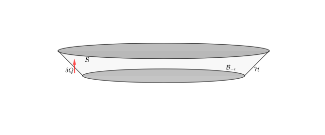
Figure 2: A sketch of a slice of a light-cone cut LCD. We denote the spatial cross-sections at times $t=-\epsilon$ and $t=0$ by $\mathcal{B}_{-\epsilon}$ and $\mathcal{B}$, respectively. The red arrow depicts the physical heat flux $\delta Q$ across the slice’s null boundary $\mathcal{H}$.

There are two contributions to the total change of the LCD’s entropy. First, the Clausius entropy of the matter inside the LCD changes due to the heat flux across the horizon. To compute the corresponding change in the Clausius entropy, we simply have to integrate equation (11) for the time derivative of the Clausius entropy from $t=-\epsilon$ to $t=0$. We obtain

$$\Delta S_{\text{C}}=\frac{2\pi}{\hbar}\hat{T}_{\mu\nu}\left(P\right)\int_{-\epsilon}^{0}\text{d}tt\left(l+t\right)^{D-2}\int_{\mathcal{B}_{t}}\text{d}\Omega_{D-2}\hat{k}_{-}^{\mu}\hat{k}_{-}^{\nu},$$ (43)

where we used that both the angular integration element $\text{d}\Omega_{D-2}$ and the null normal $\hat{k}_{-}^{\mu}$ are time-independent to split the integration in two parts. For the angular integral, we consider that $\hat{k}_{-}^{\mu}=\hat{n}^{\mu}+\hat{m}^{\mu}$, where $\hat{n}^{\mu}=\delta^{\mu}_{t}$ is the timelike normal to $\mathcal{B}_{t}$ and $\hat{m}^{\mu}$ the spacelike normal to it (i.e., the radial unit vector). It holds, up to subleading corrections due to spacetime curvature,

$$\int\hat{m}^{\mu}\text{d}\Omega_{D-2} =0,\,$$

$$\int\hat{m}^{\mu}\hat{m}^{\nu}\text{d}\Omega_{D-2} =\frac{\Omega_{D-2}}{D-1}\left(\hat{n}^{\mu}\hat{n}^{\nu}+\hat{g}^{\mu\nu}\right).$$ (44)

Here, and in the following, we evaluate all the tensors at point $P$. Performing the angular integration yields

$$\int\hat{k}_{-}^{\mu}\hat{k}_{-}^{\nu}\text{d}\Omega_{D-2}=\frac{\Omega_{D-2}}{D-1}\left(D\hat{n}^{\mu}\hat{n}^{\nu}+\hat{g}^{\mu\nu}\right).$$ (45)

Note that this expression is traceless. The time integral in equation (43) is straightforward. In total, we obtain

$$\Delta S_{\text{C}}=-\epsilon^{2}\frac{\pi\Omega_{D-2}l^{D-2}}{\hbar\left(D-1\right)}\hat{T}_{\mu\nu}\left(D\hat{n}^{\mu}\hat{n}^{\nu}+\hat{g}^{\mu\nu}\right)+O\left(\epsilon^{2}l^{D}\right).$$ (46)

We expanded the result in the small time interval $\epsilon$, discarding all the subleading $O\left(\epsilon^{3}\right)$ terms. The $O\left(\epsilon^{2}l^{D}\right)$ corrections account for the approximation of the energy-momentum tensor by its value in the LCD’s centre $P$ and for neglecting the curvature effects (captured by the Riemann normal coordinate expansion of the metric (1)). In principle, these corrections can be worked out explicitly, but since we assume that $l$ is much smaller than the local curvature length scale, their effect is negligible.

The second contribution to the change in LCD’s entropy comes from the expansion of its horizon. As we argued in subsection II.3, the LCD’s horizon possesses entropy proportional to its area, $S=\eta\hat{\mathcal{A}}$. Hence, the entropy associated with the horizon (regardless of its microscopic interpretation) changes with its expansion. To compute this change of entropy, it becomes advantageous to consider a light-cone cut LCD, which specifies the past null boundary of the LCD [47]. Then, we can easily compute the difference in the area of the boundary’s spatial (i.e., orthogonal to the vector field $\hat{n}^{\mu}$) cross-sections at different times, in our case at $t=-\epsilon$ and $t=0$. The simplest way to do it is by considering the expansion of the congruence of the null boundary generators $\hat{k}^{\mu}_{-}$, i.e., $\theta=\hat{\nabla}_{\mu}\hat{k}^{\mu}_{-}$. By definition of the expansion, it then holds for the change of area between times $t=-\epsilon$ and $t=0$ [90, 17, 47]

$$\Delta\hat{\mathcal{A}}=\int_{-\epsilon}^{0}\text{d}s\int\text{d}^{D-2}\hat{\mathcal{A}}\,\theta,$$ (47)

with $s$ being the null parameter along the horizon generators. The evolution of $\theta$ obeys the Raychaudhuri equation [90]

$$\dot{\theta}=-\frac{1}{D-2}\theta^{2}-\sigma^{2}-\hat{R}_{\mu\nu}\hat{k}_{-}^{\mu}\hat{k}_{-}^{\nu},$$ (48)

where we introduced the shorthand $\dot{\theta}=\text{d}\theta/\text{d}s$. The second term on the right hand side $\sigma^{2}=\sigma_{\mu\nu}\sigma^{\mu\nu}$ corresponds to the shear of the congruence

$$\sigma_{\mu\nu}=\hat{h}_{\mu}^{\;\>\lambda}\hat{h}_{\nu}^{\;\>\rho}\hat{\nabla}_{(\lambda|}\hat{k}_{-|\rho)}-\frac{1}{D-2}\hat{\nabla}_{\rho}\hat{k}_{-}^{\rho}\hat{h}_{\mu\nu},$$ (49)

with $\hat{h}_{\mu\nu}$ being the induced metric on the null boundary (the shear does not depend on its precise choice). The twist of the congruence vanishes because it generates a surface. The shear tensor evolves according to the following equation

$$\dot{\sigma}_{\mu\nu}=-\frac{2}{D-2}\theta\sigma_{\mu\nu}-\hat{C}_{\lambda\rho\sigma\tau}\hat{k}_{-}^{\lambda}\hat{k}_{-}^{\sigma}\hat{h}_{\mu}^{\rho}\hat{h}_{\nu}^{\tau},$$ (50)

where $\hat{C}_{\lambda\rho\sigma\tau}$ is Weyl curvature tensor. The horizon of an LCD in flat spacetime has an identically vanishing shear. However, its expansion equals $\theta_{\text{flat}}\left(s\right)=\left(D-2\right)/\left(l+s\right)$ [47]. The curvature-dependent terms in the evolution equations for $\theta$ and $\sigma_{\mu\nu}$ do not contain any further terms inversely proportional to $s$. Thence, we can expand $\theta$ and $\sigma_{\mu\nu}$ in powers of $s$ in the following way (note that $-\epsilon\leq s\leq 0$)

$$\theta =\theta_{\text{flat}}+\theta_{(0)}+s\theta_{(1)}+O\left(s^{2}\right),$$ (51)

$$\sigma_{\mu\nu} =\sigma_{(0)\mu\nu}+s\sigma_{(1)\mu\nu}+O\left(s^{2}\right).$$ (52)

In general, $\theta_{(0)}$ and $\sigma_{(0)\mu\nu}$ represent $D\left(D+1\right)/2$ arbitrary functions. However, it has been shown that one can refine the construction of a light-cone cut LCD [15, 16]. While the motivation in that case has been the use of the conformal Killing identity rather than the Raychaudhuri equation, it also involves fixing $D\left(D+1\right)/2$ arbitrary functions. Therefore, translating the results of that analysis to the language of the Rauchaudhuri equation implies that we are free to set up our LCD so that $\theta_{(0)}=\sigma_{(0)\mu\nu}=0$. In principle, we might also keep $\theta_{(0)}$ and $\sigma_{(0)\mu\nu}$ arbitrary. In that case, a previous analysis suggest that they would correspond to non-equilibrium entropy production [22]. The outcome of the derivation remains the same regardless of whether we keep $\theta_{(0)}$ and $\sigma_{(0),\mu\nu}$ arbitrary or not. Nevertheless, for the sake of clarity, we proceed assuming that we defined our light-cone cut LCD so that $\theta_{(0)}=\sigma_{(0)\mu\nu}=0$.

Plugging the ansatze (51) and (52) for the expansion and the shear into the evolution equations (48) and (50) yields the following solution

$$\theta =\theta_{\text{flat}}-s\hat{R}_{\mu\nu}\hat{k}_{-}^{\mu}\hat{k}_{-}^{\nu}+O\left(s^{2}\right),$$ (53)

$$\sigma_{\mu\nu} =-s\hat{C}_{\lambda\rho\sigma\tau}\hat{k}_{-}^{\lambda}\hat{k}_{-}^{\sigma}\hat{h}_{\mu}^{\rho}\hat{h}_{\nu}^{\tau}+O\left(s^{2}\right).$$ (54)

The flat spacetime expansion $\theta_{\text{flat}}$ is clearly not related to the spacetime curvature. Moreover, the area change proportional to $\theta_{\text{flat}}$ occurs even in vacuum, with no Clausius entropy flux across the horizon $\mathcal{H}$. Thence, we split the area change in two parts, one proportional to $\theta_{\text{flat}}$, the other to $\theta_{\text{curv}}=-s\hat{R}_{\mu\nu}\hat{k}_{-}^{\mu}\hat{k}_{-}^{\nu}$. Only the latter part can correspond to equilibrium change in the entropy of the horizon that is balanced by a matter entropy flux (see also [15, 16] for an alternative interpretation of $\theta_{\text{flat}}$ in terms of an irreversible thermodynamic process).

To compute the equilibrium change in area corresponding to $\theta_{\text{curv}}$ between times $t=-\epsilon$ and $t=0$ we now simply need to substitute $\theta_{\text{curv}}$ into equation (47), obtaining

$$\Delta\hat{\mathcal{A}}_{\text{curv}}= -\frac{\epsilon^{2}}{2}\int\hat{R}_{\mu\nu}\hat{k}_{-}^{\mu}\hat{k}_{-}^{\nu}\text{d}^{D-2}\hat{\mathcal{A}}+O\left(\epsilon^{2}l^{D}\right),$$

$$= -\epsilon^{2}\frac{\Omega_{D-2}l^{D-2}}{2\left(D-1\right)}\hat{R}_{\mu\nu}\left(D\hat{n}^{\mu}\hat{n}^{\nu}+\hat{g}^{\mu\nu}\right)+O\left(\epsilon^{2}l^{D}\right),$$ (55)

where we approximate the Ricci tensor by its value in $P$, leading to an $O\left(\epsilon^{2}l^{D}\right)$ error. Further errors of the same order appear due to neglecting the subleading terms in the Riemann normal coordinate expansion of the metric. The equilibrium change of the horizon entropy then equals $\Delta S_{\text{curv}}=\eta\Delta\hat{\mathcal{A}}_{\text{curv}}$.

The total equilibrium change in entropy vanishes, which implies $\Delta S_{\text{curv}}+\Delta S_{\text{C}}=0$. After some straightforward simplifications, this condition becomes

$$\left(\hat{R}_{\mu\nu}-\frac{1}{D}\hat{R}\hat{g}_{\mu\nu}-\frac{2\pi}{\eta\hbar}\hat{T}_{\mu\nu}+\frac{2\pi}{\eta\hbar}\frac{1}{D}\hat{T}\hat{g}_{\mu\nu}\right)\hat{n}^{\mu}\hat{n}^{\nu}=0,$$ (56)

valid at the point $P$. The construction of a light-cone cut causal LCD and derivation of equation (56) can be performed for every unit, timelike vector field $\hat{n}^{\mu}$ defined in $P$. Since equation (56) holds for an arbitrary unit, timelike vector, it implies (see the proof in appendix B)

$$\hat{R}_{\mu\nu}-\frac{1}{D}\hat{R}\hat{g}_{\mu\nu}\bigg{|}_{P}=\frac{2\pi}{\eta\hbar}\left(\hat{T}_{\mu\nu}-\frac{1}{D}\hat{T}\hat{g}_{\mu\nu}\right)\bigg{|}_{P}.$$ (57)

We assume that the strong equivalence principle holds. Consequently, $\eta$ is a universal constant. Furthermore, equations (57) can be derived at any regular spacetime point and have the same form at every point $P$. Finally, by considering the Newtonian limit of equations (57), we may define the Newton gravitational constant in terms of $\eta$, i.e., $G=1/\left(4\hbar\eta\right)$. The horizon entropy $S=\eta\hat{\mathcal{A}}$ then agrees with the Bekenstein entropy prescription $S_{\text{B}}=\hat{\mathcal{A}}/4\hbar G$.

In total, we have derived the following traceless equations governing gravitational dynamics

$$\hat{R}_{\mu\nu}-\frac{1}{D}\hat{R}\hat{g}_{\mu\nu}=8\pi G\left(\hat{T}_{\mu\nu}-\frac{1}{D}\hat{T}\hat{g}_{\mu\nu}\right).$$ (58)

Taking the divergence of equations (58) and invoking Bianchi identities implies $\hat{\nabla}_{\nu}\hat{T}_{\mu}^{\;\>\nu}=\hat{\nabla}_{\mu}\mathcal{J}$, where $\mathcal{J}$ is an arbitrary function. Then, we obtain the following divergenceless equations

$$\hat{R}_{\mu\nu}-\frac{1}{2}\hat{R}\hat{g}_{\mu\nu}+\Lambda\hat{g}_{\mu\nu}=8\pi G\hat{T^{\prime}}_{\mu\nu},$$ (59)

where $\Lambda$ is an arbitrary integration constant and $\hat{T^{\prime}}_{\mu\nu}=\hat{T}_{\mu\nu}-\mathcal{J}\hat{g}_{\mu\nu}$. We stress that the equations for gravitational dynamics we obtain from thermodynamics are the traceless ones (58), equations (59) only arise by integrating them. Therefore, the cosmological constant $\Lambda$ is only meaningful on shell and in principle varies between the solutions.

Up to this point, we have been agnostic about the local symmetries of our setup. Now, upon deriving the equations for gravitational dynamics, we are in a position to discuss the possible symmetry groups. Equations (59) contain the metric $\hat{g}_{\mu\nu}$ as the only gravitational degree of freedom. Since $\hat{g}_{\mu\nu}$ is a symmetric tensor, it can have at most $D\left(D+1\right)/2$ local symmetries. Assuming that we do not introduce any gauge fixing, we have only two choices compatible with the strong equivalence principle; the Diff and the WTDiff groups. We can understand the privileged position of these two groups in the following way: the strong equivalence principle can only be incorporated in theories that only have two propagating degrees of freedom, the ones associated with a massless graviton [23, 86]. Let us suppose that we write down a representation for a massless graviton with two physical polarisations in flat spacetime. We want to describe such a graviton by a symmetric, rank $2$ tensor that carries the maximum amount of gauge symmetry, i.e., we do not wish to introduce any gauge fixing. Then, the gauge group can be either Diff or WTDiff and the corresponding linearised action corresponds either to general relativity or to Weyl transverse gravity, respectively [24]. This perspective singles out general relativity and Weyl transverse gravity as the only gravitational theories with two propagating degrees of freedom (the massless graviton) and the maximum amount of gauge symmetry. It then follows that these two theories are the only ones compatible with the strong equivalence principle.

We cannot directly study the local symmetries using thermodynamics of spacetime, but we are nevertheless able to argue for its consitency with the WTDiff group. The key point is that the local causal horizons (regardless of their specific realisation) are insensitive to the overall conformal factor of the metric, which does not change the causal structure. Consequently, only the traceless equations (58) directly follow from the equilibrium condition (56). These indeed fix the dynamical metric $g_{\mu\nu}$ only up to the overall conformal factor. However, they suffice to recover the $D\left(D-1\right)/2$ components of the WTDiff-invariant auxiliary metric $\tilde{g}_{\mu\nu}$. Equations (58) are then fully consistent (together with the matter equations of motion, of course) without any further assumptions only if we write them in terms of the WTDiff-invariant auxiliary tensors. Therefore, they coincide with the equations of motion of Weyl transverse gravity (24).

Moreover, the gravitational equations we derived are encoded in the change of the horizon entropy. Then, shifting entropy by a universal constant has no effect on the gravitational dynamics. In a previous work, we have shown on the example of a de Sitter horizon that its entropy is indeed only defined up to a universal constant in Weyl transverse gravity [8]. However, we apparently have no freedom to similarly shift the horizon entropy in general relativity.

Finally, suppose we want to write an effective Lagrangian that implies the traceless equations (58) we derived from thermodynamics. If gravity is a fundamental interaction, such a Lagrangian should exist and play an important role in the quantum theory (as it does in loop quantum gravity or path integral quantum gravity). If gravity is emergent, we still find it reasonable to expect that we can write some effective classical Lagrangian for it. However, there exists no Diff-invariant metric (with or without extra fields) Lagrangian whose equations of motion are the traceless equations (58) [91] (although non-metric proposals for the variational principle have been put forward [12, 92]). At the same time, equations (58) coincide with the equations of motion obtained from the Weyl transverse gravity Lagrangian (19). Therefore, assuming that equations (58) we derived from thermodynamics are the Euler-Lagrange equations of some metric action, we are uniquely led to Weyl transverse gravity.

In principle, we have no a priori reason to expect that thermodynamics of spacetime (together with the equivalence principle) recovers all the information about gravitational dynamics. Perhaps some information, i.e., the local energy-momentum conservation and a fixed off-shell value of the cosmological constant indeed needs to be added, allowing us to obtain a Diff-invariant description of gravity. Nevertheless, the apparent strong connection between thermodynamics and gravity makes it worthwhile to ask what happens if they are in fact fully equivalent. And pursuing this question leads us directly to Weyl transverse gravity. Remarkably, this theory is also supported by a number of arguments completely independent of thermodynamics. First, the field theoretic approach to gravity [24, 30, 25] singles out Weyl transverse gravity and general relativity, putting both theories on the same ground. Furthermore, in section IV we have shown that Weyl transverse gravity and general relativity are apparently the only two theories of gravity in four spacetime dimensions satisfying the strong equivalence principle. Moreover, in contrast to general relativity, Weyl transverse gravity also offers a robust solution to the problem of the vacuum energy contributions to the cosmological constant [76, 32].

In conclusion, thermodynamics of spacetime encodes the traceless equations of motion of Weyl transverse gravity (24). All the hatted quantities we used throughout the derivation ought to be understood as being WTDiff-invariant, i.e., defined with respect to the auxiliary metric tensor $\tilde{g}_{\mu\nu}=\hat{g}_{\mu\nu}$.

V.2 Semiclassical dynamics: entanglement equilibrium approach

To strengthen our case for Weyl transverse gravity, we also analyse its consistence with the entanglement equilibrium approach to derive the equations governing the gravitational dynamics. This derivation is independent of the physical process one that we studied in the previous subsection. The precise relation between both approaches is subtle and not yet completely understood. We discuss it in subsection VI.3 after showing how both derivations work in the context of modified theories of gravity.

The entanglement equilibrium approach phrases the local equilibrium conditions fully in terms of perturbations of the total quantum von Neumann entropy [43]. There are two contributions to the total entropy perturbation, one coming from the matter fields and the other one from the entanglement entropy of the horizon, proportional to its area $S=\eta\hat{\mathcal{A}}$.

On the one hand, this method has the drawback of relying on a specific interpretation of the horizon entropy. On the other hand, it has the advantage of using the same (von Neumann) definition both for entropy of the horizon and of matter. The entanglement equilibrium approach also becomes particularly natural in the AdS/CFT paradigm [93, 94, 95], in which the entropy of a causal horizon can be manifestly accounted for in terms of von Neumann entropy (via the Ryu-Takayanagi formula [96]). However, we instead consider the completely general spacetime setting, following the seminal paper [43].

We start with a geodesic LCD in its equilibrium state. It has been proposed that the appropriate local equilibrium state corresponds to a vacuum, maximally symmetric spacetime with curvature $\hat{G}^{\text{MSS}}_{\mu\nu}=-\lambda\hat{g}^{\text{MSS}}_{\mu\nu}$ [43] (so that, if this spacetime was a solution of the equations of motion of either general relativity or Weyl transverse gravity, $\lambda$ would correspond to the cosmological constant). In principle, the local value of $\lambda$ depends both on the position of the LCD and on its size parameter $l$. The equilibrium condition involves both the background and the value of the possible perturbations. This means that only a certain background corresponds to the equilibrium state. More explicitly, the equilibrium condition $\delta S=0$ ($S$ being the total entropy of the LCD) not only constrains the allowed perturbations, but also provides the value of $\lambda$ corresponding to the equilibrium state. In other words, $\lambda$ is determined by the perturbation of the corresponding state being isoentropic, i.e., the net change of the LCD’s entropy due to perturbation vanishing to the first order. We determine the equilibrium $\lambda$ only at the end of our derivation, keeping its value unspecified for the time being.

Taking the LCD in this equilibrium state, we introduce a small arbitrary perturbation of the metric $\delta\hat{g}_{\mu\nu}$ and of the matter fields, leading to a non-zero perturbation of the expectation value of the energy-momentum tensor, $\delta\langle\hat{T}^{\mu\nu}\rangle$. Once again, we proceed without presuming anything about the local symmetries of our setup. Since choosing the WTDiff symmetry group would also generically imply variations of the cosmological constant, we further allow the possibility of a small variation of the local curvature, $\delta\lambda$ (that would vanish in the Diff-invariant case).

For a perturbed equilibrium state, the total entropy perturbation by definition vanishes to the leading order, i.e., $\delta S_{\text{vN}}+\eta\delta\hat{\mathcal{A}}=0$ (the strong equivalence principle implies $\delta\eta=0$). We now evaluate both terms in this equilibrium condition. For the von Neumann entropy of non-conformal matter fields perturbed away from their vacuum state, we employ equation (15)

$$\delta S_{\text{vN}}=\frac{2\pi}{\kappa}\int_{\Sigma_{0}}\delta\langle\hat{T}^{\mu\nu}\rangle\zeta_{\mu}\hat{n}_{\nu}\text{d}^{D-1}\hat{\Sigma}+O\left(l^{D+2}\right)+\delta\hat{X}.$$ (60)

We remind the reader that this expression only works for matter fields with a fixed ultraviolet point near which the field behaves approximately like a conformal one. Other situations are not covered by the derivation we discuss [43, 40, 41].

To evaluate the second term in the equilibrium condition, $\eta\delta\hat{\mathcal{A}}$, we need to compute the perturbation of the area of the horizon’s spatial cross-section $\mathcal{B}$ corresponding to $t=0$. The area of $\mathcal{B}$ can be computed by expanding the integration element $\text{d}^{D-2}\hat{\mathcal{A}}$ in the Riemann normal coordinates (1), yielding [43]

$$\hat{\mathcal{A}}_{\mathcal{B}} =\!\int_{\mathcal{B}}\!\left(1\!-\!\frac{1}{6}l^{2}\hat{R}^{\mu}_{\;\>\nu\rho\sigma}\hat{m}^{\nu}\hat{m}^{\sigma}\hat{h}^{\rho}_{\mu}\right)l^{D-2}\text{d}\Omega_{D-2}+O\left(l^{D+2}\right)$$

$$=\Omega_{D-2}l^{D-2}\left[1\!-\!\frac{l^{2}}{6\left(D-1\right)}\hat{R}^{\mu}_{\;\>\nu\rho\sigma}\hat{h}^{\nu\sigma}\hat{h}^{\rho}_{\mu}\right]+O\left(l^{D+2}\right),$$ (61)

where we used equation (44) to carry out the angular integration of the unit radial vectors $\hat{m}^{\mu}$. Furthermore, it is easy to show that $\hat{R}^{\mu}_{\;\>\nu\rho\sigma}\hat{h}^{\nu\sigma}\hat{h}^{\rho}_{\mu}=2\hat{G}_{\mu\nu}\hat{n}^{\mu}\hat{n}^{\nu}$ [43], and we obtain

$$\hat{\mathcal{A}}_{\mathcal{B}}=\Omega_{D-2}l^{D-2}\left[1-\frac{l^{2}}{3\left(D-1\right)}\hat{G}_{\mu\nu}\hat{n}^{\mu}\hat{n}^{\nu}\right]+O\left(l^{D+2}\right).$$ (62)

In the unperturbed, maximally symmetric spacetime, it holds $\hat{G}^{\text{MSS}}_{\mu\nu}=-\lambda\hat{g}^{\text{MSS}}_{\mu\nu}$ and we get

$$\hat{\mathcal{A}}_{\mathcal{B},\text{MSS}}=\Omega_{D-2}l^{D-2}\left[1+\frac{l^{2}}{3\left(D-1\right)}\lambda\right]+O\left(l^{D+2}\right).$$ (63)

Performing the Riemann normal coordinate expansion of the perturbed metric we obtain the expression for the area of $\mathcal{B}$ in the perturbed metric

$$\hat{\mathcal{A}}_{\mathcal{B}}= ~{}\Omega_{D-2}l^{D-2}\bigg{[}1-\frac{l^{2}}{3\left(D-1\right)}\hat{G}_{\mu\nu}\hat{n}^{\mu}\hat{n}^{\nu}+\frac{D-2}{l}\delta l$$

$$-\frac{Dl}{3\left(D-1\right)}\hat{G}_{\mu\nu}\hat{n}^{\mu}\hat{n}^{\nu}\delta l\bigg{]}+O\left(l^{D+2}\right),$$ (64)

where $\hat{G}_{\mu\nu}$ stands for the Einstein tensor of the perturbed metric and we allowed for perturbations of the size parameter $l$. The perturbation of the area is then given by the difference of both expressions, i.e.,

$$\delta\hat{\mathcal{A}}_{\mathcal{B}}= ~{}\Omega_{D-2}l^{D-2}\bigg{[}-\frac{l^{2}}{3\left(D-1\right)}\left(\hat{G}_{\mu\nu}\hat{n}^{\mu}\hat{n}^{\nu}-\lambda\right)$$

$$+\frac{D-2}{l}\delta l-\frac{Dl}{3\left(D-1\right)}\hat{G}_{\mu\nu}\hat{n}^{\mu}\hat{n}^{\nu}\delta l\bigg{]}+O\left(l^{D+2}\right).$$ (65)

We have mentioned that defining a Euclidean canonical ensemble for an LCD relies on a fixed spatial volume condition [61, 62]. Likewise, the first law of LCDs includes a contribution from the volume perturbation, that has the form of a work term in the standard first law of thermodynamics [43, 3, 8]. From both perspectives we can expect that the equilibrium relation, $\delta S_{\text{vN}}+\eta\delta\hat{\mathcal{A}}=0$, holds only when the spatial volume is held fixed. The volume perturbation can be computed in the same way as the area perturbation and reads [43]

$$\delta\hat{\mathcal{V}}_{\Sigma_{0}}= ~{}\Omega_{D-2}l^{D-1}\bigg{[}-\frac{l^{2}}{3\left(D^{2}-1\right)}\left(\hat{G}_{\mu\nu}\hat{n}^{\mu}\hat{n}^{\nu}-\lambda\right)+\frac{\delta l}{l}$$

$$-\frac{l}{3\left(D-1\right)}\hat{G}_{\mu\nu}\hat{n}^{\mu}\hat{n}^{\nu}\delta l\bigg{]}+O\left(l^{D+3}\right).$$ (66)

Therefore, $\delta\hat{\mathcal{V}}_{\Sigma_{0}}=0$ implies

$$\delta l=\frac{l^{3}}{3\left(D^{2}-1\right)}\left(\hat{G}_{\mu\nu}\hat{n}^{\mu}\hat{n}^{\nu}-\lambda\right)+O\left(l^{D+3}\right),$$ (67)

and the area perturbation at constant volume becomes

$$\delta\hat{\mathcal{A}}_{\mathcal{B}}|_{\hat{\mathcal{V}}}=-\frac{\Omega_{D-2}l^{D}}{D^{2}-1}\left(\hat{G}_{\mu\nu}\hat{n}^{\mu}\hat{n}^{\nu}-\lambda\right)+O\left(l^{D+2}\right).$$ (68)

We now have everything we need to evaluate the equilibrium condition $\delta S_{\text{vN}}+\eta\delta\hat{\mathcal{A}}|_{\hat{\mathcal{V}}}=0$. It reads, up to $O\left(l^{D+2}\right)$ subleading terms,

$$\frac{2\pi}{\hbar}\left(\delta\langle\hat{T}_{\mu\nu}\rangle\hat{n}^{\mu}\hat{n}^{\nu}+\delta\hat{X}\right)-\eta\left(\hat{G}_{\mu\nu}\hat{n}^{\mu}\hat{n}^{\nu}-\lambda\right)=0,$$ (69)

from which we obtain

$$8\pi G\left(\delta\langle\hat{T}_{\mu\nu}\rangle-\delta\hat{X}\hat{g}_{\mu\nu}\right)-\hat{G}_{\mu\nu}-\lambda\hat{g}_{\mu\nu}=0,$$ (70)

where we again defined the Newton constant in terms of $\eta$, as $G=1/\left(4\hbar\eta\right)$, and the arbitrariness of the unit, timelike vector field $\hat{n}^{\mu}$ allowed us to remove the contractions with $\hat{n}^{\mu}$ (for the proof, see appendix B).

To complete the derivation, we need to determine the equilibrium value of the local curvature $\lambda$ which corresponds to an isoentropic perturbation. To do so, we simply take the trace of equations (70), obtaining

$$\lambda=8\pi G\left(\frac{1}{D}\delta\langle\hat{T}\rangle-\delta\hat{X}\right)+\frac{D-2}{2D}\hat{R},$$ (71)

i.e. the equilibrium value of $\lambda$ corresponds to a combination of the scalar curvature and terms determined by the perturbation of the matter fields. As an aside, for conformal matter fields satisfying the local energy conservation, we have $\delta\langle\hat{T}\rangle=\delta\hat{X}=0$, which leads to a much simpler expression for $\lambda$, namely $\lambda=\left(D-2\right)\hat{R}/\left(2D\right)$. Then, the scalar curvature of the unperturbed, locally maximally symmetric spacetime and the perturbed spacetime are equal and we have $\delta\hat{R}=0$.

Finally, plugging $\lambda$ into equations (70) yields the traceless equations governing the gravitational dynamics

$$\hat{R}_{\mu\nu}-\frac{1}{D}\hat{R}=8\pi G\left(\delta\langle\hat{T}_{\mu\nu}\rangle-\frac{1}{D}\delta\langle\hat{T}\rangle\hat{g}_{\mu\nu}\right),$$ (72)

valid at the point $P$. The strong equivalence principle guarantees that these equations hold throughout the spacetime.

A subtle issue should be noted. The curvature of the perturbed spacetime includes the contribution of $\lambda$. Equation (71) connects $\lambda$ with $\delta\hat{X}$, which in general explicitly depends on the arbitrary size parameter $l$ of the LCD [43, 41, 40]. Then, the traceless Ricci tensor also depends on $l$ and this arbitrary parameter enters the equations governing the gravitational dynamics. This issue does not occur for conformally invariant matter fields which obey $\delta\hat{X}=0$.

All the arguments we gave in the previous subsection for the recovery of Weyl transverse gravity apply here as well. In particular, we again rely on the construction of a local causal diamond which is insensitive to the overall conformal factor of the metric, leading to the Weyl invariance of the resulting equations. Moreover, since the equations are traceless, they do not explicitly enforce the local energy conservation and the cosmological constant appears as an on shell integration constant, just like in Weyl transverse gravity. Lastly, the derivation is again insensitive to the shifts of entropy by a universal constant, just like in Weyl transverse gravity [8].

Notably, the equations governing the gravitational dynamics we derived have the quantum expectation value of the energy-momentum tensor as a source for the classical spacetime curvature. Therefore, we have in fact obtained the semiclassical traceless equations for Weyl transverse gravity.

VI Equations of motion from Wald entropy in WTDiff-invariant gravity

In the previous section, we have argued that thermodynamics of LCDs encodes (semi)classical gravitational dynamics equivalent to Weyl transverse gravity. For Diff-invariant gravity it has been further shown that thermodynamics also encodes the equations of motion of any gravitational theory whose Lagrangian is a function of only the metric and the Riemann tensor [14, 15, 16]. The derivation of this result uses the Wald entropy prescription [4, 5] corresponding to the given Lagrangian as an input. Then, one expects that the equations of motion for any WTDiff-invariant Lagrangian constructed from the auxiliary metric and Riemann tensor should also be obtainable in this way. Otherwise, the correspondence between thermodynamics and WTDiff symmetry we established in the previous section would be called into question, as it would be unable to reproduce all the results available in the Diff-invariant setup.

It is not immediately clear that the recovery of the equations of motion for modified WTDiff-invariant theories from their Wald entropy is possible. The first technical issue we face is that the original definition of Wald entropy in the covariant phase space approach applies only to local, Diff-invariant theories of gravity [4, 5]. Thus, the first necessary step we already performed was to extend the covariant phase space construction and the definition of Wald entropy to arbitrary local, WTDiff-invariant theories of gravity in [8, 9]. Extending the covariant phase space formalism was necessary, but not sufficient by itself, since applying the resulting Wald entropy prescription to an LCD is not straightforward as we explain in the following. The conformal Killing vector $\zeta^{\mu}$ (3) of an LCD clearly generates an infinitesimal diffeomorphism, which makes it a local symmetry generator for Diff-invariant gravity. However, $\zeta^{\mu}$ does not in general generate a transformation belonging to the WTDiff group (see, e.g. [31, 8] for longer discussions of this subtlety). One then has to be careful in applying the results of the covariant phase space construction to $\zeta^{\mu}$, since it does not correspond to a local symmetry of WTDiff-invariant gravity [97, 8, 9]. Nevertheless, $\zeta^{\mu}$ lies in the WTDiff group in a flat background (it generates a Weyl transformation of the dynamical metric $g_{\mu\nu}$). Using this observation, we showed that the WTDiff-invariant Wald entropy prescription indeed works for LCDs [8, 9]. Therefore, we can employ it to derive the equations governing the gravitational dynamics. As in the previous section, we perform the derivation by (the same) two different approaches: the physical process one and the entanglement equilibrium one.

Before proceeding, let us stress some general issues associated with applying the thermodynamic derivation to modified theories of gravity:

• To derive the equations for the gravitational dynamics from Wald entropy, we have to first specify the gravitational Lagrangian. Then, the derivation presents a somewhat circular argument as the Lagrangian already yields the equations of motion. Deriving the equations for gravitational dynamics from Wald entropy then shows that the boundary contribution to the variation of the action (which encodes Wald entropy) contains all the information necessary to reconstruct the gravitational dynamics. While this fact is of interest by itself, it does not allow us to learn anything genuinely new about the gravitational dynamics. One does not encounter this problem with entropy proportional to the horizon area, $S=\eta\tilde{\mathcal{A}}$, as we can provide robust, largely model-independent arguments for this form of the leading order entropy contribution (as we discuss in subsection II.3).

• The previous argument can be improved to not directly involve Wald entropy. Instead, one may assume that entropy of the horizon can be completely interpreted in terms of quantum entanglement (with all the drawbacks we discussed in subsection II.3). It has been shown that renormalising this entropy leads to subleading corrections to it [98, 99]. This renormalisation procedure yields both the renormalised entropy expression and an effective gravitational Lagrangian. It turns out that the renormalised entropy precisely agrees with Wald entropy corresponding to the effective Lagrangian. This argument provides a justification for using Wald entropy prescription without the need to specify the gravitational Lagrangian beforehand. Herein, we tacitly assume this interpretation of the procedure, although we work directly with Wald entropy prescription.

• The cosmological constant term in a Diff-invariant gravitational Lagrangian does not affect Wald entropy. Consequently, the equations one derives from thermodynamics fail to reproduce this term in the Lagrangian. Instead, the cosmological constant arises as an on-shell integration constant in the process of solving the equations and has no connection with the fixed parameter in the Lagrangian that would enter the Euler-Lagrange equations. This failure to completely reconstruct the information contained in the Lagrangian of course disappears in WTDiff-invariant gravity. In this case, both the Euler-Lagrange equations and the thermodynamically derived equations are traceless and unaffected by any constant parameter in the Lagrangian. Therefore, as we will show, both procedures to derive the gravitational equations are fully consistent with each other.

VI.1 Physical process approach

We first consider a physical process derivation. Our setup is essentially the same as in subsection V.1, i.e., we again study the change of entropy of a light-cone cut LCD between times $t=-\epsilon$ and $t=0$ (with $\epsilon\ll l$). Therefore, we consider a slice of the null boundary of the LCD sketched in figure 2. However, the Raychaudhuri equation approach we introduced in subsection V.1 does not straightforwardly generalise to generic Wald entropy expressions [38, 13]. Instead, we use the approach based on a conformal Killing identity [15, 16], which we adapt for the WTDiff-invariant setup.

The equations of motion are encoded in the equilibrium condition applied to the changes of the matter entropy and the Wald entropy of the horizon. We have already computed the change in matter Clausius entropy in subsection V.1, obtaining equation (46).

Wald entropy for the class of theories described by the action (32) obeys (see  [9] for a discussion of the subtleties involved in the defining it)

$$S_{\text{W}}\left(t\right) =\frac{2\pi}{\hbar\kappa}\int_{\mathcal{B}_{t}}Q^{\nu\mu}_{\zeta}\text{d}\tilde{B}_{\mu\nu},$$ (73)

$$Q^{\nu\mu}_{\zeta} =2\tilde{E}^{\nu\mu\rho}_{\quad\;\>\sigma}\tilde{\nabla}_{\rho}\zeta^{\sigma}-4\tilde{\nabla}_{\rho}\tilde{E}^{\nu\mu\rho}_{\quad\;\>\sigma}\zeta^{\sigma},$$ (74)

where $Q^{\nu\mu}_{\zeta}$ denotes the (background-dependent) Noether charge corresponding to the conformal Killing vector $\zeta^{\mu}$, we define the oriented area element $\text{d}\tilde{B}_{\mu\nu}=\left(\tilde{n}_{\mu}\tilde{m}_{\nu}-\tilde{n}_{\nu}\tilde{m}_{\mu}\right)\text{d}^{D-2}\tilde{\mathcal{A}}$ and $\tilde{E}_{\mu}^{\;\>\nu\rho\sigma}=\partial L/\partial\tilde{R}^{\mu}_{\;\>\nu\rho\sigma}$ has been introduced in equation (35). It is easy to see that the entropy of an LCD is time-dependent (its area expands). Then, even though $\zeta^{\mu}$ vanishes at the bifurcation surface $t=0$ of the LCD’s boundary (see equation (3)), the term proportional to $\zeta^{\mu}$ does contribute to entropy. Then, by applying the generalised Stokes theorem, we obtain for the change of Wald entropy between the spatial spheres $\mathcal{B}_{-\epsilon}$ and $\mathcal{B}$

$$\Delta S_{\text{W}}=\frac{2\pi}{\kappa}\int_{-\epsilon}^{0}\text{d}t\int_{\mathcal{B}_{t}}\text{d}^{D-2}\tilde{\mathcal{A}}\tilde{k}_{-}^{\mu}\tilde{\nabla}_{\nu}Q^{\nu\mu}_{\zeta},$$ (75)

where $\tilde{k}_{-}^{\mu}$ is a future-pointing, WTDiff-invariant null normal to the horizon.

Our strategy is to rewrite $\Delta S_{\text{W}}$ in a form that does not include derivatives of $\zeta^{\mu}$ (present in $\tilde{\nabla}_{\nu}Q^{\nu\mu}_{\zeta}$), which will allow us to straightforwardly carry out the integration. To remove the derivatives of $\zeta^{\mu}$, we invoke the (approximate) conformal Killing identity [16]

$$\tilde{\nabla}_{\nu}\tilde{\nabla}_{\rho}\zeta_{\sigma}= ~{}\tilde{R}_{\lambda\nu\rho\sigma}\zeta^{\lambda}+\frac{1}{D}\tilde{g}_{\rho\sigma}\tilde{\nabla}_{\nu}\tilde{\nabla}_{\lambda}\zeta^{\lambda}+\frac{1}{D}\tilde{g}_{\nu\sigma}\tilde{\nabla}_{\rho}\tilde{\nabla}_{\lambda}\zeta^{\lambda}$$

$$-\frac{1}{D}\tilde{g}_{\nu\rho}\tilde{\nabla}_{\sigma}\tilde{\nabla}_{\lambda}\zeta^{\lambda}+O(\epsilon^{2}l^{D}).$$ (76)

Applying this identity to equation (75) yields

$$\Delta S_{\text{W}}= ~{}\frac{4\pi}{\hbar\kappa}\int_{-\epsilon}^{0}\text{d}t\int_{\mathcal{B}_{t}}\text{d}^{D-2}\tilde{\mathcal{A}}\tilde{k}_{-}^{\mu}$$

$$\times\bigg{[}-\tilde{E}_{\nu}^{\;\>\lambda\rho\sigma}\tilde{R}_{\mu\lambda\rho\sigma}\zeta^{\nu}+2\tilde{\nabla}_{\rho}\tilde{\nabla}_{\sigma}\tilde{E}_{\mu\;\;\;\nu}^{\;\>\rho\sigma}\zeta^{\nu}$$

$$+\frac{64\pi G}{D}\tilde{\nabla}_{\rho}\tilde{\nabla}_{\lambda}\zeta^{\lambda}\tilde{E}_{\mu\nu}^{\;\>\;\>\rho\nu}\bigg{]}$$ (77)

where we discarded the $O\left(\epsilon^{3}\right)$ terms. In general, other contributions would appear due to the fact that $\zeta^{\mu}$ is only an approximate conformal Killing vector and does not precisely satisfy the conformal Killing identity (76). However, these extra terms can be removed by adding suitable curvature-dependent terms (which disappear in flat spacetime) to the definition of $\zeta^{\mu}$ (3). The procedure has been worked out in detail in the Diff-invariant setup and translates without any changes to the WTDiff-invariant case we consider [16].

The last term on the right hand side of equation (77) is the only one that does not vanish in flat spacetime. Therefore, much like in the special case of Weyl transverse gravity (see equation (55) and the accompanying discussion) we split the change of the Wald entropy in a flat spacetime contribution and a contribution induced by the spacetime curvature

$$\Delta S_{\text{W}}= \Delta S_{\text{flat}}+\Delta S_{\text{curv}},$$ (78)

$$\Delta S_{\text{flat}}= \frac{4\pi}{\hbar\kappa}\frac{4}{D}\int_{-\epsilon}^{0}\text{d}t\int_{\mathcal{B}_{t}}\text{d}^{D-2}\tilde{\mathcal{A}}\tilde{k}_{-}^{\mu}\tilde{\nabla}_{\rho}\tilde{\nabla}_{\lambda}\zeta^{\lambda}\tilde{E}_{\mu\nu}^{\;\;\;\>\rho\nu},$$ (79)

$$\Delta S_{\text{curv}}= \frac{1}{4\hbar G\kappa}\int_{-\epsilon}^{0}\text{d}t\int_{\mathcal{B}_{t}}\text{d}^{D-2}\tilde{\mathcal{A}}\tilde{k}_{-}^{\mu}\big{[}\tilde{E}_{\nu}^{\;\;\lambda\rho\sigma}\tilde{R}_{\mu\lambda\rho\sigma}$$

$$-2\tilde{\nabla}_{\rho}\tilde{\nabla}_{\sigma}\tilde{E}_{\mu\;\;\;\nu}^{\;\;\rho\sigma}\big{]}\zeta^{\nu}.$$ (80)

In the following, as in subsection V, we disregard the flat spacetime term $\Delta S_{\text{flat}}$. In any case, only $\Delta S_{\text{curv}}$ is connected with a matter Clausius entropy flux across the horizon. We thus study the thermodynamic equilibrium condition

$$\Delta S_{\text{C}}+\Delta S_{\text{curv}}=0.$$ (81)

The integrals in (80) can be performed straightforwardly to yield

$$\Delta S_{\text{curv}}= -\epsilon^{2}\frac{D\Omega_{D-2}}{8\hbar G\left(D-1\right)}l^{D-2}\left(\tilde{H}_{\mu\nu}-\frac{1}{D}\tilde{H}\tilde{g}_{\mu\nu}\right)\tilde{n}^{\mu}\tilde{n}^{\nu}$$

$$+O\left(\epsilon^{2}l^{D}\right),$$ (82)

where the $O\left(\epsilon^{2}l^{D}\right)$ terms come from the higher order contributions in the Riemann normal coordinate expansion and we identified the symmetric tensor $\tilde{H}_{\mu\nu}$ defined by equation (34).

Next, we plug this result and the expression (46) for $\Delta S_{\text{C}}$ into the equilibrium condition (81). Since, as before, $\tilde{n}^{\mu}$ is an arbitrary, timelike, unit, WTDiff-invariant vector field, we remove the contractions with it (see appendix B). Lastly, the Einstein equivalence principle guarantees that the resulting equations for gravitational dynamics valid in $P$ hold in every regular spacetime point, eliminating the dependence of the quantities on $P$. In total, we arrive at the following traceless equations valid throughout the spacetime

$$\tilde{H}_{\mu\nu}-\frac{1}{D}\tilde{H}\tilde{g}_{\mu\nu}=8\pi G\left(\tilde{T}_{\mu\nu}-\frac{1}{D}\tilde{T}\tilde{g}_{\mu\nu}\right).$$ (83)

We can see that we have reproduced the traceless equations of motion (33) of a local, WTDiff-invariant theory of gravity whose Lagrangian is an arbitrary function of $\tilde{g}_{\mu\nu}$ and $\tilde{R}^{\mu}_{\;\>\nu\rho\sigma}$. We stress that both the thermodynamically derived equations (83) and the Euler-Lagrange equations (33) are traceless and recover the cosmological constant as an on-shell integration constant. Thence, unlike in the Diff-invariant case, Wald entropy suffices to recover all the information contained in the WTDiff-invariant gravitational Lagrangian (32).

VI.2 Entanglement equilibrium approach

The entanglement equilibrium derivation we analysed in subsection V.2 can also be generalised to local, WTDiff-invariant theories of gravity given by the Lagrangian (32). Our treatment largely follows the method developed for Diff-invariant gravity [14], which we modify for the WTDiff-invariant setup.

The renormalised entanglement entropy associated with the horizon of a geodesic LCD takes the same form as the Wald entropy of certain modified gravity theories [98]. Therefore, we have the following entanglement equilibrium condition

$$\delta S_{\text{W}}+\delta S_{\text{vN}}=0,$$ (84)

where $\delta S_{\text{W}}$ denotes the Wald entropy perturbation, and the matter von Neumann entropy perturbation $\delta S_{\text{vN}}$ obeys equation (15). As we discussed in subsection V.2, the equilibrium state of the LCD corresponds to a locally maximally symmetric spacetime with curvature $\hat{G}^{\text{MSS}}_{\mu\nu}=-\lambda\hat{g}^{\text{MSS}}_{\mu\nu}$, where $\lambda$ in principle depends on the position and size of the LCD as before.

We now need to evaluate the perturbation of Wald entropy for the bifurcate $\left(n-2\right)$-surface $\mathcal{B}$ of the horizon. Then, plugging the result into the equilibrium condition (84) will allow us to obtain the equations of motion.

A generic perturbation of Wald entropy of $\mathcal{B}$ equals

$$\delta S_{\text{W}}=\frac{4\pi}{\hbar\kappa}\delta\int_{\mathcal{B}}\tilde{E}^{\nu\mu\rho}_{\quad\;\>\sigma}\tilde{\nabla}_{\rho}\zeta^{\sigma}\text{d}\mathcal{B}_{\mu\nu}.$$ (85)

Since $l$ is much smaller than the local curvature length scale, we can expand $\tilde{E}^{\nu\mu\rho}_{\quad\;\>\sigma}$ in powers of $l$ around the LCD’s centre $P$, keeping only the first three terms in the expansion

$$\delta S_{\text{W}}= ~{}\frac{4\pi}{\hbar\kappa}\delta\int_{\mathcal{B}}\bigg{(}\tilde{E}^{\nu\mu\rho}_{\quad\;\>\sigma}+l\tilde{m}^{\lambda}\tilde{\nabla}_{\lambda}\tilde{E}^{\nu\mu\rho}_{\quad\;\>\sigma}$$

$$+\frac{1}{2}l^{2}\tilde{m}^{\lambda}\tilde{m}^{\tau}\tilde{\nabla}_{\lambda}\tilde{\nabla}_{\tau}\tilde{E}^{\nu\mu\rho}_{\quad\;\>\sigma}\bigg{)}\tilde{\nabla}_{\rho}\zeta^{\sigma}\text{d}\mathcal{B}_{\mu\nu},$$ (86)

where $\tilde{m}^{\mu}$ is the WTDiff-invariant unit, spatial normal to $\mathcal{B}$, and we evaluate all the tensors at $P$. For computational convenience, we split $\tilde{E}^{\;\>\nu\rho\sigma}_{\mu}$ into the part corresponding to Weyl transverse gravity and the higher order corrections we denote by $\tilde{F}^{\;\>\nu\rho\sigma}_{\mu}$, i.e.,

$$\tilde{E}^{\;\>\nu\rho\sigma}_{\mu}=\frac{1}{32\pi G}\left(\delta^{\rho}_{\mu}\tilde{g}^{\nu\sigma}-\delta^{\sigma}_{\mu}\tilde{g}^{\nu\rho}+2\tilde{F}^{\;\>\nu\rho\sigma}_{\mu}\right).$$ (87)

Note that, since $\tilde{F}^{\;\>\nu\rho\sigma}_{\mu}$ vanishes in a maximally symmetric spacetime $\delta\tilde{F}^{\;\>\nu\rho\sigma}_{\mu}=\tilde{F}^{\;\>\nu\rho\sigma}_{\mu}$, so we obtain

$$\delta S_{\text{W}}= ~{}\frac{\delta\tilde{\mathcal{A}}_{\mathcal{B}}}{4\hbar G}-\frac{\Omega_{D-2}l^{D-2}}{4\hbar G\left(D-1\right)}\tilde{n}^{\mu}\tilde{n}^{\nu}$$

$$\times\bigg{[}\tilde{W}_{\mu\nu}-\frac{l^{2}}{\left(D+1\right)}\tilde{\nabla}_{\rho}\tilde{\nabla}_{\sigma}\tilde{F}^{\;\>\rho\sigma}_{\mu\;\;\;\>\nu}\bigg{]},$$ (88)

where $\tilde{F}^{\;\>\nu\rho\sigma}_{\mu}$ now corresponds to its value for the perturbed metric. To simplify the notation, we introduced a tensor

$$\tilde{W}_{\mu\nu}= ~{}\left(1+\frac{l^{2}}{2\left(D+1\right)}\tilde{h}^{\rho\sigma}\tilde{\nabla}_{\rho}\tilde{\nabla}_{\sigma}\right)\tilde{F}^{\lambda}_{\;\>\mu\lambda\nu},$$ (89)

whose significance will become clear in the following. Finally, the area variation equals the expression given by equation (65).

In the special case of Weyl transverse gravity, we have seen that the equilibrium condition (84) only applies to perturbations that hold fixed the WTDiff-invariant volume of the geodesic $\left(D-1\right)$-dimensional ball $\Sigma_{0}$ (as its perturbation corresponds to a work term in the first law of causal diamonds [3, 8, 9]). It has been shown that the former condition translates directly to the case of more general WTDiff-invariant theories of gravity [14]. However, rather than the spatial volume of $\Sigma_{0}$, one needs to keep fixed its generalised volume $\tilde{\mathcal{W}}$ [14, 9]

$$\tilde{\mathcal{W}}=\tilde{\mathcal{V}}+\frac{32\pi}{D-2}\int_{\Sigma_{0}}\tilde{F}^{\lambda}_{\;\>\mu\lambda\nu}\tilde{n}^{\mu}\tilde{n}^{\nu}\text{d}^{D-1}\Sigma,$$ (90)

where $\tilde{\mathcal{V}}$ denotes the geometric, WTDiff-invariant volume. For Weyl transverse gravity, $\tilde{F}^{\lambda}_{\;\>\mu\lambda\nu}$ vanishes and the generalised volume reduces to the geometric one. The generalised volume appears in the first law of LCDs in modified theories of gravity instead of the standard volume [14]. It also must be held fixed to define an LCD Euclidean canonical ensemble in modified theories of gravity [100]. Thence, it plays the same role for modified theories of gravity as the geometric WTDiff-invariant volume does for Weyl transverse gravity. In conclusion, the entanglement equilibrium condition (84) applies to perturbations obeying $\delta\tilde{\mathcal{W}}=0$.

Let us impose the condition of constant generalised volume, $\delta\tilde{\mathcal{W}}=0$, on the Wald entropy perturbation. Expanding the perturbation of the generalised volume (90) around $P$ in the same way as we have done for Wald entropy (equation (88)), we find

$$\delta\tilde{\mathcal{W}}_{\Sigma_{0}}=\delta\tilde{\mathcal{V}}_{\Sigma_{0}}+\frac{\Omega_{D-2}l^{D-1}}{4\left(D-1\right)\left(D-2\right)}\tilde{W}_{\mu\nu}\tilde{n}^{\mu}\tilde{n}^{\nu},$$ (91)

where $\delta\tilde{\mathcal{V}}_{\Sigma_{0}}$ denotes the perturbation of the WTDiff-invariant geometric volume and its expression was already given in equation (66). We can see that the previously introduced tensor $\tilde{W}_{\mu\nu}$ (89) quantifies the departure of the generalised volume perturbation from the geometric one.

The only way to satisfy the constraint $\delta\tilde{\mathcal{W}}_{\Sigma_{0}}=0$ is by choosing the variation $\delta l$ of the LCD’s size parameter to be

$$\delta l=\frac{l^{3}}{3\left(D^{2}-1\right)}\left(\tilde{G}_{\mu\nu}\tilde{n}^{\mu}\tilde{n}^{\nu}-\lambda\right)-\frac{l\tilde{W}_{\mu\nu}\tilde{n}^{\mu}\tilde{n}^{\nu}}{4\left(D-1\right)\left(D-2\right)}.$$ (92)

Plugging this expression for $\delta l$ into the general equation (88), the terms with $\tilde{W}_{\mu\nu}$ cancel out and we obtain for the perturbation of Wald entropy at fixed generalised volume

$$\delta S_{\text{W}}\big{|}_{\delta\tilde{\mathcal{W}}=0}= \frac{\Omega_{D-2}l^{D}}{4\hbar G\left(D^{2}-1\right)}\tilde{n}^{\mu}\tilde{n}^{\nu}$$

$$\times\Big{[}\tilde{G}_{\mu\nu}-\lambda\tilde{g}_{\mu\nu}+2\tilde{\nabla}_{\rho}\tilde{\nabla}_{\sigma}\tilde{F}^{\;\>\rho\sigma}_{\mu\;\;\;\>\nu}\Big{]}.$$ (93)

At this point, we have all the ingredients to evaluate the entanglement equilibrium condition (84). After some straightforward simplifications, it reads

$$\Big{[}\tilde{G}_{\mu\nu}-\lambda\tilde{g}_{\mu\nu}+2\tilde{\nabla}_{\rho}\tilde{\nabla}_{\sigma}\tilde{F}^{\;\>\rho\sigma}_{\mu\;\;\;\>\nu}$$

$$-8\pi G\left(\delta\langle\tilde{T}_{\mu\nu}\rangle-\delta\tilde{X}\right)\Big{]}\tilde{n}^{\mu}\tilde{n}^{\nu} =0.$$ (94)

We can once again remove the contractions with an arbitrary, unit timelike vector field $\tilde{n}^{\mu}$ (see Appendix B). Taking the trace of the equations determines the equilibrium value of $\lambda$ corresponding to an isoentropic perturbation

$$\lambda=8\pi G\left(\frac{1}{D}\delta\langle\tilde{T}\rangle-\delta\tilde{X}\right)+\frac{D-2}{2D}\tilde{R}+\frac{2}{D}\tilde{\nabla}_{\rho}\tilde{\nabla}_{\sigma}\tilde{F}^{\;\>\rho\lambda\sigma}_{\lambda}.$$ (95)

Plugging $\lambda$ back into the entanglement equilibrium condition (94), we obtain the traceless equations

$$\tilde{H}_{\mu\nu}^{(1)}-\frac{1}{D}\tilde{H}^{(1)}\tilde{g}_{\mu\nu}=8\pi G\left(\delta\langle\tilde{T}_{\mu\nu}\rangle-\frac{1}{D}\delta\langle\tilde{T}\rangle\tilde{g}_{\mu\nu}\right).$$ (96)

where we defined $\tilde{H}_{\mu\nu}^{(1)}$ as the part of the symmetric tensor $\tilde{H}_{\mu\nu}$ linear in the Riemann tensor, i.e.,

$$\tilde{H}_{\mu\nu}^{(1)}=\tilde{R}_{\mu\nu}+2\tilde{\nabla}_{\rho}\tilde{\nabla}_{\sigma}\tilde{F}^{\;\;\>\rho\sigma}_{(\mu\;\;\;\>\nu)}.$$ (97)

We used the fact that tensor $\tilde{F}^{\;\>\rho\sigma}_{\mu\;\;\;\>\nu}$ is itself at least linear in the Riemann tensor (as can be seen from equation (35) and the definition of $\tilde{F}^{\;\>\rho\sigma}_{\mu\;\;\;\>\nu}$ (87)). Therefore, we discarded any contractions of $\tilde{F}^{\;\>\rho\sigma}_{\mu\;\;\;\>\nu}$ with the Riemann tensor. The Einstein equivalence principle guarantees that these equations hold throughout the spacetime. We have thus recovered the linearised, semiclassical traceless equations of motion for local, WTDiff-invariant theory of gravity whose Lagrangian is an arbitrary function of $\tilde{g}_{\mu\nu}$ and $\tilde{R}^{\mu}_{\;\>\nu\rho\sigma}$. In total, we have shown that the WTDiff-invariant thermodynamics of spacetime is fully consistent both in the physical process and in the equilibrium approach.

VI.3 Comparison of both approaches

To conclude this section, we briefly address the (in)equivalence of the physical process and the entanglement equilibrium approaches to deriving the equations governing gravitational dynamics. While both approaches recover the gravitational dynamics from equilibrium conditions applied to LCDs, they differ in two key aspects. First, the physical process approach evaluates the equilibrium conditions for a slice of the null boundary of the LCD, the entanglement equilibrium approach does so for a spacelike ball. Second, the former approach works in a generic curved spacetime, whereas the latter starts in a (locally) maximally symmetric spacetime and introduces a small perturbation of it.

In section V, we have seen that both approaches equivalently recover the equations of motion of Weyl transverse gravity (although the resulting equations are semiclassical only for the entanglement equilibrium approach). However, a difference occurs for modified theories of gravity we studied in this section. The entanglement equilibrium approach allows us to derive only the linearised equations of motion [14], whereas the physical process approach recovers the full non-linear dynamics [15, 16]. This outcome is not so surprising, since the entanglement equilibrium approach linearises the equilibrium conditions in a small perturbation away from the locally maximally symmetric spacetime. Therefore, we can conclude that the physical process approach and the entanglement equilibrium approach are fundamentally distinct and in general yield different results. The reason both approaches equivalently recover the full non-linear dynamics of Weyl transverse gravity is likely related to the strong equivalence principle, which severely constrains the possible gravitational dynamics (as we argued, the only two possibilities are general relativity and Weyl transverse gravity). Then it becomes possible to infer the non-linear dynamics of Weyl transverse gravity even from the entanglement equilibrium approach.

VII Discussion

In this work, we have constructed a framework of local causal structures with the minimal necessary assumptions on the geometry and thermodynamic properties to show that equilibrium conditions imposed on LCDs encode WTDiff-invariant gravitational dynamics. We have performed the derivation in two independent ways, first using a physical process approach and then an entanglement equilibrium approach. In contrast to previous works on the subject, our derivation does not involve any a priori assumptions about the local symmetries of gravity. Furthermore, we have verified that Weyl transverse gravity is in turn consistent with the two assumptions necessary to derive the gravitational dynamics from thermodynamic tools. Indeed, we previously derived explicitly the Wald entropy corresponding to the of an LCD, showing it to be indeed proportional to its (WTDiff-invariant) area [8]. Moreover, in the present work, we have shown how Weyl transverse gravity incorporates the strong equivalence principle.

Our case for WTDiff invariance can then be considered fully self-consistent and complete. As an aside, the entanglement equilibrium derivation also allowed us to obtain the semiclassical equations for Weyl transverse gravity.

Independently of this main result, we have further derived the equations of motion for any WTDiff-invariant Lagrangian such that $L=L\left(\tilde{g}^{\mu\nu},\tilde{R}^{\mu}_{\;\>\nu\rho\sigma}\right)$ from the corresponding Wald entropy. While our approach builds on the methods previously developed in the Diff-invariant setup, it has one important advantage. For the Diff-invariant case, by deriving equations of motion from Wald entropy one fails to recover the cosmological constant, which is a fixed constant parameter in the Lagrangian. In the WTDiff-invariant setup, the Lagrangian carries no information about the cosmological constant (it is a global degree of freedom), and we can recover the full equations of motion from Wald entropy.

This work should not be understood as stating that the gravitational dynamics must be WTDiff invariant. It is equally possible that the local equilibrium conditions (together with the equivalence principle) simply do not contain enough information to fully recover the dynamics. Specifically, to obtain Diff-invariant gravitational dynamics from the local equilibrium conditions, one would need to introduce two additional requirements; the local energy-momentum conservation and a fixed value of the cosmological constant. In any case, given that Weyl transverse gravity has originally appeared in the context of field theoretical approach to gravity [24] and as a possible resolution of some of the problems related to the cosmological constant [101, 102, 30, 76, 32] (since vacuum energy does not gravitate), it is remarkable that it also naturally emerges from thermodynamics of local causal horizons.

Apart from the thermodynamic side of the paper, we have also shown that all the standard formulations of the equivalence principle are respected by Weyl transverse gravity. It is therefore the only metric theory in four spacetime dimensions besides general relativity that incorporates the gravitational weak equivalence principle. Our results in regards to the equivalence principle can be further improved. In particular, a more complete discussion of the strong equivalence principle for Weyl transverse gravity would be compelling. Additionally, it might be of interest to analyse the status of the equivalence principle when vacuum energy plays the role of the test particle, both in Diff- and WTDiff-invariant gravity.

The physical process derivation of gravitational dynamics we introduced also allows for further generalisations. First, we have set the initial shear and expansion of the horizon to zero. However, it has been proposed that the equations for the gravitational dynamics can be derived even with the shear terms included, as they simply lead to further irreversible entropy production [22]. Furthermore, the recent proposal for dynamical black hole entropy suggests a way to deal with the expansion terms as well [10]. We intend to address both issues in a future work. Second, the change of area of light-cone cut LCD due to a metric perturbation in vacuum is proportional to the Bell-Robinson tensor, which has been proposed as a quasilocal measure of energy of the gravitational field [47]. Then, using our physical process approach, it should be possible to derive modified vacuum equations for gravitational dynamics that relate the Einstein tensor to the Bell-Robinson tensor. We will report on this project in an upcoming paper.

Appendix A Gravitational weak equivalence principle

Herein, we prove the key requirement for the validity of the gravitational weak equivalence principle in Weyl transverse gravity. The condition for the principle to hold, $\tilde{\nabla}^{\nu}\left(\tilde{\mathcal{G}}_{\mu\nu}+\Lambda\tilde{\gamma}_{\mu\nu}\right)=0$, which written in terms of the metric perturbation $\tilde{\gamma}_{\mu\nu}$ and its derivatives reads

$$\tilde{\nabla}^{\nu}\left(\tilde{\mathcal{G}}_{\mu\nu}+\Lambda\tilde{\gamma}_{\mu\nu}\right)=\frac{1}{2}\tilde{\nabla}^{\nu}\Big{[}2\tilde{\nabla}^{\lambda}\tilde{\nabla}_{(\mu}\tilde{\gamma}_{\nu)\lambda}$$

$$-\tilde{\nabla}^{\lambda}\tilde{\nabla}_{\lambda}\tilde{\gamma}_{\mu\nu}+\tilde{g}_{\mu\nu}\left(-\tilde{\nabla}_{\lambda}\tilde{\nabla}_{\rho}\tilde{\gamma}^{\lambda\rho}+\tilde{R}_{\lambda\rho}\tilde{\gamma}^{\lambda\rho}\right)$$

$$-\tilde{R}\tilde{\gamma}_{\mu\nu}+2\Lambda\tilde{\gamma}_{\mu\nu}\Big{]},$$ (98)

where $\tilde{g}_{\mu\nu}$, $\tilde{\nabla}_{\mu}$, $\tilde{R}_{\mu\nu}$ denote the corresponding background quantities. We can simplify equation (98) by commuting the derivatives and using the definition of the auxiliary Riemann tensor. Then, we obtain

$$\tilde{\nabla}^{\nu}\left(\tilde{\mathcal{G}}_{\mu\nu}+\Lambda\tilde{\gamma}_{\mu\nu}\right)=2\tilde{R}_{\mu}^{\;\>\lambda}\tilde{\nabla}_{\nu}\tilde{\gamma}^{\nu}_{\lambda}+2\tilde{\gamma}^{\nu}_{\lambda}\tilde{\nabla}_{\nu}\tilde{R}_{\mu}^{\;\>\lambda}$$

$$+\tilde{R}^{\;\>\lambda}_{\nu}\tilde{\nabla}_{\mu}\tilde{\gamma}^{\nu}_{\lambda}-\tilde{\nabla}_{\nu}\left(\tilde{R}\tilde{\gamma}^{\nu}_{\mu}\right)+2\Lambda\tilde{\nabla}_{\nu}\tilde{\gamma}^{\nu}_{\mu}.$$ (99)

Finally, equations (31) applied to the vacuum background allow us to write the Ricci tensor in terms of $\Lambda$, i.e. $\tilde{R}_{\mu\nu}=2\Lambda\tilde{g}_{\mu\nu}/\left(D-2\right)$. Then, the right hand side of equation (99) indeed vanishes identically.

Appendix B Removing contractions with an arbitrary timelike vector

Consider a regular point $P$ in a spacetime with dimension $D\geq 2$. We prove that if $f_{\mu\nu}$ is a symmetric tensor and for every timelike, unit, future-pointing vector $n^{\mu}$ it holds $f_{\mu\nu}n^{\mu}n^{\nu}=0$ in $P$, then $f_{\mu\nu}=0$. To carry out the proof, we introduce a local orthonormal coordinate system defined so that the metric locally reduces to the Minkowski one, i.e., $g_{\mu\nu}=\eta_{\mu\nu}$. We choose the local direction of time so that $n^{\mu}=\partial_{t}^{\mu}$ and denote the spatial coordinate vectors by $e_{i}^{\mu}=\partial_{x^{i}}^{\mu}$. Since $f_{\mu\nu}$ is a tensor, we can choose any coordinate system without loss of generality. Next, we define the following subset of unit timelike vectors in $P$

$$t^{\mu}_{ij}=\sqrt{\left(1+p^{2}+q^{2}\right)}n^{\mu}+pe_{i}^{\mu}+qe_{j}^{\mu},$$ (100)

where $i$, $j$, are natural numbers such that $0<i<j\leq n-1$, and $p$, $q$ are arbitrary real numbers. Since we require that $f_{\mu\nu}t^{\mu}_{ij}t^{\nu}_{ij}=0$ for every $t^{\mu}_{ij}$, then we have for any $p$, $q$ and any $i<j$

$$\left(1+p^{2}+q^{2}\right)f_{00}+p^{2}f_{ii}+q^{2}f_{jj}+2p\sqrt{\left(1+p^{2}+q^{2}\right)}f_{0i}$$

$$+2q\sqrt{\left(1+p^{2}+q^{2}\right)}f_{0j}+2pqf_{ij}=0.$$ (101)

Thence, every coefficient in the expansion of the left hand side in the powers of $p$, $q$ must be zero. The first few conditions implied by this procedure are

$$f_{00}= 2pf_{0i}=2qf_{0j}=p^{2}\left(f_{00}+f_{ii}\right)$$

$$= q^{2}\left(f_{00}+f_{jj}\right)=2pqf_{ij}=0.$$ (102)

To satisfy these requirements for every $i$, $j$, we must have $f_{\mu\nu}\left(P\right)=0$.

References

- Gibbons and Hawking [1977] G. W. Gibbons and S. W. Hawking, Action integrals and partition functions in quantum gravity, Phys. Rev. D 15, 2752 (1977).
- Jacobson and Parentani [2003] T. Jacobson and R. Parentani, Horizon entropy, Found. Phys. 33, 323 (2003).
- Jacobson and Visser [2019a] T. Jacobson and M. R. Visser, Gravitational thermodynamics of causal diamonds in (A)dS, SciPost Phys. 7, 079 (2019a).
- Wald [1993] R. M. Wald, Black hole entropy is Noether charge, Phys. Rev. D 48, 3427 (1993).
- Iyer and Wald [1994] V. Iyer and R. M. Wald, Some properties of Noether charge and a proposal for dynamical black hole entropy, Phys. Rev. D 50, 846 (1994).
- Compère and Fiorucci [2018] G. Compère and A. Fiorucci, Advanced Lectures on General Relativity (Springer International Publishing, 2018).
- Margalef-Bentabol and Villaseñor [2021] J. Margalef-Bentabol and E. J. S. Villaseñor, Geometric formulation of the covariant phase space methods with boundaries, Phys. Rev. D 103, 025011 (2021).
- Alonso-Serrano et al. [2023] A. Alonso-Serrano, L. J. Garay, and M. Liška, Noether charge formalism for Weyl transverse gravity, Class. Quant. Grav. 40, 025012 (2023).
- Alonso-Serrano et al. [2022] A. Alonso-Serrano, L. J. Garay, and M. Liška, Noether charge formalism for Weyl invariant theories of gravity, Phys. Rev. D 106, 064024 (2022).
- Hollands et al. [2024] S. Hollands, R. M. Wald, and V. G. Zhang, Entropy of dynamical black holes, Phys. Rev. D 110, 024070 (2024).
- Padmanabhan [2008] T. Padmanabhan, Dark energy and gravity, Gen. Relativ. Gravit. 40, 529 (2008).
- Padmanabhan [2010] T. Padmanabhan, Thermodynamical aspects of gravity: New insights, Rep. Prog. Phys. 73, 046901 (2010).
- Guedens et al. [2012] R. Guedens, T. Jacobson, and S. Sarkar, Horizon entropy and higher curvature equations of state, Phys. Rev. D 85, 064017 (2012).
- Bueno et al. [2017] P. Bueno, V. S. Min, A. J. Speranza, and M. R. Visser, Entanglement equilibrium for higher order gravity, Phys. Rev. D 95, 046003 (2017).
- Parikh and Svesko [2018] M. Parikh and A. Svesko, Einstein’s equations from the stretched future light cone, Phys. Rev. D 98, 026018 (2018).
- Svesko [2019] A. Svesko, Equilibrium to Einstein: Entanglement, thermodynamics, and gravity, Phys. Rev. D 99, 086006 (2019).
- Jacobson [1995] T. Jacobson, Thermodynamics of space-time: The Einstein equation of state, Phys. Rev. D 75, 1260 (1995).
- Bekenstein [1973] J. D. Bekenstein, Black Holes and Entropy, Phys. Rev. D 7, 2333 (1973).
- Bombelli et al. [1986] L. Bombelli, R. K. Koul, J. Lee, and R. D. Sorkin, Quantum source of entropy for black holes, Phys. Rev. D 34, 373 (1986).
- Srednicki [1993] M. Srednicki, Entropy and area, Phys. Rev. Lett. 71, 666 (1993).
- Solodukhin [2011] S. Solodukhin, Entanglement entropy of black holes, Living Rev. Rel. 214, 8 (2011).
- Chirco and Liberati [2010] G. Chirco and S. Liberati, Non-equilibrium thermodynamics of spacetime: the role of gravitational dissipation, Phys. Rev. D 81, 024016 (2010).
- di Casola et al. [2014] E. di Casola, S. Liberati, and S. Sonego, Weak equivalence principle for self-gravitating bodies: A sieve for purely metric theories of gravity, Phys. Rev. D 89, 084053 (2014).
- Álvarez et al. [2006] E. Álvarez, D. Blas, J. Garriga, and E. Verdaguer, Transverse Fierz–Pauli symmetry, Nucl. Phys. B. 756, 148 (2006).
- Carballo-Rubio et al. [2022] R. Carballo-Rubio, L. J. Garay, and G. García-Moreno, Unimodular gravity vs general relativity: A status report, Class. Quant. Grav. 39, 243001 (2022).
- Álvarez et al. [2023] E. Álvarez, J. Anero, and I. Sanchez-Ruiz, Physical charges versus conformal invariance in unimodular gravity, Int. J. Mod. Phys. A 38, 2350132 (2023).
- Henneaux and Teitelboim [1989] M. Henneaux and C. Teitelboim, The Cosmological Constant and General Covariance, Phys. Lett. B 222, 195 (1989).
- Padilla and Saltas [2014] A. Padilla and I. D. Saltas, A note on classical and quantum unimodular gravity, Eur. Phys. J. C 75, 561 (2014).
- Bufalo et al. [2015] R. Bufalo, M. Oksanen, and A. Tureanu, How unimodular gravity theories differ from general relativity at quantum level, Eur. Phys. J. C 75, 477 (2015).
- Barceló et al. [2014] C. Barceló, L. J. Garay, and R. Carballo-Rubio, Unimodular gravity and general relativity from graviton self-interactions, Phys. Rev. D 89, 124019 (2014).
- Álvarez et al. [2016] E. Álvarez, S. González-Martín, and C. P. Martín, Note on the gauge symmetries of unimodular gravity, Phys. Rev. D 93, 123018 (2016).
- Barceló et al. [2018] C. Barceló, L. J. Garay, and R. Carballo-Rubio, Absence of cosmological constant problem in special relativistic field theory of gravity, Annals of Physics 398, 9 (2018).
- [33] S. C. Tiwari, Thermodynamics of spacetime and unimodular relativity, arxiv:0612099 [gr-qc] .
- Alonso-Serrano and Liška [2020] A. Alonso-Serrano and M. Liška, New perspective on thermodynamics of spacetime: The emergence of unimodular gravity and the equivalence of entropies, Phys. Rev. D 102, 104056 (2020).
- Alonso-Serrano and Liška [2022] A. Alonso-Serrano and M. Liška, Thermodynamics of spacetime and unimodular gravity, Int. J. Geom. Methods Mod. Phys. 19, 2230002 (2022).
- Verlinde [2011] E. P. Verlinde, On the origin of gravity and the laws of Newton, J. High Energ. Phys. 2011 (29).
- Misner et al. [2017] C. W. Misner, K. S. Thorne, and J. A. Wheeler, Gravitation (Princeton University Press, Princeton, 2017).
- Eling et al. [2006] C. Eling, R. Guedens, and T. Jacobson, Non-equilibrium thermodynamics of spacetime, Phys. Rev. Lett. 96, 121301 (2006).
- Carroll and Remmen [2016] S. M. Carroll and G. N. Remmen, What is the entropy in entropic gravity?, Phys. Rev. D 93, 124052 (2016).
- Casini et al. [2016] H. Casini, D. A. Galante, and R. C. Myers, Comments on Jacobson’s “Entanglement equilibrium and the Einstein equation”, J. High Energ. Phys. 2016 (194).
- Speranza [2016] A. J. Speranza, Entanglement entropy of excited states in conformal perturbation theory and the Einstein equation, J. High Energ. Phys. 2016 (105).
- Arias et al. [2017] R. E. Arias, D. D. Blanco, H. Casini, and M. Huerta, Local temperatures and local terms in modular Hamiltonians, Phys. Rev. D 95, 065005 (2017).
- Jacobson [2015] T. Jacobson, Entanglement Equilibrium and the Einstein equation, Phys. Rev. Lett. 116, 1260 (2015).
- Mead [1964] C. A. Mead, Possible connection between gravitation and fundamental length, Phys. Rev. 135, B849 (1964).
- Garay [1995] L. J. Garay, Quantum gravity and minimum length, Int. J. Mod. Phys. A 10, 145 (1995).
- Hossenfelder [2013] S. Hossenfelder, Minimal length scale scenarios for quantum gravity, Living Rev. Relativ. 16, 2 (2013).
- Wang [2019] J. Wang, Geometry of small causal diamonds, Phys. Rev. D 100, 064020 (2019).
- Brewin [2009] L. Brewin, Riemann normal coordinate expansions using Cadabra, Class. Quant. Grav. 26, 175017 (2009).
- Jacobson and Visser [2019b] T. Jacobson and M. R. Visser, Spacetime equilibrium at negative temperature and the attraction of gravity, Int. J. Mod. Phys. D 28, 194016 (2019b).
- Arzano [2020] M. Arzano, Conformal quantum mechanics of causal diamonds, J. High Energ. Phys. 2020 (72).
- [51] S. Chakraborty, C. R. Ordóñez, and G. Valdivia-Mera, Path integral derivation of the thermofield double state in causal diamonds, arxiv:2312.03541 [hep-th] .
- Perez and Ribisi [2024] A. Perez and S. Ribisi, Light-cone thermodynamics: Purification of the Minkowski vacuum, Phys. Rev. D 109, 125012 (2024).
- Barbado and Visser [2012] L. C. Barbado and M. Visser, Unruh-DeWitt detector event rate for trajectories with time-dependent acceleration, Phys. Rev. D 86, 084011 (2012).
- Baccetti and Visser [2014] V. Baccetti and M. Visser, Clausius entropy for arbitrary bifurcate null surfaces, Class. Quant. Grav 31, 035009 (2014).
- Rick Perche [2021] T. Rick Perche, General features of the thermalization of particle detectors and the unruh effect, Phys. Rev. D 104, 065001 (2021).
- Rick Perche [2022] T. Rick Perche, Localized nonrelativistic quantum systems in curved spacetimes: A general characterization of particle detector models, Phys. Rev. D 106, 025018 (2022).
- Fulling [1973] S. A. Fulling, Nonuniqueness of canonical field quantization in Riemannian space-time, Phys. Rev. D 7, 2850 (1973).
- Bisognano and Wichmann [1976] J. J. Bisognano and E. H. Wichmann, On the duality condition for quantum fields, J. Math. Phys. 17, 303 (1976).
- Unruh [1976] W. G. Unruh, Notes on black hole evaporation, Phys.Rev. D 14, 870 (1976).
- Chakraborty et al. [2016] S. Chakraborty, S. Bhattacharya, and T. Padmanabhan, Entropy of a generic null surface from its associated Virasoro algebra, Phys. Lett. B 763, 347 (2016).
- Jacobson and Visser [2023a] T. Jacobson and M. R. Visser, Partition function for a volume of space, Phys. Rev. Lett. 130, 221501 (2023a).
- Jacobson and Visser [2023b] T. Jacobson and M. R. Visser, Entropy of causal diamond ensembles, SciPost Phys. 15, 023 (2023b).
- Reeh and Schlieder [1961] H. Reeh and S. Schlieder, Bemerkungen zur unitäräquivalenz von lorentzinvarianten feldern., Nuov. Cim. 22, 1051 (1961).
- Liberati [1997] S. Liberati, Problems in black-hole entropy interpretation, Nuov. Cim. B 112, 405 (1997).
- Agullo et al. [2023] I. Agullo, B. Bonga, P. Ribes-Metidieri, D. Kranas, and S. Nadal-Gisbert, How ubiquitous is entanglement in quantum field theory?, Phys. Rev. D 108, 085005 (2023).
- Susskind and Uglum [1994] L. Susskind and J. Uglum, Black hole entropy in canonical quantum gravity and superstring theory, Phys. Rev. D 50, 2700 (1994).
- [67] T. Jacobson, Black hole entropy and induced gravity, arxiv:2401.03572 [gr-qc] .
- ’t Hooft [1985] G. ’t Hooft, On the quantum structure of a black hole, Nucl. Phys. B 256, 727 (1985).
- Belgiorno and Liberati [1996] F. Belgiorno and S. Liberati, Divergence problem in the black hole brick-wall model, Phys. Rev. D 53, 3172 (1996).
- Demers et al. [1995] J.-G. Demers, R. Lafrance, and R. C. Myers, Black hole entropy without brick walls, Phys. Rev. D 52, 2245 (1995).
- [71] T. Banks, P. Draper, and M. Karydas, Breakdown of field theory in near-horizon regions, arxiv:2401.03572 [hep-th] .
- Dong [2014] X. Dong, Holographic entanglement entropy for general higher derivative gravity, J. High Energ. Phys. 2014 (44).
- Wall [2015] A. C. Wall, A second law for higher curvature gravity, Int. J. Mod. Phys. D 24, 1544014 (2015).
- Cardy [1986] J. L. Cardy, Operator content of two-dimensional conformally invariant theories, Nucl. Phys. B 270, 186 (1986).
- Carlip [1999] S. Carlip, Black hole entropy from conformal field theory in any dimension, Phys. Rev. Lett. 82, 2828 (1999).
- Carballo-Rubio [2015] R. Carballo-Rubio, Longitudinal diffeomorphisms obstruct the protection of vacuum energy, Phys. Rev. D 91, 124071 (2015).
- Alexander and Carballo-Rubio [2020] S. Alexander and R. Carballo-Rubio, Topological features of the quantum vacuum, Phys. Rev. D 101, 024058 (2020).
- Álvarez and Herrero-Valea [2013] E. Álvarez and M. Herrero-Valea, Unimodular gravity with external sources, J. Cosmol. Astropart. Phys. 2013 (014).
- Einstein [1911] A. Einstein, On the influence of gravitation on the propagation of light., Ann. Phys. 35, 898 (1911).
- Overduin et al. [2009] J. Overduin, F. Everitt, J. Mester, and P. Worden, The science case for STEP, Advances in Space Research 43, 1532 (2009).
- Pacilio and Liberati [2017] C. Pacilio and S. Liberati, Improved derivation of the Smarr formula for Lorentz-breaking gravity, Phys. Rev. D 95, 124010 (2017).
- [82] F. Giacomini and C. Brukner, Einstein’s equivalence principle for superpositions of gravitational fields and quantum reference frames, arxiv:2012.13754 [quant-ph] .
- Wagner et al. [2023] F. Wagner, G. Varão, I. P. Lobo, and V. B. Bezerra, Quantum-spacetime effects on nonrelativistic Schrödinger evolution, Phys. Rev. D 108, 066008 (2023).
- Balsells and Bojowald [2023] J. Balsells and M. Bojowald, Adherence and violation of the equivalence principle from classical to quantum mechanics, Phys. Rev. D 108, 084030 (2023).
- Zhang [2024] B. Zhang, Is equivalence principle valid for quantum gravitational field?, Results Phys. 57, 107345 (2024).
- di Casola et al. [2015] E. di Casola, S. Liberati, and S. Sonego, Nonequivalence of equivalence principles, Am. J. Phys. 20, 39 (2015).
- Geroch and Jang [1975] R. Geroch and P. S. Jang, Motion of a body in general relativity, J. Math. Phys. 16, 65 (1975).
- Padmanabhan and Kothawala [2013] T. Padmanabhan and D. Kothawala, Lanczos-Lovelock models of gravity, Phys. Rept. 531, 115 (2013).
- Hawking and Ellis [1973] S. W. Hawking and G. F. R. Ellis, The Large Scale Structure of Space-Time (Cambridge University Press, Cambridge, United Kingdom, 1973).
- Raychaudhuri [1955] A. Raychaudhuri, Relativistic cosmology. I, Phys. Rev. 98, 1123 (1955).
- García-Moreno and Jiménez Cano [2024] G. García-Moreno and A. Jiménez Cano, Nonexistence of a parent theory for general relativity and unimodular gravity, Phys. Rev. D 109, 104004 (2024).
- Montesinos and Gonzalez [2023] M. Montesinos and D. Gonzalez, Diffeomorphism-invariant action principles for trace-free Einstein gravity, Phys. Rev. D 108, 124013 (2023).
- Lashkari et al. [2014] N. Lashkari, M. B. McDermott, and M. Van Raamsdonk, Gravitational dynamics from entanglement ”thermodynamics”, J. High Energ. Phys. 2014 (195).
- Faulkner et al. [2014] T. Faulkner, M. Guica, T. Hartman, R. C. Myers, and M. Van Raamsdonk, Gravitation from entanglement in holographic CFTs, J. High Energ. Phys. 2014 (051).
- Faulkner et al. [2017] T. Faulkner, F. M. Haehl, E. Hijano, O. Parrikar, C. Rabideau, and M. Van Raamsdonk, Nonlinear gravity from entanglement in conformal field theories, J. High Energ. Phys. 2017 (057).
- Ryu and Takayanagi [2006] S. Ryu and T. Takayanagi, Holographic derivation of entanglement entropy from the anti–de Sitter space/conformal field theory correspondence, Phys. Rev. Lett. 96, 181602 (2006).
- Lee and Wald [1990] J. Lee and R. M. Wald, Local symmetries and constraints, J. Math. Phys. 31, 725 (1990).
- Bousso et al. [2016] R. Bousso, Z. Fisher, S. Leichenauer, and A. C. Wall, Quantum focusing conjecture, Phys. Rev. D 93, 064044 (2016).
- Jensen et al. [2023] K. Jensen, J. Sorce, and A. Speranza, Generalized entropy for general subregions in quantum gravity, J. High Energ. Phys. 2023 (20).
- Tavlayan and Tekin [2023] A. Tavlayan and B. Tekin, Partition function of a volume of space in a higher curvature theory, Phys. Rev. D 108, L041902 (2023).
- Unruh [1989] W. G. Unruh, Unimodular theory of canonical quantum gravity, Phys. Rev. D 40, 1048 (1989).
- Finkelstein et al. [2001] D. R. Finkelstein, A. A. Galiautdinov, and J. E. Baugh, Unimodular relativity and cosmological constant, J. Math. Phys. 42, 340 (2001).