Segmenting sea ice floes in close-range optical imagery with active contour and foundation models

Abstract

The size and shape of sea ice floes play a crucial role in influencing ocean-atmosphere energy exchanges, sea ice concentrations, albedo, and wave propagation through ice-covered waters. Despite the availability of diverse image segmentation techniques for analyzing sea ice imagery, accurately detecting and measuring floes remains a considerable challenge. This study presents a precise methodology for in-situ sea ice imagery acquisition, including automated orthorectification to correct perspective distortions. The image dataset, collected during an Antarctic winter expedition, was used to evaluate various automated image segmentation approaches: the traditional GVF Snake algorithm and the advanced deep learning model, Segment Anything Model (SAM). To address the limitations of each method, a hybrid algorithm combining traditional and AI-based techniques is proposed. The effectiveness of these approaches was validated through a detailed analysis of ice floe detection accuracy, floe size, and ice concentration statistics, with the outcomes normalized against a manually segmented benchmark.

1 Introduction

The analysis of sea ice characteristics in the Antarctic Marginal Ice Zone (MIZ) is crucial for understanding and predicting changes in sea-ice dynamics and their broader climatic effects. The MIZ is exposed to oceanic waves and swells, which can break up ice floes, creating smaller fragments (Herman et al., 2021). This fragmentation process is influenced by floe size and ice concentration, which determine how waves transmit energy through the ice (Dolatshah et al., 2018; Montiel et al., 2016; Meylan et al., 2021; Passerotti et al., 2022). Floe size and shape distributions play a significant role in the melting process (Horvat et al., 2016), while ice concentration impacts the ocean surface energy budget by modifying the albedo effect (the reflection of solar energy back into space) (Tsamados et al., 2014; Lüpkes et al., 2012). Additionally, floe size distribution affects sea ice rheology, influencing how the ice deforms and moves under external forces, which in turn affects overall ice dynamics, including the formation of ice ridges and leads (openings in sea ice) (Feltham, 2005).

Due to the harsh conditions in Antarctica, along with the logistical challenges and high costs associated with field campaigns, observations of sea ice have traditionally been sparse. Most of the available sea ice data rely on visual observations made following the ASPeCT protocol during voyages at high latitudes (WORBY, 2004; Hepworth et al., 2020). However, visual observations are prone to human error and interpretation, introducing inconsistencies and uncertainties into the datasets.

Recent advancements in image acquisition and processing techniques have helped reduce the uncertainties and errors associated with manual methods. Numerous in-situ sea ice imagery studies (Sandru et al., 2020; Zhang and Skjetne, 2015; Alberello et al., 2019; Parmiggiani et al., 2018; Weissling et al., 2009; Alsharay et al., 2022; Lu et al., 2016) have been undertaken to detect ice floes from digital images obtained aboard ships or from aerial perspectives. The primary challenge in processing sea ice images resides in associating each individual pixel with its corresponding floe. Ice floes may be densely packed or overlapping, making it difficult to distinguish their boundaries. Additionally, variable lighting conditions across different times of the day further complicate image analysis. A classical approach for identifying ice floes involves threshold segmentation algorithms, but these typically rely on subjective, user-dependent threshold values (Heyn et al., 2017; Lu et al., 2008; Alberello et al., 2019). Efforts to automate the segmentation process have led to the exploration of more advanced techniques, such as the k-means algorithm (Weissling et al., 2009; Lu et al., 2016), the gradient vector flow (GVF) snake algorithm (Zhang and Skjetne, 2015), and watershed segmentation (Dumas-Lefebvre and Dumont, 2023; Parmiggiani et al., 2018).

In recent years, deep learning has revolutionized image processing, achieving unprecedented levels of accuracy in object detection, image classification, and semantic segmentation. Convolutional neural networks (CNNs) automatically identify and classify pixels in images based on patterns learned from a training dataset. In sea ice research, CNNs have been applied (Zhang et al., 2022; Panchi et al., 2021; Dowden et al., 2021) to digital images obtained aboard ships to identify elements such as ice, water, and sky. However, these studies focus on semantic segmentation, assigning each pixel to a category without distinguishing individual objects within those categories. Moreover, deep learning methods require large amounts of labeled data (Maška et al., 2023), meaning extensive datasets with each floe distinctly labeled would be needed to accurately identify and segment individual ice floes.

To ease the requirements of data annotation and model training, vision foundation models have been developed (Dosovitskiy et al., 2020). These large-scale deep learning models are pre-trained on massive datasets and can transfer the knowledge they acquire to new, less familiar tasks, functioning as general-purpose systems (Raghu et al., 2021). The first vision foundation model, the Segment Anything Model (SAM), developed by Meta AI Research (Kirillov et al., 2023), was trained on an unprecedented dataset of 1 billion masks across 11 million images, enabling it to generate segmentation masks without additional training data. SAM’s utility was investigated by Shankar et al. (2023) for performing semantic segmentation of large icebergs in satellite images, where it achieved accuracy comparable to highly specialized CNNs. This advancement significantly reduces the need to build deep learning models from scratch (Ma and Wang, 2023), making it more feasible to apply sophisticated AI techniques in the challenging context of polar ice research.

In this study, a precise image acquisition protocol was developed to operate aboard the S.A. Agulhas II icebreaker during a winter expedition in the Antarctic MIZ. This protocol included automated image orthorectification to mitigate wave-induced perspective distortions and enable the conversion of image data into metric measurements. An extensive dataset of high-resolution, close-range sea ice images, with varying levels of clarity, was used to assess different automated image segmentation approaches: the traditional GVF Snake algorithm and the advanced deep learning model SAM. To address the limitations of each approach, a hybrid algorithm combining traditional and AI-based techniques was proposed. A statistical comparison was performed to determine the most effective segmentation method for accurately identifying ice floes and estimating floe size and ice concentration.

2 Image acquisition

Close-range optical sea ice imagery was acquired underway from a sensor installed on the icebreaker S.A. Agulhas II, during an austral winter expedition to the Antarctic MIZ in the Eastern Weddell Sea (Fig. 1). The voyage was part of the Southern oCean seAsonaL Experiment (SCALE; Ryan-Keogh and Vichi, 2022). The sea ice region was reached at approximately 58 degrees South and 1 degree West on 19 July 2022 (Fig. 1b). The vessel then continued along a Southward route until it reached consolidated sea ice at latitude 58.8^∘S ($\approx$85 km from the ice edge). Overall, the expedition spent six days in the MIZ before heading back North (see details on the expedition in Tersigni et al., 2023).

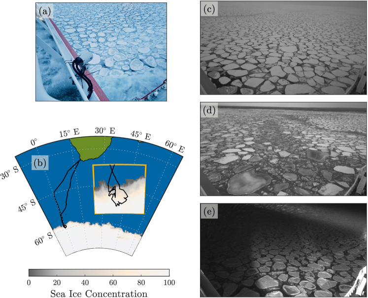
Figure 1: Antarctic SCALE expedition, winter 2022: (a) camera mounted on S.A. Agulhas II; (b) ship’s track; (c) high-resolution image of the sea ice surface obtained under clear sky conditions; (d) exhibiting varying ice gradients; (e) taken at nighttime.

The sensor consisted of a GigE monochrome industrial camera (Fig. 1a) equipped with 2/3” Sony CMOS Pregius sensors and 5 mm F1.8 C-mount lenses (angle of view $\approx$120 degrees). It was mounted on the port side of the monkey bridge at 25 m above the water line and tilted by $\approx$70 degrees relative to the ground. The field of view covered a portion of the ocean surface of $\approx$ 200$\times$200 m². Images were recorded continuously with a resolution of 1920$\times$1080 pixels and at a sampling rate of 1 Hz; around 90,000 images were collected during the expedition. Flashlights were used to illuminate sea ice overnight.

Therefore, the database spans through a wide range of photo quality, with approximately 70% capturing complex ice scenarios. This significant portion includes images taken in the darkness of night or featuring irregularly shaped and densely packed ice floes with varying gradients; sample images are reported in Fig. 1c-e. While many image segmentation methods perform well under ideal conditions, field conditions seldom meet this criterion, presenting a non-uniform and unpredictable environment.

3 Pre-processing

3.1 Orthorectification

The tilt of the sensor produces a perspective distortion, so that ice floes close to the camera appear bigger than those at a farther location. This creates inconsistencies in the scaling, which changes throughout the imagery scene and, hence, compromises the pixel-to-metre conversion. Therefore, a correction process that rectifies the sensor orientation, known as orthorectification, was applied to rearrange the displaced pixels as if the image were aligned with the focal plane (i.e. pixels are projected onto a plane perpendicular to the optical axis).

The process relies on the interpolation of the pixels in the original image as a function of the camera projection matrix, which maps the conversion from a three dimensional point cloud in the real world into a two dimensional plane (the image) through intrinsic and extrinsic parameters (Hartley and Zisserman, 2004). The former depend on how the sensor captures the images and include, but they are not limited to, the focal length, aperture, resolution and the optical center of the camera’s sensor. These parameters were derived from a calibration process (a common method is presented in Zhang, 2000), which evaluated image distortion by analysing multiple images of a planar pattern with known geometry (a chessboard; see technical details in Sturm and Maybank, 1999; Bouguet, 2004). The calibration was performed before and after the expedition to verify that intrinsic features remained constant throughout the campaign. The extrinsic parameters, on the other hand, describe the translations and rotations of the sensor relative to a reference Cartesian coordinate system. For simplicity, the camera was centered at the origin of the horizontal axis, so that translations in the x and y directions were nil, and at a height of 25 m above the water line. The rotations encompass three components: the tilt around the transverse axis, which was applied during deployment; the roll around the optical axis, which was negligible assuming alignment with the horizon; and the heading around the vertical axis, which aligned with the sensor’s direction. The latter is relevant only if the target is a specific object in the field of view, but it becomes negligible if the target is an extended portion of the image (the ocean surface in the present application). In the absence of any external forcing such as the ship motion, translations and rotations are constant over time. A sensitivity analysis relative to ship motion is discussed in §3.2.

The orthorectification was undertaken with the CameraTransfor Python package (Gerum et al., 2019), while the calibration was conducted through the Computer Vision Toolbox for  MatLab (Bouguet, 2004). The process was limited to a portion of the ocean surface confined into a rectangle of about 95 m $\times$ 165 m, which, based on a visual assessment over samples of images, includes clearly visible floes. The resolution (i.e. pixel-to-metre conversion) was forced to 0.05 m, to ensure both a good object accuracy and capacity of determine small-scale features in sea ice (in the order of tens of centimetres; Alberello et al., 2019). A sample image and its orthorectified counterpart are showed in Figure 2.

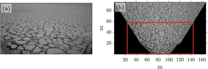
Figure 2: Sample sea ice image (a) from Antarctic SCALE expedition, winter 2022, after perspective correction, with the region of interest for analysis highlighted in red (b).

A quality check after the orthorectification revealed that floe edges loosed sharpness with distance from the sensor (see upper band of Fig. 2b). To avoid ambiguity in the far field and, thus, reduce the risk of detecting unrealistic floes, the workable portion of the orthorectified images was restricted to an area of about 60 m $\times$ 120 m close to the sensors (see area within the red rectangle in Fig. 2b).

3.2 Effect of ship motion

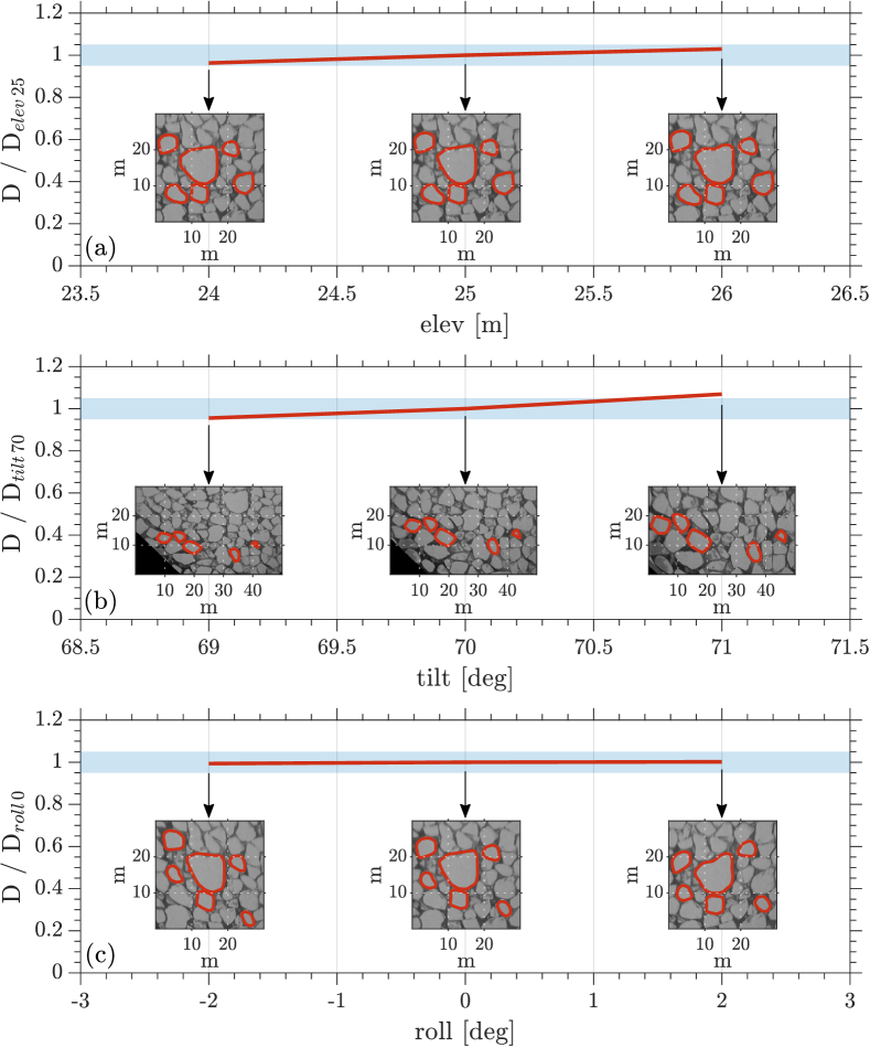
Figure 3: Uncertainty analysis of extrinsic camera parameters on the average diameter of ice floes, highlighted in red. This analysis includes variations of (a) $\pm$ 1 m in elevation, (b) $\pm$ 1 degree in tilt, and (c) $\pm$ 2 degrees in roll. Diameters are normalized with those derived from the image orthorectified using the extrinsics measured aboard the ship. The shaded blue area indicates a 5% range.

The orthorectification, upon which segmentation is based, relies on the positioning of the sensor (the extrinsic parameters). Consistently with similar applications from mobile platforms like aircraft (Parmiggiani et al., 2018; Zhang and Skjetne, 2015) and ships (Alberello et al., 2019; Heyn et al., 2017), it was assumed that the sensor was fixed and, hence, the ship-induced motion was neglected. Although this hypothesis holds under in relatively calm seas, the ship motion was substantial during the expedition (cf. Alberello et al., 2022). As the displacement of the supporting platform can shift the camera’s orientation relative to the ocean surface, it affects the orthorectification and, eventually, the floe size.

An image recorded in clear sky condition is used as a proxy to assess the sensitivity to ship motion. The orthorectification is obtained considering several misalignment relative to the original position, varying $\pm$ 1 m, $\pm$ 1 degrees, and $\pm$ 2 degrees for elevation, tilt and roll, respectively. These ranges are consistent with extreme ship motion recordings. A few clearly distinguishable floes are then manually segmented by meticulously outlining their contours using photo editing software, ensuring accurate comparison of their dimensions.

Figure 3 shows the average variation in size, relative to the dimension extrapolated from the image with sensor in its original position, as a function of the misalignment. Uncertainties associated to variations of elevation are confined within 5% (Fig. 3a). Variations in the tilt result in a slightly more substantial impact on floe size (Fig. 3b), but they only marginally exceed 5%. Changes of roll has the least impact, with variations of size less than 2% (Fig. 3c). It should be noted that the impact of ship motion is evaluated considering elevation, tilt and roll independently. However, they are concurrent during navigation, counteracting each other and so mitigating the overall error, which can be confirmed negligible.

3.3 Image enhancement

Sea ice imagery captured in natural environments suffers from varying light intensity, contrast, shadows, impurities, and other dynamic factors, making segmentation challenging. Within the database, image illumination and contrast varied significantly due to differences in lighting and weather conditions (see Fig. 1c-e). Consequently, the boundaries of ice floes in the raw images often remained uncertain, complicating the automation of segmentation processes (see, for example, Maška et al., 2023).

Image enhancement techniques were applied to sharpen the edges. This was achieved through the homogenization of gray-scale levels (see, for example, Parmiggiani et al., 2018), using a combination of an edge-preserving Gaussian bilateral filter (Tomasi and Manduchi, 1998) and an anisotropic diffusion filter (Perona and Malik, 1990). These filters smoothed regions with low gradients while preserving the boundaries of the ice floes. Contrast enhancement was then applied using contrast-limited adaptive histogram equalization (CLAHE) (Zuiderveld, 1994) to accentuate the boundaries and reveal fine details (see transition from original to enhanced image in Fig. 4a,b). It is worth mentioning that the adaptive nature of this method allows it to tailor its adjustments to the specific characteristics of each image, eliminating the need for predefined thresholds. For night photographs, image enhancement was limited to the area illuminated by the vessel’s spotlight, which was identified through haze removal techniques (He et al., 2011). These techniques were used to estimate the illumination map by inverting the low-light image, applying dehazing, and then reinverting the result, effectively highlighting the spotlight-illuminated areas.

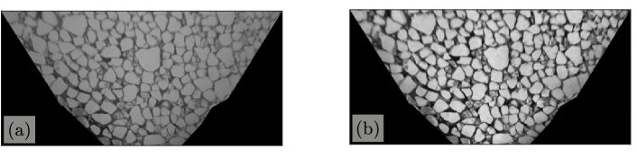
Figure 4: Image enhancement: (a) region of interest of the image in Fig. 2b; (b) gray-level homogenization through Gaussian bilateral and anisotropic diffusion filter, and contrast enhancement using CLAHE;

4 Image segmentation

4.1 Active contours model

Active contour models, or snakes, have proven effective for segmenting connected floes in images (Zhang and Skjetne, 2015), a common occurrence in the Southern Ocean. These models adjust an evolving curve to align with floe boundaries (Kass et al., 1988) (an example of the evolution of an initial contour is presented in the inset of Fig. 5). Their accuracy, however, depends on the initial contour placement. Poor placement may result in incorrect boundaries, while contours placed near the true edges enable faster and more precise convergence. To eliminate the need for manual contouring, an automated contour generator, capable of adapting to various floe shapes, has been introduced, making the segmentation process fully autonomous.

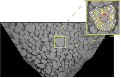
Figure 5: Graphical representation of the Gradient Vector Flow (GVF) algorithm, featuring a dynamic curve that adjusts to precisely conform to the boundaries of the ice floes.

The several steps for the image segmentation are illustrated in Fig. 6. The process starts with the separation of the foreground (i.e. the objects) from the background through the transformation of the enhanced ice image into a binary counterpart (Fig. 6b). This is achieved by selecting an appropriate threshold in the gray-scale histogram of the entire image. Pixels below the threshold are allocated a value of zero and labeled as non-feature pixels (background), while those above it are assigned a value of one and labeled as feature pixels (foreground; this corresponds to the white islands in Fig. 6b). In the presence of many objects with low gray-scale contrast, the histograms does not show distinctive modes necessarily, leaving ambiguities in the selection of appropriate thresholds. To prevent uncertainties, the Otsu method (Otsu, 1979) is used for automated thresholding. Otsu’s method automatically determines the optimal threshold by maximizing the variance between the foreground and background pixel intensities. To further improve accuracy, the binarization is applied on small clusters of size 12 m $\times$ 12 m, each of which contains approximately 20 floes. The smaller size of the clusters produces more segregated modes in the grey-scale histogram, enhancing the effectiveness of automated thresholding (Byun and Nam, 2021).

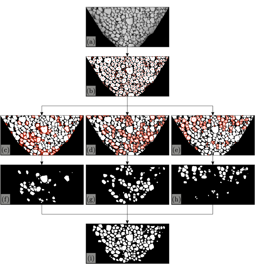
Figure 6: GVF Snake algorithm: (a) enhanced sea ice image; (b) seeds in red of the ice floes in the binary equivalent of the image; (c) perimeter in red of the floes containing a single seed; (d) elliptical initial contour in red of the floes containing a single seed after a morphological erosion; (e) circular initial contour in red for each remaining and unused seed; (f) ice floes already identified in Fig. 6c; (g) ice floes detected by the GVF snake algorithm initialized with the elliptical contours; (h) ice floes detected by the GVF snake algorithm initialized with the circular contours; (i) final binary image with all the detected ice floes.

A distance transformation (Paglieroni, 1992) is then applied to the binary image to assign each feature pixel a value corresponding to its distance from the nearest non-feature pixel (Maurer et al., 2003). The local maxima within this matrix, defined as pixels with values greater than or equal to those of their neighbors, identify seeds that pinpoint individual objects (cf. Zhang and Skjetne, 2015). Similarly to the clustering of binarisation, regional local maxima from sub-regions of the whole image were considered to enhance accuracy. If the portion of image within a sub-region is sharp, objects are well separated and possesses only one seed. Therefore, their segmentation automatically follows from the binarisation. This initial phase of floe detection is reported in Fig. 6c,f, which show seeds and the concurrent segmented objects respectively.

For the majority of sub-regions, however, adjacent objects were merged through the process and thus could not be segmented by binarisation alone. This resulted in large and irregular (white) islands pinpointed by more that one seed (see Fig. 6b). For these cases, the segmentation is achieved through a second phase, which relies on a gradient vector flow (GVF) Snake algorithm (Xu and Prince, 1998). As an extension of traditional active contour models, the GVF Snake is less dependent on the initial contour and, thus, it can process objects with complex shapes more efficiently, even in noisy and low contrast images. The initial contour shape does not restrict the final segmentation from aligning with irregular boundaries. As most of the objects are connected to each others through only a few pixels, they can be isolated by smoothing the edges with a morphological erosion process (Adams, 1993). These newly emerging objects are initialised by ellipses, which represent a natural shape for ice floes (cf. Alberello et al., 2019; Passerotti et al., 2022). The initial contour is selected so that the second moment of the covariance matrix matches the one of the object (Mulchrone and Choudhury, 2004); see Fig. 6d. The unprocessed objects remain within conglomerates of white regions as they share a significant portion of the edge with their neighbors, which cannot be consumed with morphological erosion. Segmentation is achieved by applying circles as initial contours to seeds, noting that the circular shape is an alternative to ellipses for approximating ice floes of small dimensions (Alberello et al., 2019). Relying on the distance transform, the radius is selected such that the contour is within the object, but not too far from the presumed edge (Fig. 6e). Once initial contours are assigned to all seeds, the GVF snake algorithm is applied to expand the contours and, hence, identify the object’s boundaries (Fig. 6g,h). The algorithm requires approximately 30 seconds per floe to complete the segmentation.

The GVF approach is not free from anomalies and inaccuracies, which can result in features that are not present in the original image. Coefficients of circularity and eccentricity are used to quantify how closely the various shape resembles a perfect circle or how much elongated the feature is (see Ayoub, 2003; Bottema, 2000). Through the imposition of high-valued thresholds, spurious features in the form of nearly-perfect circular shapes or line segments are eliminated. Furthermore, objects without closed boundaries at the image’s edges are also disregarded.

The final output of the analysis combines results from the various phases and is reported in Fig. 6i. From this binary mask, geometric properties such as area, perimeter, and diameter are extracted by identifying connected pixel regions corresponding to each floe. Area is calculated from the number of pixels in each region, while perimeter and diameter are determined using boundary tracing techniques (Biswas and Hazra, 2018), which follow the edges of each floe to measure their outlines and maximum span.

4.2 Segment Anything Model

Unlike traditional snake-based models, which rely on pixel-level features such as smoothness, roughness, and contrast specific to each image, modern AI-driven techniques interpret images based on general patterns learned from extensive training datasets. Vision foundation models (Dosovitskiy et al., 2020) exemplify this innovation in image segmentation. By leveraging deep learning techniques, these models process entire images without requiring prior knowledge of an object’s shape, eliminating the need for manual feature engineering or predefined contours.

Segment Anything Model (SAM) (Kirillov et al., 2023), developed by Meta AI Research, stands as the first and only vision foundation model capable, in principle, of segmenting any object in an image. Built on the widely-used PyTorch deep learning framework (Ketkar and Moolayil, 2021), SAM offers two distinct segmentation modes. The first, an automatic mask generator, segments all identifiable elements in an image independently, requiring no input from the user. SAM autonomously determines which areas to segment based on its internal parameters, providing a fully automated solution. The second, a prompt-based mode, allows users to guide the segmentation process by marking regions of interest with points or bounding boxes. This modality is particularly valuable when precision and control over the segmented areas are critical.

4.2.1 Automatic mask generator

In the automatic mask generator mode, SAM autonomously selects a set of sample points from a fixed grid that spans the entire input image (see Fig. 7a for a visual representation of a sample grid layout). For each selected point in the grid, the model generates one or more candidate masks, where pixels associated with identified objects are assigned a value of one (feature pixels), and pixels representing the background are assigned a value of zero (non-feature pixels). SAM then processes these candidate masks to eliminate redundancy by identifying and removing overlapping or duplicate masks. Additionally, it filters the remaining masks for quality, ensuring that only the most accurate and relevant masks are kept. The final output is a list of filtered masks representing all distinct elements in the image that SAM successfully identifies (see Fig. 7b). For a sea ice image, this list includes separate masks for ice floes, interstitial ice, and open water regions. This entire process is fully autonomous, without any need for user input at any stage.

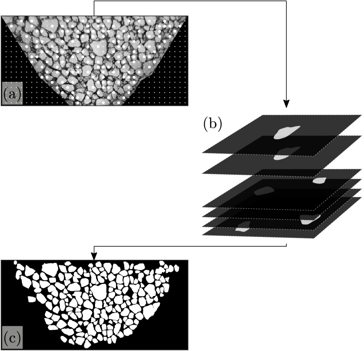
Figure 7: SAM’s automatic mask generator algorithm: (a) fixed points selected by SAM over the grid in the enhanced sea ice image; (b) consolidation of the list of filtered masks returned by the model; (c) final unified mask with all the detected ice floes.

SAM requires post-processing to eliminate anomalies, inaccuracies, and objects with open boundaries at the image’s edges (cf. §4.1). While circularity and eccentricity effectively remove many of these irregularities, they are not sufficient to filter out masks representing open water regions, which are not the target of the sea ice analysis. To resolve this, the convexity coefficient (Sklansky, 1970) is used as an additional filtering criterion. Convexity measures how closely an object’s boundary resembles that of a convex shape; the smoother and more regular the boundary, the closer its convexity value will be to 1. Ice floes, which can often be approximated by ellipses or circles, typically have convexity values near 1. Because the image consists of only ice and water, the surrounding water regions, having more irregular boundaries, naturally exhibit much lower convexity values in comparison. By applying a high convexity threshold, these irrelevant water regions can be easily filtered out (cf. Wang et al., 2024).

A closer examination of the output list reveals that some masks redundantly represent the same ice floes, indicating that the model’s deduplication process is not always optimal. This issue is especially prevalent with adjacent or overlapping floes that have poorly defined boundaries. In such cases, the model may generate multiple identical or overlapping masks for the same floe. If left unresolved, this redundancy makes the output list unsuitable for direct quantitative analysis, as it may lead to the repeated inclusion of the same floe (see first two layers in Fig. 7b). To address this, the masks in the output list are consolidated into a single, unified mask (cf. Shankar et al., 2023). This consolidation performs a union operation, where a pixel is marked as a feature pixel in the final binary mask if it was labeled as a feature pixel in any of the initial masks. This process effectively eliminates redundancy, as multiple occurrences of identical feature pixels in separate masks are included only once in the final mask (see Fig. 7c).

Perimeters and properties of the ice floes segmented by SAM are finally extracted from the comprehensive mask using boundary tracing techniques. It is worth mentioning that the model was run on a consumer CPU, with a runtime of approximately 3 minutes per image. For faster processing, deployment on a GPU is recommended, as its parallel computing capabilities significantly accelerate deep learning.

4.2.2 Prompt-based

In the prompt-based mode, the user provides single or multiple prompts, such as points or bounding boxes, to guide the segmentation process. These prompts can indicate the object or area to segment, or specify both the object and areas to exclude. Since SAM’s prompt-based mode does not apply any automatic filtering, the model segments only the objects explicitly highlighted by the user’s prompts, without further refinement.

Figure 8: SAM’s prompt-based algorithm: (a) seeds in red of the ice floes in the enhanced sea ice image; (b) consolidation of the list of filtered masks returned by the model; (c) final unified mask with all the detected ice floes.

For sea ice images, seeds derived from the distance transform matrix (see description in §4.1 and Fig. 6b) have been found to effectively pinpoint individual ice floes. Each seed is then used as a prompt, which is fed into the model to generate a mask for the corresponding ice floe (Fig. 8a). The output is a list of masks of size n, where n corresponds to the number of seeds in the image. However, when a seed is placed in a region of high uncertainty in the image, the resulting mask may not accurately isolate the intended floe. Instead of containing just the floe, the mask may also erroneously capture unwanted areas, such as discontinuous water regions or parts of adjacent floes (see first two layers in Fig. 8b). The application of the shape-based filters – measuring circularity, eccentricity, and convexity – removes clusters of feature pixels that do not match the typical shape of ice floes, such as water regions. While clusters representing parts of adjacent floes are merged with the correct floe through a union operation during the consolidation process. This operation unifies all the masks in the output list into a single mask, effectively combining the segmented portions of floes into their appropriate masks (Fig. 8c). From this final binary mask, all properties of each individual ice floe can be easily extracted.

SAM is up to 5 times faster when using seeds as prompts compared to the automatic mode and also segments more floes. The prompt-based mode is quicker because it bypasses the model’s internal point selection process, speeding up segmentation. Additionally, in the automatic mode, SAM selects a fixed number of points, which is often insufficient to cover all the ice floes in the image, resulting in fewer floes being segmented.

4.3 A combination of SAM and GVF Snake algorithms

Snake-based models excel at accurately delineating floes but struggle in complex scenarios, such as ice floes with varied gradients, due to their reliance solely on visual characteristics. SAM, on the other hand, benefits from training on extensive and diverse datasets but does not integrate shape details into its segmentation process, leading to issues with adjacent floes that have weak edges. Combining SAM with active contours overcomes these limitations, with the GVF model enhancing SAM’s segmentation by incorporating detailed floe shape information.

Figure 9: SAM-GVF hybrid algorithm: (a) enhanced sea ice image; (b) unified binary mask produced by SAM’s prompt mode with seeds in red of the ice floes; (c) contour in red of the floes containing a single seed because already correctly segmented by SAM; (d) initial contour in red of the floes containing a single seed after a morphological erosion; (e) circular initial contour in red for each remaining and unused seed; (f) ice floes already identified in Fig. 9c; (g) ice floes detected by the GVF snake algorithm initialized with the initial contours in Fig. 9d; (h) ice floes detected by the GVF snake algorithm initialized with the circular contours; (i) final binary image with all the detected ice floes.

The combination of SAM and GVF begins with a broad identification of ice floes using SAM, followed by precise shape-specific refinements with GVF. The steps for this hybrid segmentation approach are shown in Fig. 9. The process starts with SAM’s prompt-based mode applied to the enhanced sea ice image, as outlined in §4.2.2. Seeds from the distance transform matrix (see description in §4.1) are used to initialize SAM, generating masks for individual floes. While this method efficiently isolates floes, it can sometimes produce inaccuracies due to uncertainty in certain areas of the image. To address this, the individual masks are consolidated into a unified binary mask (Fig. 9b). The consolidation corrects segmentation by eliminating uncertain masks and retaining those clearly associated with floes. However, even though most floes are successfully detected and separated, challenges arise when adjacent floes have blurred or unclear edges. The model struggles to accurately assign these ambiguous edge regions to a single floe, causing such floes to be welded together at their unclear boundaries during the mask unification process. This underscores the need for further refinement to distinguish closely adjacent floes that lack clear discontinuity.

The refinement of SAM’s segmentation is achieved through a subsequent phase using the GVF model. In this process, the binary mask used to find the seeds for generating the initial contours is the final output of SAM’s prompt-based mode (Fig. 9b). As a result, most floes are already detected and require no further processing, represented by feature pixel regions pinpointed by only one seed (Fig. 9c). Excluding these floes (Fig. 9f) from the GVF processing reduces computational time and focuses the initial contour placement on the floes SAM did not segment correctly, represented by withe regions with multiple seeds (Fig. 9d,e).

Some of the interconnected objects are linked by only a few pixels and can be separated through morphological erosion, which smooths the edges and isolates the objects. The contours of the newly emerged objects (identifiable as white islands pinpointed by one seed after the erosion) serve as the initial contours for the GVF snake model (see Fig. 9d). These objects represent the ice floes that SAM partially segments, capturing their general shapes but not fully separating them. By using their contours, the shape characteristics of the floes are preserved, enabling the snake model to expand the contours to the true boundaries of each floe.

The remaining unprocessed objects, which share a significant portion of their edges with neighboring objects, cannot be effectively separated using morphological erosion. For these cases, circles are used as initial contours around the seeds – a common approach for approximating ice floes in the marginal ice zone. The radius of each circle is determined by leveraging the distance transform matrix to ensure the contour stays within the object while remaining close to its edge (Fig. 9e). Once all seeds are associated with an initial contour, the GVF snake algorithm is applied to expand these contours and accurately trace the true boundaries of each object (Fig. 9g-h).

The advantage of applying the GVF snake algorithm is its ability to capture the shape of ice floes in densely packed environments where SAM struggles to define boundaries. However, even the combined SAM and GVF approach may introduce anomalies and inaccuracies not present in the original image. As with the standalone GVF application, spurious features such as nearly-perfect circles or elongated line segments are removed using circularity and eccentricity coefficients (see §4.1 for details). The final output, combining results from all phases, is presented in Fig. 9i, from which floe properties are extracted using boundary tracing algorithms.

5 Validation of methods for sea ice analysis

5.1 Creation of benchmark segmentation

In the field of image segmentation, establishing a ground truth dataset is essential as it provides the benchmark for evaluating the performance of automated segmentation algorithms. A ground truth dataset consists of images that have been manually annotated by experts to offer the most accurate and reliable segmentation of objects. These manually segmented results represent the true or correct outputs that automated methods aim to replicate. Such a reference is particularly important in complex environments, such as the Southern Ocean, where segmentation algorithms face challenges due to variable lighting, textures, and scene composition. Without a ground truth as a baseline, it would be difficult, if not impossible, to objectively determine how well these detection algorithms perform.

A robust ground truth was created by manually segmenting a subset of 20 images from the original dataset (refer to §2) that capture diverse visual conditions in the Southern Ocean. These images reflect varying levels of sea ice clarity, deviating from idealized conditions like clear ice boundaries and consistent contrast. The manual segmentation, conducted using Pixelmator on MacOS but compatible with any photo editing software, involved meticulously outlining ice floes to create high-fidelity reference data. This diversity ensures the dataset is representative of the environmental variability. However, it is important to acknowledge that manual segmentation inherently involves some subjectivity, arising not only from individual interpretation but also from the ambiguous definition of what constitutes an ice floe. To mitigate this subjectivity and enhance the benchmark’s robustness, increasing the number of images in the dataset is a practical approach.

The segmented images enable the extraction and analysis of key floe parameters, such as size and concentration. This dataset provides a critical benchmark for accurately evaluating automated detection methods, revealing their strengths and identifying areas for improvement. Without this comparison, the accuracy and reliability of algorithm performance would be uncertain, potentially compromising the validity of quantitative analyses from these image segmentation methods.

5.2 Comparison of floe properties: automated vs. manual segmentation

The automated segmentation methods – GVF, SAM, and the combined SAM-GVF – were applied to the same subset of 20 benchmark images. For each image, key floe properties, such as the number of detected floes, concentration, and size distribution, were extracted. These overall statistics were then compared to those derived from the manual segmentation to assess the accuracy and reliability of each method. The floes parameters comparison is presented in Fig. 10. The upper panel (Fig. 10a-b) displays the number of detected floes and ice concentration, with all values normalized to the manual benchmark. Each black line segment extending from the circles to the horizontal line (representing the manual benchmark at 1) shows how far each method’s results deviate from the benchmark. Shorter lines indicate closer agreement with the manual segmentation. The middle panel (Fig. 10c) shows the floe size distribution based on diameter, with the manual segmentation on the left side as a benchmark for visual comparison. The lower panel (Fig. 10d-g) presents QQ (Quantile-Quantile) plots, comparing the probability density functions (PDFs) of floe diameters at 10% intervals from 10% to 90%. A QQ plot is a graphical tool used to assess whether two datasets follow the same distribution by plotting their quantiles against each other. In these plots, the solid line represents the 1:1 line of equality, where points would align if the automated segmentation results matched the manual benchmark. The closer the data points are to this line, the more similar the automated segmentation is to the manual reference.

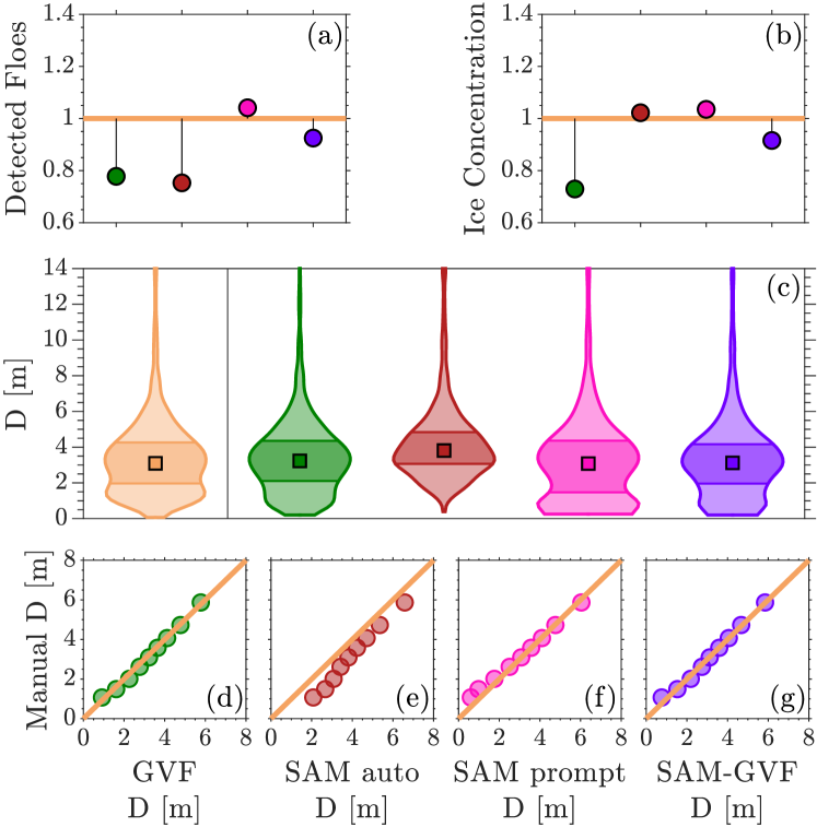
Figure 10: Comparison of floe size statistics obtained through segmentation with GVF (green), SAM automatic (red) and prompt-based (pink) mode, and the combined SAM-GVF (purple) against the manual benchmark (orange) segmentation: (a) number of detected floes for each method, normalized by the corresponding parameter from manual segmentation (horizontal line); (b) ice concentration for each method, normalized by the corresponding parameter from manual segmentation (horizontal line); (c) floe size distribution illustrated as violin plots for all methods, with the manual size distribution shown on the left. Medians and quartiles are represented respectively by squares inside the violins and darker shaded areas; (d-g) QQ plots comparing the quantiles (10% to 90%) of ice floe size distributions derived from the segmentation methods against the benchmark. The solid line indicates the alignment between the method and benchmark quantiles.

Figure 10a shows that the number of floes detected by the automated methods varies when compared to the manual benchmark. GVF and SAM in automatic mode tend to underestimate the number of floes, with values of 0.78 and 0.75, respectively, while SAM in prompt mode tends to overestimate, with a value of 1.05. Despite these discrepancies, the error for this statistic generally stays within 25% of the actual number of floes in the images. The underestimation in both GVF and SAM automatic modes reflects the difficulty these methods face in detecting floes in complex scenarios, such as obscure or irregular ice formations. In SAM’s automatic mode, a fixed number of points are internally selected for initializing the segmentation, which causes the model to prioritize larger, more distinctly detectable floes. As a result, smaller floes or those in more uncertain areas of the image may be overlooked, reducing the total number of segmented floes. On the other hand, the overestimation in SAM prompt mode is due to the model’s tendency to hallucinate, i.e. to generate false contours that resemble floes but do not correspond to any real object in the image. This is particularly common in images with heterogeneous ice gradients or low contrast between ice and water. These false detections are not corrected by the mask consolidation process or by the shape-based filtering described in §4.2.2. The combined GVF-SAM algorithm addresses both underestimation and overestimation issues, resulting in a more accurate floe count, with only a slight underestimation (0.93) of the actual number of floes.

Figure 10b compares sea ice concentration, showing that the SAM-based methods, regardless of the mode, closely match the manual benchmark, with values of 1.02 for the automatic mode and 1.03 for the prompt-based mode. Interestingly, although SAM in automatic mode may struggle to separate adjacent floes with poorly defined edges or overlapping floes – affecting the floe count – it excels at distinguishing between ice and water, leading to high accuracy in estimating the overall sea ice fraction. The combined SAM-GVF method (0.92) has an error range of about 10%, introducing slightly more uncertainty than SAM alone. However, it still outperforms the GVF method (0.73), which tends to under-detect floes or produce contours smaller than the actual floe boundaries, especially when the gradient across the ice floes is not uniform. This limitation causes GVF to underestimate ice concentration, highlighting the benefit of combining it with SAM.

Figure 10c illustrates the floe size distribution using violin plots, which combine elements of box plots and probability density functions. Violin plots show the distribution of data, including the density of values at different points, and provide information on the median (squares inside the violins) and the first and third quartiles (darker shaded areas). In the benchmark, the size distribution is bimodal, with peaks around 2 meters and 4 meters in floe diameter. Fifty percent of the floe sizes fall between 2 and 4.3 meters, with a median of 3 meters. Both the GVF and SAM-GVF methods capture the overall shape of the distribution, including the median and quartiles. The median is slightly overestimated (3.2 meters for GVF and 3.1 meters for SAM-GVF), but the quartiles match the benchmark. Minor discrepancies arise due to the lower detection of smaller floes, preventing accurate capture of the peak at smaller sizes. The SAM distribution varies significantly depending on the mode used. The prompt-based SAM approach closely aligns with the benchmark in terms of median (3 meters) and quartiles, though Q1 is underestimated at 1.6 meters. While the bimodality is captured, there is a skew towards smaller floes (around 1 meter), exaggerating the distribution’s shape compared to the benchmark. The automatic SAM mode, on the other hand, produces the least accurate distribution. Its median is overestimated at 3.8 meters, and the distribution appears unimodal (peaking around 3.5 meters), failing to reflect the bimodal nature of the benchmark. Quartiles are also poorly represented, highlighting the limitations of the automated SAM approach in accurately detecting individual floes without seed-based prompts.

Figure 10d-g present QQ plots, which compare the quantiles of the PDF of the automated methods against the benchmark. The 1:1 line in the plots represents perfect agreement between the two distributions; points lying on this line indicate that the automated method’s distribution matches the benchmark exactly. Deviations from this line highlight differences between the distributions, helping to identify where the automated methods deviate from the manual segmentation. In Fig. 10d, the GVF method shows reasonable agreement with the benchmark, particularly for floe sizes between 2 and 6 meters, where most floes are concentrated. Beyond the lower tails, the data points are fairly close to the 1:1 line, indicating a good match with the benchmark for larger floes. However, in the first 30% of the distribution (corresponding to smaller floes), the data points deviate from the benchmark, suggesting that GVF struggles to accurately detect smaller floes. The root mean square error (RMSE) for this method is 0.14 meters. In contrast, SAM in automatic mode (Fig. 10e) exhibits a more significant difference from the benchmark, as already observed in the previous panel. For this method, the first 50% of floes range between 0 and 3.8 meters, whereas the benchmark ranges from 0 to 3 meters. The quantiles do not follow the 1:1 line, reflecting the deviation in the distribution and the unimodality of SAM automatic mode compared to the bimodality of the benchmark. The RMSE for SAM automatic mode is 0.85 meters. Figures 10f,g display the QQ plots for SAM prompt mode and SAM-GVF, respectively, both of which show similar distributions. The 10% quantile for both methods is around 0.6 meters, compared to 1 meter for the benchmark. This suggests that both methods detect a large number of very small floes not present in the original image, likely corresponding to noise or spurious features that were not filtered out. The 20% and 30% quantiles in SAM prompt mode indicate that the peak towards smaller floes is more pronounced than in the benchmark. Despite this, the rest of the distribution aligns well with the benchmark for both SAM prompt mode and SAM-GVF. The RMSE for SAM-GVF is around 0.13 meters, similar to GVF, whereas the RMSE for SAM prompt mode is 0.25 meters. These values represent the average deviation in the size of floes extracted by the automated methods compared to the manual benchmark. It is important to note that the pixel-to-meter conversion during orthorectification was set to 0.05 meters, meaning the RMSE values for these methods are only 3 to 5 times the smallest measurable unit in the images.

6 Conclusion

The most challenging task in analyzing sea-ice images of the Antarctic marginal ice zone (MIZ) is identifying individual ice floes, especially when boundaries are poorly defined due to variable ice and lighting conditions. In this study, local-scale ice images acquired from the icebreaker S.A. Agulhas II were segmented following three different approaches: the traditional GVF snake method, the modern deep learning technique SAM by Meta, and a hybrid approach combining SAM and GVF. To optimize the images for segmentation analysis, an automated image pre-processing pipeline was developed, which includes orthorectification to correct image distortions and enable pixel-to-meter conversion, as well as image quality enhancement. From the original dataset, 20 images representing the MIZ under varying lighting, weather, and ice conditions were selected and manually segmented to create a benchmark for comparing the performance of the different methods. Quantitative differences in floe size, ice concentration, and the number of correctly identified floes were evaluated against this benchmark.

The analysis reveals that the GVF method is not the most accurate among the tested segmentation approaches when considering the resulting ice concentration and number of floes detected. However, the floe size distribution obtained fairly matches the benchmark. Combining GVF with SAM allows to improve the ice concentration estimates and floe detection, while maintaining accuracy in the size distribution. SAM-GVF produces the floe size distribution most closely aligned with the benchmark, with the lowest RMSE. The segmentation through SAM automatic mode identifies the lowest number of floes in the image and leads to the least accurate size distribution. Despite this, it outperforms the other approaches when considering the resulting sea ice concentration. For this parameter a similar result is obtained when using prompt-based SAM. This mode also improves floe detection and captures the bimodality of the benchmark size distribution more clearly than the other methods.

Declaring one method as superior to another in absolute terms is not possible, as the choice depends on the specific use case. SAM in prompt mode and the hybrid SAM-GVF approach emerged as the most effective overall. Prompt-based SAM, with its faster computational speed and strong performance in estimating ice concentration and detecting floes, is better suited for real-time applications where immediacy is critical. In contrast, the hybrid SAM-GVF approach, along with GVF alone, proved more effective at capturing the floe size distribution. However, their longer computational time makes them more suitable for post-processing and further data refinement.

The growing reliability and applicability of these automated segmentation methods, coupled with rapid advancements in AI, will increasingly enable long-term and real-time observation of sea ice dynamics, revolutionizing our ability to monitor and predict changes in the critical polar regions.

References

- Herman et al. [2021] Agnieszka Herman, Marta Wenta, and Sukun Cheng. Sizes and shapes of sea ice floes broken by waves–a case study from the east antarctic coast. Frontiers in Earth Science, 9, May 2021. ISSN 2296-6463. doi:10.3389/feart.2021.655977.
- Dolatshah et al. [2018] A. Dolatshah, F. Nelli, L. G. Bennetts, A. Alberello, M. H. Meylan, J. P. Monty, and A. Toffoli. Letter: Hydroelastic interactions between water waves and floating freshwater ice. Physics of Fluids, 30(9), September 2018. ISSN 1089-7666. doi:10.1063/1.5050262.
- Montiel et al. [2016] Fabien Montiel, V. A. Squire, and L. G. Bennetts. Attenuation and directional spreading of ocean wave spectra in the marginal ice zone. Journal of Fluid Mechanics, 790:492–522, February 2016. ISSN 1469-7645. doi:10.1017/jfm.2016.21.
- Meylan et al. [2021] Michael H. Meylan, Christopher Horvat, Cecilia M. Bitz, and Luke G. Bennetts. A floe size dependent scattering model in two- and three-dimensions for wave attenuation by ice floes. Ocean Modelling, 161:101779, May 2021. ISSN 1463-5003. doi:10.1016/j.ocemod.2021.101779.
- Passerotti et al. [2022] Giulio Passerotti, Luke G. Bennetts, Franz von Bock und Polach, Alberto Alberello, Otto Puolakka, Azam Dolatshah, Jaak Monbaliu, and Alessandro Toffoli. Interactions between irregular wave fields and sea ice: A physical model for wave attenuation and ice breakup in an ice tank. Journal of Physical Oceanography, 52(7):1431–1446, July 2022. ISSN 1520-0485. doi:10.1175/jpo-d-21-0238.1.
- Horvat et al. [2016] Christopher Horvat, Eli Tziperman, and Jean-Michel Campin. Interaction of sea ice floe size, ocean eddies, and sea ice melting. Geophysical Research Letters, 43(15):8083–8090, August 2016. ISSN 1944-8007. doi:10.1002/2016gl069742.
- Tsamados et al. [2014] Michel Tsamados, Daniel L. Feltham, David Schroeder, Daniela Flocco, Sinead L. Farrell, Nathan Kurtz, Seymour W. Laxon, and Sheldon Bacon. Impact of variable atmospheric and oceanic form drag on simulations of arctic sea ice*. Journal of Physical Oceanography, 44(5):1329–1353, April 2014. ISSN 1520-0485. doi:10.1175/jpo-d-13-0215.1.
- Lüpkes et al. [2012] Christof Lüpkes, Vladimir M. Gryanik, Jörg Hartmann, and Edgar L. Andreas. A parametrization, based on sea ice morphology, of the neutral atmospheric drag coefficients for weather prediction and climate models. Journal of Geophysical Research: Atmospheres, 117(D13), July 2012. ISSN 0148-0227. doi:10.1029/2012jd017630.
- Feltham [2005] Daniel L Feltham. Granular flow in the marginal ice zone. Philosophical Transactions of the Royal Society A: Mathematical, Physical and Engineering Sciences, 363(1832):1677–1700, July 2005. ISSN 1471-2962. doi:10.1098/rsta.2005.1601.
- WORBY [2004] A WORBY. Studies of the antarctic sea ice edge and ice extent from satellite and ship observations. Remote Sensing of Environment, 92(1):98–111, July 2004. ISSN 0034-4257. doi:10.1016/j.rse.2004.05.007.
- Hepworth et al. [2020] Ehlke Hepworth, Marcello Vichi, Armand van Zuydam, Nicole Catherine Taylor, Jesslyn Bossau, Martinique Engelbrecht, and Tor Aarskog. Sea ice observations in the antarctic marginal ice zone during winter 2019, 2020.
- Sandru et al. [2020] Andrei Sandru, Heikki Hyyti, Arto Visala, and Pentti Kujala. A complete process for shipborne sea-ice field analysis using machine vision. IFAC-PapersOnLine, 53(2):14539–14545, 2020. ISSN 2405-8963. doi:10.1016/j.ifacol.2020.12.1458.
- Zhang and Skjetne [2015] Qin Zhang and Roger Skjetne. Image processing for identification of sea-ice floes and the floe size distributions. IEEE Transactions on Geoscience and Remote Sensing, 53(5):2913–2924, May 2015. ISSN 1558-0644. doi:10.1109/tgrs.2014.2366640.
- Alberello et al. [2019] Alberto Alberello, Miguel Onorato, Luke Bennetts, Marcello Vichi, Clare Eayrs, Keith MacHutchon, and Alessandro Toffoli. Brief communication: Pancake ice floe size distribution during the winter expansion of the antarctic marginal ice zone. The Cryosphere, 13(1):41–48, January 2019. ISSN 1994-0424. doi:10.5194/tc-13-41-2019.
- Parmiggiani et al. [2018] F. Parmiggiani, M. Moctezuma-Flores, P. Wadhams, and G. Aulicino. Image processing for pancake ice detection and size distribution computation. International Journal of Remote Sensing, 40(9):3368–3383, November 2018. ISSN 1366-5901. doi:10.1080/01431161.2018.1541367.
- Weissling et al. [2009] B. Weissling, S. Ackley, P. Wagner, and H. Xie. Eiscam — digital image acquisition and processing for sea ice parameters from ships. Cold Regions Science and Technology, 57(1):49–60, June 2009. ISSN 0165-232X. doi:10.1016/j.coldregions.2009.01.001.
- Alsharay et al. [2022] Nahed M. Alsharay, Yuanzhu Chen, Octavia A. Dobre, and Oscar De Silva. Improved sea-ice identification using semantic segmentation with raindrop removal. IEEE Access, 10:21599–21607, 2022. ISSN 2169-3536. doi:10.1109/access.2022.3150969.
- Lu et al. [2016] Wenjun Lu, Qin Zhang, Raed Lubbad, Sveinung Løset, and Roger Skjetne. A shipborne measurement system to acquire sea ice thickness and concentration at engineering scale. In All Days, 16OARC. OTC, October 2016. doi:10.4043/27361-ms.
- Heyn et al. [2017] Hans-Martin Heyn, Martin Knoche, Qin Zhang, and Roger Skjetne. A system for automated vision-based sea-ice concentration detection and floe-size distribution indication from an icebreaker. In Volume 8: Polar and Arctic Sciences and Technology; Petroleum Technology, OMAE2017. American Society of Mechanical Engineers, June 2017. doi:10.1115/omae2017-61822.
- Lu et al. [2008] P. Lu, Z. J. Li, Z. H. Zhang, and X. L. Dong. Aerial observations of floe size distribution in the marginal ice zone of summer prydz bay. Journal of Geophysical Research: Oceans, 113(C2), February 2008. ISSN 0148-0227. doi:10.1029/2006jc003965.
- Dumas-Lefebvre and Dumont [2023] Elie Dumas-Lefebvre and Dany Dumont. Aerial observations of sea ice breakup by ship waves. The Cryosphere, 17(2):827–842, February 2023. ISSN 1994-0424. doi:10.5194/tc-17-827-2023.
- Zhang et al. [2022] Chengqian Zhang, Xiaodong Chen, and Shunying Ji. Semantic image segmentation for sea ice parameters recognition using deep convolutional neural networks. International Journal of Applied Earth Observation and Geoinformation, 112:102885, August 2022. ISSN 1569-8432. doi:10.1016/j.jag.2022.102885.
- Panchi et al. [2021] Nabil Panchi, Ekaterina Kim, and Anirban Bhattacharyya. Supplementing remote sensing of ice: Deep learning-based image segmentation system for automatic detection and localization of sea-ice formations from close-range optical images. IEEE Sensors Journal, 21(16):18004–18019, August 2021. ISSN 2379-9153. doi:10.1109/jsen.2021.3084556.
- Dowden et al. [2021] Benjamin Dowden, Oscar De Silva, Weimin Huang, and Dan Oldford. Sea ice classification via deep neural network semantic segmentation. IEEE Sensors Journal, 21(10):11879–11888, May 2021. ISSN 2379-9153. doi:10.1109/jsen.2020.3031475.
- Maška et al. [2023] Martin Maška, Vladimír Ulman, Pablo Delgado-Rodriguez, Estibaliz Gómez-de Mariscal, Tereza Nečasová, Fidel A. Guerrero Peña, Tsang Ing Ren, Elliot M. Meyerowitz, Tim Scherr, Katharina Löffler, Ralf Mikut, Tianqi Guo, Yin Wang, Jan P. Allebach, Rina Bao, Noor M. Al-Shakarji, Gani Rahmon, Imad Eddine Toubal, Kannappan Palaniappan, Filip Lux, Petr Matula, Ko Sugawara, Klas E. G. Magnusson, Layton Aho, Andrew R. Cohen, Assaf Arbelle, Tal Ben-Haim, Tammy Riklin Raviv, Fabian Isensee, Paul F. Jäger, Klaus H. Maier-Hein, Yanming Zhu, Cristina Ederra, Ainhoa Urbiola, Erik Meijering, Alexandre Cunha, Arrate Muñoz-Barrutia, Michal Kozubek, and Carlos Ortiz-de Solórzano. The cell tracking challenge: 10 years of objective benchmarking. Nature Methods, 20(7):1010–1020, May 2023. ISSN 1548-7105. doi:10.1038/s41592-023-01879-y.
- Dosovitskiy et al. [2020] Alexey Dosovitskiy, Lucas Beyer, Alexander Kolesnikov, Dirk Weissenborn, Xiaohua Zhai, Thomas Unterthiner, Mostafa Dehghani, Matthias Minderer, Georg Heigold, Sylvain Gelly, Jakob Uszkoreit, and Neil Houlsby. An image is worth 16x16 words: Transformers for image recognition at scale, 2020.
- Raghu et al. [2021] Maithra Raghu, Thomas Unterthiner, Simon Kornblith, Chiyuan Zhang, and Alexey Dosovitskiy. Do vision transformers see like convolutional neural networks?, 2021.
- Kirillov et al. [2023] Alexander Kirillov, Eric Mintun, Nikhila Ravi, Hanzi Mao, Chloe Rolland, Laura Gustafson, Tete Xiao, Spencer Whitehead, Alexander C. Berg, Wan-Yen Lo, Piotr Dollár, and Ross Girshick. Segment anything, 2023.
- Shankar et al. [2023] Siddharth Shankar, Leigh A. Stearns, and C. J. van der Veen. Semantic segmentation of glaciological features across multiple remote sensing platforms with the segment anything model (sam). Journal of Glaciology, pages 1–10, November 2023. ISSN 1727-5652. doi:10.1017/jog.2023.95.
- Ma and Wang [2023] Jun Ma and Bo Wang. Towards foundation models of biological image segmentation. Nature Methods, 20(7):953–955, July 2023. ISSN 1548-7105. doi:10.1038/s41592-023-01885-0.
- Ryan-Keogh and Vichi [2022] Thomas Ryan-Keogh and Marcello Vichi. Scale-win19 & scale-spr19 cruise report, 2022.
- Tersigni et al. [2023] Ippolita Tersigni, Alberto Alberello, Gabriele Messori, Marcello Vichi, Miguel Onorato, and Alessandro Toffoli. High-resolution thermal imaging in the antarctic marginal ice zone: Skin temperature heterogeneity and effects on heat fluxes. Earth and Space Science, 10(9), September 2023. ISSN 2333-5084. doi:10.1029/2023ea003078.
- Hartley and Zisserman [2004] Richard Hartley and Andrew Zisserman. Multiple View Geometry in Computer Vision. Cambridge University Press, March 2004. ISBN 9780511811685. doi:10.1017/cbo9780511811685.
- Zhang [2000] Z. Zhang. A flexible new technique for camera calibration. IEEE Transactions on Pattern Analysis and Machine Intelligence, 22(11):1330–1334, 2000. ISSN 0162-8828. doi:10.1109/34.888718.
- Sturm and Maybank [1999] P.F. Sturm and S.J. Maybank. On plane-based camera calibration: A general algorithm, singularities, applications. In Proceedings. 1999 IEEE Computer Society Conference on Computer Vision and Pattern Recognition (Cat. No PR00149), CVPR-99. IEEE Comput. Soc, 1999. doi:10.1109/cvpr.1999.786974.
- Bouguet [2004] Jean-Yves Bouguet. Camera calibration toolbox for matlab. http://www. vision. caltech. edu/bouguetj/calib_doc/, 2004.
- Gerum et al. [2019] Richard C. Gerum, Sebastian Richter, Alexander Winterl, Christoph Mark, Ben Fabry, Céline Le Bohec, and Daniel P. Zitterbart. Cameratransform: A python package for perspective corrections and image mapping. SoftwareX, 10:100333, July 2019. ISSN 2352-7110. doi:10.1016/j.softx.2019.100333.
- Alberello et al. [2022] Alberto Alberello, Luke G. Bennetts, Miguel Onorato, Marcello Vichi, Keith MacHutchon, Clare Eayrs, Butteur Ntamba Ntamba, Alvise Benetazzo, Filippo Bergamasco, Filippo Nelli, Rohinee Pattani, Hans Clarke, Ippolita Tersigni, and Alessandro Toffoli. Three-dimensional imaging of waves and floes in the marginal ice zone during a cyclone. Nature Communications, 13(1), August 2022. ISSN 2041-1723. doi:10.1038/s41467-022-32036-2.
- Tomasi and Manduchi [1998] C. Tomasi and R. Manduchi. Bilateral filtering for gray and color images. In Sixth International Conference on Computer Vision (IEEE Cat. No.98CH36271), ICCV-98. Narosa Publishing House, 1998. doi:10.1109/iccv.1998.710815.
- Perona and Malik [1990] P. Perona and J. Malik. Scale-space and edge detection using anisotropic diffusion. IEEE Transactions on Pattern Analysis and Machine Intelligence, 12(7):629–639, July 1990. ISSN 0162-8828. doi:10.1109/34.56205.
- Zuiderveld [1994] Karel Zuiderveld. Contrast Limited Adaptive Histogram Equalization, pages 474–485. Elsevier, 1994. doi:10.1016/b978-0-12-336156-1.50061-6.
- He et al. [2011] Kaiming He, Jian Sun, and Xiaoou Tang. Single image haze removal using dark channel prior. IEEE Transactions on Pattern Analysis and Machine Intelligence, 33(12):2341–2353, December 2011. ISSN 2160-9292. doi:10.1109/tpami.2010.168.
- Kass et al. [1988] Michael Kass, Andrew Witkin, and Demetri Terzopoulos. Snakes: Active contour models. International Journal of Computer Vision, 1(4):321–331, January 1988. ISSN 1573-1405. doi:10.1007/bf00133570.
- Otsu [1979] Nobuyuki Otsu. A threshold selection method from gray-level histograms. IEEE Transactions on Systems, Man, and Cybernetics, 9(1):62–66, January 1979. ISSN 2168-2909. doi:10.1109/tsmc.1979.4310076.
- Byun and Nam [2021] Seok-Ho Byun and Jong-Ho Nam. Estimation of pack ice concentration using histogram peak analysis and image subdivision. Cold Regions Science and Technology, 181:103185, January 2021. ISSN 0165-232X. doi:10.1016/j.coldregions.2020.103185.
- Paglieroni [1992] David W Paglieroni. Distance transforms: Properties and machine vision applications. CVGIP: Graphical Models and Image Processing, 54(1):56–74, January 1992. ISSN 1049-9652. doi:10.1016/1049-9652(92)90034-u.
- Maurer et al. [2003] C.R. Maurer, Rensheng Qi, and V. Raghavan. A linear time algorithm for computing exact euclidean distance transforms of binary images in arbitrary dimensions. IEEE Transactions on Pattern Analysis and Machine Intelligence, 25(2):265–270, February 2003. ISSN 0162-8828. doi:10.1109/tpami.2003.1177156.
- Xu and Prince [1998] Chenyang Xu and J.L. Prince. Snakes, shapes, and gradient vector flow. IEEE Transactions on Image Processing, 7(3):359–369, March 1998. ISSN 1057-7149. doi:10.1109/83.661186.
- Adams [1993] R. Adams. Radial decomposition of disks and spheres. CVGIP: Graphical Models and Image Processing, 55(5):325–332, September 1993. ISSN 1049-9652. doi:10.1006/cgip.1993.1024.
- Mulchrone and Choudhury [2004] Kieran F. Mulchrone and Kingshuk Roy Choudhury. Fitting an ellipse to an arbitrary shape: implications for strain analysis. Journal of Structural Geology, 26(1):143–153, January 2004. ISSN 0191-8141. doi:10.1016/s0191-8141(03)00093-2.
- Ayoub [2003] Ayoub B. Ayoub. The eccentricity of a conic section. The College Mathematics Journal, 34(2):116–121, March 2003. ISSN 1931-1346. doi:10.1080/07468342.2003.11921994.
- Bottema [2000] M.J. Bottema. Circularity of objects in images. In 2000 IEEE International Conference on Acoustics, Speech, and Signal Processing. Proceedings (Cat. No.00CH37100), ICASSP-00. IEEE, 2000. doi:10.1109/icassp.2000.859286.
- Biswas and Hazra [2018] Soumen Biswas and Ranjay Hazra. Robust edge detection based on modified moore-neighbor. Optik, 168:931–943, September 2018. ISSN 0030-4026. doi:10.1016/j.ijleo.2018.05.011.
- Ketkar and Moolayil [2021] Nikhil Ketkar and Jojo Moolayil. Introduction to PyTorch, pages 27–91. Apress, 2021. ISBN 9781484253649. doi:10.1007/978-1-4842-5364-9_2.
- Sklansky [1970] J. Sklansky. Recognition of convex blobs. Pattern Recognition, 2(1):3–10, January 1970. ISSN 0031-3203. doi:10.1016/0031-3203(70)90037-3.
- Wang et al. [2024] A. Wang, B. Wei, J. Sui, J. Wang, N. Xu, and G. Hao. Integrating a data-driven classifier and shape-modulated segmentation for sea-ice floe extraction. International Journal of Applied Earth Observation and Geoinformation, 128:103726, April 2024. ISSN 1569-8432. doi:10.1016/j.jag.2024.103726.