SaRA: High-Efficient Diffusion Model
Fine-tuning with Progressive
Sparse Low-Rank Adaptation

Abstract

In recent years, the development of diffusion models has led to significant progress in image, video, and 3D generation tasks, with pre-trained models like the Stable Diffusion series playing a crucial role. However, a key challenge remains in downstream task applications: how to effectively and efficiently adapt pre-trained diffusion models to new tasks. Inspired by model pruning which lightens large pre-trained models by removing unimportant parameters, we propose a novel model fine-tuning method to make full use of these ineffective parameters and enable the pre-trained model with new task-specified capabilities. In this work, we first investigate the importance of parameters in pre-trained diffusion models (Stable Diffusion 1.5, 2.0, and 3.0), and discover that the smallest 10% to 20% of parameters by absolute values do not contribute to the generation process due to training instabilities rather than inherent model properties. Based on this observation, we propose a fine-tuning method termed SaRA that re-utilizes these temporatily ineffective parameters, equating to optimizing a sparse weight matrix to learn the task-specific knowledge. To mitigate potential overfitting, we propose a nuclear-norm-based low-rank sparse training scheme for efficient fine-tuning. Furthermore, we design a new progressive parameter adjustment strategy to make full use of the re-trained / finetuned parameters. Finally, we propose a novel unstructural backpropagation strategy, which significantly reduces memory costs during fine-tuning and further enhances the selective PEFT field. Our method enhances the generative capabilities of pre-trained models in downstream applications and outperforms traditional fine-tuning methods like LoRA in maintaining model’s generalization ability. We validate our approach through fine-tuning experiments on SD 1.5, SD 2.0, and SD 3.0, demonstrating significant improvements. Additionally, we compare our method against previous fine-tuning approaches in various downstream tasks, including domain transfer, customization, image editing, and 3D generation, proving its effectiveness and generalization performance. SaRA also offers a practical advantage that requires only a single line of code modification for efficient implementation and is seamlessly compatible with existing methods. Source code is available at https://sjtuplayer.github.io/projects/SaRA.

1 Introduction

In recent years, with the development of diffusion models (Ho et al., 2020; Rombach et al., 2022), tasks such as image generation (Van Le et al., 2023; Zhang et al., 2023a), video generation (Guo et al., 2023; Blattmann et al., 2023), and 3D generation (Poole et al., 2022; Sun et al., 2023) have made significant advancements. Pre-trained diffusion models, particularly the Stable Diffusion series (Rombach et al., 2022), have played a crucial role in these developments, including image customization (Van Le et al., 2023), image editing (Kawar et al., 2023), and controllable generation (Zhang et al., 2023a; Mou et al., 2024). Additionally, by leveraging prior information from the image domain, diffusion models have been extended to tasks such as video (Guo et al., 2023; Blattmann et al., 2023) and 3D generation (Poole et al., 2022; Sun et al., 2023). As these applications continue to evolve, a core issue emerges: how to effectively and efficiently fine-tune the foundational pre-trained diffusion models and apply them to new tasks.

Existing fine-tuning methods (Han et al., 2024) can be categorized into three categories (Fig. 1): 1) Additive fine-tuning (AFT) methods (Chen et al., 2022), which introduce additional modules to fine-tune the model, such as adapter-based tuning (Ye et al., 2023; Mou et al., 2024). However, these methods require additional modules and parameters, which has changed the source model, and also introduced additional latency during the inference stage. 2) Reparameterized fine-tuning (RFT) methods (Hu et al., 2021; Zhang et al., 2023b), which primarily utilize low-rank matrices to learn new information and merge the learned parameters with the pre-trained one, but it still suffers from the risk of overfitting, since all parameters are adjusted by the low-rank matrices globally. Moreover, the choice of rank and the specific layers to which LoRA is applied requires a tailored design for each model. 3) Selective-based fine-tuning (SFT) methods (Guo et al., 2020; Ansell et al., 2021), which select a subset of the model’s existing parameters for fine-tuning. However, the complex parameter selection process and high memory cost restrict their application in diffusion models. Overall, both AFT and RFT methods require model-specific designs, e.g., exploration of which layers to apply Adapters or LoRAs within the model, and the hidden dimension or rank needs to be adjusted according to the specific tasks. And the SFT method introduces considerable latency, suffers from hyperparameter sensitivity in parameter selection, and also performs poorly in terms of effectiveness and training efficiency. Therefore, a pressing question arises: Can we design a universal method that is model-agnostic, does not require hyperparameter searching, inherently avoids overfitting, and simultaneously achieves high-efficiency plug-and-play model fine-tuning?

Inspired by a theory in model pruning, which posits that within a trained model, there exist parameters with relatively small absolute values that have negligible impact on the model’s output, an intuitive idea is: whether we can find a way to leverage these ineffective parameters to make them effective again, and enhance the model’s generative capabilities. To achieve this goal, the target “ineffective” parameters we seek must possess two properties: 1) temporary ineffectiveness: the parameters themselves have minimal impact on the current model’s output; 2) potential effectiveness: the parameters are not redundant due to the model’s structural design, but have a certain ability to learn new knowledge (if handled properly, they can be effective again). We first conducted an analysis on the influence of small parameters in pre-trained diffusion models (Stable Diffusion 1.5, 2.0, and 3.0) on the model outputs, and found that the smallest $10\%$ (even $20\%$) of parameters by absolute values did not contribute much to the generative process (Fig. 2, see Sec. 3.1). Furthermore, we examined the potential effectiveness of these parameters and discovered that their ineffectiveness is not inherent (extrinsic) to the model’s nature, but rather due to the instability of the training process (see Sec. 3.2). Specifically, the randomness in the training process causes some parameters to approach zero by the end of training. This observation inspired us to rationally utilize these temporally ineffective parameters to make them effective again and fine-tune pre-trained generative models.

Figure 1: The comparison between our SaRA (d) and the previous parameter efficient finetuning methods, including (a) addictive fine-tuning (ATF) (Chen et al., 2022), (b) reparameterized fine-tuning (RFT) (Hu et al., 2021), and (c) the selective fine-tuning (SFT) (Guo et al., 2020). RFT methods address the additional inference latency introduced by ATF methods through reparameterizing the pre-trained weights from a global view. SFT methods improve upon global parameter updates by employing sparse updates, which better preserve the model prior by freezing most of the pre-trained parameters. Our SaRA method further enhances SFT by significantly reducing memory costs and achieving superior performance in both adaptation capability and prior preservation.

Specifically, we propose SaRA, a novel fine-tuning method for pre-trained diffusion models that trains the parameters with relatively small absolute values. We first identify the “temporally ineffective, potentially effective” parameters as paramters smaller than a threshold in the pre-trained weights. We then efficiently fine-tune these parameters in the pre-trained weights by sparse matrices while preserving prior knowledge. To mitigate the risk of overfitting due to the potential high rank of sparse matrices, we propose a low-rank sparse training scheme, which employs a nuclear norm-based low-rank loss to constrain the rank of the learned sparse matrices, achieving efficient fine-tuning of diffusion models. In addition, recognizing that some parameters may not be fully utilized during the fine-tuning process, we propose a progressive parameter adjustment strategy, which introduces a second stage to reselect parameters below the pre-defined threshold and train them, ensuring that almost all parameters contribute effectively. Finally, different from the typical selective PEFT methods that retain the gradient of the entire parameter matrices and require high memory cost (the same as full-parameter fine-tuning), we propose an unstructural backpropagation strategy with smaller memory cost. In this strategy, we only retain the gradients for the parameters to be updated, and automatically discard the gradients for other parameters during the backpropagation process. This results in a memory-efficient selective PEFT method, which also advances the development of future selective PEFT techniques.

Compared to previous fine-tuning methods (Hu et al., 2021; Valipour et al., 2022; Hayou et al., 2024), our SaRA is capable of effectively enhancing the generative capabilities of the pre-trained model itself, which improves around 5% performance of Stable Diffusion models pre-trained on ImageNet (Deng et al., 2009), CelebA-HQ (Karras et al., 2017) and FFHQ (Karras et al., 2019) dataset (see Sec. 5.2). Moreover, we employ our SaRA to fine-tune Stable Diffusion 1.5, 2.0, and 3.0 on five downstream datasets with different number of trainable parameters (5M, 20M, and 50M), achieving the best FID score and balance both the FID and CLIP score better than the other PEFT methods, along with full fine-tuning method (see Sec. 5.3). Furthermore, we compare our method with previous fine-tuning methods across multiple downstream tasks, including image customization, and controllable video generation, demonstrating the effectiveness of our approach in different generation tasks (see Sec. 5.4). Moreover, we encapsulated and implemented our method to allow model fine-tuning with just a single line of code modification in the original training script, which significantly enhances the ease of use and adaptability of the code for other models and tasks.

Contributions of this paper can be summarized in the following four aspects:

• We investigate the importance of the parameters in pre-trained diffusion models, revealing the temporal ineffectiveness and potential effectiveness of the parameters with the smallest absolute weight, which motivates us to make full use of these parameters.

• We propose SaRA, a novel efficient fine-tuning method based on progressive sparse low-rank adaptation, where a nuclear-norm-based low-rank loss is employed to effectively prevent model overfitting, and a progressive training strategy is introduced to make full use of the ineffective parameters, therefore enabling the model to learn new knowledge without influencing the original generalization ability.

• We propose unstructural backpropagation, which separates trainable parameters as leaf nodes from the model, allowing gradients of the entire model parameters to flow into a small set of trainable parameters, and avoids the need for retaining gradients for the entire parameter matrices. This approach resolves the high memory consumption problem of selective PEFT methods and surpasses LoRA in memory efficiency (save more than 40% GPU memory than LoRA and selective PEFT methods).

• We efficiently encapsulated and implemented our method in a single line of code modification, which significantly reduces the coding overhead associated with fine-tuning pre-trained models.

2 Related Works

2.1 Diffusion Models

Diffusion models (Ho et al., 2020; Rombach et al., 2022) have demonstrated significant advantages in image generative tasks. Text-to-image models, represented by Stable Diffusion (Rombach et al., 2022), have diversified into various applications. However, their large parameter sizes somewhat limit the feasibility of full fine-tuning to adapt to specific new tasks. Methods such as ControlNet (Zhang et al., 2023a), T2I-Adapter (Mou et al., 2024), and IP-Adapter (Ye et al., 2023) achieve controlled generation under different conditions by adding external networks to diffusion models. Additionally, models like LoRA (Hu et al., 2021) and DreamBooth (Ruiz et al., 2023) enhance the original diffusion models through fine-tuning, enabling them to generate content in new domains and concepts. Furthermore, some video generation models (Guo et al., 2023; Blattmann et al., 2023) are built on diffusion models to achieve video generations and employ Lora and adapters to accomplish controllable video generations. Meanwhile, some 3D generation methods (Wang et al., 2024; Sun et al., 2023) leverage the prior information from 2D diffusion models, fine-tuning them to produce more realistic 3D models.

2.2 Parameter-efficient model fine-tuning

Addictive Parameter Fine-tuning (AFT). Additive parameter fine-tuning introduces additional modules to the model while keeping the pre-trained backbone fixed. Serial Adapter (Houlsby et al., 2019) enhances the Transformer block by adding two modules, with one positioned after the self-attention layer and the other after the FFN layer. AdapterFusion (Pfeiffer et al., 2020) streamlines this by inserting adapter layers only after the FFN layers to boost computational efficiency. Parallel adapters, including Adaptformer (Chen et al., 2022), CoDA (Lei et al., 2023), and KronA (Edalati et al., 2022), reorganize the traditionally sequential adapter layers into a parallel side-network, optimizing both performance and efficiency. To further enhance adapter performance and generalization, multi-task learning strategies like AdaMix (Wang et al., 2022), and Hyperformer (Mahabadi et al., 2021) have also been developed. However, these addictive PEFT methods all face the problem of changing the model architecture and introducing new latency during inference time, which limits their wide applications. In comparison, our SaRA can keep the model architecture unchanged, thus avoiding the latency in inference time.

Reparameterized Parameter Fine-tuning (RFT). An early work (Aghajanyan et al., 2020) has verified the presence of low intrinsic dimensionality in pre-trained models. LoRA (Hu et al., 2021) proposes to use a low-rank matrix to learn new feature representations. By adding the low-rank weights to the pre-trained parameters, task-specific knowledge can be injected into the original model. To address the issue of selecting the appropriate rank for LoRA, DyLoRA (Valipour et al., 2022) employs a dynamic and search-free approach to obtain the optimal rank. AdaLoRA (Zhang et al., 2023b) decomposes the trainable low-rank matrix using singular value decomposition (SVD) and implements dynamic rank adjustment by pruning singular values. Furthermore, numerous subsequent methods (Yang et al., 2023; Ding et al., 2023; Hayou et al., 2024) have aimed to enhance the performance of LoRA. However, due to LoRA’s simplicity and robust performance, it remains the most widely used technique for fine-tuning diffusion models. However, since LoRA adjusts all parameters using low-rank matrices, it remains prone to overfitting and struggles with selecting the appropriate rank and model layers for application. To solve these problems, our SaRA keeps the effective parameters unchanged to preserve the model prior and the worthless parameters can be automatically found, which avoids the layer selection process.

Selective Parameter Fine-tuning (SFT). Selective parameter finetuning (Han et al., 2024) methods finetune a selected subset of the parameters in the pre-trained model. Diff pruning (Guo et al., 2020) fine-tunes specific parameters by learning a mask matrix, constraining its size through a differentiable L0 norm. PaFi (Liao et al., 2023) selects the parameters with the smallest absolute values for learning. FishMask (Sung et al., 2021) chooses the top k parameters based on Fisher information, while LTSFT (Ansell et al., 2021), grounded in the Lottery Ticket Hypothesis (Frankle & Carbin, 2018), selects the parameters that change the most during fine-tuning. Essentially, these methods all learn a sparse mask matrix to fine-tune the pre-trained models. However, the complex and time-consuming parameter selection process, limited performance, and high memory cost restrict their application in diffusion models. In contrast, our SaRA can effectively finetune the pre-trained diffusion model, while largely reducing the training cost on both time and memory.

3 The potential effectiveness of the ineffective parameters

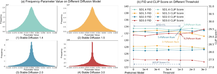
Figure 2: (a) Weight distributions of the pre-trained parameters in Stable Diffusion (SD) 1.4, 1.5, 2.0, and 3.0, which all belong to a Gaussian distribution, therefore a large number of parameters are around $0$. (b) The performance (FID on the left axis and CLIP Score on the right) of SD Models when the parameters in the pre-trained models with absolute values smaller than a certain threshold are set to $0$.

3.1 Ineffective parameters in Stable Diffusion models

Based on the theorem of model pruning proposed in (Liang et al., 2021), which regards the parameters with the smallest absolute values as “ineffective” parameters, we investigated the effectiveness of these parameters in diffusion models. In order to draw general and reliable conclusions, we conducted studies on Stable Diffusion versions 1.4, 1.5, 2.0, and 3.0. We set parameters with absolute values below a certain threshold $\theta_{t}$ (from $10^{-3}$ to $10^{-5}$) to zero, and evaluated the performance of the regularized models on generative tasks. Following the evaluation metrics of Stable Diffusion 3.0 (Esser et al., 2024), we use CLIP Score (Radford et al., 2021) and Fréchet Inception Distance (FID) (Heusel et al., 2017) to measure the generation ability of different versions of the Stable Diffusion (SD) model.

The results are shown in Fig. 2(b). We observed that within a certain threshold range $\theta_{t}\in(0,10^{-3}]$, with the small parameters set to $0$, the generative ability of the SD models is minimally affected. And in some cases, the regularized model with “ineffective” parameters set to $0$ even outperforms the original model (i.e., no parameters are set to $0$, with $\theta_{t}=0$). Specifically, SD1.4 and SD1.5 show better FID scores than the original model when thresholds are in the range of $\theta_{t}\in[5\times 10^{-4},10^{-3}]$, and SD2.0 and SD3.0 exhibit superior FID scores at a threshold of $\theta_{t}=10^{-4}$. These results show that parameters with the smallest absolute values have a limited impact on the generative process, and in some cases, they may even slightly impair the model’s generative ability.

3.2 Unstable Training Process Contributes to Useless Parameters

Sec. 3.1 demonstrated that parameters with smaller absolute values have minimal impact on the generative capability of diffusion models. A natural question arises: are these currently ineffective parameters caused by the model structure and inherently redundant, or are they caused by the training process and can become effective again? If it is the former case, the structural design of the model prevents these parameters from learning effective information, then these parameters are redundant and unlikely to be useful in subsequent training processes. While if it is the latter case, these parameters are potentially effective when leveraged rationally in the subsequent training. Therefore, we further investigated the reasons behind the ineffectiveness of these parameters, and found that the ineffectiveness is due to the randomness of the optimization process, rather than an inherent inability caused by model structure.

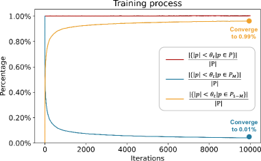
Figure 3: The changes of parameters whose absolute values are bewlow the $1\%$ theshold $\theta_{t}$ during full-parameter fine-tuning. The parameters originated from both the initially below-threshold $P_{M}$ and the initially above-threshold $P_{1-M}$, with the blue and yellow curves showing the proportions of these two groups. The blue curve shows that the proportion of $P_{M}$ remaining below $\theta_{t}$ gradually decreased from $100\%$ to $1\%$. While the yellow curve shows $1\%$ ($0.99\%$ out of $99\%$) of the initially above-threshold $P_{1-M}$ eventually fell below $\theta_{t}$. The results validate that the ineffective parameters arise from the randomness of the network optimization process, rather than inherently redundant. With the help of our model, more than 99.95% parameters can be effectively used, which can mitigate this problem.

Specifically, we employed a Stable Diffusion model pre-trained on the FFHQ dataset (Karras et al., 2019), whose parameter matrices are denoted as $P_{0}$. We recorded the parameters in the pre-trained model with absolute values below the $1\%$ threshold $\theta_{t}$ by a parameter mask $M$, where $P_{M}=P_{0}\odot M$ denotes the initially below-threshold parameters ($1\%$ of all parameters), and $P_{1-M}=P_{0}\odot(1-M)$ denotes the initially above-threshold parameters ($99\%$ of all parameters), satisfying:

$$\left|p\right|<\theta_{t}, \forall p\in P_{M},$$ (1)

$$\left|p\right|\geq\theta_{t}, \forall p\in P_{1-M}.$$

Then, we continue training this pre-trained model on the FFHQ dataset, and observe the changes of its parameters $P$ during the training process. During this fine-tuning stage, we recorded the “source” of parameters whose absolute values are below the threshold $\theta_{t}$ ($\{\left|p\right|<\theta_{t}\}$), i.e., whether they are initially below-threshold or initially above-threshold. And we found that these parameters originated from both the initially below-threshold $P_{M}$ and the initially above-threshold $P_{1-M}$.

The proportions of these two groups and how they change during the finetuning are shown in Fig. 3. As the training progressed, the proportion of $P_{M}$ remaining below $\theta_{t}$ gradually decreased from $100\%$ to $1\%$ (blue curve decreases from $1.00\%$ to $0.01\%$); while $1\%$ of the initially above-threshold $P_{1-M}$ eventually fell below $\theta_{t}$ (yellow curve raises from $0.00\%$ to $0.99\%$). The results indicate that initially ineffective parameters $P_{M}$ caused by the randomness of the training process, mostly become effective over time (only $1\%$ remaining below threshold). Conversely, some initially effective parameters become ineffective as training continues.

This pheonomenon demonstrates that the ineffectiveness of parameters is not inherent to model structure, but rather a result of the stochastic nature of the training process, which causes some parameters to fall below the threshold $\theta_{t}$ at the last training step coincidentally, making them temporarily ineffective. As the training continues, most of these parameters regain effectiveness, proving their potentially effectiveness, which motivates us to leverage these temporarily ineffective parameters to fine-tune the pre-trained model.

Algorithm 1 SaRA Fine-tuning Pseudocode

1:model = Initialize_model()

2:# optimizer = AdamW(model.parameters())

3:optimizer = AdamW-SaRA(model, threshold = $\theta_{t}$)

4:for epoch = 1 to $N$ do

5:     for each mini-batch $(x,y)$ do

6:         $y_{\text{pred}}=\text{model}(x;\theta)$

7:         $loss=\text{Loss\_Func}(y_{\text{pred}},y)$

8:         $loss.\text{backward}()$

9:         optimizer.step()

10:     end for

11:end for

4 Progressive sparse low-rank model adaptation

Inspired by the potential effectiveness of parameters with the smallest absolute values, as discussed in Sec. 3, we propose SaRA, a novel parameter-efficient fine-tuning method designed to fully utilize these temporarily ineffective parameters. Specifically, we first identify the ineffective parameters in the pre-trained parameters $P_{0}$ by computing a sparse mask $M=P_{0}<\theta_{t}$, where $\theta_{t}$ is a threshold and the sparse mask only selects a small portion from all parameters. We then use this sparse mask to update the initially ineffective parameters $P\odot M$, while keeping the initially effective parameters $P\odot(1-M)$ frozen. This approach enables the pre-trained model to acquire new capabilities for downstream tasks (through the learnable $P\odot M$) while preserving prior information (through the fixed $P\odot(1-M)$). To avoid the problem of overfitting caused by strong representation ability due to the potential high rank of the learnable sparse matrix $P\odot M$, we propose a nuclear norm-based low-rank loss to mitigate overfitting (Sec. 4.2). In addition, we propose a progressive parameter adjustment strategy to further make full use of the ineffective parameters by progressively reselecting them (Sec. 4.3). Finally, we propose an unstructured backpropagation strategy, which significantly reduces memory costs and can be applied to enhance all selective PEFT methods. Our SaRA method is efficiently encapsulated and can be implemented by modifying just one line of code compared to the training script, which is shown in Alg. 1.

4.1 Fine-tuning on the potential effective parameters

In Sec. 3, we have demonstrated that parameters with smaller absolute values are ineffective in the generative process of diffusion models, and this ineffectiveness is not due to the model’s architecture but rather the stochastic nature of the optimization process. Therefore, we propose SaRA, which fine-tunes these temporarily ineffective parameters to adapt the pre-trained diffusion model to downstream tasks, enabling it to learn new knowledge while preserving its original generative capability as much as possible. Specifically, we first obtain a mask $M$ for the initial parameter set $P_{0}$, which satisfies:

$$\left|p\right|<\theta_{t},\forall p\in P_{0}\odot M,$$ (2)

where $M$ is a sparse matrix, since the theshold $\theta_{t}$ is set low and only selects a small portion from all the parameters. We then use this sparse mask to update the initially ineffective parameters $P\odot M$, while keeping the initially effective parameters $P\odot(1-M)$ frozen. During training, for the gradient $\nabla P$ of the parameters, we use the pre-defined sparse mask $M$ to retain the gradients we need and update the corresponding parameters $P_{M}{\color[rgb]{0,0,0}=P\odot M}$ by:

$$\nabla P_{M} =\nabla P\odot M+\mathbf{0}\odot(1-M),$$ (3)

$$P_{new} =P-\lambda\cdot\nabla P_{M}.$$

In this way, we can focus on training the ineffective parameters while keeping the other parameters unchanged, ensuring the original generation ability of the pre-trained model is preserved, while learning new knowledge by the parameters $P_{M}$.

4.2 Nuclear Norm-based Low-Rank Constraint

The sparse parameter matrices $P_{M}$ can sometimes have a high rank, resulting in strong representational capabilities that may lead to overfitting during the training process of downstream tasks. To mitigate this issue, we introduce a nuclear norm-based low-rank constraint on the sparse matrix to prevent the rank from becoming excessively high during the training process.

A direct way to apply low-rank constraint is to minimize the rank of the sparse parameter matrix $Rank(P)$ as a constraint. However, directly minimizing the rank function is computationally intractable due to its non-convex nature. Therefore, we use the nuclear norm of the matrix to estimate its rank:

$$\|P\|_{*}=\sum_{i}\sigma_{i}(P),$$ (4)

where $\sigma_{i}$ are the singular values of $P$. By minimizing the nuclear norm, we can constrain the rank of the sparse matrix in a computationally efficient way.

To compute the nuclear norm $\|P\|_{*}$, we employ the singular value decomposition (SVD) of the matrix $P=U\Sigma V^{T}$, where $U$ and $V$ are orthogonal matrices, and $\Sigma$ is a diagonal matrix containing the singular values $\sigma_{i}(P)$. The subgradient of the nuclear norm at $P$ has been derived by (Watson, 1992), which can be expressed as:

$$\partial\|P\|_{*}=\{UV^{T}+W\mid W\in R^{m\times n},\,U^{T}W=0,\,WV=0,\,\|W\|_{2}\leq 1\}.$$ (5)

Based on this derivation of the nuclear norm gradient, we can ensure that gradient descent methods can be employed to incorporate nuclear norm-based low-rank constraints into the training process, thereby achieving our nuclear norm-based low-rank constrained loss:

$$L_{rank}=\|P\|_{*}=\sum_{i}\sigma_{i}(P).$$ (6)

4.3 Progressive parameter adjustment

As discussed in Sec. 3.2 and Fig. 3, when continuing training the pre-trained model, the initially ineffective parameters gradually become above threshold and effective, with only $1\%$ of initially ineffective parameters remaining below threshold eventually. However, the speed at which ineffective parameters become effective (the slope of blue curve in Fig. 3) varies during the finetuning process. In the early stage of the finetuning process (e.g., the first $2.5$k iterations), a large portion (over $80\%$) of initially ineffective parameters quickly become effective, with a small part (less than $20\%$) remaining below threshold. However, the speed slows down in the later stage of finetuning: from $2.5$k to $8$k iterations, the small portion of remaining below-threshold parameters jumps out of the theshold very slowly. However, the finetuning iterations are typically limited (e.g., a few thousands), in which case the slow speed in the later finetuning stage can cause problems: the remaining below-threshold ineffective parameters may not be trained to be effective and fully utilized.

To address this issue, we propose a progressive parameter adjustment strategy. To alleviate the slow speed of ineffective parameters becoming effective in the later stage, this strategy reselects the ineffective parameters that remain below threshold (about $15\%$-$20\%$ of initial ineffective parameters) after the early finetuning stage, and focuses on optimizing these remaining below-threshold parameters in the subsequent finetuning stage. Compared to the finetuning without this reselecting operation, this strategy can quickly make remaining ineffective parameters effective again in the later finetuning stage.

Specifically, we introduce a parameter readjustment phase. After the early finetuning stage (we set the first half of the total iterations as the early finetuning stage, e.g., 2,500 iterations when there are 5,000 finetuning iterations) on the initially selected below-threshold parameters $P^{0}_{learn}$, we reselect parameters from $P^{0}_{learn}$ that remain below the predefined threshold as new trainable parameters $P_{M}$ (which is a subset of $P^{0}_{M}$ and typically has $15\%$-$20\%$ of $P^{0}_{M}$’s parameters). Then in the subsequent finetuning stage, we only optimize this subset of initial ineffective parameters, and keep other parameters of $P^{0}_{learn}$ frozen. By focusing on optimizing the small subset of remaining below-theshold parameters, this strategy greatly improves the speed of ineffective parameters jumping out of the theshold in the later finetuning stage, thereby enhancing the model’s adaptation capability. In our experiments, we found that under the same number of finetuning iterations, models without the progressive parameter adjustment strategy had $15\%$ of $P^{0}_{learn}$ parameters that remained ineffective after the finetuning, while models with the progressive strategy only had $2\%$ of $P^{0}_{learn}$ parameters that were still ineffective. The results indicate this strategy significantly improves the performance of our method during the fine-tuning process.

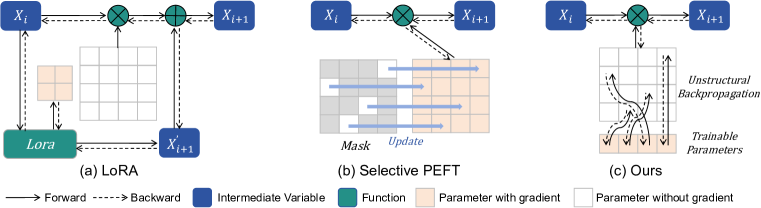
Figure 4: Visualization of our unstructural backpropagation. From left to right: the computation graph in the training process for LoRA (Hu et al., 2021), Selective PEFT method (Ansell et al., 2021; Guo et al., 2020), and our unstructural backpropagation method. a) LoRA stores an additional intermediate variable $X^{\prime}_{i+1}$ in each LoRA layer, and b) selective PEFT methods store the gradients for the whole parameters matrices, along with a parameter mask in each layer, causing a waste of memory and computation resources. c) In contrast, our Unstructural Backpropagation method extracts the trainable parameters, sets them as independent leaf nodes, and only retains gradients for them. Our strategy enables the gradients to flow from the whole parameter matrices to the sparse parameters to be trained, largely improving the memory efficiency during the training process.

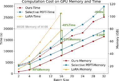
Figure 5: The computation cost on GPU memory and Time of different methods (LoRA, Selective PEFT method (LT-SFT) and Ours) when training the Stable Diffusion 2.0 on different batch sizes. It can be seen that our method saves a large amount of GPU memory and computation time compared to LoRA and Selective PEFT method.

4.4 Unstructural Backpropagation

Currently, both the LoRA-based methods (the same for the adapter-based methods) and selective PEFT methods cause a heavy burden on the computation resources: 1) For the LoRA-based methods, since the LoRA module is additional to the original model, there is no need to store the gradients of the model parameters, but they still require additional memory costs to store the intermediate variables in the LoRA module, which is shown in Fig. 4 (a). 2) And for the selective PEFT methods, a persistent issue is that they require the same or even more computational resources (especially GPU memory) as full-parameter fine-tuning. Although they only finetune a subset of the model’s parameters for fine-tuning, they retain the gradients of the entire parameter matrices $P$, because the mainstream deep learning libraries (such as PyTorch and TensorFlow) only support gradient backpropagation and updates for the entire parameter matrices. Consequently, previous selective PEFT methods had to perform gradient backpropagation on the entire parameter matrices $P$, and then use pre-computed mask matrices $M$ to mask out the gradients of unnecessary parameters by $\nabla P_{M}=M\odot\nabla P$, and perform an overall parameter update by $P_{new}=P-\lambda\nabla P_{M}$ (visualized in Fig. 4 (b)). This approach necessitates storing the gradients of all model parameters and the additional mask matrices, leading to greater computational resource demands than full-parameter fine-tuning. This clearly contradicts the “efficient” requirements of PEFT and limits the practical applications of such methods.

To address this issue, we propose Unstructural Backpropagation (shown in Fig. 4 (c)), which supports efficient gradient backpropagation and updates for unstructured parameters. Different from previous selective PEFT methods that require retaining the gradient for the whole parameter matrices, our Unstructural Backpropagation only needs to retain gradients for the selected subset of below-threshold parameters $P_{M}$. Specifically, we first store the mask matrices $M$ corresponding to each layer’s parameters that need to be trained. In the computational graph, we deviate from the traditional approach of setting model parameters as leaf nodes. Instead, we extract the trainable parameters $P_{learn}=P[M]\in\mathcal{R}^{\|M\|_{0}}$ and set them as independent leaf nodes, where $[\cdot]$ denotes element-wise indexing of the matrix. I.e., as shown in Fig. 4 (c), we extract the subset of trainable parameters and combine them into a separate parameter vector, and only retain gradients for this vector. Then, during the forward pass, we define an Unstructural Mapping function $UM(\cdot)$ to update the model parameters $P$ by:

$$P=UM(P,P_{learn},M),{\color[rgb]{0,0,0}where}\begin{cases}P[M]&=P_{learn},\\ P[1-M]&=P[1-M].\end{cases}$$ (7)

And the updated model paramaters $P$ will then participate in the training process. During backpropagation, we define the Unstructural Backpropagation function $UB(\cdot)$ to propagate the gradients from the model parameters to the trainable parameters by:

$$\nabla P_{learn}=UB(\nabla P,M)=\nabla P[M].$$ (8)

In this way, during the backpropagation process, the gradients on the model parameters $\nabla P$ will be automatically cleared, since it is no longer a leaf node, and only the gradients on the learnable parameters $\nabla P_{learn}$ are stored, which significantly reduces the GPU memory usage during the fine-tuning process.

5 Experiments

5.1 Experiment Settings

Experimental Tasks and Baselines. To validate the effectiveness of our method in generative tasks, we first conduct experiments on various tasks, including backbone fine-tuning, downstream dataset fine-tuning, image customization, and controllable video generation. We compare our method with three state-of-the-art parameter efficient fine-tunining methods: LoRA (Hu et al., 2021), Adaptformer (Chen et al., 2022), and LT-SFT (Ansell et al., 2021); along with the full-parameter fine-tuning method.

Metrics. We evaluate the generation models by three metrics: 1) Fréchet Inception Distance (FID) (Heusel et al., 2017) to measure the similarity between the generated image distribution and target image distribution, where a lower score indicates better similarity; 2) CLIP Score to measure the matching degree between the given prompts and generated images with a CLIP L/14 backbone (Radford et al., 2021), where a higher score indicates better consistency; 3) Additionally, since FID and CLIP scores exhibit a certain degree of mutual exclusivity in finetuning a text-to-image model to downstream tasks (i.e., an overfitted model will result in the best FID but the worst CLIP score), we introduce a new metric, the Visual-Linguistic Harmony Index (VLHI), which is calculated by adding the normalized FID and CLIP scores, to balance the evaluation of style (FID) and the preservation of model priors (CLIP score), where a higher score indicates better performance. The detailed definition and calculation process of VLHI can be found in the Appendix.

5.2 Backbone Fine-tuning

Backbone Fine-tuning. Different from the previous parameter-efficient fine-tuning methods that mainly aim to fine-tune the pre-trained model to downstream tasks, our model enables the pre-trained model to make full use of the parameters. In other words, our finetuning method can improve the performance of pre-trained models on the main task (the original task it is trained on), by optimizing the initially ineffective parameters to be effective and thus increasing the number of effective parameters. Therefore, apart from experimenting on downstream tasks like traditional PEFT methods, we first apply our method to the main task of the pre-trained model, continuing to fine-tune the backbone on the original training dataset, in order to explore whether our method can enhance the base model’s performance. Specifically, we employ the pre-trained Stable Diffusion models on ImageNet (Deng et al., 2009), FFHQ (Karras et al., 2019), and CelebA-HQ (Karras et al., 2017) datasets, and fine-tune them on these pre-trained datasets for 10K iterations. We compare our method with full-parameter finetuning, LoRA, AdaptFormer, and LT-SFT by computing the FID metric between 5K generated data and 5K randomly sampled data from the source dataset. The results are shown in Fig. 6, which demonstrates that our method achieves the best FID scores, indicating our method effectively improves the performance of the pre-trained models on the main task.

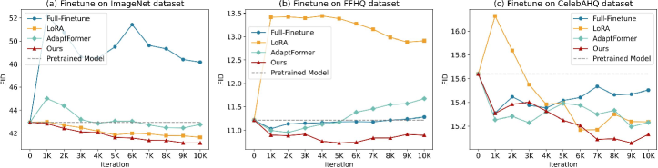
Figure 6: Quantitative comparison among different PEFT methods on Backbone Fine-tuning on ImageNet, FFHQ, and CelebA-HQ datasets. Our method achieves the best FID scores, indicating our method effectively improves the performance of the pre-trained models on the main task.

5.3 Model Fine-tuning on Downstream Datasets

Downstream Dataset Fine-tuning. In this experiment, we choose 5 widely-used datasets from CIVITAI with 5 different styles to conduct the fine-tuning experiments, which are Barbie Style, Cyberpunk Style, Elementfire Style, Expedition Style and Hornify Style. Each dataset contains about $200\sim 400$ images, and for each image, we employ BLIP model (Li et al., 2022) to generate its text annotations. We compare our model with LoRA (Hu et al., 2021), Adaptformer (Chen et al., 2022), LT-SFT (Ansell et al., 2021) and full-parameter finetuning method. To comprehensively compare PEFT methods, we conduct three sets of experiments for each PEFT method on Stable Diffusion 1.5, 2.0, and 3.0, with selected trainable parameter sizes of 50M, 20M, and 5M. This allows us to explore the performance of different methods under varying trainable parameter sizes. We train all methods for 5,000 iterations and use the trained models to generate 500 images based on 500 text descriptions (generated by GPT-4). Part of the qualitative comparison results (Stale Diffusion 1.5, 50M parameters) are shown in Fig. 7 (For more results, please refer to the appendix). It can be seen that our model can learn the style accurately while generating images that are well consistent with the given text prompts under different datasets.

We then calculate the FID score between the generated images and the dataset, and the CLIP score between the generated images and the text descriptions, along with the VLHI, which measures both the style (FID) and generalization (CLIP score). The quantitative results are shown in Tab. 1, from which we can draw the following conclusions: 1) Our model can always achieve the best VLHI on average across five datasets, indicating that our model can preserve the prior information in the pre-trained model well (a good CLIP score), while learning as much task-specific knowledge as possible (a good FID), outperforming all the other PEFT methods and full-finetune method; 2) As the number of learnable parameter increases, our model can learn more task-specific knowledge (better FID), but may lose part of the prior information (lower CLIP score); 3) For Stable Diffusions 1.5 and 2.0, our model achieves the best FID and usually the sub-optimal CLIP score on average across five datasets, and under different parameter numbers; while for Stable Diffusion 3.0, which has much more parameters than SD 1.5 and 2.0, our model achieves the best CLIP score and usually the suboptimal FID on average across five datasets. The results indicate that for a larger pre-trained model, more learnable parameters are needed to learn the task-specific knowledge well.

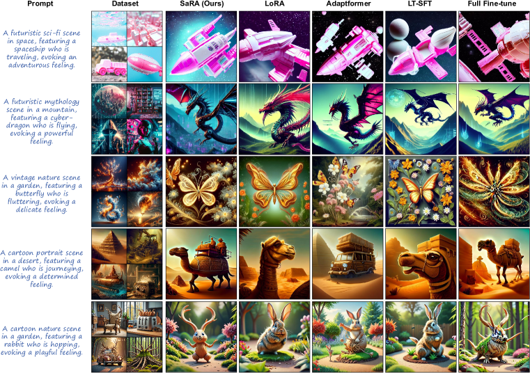
Figure 7: The comparison among different kinds of PEFT methods on fine-tuning to the target domain, which are Barbie style, Cyberpunk style, Elementfire style, Expedition style, and Hornify style from top to bottom. Our methods can learn the target domain style accurately while achieving good alignment between the generated images and the text prompts.

Backbone	Model	Params	BarbieCore			Cyberpunk			ElementFire			Expedition			Hornify			Mean
			FID $\downarrow$	CLIP $\uparrow$	VLHI $\uparrow$	FID $\downarrow$	CLIP $\uparrow$	VLHI $\uparrow$	FID $\downarrow$	CLIP $\uparrow$	VLHI $\uparrow$	FID $\downarrow$	CLIP $\uparrow$	VLHI $\uparrow$	FID $\downarrow$	CLIP $\uparrow$	VLHI $\uparrow$	FID $\downarrow$	CLIP $\uparrow$	VLHI $\uparrow$
SD 1.5	50M	LoRA	161.88	29.93	1.34	117.49	28.22	1.85	181.66	27.47	1.20	136.31	27.39	1.32	156.36	26.80	1.28	150.74	27.96	1.45
		Adaptformer	166.09	29.00	1.00	126.21	27.13	0.66	151.27	26.57	1.29	138.01	26.41	0.63	151.53	26.20	1.18	146.62	27.06	1.18
		LT-SFT	157.80	23.80	0.54	123.59	25.71	0.45	171.67	25.11	0.44	139.29	27.81	1.46	158.52	26.35	1.06	150.18	25.76	0.49
		SaRA (Ours)	148.54	28.60	1.75	121.67	27.30	1.15	132.67	26.77	1.63	131.56	27.34	1.48	140.36	25.40	1.15	134.96	27.08	1.55
	20M	LoRA	159.64	29.65	1.40	117.21	28.43	1.95	174.79	27.61	1.35	136.38	27.00	1.07	155.85	27.16	1.43	148.77	27.97	1.52
		Adaptformer	159.02	29.08	1.34	123.88	28.07	1.19	174.17	26.53	0.95	137.03	26.67	0.83	157.09	26.63	1.20	150.24	27.39	1.21
		LT-SFT	156.60	23.76	0.59	119.75	25.33	0.70	191.01	25.96	0.49	144.57	28.01	1.37	165.47	26.89	1.10	155.48	25.99	0.42
		SaRA (Ours)	153.68	29.33	1.63	116.69	28.24	1.94	138.64	26.63	1.50	129.98	27.04	1.36	145.62	26.40	1.39	136.92	27.53	1.69
	5M	LoRA	163.80	29.93	1.25	117.58	28.32	1.88	184.99	27.74	1.25	137.96	27.10	1.07	153.57	26.93	1.40	151.58	28.00	1.44
		Adaptformer	164.22	29.37	1.14	120.98	28.11	1.48	184.84	26.66	0.84	143.01	27.35	1.01	171.34	26.85	0.94	156.88	27.67	1.13
		LT-SFT	169.24	24.23	0.08	127.01	25.43	0.03	202.47	26.90	0.68	153.49	27.96	0.97	176.41	27.34	1.00	165.72	26.37	0.27
		SaRA (Ours)	153.69	29.39	1.64	118.74	28.17	1.72	174.86	27.04	1.13	134.45	27.06	1.18	157.24	26.97	1.33	147.80	27.73	1.44
	860M	Full-finetune	147.81	27.77	1.65	120.22	27.84	1.47	136.49	25.10	0.95	129.07	26.75	1.21	134.86	24.64	1.00	133.69	26.42	1.30
SD 2.0	50M	LoRA	157.41	29.81	1.64	133.22	28.00	1.52	187.32	27.70	1.29	148.18	27.58	1.38	169.92	26.99	1.09	159.21	28.02	1.51
		Adaptformer	161.87	30.78	1.75	138.02	27.85	1.12	179.44	27.35	1.26	162.45	27.06	0.47	175.39	26.59	0.76	163.43	27.93	1.25
		LT-SFT	164.80	28.13	0.59	134.97	26.40	0.59	183.23	25.90	0.50	153.94	27.88	1.33	167.19	26.83	1.08	160.83	27.03	0.57
		SaRA (Ours)	162.72	29.72	1.31	135.05	28.30	1.55	151.82	27.24	1.68	138.77	26.30	0.96	165.62	26.71	1.05	150.80	27.65	1.55
	20M	LoRA	161.92	30.18	1.52	129.01	28.36	2.00	190.90	27.72	1.24	147.05	27.60	1.44	168.03	26.97	1.13	159.38	28.16	1.63
		Adaptformer	160.29	30.42	1.70	141.80	27.92	0.89	190.57	27.33	1.05	157.31	27.07	0.69	175.39	26.59	0.76	165.07	27.86	1.13
		LT-SFT	168.09	28.29	0.47	135.03	26.47	0.62	194.17	26.64	0.66	155.51	27.88	1.27	174.64	27.12	1.04	165.48	27.28	0.59
		SaRA (Ours)	164.57	30.22	1.39	134.28	28.29	1.60	163.67	27.90	1.79	149.29	27.01	0.98	165.62	26.71	1.05	155.49	28.03	1.68
	5M	LoRA	162.47	29.91	1.39	132.35	28.13	1.65	183.55	27.68	1.34	152.69	27.41	1.09	164.00	26.81	1.15	159.01	27.99	1.49
		Adaptformer	162.25	30.52	1.63	143.41	27.69	0.66	188.42	27.45	1.15	160.23	27.37	0.76	180.07	26.72	0.71	166.88	27.95	1.12
		LT-SFT	175.45	28.74	0.23	137.84	26.55	0.46	209.51	27.29	0.70	161.67	27.90	1.03	186.69	27.62	1.00	174.23	27.62	0.52
		SaRA (Ours)	165.57	30.58	1.47	136.89	27.77	1.15	174.73	27.60	1.45	150.89	27.29	1.09	166.40	26.90	1.13	158.90	28.03	1.53
	866M	Full-finetune	160.87	29.30	1.25	133.19	28.33	1.70	198.45	25.81	0.19	137.84	26.74	1.27	145.99	25.64	1.00	155.27	27.16	0.93
SD 3.0	50M	LoRA	165.22	29.57	1.28	123.59	28.38	1.59	187.26	27.54	1.36	148.38	26.83	1.50	169.00	26.96	1.35	158.69	27.85	1.52
		Adaptformer	164.09	29.81	1.43	126.73	28.23	1.38	186.05	27.14	0.93	156.77	27.12	1.62	180.11	26.91	1.09	162.75	27.84	1.41
		LT-SFT	209.04	29.45	0.39	158.59	27.72	0.10	208.94	27.03	0.14	204.16	26.02	0.00	189.26	26.06	0.38	194.00	27.26	0.18
		SaRA (Ours)	170.73	30.63	1.73	128.35	28.45	1.50	179.87	27.63	1.68	137.92	26.47	1.35	158.86	27.10	1.65	155.15	28.06	1.77
	20M	LoRA	156.23	30.18	1.77	123.12	28.22	1.48	187.14	27.76	1.62	143.59	26.96	1.68	174.62	26.63	1.03	156.94	27.95	1.64
		Adaptformer	174.32	30.30	1.49	128.73	28.31	1.39	175.60	27.77	1.96	150.69	26.50	1.19	174.61	26.56	0.99	160.79	27.89	1.50
		LT-SFT	167.02	29.19	1.05	154.04	27.67	0.19	203.23	26.91	0.16	155.68	26.48	1.10	177.42	26.21	0.71	171.48	27.29	0.77
		SaRA (Ours)	166.21	30.41	1.70	126.69	28.19	1.35	180.74	27.31	1.28	150.15	26.88	1.52	163.78	27.01	1.48	157.52	27.96	1.64
	5M	LoRA	161.80	30.14	1.64	124.17	28.06	1.33	174.66	27.27	1.40	149.85	27.01	1.63	172.56	26.88	1.23	156.61	27.87	1.59
		Adaptformer	168.98	30.50	1.69	127.35	27.89	1.11	204.69	27.71	1.05	158.60	27.03	1.52	182.22	26.88	1.03	168.37	28.00	1.40
		LT-SFT	158.26	29.29	1.27	134.81	27.69	0.75	181.68	27.27	1.20	153.52	27.20	1.74	193.25	26.61	0.63	164.30	27.61	1.20
		SaRA (Ours)	174.42	30.60	1.64	125.14	28.91	1.94	194.79	27.63	1.24	157.20	27.17	1.65	181.39	27.20	1.24	166.59	28.30	1.68
	2085M	Full-finetune	162.33	28.69	0.88	151.57	27.59	0.20	174.12	27.16	1.29	135.28	26.09	1.06	144.56	25.58	1.00	153.57	27.02	1.00

Table 1: Comparison with different parameter-efficient fine-tuning methods (LoRA Hu et al. (2021), Adaptformer Chen et al. (2022), and LT-SFT Ansell et al. (2021)), along with full-parameter fine-tuning on Stable Diffusion 1.5, 2.0, and 3.0. For most of the conditions, our model achieves the best FID and VLHI score, indicating that our model learns domain-specific knowledge successfully while keeping the prior information well. Bold and underline represent optimal and sub-optimal results, respectively.

5.4 Omni-Application Across Diverse Sphere Tasks

Image Customization. Image customization aims to learn a common subject from a few images and then apply it to new images. Dreambooth (Van Le et al., 2023) is a representative method for image customization, which trains the UNet of a diffusion model to bind the target subject to a rare token (e.g., ‘sks’), and then generates images with the specified content based on the rare token. Since Dreambooth requires fine-tuning the UNet network, we compare the performance of full-finetune (original Dreambooth), LoRA, Adaptformer, LT-SDT, and our method in image customization. As shown in Fig. 8, our method can learn the subject content while preserving the prior information of the diffusion model, thereby improving the consistency between the generated images and the given texts. We further calculate the CLIP Score (Radford et al., 2021) between the generated images and the given text (denoted as CLIP-Text), and the CLIP Score between the generated images and the source images (CLIP-IMG), along with VLHI balancing both the two metrics. As shown in Tab. 2, LoRA achieves a high CLIP-IMG score but the lowest CLIP-Text score, indicating a severe overfitting problem. This problem is also evident in Figure 8, where the generated cases do not align with the texts. Other PEFT methods, including full-parameter fine-tuning, achieve relatively low CLIP-IMG and CLIP-Text scores. In contrast, our method achieves the best CLIP-Text score, a competitive CLIP-IMG score (only lower than the overfitted LoRA), and the best average VLHI score across three datasets, demonstrating its effectiveness in image customization task.

Figure 8: Qualitative comparisons among different PEFT methods on image customization by fine-tuning the UNet model in Dreambooth (Van Le et al., 2023). Our model can accurately capture the target feature while preventing the model from overfitting, outperforming Dreambooth with other PEFT methods and Textual inversion (Gal et al., 2022).

0000000Methods	Dog			Clock			Backpack			Mean
	CLIP-I $\uparrow$	CLIP-T$\uparrow$	VLHI $\uparrow$	CLIP-I $\uparrow$	CLIP-T $\uparrow$	VLHI $\uparrow$	CLIP-I $\uparrow$	CLIP-T $\uparrow$	VLHI $\uparrow$	CLIP-I $\uparrow$	CLIP-T $\uparrow$	VLHI $\uparrow$
Textual Inversion	0.788	23.94	0.36	0.789	24.15	1.00	0.654	24.09	0.00	0.744	24.06	0.39
Dreambooth + Full Fine-tune	0.776	25.85	1.13	0.894	22.39	1.13	0.856	25.44	1.76	0.842	24.56	1.36
Dreambooth + LoRA	0.895	23.64	1.00	0.913	21.71	1.00	0.917	25.23	1.84	0.908	23.53	1.00
Dreambooth + Adaptformer	0.772	25.42	0.91	0.885	23.18	1.38	0.873	25.25	1.69	0.843	24.62	1.41
Dreambooth + LT-DFT	0.757	23.94	0.13	0.893	22.45	1.14	0.869	25.00	1.49	0.840	23.80	0.79
Dreambooth + SaRA (Ours)	0.790	25.87	1.24	0.887	23.51	1.53	0.886	25.27	1.76	0.854	24.88	1.67

Table 2: Quantitative comparisons between different PEFT methods on image customization by fine-tuning the UNet model in Dreambooth.

Controllable Video Generation. We further investigate the effectiveness of our method in fine-tuning video generation models. AnimateDiff (Guo et al., 2023) is a representative video generation model based on Stable Diffusion (Rombach et al., 2022), which inserts temporal attention modules between the original spatial attention modules to model temporal correlations, enabling a diverse text-to-video generation. To achieve more controllable generation, AnimateDiff fine-tunes the temporal attention module using different camera motion data, such as Pan Left, Pan Right, Zoom In, and Zoom Out, to control the camera movements precisely. We compare the effectiveness of various PEFT methods in fine-tuning AnimateDiff for three types of camera movements, including Zoom In, Zoom Out, and Pan Right. Specifically, we collected 1,000 video-text pairs with identical camera movements for each type of camera motion. The temporal attention modules are fine-tuned using full fine-tuning, LoRA, Adaptformer, LT-SDT, and our SaRA. As shown in Fig. 9, the compared methods usually suffer from generating artifacts in the results (shown in red boxes), indicating that these methods have lost some model priors of specific content during the fine-tuning process. Moreover, for the sea turtle examples, full fine-tuning, LoRA, and LT-SFT exhibit noticeable content degradation. And for the pan-right examples, all the compared methods fail to capture the photographer, indicating a significant model overfitting problem. In contrast, our method achieves excellent camera motion control while achieving good consistency between the video content and the text.

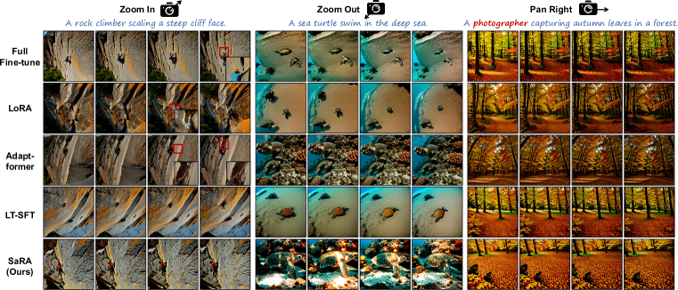
Figure 9: The comparison results of the video generation model (Guo et al., 2023), fine-tuned using different PEFT methods on three video datasets featuring zoom-in, zoom-out, and pan-right camera motions. The red boxes highlight artifacts generated by the compared methods, indicating that these methods have lost some model priors of specific content during the fine-tuning process. In the sea turtle examples, full fine-tuning, LoRA, and LT-SFT exhibit noticeable content degradation. And for the pan-right examples, all the compared methods fail to capture the photographer, indicating significant model overfitting. In contrast, our method achieves excellent camera motion control while preserving video content well.

00000000Method	FID $\downarrow$	CLIP Score $\uparrow$	VLHI $\uparrow$
w/o. $PPA$ &$\mathcal{L}_{rank}$	134.75	27.01	1.16
w. $PPA$, w/o. $\mathcal{L}_{rank}$	130.95	26.66	1.56
w. $\mathcal{L}_{rank}$, w/o. $PPA$	135.31	27.12	0.89
w. $PPA$ &$\mathcal{L}_{rank}$ (Ours)	131.56	27.34	1.79
Tuning Largest Parameters	130.55	25.42	1.00
Tuning Random Parameters	133.57	26.58	0.97

Table 3: Quantitative ablation studies on six ablated models: 1) model without PPA and $\mathcal{L}_{rank}$, 2) model with PPA, but without $\mathcal{L}_{rank}$, 3) model with $\mathcal{L}_{rank}$, but without PPA, 4) model with both PPA and $\mathcal{L}_{rank}$ (ours), 5) model fine-tuned with the largest absolute values parameters, and 6) model fine-tuned with randomly selected parameters. The full version of our model achieves the best VLHI, CLIP Score, and good FID.

5.5 Analysis on Training efficiency

In Sec. 4.4, we propose unstructural backpropagation, which allows selective PEFT to store and update only the gradients of trainable parameters, significantly reducing memory usage during training. We conducted experiments on the Stable Diffusion 2.0 model using an 80G NVIDIA A100 GPU, comparing the memory usage and training time of LT-SFT (Selective PEFT method), LoRA, and our method across different batch sizes. The results, shown in Fig. 5, demonstrate that our method achieves the lowest memory consumption and training time under all batch sizes. Compared to LT-SFT, we reduce memory usage by a fixed 9.2G (equivalent to the total gradient size of fixed parameters) and achieve over 45% memory reduction for smaller batch sizes. Furthermore, compared to LoRA, our method saves over 52% memory and 49% training time for larger batch sizes, showcasing the efficiency of our SaRA in model fine-tuning.

5.6 Ablation Studies

In this section, we first conduct ablation studies to validate the effectiveness of our proposed modules: 1) the progressive parameter adjustment (PPA), and 2) the low-rank constrained loss ($\mathcal{L}_{rank}$). Then, we further assess the effectiveness of training parameters with the smallest absolute values, by comparing different parameter-selection strategies, including selecting the largest parameters and random parameters. We conduct downstream dataset finetuning experiments using the Expedition dataset comparing six ablated models: 1) model without PPA and $\mathcal{L}_{rank}$, 2) model with PPA but without $\mathcal{L}_{rank}$, 3) model with $\mathcal{L}_{rank}$ but without PPA, 4) model with both PPA and $\mathcal{L}_{rank}$ (Ours), 5) model fine-tuned with the largest absolute values parameters, and 6) model fine-tuned with randomly selected parameters. Further analysis of hyperparameters, such as learning rate, data quantity, the iteration for progressive parameter adjustment, and the weight of the low-rank loss, can be found in the appendix.

The quantitative metric results are presented in Tab. 3. 1) The model without both the adaptive training strategy (PPA) and the low-rank loss ($\mathcal{L}_{rank}$) results in a poor FID and low CLIP score. 2) Introducing PPA improves the FID but decreases the CLIP score, indicating its effectiveness in learning task-specific knowledge. 3) Incorporating the low-rank loss ($\mathcal{L}_{rank}$) helps achieve a better CLIP score, but results in a worse FID, indicating its effectivenes in alleviating overfitting and better preserving the model prior knowledge, but with a loss of task-specific information. 4) Regarding parameter-selection strategies, fine-tuning the largest absolute values parameters yields a relatively good FID but the worst CLIP score, suggesting that fine-tuning the most effective parameters severely disrupts the model’s prior knowledge and leads to worse content-text consistency. 5) Moreover, fine-tuning randomly selected parameters results in both poor FID and CLIP scores, indicating randomly selecting parameters to finetune is unable to learn task-specific knowledge and preserve the model’s prior. 6) In contrast, our model with finetuning the smallest absolute values paramaters, and with both PPA and $\mathcal{L}_{rank}$ achieves the best VLHI, validating its effectiveness in both fitting capability and prior preservation.

5.7 Further Analysis to Understand what we have learned

The Correlation between $\Delta P$ and $P$. We further investigate what exactly is learned by the sparse parameter matrix $\Delta P_{Ours}$ obtained through our method. Firstly, we examine the relationship between $\Delta P$ and the pre-trained parameter matrix $P$. We want to know whether $\Delta P$ has learned new knowledge that is not present in $P$, or it amplifies some existing but previously not emphasized knowledge in $P$. To answer this question, we study the subspaces of $\Delta P$ and $P$. We first conduct SVD decomposition on $\Delta P{\color[rgb]{0,0,0}_{Ours}}$, and obtain the left and right singular-vector matrices $U_{\Delta P_{Ours}}$ and $V_{\Delta P_{Ours}}^{T}$. We then project $P$ into the first $r$-dimensional subspace of $\Delta P$ using $U_{\Delta P_{Ours}}PV_{\Delta P_{Ours}}^{T}$. We quantify the correlation between $P$ and the first $r$-dimensional subspace of $\Delta P$ by calculating the Frobenius norm of this projection $\|U_{\Delta P_{Ours}}PV_{\Delta P_{Ours}}^{T}\|_{F}$, where a smaller norm indicates lower correlation between the subspace of $\Delta P$ and $P$.

For a valid reference, we further decompose the parameter matrix $\Delta P_{LoRA}$ learned by LoRA using SVD to obtain the respective $U_{\Delta P_{LoRA}}$ and $V_{\Delta P_{LoRA}}^{T}$ matrices, and project the pre-trained parameter matrix $P$ into the first $r$-dimensional subspace of $\Delta P_{LoRA}$ using $U_{\Delta P_{LoRA}}P{V_{\Delta P_{LoRA}}}^{T}$.

In addition, we calculate an amplification factor to determine how much the parameter matrix $\Delta P$ amplifies the directions that are not emphasized by $P$. The amplification factor is computed as $f_{a}=\frac{\|\Delta P\|_{F}}{\|UPV^{T}\|_{F}}$. The higher the amplification factor is, the more task-specific knowledge is learned.

We investigate the relationship between the first $r=4,16,64$ dimensional subspaces of $\Delta P$ and $P$. The results are shown in Tab. 4, from which we can draw the following conclusions:

1. The learned sparse matrix $\Delta P_{Ours}$ from our model has a significant amplification factor, such as 25.72 times for $r=4$, which indicates the correlation between the first 4-dimensional subspace of $\Delta P_{Ours}$ and $P$ is low, and $\Delta P_{Ours}$ primarily amplifies the directions that are not emphasized in $P$.

2. Compared to the low-rank parameter matrix $\Delta P_{LoRA}$ learned by LoRA, our model achieves a higher amplification factor across different values of $r$, indicating that our method can learn more knowledge that is not emphasized in $P$ than LoRA.

3. As $r$ increases, the amplification factor gradually decreases, suggesting that the knowledge learned by $\Delta P$ is mostly contained within $P$, and the primary role of $\Delta P$ is to amplify some of the existing but previously not emphasized knowledge in $P$ (if new knowledge that is not present in $P$ has been learned by $\Delta P$, the correlation should remain low as $r$ increases, and the amplification factor should remain high, which is not the case presented in our experiments).

Rank	r=4			r=16			r=64
Matrices	$\Delta P_{Ours}$	$\Delta P_{LoRA}$	$P$	$\Delta P_{Ours}$	$\Delta P_{LoRA}$	$P$	$\Delta P_{Ours}$	$\Delta P_{LoRA}$	$P$
$\|UPV^{T}\|_{F}$	0.17	0.34	9.36	0.48	1.14	14.82	2.68	3.90	23.91
Amplification	25.72	13.45	-	6.50	4.05	-	1.64	1.18	-

Table 4: The correlation between the learned parameter matrices $\Delta P$ and the pretrained weights $P$. Our learned parameter matrix $\Delta P_{Ours}$ amplifies the directions that are not emphasized in the pretrained weights $P$, and has a larger amplification factor than LoRA, indicating our model learns more task-specific knowledge than LoRA.

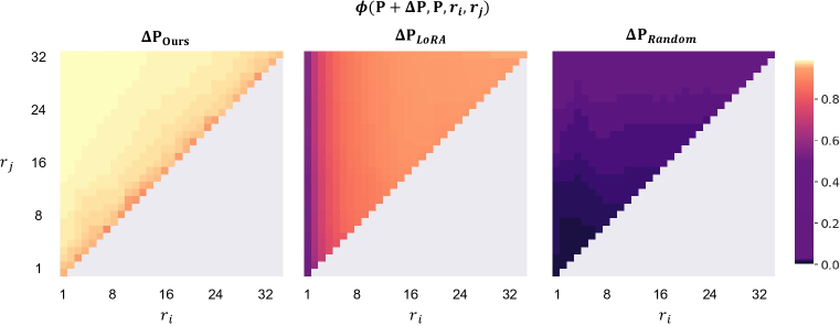
Figure 10: Subspace similarity between $P+\Delta P$ and $P$. The similarity $\phi(P+\Delta P_{Ours},P,r_{i},r_{j})$ between our updated parameter matrix and the pretrained parameter matrix achieves a similarity larger than 96% across different dimensions of the subspace $(r_{i},r_{j})$. The results indicare the learned sparse parameter matrix $\Delta P$ of our model keeps the prior information in the pretrained parameters $P$ well.

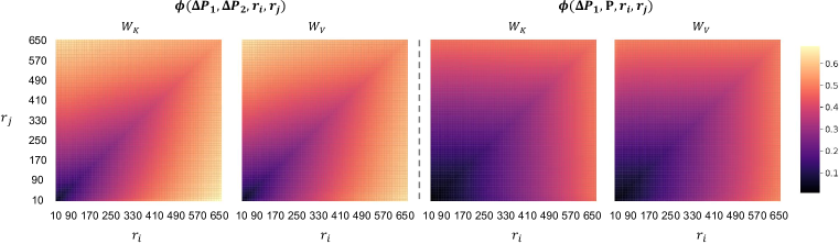
Figure 11: Subspace similarity between $\Delta P_{1}$ and $\Delta P_{2}$ under thresholds $2e-3$ and $8e-4$. The total similarity between their learned matrices exceeds $60\%$ (when $r$ is around 650), compared to only $40\%$ similarity between $\Delta P_{1}$ and the pre-trained weights $P$, demonstrating the learned matrices from different thresholds learn similar task-specific knowledge, while emphasizing different directions (relative smaller similarity when $r$ is small).

The Correlation between $P+\Delta P$ and $P$. We aim to further understand whether our learned parameter matrix $\Delta P_{Ours}$ disrupts the information in the original parameter space (spanned by the pretrained weights $P$), which may lead to overfitting and loss of prior information. To analyze the preservation of prior information, we calculate the correlation between the final updated parameter matrix $(P+\Delta P)$ and the pretrained weights $P$. Specifically, we calculate the similarity between the subspaces of $(P+\Delta P)$ and $P$. We decompose $(P+\Delta P)$ and $P$ using Singular Value Decomposition (SVD) to obtain the left-singular unitary matrices $U$, and examine the similarity between the subspaces spanned by the first $r_{i}$ singular vectors of $U_{P+\Delta P}$ and the first $r_{j}$ singular vectors of $U_{P}$. We quantify the subspace similarity using the normalized subspace similarity based on the Grassmann distance (Hu et al., 2021):

$$\phi(P_{1},P_{2},r_{i},r_{j})=\frac{\|U_{1}^{r_{i}T}U_{2}^{r_{j}}\|_{F}^{2}}{min(r_{i},r_{j})}\in[0,1],$$ (9)

$$\text{where }U_{k}\Sigma_{k}V_{K}^{T}=SVD(P_{k}),k=\{1,2\}.$$

We calculate the similarity between the pre-trained parameter matrix $P$ and the updated parameter matrices obtained from three approaches: 1) our model $(P+\Delta P_{Ours})$, 2) LoRA $(P+\Delta P_{LoRA})$, and 3) a random parameter matrix added to the pre-trained parameters $(P+\Delta P_{Random})$. The results are shown in Fig. 10. As a reference, the subspace similarity $\phi(P+\Delta P_{Random},P,r_{i},r_{j})$ of randomly updated parameters approaches zero across different dimensions $r_{j}$ and $r_{j}$, indicating random weights will destroy the prior information in the pre-trained weights absolutely. In contrast, the similarity $\phi(P+\Delta P_{Ours},P,r_{i},r_{j})$ between our learned parameter matrix added to the pre-trained parameters and the original parameter matrix exceeds $96\%$ across different subspace dimensions $(r_{i},r_{j})$, indicating that our learned parameter matrix effectively preserves the information in the original parameter matrix. In addition, compared to the parameter matrix $(P+\Delta P_{Lora})$ updated by LoRA, our updated parameter matrix $(P+\Delta P_{Ours})$ shows greater subspace similarity with the pre-trained parameters $P$, demonstrating that our model’s learned sparse parameter matrix better preserves the prior information of the pre-trained parameters, effectively avoiding model overfitting. Combining this with the conclusions from the previous section, we can further conclude that Our model can learn more task-specific knowledge, while more effectively preserving the prior information of the pre-trained parameter matrix than LoRA.

The Correlation between $\Delta P$ under Different Thresholds. We further investigate the relationship between the learned parameter matrices $\Delta P$ under different thresholds. Our experiments focus on the matrices for Key $W_{K}$ and Value $W_{V}$ from the medium block’s attention modules in SD1.5. In this experiments, we select two thresholds, $2e-3$ and $8e-4$ (corresponding to $\Delta P_{1}$ and $\Delta P_{2}$), and compute the similarity of their subspaces using Eq. (9). For comparison, we also calculate the similarity between the parameter matrix $\Delta P_{1}$ learned with a threshold of $2e-3$ and the pre-trained parameter matrix $P$. The results are shown in Fig. 11. It can be observed that the overall similarity between the parameter matrices learned under the two thresholds exceeds $60\%$ (peaking at around $r=650$), indicating that the knowledge learned under different thresholds is roughly similar, but with different emphases (lower similarity at smaller $r$). In contrast, the similarity between $\Delta P_{1}$ and the pre-trained parameters $P$ is consistently below $40\%$. The higher similarity between $\Delta P_{1}$ and $\Delta P_{2}$ suggests that the learned parameter matrices from different thresholds indeed capture similar task-specific knowledge, which supports the feasibility of fine-tuning the model with fewer parameters.

6 Conclusion

In this paper, we propose SaRA, a novel parameter-efficient fine-tuning method, which makes full use of the ineffective parameters with the smallest absolute values in the pre-trained model. We propose a nuclear norm-based low-rank loss to constrain the rank of the learned sparse matrices, thereby avoiding model overfitting. Moreover, we design a progressive parameter adjustment strategy, which can further improve the effectiveness of the fine-tuned parameters. Finally, we propose a novel unstructural backpropagation method, largely saving the memory cost during parameter fine-tuning, which can also reduce the memory costs for other selective PEFT methods. Extensive experiments demonstrate the effectiveness of our method, which achieves the best fitting capability while keeping the prior information of the pre-trained model well. In addition, we efficiently encapsulate our method such that it can be implemented by only modifying one line of code, which largely enhances the ease of use and adaptability of the code for other models and tasks.

Appendix A More Implementation Details

Visual-Linguistic Harmony Index (VLHI). We propose VLHI to evaluate both the style and the generalization of each PEFT method, by balancing FID and CLIP Score. For a group of FIDs $\{FID_{i}\}_{i=1}^{n}$ and CLIP Scores $\{CLIP_{i}\}_{i=1}^{n}$, we compute the normalized FID and CLIP Score as VLHI:

$$VLHI_{i}=\frac{\max(\{FID_{i}\}_{i=1}^{n})-FID_{i}}{\max(\{FID_{i}\}_{i=1}^{n})-\min(\{FID_{i}\}_{i=1}^{n})}+\frac{CLIP_{i}-\min(\{CLIP_{i}\}_{i=1}^{n})}{\max(\{CLIP_{i}\}_{i=1}^{n})-\min(\{CLIP_{i}\}_{i=1}^{n})}$$ (10)

For downstream dataset fine-tuning experiments, we regard the methods in one Stable Diffusion version and one dataset as a group.

Training Details. We use AdamW (Loshchilov et al., 2017) optimizer to train the methods for 5000 iterations with batch size 4, with a cosine learning rate scheduler, where the initial learning rate $lr$ is calculated corresponds to the thresholds $\theta_{t}$: $lr=10^{-3}\times e^{-350\theta_{t}}$ (refer to Sec. 14). For the training images and labeled captions, we recaption them by adding a prefix ‘$name\,style,\,$’ ($name$ corresponds to the dataset name) before each caption, which is a common trick in fine-tuning Stable Diffusion models to a new domain.

Appendix B More comparison results

In the downstream dataset fine-tuning experiments of the main paper, we show the qualitative results on Stable Diffusion 1.5 with resolution 512. In this section, we show more results on Stable Diffusion 2.0 and 3.0 with resolutions 768 and 1,024. The results from Stable Diffusion 2.0 and 3.0 are shown in Fig. 12 and Fig. 13 respectively. It can be seen that our model generates images that contain most of the features in the target domain and are well consistent with the given prompts.

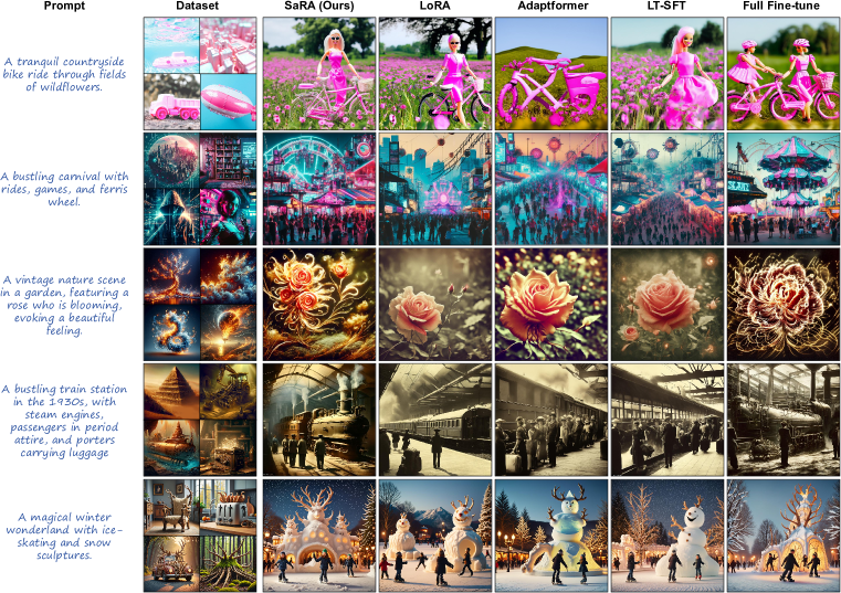
Figure 12: Comparison results between different PEFT methods on Stable Diffusion 2.0.

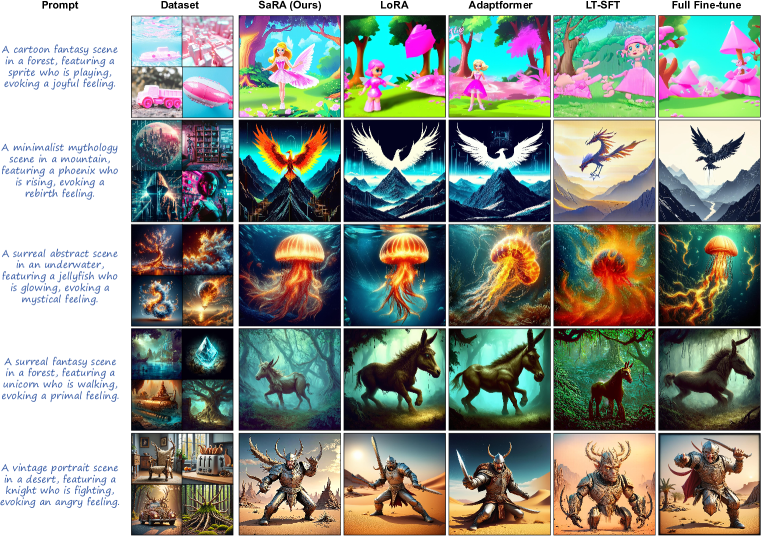
Figure 13: Comparison results between different PEFT methods on Stable Diffusion 3.0.

Appendix C Hyperparameter Analysis

In this section, we conduct experiments on different hyperparameters in our model: learning rate, progressive iteration (the iteration for progressive parameter adjustment), and the weight for rank loss $\lambda_{rank}$. We chose Stable Diffusion 1.5 and Expedition dataset for the following experiments (if not specified, the threshold $\theta_{t}=2e-3$) and evaluated the results by FID, CLIP Score, and VLHI.

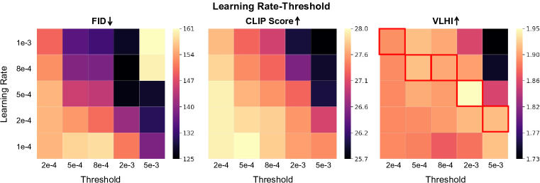
Figure 14: The comparison results on different learning rates and thresholds. The model with a larger threshold should employ a larger learning rate to learn the target-domain information well (red boxes indicate the best results).

Learning Rates and Thresholds. We first investigate the two most critical hyperparameters: learning rate and threshold. We selected learning rates $\{1e-4,2e-4,5e-4,8e-4,1e-3\}$ and thresholds $\{2e-4,5e-4,8e-4,2e-3,5e-3\}$ for our experiments, resulting in a total of 25 models. The quantitative results are shown in Fig. 14. It can be observed that, for the same learning rate, as the threshold increases, the model’s FID gradually decreases while the CLIP Score gradually increases. This indicates that a larger learnable parameter set can learn more task-specific information, but is also more likely to lose pre-trained prior knowledge. For the same threshold, increasing the learning rate yields similar results. However, for relatively large thresholds (e.g., $5e-3$), a high learning rate (e.g., $8e-4$ and $1e-3$ in the figure) may cause the model training to collapse. Therefore, selecting an appropriate learning rate is crucial for achieving good results.

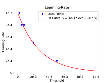
Figure 15: The fit curve of the best pairs of learning rate and threshold.

We further use the VLHI metric to analyze the performance of the models trained with different learning rates under various thresholds by balancing FID and CLIP scores, as shown in the third column in Fig. 14. The optimal learning rate for each threshold is marked with a red box. It can be seen that as the threshold increases, a gradually decreasing learning rate should be used to prevent severe overfitting. Conversely, as the threshold decreases, a larger learning rate should be employed to enhance the model’s ability to learn task-specific knowledge. In summary, there is a negative correlation between the learning rate and the threshold. To adaptively select an optimal learning rate, we fit an exponential function $f(x)=a\times e^{b}$ using the five data points shown in the figure. The resulting function for adaptively computing the learning rate for different thresholds is shown in Fig. 15. The curve fits the five data points well, and when the threshold approaches $0$, the learning rate is approximately $1e-3$, which does not result in an excessively high learning rate. Similarly, for larger thresholds (e.g., $1e-2$), the learning rate is around $3e-5$, comparable to the learning rate used in full fine-tuning, avoiding an excessively low learning rate. We do not consider even larger thresholds, as these parameters are highly effective in the model, and fine-tuning them would contradict the purpose of our method. Therefore, we derive a function to adaptively compute a good learning rate $Lr$ based on the threshold $\theta_{t}$:

$$Lr=10^{-3}\times e^{-350\theta_{t}}.$$ (11)

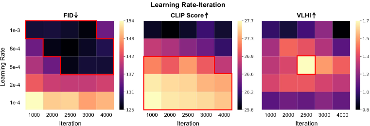
Figure 16: The comparison results on different learning rates and progressive iterations. A larger learning rate or progressive iteration improves the FID while sacrificing the CLIP Score.

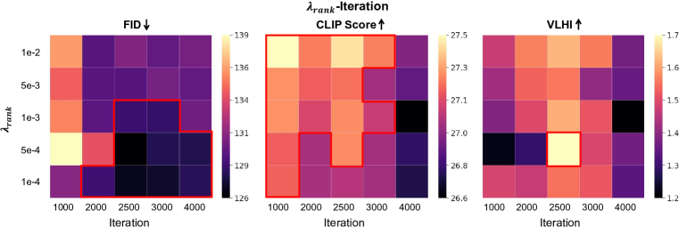
Figure 17: The comparison results on different weights $\lambda_{rank}$ for rank loss and progressive iterations. A larger $\lambda_{rank}$ improves the CLIP Score while sacrificing the FID.

Learning Rates and Progressive Iteration. We then study the effects of learning rate and progressive iteration (the iteration for progressive parameter adjustment) together. We train the models with learning rates $\{1e-4,2e-4,5e-4,8e-4,1e-3\}$ and progressive iteration $\{1000,2000,2500,3000,4000\}$, which forms 25 models in total. The quantitative results are shown in Fig. 16. For all the metrics (FID, CLIP Score, and VLHI), the brighter the color is, the better the model performs. It can be seen that, as the learning rate or progressive iteration grows, the model learns more task-specific knowledge (a better FID), while the CLIP score becomes worse. Therefore, we should balance both the learning rate and progressive iterations, where the model with learning rate $5e-4$ and progressive iteration $2000$ achieves the best VLHI, reaching both a good FID and CLIP Score.

$\lambda_{rank}$ and Progressive Iteration. We then analyze the influence of the weight for rank loss $\lambda_{rank}$ and progressive iteration at the same time. We train the models with $\lambda_{rank}$ $\{1e-4,5e-4,1e-3,5e-3,1e-2\}$ and progressive iteration $\{1000,2000,2500,3000,4000\}$, which constitutes 25 models in total. The quantitative results are shown in Fig. 17. It can be seen that as $\lambda_{rank}$ increases, the FID becomes worse while the CLIP Score performs better, demonstrating that $\lambda_{rank}$ helps the model keep the prior information in the pre-trained weights, but with a less effect in fitting the target domain. Therefore, to simultaneously reach a relatively good FID and CLIP Score, we choose $\lambda_{rank}=5e-3$ with progressive iteration $2500$, which results in the best VLHI.

Figure 18: Subspace similarity between $\Delta P$ and $P$ under different thresholds.

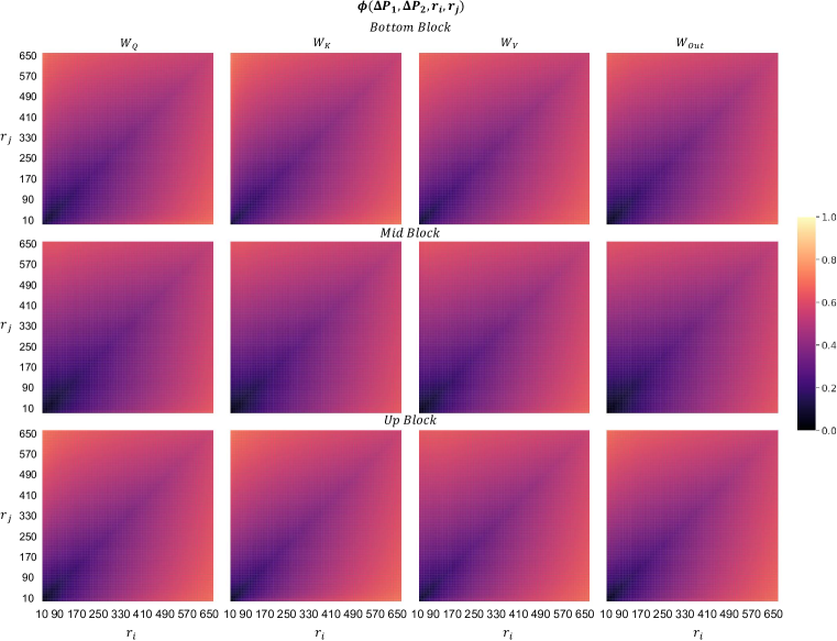
Figure 19: Subspace similarity between $\Delta P$ from threshold $\theta_{t}=2e-3$ (50M parameters) and $\theta_{t}=8e-4$ (20M parameters), in different attention layers, where the x-axis and y-axis represent $\theta_{t}=2e-3$ and $\theta_{t}=8e-4$ respectively. The subspace similarity across different layers exhibits consistent behavior, demonstrating that the knowledge learned by $\Delta P$ remains invariant across layers and modules, indicating strong robustness.

Appendix D More Analysis on the learned weight matrix $\Delta P$

The Correlation between $\Delta P$ and $P$ under Different Thresholds. We compute the subspace similarity between the learned matrices $Delta_{P}$ under different thresholds and the pre-trained weights $P$ by Eq. (6) of the main paper. The results are shown in Fig. 18. It demonstrates that $\Delta P$ does not contain the top singular directions of W, since the overall similarity between the singular directions in the learned matrices $\Delta P$ and the top 32 directions of $P$ is barely around $4\%$. And it further validates that the matrices $\Delta P$ contain more task-specific information rather than repeating the directions that are already emphasized in the pre-trained weights. Moreover, by comparing the $\Delta P$ from different thresholds, we can find that as the thresholds grow, the subspace similarity between $\Delta P$ and $P$ becomes smaller, indicating that a larger threshold can learn more task-specific information, therefore a large threshold can contribute to a better FID as shown in Tab. 1.

More Analysis on $\Delta P$ from Different Layers. In the main paper, we have analyzed the subspace similarity between the learned matrices $\Delta P$ from different thresholds, and concluded that the matrices from different thresholds learn similar task-specific knowledge, but emphasize different directions. To further validate this conclusion, we conduct more quantitative analysis between different thresholds ($\theta_{t}=2e-3$ and $8e-4$) from the attention layers in the bottom, medium, and up blocks. Moreover, we take all the learnable matrices in the attention module into consideration, including the Query, Key, Value, and FFN matrices (corresponds to $W_{Q}$, $W_{K}$, $W_{V}$, and $W_{Out}$ respectively). The results can be referred to in Fig. 19 the x-axis and y-axis represent $\theta_{t}=2e-3$ and $\theta_{t}=8e-4$ respectively., where the heatmaps show almost the same color and distributions, indicating that our conclusion is consistent for the learned matrices from different modules and different attention layers.

Further Analysis of $\Delta P$ across Different Threshold Pairs. In the main paper, we analyzed the subspace similarity between the learned matrices $\Delta P$ from thresholds of $2e-3$ and $8e-4$, concluding that the learned matrices from different thresholds capture similar task-specific knowledge while emphasizing different directions. In this section, we extend our quantitative analysis to additional threshold pairs: $(2e-3,8e-4)$, $(2e-3,2e-4)$, and $(8e-4,2e-4)$. We consider all learnable matrices in the attention module, including the Query, Key, Value, and FFN matrices (corresponding to $W_{Q}$, $W_{K}$, $W_{V}$, and $W_{Out}$, respectively). The results are presented in Fig. 20. The subspace similarity between the thresholds $(2e-3,2e-4)$ is lower than that of $(2e-3,8e-4)$ and $(8e-4,2e-4)$, suggesting that matrices learned from a closer threshold pair exhibits greater subspace similarity and acquire more similar knowledge.

Figure 20: Subspace similarity between $\Delta P$ across different threshold pairs: $(2e-3,8e-4)$, $(2e-3,2e-4)$, and $(8e-4,2e-4)$ (from top to bottom).

References

- Aghajanyan et al. (2020) Armen Aghajanyan, Luke Zettlemoyer, and Sonal Gupta. Intrinsic dimensionality explains the effectiveness of language model fine-tuning. arXiv preprint arXiv:2012.13255, 2020.
- Ansell et al. (2021) Alan Ansell, Edoardo Maria Ponti, Anna Korhonen, and Ivan Vulić. Composable sparse fine-tuning for cross-lingual transfer. arXiv preprint arXiv:2110.07560, 2021.
- Blattmann et al. (2023) Andreas Blattmann, Robin Rombach, Huan Ling, Tim Dockhorn, Seung Wook Kim, Sanja Fidler, and Karsten Kreis. Align your latents: High-resolution video synthesis with latent diffusion models. In Proceedings of the IEEE/CVF Conference on Computer Vision and Pattern Recognition, pp. 22563–22575, 2023.
- Chen et al. (2022) Shoufa Chen, Chongjian Ge, Zhan Tong, Jiangliu Wang, Yibing Song, Jue Wang, and Ping Luo. Adaptformer: Adapting vision transformers for scalable visual recognition. Advances in Neural Information Processing Systems, 35:16664–16678, 2022.
- Deng et al. (2009) Jia Deng, Wei Dong, Richard Socher, Li-Jia Li, Kai Li, and Li Fei-Fei. Imagenet: A large-scale hierarchical image database. In 2009 IEEE conference on computer vision and pattern recognition, pp. 248–255. Ieee, 2009.
- Ding et al. (2023) Ning Ding, Xingtai Lv, Qiaosen Wang, Yulin Chen, Bowen Zhou, Zhiyuan Liu, and Maosong Sun. Sparse low-rank adaptation of pre-trained language models. arXiv preprint arXiv:2311.11696, 2023.
- Edalati et al. (2022) Ali Edalati, Marzieh Tahaei, Ivan Kobyzev, Vahid Partovi Nia, James J Clark, and Mehdi Rezagholizadeh. Krona: Parameter efficient tuning with kronecker adapter. arXiv preprint arXiv:2212.10650, 2022.
- Esser et al. (2024) Patrick Esser, Sumith Kulal, Andreas Blattmann, Rahim Entezari, Jonas Müller, Harry Saini, Yam Levi, Dominik Lorenz, Axel Sauer, Frederic Boesel, et al. Scaling rectified flow transformers for high-resolution image synthesis. In Forty-first International Conference on Machine Learning, 2024.
- Frankle & Carbin (2018) Jonathan Frankle and Michael Carbin. The lottery ticket hypothesis: Finding sparse, trainable neural networks. arXiv preprint arXiv:1803.03635, 2018.
- Gal et al. (2022) Rinon Gal, Yuval Alaluf, Yuval Atzmon, Or Patashnik, Amit H Bermano, Gal Chechik, and Daniel Cohen-Or. An image is worth one word: Personalizing text-to-image generation using textual inversion. arXiv preprint arXiv:2208.01618, 2022.
- Guo et al. (2020) Demi Guo, Alexander M Rush, and Yoon Kim. Parameter-efficient transfer learning with diff pruning. arXiv preprint arXiv:2012.07463, 2020.
- Guo et al. (2023) Yuwei Guo, Ceyuan Yang, Anyi Rao, Yaohui Wang, Yu Qiao, Dahua Lin, and Bo Dai. Animatediff: Animate your personalized text-to-image diffusion models without specific tuning. arXiv preprint arXiv:2307.04725, 2023.
- Han et al. (2024) Zeyu Han, Chao Gao, Jinyang Liu, Sai Qian Zhang, et al. Parameter-efficient fine-tuning for large models: A comprehensive survey. arXiv preprint arXiv:2403.14608, 2024.
- Hayou et al. (2024) Soufiane Hayou, Nikhil Ghosh, and Bin Yu. Lora+: Efficient low rank adaptation of large models. arXiv preprint arXiv:2402.12354, 2024.
- Heusel et al. (2017) Martin Heusel, Hubert Ramsauer, Thomas Unterthiner, Bernhard Nessler, and Sepp Hochreiter. Gans trained by a two time-scale update rule converge to a local nash equilibrium. Advances in neural information processing systems, 30, 2017.
- Ho et al. (2020) Jonathan Ho, Ajay Jain, and Pieter Abbeel. Denoising diffusion probabilistic models. Advances in neural information processing systems, 33:6840–6851, 2020.
- Houlsby et al. (2019) Neil Houlsby, Andrei Giurgiu, Stanislaw Jastrzebski, Bruna Morrone, Quentin De Laroussilhe, Andrea Gesmundo, Mona Attariyan, and Sylvain Gelly. Parameter-efficient transfer learning for nlp. In International conference on machine learning, pp. 2790–2799. PMLR, 2019.
- Hu et al. (2021) Edward J Hu, Yelong Shen, Phillip Wallis, Zeyuan Allen-Zhu, Yuanzhi Li, Shean Wang, Lu Wang, and Weizhu Chen. Lora: Low-rank adaptation of large language models. arXiv preprint arXiv:2106.09685, 2021.
- Karras et al. (2017) Tero Karras, Timo Aila, Samuli Laine, and Jaakko Lehtinen. Progressive growing of gans for improved quality, stability, and variation. arXiv preprint arXiv:1710.10196, 2017.
- Karras et al. (2019) Tero Karras, Samuli Laine, and Timo Aila. A style-based generator architecture for generative adversarial networks. In Proceedings of the IEEE/CVF conference on computer vision and pattern recognition, pp. 4401–4410, 2019.
- Kawar et al. (2023) Bahjat Kawar, Shiran Zada, Oran Lang, Omer Tov, Huiwen Chang, Tali Dekel, Inbar Mosseri, and Michal Irani. Imagic: Text-based real image editing with diffusion models. In Proceedings of the IEEE/CVF Conference on Computer Vision and Pattern Recognition, pp. 6007–6017, 2023.
- Lei et al. (2023) Tao Lei, Junwen Bai, Siddhartha Brahma, Joshua Ainslie, Kenton Lee, Yanqi Zhou, Nan Du, Vincent Zhao, Yuexin Wu, Bo Li, et al. Conditional adapters: Parameter-efficient transfer learning with fast inference. Advances in Neural Information Processing Systems, 36:8152–8172, 2023.
- Li et al. (2022) Junnan Li, Dongxu Li, Caiming Xiong, and Steven Hoi. Blip: Bootstrapping language-image pre-training for unified vision-language understanding and generation. In International conference on machine learning, pp. 12888–12900. PMLR, 2022.
- Liang et al. (2021) Tailin Liang, John Glossner, Lei Wang, Shaobo Shi, and Xiaotong Zhang. Pruning and quantization for deep neural network acceleration: A survey. Neurocomputing, 461:370–403, 2021.
- Liao et al. (2023) Baohao Liao, Yan Meng, and Christof Monz. Parameter-efficient fine-tuning without introducing new latency. arXiv preprint arXiv:2305.16742, 2023.
- Loshchilov et al. (2017) Ilya Loshchilov, Frank Hutter, et al. Fixing weight decay regularization in adam. arXiv preprint arXiv:1711.05101, 5, 2017.
- Mahabadi et al. (2021) Rabeeh Karimi Mahabadi, Sebastian Ruder, Mostafa Dehghani, and James Henderson. Parameter-efficient multi-task fine-tuning for transformers via shared hypernetworks. arXiv preprint arXiv:2106.04489, 2021.
- Mou et al. (2024) Chong Mou, Xintao Wang, Liangbin Xie, Yanze Wu, Jian Zhang, Zhongang Qi, and Ying Shan. T2i-adapter: Learning adapters to dig out more controllable ability for text-to-image diffusion models. In Proceedings of the AAAI Conference on Artificial Intelligence, volume 38, pp. 4296–4304, 2024.
- Pfeiffer et al. (2020) Jonas Pfeiffer, Aishwarya Kamath, Andreas Rücklé, Kyunghyun Cho, and Iryna Gurevych. Adapterfusion: Non-destructive task composition for transfer learning. arXiv preprint arXiv:2005.00247, 2020.
- Poole et al. (2022) Ben Poole, Ajay Jain, Jonathan T Barron, and Ben Mildenhall. Dreamfusion: Text-to-3d using 2d diffusion. arXiv preprint arXiv:2209.14988, 2022.
- Radford et al. (2021) Alec Radford, Jong Wook Kim, Chris Hallacy, Aditya Ramesh, Gabriel Goh, Sandhini Agarwal, Girish Sastry, Amanda Askell, Pamela Mishkin, Jack Clark, et al. Learning transferable visual models from natural language supervision. In International conference on machine learning, pp. 8748–8763. PMLR, 2021.
- Rombach et al. (2022) Robin Rombach, Andreas Blattmann, Dominik Lorenz, Patrick Esser, and Björn Ommer. High-resolution image synthesis with latent diffusion models. In Proceedings of the IEEE/CVF conference on computer vision and pattern recognition, pp. 10684–10695, 2022.
- Ruiz et al. (2023) Nataniel Ruiz, Yuanzhen Li, Varun Jampani, Yael Pritch, Michael Rubinstein, and Kfir Aberman. Dreambooth: Fine tuning text-to-image diffusion models for subject-driven generation. In Proceedings of the IEEE/CVF Conference on Computer Vision and Pattern Recognition, pp. 22500–22510, 2023.
- Sun et al. (2023) Jingxiang Sun, Bo Zhang, Ruizhi Shao, Lizhen Wang, Wen Liu, Zhenda Xie, and Yebin Liu. Dreamcraft3d: Hierarchical 3d generation with bootstrapped diffusion prior. arXiv preprint arXiv:2310.16818, 2023.
- Sung et al. (2021) Yi-Lin Sung, Varun Nair, and Colin A Raffel. Training neural networks with fixed sparse masks. Advances in Neural Information Processing Systems, 34:24193–24205, 2021.
- Valipour et al. (2022) Mojtaba Valipour, Mehdi Rezagholizadeh, Ivan Kobyzev, and Ali Ghodsi. Dylora: Parameter efficient tuning of pre-trained models using dynamic search-free low-rank adaptation. arXiv preprint arXiv:2210.07558, 2022.
- Van Le et al. (2023) Thanh Van Le, Hao Phung, Thuan Hoang Nguyen, Quan Dao, Ngoc N Tran, and Anh Tran. Anti-dreambooth: Protecting users from personalized text-to-image synthesis. In Proceedings of the IEEE/CVF International Conference on Computer Vision, pp. 2116–2127, 2023.
- Wang et al. (2022) Yaqing Wang, Sahaj Agarwal, Subhabrata Mukherjee, Xiaodong Liu, Jing Gao, Ahmed Hassan Awadallah, and Jianfeng Gao. Adamix: Mixture-of-adaptations for parameter-efficient model tuning. arXiv preprint arXiv:2205.12410, 2022.
- Wang et al. (2024) Zhengyi Wang, Cheng Lu, Yikai Wang, Fan Bao, Chongxuan Li, Hang Su, and Jun Zhu. Prolificdreamer: High-fidelity and diverse text-to-3d generation with variational score distillation. Advances in Neural Information Processing Systems, 36, 2024.
- Watson (1992) G Alistair Watson. Characterization of the subdifferential of some matrix norms. Linear Algebra Appl, 170(1):33–45, 1992.
- Yang et al. (2023) Adam X Yang, Maxime Robeyns, Xi Wang, and Laurence Aitchison. Bayesian low-rank adaptation for large language models. arXiv preprint arXiv:2308.13111, 2023.
- Ye et al. (2023) Hu Ye, Jun Zhang, Sibo Liu, Xiao Han, and Wei Yang. Ip-adapter: Text compatible image prompt adapter for text-to-image diffusion models. arXiv preprint arXiv:2308.06721, 2023.
- Zhang et al. (2023a) Lvmin Zhang, Anyi Rao, and Maneesh Agrawala. Adding conditional control to text-to-image diffusion models. In Proceedings of the IEEE/CVF International Conference on Computer Vision, pp. 3836–3847, 2023a.
- Zhang et al. (2023b) Qingru Zhang, Minshuo Chen, Alexander Bukharin, Pengcheng He, Yu Cheng, Weizhu Chen, and Tuo Zhao. Adaptive budget allocation for parameter-efficient fine-tuning. In International Conference on Learning Representations. Openreview, 2023b.