The resistivity of rare earth impurities diluted in Lanthanum (Part I)

Abstract

In this work we study the temperature independent resistivity of rare-earth magnetic (Gd, Tb, Dy) and non-magnetic (Lu) impurities diluted in dhcp Lanthanum. We considered a two-band system where the conduction is entirely due to $s$-electrons while the screening of the charge difference induced by the impurity is made by the $d$-electrons. We obtain an expression of the resistivity using the $T$-matrix formalism from the Dyson equation. As the electronic properties depend strongly on the band structure, we have considered two types of bands structure, a “parabolic” band and a more realistic one calculated by first principles with VASP. We verify that the exchange parameters appearing as cross products strongly affect the magnitude of the spin resistivity term; And that the role of the band structure in resonant scattering or virtual bound states, depends on the band structure. Our study, also includes the influence of the translational symmetry breaking and the excess charge introduced by the rare-earth impurity on the resitivity.

1 Introduction

We have extended the expression of the temperature independent resistivity, $R$, associated to a rare earth impurity of Gd, Tb, Dy and Lu, embebbed in a transition metal like host obtained first by Troper and Gomes [1]. One has a two-band paramagnetic metallic system ($s-$ and $d-$character bands, non-hybridized for simplicity), coupled via usual exchange interactions $J^{(s)}$ and $J^{(d)}$ to the local $4f$-spin, associated to a magnetic rare earth impurity. We have assumed that the conduction is entirely due to $s$-electrons and that the screening of the charge difference induced by the impurities is made by the $d$-electrons. The degeneracy of the d-band may be included straightforwardly, considering the usual approximation of five identical subbands. In addition to [1] here we take into account two main charge effects introduced by the impurities, namely (i) charge difference between impurity - host, and (ii) the translational symmetry breaking, which leads to a non-local charge potential[2]. Moreover, we consider also in a phenomenologycal way, the effect of the volume difference between impurity and host [3]. In the case of “magnetic” rare earth impurities, we have also to consider the presence of a spin dependent potential, which will be treated in first order perturbation theory, as usual[4]. In the derivation of the temperature independent resistivity we have assumed that the magnetic impurity, placed at the origin, contributes with two sources of scattering, the spin independent potential, $R_{0}$, which arises from the charge difference introduced by the impurity, neglecting the intra s-band scattering, $V_{ss}$, the potential scattering through d-d scattering, $V_{dd}$ which was calculated via an extended Freidel sum rule, and impurity-induced s-d mixing as $V_{sd}$. Then, from the expression of $R$ in eq.(1) is be expressed as,

$$R(\epsilon)=R_{0}(\epsilon)+\pi Ac\rho_{s}(\epsilon)S_{0}(S_{0}+1)\left(J^{(s)}\right)^{2}\times\left\{1+\theta(\epsilon,|V_{sd}|^{2})\right\},$$ (1)

In (1) $A$ is a constant which depends on the characteristics of the $s-$Fermi surface of the host; $c$ is the concentration of impurities diluted in the host; the spin scattering term produced by the conduction electrons which are coupled to the impurity spin, $S_{0}$, through $k$-independent exchange interactions $J_{s}$ and $Jd$; and the function $\theta(\epsilon;|V_{sd}|^{2})$ which describes the combined effect of charge potential and spin dependent scattering in the departures of De-Gennes Friedel resistivity, $R_{DG-F}=\pi Ac(J^{(s)})^{2}S_{0}(S_{0}+1)$ which corresponds to neglecting the impurity charge scattering potential. First, we discuss the role of the band structure in resonant scattering (virtual bound states) adopting two types of density of states, a “ parabolic ” model and a more realistic band structure calculated with VASP. The rare earth impurity is assumed to be a “spherically symmetric rare earth”. Consequently, effects like skew scattering (connected to spin-orbit coupling) and crystal field splitting, are entirely disregarded in this work. In this sense, our calculation intends to apply properly only for $Gd$ impurity in transition like hosts with total spin $S_{0}(Gd)=7/2$. However one can consider also $Tb$ and $Dy$ impurities, with $L\neq 0$, by substituting $S_{0}$ by $(g_{j}-1)J_{0}=S_{0}^{eff}$ , where $(g_{j}-1)$ called the De-Gennes factor, is the projection of the spin $S_{0}$ on the total angular momentum $J_{0}$ of the $Tb$ or $Dy$ impurities. So, $S_{0}(Gd)=7/2$, $S^{eff}_{0}(Tb)=6/2$ and $S^{eff}_{0}(Dy)=5/2$. Notice that $S_{0}$ and $S^{eff}_{0}$ are good quantum numbers and they arise from Hund’s rules. An essential characteristic of a rare earth placed in a transition metal host as Lanthanum, is the existence of a charge difference between host and impurity (which is trivalent in general). The simultaneous existence of spin and charge potential scattering is the signature of the behavior of such impurities in transition metal hosts. The role of the band structure in resonant scattering (virtual bound states) is sudied adopting a realistic band structure and calculate the susceptibilities involved. By changing in the band structure the position of the Fermi level, in order to scan the neighborhood of the top of the band, the regions of narrow peaks, etc., the role of these details is discussed properly in present calculations. In Summary, we study the dependence of the temperature-independent resistivity on the band structure of the 5d-serie Host. We start from the case of diluted Lanthanum alloys containing rare earth impurities such as Gd, Tb, Dy and Lu. With this purpose, we use two types of models for the band structure, one known as a “parabolic” type band and another more realistic one derived from first-principles calculations using the VASP code [5]-[8]. Our results have corroborated the strong dependence of the band structure on the Resistivity and therefore on the shape of the DOS used. As evidence of this conclusion, we have observed that:

1. Our expression of the temperature independent resistivity in terms of the hybridization charge potential, $|V_{sd}|^{2}$, changes drastically if we use the parabolic or the realistic model for the DOS.

2. Also, we study the exact form of the resistivity, $R=R(\epsilon,|V_{sd}|^{2})$, and the approximate case, $R_{app.}=|V_{sd}|^{2}R(\epsilon)$, up to first order in $|V_{sd}|^{2}$. We notice that, with the DOS-Moriya the interval of $|V_{sd}|^{2}$ values in which $R\simeq R_{app.}$ is smaller than for the realistic DOS. While, for the last case, the $R_{app.}$ is practicaly equal in the whole interval of $V_{sd}$ considered.

3. As per we have observed in 2., for the case of the realistic DOS we have the possibility of separating the s-d charge effects from the d-d ones assuming the approximation up to first order in $|V_{sd}|^{2}$. These results will be presented in a next work.

4. Given the important consequences of the DOS on the temperature independent of the temperature, $R$, we have performed the systematic for transition metal hosts belong the 5d series as: Hf, Ta, W, Re, Ir, Os, Pt and Au. These results will be also presented in a future work.

This work is organized as follows, In Section 2 we present the two-band model in order to obtain an approximated expression of the temperature independent resistivity summarized in Section 3. Section 4, describes the computational procedure and the performed convergence test in order to obtain the energy and the k-mesh from DFT calculations with VASP for both, the primitive and the supercell, respectively. Section 5.1 summarizes present results of the band structure calculations from the previously relaxed La structure pf dhcp-La, the critical potential and the calculated resistivity of de impurities (Gd, Tb, Dy an Lu) diluted in dhcp-La using the “parabolic” model and the one based on DFT calculations for the s- and d- density of states of Lanthanum. We use the approximation of homothetic d-band $\epsilon_{dk}=\alpha\epsilon_{sk}$, wher $\alpha$ é is a fenomenological parameter which corresponds to the relation of the $s(p)$-$d$ electron effective masses and $\epsilon_{\lambda k}$ is the dispersion relation of the $\lambda$- elétrons (with $\lambda=s,d$). We have described the interband effects though a one body hubridization term, different from the usual many bodies approach. We consider the hybridization described in the independent approximation of the wave vector $\vec{k}$. In Section 6 some conclusions are presented. Also, we include two Appendix sections in order of complete the description of our system.

2 The two-band Hamiltonian model

We consider a two-band model for the host assuming that, for simplicity, s- and d-bands are not hybridized. As conduction is due almost exclusively to the s-electrons, we restrict our derivation of a Dyson-like equation to the one-electron $s-s$ perturbed propagators in terms of the host metal. This equation is valid to all orders in perturbation theory within the accuracy of Nagaokaś decoupling scheme. In our model the full Hamiltonian is written as in Ref.[1],

$$H=H_{0}^{(s,d)}+H_{I}^{q}+H_{I}^{\tau}+H_{I}^{\vec{S}_{0}},$$ (2)

In (2), the pure host is described by the following Hamiltonian:

$$H_{0}^{(s,d)}=\sum_{i,j,\sigma}t_{ij}^{(s)}c_{i\sigma}^{\dagger}c_{j\sigma}+\sum_{i,j,\sigma}t_{ij}^{(d)}d_{i\sigma}^{\dagger}d_{j\sigma},$$ (3)

with $t_{ij}^{(\lambda)}$ the transfer integral of $\lambda$-electrons between the host’s sites $i$ and $j$. On the other hand a magnetic impurity, placed at the origin, contributes with two sources of scattering, the spin independent potential, which arises from the charge difference introduced by the impurity, $V_{ss}$, the potential scattering through d-d scattering and impurity-induced s-d mixing as,

$$H_{I}^{q}=V_{dd}\sum_{\sigma}n_{0\sigma}^{(d)}+\sum_{\sigma}\left\{V_{sd}c_{0\sigma}^{\dagger}d_{0\sigma}+V_{ds}d_{0\sigma}^{\dagger}c_{0\sigma}\right\};$$ (4)

and the spin scattering produced by the conduction electrons which are coupled to the impurity spin through $k,k^{\prime}$-independent exchange interactions. The corresponding Hamiltonian is,

$$H_{I}^{\vec{S}_{0}}=J^{(s)}\vec{\sigma}^{(s)}.\vec{S}_{0}+J^{(d)}\vec{\sigma}^{(d)}.\vec{S}_{0},$$ (5)

where the constants $J^{(s,d)}$, are the $s,d$-electrons exchange integrals, respectively. $\vec{S}_{0}$ is the local impurity spin with components $a_{i}=c_{i},d_{i}$,

$$\sigma^{z}_{i}=a^{\dagger}_{i\uparrow}a_{i\uparrow}-a^{\dagger}_{i\downarrow}a_{i\downarrow},\,\,\sigma^{+}_{i}=a^{\dagger}_{i\uparrow}a_{i\downarrow},\,\,\sigma^{-}_{i}=a^{\dagger}_{i\downarrow}a_{i\uparrow}.$$ (6)

We extend the Hamiltonian in Ref.[1] by including two main charge effects introduced by the impurities namely, the translational symmetry breaking,

$$H_{I}^{\tau}=\tau\sum_{m\neq 0,\sigma}\left\{t_{0m}^{(d)}d_{0\sigma}^{\dagger}d_{m\sigma}+t_{m0}^{(d)}d_{m\sigma}^{\dagger}d_{0\sigma}\right\};$$ (7)

and the volume difference between impurity ($\Omega^{I}$) and host ($\Omega$), is incorporated in the effective charge difference,

$$\Delta Z^{\prime}=\Delta Z-\frac{\Omega^{I}-\Omega}{\Omega}=\Delta Z-\frac{\delta v}{\Omega},$$ (8)

with $\Delta Z$ calculated as,

$$\Delta Z=\frac{2}{\pi}\tan^{-1}\frac{\pi|V_{dd}(\omega)|\rho_{d}(\omega)}{1-|V_{dd}(\omega)|g_{00}^{dd(R)}(\omega)},$$ (9)

with $\Delta Z$ and $\Delta Z^{\prime}$ the real and effective difference of charge between impurity and host elements. In the absence of spin scattering the solution, in terms of the $T$-matrix and the perfect lattice propagators, $P^{\lambda\lambda}_{ij}$ (with $\lambda=s,d$), is given by

$$G_{ij}^{ss}(\omega)=P_{ij}^{ss}(\omega)+2\pi P_{i0}^{ss}(\omega)T^{ss}(\omega)P_{0j}^{ss}(\omega),$$ (10)

and

$$G_{ij}^{ds}(\omega)=2\pi P_{i0}^{dd}(\omega)T^{ds}(\omega)P_{0j}^{ss}(\omega).$$ (11)

with

$$P^{\lambda\lambda}_{ij}=\frac{1}{2\pi}\sum_{k}\frac{e^{ik(R_{i}-R_{j})}}{\omega-\epsilon^{\lambda}_{k}},$$ (12)

and

$$\omega^{\lambda}_{k}=\sum_{\delta}T^{\lambda}_{0\delta}e^{ikR_{\delta}},$$ (13)

respectively the Cauchy’s principal part, $P$, in (12) and the energy band structure, $\omega^{\lambda}_{k}$ in (13). The $T(\omega)$ scattering matrices in eqs.(10) and (11) are defined as,

$$T^{ss}(\omega)=\frac{|V_{sd}|^{2}P_{00}^{dd}(\omega)}{1-\left[V_{dd}+|V_{sd}|^{2}P_{00}^{ss}(\omega)\right]P_{00}^{dd}(\omega)}$$ (14)

and,

$$T^{ds}(\omega)=\frac{V_{ds}}{1-\left[V_{dd}+|V_{sd}|^{2}P_{00}^{ss}(\omega)\right]P_{00}^{dd}(\omega)}.$$ (15)

The second set of equations for the $d-d$ and the mixed $s-d$ interactions are,

$$G_{ij}^{dd}(\omega)=P_{ij}^{dd}(\omega)+2\pi P_{i0}^{dd}(\omega)T^{dd}(\omega)P_{0j}^{dd}(\omega)$$ (16)

and

$$G_{ij}^{sd}(\omega)=2\pi P_{i0}^{ss}(\omega)T^{sd}(\omega)P_{0j}^{dd}(\omega).$$ (17)

In eqs.(16) and (17) the $T$ matrices are defines as,

$$T^{dd}(\omega)=\frac{V_{dd}+|V_{sd}|^{2}P_{00}^{ss}(\omega)}{1-\left[V_{dd}+|V_{sd}|^{2}P_{00}^{ss}(\omega)\right]P_{00}^{dd}(\omega)}$$ (18)

and

$$T^{sd}(\omega)=\frac{V_{sd}}{1-\left[V_{dd}+|V_{sd}|^{2}P_{00}^{ss}(\omega)\right]P_{00}^{dd}(\omega)},$$ (19)

As previously shown in Ref,[1], the problem of an impurity diluted in a transition metal lattice, in absence of magnetic order $<S^{z}_{0}>$, is completely solved in terms of $V_{dd}$, $V_{sd}$ and $V_{ds}$, and the (s,d)-band structures $\epsilon_{sk}$, $\epsilon_{dk}$, respectively. At zero order in $\tau$; the term $H^{\tau}_{I}$ in the full Hamiltonian, renormalize the local charge potential $V_{dd}$ of the impurity located at the origin, yielding the energy-dependent potential $V_{dd}(\omega)$. Consequently, the propagators $T$ are re-defined in terms of the effective non-local charge potentials, $V_{dd}(\omega)$ and $V_{sd}$ as,

$$\tilde{G}_{ij}^{sd}(\omega)=P_{ij}^{ss}(\omega)+P_{i0}^{ss}(\omega)V_{ss}\tilde{G}_{0j}^{ds}(\omega)$$ (20)

and for the mixed term,

$$\begin{array}[]{lll}\tilde{G}_{ij}^{ds}(\omega)&=&P_{i0}^{dd}(\omega)V_{dd}\tilde{G}_{0j}^{ds}(\omega)+P_{i0}^{dd}(\omega)V_{ds}\tilde{G}_{0j}^{ss}(\omega)\\ &+&\tau P_{i0}^{dd}(\omega)\left\{\sum_{m\neq 0,\sigma}t_{0m}^{(d)}\tilde{G}_{mj}^{ds}(\omega)\right\}+\tau\left\{\sum_{m\neq 0,\sigma}P_{im}^{dd}(\omega)t_{m0}^{(d)}\right\}\tilde{G}_{0j}^{ds}(\omega),\end{array}$$ (21)

with

$$\sum_{m\neq 0,\sigma}t_{0m}^{(d)}\tilde{G}_{mj}^{ds}(\omega) = \frac{1}{(\tau+1)}\left\{(\omega-\tilde{\epsilon}_{d}-U_{ds})\tilde{G}_{0j}^{sd}(\omega)-\delta_{0j}\right\},$$ (22)

$$\sum_{m\neq 0,\sigma}P_{im}^{dd}(\omega)t_{m0}^{(d)} = (\omega-\tilde{\epsilon}_{d})P_{i0}^{dd}(\omega)-\delta_{i0}$$ (23)

and

$$U_{ds}(\omega)=V_{dd}+P_{00}^{ss}(\omega)|V_{ds}|^{2}.$$ (24)

The new non-local charge potentials are defined as,

$$V_{ss}(\omega)=\frac{|V_{sd}|^{2}P_{00}^{dd}(\omega)}{\alpha^{2}-\left[V_{dd}+(\alpha^{2}-1)(\omega-\epsilon_{c}^{d})\right]P_{00}^{dd}(\omega)},$$ (25)

$$V_{dd}(\omega)=V_{dd}+(\alpha^{2}-1)(\omega-\epsilon_{c}^{d}),$$ (26)

which account for the translational invariance breaking at the $s,d-$bands, $\tau=\alpha-1$ is a proportionality factor which allows a renormalization of the impurity - host hopping with respect to the host - host hopping. In terms of the new effective scattering matrices, $T_{ss}$ and $T_{ds}$, the Green functions are,

$$\tilde{G}_{ij}^{ss}(\omega)=P_{ij}^{ss}(\omega)+P_{i0}^{ss}(\omega)T_{ss}(\omega)P_{0j}^{ss}(\omega)+\theta(\tau),$$ (27)

$$\tilde{G}_{ij}^{ds}(\omega)=P_{i0}^{dd}(\omega)T_{ds}(\omega)P_{0j}^{ss}(\omega)+\theta(\tau),$$ (28)

with the scattering matrices defines as,

$$T_{ss}(\omega)=\frac{|V_{sd}|^{2}P_{00}^{dd}(\omega)}{\alpha^{2}-\left[V_{dd}(\omega)+|V_{sd}|^{2}P_{00}^{ss}(\omega)\right]P_{00}^{dd}(\omega)},$$ (29)

$$T_{ds}(\omega)=\frac{V_{ds}}{\alpha^{2}-\left[V_{dd}(\omega)+|V_{sd}|^{2}P_{00}^{ss}(\omega)\right]P_{00}^{dd}(\omega)}.$$ (30)

The full set of Dyson’s equations in absence of spin scattering,

$$\begin{array}[]{lll}\tilde{G}_{ij}^{dd}(\omega)&=&P_{ij}^{dd}(\omega)+P_{i0}^{dd}(\omega)V_{dd}\tilde{G}_{0j}^{dd}(\omega)+P_{i0}^{dd}(\omega)V_{ds}\tilde{G}_{0j}^{sd}(\omega)\\ &+&\tau P_{i0}^{dd}(\omega)\left\{\sum_{m\neq 0,\sigma}t_{0m}^{(d)}\tilde{G}_{mj}^{dd}(\omega)\right\}+\tau\left\{\sum_{m\neq 0,\sigma}P_{im}^{dd}(\omega)t_{m0}^{(d)}\right\}\tilde{G}_{0j}^{dd}(\omega)\end{array}$$

with

$$\tilde{G}_{ij}^{sd}(\omega)=P_{ij}^{ss}(\omega)V_{sd}\tilde{G}_{0j}^{dd}(\omega).$$ (31)

Replacing (31) in (2), for $i=0$ we obtain

$$\begin{array}[]{lll}\tilde{G}_{ij}^{dd}(\omega)&=&P_{ij}^{dd}(\omega)+P_{i0}^{dd}(\omega)\left\{V_{dd}+|V_{ds}|^{2}P_{00}^{ss}(\omega)\right\}\tilde{G}_{0j}^{dd}(\omega)\\ &+&\tau P_{i0}^{dd}(\omega)\left\{\sum_{m\neq 0,\sigma}t_{0m}^{(d)}\tilde{G}_{mj}^{dd}(\omega)\right\}+\tau\left\{\sum_{m\neq 0,\sigma}P_{im}^{dd}(\omega)t_{m0}^{(d)}\right\}\tilde{G}_{0j}^{dd}(\omega).\end{array}$$ (32)

Making use of the Zeller’s relations for the $d$-band [2],

$$\sum_{m\neq 0,\sigma}t_{0m}^{(d)}G_{mj}^{dd}(\omega) = \frac{1}{(\tau+1)}\left\{(\omega-\tilde{\epsilon}_{s}-U_{dd})G_{0j}^{dd}(\omega)-\delta_{0j}\right\}\,,$$ (33)

$$\sum_{m\neq 0,\sigma}P_{im}^{dd}(\omega)t_{m0}^{(d)} = (\omega-\tilde{\epsilon}_{s})P_{i0}^{dd}(\omega)-\delta_{i0}\,,$$ (34)

and

$$U_{dd}(\omega)=V_{dd}+|V_{ds}|^{2}P_{00}^{ss}(\omega),$$ (35)

and considering,

$$\left(\frac{\alpha-1}{\alpha}\right)=\frac{\tau}{\tau+1}\sim\tau-\tau^{2}+\cdots$$ (36)

We obtain the full set of equations for the independent spin charge Green’s functions up to order zero in $\tau$ as,

$$\widetilde{G}_{ij}^{dd}(\omega)=P_{ij}^{dd}(\omega)+P_{i0}^{dd}(\omega)T_{dd}(\omega)P_{0j}^{dd}(\omega)+\theta(\tau)$$ (37)

and

$$\widetilde{G}_{ij}^{sd}(\omega)=P_{i0}^{ss}(\omega)T_{sd}(\omega)P_{0j}^{dd}(\omega)+\theta(\tau),$$ (38)

with $T_{dd}$ e $T_{sd}$, the effective scattering matrices expressed as,

$$T_{dd}(\omega)=\frac{V_{dd}(\omega)}{\alpha^{2}-V_{dd}(\omega)P_{00}^{dd}(\omega)}$$ (39)

and

$$T_{sd}(\omega)=\frac{|V_{sd}|}{\alpha^{2}-V_{dd}(\omega)P_{00}^{dd}(\omega)},$$ (40)

in terms of the new non-local charge potential $V_{dd}^{\star}(\omega)$

$$V_{dd}^{\star}(\omega)=V_{dd}+(\alpha^{2}-1)(\omega-\epsilon_{c}^{d})+|V_{sd}|^{2}P_{00}^{ss}(\omega)=V_{dd}(\omega)+|V_{sd}|^{2}P_{00}^{ss}(\omega),$$ (41)

with $V_{dd}(\omega)$ defined in (26). In the absence of spin scattering the impurity problem is completely solved by (27), (28), (37), (38) in terms of $V_{dd}$, $V_{sd}$, $V_{ds}$, and the band structure of the host through $\epsilon^{(s)}_{k}$ and $\epsilon^{(d)}_{k}$. The integral equation for the complete Hamiltonian is,

$$\omega\Gamma_{ij}^{ss}(\omega)=\frac{1}{2\pi}\delta_{ij}+\sum_{l}T^{(s)}_{il}\Gamma_{lj}^{ss}(\omega)+\delta_{i0}V_{sd}\Gamma_{0j}^{ds}(\omega)+J^{(s)}\delta_{i0}\theta_{0j}^{ss}(\omega),$$ (42)

and

$$\omega\Gamma_{ij}^{ds}(\omega)=\sum_{l}T^{(d)}_{ij}\Gamma_{lj}^{ds}(\omega)+\delta_{i0}V_{dd}\Gamma_{0j}^{ds}(\omega)+\delta_{i0}V_{ds}\Gamma_{0j}^{ss}(\omega)+J^{(d)}\delta_{i0}\theta_{0j}^{ds}(\omega),$$ (43)

These two exact equations in of motion (42) and (43) completely specify the propagators $\Gamma_{ij}^{ss}$ and $\Gamma_{ij}^{ds}$ in terms of the “spin flip” propagators $\theta_{ij}$. Now we can obtain approximate equations of motion for the $\theta_{ij}^{ss}$ and $\theta_{ij}^{ds}$ Green’s functions. We follow strictly Blackman and Elliott’s procedure [4], decoupling higher-order propagators according to Nagaoka’s scheme [9]; one gets

$$\Gamma^{ss}(\omega) = G^{ss}_{ij}+4\pi^{2}S_{0}(S_{0}+1)G^{ss}_{i0}J^{(s)}G^{ss}_{00}J^{(s)}G^{ss}_{0j}$$

$$+ 4\pi^{2}S_{0}(S_{0}+1)G^{sd}_{i0}J^{(d)}G^{ds}_{00}J^{(s)}G^{ss}_{0j}$$

$$+ 4\pi^{2}S_{0}(S_{0}+1)G^{ss}_{i0}J^{(s)}G^{sd}_{00}J^{(d)}G^{ds}_{0j}$$

$$+ 4\pi^{2}S_{0}(S_{0}+1)G^{sd}_{i0}J^{(d)}G^{dd}_{00}J^{(d)}G^{ds}_{0j}.$$

Finally, the full expression of the $G^{ss}(\omega)$ propagator in terms of the scattering matrix $T(\omega)$ is,

$$\tilde{G}_{ij}^{ss}(\omega)=P_{ij}^{ss}(\omega)+P_{i0}^{ss}(\omega)T(\omega)P_{0j}^{ss}(\omega),$$ (46)

where $T$ is defined as,

$$T(\omega) = \frac{|V_{sd}|^{2}F_{d}(\omega)}{X(\omega)}+S_{0}(S_{0}+1)\left\{\frac{[J^{(s)}]^{2}[1-V_{dd}(\omega)F_{d}(\omega)]F_{s}(\omega)}{X^{3}(\omega)}\right.$$ (47)

$$+ \frac{2|V_{sd}|^{2}J^{(s)}J^{(d)}F_{s}(\omega)[F_{d}(\omega)]^{2}[1-V_{dd}(\omega)F_{d}(\omega)]}{X^{3}(\omega)}$$

$$+ \left.\frac{[J^{(d)}]^{2}|V_{sd}|^{2}[F_{d}(\omega)]^{3}}{X^{3}(\omega)}\right\},$$

with

$$X(\omega)=1-V_{dd}(\omega)P^{dd}_{00}(\omega)-|V_{sd}|^{2}P^{ss}_{00}(\omega)P^{dd}_{00}(\omega),$$ (48)

and

$$F_{\lambda}(\omega)=\sum_{k}\frac{1}{\omega-\epsilon^{\lambda}_{k}}=P^{\lambda}_{00}(\omega);\,\,\,\lambda=s,d.$$ (49)

$\omega=\epsilon\pm i\delta$; $F^{I}_{s}(\epsilon_{F})=\pi\rho_{s}(\epsilon_{F})$, $|F_{\lambda}|$ and $\delta_{\lambda}$ ($\lambda=s,d$), are associated to the band structure of the host, whereas $|X|$ and $|\eta_{dd}|$ are associated to the charge potential introduced by the impurity. In the derivation of equation (46) we restrict ourselves to the derivation of a Dyson-like equation for the one-electron $s-s$ perturbed propagators in terms of the host metal ones. This equation is valid to all orders in perturbation theory within the accuracy of Nagaoka’s decoupling scheme.

3 Theoretical results: A brief Account

The independent temperature resistivity, for a small concentration of impurities, $c$, randomly distributed in the host, in the absence of magnetic order $<S^{z}>=0$ up to first order in $J^{2}$ is expressed as [1],

$$R=\frac{A}{\tau_{k}}=-c\mbox{Im}\left[T(\omega)\right]=R_{0}+R^{eff}_{DG-F}.$$ (50)

In (50) the effective excitation mean life, $\tau_{k}$, is related with resistivity, $R$, trough the imaginary part of the scattering matrix $T(\omega)$ [4]. In our extended s,d-band model the terms in (50) at the Fermi ($\epsilon_{F}$) level are,

1. The residual resistivity,

   $$R_{0}(\epsilon_{F}) = Ac|V_{sd}|^{2}\left\{\frac{|F_{d}(\epsilon_{F})|}{|X(\epsilon_{F})|}\times\sin[\delta_{d}(\epsilon_{F})-\eta(\epsilon_{F})]\right\},$$ (51)

   $$= \frac{Ac|V_{sd}|^{2}}{|X(\epsilon_{F})|}[\pi\rho_{d}(\epsilon_{F})\cos\eta(\epsilon_{F})-F^{R}_{d}(\epsilon_{F})\sin\eta(\epsilon_{F})],$$

2. The spin resistivity in terms of $R_{DG-F}=\pi Ac\rho_{s}(\epsilon_{F})(J^{(s)})^{2}S_{0}(S_{0}+1)$,

   $$R^{eff}_{DG-F}=\left\{1+\theta(\epsilon_{F},|V_{sd}|^{2})\right\}R_{DG-F}\Rightarrow J_{eff}^{(s)}=J^{(s)}\left\{1+\theta(\epsilon_{F},|V_{sd}|^{2})\right\}^{1/2}$$ (52)

with,

$$\theta(\epsilon_{F},|V_{sd}|^{2}) = \frac{|K(\epsilon_{F})|^{3}}{|X(\epsilon_{F})|^{3}}\times\cos\left\{3[\eta_{dd}(\epsilon_{F})-\eta(\epsilon_{F})]\right\}$$

$$+ \frac{|K(\epsilon_{F})|}{|X(\epsilon_{F})|}\frac{|F_{s}(\epsilon_{F})|}{F^{I}_{s}(\epsilon_{F})}\times\sin\left\{3[\eta_{dd}(\epsilon_{F})-\eta(\epsilon_{F})]\right\}$$

$$+ 2|V_{sd}|^{2}\left(\frac{J^{(d)}}{J^{(s)}}\right)\frac{|F_{s}(\epsilon_{F})|}{F^{I}_{s}(\epsilon_{F})}\times\frac{|K(\epsilon_{F})||F_{d}(\epsilon_{F})|^{2}}{|X(\epsilon_{F})|^{2}}$$

$$\times \sin[\eta_{dd}(\epsilon_{F})+\delta_{s}(\epsilon_{F})+2\delta_{d}(\epsilon_{F})-3\eta(\epsilon_{F})]$$

$$+ |V_{sd}|^{2}\left(\frac{J^{(d)}}{J^{(s)}}\right)^{2}\frac{|F_{d}(\epsilon_{F})|^{3}}{|X(\epsilon_{F})|^{3}}\left[\frac{1}{F^{I}_{s}(\epsilon_{F})}\right]$$

$$\times \sin\left\{3[\delta_{d}(\epsilon_{F})-\eta(\epsilon_{F})]\right\},$$

In eqs.(51)-(3), $F^{I}_{s}(\epsilon_{F})=\pi\rho_{s}(\epsilon_{F})$, $|F_{\lambda}|$ and $\delta_{\lambda}$ ($\lambda=s,d$), are associated to the band structure of the host, whereas $|K|$ and $|\eta_{dd}|$ are associated to the charge potential introduced by the impurity (see Appendix A).

• The function $\theta$ in $J_{eff}^{(s)}$ (52), describes the combined effect of charge potential and spin dependent scattering in the departures of De-Gennes Friedel resistivity  [10].

• $\theta$ contains exchange parameters appearing as $(J^{(s)})^{2}$, $(J^{(d)})^{2}$ and $J^{(s)}\times J^{(d)}$. These cross products may strongly affect the magnitude of the derived $J^{(s)}_{eff}$ in (52).

• The matrix element $|V_{sd}|^{2}$ is considered as a phenomenological parameter in our model.

• Two main charge effects are introduced by the impurities, that are introduced in the present model with respect to that in Ref.[1], namely: (i) The translational symmetry breaking, which leads to a non-local charge potential centered at the d-band ($\epsilon_{c}^{d}$)[2]:

  $$V_{dd}^{\star}(\omega)=V_{dd}+(\alpha^{2}-1)(\omega-\epsilon_{c}^{d})+|V_{sd}|^{2}P_{00}^{ss}(\omega),$$ (54)

  which is calculated from an extender Friedelś condition considering the 5-fold degeneracy of the $d-$band (in the approximation of identical subbands) as,

  $$\Delta Z=\frac{10}{\pi}\tan^{-1}\frac{\pi|V_{dd}^{\star}(\epsilon_{F})|\rho_{d}(\epsilon_{F})}{1-|V_{dd}^{\star}(\epsilon_{F})|F^{R}_{d}(\epsilon_{F})},$$ (55)

  and (ii) The excess charge $\Delta Z$ introduced by the rare-earth impurity, $F^{R}_{d}$ being its Hilbert tranform. The charge difference is incorporated as,

  $$\Delta Z^{\prime}=\Delta Z-\frac{\Omega^{I}-\Omega}{\Omega}=\Delta Z-\delta v/\Omega,$$ (56)

  where $\Omega^{I}$ and $\Omega$ are respectively the atomic volume of the impurity and the host. When $\alpha=1$ we recover the results of Troper et al. in Ref.[1].

4 Computational procedure

Lanthanum bulk crystal and electrical properties have been calculated using the Vienna ab-initio Simulation Package (VASP) [5, 6]. In these calculations, we used the projector augmented wave (PAW) method for the interaction between potential core and valence electrons, with a plane wave cut off of 520 eV. The calculations were spin-polarized and the Perdew-Burke-Ernzerhof [7, 8] parameterization of the generalized gradient approximation (GGA) was used for the exchange-correlation potential.

Also, based on the Hubbard nodel [11], we use an intra-atomic interaction with effective on-site Coulomb and exchange parameters, $U$ and $J$ [12]. This approach is the DFT+U method [12]-[13], including GGA+U (GGA: Generalized gradient approximation), where “+U” indicates the Hubbard “+U” correction for the $f$-band of Lanthanum.

For the primitive cell, the initial coordinates were taken from the Materials project home page [17]. Changes of ion positions, the shape and the volume of the cell were allowed during the scan volume procedure from which we obtain the optimal volume of the primitive cell.

First, a careful convergence tests show that a grid of $18\times 18\times 9$ k-points was found to be enough in the dhcp La structure for the self-consistent calculations. With this mesh k-points, the relaxation procedure was carried out for at least 16 different cell sizes $L$ (edge length of the supercell) around $\pm 0.4\%$ of the minimum energy size. The minimum Energy and respective volume were obtained from a parabolic fit using a 3^rd order Birch-Murnaghan equation.

Each relaxation procedure, carried out by allowing fractional electronic occupancies (Gaussian smearing, $\sigma$ = 0.03 eV ), ended with a self-consistent field cycle where Blöchl’s methodology for Brillouin zone integrations [14] was applied.

Defect calculations were performed with 15 La-atoms plus a sustitutional impurity within a periodic $2\times 2\times 1$ supercell of the dhcp conventional cell. Now, with a grid of $9\times 9\times 6$ k-points, the cell shape and volume are kept fixed to that of pure La with a dhcp structure but internal ionic relaxations are allowed.

Brillouin-zone sampling was conducted using the Gamma-centered k-points grid was used, which is the package default recommendation. The second step was followed by fully relaxation of the supercell to make sure that each atom took its normal position (that minimizes the energy). All the relaxations were carried out using a quasi-Newton procedure.

We have obtained the density of states (now using twice as many k-points); and the band structure takeing the high symmetry k-points from the vaspkit utils[15] that were verified in the Seek website[16]. Finally, our calculations are carried out at constant volume, and therefore the enthalpic barrier $\Delta H=\Delta U+\Delta V$ is equal to the internal energy barrier $\Delta U$.

The converged lattice parameters of lanthanum and the impurities are summarized in Table 1. The density of states (DOS) and the band structure are shown in Figs.3 and 4, respectively. Also, the band structure of the supercell containing 16 atoms of La is presented in Fig.5. In the case of the alloys, the energy of solute atoms in a particular site is generally referred to that of the most stable site of the same system. Our results of the energy difference between the pure host and the alloy, $\Delta E$, is summarized in Table 4.

5 Numerical results

5.1 dhcp Lanthanum crystal structure

The primitive cell in Fig.1, containing four atoms of La is obtained considering $n_{x}=n_{y}=n_{z}=1$ in (57). We use the generalized gradient approximation GGA as parameterized by the PBE scheme [7, 8] and GGA+U, with U=5, which is a reasonable approximation for these highly localized 4f electrons states.

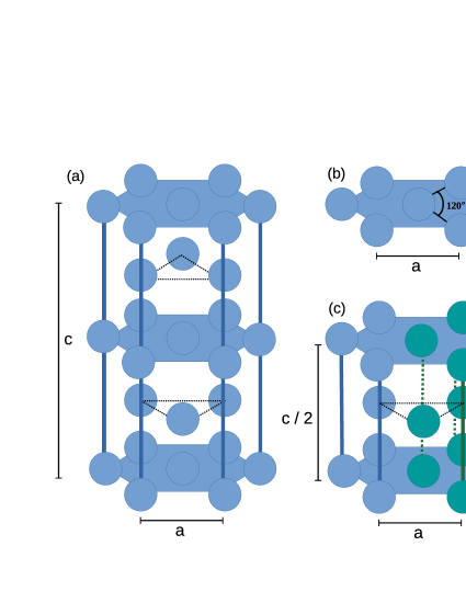
Figure 1: (Color online)(a) Double hexagonal closed packed dhcp structure. In, (b) the primitive vectors and (c) the primitive cell of the dhcp lattice containing 4 atoms (in green).

$$dhcp-La=\left\{\begin{array}[]{ll}\vec{a}_{1}=\frac{a}{2}n_{x}\hat{x}-\frac{\sqrt{3}a}{2}n_{y}\hat{y}\\ \vec{a}_{2}=\frac{a}{2}n_{x}\hat{x}+\frac{\sqrt{3}a}{2}n_{y}\hat{y}\\ \vec{a}_{3}=cn_{z}\hat{z}\end{array}\right.$$ (57)

After convergence test, the resulting lattice parameters ($a,c$ and $c/a$) and the volume of La ion ($\Omega^{I}$) are respectively, $a=3.774$ Å, $c=12.084$ Å, $c/a=3.202$ or $c/2a=1.601$, $\Omega=37.15$ ų   and the formation energy per atom ($E_{0}$) $E_{0}=-4.90$ eV/atom. Table 1 summarizes the optimized structure of dhcp-La.

The minimum Energy per atom, $E_{0}$, and respective volume were obtained from a parabolic fit using a 3^rd order Birch-Murnaghan equation. This results are shown in Figs. 2 for both, the GGA(Left) and GGA+U(Right) approximations.

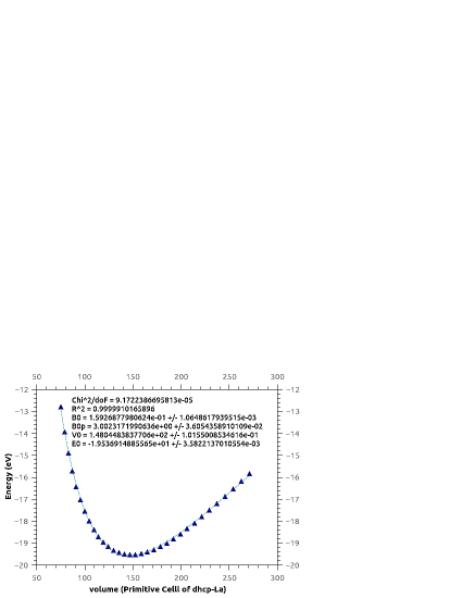
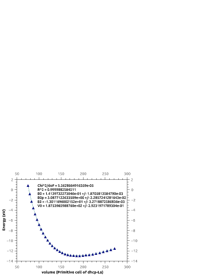
Figure 2: Birch-Murnaghan 3^rd order equation of states fitting to the calculated E-V data of dhcp-La from (Left) GGA and (Right) GGA+U($U=5$eV) calculations with VASP.

Table 1: Optimized dhcp La lattice parameters, $c/a$ and $a$. The corresponding ion volume $\Omega$ and the relative total energies $E_{0}$ per atom.

Host	$c/a$	$a$(Å)	$E_{0}$(eV)	$\Omega$(Å)3
La4	3.202	3.774	-4.89	37.15
La4(GGA+U)	3.225	3.770	-4.71	37.41
Ref.[18]	3.206	3.754		36.71
Ref.[19]	3.225	3.774
La16	3.206	3.777	-4.89	37.18
La36	3.208	3.776	-4.89	37.18

As shown in Table1 our results are in well agreement with the calculated values of $c/a=3.206$; $a=3.754$ and $\Omega=36.71$ by Schöllhammer et al. in Ref. [18] and with the experimental data of $c/a=3.225$ for $a=3.774$ in Ref.[19].

Concerning to the electronic properties of the dhcp Lanthanum, Table 2 summarizes (in eV) the Fermi energy, $E_{f}$, the energy center of s- and d- bands, $\epsilon^{s,d}_{c}$, and the bandwidth of the, $\Delta_{s,d}$.

Since the expression of the resistivity, $R$, in (1) depends on the Fermi level and the energy of the center of the d-band, Table 2 also shows both, the calculated values of the Fermi energy, $\epsilon_{F}$, and the energy of the center of the $s,d$-bands, $\epsilon_{c}^{s,d}$, the last also obtained with the Vaspkit utils [15] from present calculations of the density of states of La.

Table 2: The Fermi energy (in eV), $E_{f}$, The center of the s,d-bands, $\epsilon^{s,d}_{c}$, in the energy range of [-5,15]eV referenced to $\epsilon_{F}=0$ eV, and the bandwidth $\Delta_{s,d}$ for Lanthanum.

T	$\epsilon_{F}$	$\epsilon^{s}_{c}$	$\epsilon^{d}_{c}$	$\Delta_{s}$	$\Delta_{d}$
La4	7.83	6.35	4.62	17.29	17.12
La4 GGA+U	8.19	6.04	5.34	17.59	17.54

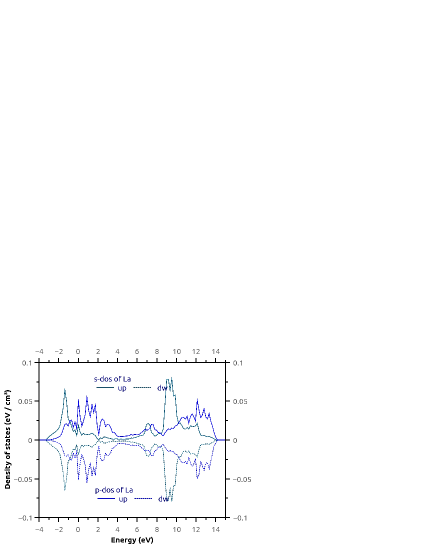
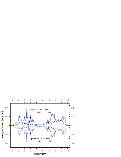
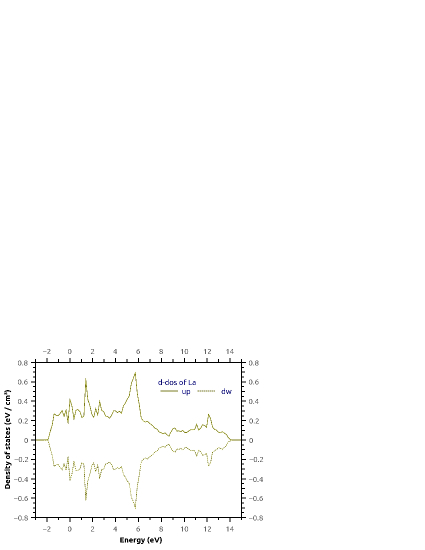
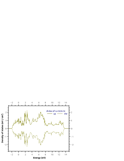
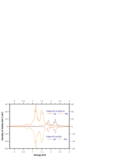
Figure 3: Density of states of the primitive cell of lanthanum (in eV/cm³) vis Energy (in eV).

In Figure 3 we present DFT results of the DOS

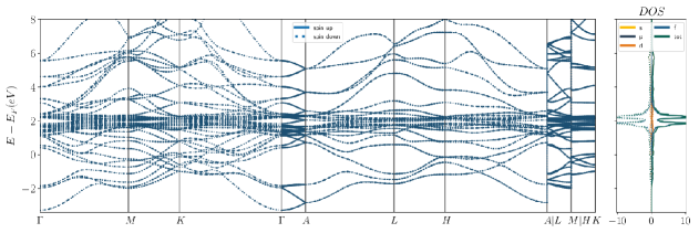
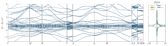
Figure 4: Band structure and density of states of La (Above: GGA) and (Below: GGA+U; U=5).

Our band structure of La is in agreement with the results in Ref.[20]. We also present our results of the density of states and the band structure of the lanthanum supercell $La_{16}$ containing 16 atoms from which we built the alloy by including one sustitutional atom of impurity. Fig.5 shows the band structure of the Lanthanum supercell. Table 4 summarizes the impurity-host charge difference, $\Delta Z=Z_{I}-Z_{h}$, the volume differences between impurity and host elements, $\delta v/\Omega$ in (56) and the energy difference $\Delta E$ between the pure host and the host containing one sustitutional solute atom.

Figure 5 shows the band structure (Left) and the density of states (Right) of the supercell containing 16 lanthanum atoms. From this supercell we built the alloys studied containing 15 La atoms and one impurity atom placed at a substitutional site within of $La_{16}$ supercell. From this resdults, we will then compare the differences observed in the densities of states and the band structure of pure metal with those corresponding to the alloys.

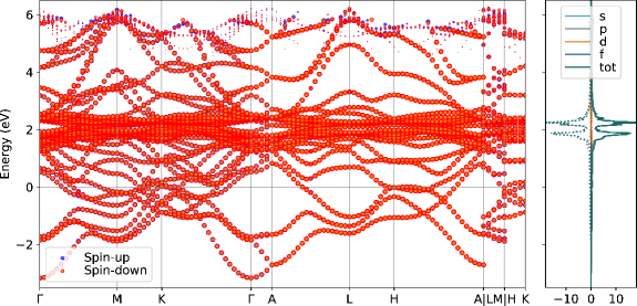
Figure 5: Density of states and band structure for the Lanthanum supercell containing 16 atoms.

Present calculations of the critical potential, $V_{dd}^{c}$ (in eV), for the “parabolic” model in eq.(58) and DFT calculations for each atomic specie of the 5-d serie hosts. $V_{sd}$ obtained as the limit of validity of the approximation $|V_{sd}|^{2}\theta(\epsilon_{F})$.

Here, calculations of the resistivity, $R$, using the realisic the density of states model for La, assume that the center of the s-band, $\varepsilon^{s}_{c}$, the d-band, $\epsilon^{d}_{c}$, and the energy of the Fermi level, $\epsilon_{F}$ are different of zero as in the case of the parabolic model (i.e., $\varepsilon^{s}_{c}=\epsilon^{d}_{c}=\epsilon_{F}=0$). Our results are shown in Table 2. In Tables 3 and 4, show the characteristics parameters of interest in this work, taken from Ref. [21].

For rare earths impurities, the exchange interactions are usually described using an indirect exchange mechanism [29]. The $4f$ spin of the rare earth induces a positive local $5d$ spin moment through the ordinary intra-atomic $4f-5d$ exchange interactions. In fact, because of the localized nature of the $4f$ electronic shell, the interaction between the $4f$ spin and an itinerant electron spin can occur only through the local exchange interaction on the rare-earth atom, described by the intra-atomic exchange integrals $J_{4f-5d}$, $J_{4f-6s}$ and $J_{4f-6p}$, where among these three exchange integrals, the first one, $J_{4f-5d}$, is dominant [29]. Then, we use the exchange integrals $J_{4f-6s}$, $J_{4f-6p}$ and $J_{4f-5d}$ from relativistic atomic calculations for most of the rare-earth elements calculated in Ref.[30] which are summarized in Table 3. From Table 3 we obtain the needed ratios $J^{(d)}/J^{(s)}=5$ and $J^{(s)}/J^{(d)}=2$ that appear in equation (3). As, $J^{(s)}$ and $J^{(d)}$ are normalized by the s- and d- bandwidths, $\Delta_{s,d}$, in our model and furthermore, from our DFT results, the ratios $\Delta_{s}/\Delta_{d}$ and $\Delta_{d}/\Delta_{s}$ are approximately 1, so we assume $J^{(d)}/J^{(s)}=5$ and $J^{(s)}/J^{(d)}=2$ in all the present resistivity calculations for both, the parabolic and DFT models that we have assumed for the band structure of Lanthanum.

Experimental results of the resistivity of fcc and hcp $La$ containing small amounts (from 0.5 up to 3%) of rare earth (RE) impurity as Gd are taken from Ref.[25]. Also the effective $s-f$ exchange integral for $J_{eff}^{(s)}$ has been calculated from the resistivity data. In [25] the authors have compared $J_{eff}^{(s)}$ with the values calculated from the change of the superconducting transition temperature $\Delta T_{c}$ by Abrikosov and Gor’kov [26] as, $\Delta T_{c}=T_{c}(La-1\%Re)-T_{c}(La)$, the critical tempeature $Tc$ for the fcc La-RE alloys containng 1%at RE and the pure $T_{c}$ of fcc La. In our model, we have neglected the term $H^{Imp}_{Coul.}=\Delta Un^{(d)}_{0\uparrow}n^{(d)}_{0\downarrow}$ with $\Delta U=U_{imp}-U_{host}$, being $U$ the Coulomb repulsion parameter at the impurity site [28].

The values obtained in Ref. [25] are $J_{eff}(La-1\%Gd)=0.047$ eV, $J_{eff}(La-1\%Tb)=0.066$ eV and $J_{eff}(La-0.93\%Dy)=0.087$ eV. The magnitude and sign of $J_{eff}$ or RE diluted in metals depends on the degree of mixing of the $4f$ electrons with conduction electrons and also on the conduction band nature of the host. Since in La and Y the dependense of the mixing of the solute $4f$-electrons with the conduction electrons are similar. Alternative values for the exchange parameters could be $J_{eff}(Y-1\%Gd)=0.047$ eV, $J_{eff}(Y-1\%Tb)=0.066$ eV and $J_{eff}(Y-0.93\%Dy)=0.087$ eV.

In Table 3, the values of a magnetic exchange coupling $J_{f-d}$ in meV of the Gd³⁺, Dy³⁺ and Tb³⁺ 4f electrons couple with the 5d conduction electrons of the host. For instance, for Gd₃, Tb₃ and Dy₃ strongly localized, semi-core $f$ electrons are treated as core states despite being higher in energy than other valence states. The Gd³⁺ $4f$ electrons couple with the $5d$ conduction electrons with a magnetic exchange coupling is also presented in the same Table.

Table 3: The impurity exchange parameters (in eV).

Impurity	$J_{4f-5d}$	$J_{4f-6s}$	$J_{4f-6p}$
Gd3+	0.1891	0.0377	0.0151
Tb3+	0.1837	0.0375	0.0148
Dy3+	0.1797	0.0374	0.0145

Then, the conduction electrons are coupled to the impurity spin $\vec{S}_{0}$ expected to be $S_{0}(Gd)=7/2$ while for impurities as $Tb$ and $Dy$, with $L\neq 0$, we replace $S_{0}$ in (50) by $(g_{j}-1)J_{0}=S_{0}^{eff}$, being $(g_{j}-1)$ the De Gennes factor, is the projection of the spin $S_{0}$ on the total angular momentum $J_{0}$ of the $Tb$ or $Dy$ impurities. So, $S^{eff}_{0}(Tb)=6/2$ and $S^{eff}_{0}(Dy)=5/2$. The values of $J_{f-s}$ and $J_{f-d}$ employed in present calculations of the temperature resistivity are summarized in Table 3. In Table 4, $g_{L}$ is the Landé factor and $J$ is the total moment for the Gd and $g_{L}J$ is the contribution due to 5d conduction electrons.

Table 4: Some characteristics of Gd, Tb, Dy and Lu taken from Ref.[21]

Imp.	Elec. Config.	$g_{L}$	$J$	$g_{L}J$
Gd	$[Xe]4f^{7}5d^{1}6s^{2}$	2	7/2	7
Tb	$[Xe]6s^{2}4f^{9}$	3/2	6	9
Dy	$[Xe]4f^{10}6s^{2}$	4/3	15/2	10
Lu	$[Xe]4f^{14}5d^{1}6s^{2}$	0	0	0

The impurity valence states $4f^{7}5d^{1}6s^{2}$ for Gd (in the atomic configuration) is $4f^{n-\delta}5d^{m+\delta}6s^{2}$, where $\delta$ is the amount of charge transferred from the 4f-resonance to the d-conduction band. Since the Gd valence state lies in the interval [3.2-3.4] we have self-consistently obtained $\delta=0.125$. Total-energy calculations of the diluted rare-earth impurity $I$ in Lanthanum based on density-functional theory (DFT), allowed us to estimate the strength of the energy difference between the alloy and the host.

Although for Gd, with a pure spin moment of $J\equiv S=7/2$, the paramagnetic susceptibility is isotropic, i.e., for pure spin magnetism there is no crystal field interaction, this is different for the other RE metals that have a finite orbital moment, $L$. As is the case of $Tb$ and $Dy$ impurities, with $L\neq 0$, one can consider also by substituting $S_{0}$ by $(g_{j}-1)J_{0}=S_{0}^{eff}$, with $(g_{j}-1)$ called the De-Gennes factor, is the projection of the spin $S_{0}$ on the total angular momentum $J_{0}$ of the $Tb$ or $Dy$ impurities. So, $S_{0}(Gd)=7/2$, $S^{eff}_{0}(Tb)=6/2$ and $S^{eff}_{0}(Dy)=5/2$. Where, $S_{0}$ and $S^{eff}_{0}$ are good quantum numbers and they arise from Hund’s rules. In Table 5 we show our DFT calculations of the impurity-host charge difference, $\Delta Z=Z_{I}-Z_{h}$, calculated as the difference between the occupation numbers, $<n_{s,d}>$ (with $<n_{d}>=0.1768$ La), of the host and the impurity, the volume difference introduced by impurity $\delta v/\Omega$ (56) and the energy difference $\Delta E=E(La-I)-E(La)$ (with I=Gd, Tb, Dy and Lu), being $E(La-I)$ the energy of La containing one impurity atom, and the host and $E(La)$ the energy of La.

Table 5: The impurity-host charge difference, $\Delta Z=Z_{I}-Z_{h}$, the ocupation and volume difference $\Delta<n>$, $\delta v/\Omega$ between impurity and La-host; and the energy difference $\Delta E$ between the pure host and the alloy.

Metal-host				Gd3+	Tb3+	Dy3+	Lu3+
T	Elec. Config.	Struct.	$v_{ion}$ (Å3)	$\delta v/\Omega$	$\delta v/\Omega$	$\delta v/\Omega$	$\delta v/\Omega$
La	$[Xe]5d^{1}6s^{2}$	dhcp	37.15	-0.1282	-0.1395	-0.1419	-0.2106
			$\Delta E$	-0.28	-0.30	-0.34	-0.42
			$\Delta Z$	-0.889	-0.788	-0.688	-0.770

In Fig.3 we show our results of the calculated DOS using the GGA (Left) and GGA+U (Right) approximations for the exchange and correlation parametrization term. In both cases the DOS of the s- and p-bands are shown together while for the d-band these are presented separately. At the bottom, we show our results for the f-band of both, the GGA and GGA+U calculations. We observe a notory density of states shape difference with GGA and GGA+U calculations, although this DOS shape difference has not been reflected in the results of the calculated resistivity, as we show below. In regarding the band structure, we have also observed some differences between both calculations. However, the conclusions about the calculated resistivity values will be shown in a future work, because these calculations are beyond the scope of this work. We intend to calculate the electrical conductivity of the systems we study here using the Python module, BoltzTrap2, which uses the band structure calculations obtained in this work and presented in Fig.4. The Boltztrap2 module calculates the conductivity based on the semiclassical Boltzmann theory of the electronic transport [22]. The role of the band structure in resonant scattering (virtual bound states) is discussed here adopting a realistic band structure and a “parabolic” model of the DOS to establish a comparison of our results for the resistivity. In this way, and to bring out the effects due to the changes of $d$-band shape in transition metals, we have used a ” parabolic” density of states model chosen as,

$$\rho_{\lambda}(\epsilon)=\alpha_{\lambda}(\epsilon^{2}-\Delta^{2}_{\lambda})\,\,\,\mathrm{(\lambda=s\,or\,d)},$$ (58)

where the $\alpha_{\lambda}$ are normalization constants, which are taken as $0.75\Delta^{-1}_{\lambda}$, in order to give one electron per atom (degeneracy is included in the above formulas) and $\Delta_{\lambda}$.

The value of $\Delta_{\lambda}$, is estimated from band calculations (e.g. $\Delta_{d}/\Delta_{s}$ as 0.88, for dhcp La. $\rho_{\lambda}(\epsilon)$ in (58) is used to simulate for band fillings of $n_{e^{-}}=5$.

From the values of the $d$-band DOS, $\rho_{d}$, the Fermi energy $\epsilon_{F}$, the $s,d$-band center, $\epsilon_{c}^{s,d}$ in Table 2, and the critical potential $V_{dd}^{\star}$ in equation (41), we calculate the repulsive critical potential from $\eta_{dd}$ (see Appendix A eqn.(70)) as,

$$\eta_{dd}(\epsilon)=\cos^{-1}\frac{1-|V_{dd}^{\star}(\epsilon)|F_{d}^{R}(\epsilon)}{[1-V_{dd}^{\star}(\epsilon)F_{d}^{R}(\epsilon)]^{2}+[V_{dd}^{\star}(\epsilon)F_{d}^{I}(\epsilon)]^{2}}\,.$$ (59)

The limiting value of $V_{dd}$ is obtained by changing the position of the Fermi level in the band structure in order to scan the neighborhood of the top of the band. Numerically, the existence of bound states is determined by a critical value of $V_{dd}$, calculated as $V^{c}_{dd}=\left[F^{R}_{d}(E_{top})\right]^{-1}$, with $E_{top}$ the energy of the top of the d-band. The calculated critical potencial, $V_{dd}^{c}$, as a function of $|V_{sd}|^{2}/\Delta_{s}$ is presented for the “parabolic” model and for DFT in Figs. 6 and 7, respectively. Also in the same figures Solid and dotted lines corresponds respectively to $\alpha\neq 1;\delta v/\Omega\neq 0$ (LaI) and $\alpha=1;\delta v/\Omega=0$ (LaI2) for the La containing one Impurity (I) atom.

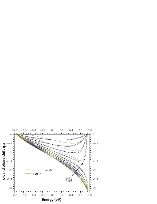
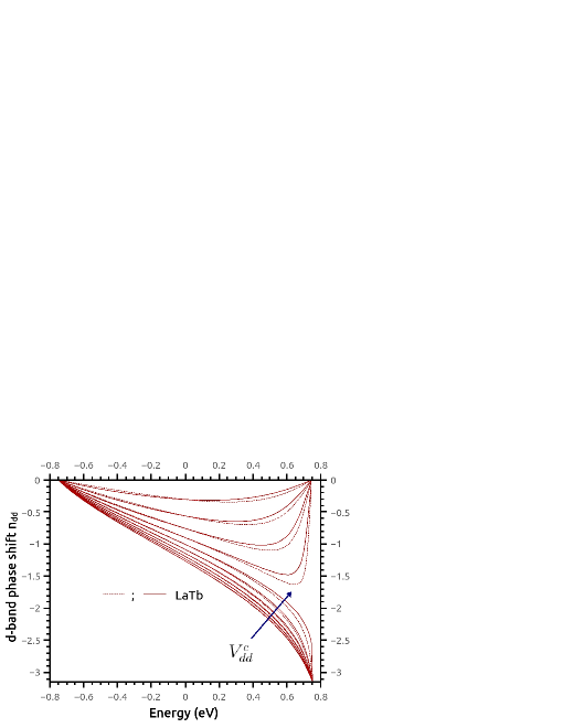
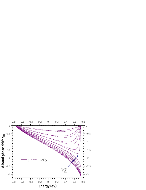
Figure 6: Phase shift $\eta_{dd}$ computed using the DFT band model for several self-consistent values of the $V_{dd}$. Critical potential $V_{dd}^{c}=0.683$ eV with a parabolic band $\rho_{\lambda}(\omega)=\alpha_{\lambda}(\omega^{2}-\Delta^{2}_{\lambda})$ ($\lambda$ = s,d). Solid lines $\alpha\neq 1$; $\delta v/\Omega\neq 0$ and dotted lines $\alpha=1$; $\delta v/\Omega=0$ in eqs. (41) and (56).

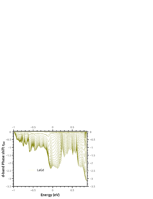
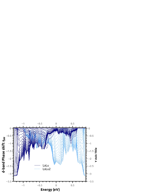
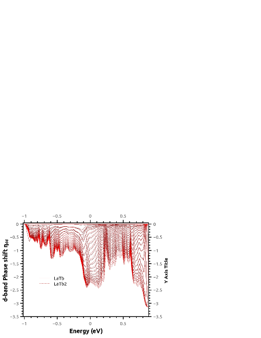
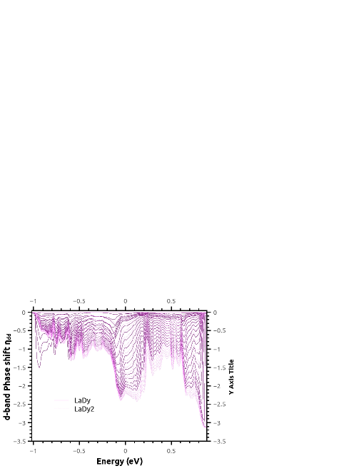
Figure 7: Phase shift $\eta_{dd}$ computed using the DFT band model for several self-consistent values of the $V_{dd}$. Solid lines $\alpha\neq 1$; $\delta v/\Omega\neq 0$ and dotted lines $\alpha=1$; $\delta v/\Omega=0$ in eqs. (41) and (56).

In Figs.6 and 7, $V_{dd}$ goes from $V_{dd}=0.05$ eV up to $V_{dd}^{+\infty}=3.0$ eV. Also they show the critical value $V_{dd}^{c}$ for La in the alloy using the “parabolic” DOS model in eq.(58) and the calculated DOS model with VASP, respectively. With the “parabolic” model the critical value occurs at $V_{dd}=0.683$ for all the cases; While in DFT the behavior of $\eta_{dd}$ is considerably different. In 6 there is a clear discontinuity in $\eta_{dd}$ at $V_{dd}^{c}$, value from which the existence of bound states is determined which have not been observed in the case of DFT for the same energy range. In Figs.6 and 7, solid lines correspond to the case when the period, $\alpha\neq 1$, and volume effects, $\delta v\neq 0$, are considered; while dotted lines correspond to the cases where the period, $\alpha=1$, and volume effects, $\delta v=0$ are not considered in agreement with the theoretical results of Troper and Gomes in Ref. [1].

In a future work, we intend to calculate the electrical conductivity of the systems we study here using the Python module, BoltzTrap2, which uses the band structure calculations obtained in this work and presented in Fig.4. The Boltztrap2 module calculates the conductivity based on the semiclassical Boltzmann theory of the electronic transport [22]. In this way, we can submit our theoretical predictions to experimental check when experimental data exist, otherwise we compare with calculated resistivities using BoltzTraP module which uses our results of the Band structure calculations with VASP.

In Figs. 8 to 11 we present respectively, our results obtained with VASP of the density of states and the band structures of the dilute La alloys containing a substitutional atom of rare earth impurities of Gd, Tb, Dy and Lu that make up the four alloys studied in this work. Although neither the DOS nor the band structures (BS) of the alloys will be used in this work, we have advanced our results here to see if there are important differences with the case of pure Lanthanum.

Present results of $\Omega$ (in ų ) calculated with VASP, are in very well agreement with the results in Refs. [17] and [21]. Our $\delta V/\Omega$ values from DFT results are in well agreement with those obtained in Ref.[23]. Since the resistivity depends on the Fermi level and the energy of the center of the $s,d$-bands, Table 2 also shows both, the calculated values of the Fermi energy, $\epsilon_{F}$, and the energy of the center of the s,d-bands, $\epsilon_{c}^{s,d}$, the last also obtained with the Vaspkit utils [15] from the density of states calculations.

We show the DOS of the Gd, Dy, Tb and Lu diluted in dhcp-La, namely: La₁₅Gd, La₁₅Gd, La₁₅Gd and La₁₅Gd. Calculations were performed for a supercell of 16 atoms constructed from the coordinates of the primitive cell of La₄ using vaspkit [15] with $n_{x}=n_{y}=2$ and $n_{z}=1$. In the alloy de impurities are included at sustitutional sites; and the density of states and the band structure were calculated as follows: After relaxation of the supercell containing one impurity atom I, La₁₅I, we relax only on the atomic position while the size and the volume of the supercell are kept fixed. For DOS calculations we duplicate de quantity of k-points with respect to the bulk relaxation. While, the high simmetry k-points of the alloy were obtained for UNFOLDING calculations using the VASP vaspkit util which we later checked on the seek site [16].

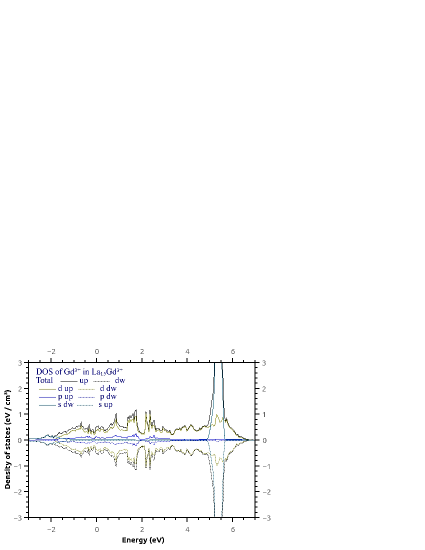
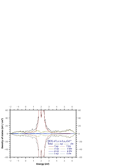
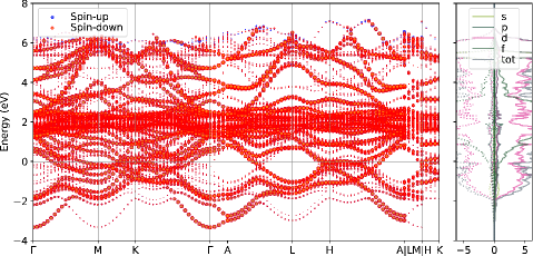
Figure 8: Density of states (in eV/cm³) vis Energy (in eV) of La₁₅Gd. For La and Gd we show (Left) the s,p bands and (Right) d-band.

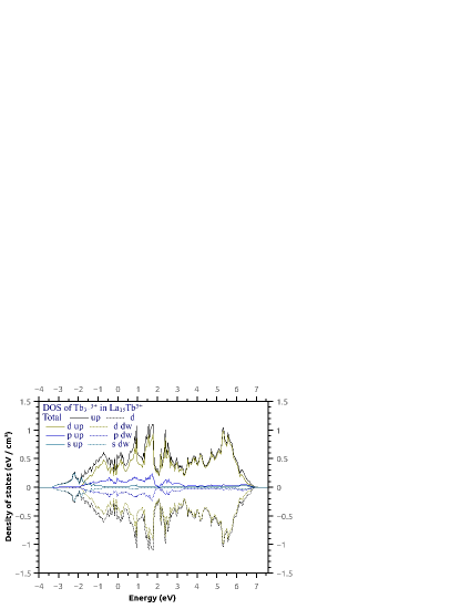
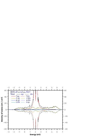
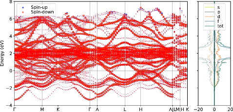
Figure 9: Density of states (in eV/cm³) vis Energy (in eV) of La${}_{1}5$Tb. For La and Tb we show (Left) the s,p bands and (Right) d-band.

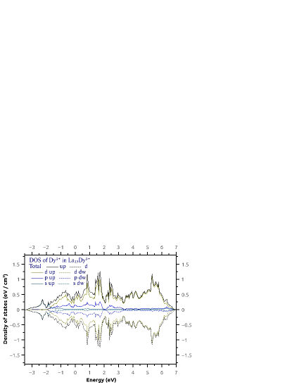
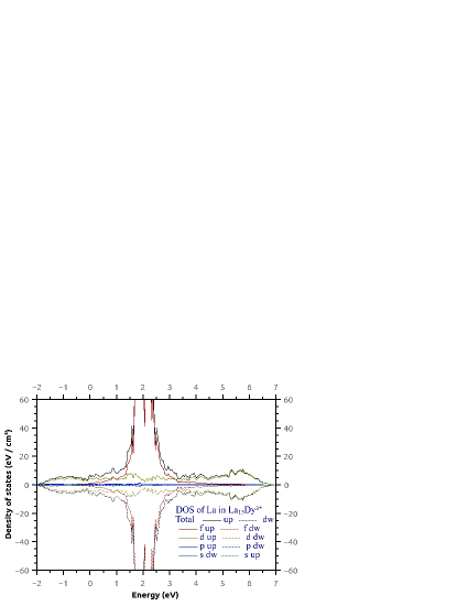
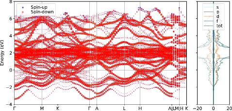
Figure 10: Density of states (in eV/cm³) vis Energy (in eV) of La${}_{1}5$Dy. For La and Dy we show (Left) the s,p bands and (Right) d-band.

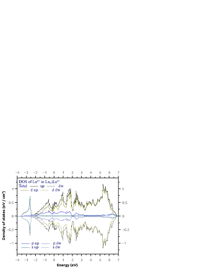
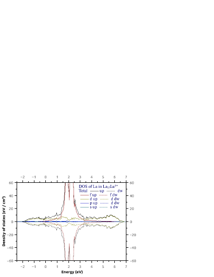
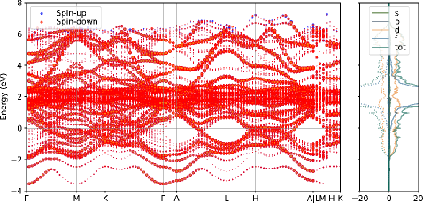
Figure 11: Density of states (in eV/cm³) vis Energy (in eV) of La${}_{1}5$Lu. For La and Lu we show (Left) the s,p bands and (Right) d-band.

Finally, we present our results of the temperarure independent resistivity, $R$, in (1). First, we have calculated all the magnitudes involved in $R_{0}$ (51) and $\theta$ (3) as, the density of states and the bandwdiths of the $s,d$-bands, also the energy of the Fermi level, $\epsilon_{F}$ are required to compute each term in $R$. The $V_{dd}$ scattering matrix element is obtained via an extended Friedel’s sume rule (see Appendix B).

In Figs. 12 and 13; and Figs. 14 and 15 we present our results of the resistivity respectively calculated with the “parabolic” band model in (58) and from DFT calculations with VASP. In these figures, Solid/dotted lines respectively for the cases $\alpha\neq 1$; $\delta v/\Omega\neq 1$ which represents the extended and improved model of that in Ref.[1] where the authors assumed $\alpha=1$; $\delta v/\Omega=1$ in their model.

In Figs12 we present the Resistivity of Gd, Dy, Tb and Lu diluted in La vis $|V_{sd}/\Delta_{s}|$ using the “parabolic” band model. For the LaGd solo mostramos los resultados cuando concideramos los efectos de periodo, $\alpha\neq 1$, y de volumen $\delta v\neq 0$ mientras que el caso $\alpha=1$ y $\delta v=0$, no converge. Notamos que el termino efectivo de De Gennes y Friedel $R_{DG-F}^{eff}$ puede tomar valores tanto positivos como negativos, que tienen una influencia considerable en el valor de $R$ total. Este comportamiento se observa en los casos $LaGd$, $LaTb$ y $LaDy$. En el caso del $LaLu$ no hay contribución de spin a la resistividad. En la Figura 13 presentamos cada término en $R$, i.e. $R_{0}$, $R_{DG-F}^{eff}$ and $R$, separadamente.

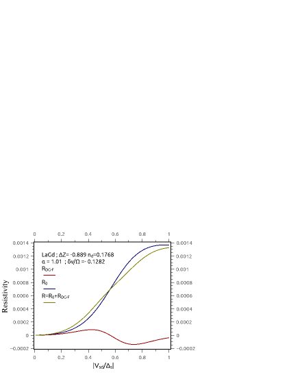
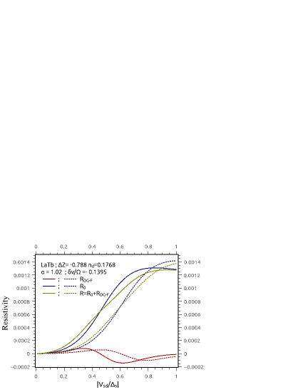
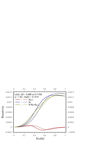
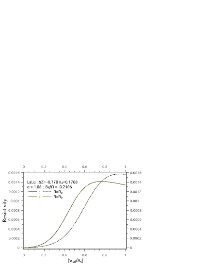
Figure 12: Resistivity of Gd, Dy, Tb and Lu in La vs $|V_{sd}/\Delta_{s}|$ (“parabolic” band).

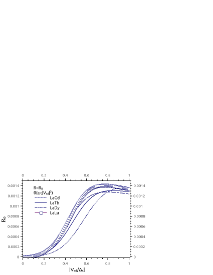
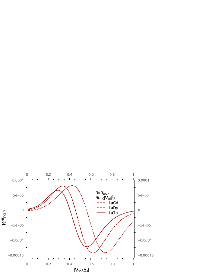
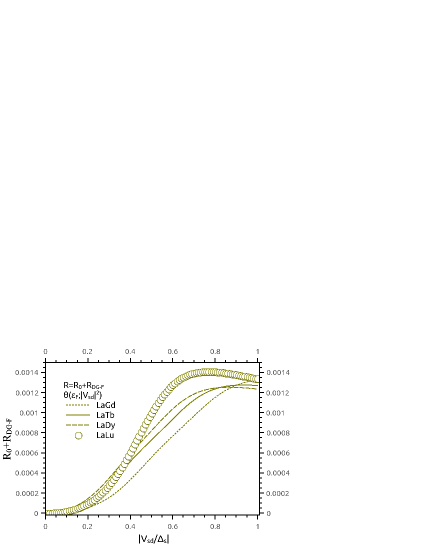
Figure 13: Comparison of Resistivity of Gd, Dy, Tb and Lu in La vs $|V_{sd}/\Delta_{s}|$ (“parabolic” band).

En las Figuras 14 y 15 we present the Resistivity of Gd, Dy, Tb and Lu diluted in La vis $|V_{sd}/\Delta_{s}|$ using the DFT band model. Again, in these figures, Solid/dotted lines respectively for the cases $\alpha\neq 1$; $\delta v/\Omega\neq 1$ and $\alpha=1$; $\delta v/\Omega=1$, respectively. For this case substantial differences were observed with respect to the “parabolic” model. Here the behavior of the resistivity changes drasticaly from XXX to a parabolic behavior in terms of the scatterig matrix element $V_{sd}$. The effective De Gennes - Friedel resistivity, $R_{DG-F}^{eff}$, takes positive values in the same $|V_{sd}|$ range than the assumed in the previous case.

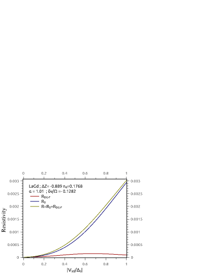
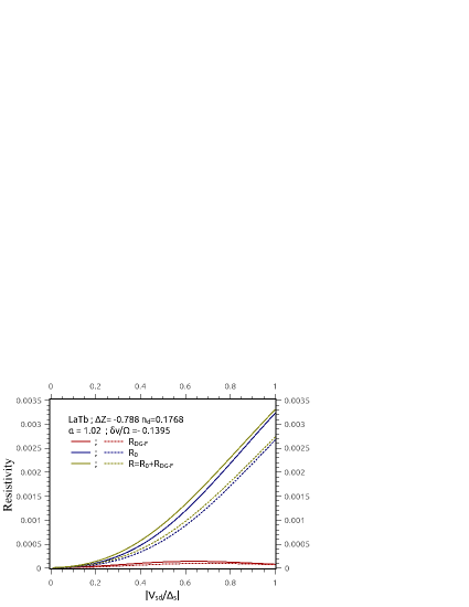
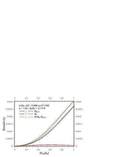
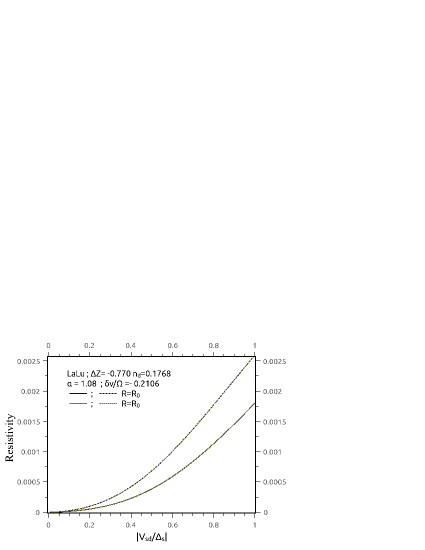
Figure 14: Resistivity of Gd, Dy, Tb and Lu in La vs $|V_{sd}/\Delta_{s}|$ (DFT band model).

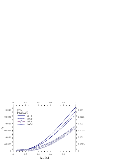
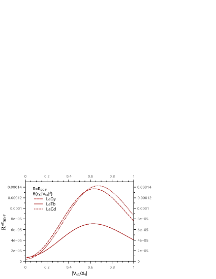
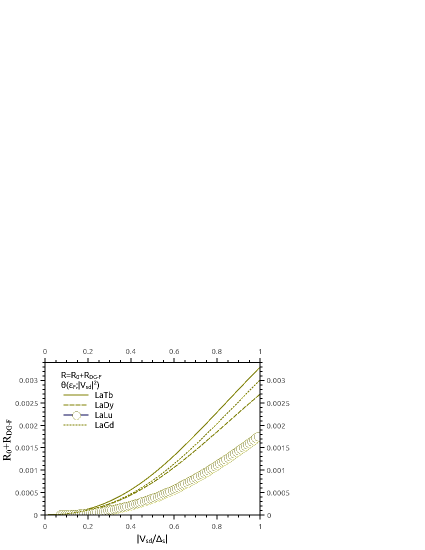
Figure 15: Comparison of Resistivity of Gd, Dy, Tb and Lu in La vs $|V_{sd}/\Delta_{s}|$ (DFT band model).

Figures 16 and 17 show present results of Resistivity for the exact, $\theta(\epsilon_{F},|V_{sd}|^{2})$, and approximate, $|V_{sd}|^{2}\theta(\epsilon_{F})$, expressions of $R=R_{0}+R_{DG-F}^{eff}$ in (51) and (52) respectively for the “parabolic” band model and from a realistic one from VASP calculations.

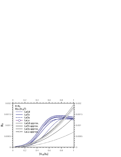
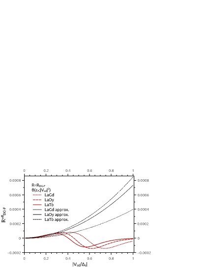
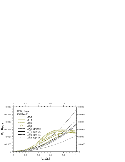
Figure 16: Comparison of exact y approximate results of Resistivity of Gd, Dy, Tb and Lu in La vs $|V_{sd}/\Delta_{s}|$ (“parabolic” band) for $\delta v/\Omega\neq 0$ and $\alpha\neq 1$.

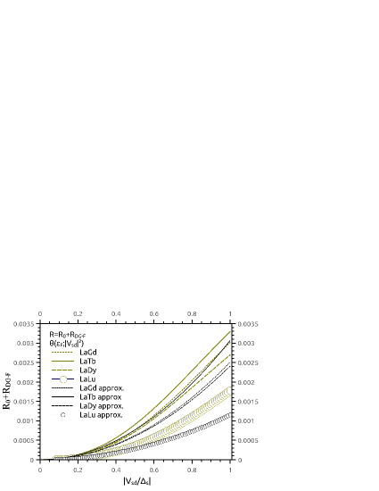
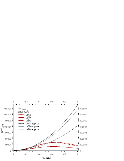
Figure 17: Comparison of exact y approximate results of Resistivity of Gd, Dy, Tb and Lu in La vs $|V_{sd}/\Delta_{s}|$ (DFT band model) for $\delta v/\Omega\neq 0$ and $\alpha\neq 1$.

6 Comments and conclusion

In brief, we study the dependence of the temperature-independent resistivity on the band structure of the 5d-serie Host. We start from the case of diluted Lanthanum alloys containing rare earth impurities such as Gd, Tb, Dy and Lu. With this purpose, we use two types of models for the band structure, one known as a “parabolic” type band and another more realistic one derived from first-principles calculations using the VASP code. Our results have corroborated the strong dependence of the band structure on the Resistivity and therefore on the shape of the DOS used. As evidence of this conclusion, we have observed that:

1. Our expression of the temperature independent resistivity in terms of the hybridization charge potential, $|V_{sd}|^{2}$, changes drastically if we use the parabolic or the realistic model for the DOS.

2. Also, we study the exact form of the resistivity, $R_{e}=R(\epsilon,|V_{sd}|^{2})$, and the approximate case, $R_{a}=|V_{sd}|^{2}R(\epsilon)$, up to first order in $|V_{sd}|^{2}$. We notice that, with the DOS-Moriya the interval of $|V_{sd}|^{2}$ values in which $R_{e}\simeq R_{a}$ is smaller than for the realistic DOS. While, for the last case, the $R_{a}$ is practicaly equal in the whole interval of $V_{sd}$ considered.

3. As per we have observed in 2., for the case of the realistic DOS we have the possibility of separating the s-d charge effects from the d-d ones assuming the approximation up to first order in $|V_{sd}|^{2}$. These results will be presented in a next work.

4. Given the important consequences of the DOS on the temperature independent of the temperature, $R$, we have performed the systematic for transition metal hosts belong the 5d series as: Hf, Ta, W, Re, Ir, Os, Pt and Au. These results will be also presented in a future work.

5. In the case of the transition-metals, the expression of the resistivity has the exchange parameters appearing as $(J^{(s)})^{2}$, $(J^{(d)})^{2}$ and $J^{(s)}\times J^{(d)}$. Here, we have demonstrated that, these cross products strongly affect the magnitude of the derived $J^{(s)}_{eff}$ in (52).

6. The existence of two bands (s and d) and consequently, two exchange couplings, may change the standard result of De Gennes and Friedel [10].
   From our model is clear that the rare-earth impurity introduced in the transition host acts in two ways:

7. The simplest effect is that the f level (supposed to lie below the conduction s-d bands) provides only a source of one-electron spin-dependent potential via the exchange interactions $J^{(s)}$ and $J^{(d)}$.

8. The valence state of the usual rare earths (trivalent in general) introduces a source of scattering. In the case discussed here, primary importance is given to the nature of the host, namely, the existence of $s-d$ bands.

9. The best way to discuss the role of the band structure in resonant scattering (virtual bound states) is to adopt a realistic band structure as performed in present calculations.

In a future work, we also include the electronic transport calculations using VASP as implemented in the semiclassical python module BoltzTrap2, which uses our present results of the Band structure calculations with VASP. In this way we compare our numerical results with those obtained with VASP+BoltzTrap2 when there are not available experimental data.

Appendix A Phase shift parameters

Taking into account the following definition

$$F_{\lambda}(\epsilon\pm i\delta)=F_{\lambda}^{R}(\epsilon)\mp F_{\lambda}^{I}(\epsilon),$$ (60)

with $F_{\lambda}^{R}$ the real part of $F$

$$F_{\lambda}^{R}(\epsilon)=P\sum_{k}\frac{1}{\epsilon-\epsilon_{k}^{(\lambda)}}=P^{\lambda}_{00},$$ (61)

and the imaginary part as

$$F_{\lambda}^{I}(\epsilon)=\pi\rho_{\lambda}(\epsilon),$$ (62)

with $\rho_{\lambda}(\epsilon)$ the density of states of the conduction electrons. Introducing the expressions for the phase-shift , we write

$$F_{\lambda}(\epsilon\pm i\delta)=|F_{\lambda}(\epsilon)|e^{\mp i\delta(\epsilon)},$$ (63)

where

$$|F_{\lambda}(\epsilon)|=\left\{[F_{\lambda}^{R}(\epsilon)]^{2}+[F_{\lambda}^{I}(\epsilon)]^{2}\right\}^{1/2},$$ (64)

with

$$\cos\delta_{\lambda}(\epsilon)=\frac{F_{\lambda}^{R}(\epsilon)}{|F_{\lambda}(\epsilon)|},$$ (65)

and

$$\mbox{sen}\delta_{\lambda}(\epsilon)=\frac{F_{\lambda}^{I}(\epsilon)}{|F_{\lambda}(\epsilon)|}.$$ (66)

$$F_{s}(\epsilon\pm i\delta_{s})F_{d}(\epsilon\pm i\delta_{d})=|F_{s}(\epsilon)||F_{d}(\epsilon)|e^{\mp[\delta_{s}+\delta_{d}]}.$$ (67)

Similarly,

$$1-V_{dd}(\epsilon)F_{d}(\epsilon)=|1-V_{dd}(\epsilon)F_{d}(\epsilon)|e^{\mp i\eta_{dd}(\epsilon)},$$ (68)

where

$$|K(\epsilon)|=1-V_{dd}(\epsilon)F_{d}(\epsilon)=\left\{[1-V_{dd}(\epsilon)F_{d}^{R}(\epsilon)]^{2}+[V_{dd}(\epsilon)F_{d}^{I}(\epsilon)]^{2}\right\}^{1/2}.$$ (69)

Again, we define the functions:

$$\cos\left[\eta_{dd}(\epsilon)\right] = \frac{1-V_{dd}(\epsilon)F_{d}^{R}(\epsilon)}{|K(\epsilon)|},$$ (70)

$$\mbox{sen}\left[\eta_{dd}(\epsilon)\right] = -\frac{V_{dd}(\epsilon)F_{d}^{I}(\epsilon)}{|K(\epsilon)|}$$ (71)

In the following we present some expressions obtained in Ref.[1] with the idea to show how these expressions are modified when we assume the approximation studied in the present work.

$$1-V_{dd}(\epsilon)F_{d}(\epsilon)-|V_{sd}|^{2}F_{s}(\epsilon)F_{d}(\epsilon)=|K(\epsilon)|e^{\mp i\eta(\epsilon)},$$ (72)

where

$$|K(\epsilon)| = \left\{\left[1-V_{dd}(\epsilon)F_{d}^{R}(\epsilon)-|V_{sd}|^{2}[F_{d}^{R}(\epsilon)F_{s}^{R}(\epsilon)-F_{d}^{I}(\epsilon)F_{s}^{I}(\epsilon)]\right]^{2}\right.$$ (73)

$$+ \left.\left[-V_{dd}(\epsilon)F_{d}^{I}(\epsilon)-|V_{sd}|^{2}[F_{d}^{R}(\epsilon)F_{s}^{I}(\epsilon)+F_{d}^{I}(\epsilon)F_{s}^{R}(\epsilon)]\right]^{2}\right\}^{1/2}.$$

Then,

$$\cos\left[\eta(\epsilon)\right]=\frac{\left[1-V_{dd}(\epsilon)F_{d}^{R}(\epsilon)-|V_{sd}|^{2}[F_{d}^{R}(\epsilon)F_{s}^{R}(\epsilon)-F_{d}^{I}(\epsilon)F_{s}^{I}(\epsilon)]\right]}{|K(\epsilon)|}$$ (74)

and

$$\sin\left[\eta(\epsilon)\right]=-\frac{\left[V_{dd}(\epsilon)F_{d}^{I}(\epsilon)-|V_{sd}|^{2}[F_{d}^{R}(\epsilon)F_{s}^{I}(\epsilon)+F_{d}^{I}(\epsilon)F_{s}^{R}(\epsilon)]\right]}{|K(\epsilon)|}.$$ (75)

Appendix B Extended Friedel’s sum rule

The total change in the density of states caused by the introduction of the impurity, can be calculated by the difference of the imaginary part of the perturbed Green function, $G_{jj}^{\lambda}(\epsilon)$, and $P_{jj}^{\lambda}(\epsilon)$ being Cauchy’s principal part defined in (61), adding on all the sites. The Green function,

$$G_{jl}^{\lambda}(\epsilon) = P_{jl}^{\lambda}(\epsilon)+P_{j0}^{\lambda}(\epsilon)\frac{V^{\lambda}(\epsilon)}{\alpha^{2}-V^{\lambda}(\epsilon)P_{00}^{\lambda}(\epsilon)}P_{0l}^{\lambda}(\epsilon)+$$ (76)

$$-\left(\alpha-1\right)\frac{\left(\alpha-1\right)P_{00}^{\lambda}(\epsilon)\delta_{j0}\delta_{0l}-\alpha\left(\delta_{j0}P_{0l}^{\lambda}(\epsilon)+P_{j0}^{\lambda}(\epsilon)\delta_{0l}\right)}{\alpha^{2}-V^{\lambda}(\epsilon)P_{00}^{\lambda}(\epsilon)},$$

describes the electron jump from site $j$ to $l$ scattered by an effective charge potential $V^{\lambda}(\epsilon)$, at the impurity site,

$$V^{\lambda}(\epsilon)=\left(\alpha^{2}-1\right)\left(\epsilon-\varepsilon_{h}\right)+V_{0}^{\lambda}\quad.$$ (77)

After some algebra, the propagator can be written as,

$$\Delta\rho^{\lambda}(\epsilon) = -\frac{1}{\pi}\mbox{Im}\sum_{j}\left(G_{jj}^{\lambda}(\epsilon)-P_{jj}^{\lambda}(\epsilon)\right)$$

$$= -\frac{1}{\pi}\mbox{Im}\left\{\frac{-\left(\alpha^{2}-1\right)P_{00}^{\lambda}(\epsilon)+V^{\lambda}(\epsilon)\sum_{j}P_{j0}^{\lambda}(\epsilon)P_{0j}^{\lambda}(\epsilon)}{\alpha^{2}-V^{\lambda}(\epsilon)P_{00}^{\lambda}(\epsilon)}\right\}.$$

Remembering that,

$$\sum_{j}P_{j0}^{\lambda}(\epsilon)P_{0j}^{\lambda}(\epsilon)=-\frac{\partial}{\partial\epsilon}P_{00}^{\lambda}(\epsilon),$$ (79)

by replacing (79) in (B), we obtain the total change in the density of states of the perturbed system, in terms of the energy as,

$$\Delta\rho^{\lambda}(\epsilon)=-\frac{1}{\pi}\mbox{Im}\left\{\frac{-\left(\alpha^{2}-1\right)P_{00}^{\lambda}(\epsilon)-V^{\lambda}(\epsilon)\partial P_{00}^{\lambda}(\epsilon)/\partial\epsilon}{\alpha^{2}-V^{\lambda}(\epsilon)P_{00}^{\lambda}(\epsilon)}\right\}.$$ (80)

The variation of the electron occupation number with spin $\lambda$, $\Delta N^{\lambda}$, is obtained through,

$$\Delta N^{\lambda}=\int_{-\infty}^{\varepsilon_{F}}\Delta\rho^{\lambda}(\epsilon)d\epsilon=-\frac{1}{\pi}\mbox{Im}\ln\left\{\alpha^{2}-V^{\lambda}(\varepsilon_{F})P_{00}^{\lambda}(\varepsilon_{F})\right\},$$ (81)

evaluated at the Fermi level Fermi $\varepsilon_{F}$. The $V_{0}^{\lambda}$ potentials, are calculated self-consistently from the shielding total charge difference as,

$$\Delta Z=\Delta N^{\uparrow}+\Delta N^{\downarrow},$$ (82)

with $\Delta N^{\lambda}$ from (81). Note that, in (82) $\Delta Z$ is fixed, while $\Delta N^{\lambda}$ in (81) is a variable that depends on the value of $V_{0}^{\lambda}$, which is calculated self-consitently. The self-consistency is performed in the following way; we choose initial $V_{0}^{\lambda}$ values that satisfy the Daniel-Friedel condition and the value of $\Delta N$ is obtained for these potentials via (77). This value must be equal to the value of the charge difference, $\Delta Z$, introduced by the impurity. If not, then we choose new vañues for the potentials $V_{0}^{\sigma}$ and the procedure is repeated up to the condition $\Delta N=\Delta Z$ be reached.

References

- [1] A. Troper e A.A. Gómez, Phys. Stat. Sol. (b), 68 , 99 (1975).
- [2] J. F. van Acker, W. Speier and R. Zeller, Phys. Rev. B, 43, 9558, (1991).
- [3] E. Daniel and J. Friedel 1963, J. Phys. Chem. Solids 24, 1601, (1969).
- [4] J.A. Blackman and R. J. Elliot, J. Phys. C 2, 1670, (1969).
- [5] G. Kresse, J. Furthmüller, Efficient iterative schemes for ab initio total-energy calculations using a plane-wave basis set, Phys. Rev. B 54 (1996) 11169.
- [6] G. Kresse, D. Joubert, From ultrasoft pseudopotentials to the projector augmented wave method, Phys. Rev. B 59 (1999) 1758.
- [7] J.P. Perdew, K. Burke, and M. Ernzerhof, Phys. Rev. Lett. 77 (1996) 3865.
- [8] J.P. Perdew and A. Zunger, Phys. Rev. B 23 (1981) 5048.
- [9] Y. Nagaoka, Sol. State Commun. 3, 409 (1965); Phys. Rev. 147, 392 (1966).
- [10] P. G. De Gennes and J. Friedel, J. Phys. Chem. Solids 4, 71, (1958).
- [11] I. Hubbard, Electron correlations in narrow energy bands. Proc. R. Soc. Lond. Ser. A-Math. Phys. Sci. 276 (1963) 238-257.
- [12] Liechtenstein, A.I.; Anisimov, V.I.; Zaanen, J. Density-functional theory and strong-interactions-orbital ordering in mott-hubbard insulators. Phys. Rev. B 52 (1995) R5467-R5470.
- [13] Himmetoglu, B.; Floris, A.; de Gironcoli, S.; Cococcioni, M. Hubbard-Corrected DFT Energy Functionals: The LDA + U Description of Correlated Systems. Int. J. Quantum Chem.,114 (2014) 14-49.
- [14] P.E. Blöchl, O. Jepsen, O.K. Andersen, Improved tetrahedron method for Brillouin zone integrations, Phys. Rev. B 49 (1994) 16223.
- [15] V. Wang, N. Xu, J.C. Liu, G. Tang, W.T. Geng, VASPKIT: A User-Friendly Interface Facilitating High-Throughput Computing and Analysis Using VASP Code, Computer Physics Communications 267, 108033 (2021). https://doi.org/10.1016/j.cpc.2021.108033.
- [16] Y. Hinuma, G. Pizzi, Y. Kumagai, F. Oba, I. Tanaka, Band structure diagram paths based on crystallography, Comp. Mat. Sci. 128, 140 (2017). DOI: 10.1016/j.commatsci.2016.10.015 (the ”HPKOT” paper; arXiv version: arXiv:1602.06402). https://www.materialscloud.org/work/tools/ seekpath.
- [17] A. Jain*, S.P. Ong*, G. Hautier, W. Chen, W.D. Richards, S. Dacek, S. Cholia, D. Gunter, D. Skinner, G. Ceder, K.A. Persson (*=equal contributions) The Materials Project: A materials genome approach to accelerating materials innovation APL Materials, 2013, 1(1), 011002. doi:10.1063/1.4812323. https://materialsproject.org/.
- [18] G. Schöllhammer, P. Herzig, W. Wolf, P. Vajda, K. Yvon. First-principles study of the solid solution of hydrogen in lanthanum. Phys. Rev. B 84 094122 (2011).
- [19] D. Khatamian and F. D. Manchester, Bull. Alloy Phase Diagrams 11, 90 (1990).
- [20] Papaconstantopoulos, D.A. (2015). The 5d Transition Metals. In: Handbook of the Band Structure of Elemental Solids. Springer, Boston, MA. https://doi.org/10.1007/978-1-4419-8264-.
- [21] U. Köbler and A. Hoser 2010 Renormalization Group: Impact on Experimental Magnetism (Springer Series in Material Science 127).
- [22] G.K.H. Madsen, J. Carrete, M.J. Verstraete, A program for interpolating band structures and calculating semiclassical transport coefficients, Comput. Phys. Commun., 231 (2018) 140-145. doi = 10.1016/j.cpc.2018.05.010.
- [23] P.F. Lang, Chemical Physics Letters 690 (2017) 5-13.
- [24] Peter F. Lang; Fermi energy, metals and the drift velocity of electrons; Chemical Physics Letters 770 (2021) 138447
- [25] T. Sugawara, H. Eguchi, Journal of the Phys. Soc. of Japan 21, 4, (1966) 725-733.
- [26] A.A. Abrikosov and L.P. Gor’kov, Soviet Physics - JETP 12 (1961) 1243.
- [27] R.E. Watson and A.J. Freeman, Phys. Rev. 178 (1969) 725.
- [28] A. Troper, P. Lederer, A.A. Gomes and P.M. Birsch; Theoretical study of hyperfine fields of rare-earth impurities in transition hosts, Physycal Review B 19 9 (1978) 3501-3512.
- [29] I.A. Campbell, J. Phys. F: Metal Phys., 2 (1972) L47-L50.
- [30] Hong-Shuo Li, Y.P. Li and J.M.D. Coey; R-T and R-R exchange interactions in the rare-earth (R)-transition-metal (T) intermetallics: an evaluation from relativistic atomic calculations; Phys.: Condens. Matter 3 (1991) 7277-7290.