Mixing in viscoelastic fluids using elastic turbulence

Abstract

We investigate the influence of elastic turbulence on mixing of a scalar concentration field within a viscoelastic fluid in a two-dimensional Taylor-Couette geometry using numerical solutions of the Oldroyd-B model. The flow state is determined through the secondary-flow order parameter indicating that the transition at the critical Weissenberg number $\text{Wi}_{c}$ is subcritical. When starting in the turbulent state and subsequently lowering the Weissenberg number, a weakly-chaotic flow occurs below $\text{Wi}_{c}$. Advection in both the turbulent and weakly-chaotic flow states induces mixing, which we illustrate by the time evolution of the standard deviation of the solute concentration from the uniform distribution. In particular, in the elastic turbulent state mixing is strong and we quantify it by the mixing rate, the mixing time, and the mixing efficiency. All three quantities follow scaling laws. Importantly, we show that the order parameter is strongly correlated to the mixing rate and hence is also a good indication of mixing within the fluid.

1 Introduction

Mixing in Newtonian fluids at low Reynolds numbers, where flow is laminar, is a slow process governed by diffusion. Remarkably, after adding some high-molecular-weight polymers, the fluid becomes viscoelastic and can exhibit elastic turbulence even though inertia is negligible groisman2000 ; groisman2001efficient ; groisman2004elastic . This enables efficient mixing of fluids at very small scales burghelea2004chaotic ; burghelea2004mixing ; thomases2009transition ; thomases2011stokesian ; kumar1996chaotic ; niederkorn1993mixing ; arratia2006elastic ; burghelea2007elastic ; jun2017polymer ; vanBuel2018elastic , which is an important application for lab-on-a-chip devices squires2005microfluidics .

In flows with curvilinear streamlines, where strong shear deformations occur, the resulting elastic stresses can exceed the viscous stresses. Thereby, they cause a secondary flow, which modifies the laminar base flow balkovsky2001turbulence . Thus, these so-called hoop stresses acting perpendicular to the laminar flow drive an elastic instability in curved geometries larson1990purely . For example, in Taylor-Couette flows the polymers are mainly aligned along the base flow in azimuthal direction. The hoop stresses generate radial flow, which amplifies stretching of the polymers. This, in turn, enhances the hoop stresses and the radial flows become even stronger larson1990purely . The resulting elastic instability is governed by the Weissenberg number, the product of the fluid relaxation time and the shear rate. It has been thoroughly studied in experiments larson1990purely ; mckinley1991observations ; byars1994spiral ; ducloue2019secondary ; pakdel1996elastic .

Moreover, at high Weissenberg numbers, the flow of viscoelastic fluids in geometries with curved streamlines becomes turbulent groisman2000 ; groisman2001efficient ; groisman2004elastic ; burghelea2007elastic ; jun2017polymer ; varshney2018drag ; jun2009power ; sousa2018purely ; steinbergscaling . The flow state was denoted elastic turbulence groisman2000 , due to the similarity to inertial turbulence, observed in Newtonian fluids at high Reynolds numbers. The important characteristics of elastic turbulence are increased velocity fluctuations, a characteristic power-law decay observed in the temporal and spatial velocity power spectra, and an increased flow resistance groisman2000 ; groisman2001stretching ; groisman2004elastic . The observed power-law scaling in the velocity spectrum in numerical work berti2010elastic ; vanBuel2018elastic ; canossi2020elastic ; steinberg2021elastic is independent of the viscoelastic model employed and agrees well with the values for the exponents observed in experiments groisman2000 ; groisman2001efficient ; groisman2004elastic ; burghelea2007elastic ; jun2017polymer ; varshney2018drag ; jun2009power ; sousa2018purely ; steinbergscaling .

Flows of viscoelastic fluids with straight streamlines at low Reynolds numbers are considered to be linearly stable. However, in a microchannel they exhibit an elastically induced subcritical instability with increasing the Weissenberg number morozov2005subcritical . The subcritical instability can be triggered by finite-size perturbations in the velocity field. For example, they are generated by a row of cylinders placed close to the channel inlet so that they strongly perturb the straight streamlines downstream pan2013nonlinear . Numerical simulations of the extensional flow in a cross-slot geometry display a symmetry-breaking bifurcation to a steady asymmetric state poole2007purely , which has also been observed in experiments arratia2006elastic ; sousa2018purely . Increasing the flow rate or Weissenberg number further, the flow field starts to fluctuate in time arratia2006elastic . It becomes more complex and develops a broad fluctuation spectrum sousa2018purely . Recent simulations have reproduced these experimental results canossi2020elastic .

Moreover, quasi unbounded flows also show linear elastic instabilities. In experiments, performed in a wide microchannel with two cylindrical obstacles located on the centre line, an elastic instability occurred where counter-rotating vortices formed beyond the critical Weissenberg number varshney2017elastic . Also, in the unbounded two-dimensional periodic Kolmogorov flow numerical simulations performed at low Reynolds numbers berti2008two show a transition towards time-periodic flows that ultimately become randomly fluctuating berti2010elastic . In particular, near the critical Weissenberg number traveling waves and steady patterns of counter-rotating vortices have been observed berti2010elastic , while the velocity fluctuations follow a power-law scaling and cause an increase in the flow resistance berti2008two .

In recent direct numerical simulations of three-dimensional purely elastic turbulence of TC geometry at a wide gap (Song et al. 2022, JFM; 2023, PRF), both non axisymmetric and time-dependent ribbons (standing waves) and spirals (traveling waves) flow patterns are observed. Moreover, for increasing gap width the critical Weissenberg number of both instabilities is reduced, yet the reduction of $\mathrm{Wi_{c}}$ of the non-axisymmetric mode is greatershaqfeh1996purely ; joo1994observations . If this is also the case for wide-gap flows, then the non-axisymmetric mode determines the instability. Furthermore, for wide-gap Taylor-Couette flow, stability analysis of the upper-convected Maxwell model shows that the most unstable modes are non-axisymmetric ribbon and spiral modes, which both exhibit a supercritical instability at sufficiently wide gaps sureshkumar1994non .

Importantly, the enhanced velocity fluctuations in the flow states following the elastic instability and, in particular, in the elastic turbulent state increase the transport of heat and mass. In time-dependent flows confined between two cylinders at small Weissenberg numbers, the elastic instability has a large effect on the advection of passive tracers, where the observed rate of stretching of the fluid elements is exponential niederkorn1993mixing ; kumar1996chaotic . Experiments on the enhancement of mixing due to elastic turbulence in a curvilinear channel exhibit an exponential decay in the variance of the tracer density groisman2001efficient . These results are in very good agreement with the theoretical predictions for mixing in the Batchelor regime groisman2001efficient . Further experiments demonstrated the advection of a blob of a passive scalar by elastic turbulence in the von Kármán swirling flow groisman2004elastic ; burghelea2007elastic ; poole2012emulsification . Moreover, elastic turbulence increases heat transfer, which is shown in experiments performed in a serpentine channel yang2020experimental and in simulations of a lid-driven cavity gupta2022influence . In this work, Gupta et al. determine the heat transfer rate inside the cavity and show that it doubles in the presence of elastic turbulence compared to Newtonian fluid flow.

The enhancement of mixing in viscoelastic fluids has also been investigated in extensional flows. Breaking the symmetry of the flow in a four-roll mill increases fluid mixing in the region outside of the dominant vortex with increasing $\mathrm{Wi}$ thomases2011stokesian . Also, by cycling the dominant vortex through all four quadrants a more global mixer is obtained thomases2011stokesian . In experiments with a cross-slot geometry the elastic instability in the extensional flow increases mixing in the outlet region, as well arratia2006elastic . Finally, in simulations of a channel flow through a periodic array of cylinders, an elastically driven transition occurs, which enhances the mixing layer near the channel walls grilli2013transition .

In this article, we investigate the mixing of a solute due to elastic turbulence in a viscoelastic fluid at low Reynolds number, such as employed in microfluidic flows. We study the two-dimensional Taylor-Couette flow using numerical solutions of the Oldroyd-B model. In our earlier work vanBuel2018elastic ; vanBuel2020active , we have shown that the study in two dimensions already provides significant insights into elastic turbulence compared to three-dimensional simulations vanBuel2022characterizing . Extending this work, we classify the transition from laminar to elastic turbulent flow as subcritical and identify a weakly-chaotic-flow state upon lowering $\mathrm{Wi}$. We show that advection in both the turbulent and weakly-chaotic flow states induces mixing, which is stronger and proceeds exponentially within elastic turbulence. The corresponding mixing rate is strongly correlated with the second-flow order parameter and we also introduce a mixing time and mixing efficiency.

The remainder of the article is structured as follows. First, we present our employed methods comprising the geometry, constitutive equation, the simulation method, and parameters in Sec. 2. Next, in Sec. 3 we show the main results. We quantify the weakly-chaotic and turbulent flow states using an order parameter in Sec. 3.1. Mixing in both states and, in particular, with elastic turbulence is discussed in Sec. 3.2. Finally, our conclusions are presented in Sec. 4.

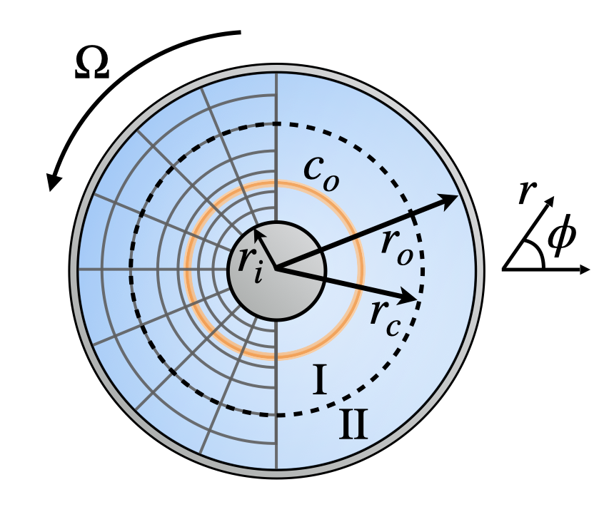
Figure 1: Schematic of the two-dimensional Taylor-Couette geometry. In the left half, the spokes-wheel mesh used in OpenFOAM^® with $N_{r}=100$ cells in the radial direction and $N_{\phi}=120$ cells in the angular direction is depicted. The radii of the inner and outer cylinders are $r_{i}=$2.5\text{\,}\mu\mathrm{m}$$ and $r_{o}=$10\text{\,}\mu\mathrm{m}$$, respectively. The outer cylinder rotates with an angular velocity $\Omega=2\pi$\text{\,}{\mathrm{s}}^{-1}$$. To investigate mixing, the area in between the cylinders is divided into two equal parts, an inner region denoted $\mathrm{I}$ with $r_{i}\leq r\leq r_{c}$ and an outer region denoted $\mathrm{II}$ with $r_{c}<r\leq r_{o}$, where $r_{c}=\sqrt{17/32}$. The initial distribution $c_{0}$ of the concentration field of a scalar, used for mixing, is displayed in orange.

2 Methods

In this section, we describe the geometry of the Taylor-Couette flow and the employed constitutive equation to model the viscoelastic fluid. Secondly, we discuss our simulation method and the simulation parameters used in this work.

2.1 Geometry and model fluid

We consider an incompressible viscoelastic fluid in a two-dimensional Taylor-Couette geometry consisting of two concentric cylinders with $r_{o}$ the radius of the outer cylinder and $r_{i}$ the radius of the inner cylinder. The outer cylinder is rotated counter-clockwise with a constant angular velocity $\Omega$ and the inner cylinder is fixed. A schematic of our set-up can be seen in fig. 1. The dynamics of the flow field $\bm{u}(\bm{r},t)$ as a function of the position $\bm{r}$ and time $t$ can be described with a generalised Navier-Stokes equation:

$$\rho\Big{(}\frac{\partial\bm{u}}{\partial t}+\bm{u}\cdot\nabla\bm{u}\Big{)}=-\nabla p+\eta_{s}\nabla^{2}\bm{u}+{\nabla\bm{\tau}}\,.$$ (1)

Here, $\rho$ is the density of the solvent, $p$ the pressure, $\eta_{s}$ the solvent shear viscosity, and ${\nabla\bm{\tau}}$ denotes the divergence of the stress tensor $\bm{\tau}$. We use the characteristic length $r_{o}$, the characteristic time $\Omega^{-1}$, and the characteristic velocity $r_{o}\Omega$ to rescale length, time, and velocity, respectively. Therefore, the Reynolds number becomes $\mathrm{Re}=\rho\Omega r_{o}^{2}/\eta_{s}$.

The additional viscoelastic stresses due to the dissolved polymers are described by the polymeric stress tensor $\bm{\tau}$, for which we choose the constitutive relation of the Oldroyd-B model oldroyd1958non ; oldroyd1950formulation :

$$\bm{\tau}+\lambda\overset{\nabla}{\bm{\tau}}=\eta_{p}\left[\nabla\otimes\bm{u}+(\nabla\otimes\bm{u})^{\mathrm{T}}\right]\,,$$ (2)

where $\eta_{p}$ is the polymeric shear viscosity and $\lambda$ the characteristic relaxation time of the dissolved polymers. Finally, $\overset{\nabla}{\bm{\tau}}$ is the upper convective derivative of the stress tensor defined as

$$\overset{\nabla}{\bm{\tau}}=\frac{\partial\bm{\tau}}{\partial t}+\bm{u}\cdot\nabla\bm{\tau}-(\nabla\otimes\bm{u})^{\mathrm{T}}\bm{\tau}-\bm{\tau}(\nabla\otimes\bm{u})\,.$$ (3)

Equations (1) and (2) can be written in dimensionless form with three relevant parameters. Besides the Reynolds number $\mathrm{Re}$, one has the ratio $\beta=\eta_{p}/\eta_{s}$ of the polymeric shear viscosity to the solvent shear viscosity and the Weissenberg number $\mathrm{Wi}=\lambda\dot{\gamma}$, where $\dot{\gamma}$ is the shear rate. For the Taylor-Couette geometry the characteristic shear rate is the angular velocity of the outer cylinder, $\dot{\gamma}\sim\Omega$, and we have $\mathrm{Wi}\simeq\lambda\Omega$.

Considering an axisymmetric flow, which corresponds to our 2D geometry, a steady and laminar solution of Eqs. (1) and (2) has been found larson1990purely . It agrees with the Taylor-Couette flow of a Newtonian fluid at low Re in the same geometry. The solution, which we denote as the base flow $\bm{u}^{0}$ and base elastic stress tensor $\bm{\tau}^{0}$ , is given by the simple shearing flow

$$u_{r}^{0}=0\,\mathchar 24635\relax\;u_{\phi}^{0}=Ar+Br^{-1}\,,$$ (4)

the stress tensor components

$$\tau_{rr}^{0}=0\,,$$ (5)

$$\tau_{r\phi}^{0}={\tau_{\phi r}^{0}=}-2\eta_{p}Br^{-2}\,,$$ (6)

$$\tau_{\phi\phi}^{0}=8\eta_{p}\lambda B^{2}r^{-4}\,,$$ (7)

and with

$$A=\frac{r^{2}_{o}}{r^{2}_{o}-r^{2}_{i}}\Omega\,\mathchar 24635\relax\;\qquad B=-r^{2}_{i}A\Omega\,.$$ (8)

To model the mixing of a solute within the fluid, we implement the advection-diffusion equation for the concentration field $c(\mathbf{r},t)$,

$$\frac{\partial c}{\partial t}+\left(\mathbf{u}\cdot\nabla\right)c=D\nabla^{2}c\,,$$ (9)

where $D$ is the molecular diffusion coefficient of the passive scalar. In the following, we neglect it by setting $D=0$. We solve the advection-diffusion equation together with the governing Eqs. (1) and (2). To solve Eq. (9), we adopt the bounded van Leer scheme for discretizing the equation, to avoid unphysical negative concentration values and lessen the effect of non-physical numerical diffusion versteeg2007 .

2.2 Simulation method and parameters

All our numerical results are obtained with the open-source finite-volume solver OpenFOAM^® for computational fluid dynamics simulations on polyhedral grids. We give all parameters in SI units, as required by OpenFOAM^®. We adopt the specialised solver for viscoelastic flows RheoTool, develop by Favero et al. favero2010 , in which the advection-diffusion equation for the concentration field $c$ is already implemented. The solver has been tested for accuracy in benchmark flows and has been shown to have second-order accuracy in space and time pimenta2017 .

Between the two coaxial cylinders of our 2D geometry, we use a grid with mesh refinement towards the inner cylinder, where velocity gradients become larger. In the left part of the geometry presented in Fig. 1, we sketch the grid mesh, which resembles a spokes wheel with $N_{r}=100$ cells in the radial direction and $N_{\phi}=120$ cells in the angular direction. The mesh refinement is such that the ratio of the radial grid size at the inner cylinder to the one at the outer cylinder is 4. The time step of the simulation is $\delta t=10^{-5}\mathrm{s}$, where the velocity, pressure, scalar concentration, and stress fields are extracted every 5000 steps. At the two bounding cylinders we choose the no-slip boundary condition for the velocity, zero gradient in the direction normal to the wall for the pressure field, and an extrapolated zero gradient in the direction normal to the wall for the polymeric stress field following Ref. pimenta2017 ; vanBuel2018elastic . We use a biconjugate gradient solver combined with a diagonal incomplete LU preconditioner (DILUP-BiCG) to solve for the components of the polymeric stress tensor and a conjugate gradient solver coupled to a diagonal incomplete Cholesky preconditioner (DIC-PCG) to solve for the velocity and pressure fields pimenta2017 .

The discretised advection-diffusion equation for the solute particles is also solved using the biconjugate gradient solver combined with a diagonal incomplete LU preconditioner, with zero gradient boundary conditions at the two bounding cylinders.

The simulations for investigating mixing are initiated with the viscoelastic fluid in the elastic turbulent state. The turbulent state is reached by starting with the fluid at rest at $\mathrm{Wi}=27.6$, where pressure, flow, and stress fields are uniformly zero, and rotating the outer cylinder for $t=250$ rotations. Then, the Weissenberg number is lowered to the desired value. This approach is also used when determining the order parameter for decreasing $\mathrm{Wi}$ in Sec. 3.1; for increasing $\mathrm{Wi}$ we just choose the specific value of $\mathrm{Wi}$ and proceed with the outlined protocol. The following geometric parameters are chosen from the viewpoint of microfluidic settings in such a way as to set a low Reynolds number. We adjust the Weissenberg number by varying the polymeric relaxation time $\lambda$. We set the polymeric shear viscosity to $\eta_{p}=0.0015\,{\mathrm{kg\,m^{-1}\,s^{-1}}}$, the solvent shear viscosity to $\eta_{s}=0.001\,{\mathrm{kg\,m^{-1}s^{-1}}}$, and the density to $\rho=1000\,\mathrm{kg/m^{3}}$. The ratio of the polymeric to the solvent viscosity is then $\beta={\eta_{p}}/{\eta_{s}}=1.5$. Thus, the Reynolds number becomes $\mathrm{Re}=0.628\cdot 10^{-3}$. The fluid flow is simulated up to ${600}\mskip 3.0mu\mathrm{s}$.

3 Results

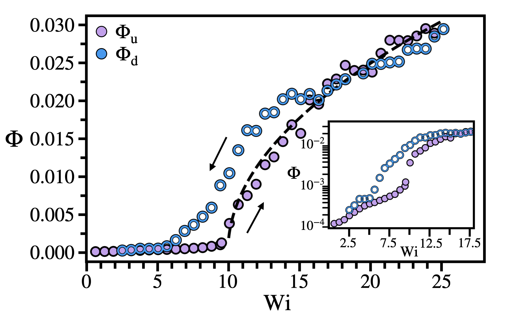
Figure 2: Order parameter $\Phi$ versus the Weissenberg number $\mathrm{Wi}$, initiated from rest ($\Phi_{\mathrm{u}}$) or from the turbulent state ($\Phi_{\mathrm{d}}$). Hysteresis is observed between $\mathrm{Wi}\approx 5.5$ and $\mathrm{Wi}\approx 16$. The upward and downward arrow in the plot indicate an increase and decrease in $\mathrm{Wi}$ compared to the initial state, respectively. The dashed line gives the scaling relation $\Phi\sim(\mathrm{Wi}-\mathrm{Wi_{c}})^{\gamma}$ with $\gamma=0.495$ and $\mathrm{Wi_{c}}=9.95$. Inset: In the semi-logarithmic plot a small jump of $\Phi_{\mathrm{u}}$ is observed.

First, we characterise the different flow states using an order parameter. Then, we address mixing in a viscoelastic fluid by analysing the spreading of a passive scalar such as solutes in the different flow states. Finally, we introduce three measures to characterise the degree of mixing of the scalar field.

3.1 Subcritical transition to elastic turbulence

As in our earlier work vanBuel2018elastic , we take the secondary-flow strength

$$\sigma(t)\equiv\left.\sqrt{\left\langle[\bm{u}(\bm{r},t)-\bm{u}^{0}(\bm{r})]^{2}\right\rangle}\right/u^{0}_{\mathrm{max}}\,,$$ (10)

as a measure for the velocity fluctuations of the flow field about the base flow $\bm{u^{0}}(\bm{r})$ and define an order parameter, $\Phi=\overline{\sigma}$, as its time average. Here, $\langle\dots\rangle$ denotes a volume average performed over the radial and angular coordinate and $u^{0}_{\mathrm{max}}$ is the velocity of the outer cylinder.

The order parameter is plotted in Fig. 2 as a function of the Weissenberg number. Two different initial conditions are used: one, where the fluid starts from rest ($\Phi_{\mathrm{u}}$), and one, where the fluid starts from the turbulent flow state at a high Weissenberg number, which then is subsequently lowered ($\Phi_{\mathrm{d}}$). For both initial conditions the flow is equilibrated during 100 rotations. This ensures that the secondary flow strength $\sigma(t)$ fluctuates about a steady value. Then, the order parameter is obtained from $\sigma(t)$ by averaging over another 400 - 500 rotations.

In the case where the fluid starts at rest, a continuous transition from the laminar base flow to the elastic turbulent state is observed at a critical Weissenberg number $\mathrm{Wi_{c}}=9.95$. Analogous to our earlier work vanBuel2018elastic , we determined the power spectra of the velocity fluctuations and identified the turbulent state from the steepness of the observed power-law decay (data not shown). In the case where the fluid starts from the turbulent state and upon decreasing $\mathrm{Wi}$, the order parameter evolves continuously from the elastic turbulent flow state ($\Phi_{\mathrm{d}}>0.007$) to a weakly-chaotic state ($0<\Phi_{\mathrm{d}}<0.007$), and to the laminar base flow ($\Phi_{\mathrm{d}}\approx 0$). The observation of the weakly-chaotic flow state below $\mathrm{Wi_{c}}$ is similar to our results in the von Kármán flow vanBuel2022characterizing .

Most importantly, we find hysteretic behaviour in the order parameter, where $\Phi_{\mathrm{d}}>\Phi_{\mathrm{u}}$ between $\mathrm{Wi}\approx 5.5$ and $\mathrm{Wi}\approx 16$, and a small jump in the order parameter is observed for increasing $\mathrm{Wi}$ (see inset of Fig. 2). Thus, we conclude that the nature of the transition from laminar to turbulent flow is subcritical, in contrast to our earlier findings in Ref. vanBuel2018elastic , where we did not check for hysteresis. A detailed account of our study will be published elsewhere.

3.2 Mixing in viscoelastic fluids

An interesting application of viscoelastic fluids is to utilise elastic turbulence at low Reynolds numbers for mixing solutes in a fluid or mixing of multiple fluids, which results in a homogenised fluid. As a first approach we investigate the mixing of a passive scalar in the two-dimensional Taylor-Couette flow.

We start from the turbulent flow state, obtained at $\mathrm{Wi}=27.6$ after 250 rotations, without any scalar quantity present in the fluid. Then, we lower the Weissenberg number to the desired value and let the viscoelastic fluid flow equilibrate for another 100 rotations. At this point, denoted time $t=0$, the scalar field is initialised with concentration $c_{0}$ on a ring with radius $r=0.432\,r_{o}$ and a width equal to the local grid spacing. The initial scalar field is chosen close to the inner cylinder, where the radial velocity fluctuations, due to the increased hoop stress, are large. Afterwards, the fluid flow is evolved for an additional 400 to 500 rotations. The order parameter $\Phi_{\mathrm{d}}$ corresponding to these Weissenberg numbers is given by the blue circles in Fig. 2.

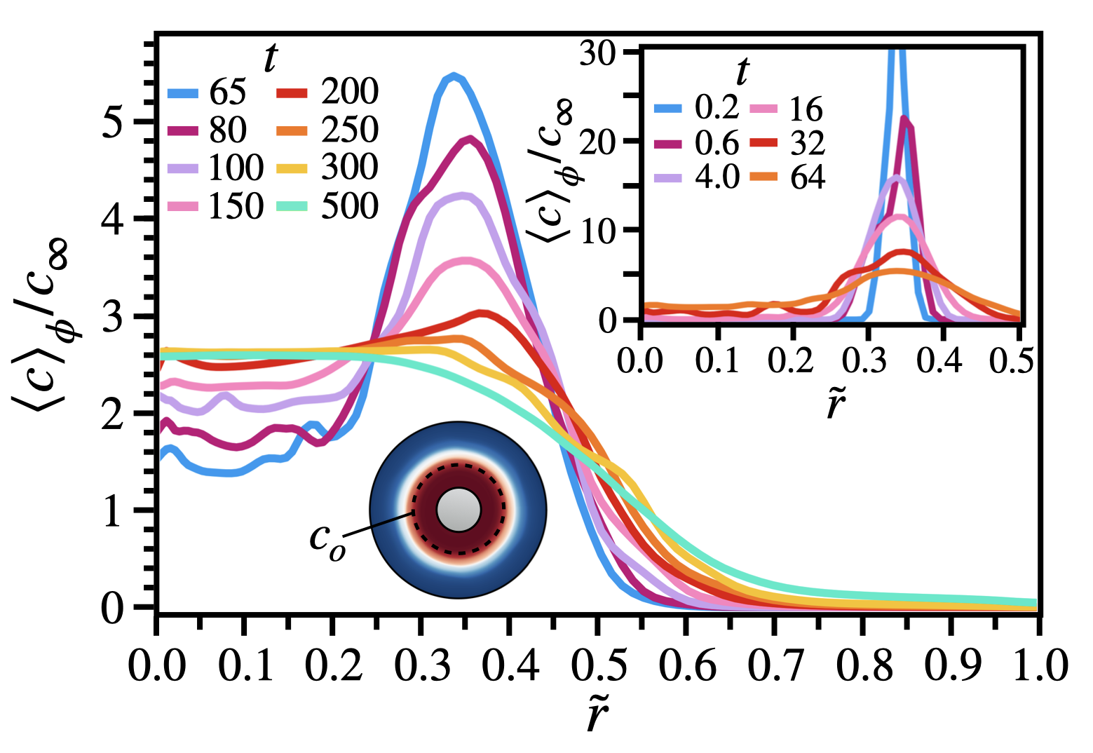
Figure 3: Averaged normalised concentration field of the passive scalar $\langle c\rangle_{\phi}/c_{\infty}$ plotted versus the normalised radial position $\tilde{r}=(r-r_{i})/(r_{o}-r_{i})$, where the averaging is over the azimuthal direction $\phi$, $c_{\infty}$ is the concentration of the completely mixed state. The profiles are shown for different times $t$ at $\mathrm{Wi}=10.68$, with early times in the top right inset. The bottom left inset displays a snapshot of the concentration field at $t=598$. The dashed ring indicates the initial position of the scalar field.

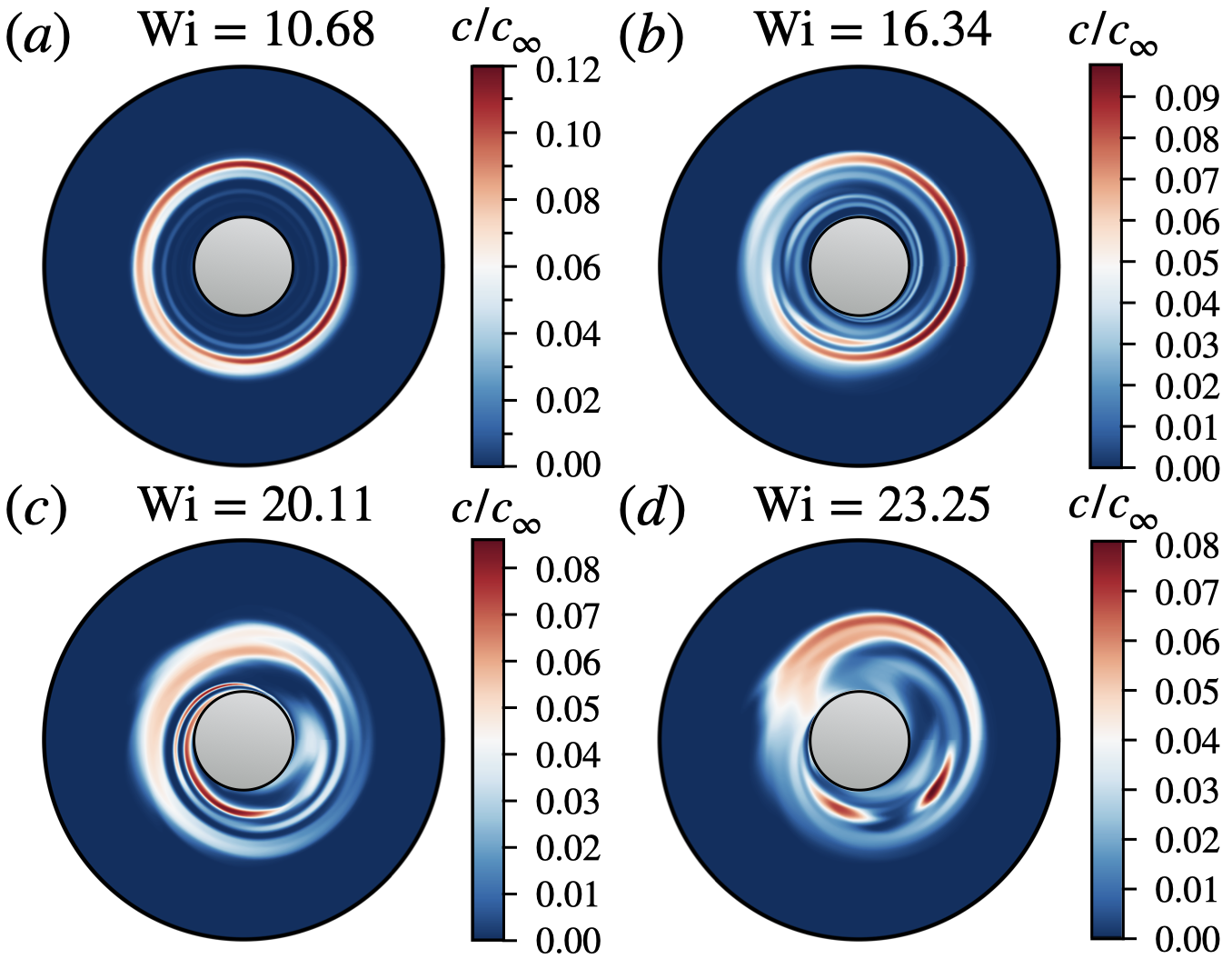
Figure 4: Snapshots of the normalised concentration field $c(r,\phi)/c_{\infty}$ for (a) $\mathrm{Wi}=10.68$, (b) $\mathrm{Wi}=16.34$, (c) $\mathrm{Wi}=20.11$ and (d) $\mathrm{Wi}=23.25$ at time $t=16$.

In Fig. 3 we plot the azimuthally averaged concentration field $\langle c(r,t)\rangle_{\phi}$ versus the normalised radial position $\tilde{r}=(r-r_{i})/(r_{o}-r_{i})$ at different times in the elastic turbulent regime at $\mathrm{Wi}=10.68$, where

$$\langle c(r,t)\rangle_{\phi}=\frac{1}{2\pi}\int_{0}^{2\pi}c(\mathbf{r},t)d\phi\,.$$ (11)

The concentration field is normalised by the concentration of a uniformly distributed solute, $c_{\infty}=A^{-1}\int_{A}c(\mathbf{r},t)dA$, where $A$ is the area between the two cylinders. Initially, the strongly peaked distribution spreads quickly along the radial direction towards the inner cylinder (see inset of Fig. 3). Moreover, for increasing $\mathrm{Wi}$ we find that the concentration field spreads faster towards the inner cylinder because velocity fluctuations become stronger. This is illustrated in Fig. 4, where we plot snapshots of the concentration field at time $t=16$ for (a) $\mathrm{Wi}=10.68$, (b) $\mathrm{Wi}=16.34$, (c) $\mathrm{Wi}=20.11$ and (d) $\mathrm{Wi}=23.25$. The figure shows how the concentration field is folded inwards by radial flow, which results in a spiral pattern of the concentration field. Random fluctuations in the radial velocity field lead to significantly different spreading of $c$ at different $\mathrm{Wi}$. Overall, the figure clearly demonstrates the initial rapid and random mixing for increasing $\mathrm{Wi}$. With increasing time the concentration field becomes more evenly distributed in the region near the inner cylinder and a step-like profile develops (see Fig. 3). Here, mixing slows down and at long times the concentration field develops towards a uniform distribution where $c=c_{\infty}$. A snapshot of the concentration field for $\mathrm{Wi}=10.68$ at $t=598$ is shown in the bottom inset of Fig. 3.

We characterise the degree of mixing by the standard deviation of the concentration field normalised by its initial value,

$$\Delta c\equiv\sqrt{\frac{\langle[c(\mathbf{r},t)-c_{\infty}]^{2}\rangle}{\langle[c(\mathbf{r},0)-c_{\infty}]^{2}\rangle}}\,,$$ (12)

where $\langle g\rangle={A}^{-1}\int_{A}g\,dA$ indicates an average of $g$ over the area $A$ between the two cylinders. The normalised standard deviation $\Delta c$ is such that initially $\Delta c=1$ and $\Delta c=0$ for the completely mixed state with $c=c_{\infty}$.

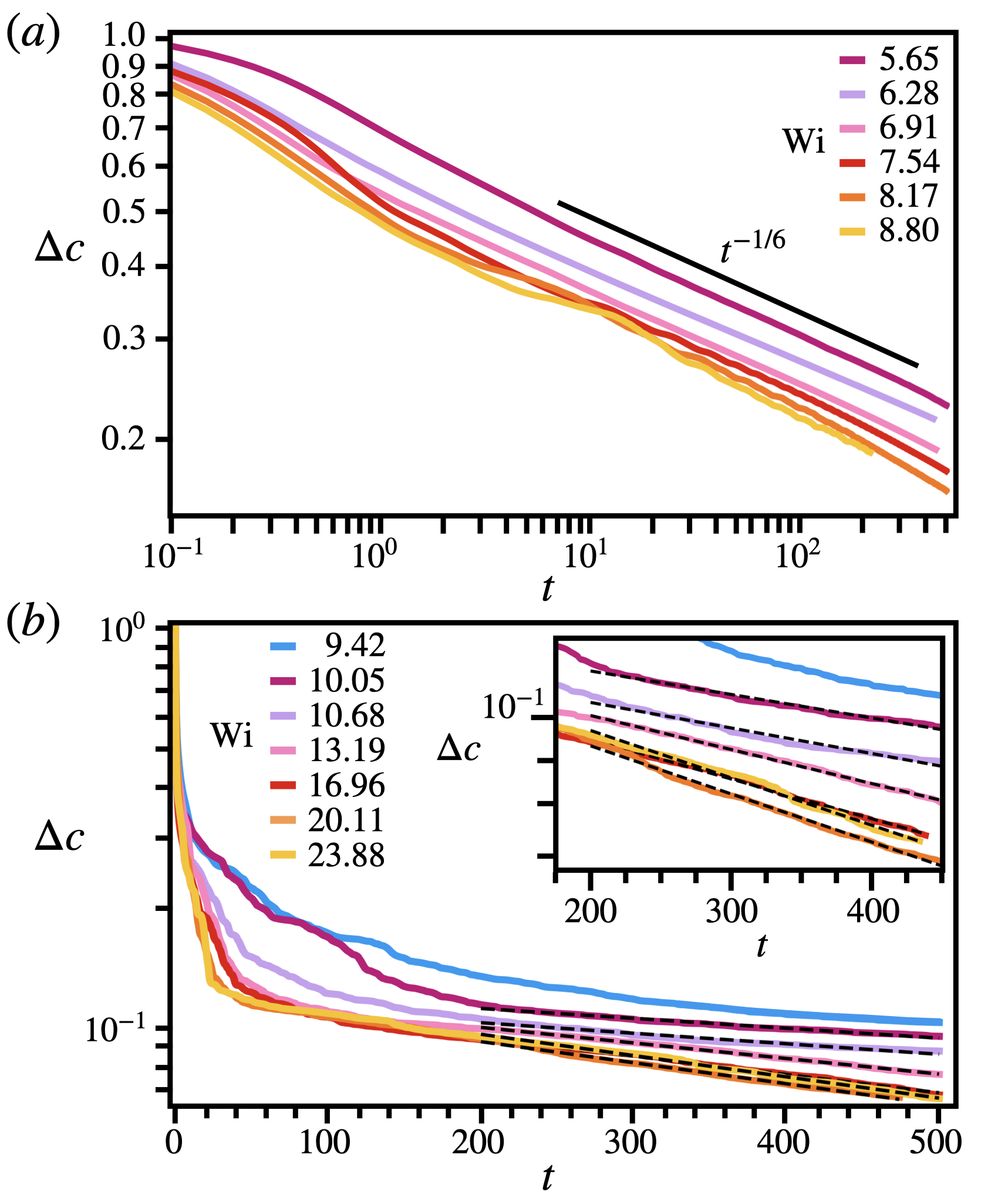
Figure 5: Normalised standard deviation of the concentration field $\Delta c$ plotted versus time $t$ at (a) Weissenberg numbers $5.65{\leq}\mathrm{Wi}\leq 8.80$ corresponding to the weakly-chaotic state and at (b) Weissenberg numbers $\mathrm{Wi}\geq{9.42}$, in the elastic turbulent state. In (a) power-law scaling is observed with an exponent close to $-1/6$. In (b) fits with the exponential function $\exp(-\alpha_{\mathrm{mix}}t)$ are indicated by the dashed lines, where $\alpha_{\mathrm{mix}}$ denotes the mixing rate. Inset: Close-up of the exponential fits.

In the laminar case ($\mathrm{Wi}<5.03$), mixing is completely governed by diffusion, which in the present work is neglected ($D=0$). In the regime of weakly-chaotic flow, velocity fluctuations are increased, the velocity spectrum displays pronounced peaks and no power-law scaling is observed, hence, elastic turbulence does not occur (see Fig. 2). In Fig. 5 (a) we plot the standard deviation of the concentration field $\Delta c$ versus time $t$ for Weissenberg numbers $5.03<\mathrm{Wi}\leq 8.17$, i.e., in the weakly-chaotic flow state. Initially, the standard deviation decreases stronger at larger $\mathrm{Wi}$ since the fluctuations in the flow field are larger. Then, for all values of $\mathrm{Wi}$ the standard deviation enters power-law scaling with an exponent close to $-1/6$. The unsteady flow in the weakly chaotic flow regime yields chaotic advection aref1984stirring ; ottino1989kinematics . Thus, the enhanced fluctuations in the velocity field increase mixing within the fluid.

In Fig. 5 (b) we plot $\Delta c$ versus time $t$ for Weissenberg numbers $\mathrm{Wi}\geq 9.42$ in the elastic turbulent state. We observe an initial rapid mixing due to the broadening of the initial concentration ring as illustrated in the inset of Fig. 3. This is followed by a slower exponential mixing, when the concentration has developed the step-like distribution, which then broadens (see Fig. 3). For the four highest $\mathrm{Wi}$ presented in the plot, the change from rapid to slower mixing occurs rather abruptly between $t=20$ and $30$. We can fit the slower mixing by an exponential decay, $\Delta c\sim\exp(-\alpha_{\mathrm{mix}}t)$, where $\alpha_{\mathrm{mix}}$ is the mixing rate. The fits are indicated with the black dashed lines, which start at $t=200$ for all $\mathrm{Wi}$. We have chosen the fitting starting time such that all slopes of the standard deviation in the elastic turbulent regime can be well fitted by an exponential tail. Moreover, increasing the fitting range for larger Wi does not alter the results. The inset of Fig. 5 shows a close-up of the exponential fits.

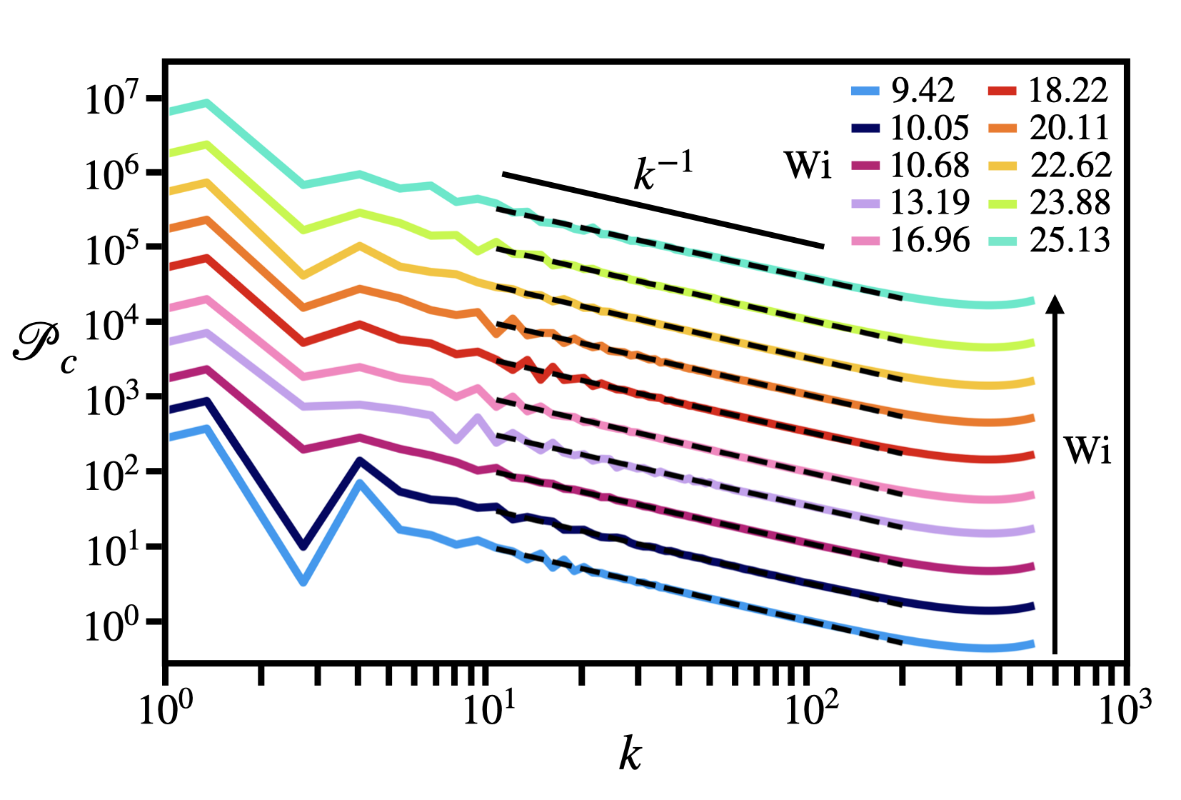
Figure 6: Radial power spectral density ${\mathcal{P}_{c}}(k)$ of the scalar concentration field as a function of the radial wave number $k$ for different $\mathrm{Wi}$ at time $t=550$. The data are arbitrarily offset by half a decade for clarity. Power laws $k^{-\alpha}$ are fitted and plotted as black dashed lines in the range $10\leq k\leq 100$ in the elastic turbulent regime.

The exponential scaling observed in the standard deviation suggests mixing within the fluid occurs in the Batchelor regime. To further investigate this, we compute the radial power spectral density of the concentration field following Ref. pierrehumbert2000batchelor . We start by introducing the Fourier transform in polar coordinates: $\hat{c}(\mathbf{k})=\mathcal{F}\{c\}(\mathbf{k})$, where the wave vector $\mathbf{k}$ is represented by the radial wave number $k$ and the polar angle $\theta$. In order to perform the Fourier transform in the radial direction, which requires a regular radial spacing of the grid, the concentration field is approximated by a cubic spline fit with constant spacing. Then, averaging over the azimutal direction due to the cylindrical symmetry and performing an average over time, the radial power spectrum of the concentration field is obtained as pierrehumbert2000batchelor

$$\mathcal{P}_{c}(k)=\frac{1}{(2\pi)^{2}\Delta t}\int_{t_{0}}^{t_{1}}\int_{0}^{2\pi}\lvert\hat{c}(\mathbf{k})\rvert^{2}kd\theta dt\,,$$ (13)

where $\overline{x}$ denotes a time average of $x$. The power spectrum $\mathcal{P}_{c}(k)$ is plotted in Fig. 6. The time interval for the average is $550\leq t\leq 600$. We observe a Batchelor spectrum with power scaling $k^{-1}$ in the elastic turbulent regime, $\mathrm{Wi}\geq 9.42$, which is also observed in experiments groisman2001efficient .

Now, we take a closer look at the mixing rate and how it relates to the order parameter. In Fig. 7 (a) we plot both the order parameter $\Phi_{\mathrm{d}}$, obtained before in Fig. 2, and the mixing rate $\alpha_{\mathrm{mix}}$, obtained from the fits in Fig. 5 (b). We observe a strong correlation between $\alpha_{\mathrm{mix}}$ and $\Phi_{\mathrm{d}}$, which indicates that increased velocity fluctuations increase the mixing within the fluid. Since mixing below $\mathrm{Wi}<9$ follows algebraic scaling, a mixing rate cannot be determined and is not included in the plot. We conclude that our order parameter is therefore also a good measure for mixing within the fluid.

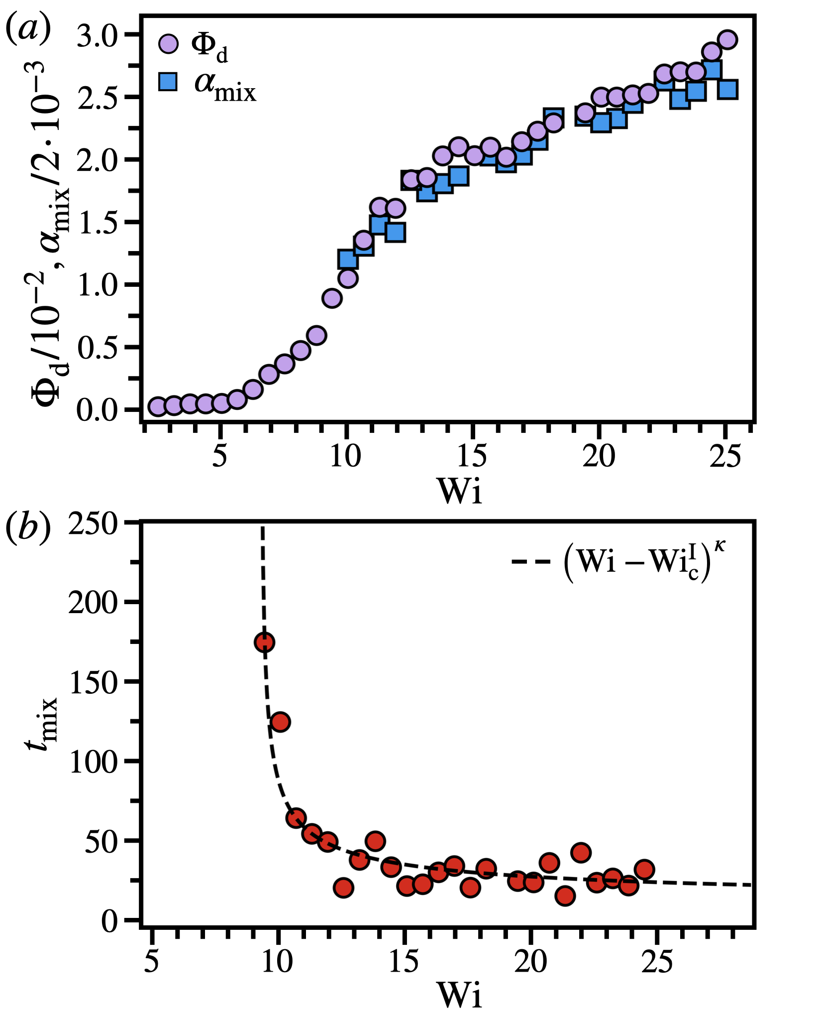
Figure 7: (a) Order parameter $\Phi_{\mathrm{d}}$ and the mixing rate $\alpha_{\mathrm{mix}}$ versus the Weissenberg number $\mathrm{Wi}$. (b) Mixing time $t_{\mathrm{m}}$ versus the Weissenberg number $\mathrm{Wi}$. The dashed line indicates the scaling law $(\mathrm{Wi}-\mathrm{Wi_{c}^{I}})^{\kappa}$, with $\mathrm{Wi_{c}^{I}}=9.26\pm 0.04$ and $\kappa=-0.52\pm 0.03$.

Moreover, we define a mixing time from the standard deviation of the concentration field. We determine the fluid to be well-mixed when the standard deviation is small, $\Delta c\approx 0.14$, and define the mixing time $t_{\mathrm{mix}}$, when this value is reached. It was chosen such that $\Delta c$ in the elastic turbulent state falls below 0.14 within the total simulation time, while this value is not reached in the weakly-chaotic state occurring below $\mathrm{Wi}<9.4$. In Fig. 7 (b) we plot the mixing time versus $\mathrm{Wi}$. The figure shows a strong decrease in $t_{\mathrm{mix}}$ with increasing $\mathrm{Wi}$. The mixing time in the turbulent regime at $\mathrm{Wi}\geq 9.4$ roughly follows the scaling $t_{\mathrm{mix}}\sim\left(\mathrm{Wi}-\mathrm{Wi_{c}^{I}}\right)^{-1/2}$ with $\mathrm{Wi_{c}^{I}}={9.26}$. The mixing time includes both the rapid initial mixing and the slow mixing afterwards. It is sensitive to fluctuations during the initial rapid mixing, where random velocity fluctuations in the radial directions have a large impact on the overall mixing time. Thus, it exhibits large variations. Nevertheless, in total a strong decrease in the mixing time is observed in the turbulent flow state, which demonstrates the impact of elastic turbulence on mixing.

Lastly, we determine the degree of mixing by examining the concentration that develops in a specific region. To this end, we divide the Taylor-Couette geometry into two equal areas: the inner region (region $\mathrm{I}$), near the inner cylinder with $r_{i}<r<r_{c}$ and the outer region (region $\mathrm{II}$), near the outer cylinder with $r_{c}<r<r_{o}$. The dividing radius $r_{c}$ is determined from the condition of equal areas and thus is given by $r_{c}=\sqrt{17/32}{\,r_{o}}\approx 0.73{\,r_{0}}$. Initially, the passive scalar is located in the inner region. Therefore, we consider the developing concentration in the outer region $\mathrm{II}$ as a good indicator for the degree of mixing. In Fig. 8 we plot the normalised concentration $c^{\mathrm{II}}/c_{\infty}$ in region $\mathrm{II}$ as a function of the Weissenberg number. The concentration is averaged over region II and between times $t=400$ and $t=500$, which is chosen such that it is large enough to give an accurate average value, but not too large such that the concentration varies significantly (see Fig. 5). We again observe scaling behaviour, where $c^{\mathrm{II}}\sim(\mathrm{Wi}-\mathrm{Wi^{I}_{c}})^{\gamma}$ with $\gamma=0.28\pm 0.03$ and $\mathrm{Wi_{c}^{I}}=9.26$. Comparing with the scaling we found for $t_{\mathrm{mix}}$, we thus obtain the scaling relation $c^{\,\mathrm{II}}\sim t_{\mathrm{mix}}^{-1/2}$. We checked that his scaling relation does not depend on varying the initial time of the averaging time interval between 250 and 450.

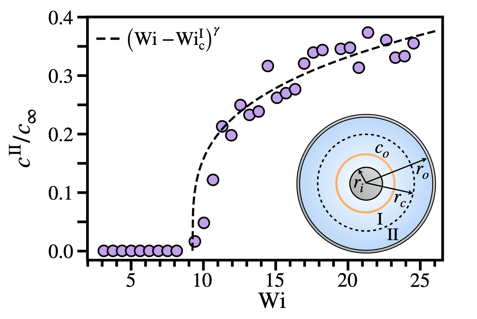
Figure 8: Normalised concentration $c/c_{\infty}$ in region II (see inset or Fig. 1) averaged between times $t=400$ and $t=500$. The dashed line shows the scaling law $(\mathrm{Wi}-\mathrm{Wi_{c}})^{\gamma}$ with $\mathrm{Wi_{c}^{I}}=9.26$ and $\gamma=0.28\pm 0.03$.

4 Conclusion

We have investigated how advection by the flow field of elastic turbulence determines mixing within a viscoelastic fluid in a two-dimensional Taylor-Couette flow. For this we used numerical solutions of the Oldroyd-B model with the program OpenFOAM^®. The Weissenberg number is varied while keeping the Reynolds number very small and constant. In contrast to our earlier work vanBuel2018elastic , we identified the transition towards elastic turbulence as a subcritical transition. When lowering the Weissenberg number, elastic turbulence continues to exist below the critical Weissenberg number $\mathrm{Wi}_{c}=9.95$, determined earlier for increasing $\mathrm{Wi}$ vanBuel2018elastic . Then, below $\mathrm{Wi_{c}^{I}}=9.26$ a weakly-chaotic flow occurs, which ultimately becomes laminar for $\mathrm{Wi}\leq 5.03$.

The turbulent and weakly-chaotic secondary flows have non-zero radial components, which is ideal for mixing at the micrometer scale. Chaotic advection in the weakly-chaotic flow state causes mixing, where the standard deviation of the concentration field shows power-law scaling. The elastic turbulent state displays strong initial mixing followed by a slower exponential decay in the standard deviation. The exponential decay corresponds to the regime of Batchelor mixing, also observed in experiments on mixing in elastic turbulence groisman2001efficient . The exponential decay or the mixing rate coincides with the secondary-flow order parameter. Finally, for the elastic turbulent state we also introduced a mixing time and mixing efficiency, which follow scaling laws.

Our numerical work confirms that elastic turbulence can be harnessed for mixing a passive scalar in viscoelastic fluids at very low Reynolds numbers and the Batchelor regime is identified, both results are also observed in experiments groisman2001efficient ; groisman2004elastic . Moreover, we have demonstrated that the secondary-flow order parameter is strongly correlated to the mixing rate and hence it is also a good indication for the degree of flow-induced mixing.

Acknowledgments

We acknowledge support from the Deutsche Forschungsgemeinschaft in the framework of the Collaborative Research Center SFB 910.

Author contribution statement

All authors contributed equally to this work.

Declarations

Conflict of Interest

The authors have no conflicts to disclose.

Data Availability Statement

The data that support the findings of this study are available from the corresponding author upon reasonable request.

References

- \bibcommenthead
- (1) Groisman, A., Steinberg, V.: Elastic turbulence in a polymer solution flow. Nature 405(6782), 53 (2000)
- (2) Groisman, A., Steinberg, V.: Efficient mixing at low reynolds numbers using polymer additives. Nature 410(6831), 905 (2001)
- (3) Groisman, A., Steinberg, V.: Elastic turbulence in curvilinear flows of polymer solutions. New J. Phys. 6(1), 29 (2004)
- (4) Burghelea, T., Segre, E., Bar-Joseph, I., Groisman, A., Steinberg, V.: Chaotic flow and efficient mixing in a microchannel with a polymer solution. Phys. Rev. E 69(6), 066305 (2004)
- (5) Burghelea, T., Segre, E., Steinberg, V.: Mixing by polymers: Experimental test of decay regime of mixing. Phys. Rev. Lett. 92(16), 164501 (2004)
- (6) Thomases, B., Shelley, M.: Transition to mixing and oscillations in a Stokesian viscoelastic flow. Phys. Rev. Lett. 103(9), 094501 (2009)
- (7) Thomases, B., Shelley, M., Thiffeault, J.-L.: A stokesian viscoelastic flow: transition to oscillations and mixing. Physica D 240(20), 1602–1614 (2011)
- (8) Kumar, S., Homsy, G.: Chaotic advection in creeping flow of viscoelastic fluids between slowly modulated eccentric cylinders. Phys. Fluids 8(7), 1774–1787 (1996)
- (9) Niederkorn, T., Ottino, J.M.: Mixing of a viscoelastic fluid in a time-periodic flow. J. Fluid Mech. 256, 243–268 (1993)
- (10) Arratia, P.E., Thomas, C.C., Diorio, J., Gollub, J.P.: Elastic instabilities of polymer solutions in cross-channel flow. Phys. Rev. Lett. 96(14), 144502 (2006)
- (11) Burghelea, T., Segre, E., Steinberg, V.: Elastic turbulence in von karman swirling flow between two disks. Phys. Fluids 19(5), 053104 (2007)
- (12) Jun, Y., Steinberg, V.: Polymer concentration and properties of elastic turbulence in a von karman swirling flow. Phys. Rev. Fluids 2(10), 103301 (2017)
- (13) van Buel, R., Schaaf, C., Stark, H.: Elastic turbulence in two-dimensional taylor-couette flows. Europhys. Lett. 124(1), 14001 (2018)
- (14) Squires, T.M., Quake, S.R.: Microfluidics: Fluid physics at the nanoliter scale. Rev. Mod. Phys. 77(3), 977 (2005)
- (15) Balkovsky, E., Fouxon, A., Lebedev, V.: Turbulence of polymer solutions. Phys. Rev. E 64(5), 056301 (2001)
- (16) Larson, R.G., Shaqfeh, E.S.G., Muller, S.J.: A purely elastic instability in Taylor-Couette flow. J. Fluid Mech. 218, 573–600 (1990)
- (17) McKinley, G.H., Byars, J.A., Brown, R.A., Armstrong, R.C.: Observations on the elastic instability in cone-and-plate and parallel-plate flows of a polyisobutylene boger fluid. J. Non-Newtonian Fluid Mech. 40(2), 201–229 (1991)
- (18) Byars, J.A., Öztekin, A., Brown, R.A., Mckinley, G.H.: Spiral instabilities in the flow of highly elastic fluids between rotating parallel disks. J. Fluid Mech. 271, 173–218 (1994)
- (19) Ducloué, L., Casanellas, L., Haward, S.J., Poole, R.J., Alves, M.A., Lerouge, S., Shen, A.Q., Lindner, A.: Secondary flows of viscoelastic fluids in serpentine microchannels. Microfluid. Nanofluid. 23(3), 33 (2019)
- (20) Pakdel, P., McKinley, G.H.: Elastic instability and curved streamlines. Phys. Rev. Lett. 77(12), 2459 (1996)
- (21) Varshney, A., Steinberg, V.: Drag enhancement and drag reduction in viscoelastic flow. Phys. Rev. Fluids 3(10), 103302 (2018)
- (22) Jun, Y., Steinberg, V.: Power and pressure fluctuations in elastic turbulence over a wide range of polymer concentrations. Phys. Rev. Lett. 102(12), 124503 (2009)
- (23) Sousa, P.C., Pinho, F.T., Alves, M.A.: Purely-elastic flow instabilities and elastic turbulence in microfluidic cross-slot devices. Soft Matter 14(8), 1344–1354 (2018)
- (24) Steinberg, V.: Scaling relations in elastic turbulence. Phys. Rev. Lett. 123(23), 234501 (2019)
- (25) Groisman, A., Steinberg, V.: Stretching of polymers in a random three-dimensional flow. Phys. Rev. Lett. 86(5), 934 (2001)
- (26) Berti, S., Boffetta, G.: Elastic waves and transition to elastic turbulence in a two-dimensional viscoelastic kolmogorov flow. Phys. Rev. E 82(3), 036314 (2010)
- (27) Canossi, D.O., Mompean, G., Berti, S.: Elastic turbulence in two-dimensional cross-slot viscoelastic flows. Europhys. Lett. 129(2), 24002 (2020)
- (28) Steinberg, V.: Elastic turbulence: an experimental view on inertialess random flow. Annu. Rev. Fluid Mech. 53, 27–58 (2021)
- (29) Morozov, A.N., van Saarloos, W.: Subcritical finite-amplitude solutions for plane Couette flow of viscoelastic fluids. Phys. Rev. Lett. 95(2), 024501 (2005)
- (30) Pan, L., Morozov, A., Wagner, C., Arratia, P.E.: Nonlinear elastic instability in channel flows at low Reynolds numbers. Phys. Rev. Lett. 110(17), 174502 (2013)
- (31) Poole, R.J., Alves, M.A., Oliveira, P.J.: Purely elastic flow asymmetries. Phys. Rev. Let.. 99(16), 164503 (2007)
- (32) Varshney, A., Steinberg, V.: Elastic wake instabilities in a creeping flow between two obstacles. Phys. Rev. Fluids 2(5), 051301 (2017)
- (33) Berti, S., Bistagnino, A., Boffetta, G., Celani, A., Musacchio, S.: Two-dimensional elastic turbulence. Phys. Rev. E 77(5), 055306 (2008)
- (34) Shaqfeh, E.S.: Purely elastic instabilities in viscometric flows. Annu. Rev. Fluid Mech. 28(1), 129–185 (1996)
- (35) Joo, Y.L., Shaqfeh, E.S.G.: Observations of purely elastic instabilities in the Taylor–Dean flow of a Boger fluid. J. Fluid Mech. 262, 27–73 (1994)
- (36) Sureshkumar, R., Beris, A.N., Avgousti, M.: Non-axisymmetric subcritical bifurcations in viscoelastic Taylor–Couette flow. Proc. R. Soc. Lond. A 447(1929), 135–153 (1994)
- (37) Poole, R., Budhiraja, B., Cain, A., Scott, P.: Emulsification using elastic turbulence. Journal of Non-Newtonian Fluid Mechanics 177, 15–18 (2012)
- (38) Yang, H., Yao, G., Wen, D.: Experimental investigation on convective heat transfer of shear-thinning fluids by elastic turbulence in a serpentine channel. Experimental Thermal and Fluid Science 112, 109997 (2020)
- (39) Gupta, S., Chauhan, A., Sasmal, C.: Influence of elastic instability and elastic turbulence on mixed convection of viscoelastic fluids in a lid-driven cavity. International Journal of Heat and Mass Transfer 186, 122469 (2022)
- (40) Grilli, M., Vázquez-Quesada, A., Ellero, M.: Transition to turbulence and mixing in a viscoelastic fluid flowing inside a channel with a periodic array of cylindrical obstacles. Phys. Rev. Lett. 110(17), 174501 (2013)
- (41) van Buel, R., Stark, H.: Active open-loop control of elastic turbulence. Sci. Rep. 10(1), 1–9 (2020)
- (42) van Buel, R., Stark, H.: Characterizing elastic turbulence in the three-dimensional von kármán swirling flow using the oldroyd-b model. Phys. Fluids 34(4), 043112 (2022)
- (43) Oldroyd, J.G.: Non-Newtonian effects in steady motion of some idealized elastico-viscous liquids. Proc. R. Soc. Lond. A 245(1241), 278–297 (1958)
- (44) Oldroyd, J.G.: On the formulation of rheological equations of state. Proc. R. Soc. Lond. A 200(1063), 523–541 (1950)
- (45) Versteeg, H.K., Malalasekera, W.: An Introduction to Computational Fluid Dynamics: the Finite Volume Method, 2nd edn. Pearson Education Limited, Edinburgh Gate, Harlow, England (2007)
- (46) Favero, J.L., Secchi, A.R., Cardozo, N.S.M., Jasak, H.: Viscoelastic fluid analysis in internal and in free surface flows using the software OpenFOAM. Comput. Chem. Eng. 34(12), 1984–1993 (2010)
- (47) Pimenta, F., Alves, M.A.: Stabilization of an open-source finite-volume solver for viscoelastic fluid flows. J. Non-Newtonian Fluid Mech. 239, 85–104 (2017)
- (48) Aref, H.: Stirring by chaotic advection. Journal of fluid mechanics 143, 1–21 (1984)
- (49) Ottino, J.M.: The Kinematics of Mixing: Stretching, Chaos, and Transport vol. 3. Cambridge university press, ??? (1989)
- (50) Pierrehumbert, R.: The batchelor spectrum and tracer cascade. Ct2, 90 (2000)