Offline Task Assistance Planning on a Graph:
Theoretic and Algorithmic Foundations
Abstract
In this work we introduce the problem of task assistance planning where we are given two robots and . The first robot, , is in charge of performing a given task by executing a precomputed path. The second robot, , is in charge of assisting the task performed by using on-board sensors. The ability of to provide assistance to depends on the locations of both robots. Since is moving along its path, may also need to move to provide as much assistance as possible. The problem we study is how to compute a path for so as to maximize the portion of ’s path for which assistance is provided. We limit the problem to the setting where moves on a roadmap which is a graph embedded in its configuration space and show that this problem is -hard. Fortunately, we show that when moves on a given path, and all we have to do is compute the times at which should move from one configuration to the following one, we can solve the problem optimally in polynomial time. Together with carefully-crafted upper bounds, this polynomial-time algorithm is integrated into a Branch and Bound-based algorithm that can compute optimal solutions to the problem outperforming baselines by several orders of magnitude. We demonstrate our work empirically in simulated scenarios containing both planar manipulators and UR robots as well as in the lab on real robots.
Keywords:
Motion and Path Planning Algorithmic Completeness and Complexity.1 Introduction
In this work we introduce the problem of task assistance planning (TAP) where we are given two robots and . The first robot, , which we call the task robot, is in charge of performing a given task by executing a precomputed path. The second robot, , which we call the assistance robot, is in charge of assisting the task performed by using on-board sensors.111 Importantly, by assistance we mean assistance that does not affect the task itself such as communication, micro-control and visual monitoring. The ability of to provide assistance to depends on the locations of both robots. Since is moving along its path, may also need to move to provide as much assistance as possible. In its simplest form, the problem calls for computing a path for so as to maximize the portion of ’s path for which assistance is provided.
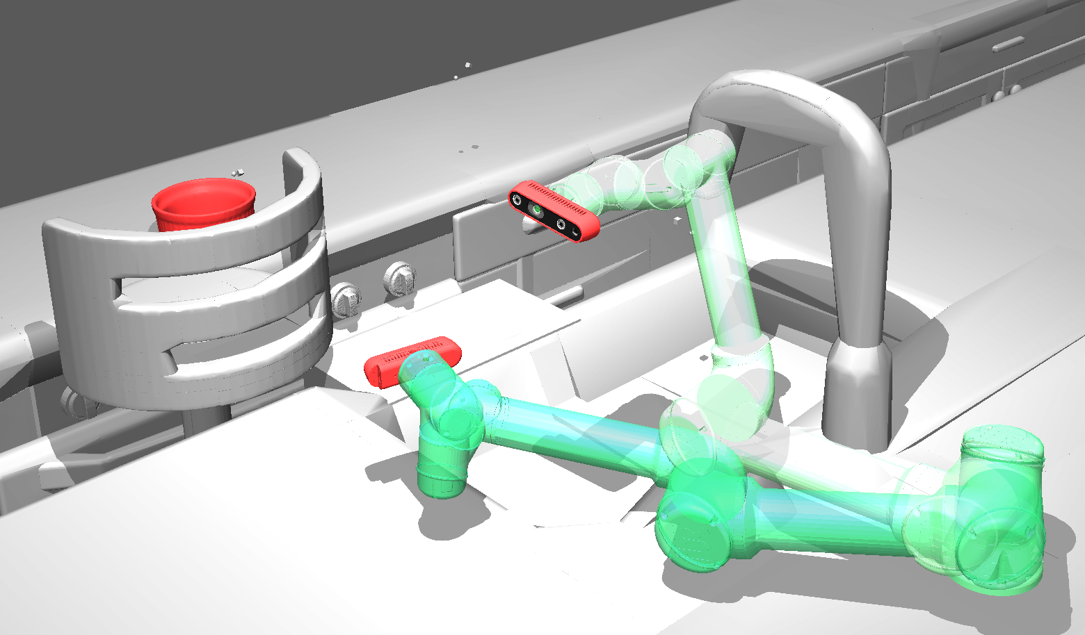
Examples of assistance include visual feedback and communication relays. For example, visual feedback can be used within the feedback loop of a low-level controller as demonstrated in Fig. 1. Here, a controller is used to ensure that liquid is not spilled. Another such example is semi-autonomous minimally-invasive robotic surgery where is a tool tele-operated by a surgeon who is tasked with suturing or removing a tumor and is an autonomous endoscope both capable of providing the surgeon with visual feedback by taking a path in which the surgeon’s tool should be as visible as possible as well as controlling the force used by . Alternatively communication relays can be used in search-and-rescue in a limited-communication region: Here, is an autonomous ground vehicle (AGV) that needs to communicate with a base in a disaster-ridden area. is equipped with a communication-relay device and provides the AGV a stable communication link by taking a path in which it can retransmit data to the base.
TAP requires solving the motion-planning problem [16, 21] where we compute a collision-free path for a robotic system while also accounting for assistance constraints such as visibility constraints [27]. Unfortunately, the motion-planning problem is already computationally challenging [14, 36] and adding assistance constraints only further complicates the problem. Roughly speaking, here we need to plan a path for the assistance robot while accounting for when and where assistance is provided. This results in a motion-planning variant where Bellman’s principle of optimality does not hold (i.e., it may be worthwhile not to provide assistance at early stages of the task in order to be able to provide more assistance in later stages of the task). This makes existing motion-planning algorithms unsuitable to address this problem.


A common approach used in MP [21, 34] is to (i) create a roadmap (ii) solve the original problem restricted to and (iii) densify and repeat step (ii). In MP, step (ii) corresponds to solving a shortest-path problem and the literature is abundant with general [15] and application specific [8, 23, 24] algorithms that can be used. In this work we propose to follow a similar approach, however this requires additional care: First, one is required to reason about timing: a roadmap needs to be augmented with assistance information. I.e., what part of ’s path can be viewed from each vertex. Second, and more important, is how to solve the TAP problem when restricted to graphs, a problem we dub graph TAP or g-TAP.
Since g-TAP may serve as the basic algorithmic building block to TAP algorithms, in this paper we assume that a roadmap is given (e.g., by running RRG or PRM* [18]) and restrict our focus to studying g-TAP. We start (Sec. 4) by considering the most simple setting where we are given the path of as a sequence of vertices and only need to decide when it should transition from one vertex to the next. We show that although this is a continuous planning problem, computing transition times that maximize assistance provided can be done in polynomial time. Moving to the general problem of g-TAP, we start (Sec. 5) by proving that it is -hard by a reduction from the subset-sum problem. We proceed (Sec. 6) to present a Branch and Bound (B&B) algorithm that integrates the optimal algorithm for paths together with a method that allows to efficiently prune large parts of the search space. As we demonstrate empirically (Sec. 7), this algorithm allows to efficiently compute solutions for complex problems significantly outperforming the optimal baseline by roughly three to four orders of magnitude, and successfully computing a solution for significantly larger graphs. Compared to a non-optimal baseline, our algorithm computes paths that can improve assistance by a factor of roughly .
2 Related Work
Assisting agents in collaborative settings.
Our work bares resemblance to research for enabling agents to assess their need for help and their ability to be helpful. This has been investigated using the notion of Value of Information [17, 33, 37] to quantify the impact information has on autonomous agents’ decisions and utilities. However, in contrast to our setting, here there is typically no centralized control, thus requiring coming up with local decisions. Arguably, the most closely-related work to our new problem is recent work on computing the Value of Assistance [3, 25] which allows to estimate the expected effect an intervention will have on a robot’s belief. In contrast to our work, this problem is limited to providing assistance at one point along the task-robot’s path and the question at hand is where should this assistance be given.
Our work also falls under the broad category of multi-robot collaboration [29]. However, here we assume that the path of is fixed (e.g., when and are managed by different systems). We leave the problem of simultaneously planning for and to future work.
Visual assistance & planning with visual constraints.
Variants of TAP where the assistance is visual feedback have been studied throughout the years but none of the tools developed are directly applicable to our setting. Specifically, our problem falls under the broad category of robot target detection and tracking which encompasses a variety of decision problems such as coverage, surveillance, and pursuit-evasion [31]. These kind of problems have typically been studied in the adversarial setting (see, e.g., [5]) where one group of robots attempts to track down members of another group, while we are interested in the cooperative setting where the task and assistance robots work in concert (or at least do not deliberately attempt to jeopardize task assistance). Moreover, existing work typically considers relatively simple low-dimensional systems (see, e.g., [20, 22]) in contrast to the high-dimensional ones that we are interested in.
Visual assistance is also closely related to planning camera motions (see, e.g., [12, 13, 26, 28]) where we are tasked with planning the motions of a free-flying camera to follow a given object. However, these problems do not need to account for the robots’ potentially high-dimensional configuration spaces and are often studied in relatively uncluttered environments. Finally, our problem bares resemblance to the scene-reconstruction problem which has to do with creating a digital model of a real-world scene from a set of images or other measurements of a scene (see, e.g., [4, 7]). However, in contrast to our problem, here there is no need to account for (i) time, forcing us to capture images in a pre-defined order and (ii) collision avoidance, forcing us to account for the geometry of .
Inspection planning.
Closely related to our work is the problem of inspection planning [9, 10], or coverage planning [2, 11]. Here, we are given a robot with an on-board sensor, a region of interest (ROI) to be inspected by , and the environment. A point on the ROI is considered inspected if ’s sensor sees it without any object occluding the view. Inspection planning calls for computing a collision-free path for that maximizes the portion of the ROI that is inspected while obeying ’s kinematic constraints. It has been extended to the cooperative setting [32] but, similar to visual assistance, the order in which POIs are inspected is unimportant which makes algorithms developed for inspection planning difficult to apply to our setting.
3 Notation & Problem Definitions
Let be a graph which we call a task-assistance graph corresponding to configurations of . Time is normalized to be in the range and each vertex is associated with a set of time intervals corresponding to the times where assistance can be provided from (e.g., the times when ’s path can be inspected when the task is visual assistance).222Note that ’s path is not explicitly provided but it is implicitly defined in the task-assistance graph. Additionally, each vertex is associated with a set of valid intervals in which is allowed to reside in that vertex (times in which can’t reside at a vertex allow our model to incorporate avoiding moving obstacles such as ).333To simplify exposition, unless stated otherwise, we assume that is allowed to reside in every vertex during the whole task duration but all of our results can easily be adapted to the general setting. Each edge is associated with a length and we assume for simplicity that (i) moving along an edge takes time that is identical to its length and that (ii) when moving along an edge , assistance is defined as identical to the assistance at and at for the first and second half of the edge , respectively.444Our model doesn’t account for dynamics such as bounded acceleration but is a sufficient first-order approximation.
Let be a path such that and . As we will shortly see, it will be convenient to introduce several notation: We set to be the length of the path from to . Namely, . Additionally, we set and to be the length of the path from to the middle of incoming and outgoing edge of , respectively. Namely, and . Additionally, set . To simplify exposition we define and . When understood from the context, we omit from and . Finally, we denote by and the total number of intervals of all vertices in a path and a graph , respectively.
Importantly, a path only defines where is but not when it needs to transition from one vertex to another. Thus, paths need to be augmented with a sequence of timestamps representing the times at which should transition from one vertex to another. Following our model, these timestamps are defined as the times at which the robot should reach the middle of each edge.
Definition 1 (Timing-profile).
Let be a path. We define a timing-profile of as a sequence of timestamps such that: (i) , (ii) and (iii) . Note that given and , it is straightforward to derive the times that will arrive and leave each vertex.

In order to quantify the effectiveness of the assistance provided, we define the reward as the portion of time where assistance is provided. Formally,
Definition 2 (Reward at a vertex).
Let be a vertex and let be two times, we denote by the reward at vertex obtained between times and . Namely, .
Definition 3 (Reward of a timing-profile).
Let be a path, and let be a timing-profile, we define to be the reward of the timing-profile . Namely, if we set , then we have that .
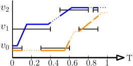
As an example, consider Fig. 2 depicting a g-TAP Instance. Fig. 2b depicts two timing profiles for path : and (recall the times in a timing profile are the times at which the robot reaches the middle of the edges). obtains a reward of and at and , respectively. Thus, while obtains a reward of and at and , respectively. Thus, .
We are finally ready to define our optimization problems:
Problem 1 (OTP).
Let be a path and let be the set of all possible timing profiles over . The Optimal Timing-Profile (OTP) problem calls for computing a timing-profile for whose reward is maximal. Namely, compute s.t.,
Problem 2 (OPTP).
Let be a task assistance graph, a start vertex. Let be the set of paths in starting from and be the set of all possible timing profiles over a given path . The Optimal Path and Timing-Profile (OPTP) problem calls for computing a path and a timing profile whose reward is maximal. Namely, compute s.t.,
4 Solving the OTP Problem (Prob. 1)
At first glance, given a specific path , computing an optimal timing-profile may seem to be a continuous optimization problem as each timestamp can be in the range . However, our first key insight is that we can consider a discrete set of critical times. Roughly speaking, these are the start and end time of intervals while accounting for edges length. This is because there are two conceptual reasons to leave a vertex : either an interval of ended and there is no reason to stay at (as no additional reward will be gained from ), or there is another interval at a successor of we would like to reach further along .
As an example, consider path and the timing profile (which is optimal) from Fig. 2. Here, leaves vertex at time which is exactly the end time of the first interval of . Next, leaves vertex at time which is exactly the time at which the first interval of starts. As we will show, it is enough to consider only critical times to find an optimal timing profile. We Formally define critical times in Sec. 4.1 and show in Sec. 4.2 how they can be used to solve Prob. 1.
4.1 Critical Times
Given two vertices in a path , denotes that lies before in (i.e., that ). Again, when clear, we omit from . Furthermore, we assume that the first and last vertex in contain the intervals and , respectively555These represent the earliest time the first vertex can be left and the latest time the last vertex can be reached, respectively. Adding these intervals does not affect the reward as both interval lengths are zero and are only used to simplify the definitions.. We start by defining the critical times between two vertices in .
Definition 4 (Vertex-pair critical times).
Let be vertices in path such that . The set of vertex-pair critical times consists of two types of times, defined as follows:
-
T1
For any interval , the earliest time to leave after terminates is a type T1 time. Namely, all type T1 times of are
-
T2
For any interval , the latest time needed to leave in order to reach at the start of is a type T2 time. Namely, all type T2 times of are
Each vertex-pair has its own critical times, but the critical times of two pairs sharing a vertex are tightly related. For example, given the path from Fig. 2a, the vertex-pair critical times are:
Notice that bold critical times are identical, and that underlined critical times of are equal to underlined critical times of shifted by . We formalize this relation using the following observations.
Observation 1.
Let be vertices in path such that . is a type T1 in iff is a type T1 in .
Observation 2.
Let be vertices in path such that . is a type T2 in iff is a type T2 in .
Next, we use the notion of vertex-pair critical times to define vertex-critical times which include the times from which might want to leave a vertex.
Definition 5 (Vertex-critical times).
Let be a vertex in path . The set of vertex-critical times for is defined as follows: Let be a vertex-pair critical time for some vertices in s.t. . Then, if
-
,
includes the latest time needed to leave to leave at time .
-
,
includes .
-
,
includes the earliest time we can leave given we left at time .
Formally,
Similar to vertex-pair critical times, vertex-critical times of different vertices are tightly related as well. Following our example from Fig. 2a we have that:
Notice that the critical times are identical up to a constant shift. The following observation formalizes this relation.
Observation 3.
For any vertex , the vertex-critical times are equal to the vertex-critical times of shifted by . Formally,
Lemma 1.
can be computed in time.
Proof (sketch).
Note. Following Obs. 3 we can compute in given .
The next theorem states that an optimal timing-profile can be found by only considering vertex-critical times. To prove the theorem, we show that any optimal timing profile can be transformed to one that contains vertex-critical times only. See Appendix 0.A for details.
Theorem 1.
For any path , there exists an optimal timing profile such that .
4.2 Algorithm
Thm. 1 allows us to present an efficient algorithm that computes the optimal reward (i.e., the reward obtained by following an optimal timing-profile). Specifically, it implies that there exists an optimal timing profile that belongs to . Clearly, one could iterate over all such timing profiles but this is highly-inefficient. Instead, we maintain for each vertex a set of so-called time-reward pairs. Such a time reward-pair at vertex represent a time and a reward that can be obtained by reaching while following a certain timing-profile until time . These time-reward pairs are computed by iterating along the path vertices one at a time while removing time-reward pairs that can’t belong to an optimal timing profile.
Our algorithm (Alg. 1) maintains two time-reward lists representing the list of optional entry and exit times to a certain vertex, respectively. They are initialized to (corresponding to the fact that the initial vertex is entered at time zero with zero reward) and an empty list, respectively (Line 1). The algorithm then proceeds by iterating over the vertices of starting at (Lines 2-9). For each vertex , it iterates over all optional exit times (Lines 4-8) and for each such exit time , computes the best reward obtainable given that vertex must be left at time (Line 5) using the function compute_best_reward (Alg 2). This function simply iterates over all time-reward pairs in Entry. For each entry time-reward pair , it computes the reward obtainable by entering vertex at time and leaving it at time and adds it to the reward obtained prior to entering vertex . After finishing ’s iteration, it sets the exit times of as the entry times of , and sets the exit list to be empty (Line 9). Finally, the algorithm returns the maximal reward it obtained (Line 10).
Input: entry list of critical times: Entry;
vertex: ;
exit time:
Output:
best reward given we leave at time :
Pareto-frontier optimization.
Consider the path from Fig. 2a and recall that . After the first iteration of the algorithm, the time-reward pairs of Exit are:
Now, consider the two pairs and . Here, can be pruned as it leaves the vertex after and its reward is not better. In the general setting, we only need to maintain the Pareto frontier [35] of time-reward pairs. I.e., the set of all time-reward pairs that are not dominated by any other time-reward pair (a time-reward pair dominates a time-reward pair if and or if and . As the time-reward exit pairs are ordered from earliest to latest, we add a pair to Exit only if the reward is greater then the reward of the previous pair (Line 8). Returning to our example, after the first iteration Exit will be pruned down to: .
Correctness & complexity (sketch).
Following Thm. 1, the reward returned by the algorithm corresponds to the reward of an optimal timing-profile. In addition, we can trace back the time-reward pairs in order to find an optimal timing-profile.
Given a path with vertices and a total of intervals we can bound the size of by (Lemma 1). In addition, Entry and Exit are both bounded by . Alg. 2 performs calls of (Line 5). These calls only differ by their value. Since Entry is ordered, the value of only increases. Thus, by computing the value once for the first call, and only substituting the reward for the interval between two following values, we can compute all calls performed in Alg. 2 in time.
To summarize, for each of the vertices, we call Alg. 2 times, and each calls takes time. Thus, the total runtime complexity is .
5 Hardness of the OPTP Problem
We now move on to the OPTP problem and show that it is -hard. Roughly speaking, the hardness of the problem comes from the fact that in the general setting, there may be an exponential number of paths in a graph and in contrast to the shortest-path problem, Bellman’s principle of optimality does not hold.
Theorem 2.
The OPTP problem is -hard.
Sketch.
The proof is by a reduction from the subset-sum problem (SSP) [19]. Recall that the SSP is a decision problem where we are given a set and a target (for simplicity, we assume that but this is a technicality only). The problem calls for deciding whether there exists a set whose sum equals .
Given an SSP instance, we build a corresponding OPTP instance (to be explained shortly) and show that there exists a subset such that iff the optimal reward in our OPTP instance is thus proving the problem is -hard.
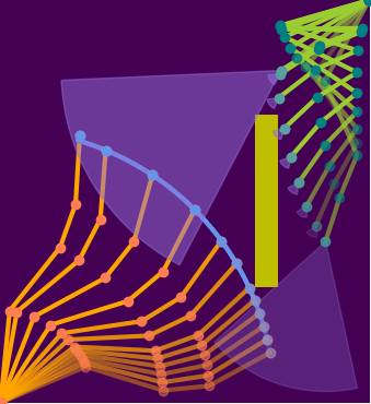
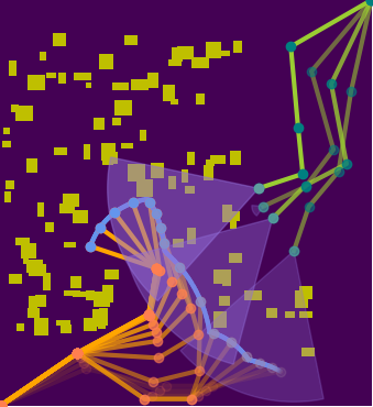
W.l.o.g. assume that are sorted from smallest to largest and set , and . The graph of our OPTP instance depicted in Fig. 3 contains hexagons such that contains vertices . We call and the entry and exit vertices of , and the top of and and the bottom of . Edges and at the top and bottom of have length and , respectively (all other edge lengths are equal to zero). Edge at the top of contains the interval .666Strictly speaking, the interval belongs to the vertices . However, it will be more convenient to consider the interval as belonging to the edge . Finally, the exit of the last hexagon has an edge to a vertex which has a valid interval and has an edge to a vertex whose assistance interval is . Note that here for ease of exposition, time is in the range and not .

Our reduction is based on two key properties of the new OPTP instance:
-
P1
The shortest path to reach is by taking the lower part of each and its length is .
-
P2
Let be a path that passes through . Going through the upper part of adds additional time to reach and results in an additional reward of .
Roughly speaking, the valid interval at forces any path to to leave before time . As the minimal time to reach is (Property ), only has time units to spend on earning rewards from the hexagons. Now, to obtain a reward of , must earn a reward of before reaching . Since the upper part of adds an additional time of and a reward of (Property ), must find a combination of upper parts such that which is the exact solution to the subset-sum problem.
For additional details see Appendix 0.B. ∎
6 Solving the OPTP Problem (Prob. 2)
Given a task assistance graph and a start vertex , we can iterate over all paths starting from , and for each path run the OTP algorithm (Sec. 4). Unfortunately, the search space can be extremely large (Sec. 5) which deems this approach intractable.
To this end, we suggest to apply the Branch and Bound (B&B) framework [6] to our setting. B&B is a general algorithmic technique used to solve optimization problems, particularly combinatorial-optimization problems, by systematically exploring the solution space in a structured manner. Conceptually, B&B divides the solution space into smaller subspaces (branching) and then systematically searches through these subspaces while keeping track of bounds on the optimal solution (bounding). This allows to prune branches of the search tree that are guaranteed not to contain an optimal solution, thereby reducing the size of the search space and improving efficiency.
Thus, we start (Sec. 6.1) by introducing approaches to bound the reward of partial solutions and then continue (Sec. 6.2) to detail our B&B-based algorithm.
6.1 Upper Bound
In the following, we overview how to bound the reward obtainable from (i) any path that starts at the beginning of an interval , (ii) any path that starts at a vertex starting at time and (iii) from a prefix of a path . Here, we give a high-level description regarding how these bounds are computed and refer the reader to Appendix 0.C for additional details.
6.1.1 Bounding the reward obtainable from the beginning of an interval
Let be an interval belonging to vertex . We set and iteratively compute using . As we will see, will be an upper bound on the reward that may be obtained from interval followed by at most subsequent intervals. Note that this indeed holds for and that if the invariant holds for every iteration, then after iterations is an upper bound on the total reward obtainable starting from interval and continuing optimally. To compute , we iterate over all intervals , and bound the reward obtainable assuming the interval after is . This is done by computing , which is the minimal portion of either or in which no reward can obtained when traveling from to . We then bound the reward as . If the bound obtained is greater than , we update it accordingly.
Importantly, stores an upper bound on the reward obtained from interval as well as from future intervals. However, it does not store the time is exited in order to obtain the reward from future intervals. Namely, does not account for the fact that may have been entered at a time . This results in (i) an upper bound on the true reward and (ii) an efficient algorithm whose complexity is cubic in (the number of intervals) and not on the number of critical times which may be exponential in . Note that this process is computed once, before running our B&B-based algorithm and will be used to compute the other bounds required by our algorithm.
Before stating the correctness of , we introduce the following definition:
Definition 6 (Partial reward).
Let be a path, let be a timing-profile and let . We define to be the reward obtained from following the timing-profile during the time interval .
Lemma 2.
Let and be a path and timing-profile, respectively. Let be an interval obtains reward from. Then it holds that .
6.1.2 Bounding the reward obtainable from a vertex starting at time
Let be a vertex and . Denote to be the minimum distance between and in while not accounting for half of the first and last edge (this can be computed using one Dijkstra-like pass over the graph together with some additional processing). Now, consider an interval associated with some vertex . Intuitively, (i) the reward that offers (assuming we start at vertex at time ) cannot be obtained before time and (ii) bounds the reward that can be obtained from . Together, these allow to bound the reward obtainable from at assuming is the next interval. We iterate over all such intervals and set to be the highest reward.
Lemma 3.
Let be a vertex, and . For every path and timing-profile s.t. and that following implies that at time the assistance robot is at vertex , it holds that .
6.1.3 Bounding the reward obtainable given the prefix of a path
Given a path , we wish to compute an upper bound on the reward that can be obtained from any path whose prefix is .
Let be an optimal timing profile for (note that we don’t have access to and but we will address this shortly). Furthermore, let for some be the last interval that obtained reward from before leaving . We bound ’s reward by separating it into two parts: the reward obtained (i) until (the time exits ) and (ii) from .
To bound the reward obtained until (first part), recall that the OTP algorithm keeps track of time-reward pairs representing a time and the best reward that can be obtained until that time at a certain vertex. As is the last interval in that obtains reward from, the reward obtained until can be bounded by the reward obtained until . This is exactly the reward of the pair belonging to the Exit list of vertex which can be computed by running the OTP algorithm on . To bound the reward obtained from (second part) we make use of . Recall that we do not actually have access to but, since obtains reward from it must leave after , which allows us to bound the reward obtainable from by . In addition, since does not obtain any reward between the end of and the time it leaves , we can further tighten our bound to . Combining both parts, can be bounded by .
As we don’t have access to , we can’t know which interval is the last interval obtains reward from. Thus, we must compute this bound for every interval on the path and use the maximal bound obtained to be , our bound on the reward obtainable from the prefix of a path.
Theorem 3.
Let be a path. For any path extending s.t., is its optimal timing profile, it holds that .
Complexity analysis
Given a graph with vertices, edges, and intervals, computing requires computing for every two vertices which can be done in . In addition, each iteration used to compute iterates over all pairs of . Since there are iterations this takes . Thus, computing can be done in . Computing requires iterating once over each interval thus taking time. Finally, given a path with vertices and intervals, computing requires running the OTP algorithm over , and calling once for every interval. Thus, computing can be done in .
6.2 Branch and Bound
We are finally ready to describe our B&B-based algorithm (Alg. 3). This recursive algorithm is given a path (initialized to the start vertex ) and returns the maximal reward obtainable by any path whose prefix is . The algorithm starts by checking if the path can be traversed in time (Line 1). If so, it runs the OTP algorithm to compute ’s optimal reward (Line 3). Subsequently, it checks if any sub-path appended to can improve the currently-stored best reward . This is done by checking if is greater than (Line 4). If this is the case, the algorithm iterates over all adjacent vertices to ’s last vertex (Lines 6-9). For every such vertex the algorithm appends to (Line 7), and performs a recursive call to compute the maximal reward obtainable from any path extending the new path (Line 8). It then updates the maximal reward if needed (Line 9). Finally, it returns the overall maximal reward obtained (Line 10).
Input:
graph: ;
intervals:
path: ; // initialized to
reward: // initialized to
Output:
reward of optimal path and timing profile extending .
Theorem 4.
To improve the algorithm’s runtime, we apply several optimizations:
Cycle pruning.
In contrast to the shortest-path problem, cycles may be beneficial in our setting: They allow to return to previously-visited vertices in future timesteps to make use of multiple intervals associated with the same vertex. However, if a path ends by a cycle which does not provide additional reward, we prune all paths extending this path. This can be done during the algorithm in time using some additional bookkeeping.
Interval splitting.
Let be a path, its optimal timing profile and the last interval obtains reward from before . Let be the vertex belongs to, one can show that counts twice since given the pair from the Exit list of , it upper bounds the reward obtainable from that pair using instead of which allows for to be counted once in the reward and once in . Thus, the smaller the intervals are, the tighter is. Thus, we introduce a parameter . Before running our algorithm, we split every interval of size larger than to a sequence of intervals, each of size less than . Note that (i) as decreases, is tighter but the number of intervals increases which causes a cubic increase in the complexity of the OTP algorithm (see Sec. 4.2) which is used when computing and (ii) this optimization does not affect the solution to the OPTP problem.
Caching & filtering upper bounds.
The computational bottleneck for computing for some path is the frequent calls to (once for every interval in the path). Moreover, for every it holds that . Thus, every time is computed for some and , this value is stored. If, in some subsequent iteration, the algorithms requires to test if the value for some and some , we first test if . Only if this is not the case, we compute and store .
Bounded sub-optimality
We introduce a second hyper-parameter and replace the condition in Line 4 with . This allows to dramatically prune the search space and one can easily show that if and are the rewards obtained with this variation and the optimal reward, respectively, then .
7 Empirical Evaluation
To evaluate our B&B-based algorithm (Alg. 3) we consider the TAP-problem of visual assistance. Specifically, the assistance robot is equipped with a camera that should keep the end-effector of the task robot as-visible as possible.
We consider a simulated environment in which both and are four-link planar manipulators (Fig. 4) as well as the setting depicted in Fig. 1 wherein is a UR5 and is a UR3 [1]. In each scenario, we fix the path of and generate a roadmap using the RRG algorithm [18] containing between to vertices ( was stored with increments of ten vertices). Time intervals in are computed by computing the visible region from each configuration and testing what times the path of intersects this region.
As we optimize our B&B-based algorithm by employing interval splitting and by allowing for bounded sub-optimality, we present our B&B algorithm with two parameters indicating the interval size used for interval splitting and the approximation factor . As we run our algorithm on graphs generated by adding additional vertices and edges, when running the algorithm on a graph with vertices, we use the reward obtained from the previous iteration (on the graph with vertices) to initialize . This allows our algorithm to get close to zero runtimes on iterations where the added vertices can not increase the maximal reward. Consequentially, we present accumulated runtimes.

As baselines to compare with, we suggest the following strawman algorithms: The first, which we term “-discretization” (DD()) discretizes the time into steps of size . It runs a best-first search where nodes are pairs consisting of a vertex and a time with the initial node being (i.e., the start vertex and time ). When expanding a node it can either stay at for time (resulting in the node ) or move to a vertex such that . Note that this algorithm does not guarantee to compute optimal solutions. The second algorithm, which we term DFS-OTP iterates over all possible paths in the graph in a DFS-like approach (stopping when the length of the path exceeds ). When reaching the final vertex of a path, it runs the OTP algorithm on the path. Note that this algorithm is optimal and is in fact identical to the B&B approach with a trivial bound of as it iterates over all paths in the graph.
All algorithms were implemented in C++ and run on a Linux, x86_64 server using an Intel Xeon CPU at 2.10GHz with a timeout of one hour. Code will be made publicly available upon paper acceptance.

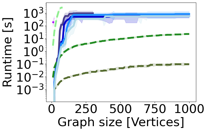
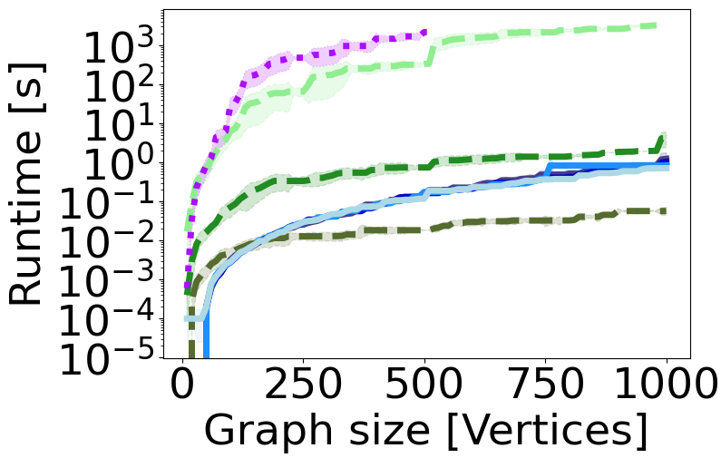
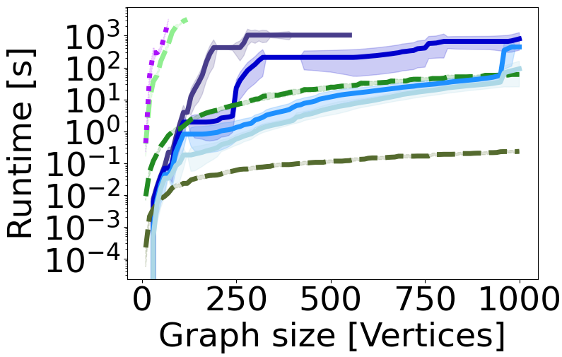
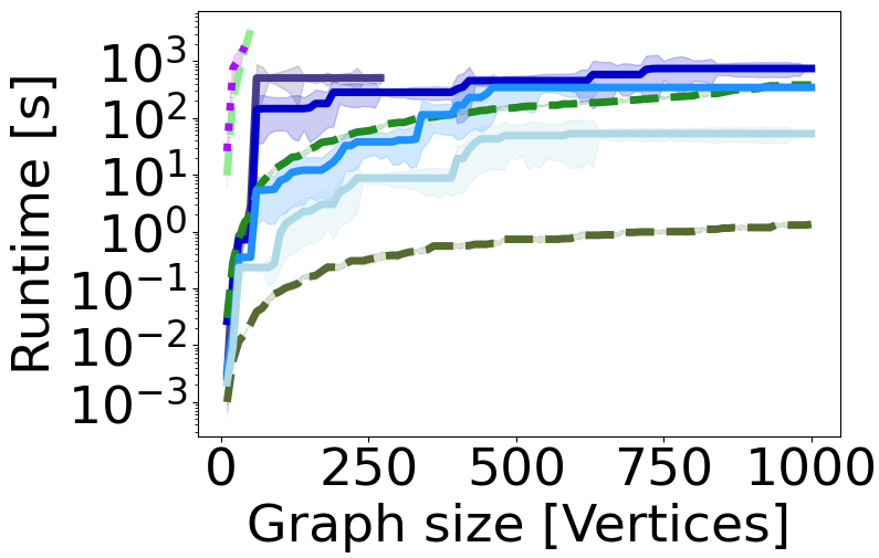
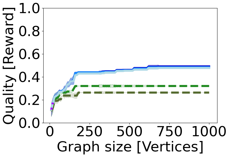
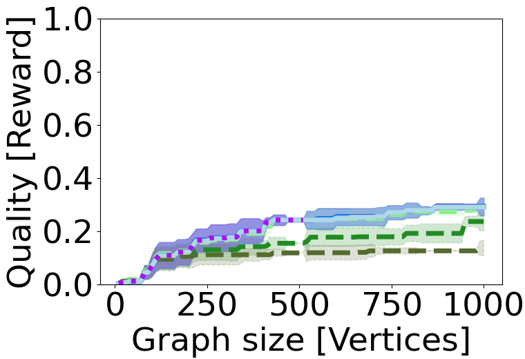
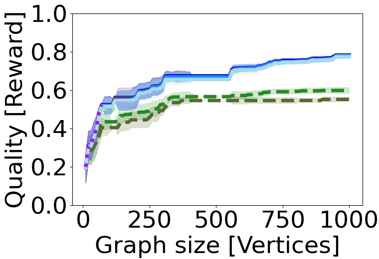
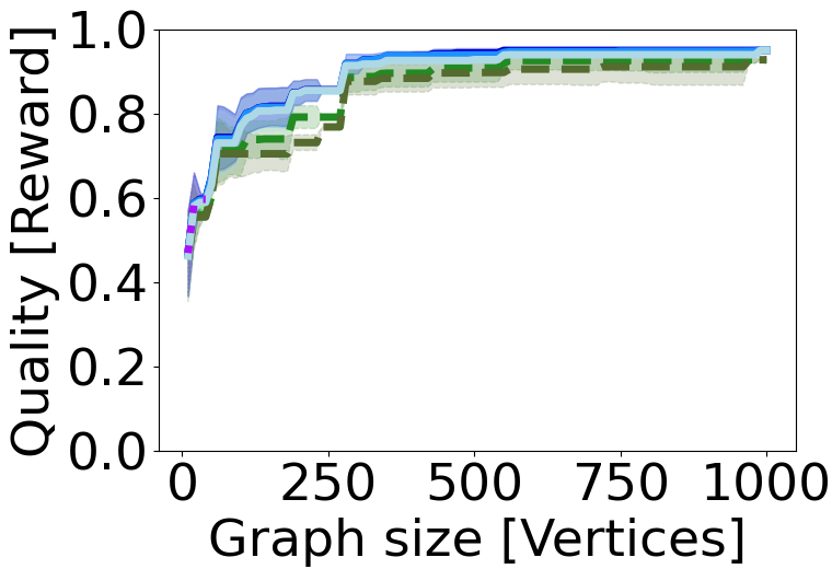
For each one of the four scenarios (three planar manipulators in Fig. 4 and the UR from Fig. 1), we fixed the path of the task robot and generated ten roadmaps. We report in Fig. 5 the average running time and the reward for each algorithm as a function of the number of graph vertices. We present four versions of our B&B algorithm, one with (i.e., an optimal algorithm without interval splitting) and three with the same value for (for interval splitting) but different values of (the approximation factor) as well as DD() with three different values of (smaller values are expected to run longer but obtain higher-quality results) and the DFS-OTP algorithm.
When compared to the baseline optimal algorithm (DFS-OPT), our algorithm allows for an improved runtime by roughly three orders of magnitude for a given graph size and allows to compute solutions for far larger graphs within the allotted planning time of one hour. When compared to the baseline heuristic algorithm (DD()), while being slower, our algorithm obtains higher-quality results by a factor of up to on the three planar scenarios. For the URs, the problem is much easier containing fewer intervals, thus both algorithms produce comparable results (though ours provides guarantees on the solution quality).
As depicted in Fig. 5, and can have a large effect on the performance of our B&B algorithm. Roughly speaking, balances how much time each OTP call takes versus how tight the upper bound is, and reduces the search space size. Recall (Sec. 6), that when computing , the main gap between the real reward obtainable and the upper bound comes from allowing one interval to be counted twice. Thus, smaller intervals result in a smaller gap. However, results in more intervals which increases the runtime of the OTP algorithm. If the approximation factor is larger than the aforementioned gap, it will allow the algorithm to explore only paths whose quality is significantly better that the incumbent solution.
Finally, for a video of UR robots running our algorithm on a scenario similar to Fig. 1, see https://tinyurl.com/yhhurh4n.
8 Future Work
In this work we lay the algorithmic foundation for TAP. Here, we assumed that (A1) the roadmap is provided and that (A2) the path of is known. In future work we wish to relax both assumptions. To relax A1 we intend to build an RRT-like algorithm that reasons about where to sample while taking the task timing into account. To relax A2 we suggest to estimate the path of using some learning algorithm and then iteratively run our B&B algorithm in a model-predictive control (MPC) fashion. Finally, it may be interesting to consider the joint problem of simultaneously planning the path of and .
Acknowledgments
We wish to thank Shaull Almagor for his assistance in proving the hardness of the OTPT problem (Sec. 5) and Dan Elbaz, Ofek Gottlieb for their assistance in the empirical evaluation.
References
- [1] Universal robots, https://www.universal-robots.com
- [2] Almadhoun, R., Taha, T., Seneviratne, L., Dias, J., Cai, G.: A survey on inspecting structures using robotic systems. I. J. Advanced Robotics Systems 13(6) (2016)
- [3] Amuzig, A., Dovrat, D., Keren, S.: Value of assistance for mobile agents. In: IROS. pp. 1594–1600 (2023)
- [4] Bircher, A., Kamel, M., Alexis, K., Oleynikova, H., Siegwart, R.: Receding horizon next-best-view planner for 3d exploration. In: ICRA. pp. 1462–1468. IEEE (2016)
- [5] Chung, T.H., Hollinger, G.A., Isler, V.: Search and pursuit-evasion in mobile robotics - A survey. Auton. Robots 31(4), 299–316 (2011)
- [6] Clausen, J.: Branch and bound algorithms-principles and examples (2003)
- [7] Connolly, C.: The determination of next best views. In: ICRA. vol. 2, pp. 432–435 (1985)
- [8] Dellin, C.M., Srinivasa, S.S.: A unifying formalism for shortest path problems with expensive edge evaluations via lazy best-first search over paths with edge selectors. In: ICAPS. pp. 459–467 (2016)
- [9] Fu, M., Kuntz, A., Salzman, O., Alterovitz, R.: Toward asymptotically-optimal inspection planning via efficient near-optimal graph search. In: RSS (2019)
- [10] Fu, M., Salzman, O., Alterovitz, R.: Computationally-efficient roadmap-based inspection planning via incremental lazy search. In: ICRA. pp. 7449–7456 (2021)
- [11] Galceran, E., Carreras, M.: A survey on coverage path planning for robotics. Robotics and Autonomous systems 61(12), 1258–1276 (2013)
- [12] Geraerts, R.: Camera planning in virtual environments using the corridor map method. In: Motion in Games (MIG). vol. 5884, pp. 194–206 (2009)
- [13] Goemans, O.C., Overmars, M.H.: Automatic generation of camera motion to track a moving guide. In: WAFR. vol. 17, pp. 187–202 (2004)
- [14] Halperin, D., Salzman, O., Sharir, M.: Algorithmic motion planning. In: Csaba D. Toth, Joseph O’Rourke, J.E.G. (ed.) Handbook of Discrete and Computational Geometry, chap. 50, pp. 1307–1338. CRC Press, Inc., 3rd edn. (2017)
- [15] Hart, P.E., Nilsson, N.J., Raphael, B.: A formal basis for the heuristic determination of minimum cost paths. IEEE Transactions on Systems Science and Cybernetics 4(2), 100–107 (1968)
- [16] Hauser, K.: Motion and Path Planning, pp. 1–11. Springer Berlin Heidelberg, Berlin, Heidelberg (2020)
- [17] Howard, R.A.: Information value theory. IEEE Transactions on systems science and cybernetics 2(1), 22–26 (1966)
- [18] Karaman, S., Frazzoli, E.: Sampling-based algorithms for optimal motion planning. Int. J. of Rob. Res. 30(7), 846–894 (2011)
- [19] Kleinberg, J., Tardos, E.: Algorithm design. Pearson Education India (2006)
- [20] Laguna, G.J., Bhattacharya, S.: Path planning with incremental roadmap update for visibility-based target tracking. In: IROS. pp. 1159–1164 (2019)
- [21] LaValle, S.M.: Planning Algorithms. Cambridge University Press (2006)
- [22] LaValle, S.M., González-Baños, H.H., Becker, C., Latombe, J.: Motion strategies for maintaining visibility of a moving target. In: ICRA. pp. 731–736. IEEE (1997)
- [23] Lim, J., Salzman, O., Tsiotras, P.: Class-ordered LPA*: An incremental-search algorithm for weighted colored graphs. In: IROS. pp. 6907–6913 (2021)
- [24] Mandalika, A., Salzman, O., Srinivasa, S.: Lazy receding horizon A* for efficient path planning in graphs with expensive-to-evaluate edges. In: ICAPS. pp. 476–484 (2018)
- [25] Masarwy, M., Goshen, Y., Dovrat, D., Keren, S.: Value of assistance for grasping (2023)
- [26] Nieuwenhuisen, D., Overmars, M.H.: Motion planning for camera movements. In: ICRA. pp. 3870–3876 (2004)
- [27] O’Rourke, J.: Visibility. In: Csaba D. Toth, Joseph O’Rourke, J.E.G. (ed.) Handbook of Discrete and Computational Geometry, chap. 33, pp. 875–896. CRC Press, Inc., 3rd edn. (2017)
- [28] Rakita, D., Mutlu, B., Gleicher, M.: An autonomous dynamic camera method for effective remote teleoperation. In: HRI. pp. 325–333 (2018)
- [29] Rizk, Y., Awad, M., Tunstel, E.W.: Cooperative heterogeneous multi-robot systems: A survey. ACM Computing Surveys (CSUR) 52(2), 1–31 (2019)
- [30] Roberts, M., Leboutet, Q., Prakash, R., Wang, R., Zhang, H., Tang, R., Ferragut, M., Leutenegger, S., Richter, S.R., Koltun, V., Müller, M., Ros, G.: SPEAR: A simulator for photorealistic embodied ai research (2022)
- [31] Robin, C., Lacroix, S.: Multi-robot Target Detection and Tracking: Taxonomy and Survey. Autonomous Robots 40(4), 729–760 (2016)
- [32] Ropero, F., Muñoz, P., R-Moreno, M.D.: TERRA: A path planning algorithm for cooperative ugv–uav exploration. Engineering Applications of Artificial Intelligence 78, 260–272 (2019)
- [33] Russell, S., Wefald, E.: Principles of metareasoning. Artificial intelligence 49(1-3), 361–395 (1991)
- [34] Salzman, O.: Sampling-based robot motion planning. Commun. ACM 62(10), 54–63 (2019)
- [35] Salzman, O., Felner, A., Hernández, C., Zhang, H., Chan, S., Koenig, S.: Heuristic-search approaches for the multi-objective shortest-path problem: Progress and research opportunities. In: ijcai. pp. 6759–6768 (2023)
- [36] Solovey, K.: Complexity of Planning, pp. 1–8. Springer Berlin Heidelberg, Berlin, Heidelberg (2020)
- [37] Zilberstein, S., Lesser, V.: Intelligent information gathering using decision models. CS Department, U. of Massachusetts, Boston, Massachusetts (1996)
Appendix 0.A OPT—Proof of Thm. 1
Theorem 1.
For any path , there exists an optimal timing profile such that .
Proof.
To prove the theorem, we will show that any optimal timing profile can be transformed to one that contains vertex-critical times only.
Let be an optimal timing-profile for , and let be the first index such that . We describe a procedure in which we create another timing-profile such that (i) and that (ii) for all and . Consequently, we can take an optimal timing-profile and run this procedure until an optimal timing-profile exists s.t. (this takes at most iterations).
Our procedure considers two cases: Either there is or there isn’t an interval such that .
Case 1: There is an interval such that .
Here, we consider two different sub-cases corresponding to whether is the last interval that obtains reward from or not.
-
1.1:
is the last interval that obtains reward from.
-
1.2:
is not the last interval that obtains reward from.
Let be an interval such that , and is not the last interval obtains reward from. Let be the next interval obtains reward from after . Note that . Here we distinguish between the setting where and :
-
1.2.1:
.
Here, we will change to leave vertex earlier than . Intuitively, will lose some reward from but, it will earn the same reward back from . First, we show that . Assume by contradiction that , thus . Set for . It holds that:
Which means that which contradicts the optimality of . Thus indeed, .
-
1.2.2:
.
Since obtains reward from , it must hold that . We look at which is the latest time can leave to arrive to at time , and , which is the latest time can leave to be able to leave at time . Set , from Obs. 2 it holds that and from its definition, it holds that . Set for , and . It holds that:
-
1.2.1:
Case 2: There is no interval such that .
Since is not part of an interval, can leave vertex earlier without losing any reward. The two times that are of interest are the earliest time we can leave given we entered at time , and the end time of the last interval of before . By definition, the earliest time can leave vertex is . Since is the earliest time can leave it holds that and since it holds that (Obs. 2). If has at least one interval that ends before starts, we set to be the end time of the last interval ending before . It holds that and from Def. 5 it holds that . If has no such interval we set . We set and . It holds that:
∎
Appendix 0.B OPTP Hardness—Proof of Thm. 2
Theorem 2.
The OPTP problem is -hard.
The proof is by a reduction from the subset-sum problem (SSP) [19]. Recall that the SSP is a decision problem where we are given a set and a target (for simplicity, we assume that but this is a technicality only). The problem calls for deciding whether there exists a set whose sum equals .
Given an SSP instance, we build a corresponding OPTP instance (to be explained shortly) and show that there exists a subset such that iff the optimal reward in our OPTP instance is thus proving the problem is -hard.
W.l.o.g. assume that are sorted from smallest to greatest and set . and . The graph of our OPTP instance depicted in Fig. 3 contains hexagons such that contains vertices . We call and the entry and exit vertices of , and the top of and and the bottom of . Edges and at the top and bottom of have length and , respectively (all other edge lengths are equal to zero). Vertices at the top of contains the interval . Finally, the exit of the last hexagon has an edge to a vertex which has a valid interval and has an edge to a vertex whose assistance interval is . Note that here for ease of exposition, time is in the range and not .

Before we prove Thm. 2, we state several observations and Lemmas.
Observation 4.
Let be a path and a timing profile. If then does not wait at any vertex (except maybe the last one).
Observation 5.
By choosing to go through the lower part of all hexagons (which is the fastest way to reach ) a timing profile can reach u at time .
To see why Obs. 5 holds, let such that , and . Now we have that indeed,
Observation 6.
Let be a path, for every hexagon where goes through the upper part, it adds an additional to the time it takes to reach .
Lemma 4.
Let be a path and a timing profile such that . The reward obtained from choosing the upper part of hexagon is exactly .
Proof.
We start by proving via induction over that can reach hexagon (i.e., reach ) only between (we set and to be ).
Base (): Since starts at the beginning of the first hexagon it reaches at time and indeed .
Step: We assume that the induction hypothesis holds for hexagon and we will prove it for hexagon . can either go through the lower or upper part of hexagon , and following Obs. 4 we know that can’t wait at any vertex of . If goes through the lower part of hexagon , it will reach hexagon between . If goes through the upper part of , it will reach between . Taking a union over both options, we get that will reach between which completes our induction.
Now we can complete the proof of Lemma 4. If traverses the upper part of hexagon , it will reach between . Thus, it will reach between which means must be on the edge between (since never waits at a vertex). In addition thus and since both and have an interval between we get that must obtain a reward of . Since this is the only interval in , obtains a reward of exactly . ∎
Lemma 5.
The maximal reward obtainable for any path before reaching vertex is bounded by .
Proof.
The maximal reward that can be obtained without reaching vertex can be upper bounded by the union of all the intervals that do not belong to . Let be the maximal reward obtainable without reaching , it holds that:
∎
Lemma 6.
The maximal reward obtainable is exactly .
Proof.
Let be an optimal path. From Lemma 5 we know that must reach , and since there is a valid interval on vertex , must reach it before .
Let be the set of items represented by the hexagons at which chose the upper part, formally: . Following Obs. 5, 6 we get that: . From Lemma 4 we get that the reward obtained from choosing the upper part of hexagon is therefore the maximum reward that can be obtained from the hexagons is . We can add the reward we obtain at vertex and get that the maximal reward is . ∎
We are finally ready to prove our theorem.
Proof.
Let be a subset such that . We build our path as follows: for each , if append to the path else append . Finally, append to the end of the path. Next, we build or timing profile by setting , and . We start by showing that we arrive at vertex at time :
Thus, our path and timing profile obtain a reward of 1 in the time interval . We can now analyze the reward obtained during the time interval . From Lemma 4, we get that the reward obtained during the time is equal to:
Thus, the total reward of our path and timing profile is and from Lemma 6 we know it is the maximal reward thus our path and timing profile are optimal.
Now, let be an optimal path and timing profile such that . From Lemma 5 we know that must reach vertex , and since it is possible to reach only before we know that earns a reward of at . Thus, it must earn a reward of until . Let be the set of items represented by the hexagons at which chose the upper part. Formally, . From Lemma 4 we know that the reward obtained from choosing the upper part of hexagon is exactly thus:
which completes our reduction. ∎
Appendix 0.C OPTP Upper Bounds—Additional Details
We start by formally defining . We then describe in detail our algorithm used to compute which was briefly described in Sec 6.1. We then proceed to prove Lemmas 2, 3 and Thm. 3.
Definition 7.
Let be a task-assistance graph. We define to be the minimum distance between and in while not accounting for half of the first and last edge. Namely, if is the set of all paths from to then
if and if no such path exists.
Input: graph ;
intervals:
Output:
upper bound for each interval
Alg. 4 provides the pseudo code to compute . It starts by initializing IntervalSet to be a set containing all intervals, to be the length of interval and to be the number of intervals in (Lines 1-6). It then iterates over all intervals times (Lines 7-14). For each interval , the algorithm iterates over all intervals and bounds the maximal reward obtainable assuming the next interval after is (Lines 11-14). This is done by computing , which is the portion of either or in which no reward can be obtained when traveling from to , and subtracting it from . If the bound obtained is greater then the current , the algorithm updates accordingly (Line 14).
Lemma 2.
Let , be a path and timing-profile. Let be an interval obtains reward from. Then it holds that .
Proof.
Let be the list of intervals obtains reward from ordered from last to first. We will prove the lemma by induction over such that at the end of every iteration , it holds that when .
Base (): Since is the last interval obtains reward from it holds that .
Step: We assume that the induction hypothesis holds for and we will prove for . Let be the vertex belongs to, and the vertex belongs to. can not earn reward for at least time when moving from to . Thus,
From the induction assumption we get that
And after the end of the -th iteration it holds that
Thus, which concludes the proof.
∎
Lemma 3.
Let be a vertex, and . For every path and timing-profile s.t. and that following implies that at time the robot is at vertex , it holds that .
Proof.
Let for some be the first interval obtains reward from after time , and let be the time enters that interval (or if ). Since is the minimal time with no reward between and it holds that . Recall that is the time that must pass since in which can not obtain reward from , then from Lemma 2 it holds that , And from its definition, it holds that , thus, we get that .
∎
Theorem 3.
Let be a path. For any path extending s.t., is its optimal timing profile, it holds that .
Proof.
Let for some be the last interval obtains reward from before leaving . We separate the reward obtained by ’s into two parts: (i) the reward obtained until (the time exits ) and (ii) the reward obtained from .
Since , it holds that is a Vertex-critical time of vertex in . Thus, given the time-reward pair belonging to the Exit list of when running the OTP algorithm on 777 In order for the next part to be correct in the case where , we must consider entering vertex at time which is not considered when computing the pair . To do so, we update the “if” statement (Line 3) in compute_best_reward (Alg. 2) to be: “if ” when running the OTP algorithm for . it holds that , and since we get that .
Additionally, does not obtain reward from to , and it holds that . Thus, from Lemma 3 we get that . Finally:
∎