Double Successive Over-Relaxation Q-Learning with an Extension to Deep Reinforcement Learning

Abstract

Q-learning is a widely used algorithm in reinforcement learning (RL), but its convergence can be slow, especially when the discount factor is close to one. Successive Over-Relaxation (SOR) Q-learning, which introduces a relaxation factor to speed up convergence, addresses this issue but has two major limitations: In the tabular setting, the relaxation parameter depends on transition probability, making it not entirely model-free, and it suffers from overestimation bias. To overcome these limitations, we propose a sample-based, model-free double SOR Q-learning algorithm. Theoretically and empirically, this algorithm is shown to be less biased than SOR Q-learning. Further, in the tabular setting, the convergence analysis under boundedness assumptions on iterates is discussed. The proposed algorithm is extended to large-scale problems using deep RL. Finally, the tabular version of the proposed algorithm is compared using roulette and grid world environments, while the deep RL version is tested on a maximization bias example and OpenAI Gym environments.

I Introduction

Reinforcement learning (RL) is a commonly employed approach for decision-making in a variety of domains, wherein agents learn from their interactions with the environment. The primary goal of RL is to find an optimal policy, which involves solving Bellman’s optimality equation. Depending on the amount of information available, various algorithms are proposed in both dynamic programming and RL to solve Bellman’s optimality equation. When the complete information of the Markov Decision Process (MDP) is available, techniques from dynamic programming, such as value iteration and policy iteration, are utilized to find the optimal value function, thereby, an optimal policy [1]. In cases where the MDP is not fully known (model-free), RL techniques are utilized [2]. Q-learning, introduced by Watkins in 1992, is a fundamental algorithm in RL used to find an optimal policy in model-free environments [3]. Despite its wide application in several areas (see, [4, 5, 6, 7]), Q-learning suffers from slow convergence and over-estimation bias. The drawbacks of Q-learning are well-documented in the literature, and considerable efforts are being made to overcome them (for instance, see [8, 9, 10, 11, 12]).
In 1973, a successive over-relaxation (SOR) technique was proposed by D. Reetz to fasten the convergence of value iteration [13]. This technique involves constructing a modified Bellman equation with a successive over-relaxation parameter. Recently, this technique has been incorporated into Q-learning, resulting in a new algorithm called SOR Q-learning (SORQL)[10]. The underlying deterministic mapping of the SORQL algorithm has been shown to have a contraction factor less than that of the standard Q-Bellman operator [10]. This was achieved by selecting a suitable relaxation factor that depends on the transition probability of a self-loop of an MDP, making the algorithm partially model-free. Furthermore, the theory and our empirical results on benchmark examples have revealed that SOR Q-learning, similar to Q-learning, suffers from overestimation bias. To address these issues, we propose double SOR Q-learning (DSORQL), which combines the idea of double Q-learning [8] with SOR. The advantages of the proposed algorithm are that it is entirely model-free and has been shown, both theoretically and empirically, to have less bias than SORQL. In addition, this work provides the convergence analysis of the proposed algorithm using stochastic approximation (SA) techniques. Recently, the concept of SOR is applied to the well-known speedy Q-learning algorithm [11], leading to the development of a new algorithm called generalized speedy Q-learning, which is discussed in [14]. Further, in [15], the SORQL algorithm has been suitably modified to handle two-player zero-sum games, and consequently, a generalized minimax Q-learning algorithm was proposed. It is also worth noting that a deep RL version of the SOR Q-learning algorithm, similar to the deep Q-network (DQN) [16], is proposed in [17]. Additionally, the application of this deep RL variant of the SOR Q-learning algorithm is discussed for auto-scaling cloud resources [17].
The convergence of several RL algorithms depends on the theory developed in SA [18, 19, 20, 21]. Many of the iterative schemes in the literature assume the boundedness and proceed to show the convergence. For instance, in [15], the convergence of the generalized minimax Q-learning algorithm was shown to converge under the boundedness assumption. In this manuscript, we take the same approach to show the convergence of the proposed algorithms in the tabular setting. Motivated from the work in [16], and [17], wherein the double Q-learning and SOR Q-learning in the tabular version extended to large-scale problems using the function approximation. In this manuscript, we extend the tabular version of the proposed algorithm and present a double successive over-relaxation deep Q-network (DSORDQN). The proposed algorithm is tested on OpenAI gym’s CartPole [22], LunarLander [22] environments, and a maximization example where the state space is in the order of $10^{9}$ [23]. The experiments corroborate the theoretical findings.

The remainder of the paper is organized as follows: In Section II, we discuss the results required for proving the convergence of the proposed algorithms, along with basic notations and terminologies. Section III presents the proposed algorithms, while Section IV addresses the convergence analysis of the proposed algorithms and provides insights into the theoretical understanding of their bias. Numerical experiments are conducted in Section V to demonstrate the effectiveness of the proposed algorithms. Finally, we conclude the manuscript with Section VI.

II Preliminaries

MDP provides a mathematical representation of the underlying control problem and is defined as follows: Let $S$ be the set of finite states and $A$ be the finite set of actions. The transition probability for reaching the state $j$ when the agent takes action $a$ in state $i$ is denoted by $p^{j}_{ia}$. Similarly, let $r^{j}_{ia}$ be a real number denoting the reward the agent receives when an action $a$ is chosen at state $i$, and the agent transitions to state $j$. Finally, the discount factor is $\gamma$, where $0\leq\gamma<1$. A policy $\pi$ is a mapping from $S$ to $\Delta(A)$, where $\Delta(A)$ denotes the set of all probability distributions over $A$. The solution of the Markov decision problem is an optimal policy $\pi^{*}$. The problem of finding an optimal policy $\pi^{*}$ reduces to finding the fixed point of the following operator $U:\mathbb{R}^{|S\times A|}\rightarrow\mathbb{R}^{|S\times A|}$ defined as

$$UQ(i,a)=r(i,a)+\gamma\sum_{j=1}^{|S|}p^{j}_{ia}\mathcal{M}Q(j),$$ (1)

where

$$r(i,a)=\sum_{j=1}^{|S|}p^{j}_{ia}r^{j}_{ia},\quad\text{and}\quad\mathcal{M}Q(j)=\max_{b\in A}Q(j,b).$$

To simplify the equations, we defined the max-operator $\mathcal{M}Q(i)$ as $\max_{a\in A}Q(i,a)$ for $i\in S$. Also, $R_{\max}=\max_{(s,a,s^{\prime})}|r^{s^{\prime}}_{sa}|,\forall(s,a,s^{\prime})\in S\times A\times S$. These notations will be used throughout the manuscript as necessary. Note that $U$ is a contraction operator with $\gamma$ as the contraction factor, and $Q^{*}$ serves as the optimal action-value function of the operator $U$. Moreover, one can obtain an optimal policy $\pi^{*}$ from the $Q^{*}$, using the relation $\pi^{*}(i)\in\text{arg}\,\mathcal{M}Q^{*}(i),\;\forall i\in S.$ Q-learning algorithm is a SA version of Bellman’s operator $U$. Given a sample $\{i,a,j,r^{j}_{ia}\}$, current estimate $Q_{n}(i,a)$, and a suitable step-size $\beta_{n}(i,a)$, the update rule of Q-learning is as follows

$$Q_{n+1}(i,a)=Q_{n}(i,a)+\beta_{n}(i,a)(r^{j}_{ia}+\gamma\,\mathcal{M}Q_{n}(j)-Q_{n}(i,a)).$$

Under suitable assumptions, the above iterative scheme is shown to converge to the fixed point of $U$ with probability one (w.p.1) [3, 18, 19]. Recently, in [10], a new Q-learning algorithm known as successive over-relaxation Q-learning (SORQL) is proposed to fasten the convergence of Q-learning. More specifically, a modified Bellman’s operator is obtained using the successive over-relaxation technique. In other words, instead of finding the fixed point of $U$, the fixed point of the modified Bellman’s operator $U_{w}:\mathbb{R}^{|S\times A|}\rightarrow\mathbb{R}^{|S\times A|}$ is evaluated and is defined as

$$(U_{w}Q)(i,a)$$

$$=w\bigg{(}r(i,a)+\gamma\sum_{j=1}^{|S|}p^{j}_{ia}\mathcal{M}Q(j)\bigg{)}+(1-w)\mathcal{M}Q(i),$$

where $0<w\leq w^{*}$, and $w^{*}=\min\limits_{i,a}\left\{\frac{1}{1-\gamma p^{i}_{ia}}\right\}.$
In [10], it was shown that $U_{w}$ is $1-w+w\gamma$-contractive. Moreover, from Lemma 4, in [10] for $1\leq w\leq w^{*}$ the contraction factor of the operator $U_{w}$ satisfy $1-w+\gamma w\leq\gamma$. Further, it was shown that

$$\mathcal{M}Q^{*}_{w}(i)=\mathcal{M}Q^{*}(i),\,\forall i\in S,$$ (2)

where $Q^{*}$ and $Q^{*}_{w}$ are the fixed points of $U$ and $U_{w}$, respectively. Under suitable assumptions, it was proved that the SORQL algorithm given by the update rule

$$Q_{n+1}(i,a)$$

$$=(1-\beta_{n}(i,a)Q_{n}(i,a)+\beta_{n}(i,a)\Big{[}w\Big{(}r^{j}_{ia}+\gamma\,\mathcal{M}Q_{n}(j)\Big{)}$$

$$\hskip 56.9055pt+(1-w)\mathcal{M}Q_{n}(i)\Big{]},$$ (3)

where $0<w\leq w^{*}$, and $0\leq\beta_{n}(i,a)\leq 1$ converges to the fixed point of $U_{w}$ w.p.1 [10]. Note that the successive relaxation factor in the above equation depends on the transition probability, which makes it not entirely model-free. Owing to this and the natural concerns regarding the over-estimation of SORQL. This manuscript proposes a model-free variant of the SORQL algorithm and a model-free double SOR Q-learning algorithm. To prove the convergence of the proposed algorithms in the tabular setting, the following result from [21] will be useful, and we conclude this section by stating it here as lemma.

Lemma 1.

(Lemma 1, in [21]) Let a random process $\left(\Phi_{n},J_{n},\beta_{n}\right),$ $n\geq 0$, where $\Phi_{n},J_{n},\beta_{n}:X\rightarrow\mathbb{R}$ satisfy the following relation:
$\Phi_{n+1}(x)=(1-\beta_{n}(x))\Phi_{n}(x)+\beta_{n}(x)J_{n}(x),\;\text{where}\hskip 5.69046ptx\in X.$ Suppose $\mathcal{G}_{n}$ is an increasing sequence of $\sigma$-fields with $\beta_{0}$, $\Phi_{0}$ are $\mathcal{G}_{0}$ measurable and $\beta_{n}$, $\Phi_{n}$, $J_{n-1}$ are $\mathcal{G}_{n}$ measurable for $n\geq 1$. Then $\Phi_{n}$ $\rightarrow$ $0$ w.p.1 as $n$ $\rightarrow$ $\infty$, under the following conditions: (1) $X$ is a finite set. (2) Step-size satisfy, $0\leq\beta_{n}(x)\leq 1$, $\sum_{n=1}^{\infty}\beta_{n}(x)=\infty$, $\sum_{n=1}^{\infty}\beta^{2}_{n}(x)<\infty$ $w.p.1.$ (3) $\|E[J_{n}|\mathcal{G}_{n}]\|\leq K\|\Phi_{n}\|+\delta_{n}$, where $K\in[0,1)$ and $\delta_{n}$ $\rightarrow$ $0$ $w.p.1$. (4) $Var[J_{n}(x)|\mathcal{G}_{n}]\leq C(1+\|\Phi_{n}\|)^{2}$, where $C$ is some constant.

III Proposed Algorithm

In this section, we first discuss the tabular version of the proposed algorithms, followed by a discussion of the deep RL version.

III-A Tabular version:

This subsection presents the model-free variants of the algorithm SOR Q-learning and double SOR Q-learning. As previously mentioned, the successive relaxation factor $w$ is dependent on $p^{i}_{ia}$, which is generally unknown. To remove this dependency on the transition probability of a self-loop, the following scheme is proposed: For any $i,j\in S$ and $a\in A$, let $Y_{n}[i][j][a]$ denote the number of times the states $i,j$ and action $a$ are visited till $n^{th}$ iteration. Further, we assume $Y_{0}[i][j][a]=0,\,\forall i,j,a\in S\times S\times A$, and define

$$\widetilde{P}^{j}_{ia}=\dfrac{Y_{n}[i][j][a]}{n},\quad\forall n\geq 1.$$

Using the strong law of large numbers $\widetilde{P}^{j}_{ia}\rightarrow p^{j}_{ia},\,\forall\,i,j,a$ as $n\rightarrow\infty$, w.p.1. Now for $w_{0}\in[1,\frac{1}{1-\gamma}]$, and $\alpha(n)$ satisfying step-size condition (2) in Lemma 1, we consider the following iterative scheme

$$w_{n+1}=w_{n}+\alpha(n)\bigg{(}\dfrac{1}{1-\gamma\min\limits_{i,a}\widetilde{P}^{j}_{ia}}-w_{n}\bigg{)},\quad n\geq 1.$$ (4)

We rewrite the above iterative scheme as follows

$$w_{n+1}=w_{n}+\alpha(n)(f(w_{n})+\epsilon_{n}),\quad n\geq 1,$$ (5)

where

$$f(w_{n})=\dfrac{1}{1-\gamma\min\limits_{i,a}p^{j}_{ia}}-w_{n},\;\epsilon_{n}=\dfrac{1}{1-\gamma\min\limits_{i,a}\widetilde{P}^{j}_{ia}}-w^{*}.$$

Since $\widetilde{P}^{j}_{ia}\rightarrow p^{j}_{ia}$ w.p.1, this implies $\epsilon_{n}\rightarrow 0$ as $n\rightarrow\infty$ w.p.1. Note that for any $w_{1},w_{2}\in\mathbb{R}$

$$|f(w_{1})-f(w_{2})|\leq|w_{1}-w_{2}|.$$

The iterate $\{w_{n}\}$ in (4) track the the ODE, $\dot{w}=w^{*}-w$ [[20], Section 2.2]. Let $f_{\infty}(w)=\lim_{r\rightarrow\infty}\frac{f(rw)}{r}$. The function $f_{\infty}(w)$ exist and is equal to $-w$. Further, the origin and $w^{*}$ is the unique globally asymptotically stable equilibrium for the ODE $\dot{w}=f_{\infty}(w)=-w$ and $\dot{w}=w^{*}-w$, respectively.
As a result of the above observations and [20], one can obtain the following theorem

Theorem 1.

The iterative scheme defined in (4), satisfy $\sup_{n}\,\|w_{n}\|<\infty$ w.p.1. Further, $w_{n}$ $\rightarrow$ $w^{*}$ w.p.1 as $n\rightarrow\infty$.

Proof.

The proof is a consequence of Theorem 7 in Chapter 3, and Theorem 2 - Corollary 4 in Chapter 2 [20]. ∎

Note 1.

Throughout this manuscript, the sequence $w_{n}$ is assumed to be updated using (4).

Remark 1.

The model-free SORQL (MF-SORQL) algorithm is nothing but Algorithm 1 in [10], with $w$ replaced by $w_{n}$.

Algorithm 1 Model-Free Double SOR Q-Learning (MF-DSORQL)

1:$Q^{A}_{0}$, $Q^{B}_{0}$; $\gamma$, $\beta_{n}$, $w_{n}$, $N$, policy $\mu$ producing every $S\times A$ pairs indefinitely.

2:for $n=0,1,\cdots,N-1$ do

3:     Choose $a$ at $i_{n}$ according to $\mu$

4:     Observe samples $i^{\prime}_{n}$ and $r^{\prime}_{n}$

5:     Update $Q^{A}_{n+1}$ or $Q^{B}_{n+1}$ with equal probability

6:     if $Q^{A}_{n+1}$ is updated then

7:         $b^{*}=\arg\max_{b}Q^{A}_{n}(i^{\prime}_{n},b)$

8:         $c^{*}=\arg\max_{c}Q^{A}_{n}(i_{n},c)$

9:         $Q^{A}_{n+1}(i_{n},a_{n})=(1-\beta_{n}(i_{n},a_{n}))Q^{A}_{n}(i_{n},a_{n})+\beta_{n}(i_{n},a_{n})\big{(}w_{n}(r^{\prime}_{n}+\gamma Q^{B}_{n}(i^{\prime}_{n},b^{*}))+(1-w_{n})Q^{B}_{n}(i_{n},c^{*})\big{)}$

10:     else

11:         $d^{*}=\arg\max_{d}Q^{A}_{n}(i^{\prime}_{n},d)$

12:         $e^{*}=\arg\max_{e}Q^{A}_{n}(i_{n},e)$

13:         $Q^{B}_{n+1}(i_{n},a_{n})=(1-\beta_{n}(i_{n},a_{n}))Q^{B}_{n}(i_{n},a_{n})+\beta_{n}(i_{n},a_{n})\big{(}w_{n}(r^{\prime}_{n}+\gamma Q^{A}_{n}(i^{\prime}_{n},d^{*}))+(1-w_{n})Q^{A}_{n}(i_{n},e^{*})\big{)}$  

14:     end if

15:     $i_{n+1}=i^{\prime}_{n}$

16:end for

17:return $Q_{N-1}$

Remark 2.

If the sequence $\{w_{n}\}_{n\geq 0}$ in Algorithm 1 is a constant sequence, with $w$ as the constant and $0<w\leq w^{*}$, we refer to this algorithm as double SOR Q-learning (DSORQL). Therefore, given the samples $\{i,a,j,r^{j}_{ia}\}$ the update rule for the DSORQL is as follows:
With probability $0.5$ update $\widetilde{Q}^{A}$:

$$\widetilde{Q}^{A}_{n+1}(i,a) =(1-\beta_{n})\widetilde{Q}^{A}_{n}(i,a)$$

$$\;+\beta_{n}\Big{[}w\big{(}r^{j}_{ia}+\gamma\widetilde{Q}^{B}_{n}(j,b^{*})\big{)}+(1-w)\big{(}\widetilde{Q}^{B}_{n}(i,c^{*})\big{)}\Big{]}$$

else update $\widetilde{Q}^{B}$:

$$\widetilde{Q}^{B}_{n+1}(i,a) =(1-\beta_{n})\widetilde{Q}^{B}_{n}(i,a)$$

$$\;+\beta_{n}\Big{[}w\big{(}r^{j}_{ia}+\gamma\widetilde{Q}^{A}_{n}(j,d^{*})\big{)}+(1-w)\big{(}\widetilde{Q}^{A}_{n}(i,e^{*})\big{)}\Big{]},$$

where $\beta_{n}=\beta_{n}(i,a)$, and $b^{*},c^{*},d^{*}$, $e^{*}$ are as in Alg. 1.

Note 2.

The SORQL algorithm discussed in [10] and the DSORQL algorithm mentioned in Remark 2 become model-free when $|S|=1$. Therefore, these algorithms can be implemented directly in single-state MDPs, wherein $w$ will be known and satisfy $0<w\leq w^{*}=\frac{1}{1-\gamma}$.

III-B Deep RL version:

In [24], the authors highlight the issue of overestimation in DQN on large-scale deterministic problems. They introduce double DQN (DDQN), a modified version of the DQN algorithm that effectively reduces the over-estimation.
The proposed double SOR deep Q-network (DSORDQN) is a deep RL version of the tabular DSORQL. DSORDQN utilizes the technique of SOR method with DDQN. Specifically, similar to DDQN we use online Q-network $Q(S,a;\theta)$ for selecting the actions, and the target Q-network $Q(S,a;\theta^{\prime})$, to evaluate the actions. The gradient descent will be performed on the following loss function: $L(\theta_{i})=E\big{[}(y_{j}-Q(s,a;\theta_{i}))^{2}\big{]},$ where $y_{j}=w(r(i_{j},a_{j})+\gamma Q(i_{j+1},\operatorname*{arg\,max}_{b}Q(i_{j+1},b;\theta_{i});\theta^{\prime}_{i})+(1-w)Q(i_{j},\operatorname*{arg\,max}_{e}Q(i_{j},e;\theta_{i});\theta^{\prime}_{i})$ for sample $(i_{j},a_{j},r(i_{j},a_{j}),i_{j+1})$ from the replay buffer with $w>1$. Interestingly, the advantages of DDQN and SORDQN transfer to the proposed DSORDQN algorithm, resulting in more stable and reliable learning at scale.

IV Theoretical Analysis

At first, we discuss the convergence of model-free SOR Q-learning (Remark 1) under the following assumption: (A1): $\|Q_{n}\|\leq B<\infty$, $\forall n\geq 0$.

Theorem 2.

Suppose (A1) holds. Given an MDP defined as in Section II, and $w_{n}$ as in (4). Let every state-action pair be sampled indefinitely. Then, for sample $\{i,a,j,r^{j}_{ia}\}$ the update rule of model-free SOR Q-learning algorithm given by:

$$Q_{n+1}(i,a) =(1-\beta_{n}(i,a))Q_{n}(i,a)$$ (6)

$$\quad+\beta_{n}(i,a)\left[w_{n}\left(r^{j}_{ia}+\gamma\mathcal{M}Q_{n}(j)\right)\right.$$

$$\quad\left.+(1-w_{n})\left(\mathcal{M}Q_{n}(i)\right)\right]$$

converges w.p.1 to the fixed point of $U_{w^{*}}$, where $\sum_{n}\beta_{n}(i,a)=\infty,\;\sum_{n}\beta^{2}_{n}(i,a)<\infty,$ and $0\leq\beta_{n}(i,a)\leq 1$.

Proof.

The correspondence to Lemma 1 follows from associating $X$ with the set of state-action pairs $(i,a)$, $\beta_{n}(x)$ with $\beta_{n}(i,a)$, and $\Phi_{n}(i,a)$ with $Q_{n}(i,a)-Q^{*}_{w^{*}}(i,a)$, where $Q^{*}_{w^{*}}$ is the fixed point of $U_{w^{*}}$. Let the filtration for this process be defined by, $\mathcal{G}_{n}=\{Q_{0},i_{j},a_{j},\beta_{j},w_{j},\forall j\leq n,n\geq 0\}$. Note that $\mathcal{G}_{n}\subseteq\mathcal{G}_{n+1},\forall n\geq 0.$ The iteration of model-free SORQL is rewritten as follows:

$$\Phi_{n+1}(i_{n},a_{n}) =(1-\beta_{n}(i_{n},a_{n}))\Phi_{n}(i_{n},a_{n})$$

$$\quad+\beta_{n}(i_{n},a_{n})\left[w_{n}\left(r^{i_{n+1}}_{i_{n}a_{n}}+\gamma\mathcal{M}Q_{n}(i_{n+1})\right)\right.$$

$$\quad\left.+(1-w_{n})\left(\mathcal{M}Q_{n}(i_{n})\right)-Q^{*}_{w^{*}}(i_{n},a_{n})\right].$$

Without loss of generality, let $J_{n}(i,a)=w_{n}(r^{j}_{ia}+\gamma\,\mathcal{M}Q_{n}(j))+(1-w_{n})(\mathcal{M}Q_{n}(i))-Q^{*}_{w^{*}}(i,a).$ Also $\beta_{0}$, $\Phi_{0}$ is $\mathcal{G}_{0}$ measurable and $\beta_{n}$, $\Phi_{n}$, $J_{n-1}$ are $\mathcal{G}_{n}$ measurable for $n\geq 1$. Define $J^{Q}_{n}=w^{*}(r^{j}_{ia}+\gamma\mathcal{M}Q_{n}(j))+(1-w^{*})(\mathcal{M}Q_{n}(i))$. We now consider,

$$\left|E[J_{n}(i,a)\mid\mathcal{G}_{n}]\right|$$

$$=\left|E\left[J_{n}(i,a)+J^{Q}_{n}-J^{Q}_{n}+Q^{*}_{w^{*}}(i,a)-Q^{*}_{w^{*}}(i,a)\mid\mathcal{G}_{n}\right]\right|$$

$$\leq\big{|}\sum_{j=1}^{|S|}p^{j}_{ia}\left(w^{*}\left(r^{j}_{ia}+\gamma\mathcal{M}Q_{n}(j)\right)\right.$$

$$\quad\left.+(1-w^{*})\mathcal{M}Q_{n}(i)\right)-Q^{*}_{w^{*}}(i,a)\big{|}$$

$$\quad+\left|w_{n}-w^{*}\right|\left|E\left[r^{j}_{ia}+\gamma\mathcal{M}Q_{n}(j)+\mathcal{M}Q_{n}(i)\mid\mathcal{G}_{n}\right]\right|$$

$$\leq\left|U_{w^{*}}Q_{n}(i,a)-U_{w^{*}}Q^{*}_{w^{*}}(i,a)\right|$$

$$\quad+\left|w_{n}-w^{*}\right|\left(R_{\max}+2\|Q_{n}\|\right)$$

$$\leq(1-w^{*}+w^{*}\gamma)\|\Phi_{n}\|+\delta_{n},$$

where $\delta_{n}=|w_{n}-w^{*}|(R_{\max}+2\|Q_{n}\|)$. From Theorem 1 and (A1), $\delta_{n}$ $\rightarrow$ $0$ as $n\rightarrow\infty$. Therefore, condition $(3)$ of Lemma 1 holds. Now we verify the condition (4) of Lemma 1,

$$Var[J_{n}(i,a)|\mathcal{G}_{n}]$$

$$=E\left[\left(J_{n}(i,a)-E[J_{n}(i,a)|\mathcal{G}_{n}]\right)^{2}|\mathcal{G}_{n}\right]$$

$$\leq E\left[\left(w_{n}(r^{j}_{ia}+\gamma\mathcal{M}Q_{n}(j))+(1-w_{n})(\mathcal{M}Q_{n}(i))\right)^{2}|\mathcal{G}_{n}\right]$$

$$\leq 3\left(\kappa R_{\max}^{2}+\kappa\gamma^{2}\|Q_{n}\|^{2}+\kappa_{1}\|Q_{n}\|^{2}\right)$$

$$\leq 3\left(\kappa R_{\max}^{2}+2(\kappa\gamma^{2}+\kappa_{1})(\|\Phi_{n}\|^{2}+\|Q^{*}_{w^{*}}\|^{2})\right)$$

$$\leq 3\left(\kappa R_{\max}^{2}+2(\kappa\gamma^{2}+\kappa_{1})\|\Phi_{n}\|^{2}+2(\kappa\gamma^{2}+\kappa_{1})\|Q^{*}_{w^{*}}\|^{2}\right)$$

$$\leq\left(3\kappa R_{\max}^{2}+6(\kappa\gamma^{2}+\kappa_{1})\|Q^{*}_{w^{*}}\|^{2}+6(\kappa\gamma^{2}+\kappa_{1})\|\Phi_{n}\|^{2}\right)$$

$$\leq C(1+\|\Phi_{n}\|^{2})\leq C(1+\|\Phi_{n}\|)^{2},$$

where $C=\max\{3\kappa R_{\max}^{2}+6(\kappa\gamma^{2}+\kappa_{1})\|Q^{*}_{w^{*}}\|^{2},6(\kappa\gamma^{2}+\kappa_{1})\}$, $w_{n}^{2}<\kappa$ and $(1-w_{n})^{2}<\kappa_{1}$. Therefore, all the conditions of Lemma 1 holds and hence $\Phi_{n}\rightarrow 0$ w.p.1, therefore, $Q_{n}\rightarrow Q^{*}_{w^{*}}$ w.p.1. ∎

Before going to discuss the convergence of the double SOR Q-learning algorithm mentioned in Remark 2. A characterization result for the dynamics of $V^{BA}_{n}(i,a):=\widetilde{Q}^{B}_{n}(i,a)-\widetilde{Q}^{A}_{n}(i,a)$ will be presented.

Lemma 2.

Consider the updates $\widetilde{Q}^{A}_{n}$ and $\widetilde{Q}^{B}_{n}$ as in Remark 2. Then $E[V^{BA}_{n}(i,a)|\mathcal{G}_{n}]$ converges to zero w.p.1 as $n\rightarrow\infty$.

Proof.

Suppose $V^{BA}_{n+1}(i,a):=\widetilde{Q}^{B}_{n+1}(i,a)-\widetilde{Q}^{A}_{n+1}(i,a)$. Then Remark 2 indicates that at each iteration, either $\widetilde{Q}^{A}$ or $\widetilde{Q}^{B}$ is updated with equal probability. If $\widetilde{Q}^{A}$ is getting updated at $(n+1)^{th}$ iteration, then we have

$$V^{BA}_{n+1}(i,a)$$

$$=\widetilde{Q}^{B}_{n}(i,a)-\big{(}(1-\beta_{n})\widetilde{Q}^{A}_{n}(i,a)+\beta_{n}(w(r^{j}_{ia}+\gamma\widetilde{Q}^{B}_{n}(j,b^{*}))$$

$$\hskip 28.45274pt+(1-w)\widetilde{Q}^{B}_{n}(i,c^{*}))\big{)}$$

$$\stackrel{{\scriptstyle\scriptscriptstyle(\mkern-1.5mui\mkern-1.5mu)}}{{=}}(1-\beta_{n})V^{BA}_{n}(i,a)+\beta_{n}\big{(}\widetilde{Q}^{B}_{n}(i,a)-w(r^{j}_{ia}+\gamma\widetilde{Q}^{B}_{n}(j,b^{*}))$$

$$\hskip 28.45274pt-(1-w)\widetilde{Q}^{B}_{n}(i,c^{*}))\big{)}.$$

Similarly if $\widetilde{Q}^{B}$ is getting updated at $(n+1)^{th}$ iteration, then

$$V^{BA}_{n+1}(i,a) =(1-\beta_{n})\widetilde{Q}^{B}_{n}(i,a)+\beta_{n}\big{(}w(r^{j}_{ia}+\gamma\widetilde{Q}^{A}_{n}(j,d^{*}))$$

$$\hskip 28.45274pt+(1-w)\widetilde{Q}^{A}_{n}(i,e^{*})\big{)}-\widetilde{Q}^{A}_{n}(i,a)$$

$$\stackrel{{\scriptstyle\scriptscriptstyle(\mkern-1.5muii\mkern-1.5mu)}}{{=}}(1-\beta_{n})V^{BA}_{n}(i,a)+\beta_{n}\big{(}w(r^{j}_{ia}+\gamma\widetilde{Q}^{A}_{n}(j,d^{*}))$$

$$\hskip 28.45274pt+(1-w)\widetilde{Q}^{A}_{n}(i,e^{*}))-\widetilde{Q}^{A}_{n}(i,a)\big{)}.$$

Combining $(i)$ and $(ii)$, we have

$$V^{BA}_{n+1}(i,a) =(1-\beta_{n})V^{BA}_{n}(i,a)+\beta_{n}J^{A}_{n}(i,a),$$

$$V^{BA}_{n+1}(i,a) =(1-\beta_{n})V^{BA}_{n}(i,a)+\beta_{n}J^{B}_{n}(i,a),$$

where

$$J^{A}_{n}(i,a)=\widetilde{Q}^{B}_{n}(i,a)-w(r^{j}_{ia}+\gamma\widetilde{Q}^{B}_{n}(j,b^{*}))-(1-w)\widetilde{Q}^{B}_{n}(i,c^{*}),$$

$$J^{B}_{n}(i,a)=w(r^{j}_{ia}+\gamma\widetilde{Q}^{A}_{n}(j,d^{*}))+(1-w)\widetilde{Q}^{A}_{n}(i,e^{*}))-\widetilde{Q}^{A}_{n}(i,a).$$

Therefore,

$$E[V^{BA}_{n+1}(i,a)|\mathcal{G}_{n}]$$

$$=(1-\dfrac{\beta_{n}}{2})E[V^{BA}_{n}(i,a)|\mathcal{G}_{n}]+\dfrac{\beta_{n}}{2}E[w\gamma(\widetilde{Q}^{A}_{n}(j,d^{*})$$

$$\hskip 28.45274pt-\widetilde{Q}^{B}_{n}(j,b^{*}))+(1-w)(\widetilde{Q}^{A}_{n}(i,e^{*})-\widetilde{Q}^{B}_{n}(i,c^{*}))|\mathcal{G}_{n}].$$

Let $\dfrac{\beta_{n}}{2}=\zeta_{n}$. Then, the above equation is reduced to

$$E[V^{BA}_{n+1}(i,a)|\mathcal{G}_{n}] =(1-\zeta_{n})E[V^{BA}_{n}(i,a)|\mathcal{G}_{n}]+\zeta_{n}J^{BA}_{n}(i,a),$$ (7)

where

$$J^{BA}_{n}(i,a) =E[w\gamma(\widetilde{Q}^{A}_{n}(j,d^{*})-\widetilde{Q}^{B}_{n}(j,b^{*}))$$

$$+(1-w)(\widetilde{Q}^{A}_{n}(i,e^{*})-\widetilde{Q}^{B}_{n}(i,c^{*}))|\mathcal{G}_{n}].$$

Now for the above recursive Equation (7), we verify the following conditions : (a) $\|E[J^{BA}_{n}|\mathcal{G}_{n}]\|\leq(1-w+w\gamma)\|V^{BA}_{n}\|$ and (b) $Var[J^{BA}_{n}|\mathcal{G}_{n}]\leq C(1+\|V^{BA}_{n}\|)^{2}$. Note that once we verify (a) and (b), then from Lemma 1, we can conclude that the iterative scheme obtained in (7) converges to zero w.p.1. Using the law of total expectation, the condition (b) is trivially satisfied. We now consider,

$$|E[J^{BA}_{n}(i,a)|\mathcal{G}_{n}]|$$

$$=|E[w\gamma(\widetilde{Q}^{A}_{n}(j,d^{*})-\widetilde{Q}^{B}_{n}(j,b^{*}))$$

$$\hskip 28.45274pt+(1-w)(\widetilde{Q}^{A}_{n}(i,e^{*})-\widetilde{Q}^{B}_{n}(i,c^{*}))|\mathcal{G}_{n}]|$$

$$=|\sum_{j=1}^{|S|}p^{j}_{ia}w\gamma(\widetilde{Q}^{A}_{n}(j,d^{*})-\widetilde{Q}^{B}_{n}(j,b^{*}))$$

$$\hskip 28.45274pt+(1-w)(\widetilde{Q}^{A}_{n}(i,e^{*})-\widetilde{Q}^{B}_{n}(i,c^{*}))|$$

$$=|w\gamma\sum_{j=1,j\neq i}^{|S|}p^{j}_{ia}(\widetilde{Q}^{A}_{n}(j,d^{*})-\widetilde{Q}^{B}_{n}(j,b^{*}))$$

$$\hskip 28.45274pt+(w\gamma p^{i}_{ia}+(1-w))(\widetilde{Q}^{A}_{n}(i,e^{*})-\widetilde{Q}^{B}_{n}(i,c^{*}))|$$

$$\stackrel{{\scriptstyle\scriptscriptstyle(\mkern-1.5mui\mkern-1.5mu)}}{{\leq}}w\gamma\sum_{j=1,j\neq i}^{|S|}p^{j}_{ia}|\widetilde{Q}^{A}_{n}(j,d^{*})-\widetilde{Q}^{B}_{n}(j,b^{*})|$$

$$\hskip 28.45274pt+(w\gamma p^{i}_{ia}+(1-w))|(\widetilde{Q}^{A}_{n}(i,e^{*})-\widetilde{Q}^{B}_{n}(i,c^{*}))|.$$

Since $0<w\leq w^{*}$, this implies $(1-w+w\gamma p^{i}_{ia})\geq 0$. Therefore $(i)$ holds in the above equation. Clearly, at each step of the iteration either $\widetilde{Q}^{A}_{n}(j,d^{*})\geq\widetilde{Q}^{B}_{n}(j,b^{*})$ or $\widetilde{Q}^{B}_{n}(j,b^{*})>\widetilde{Q}^{A}_{n}(j,d^{*})$. Suppose $\widetilde{Q}^{A}_{n}(j,d^{*})\geq\widetilde{Q}^{B}_{n}(j,b^{*})$, then

$$|\widetilde{Q}^{A}_{n}(j,d^{*})-\widetilde{Q}^{B}_{n}(j,b^{*})|$$

$$=\widetilde{Q}^{A}_{n}(j,d^{*})-\widetilde{Q}^{B}_{n}(j,b^{*})\leq\widetilde{Q}^{A}_{n}(j,b^{*})-\widetilde{Q}^{B}_{n}(j,b^{*})\leq\|V^{BA}_{n}\|.$$

Now, assume $\widetilde{Q}^{B}_{n}(j,b^{*})>\widetilde{Q}^{A}_{n}(j,d^{*})$. In which case,

$$|\widetilde{Q}^{A}_{n}(j,d^{*})-\widetilde{Q}^{B}_{n}(j,b^{*})|$$

$$=\widetilde{Q}^{B}_{n}(j,b^{*})-\widetilde{Q}^{A}_{n}(j,d^{*})\leq\widetilde{Q}^{B}_{n}(j,d^{*})-\widetilde{Q}^{A}_{n}(j,d^{*})\leq\|V^{BA}_{n}\|.$$

Therefore, by combining the above two inequalities, we obtain

$$|\widetilde{Q}^{A}_{n}(j,d^{*})-\widetilde{Q}^{B}_{n}(j,b^{*})|\leq\|V^{BA}_{n}\|.$$

Similarly, one can show

$$|\widetilde{Q}^{A}_{n}(i,e^{*})-\widetilde{Q}^{B}_{n}(i,c^{*})|\leq\|V^{BA}_{n}\|.$$

Hence, from Lemma 1, $E[V^{BA}_{n}|\mathcal{G}_{n}]$ $\rightarrow 0$ $w.p.1.$ ∎

Now we will show that the iterative scheme corresponding to the double SOR Q-learning converges under the following assumption: (A2): $\|\widetilde{Q}^{A}_{n}\|\leq B<\infty$ and $\|\widetilde{Q}^{B}_{n}\|\leq B<\infty$, $\forall n\geq 0$.

Theorem 3.

Suppose (A2) holds and MDP be defined as in Section II. Let every state-action pair be sampled indefinitely. Then the double SOR Q-learning mentioned in Remark 2 converges w.p.1 to the fixed point of $U_{w}$ as long as, $\sum_{n}\beta_{n}(i,a)=\infty,\;\sum_{n}\beta^{2}_{n}(i,a)<\infty,$ and $0\leq\beta_{n}(i,a)\leq 1$.

Proof.

Due to the symmetry of the iterates, it is enough to show that $\widetilde{Q}^{A}$ $\rightarrow$ $Q^{*}_{w}$, which is the fixed point of $U_{w}$. Define $X=S\times A$ and $\Phi_{n}(i,a)=\widetilde{Q}^{A}_{n}(i,a)-Q^{*}_{w}(i,a)$. For the filtration $\mathcal{G}_{n}=\{\widetilde{Q}^{A}_{0},\widetilde{Q}^{B}_{0},i_{j},a_{j},\beta_{j},\forall j\leq n,n\geq 0\}$. We have

$$\Phi_{n+1}(i_{n},a_{n})$$

$$=(1-\beta_{n}(i_{n},a_{n}))\Phi_{n}(i_{n},a_{n})+\beta_{n}(i_{n},a_{n})J_{n}(i_{n},a_{n}),$$

where $J_{n}(i_{n},a_{n})=w(r^{i_{n+1}}_{i_{n}a_{n}}+\gamma\widetilde{Q}^{B}_{n}(i_{n+1},b^{*}))+(1-w)(\widetilde{Q}^{B}_{n}(i_{n},c^{*}))-Q^{*}_{w}(i_{n},a_{n})$. Without loss of generality, let

$$J_{n}(i,a) =w(r^{j}_{ia}+\gamma\widetilde{Q}^{B}_{n}(j,b^{*}))+(1-w)\widetilde{Q}^{B}_{n}(i,c^{*})-Q^{*}_{w}(i,a).$$

$$=w(r^{j}_{ia}+\gamma\widetilde{Q}^{A}_{n}(j,b^{*}))+(1-w)\widetilde{Q}^{A}_{n}(i,c^{*})-Q^{*}_{w}(i,a)$$

$$\quad+w\gamma(\widetilde{Q}^{B}_{n}(j,b^{*})-\widetilde{Q}^{A}_{n}(j,b^{*}))$$

$$\hskip 28.45274pt+(1-w)(\widetilde{Q}^{B}_{n}(i,c^{*})-\widetilde{Q}^{A}_{n}(i,c^{*})).$$

Note that $\beta_{0}$, $\Phi_{0}$ is $\mathcal{G}_{0}$ measurable and $\beta_{n}$, $\Phi_{n}$, $J_{n-1}$ are $\mathcal{G}_{n}$ measurable for $n\geq 1$. Now,

$$\left|E[J_{n}(i,a)|\mathcal{G}_{n}]\right|$$

$$=\bigg{|}\sum_{j=1}^{|S|}p^{j}_{ia}\big{(}w(r^{j}_{ia}+\gamma\mathcal{M}\widetilde{Q}^{A}_{n}(j))+(1-w)\mathcal{M}\widetilde{Q}^{A}_{n}(i)\big{)}$$

$$\hskip 28.45274pt-Q^{*}_{w}(i,a)+E\big{[}w\gamma(\widetilde{Q}^{B}_{n}(j,b^{*})-\widetilde{Q}^{A}_{n}(j,b^{*}))$$

$$\hskip 39.83368pt+(1-w)(\widetilde{Q}^{B}_{n}(i,c^{*})-\widetilde{Q}^{A}_{n}(i,c^{*}))|\mathcal{G}_{n}\big{]}\bigg{|}$$

$$\leq\bigg{|}U_{w}\widetilde{Q}^{A}_{n}(i,a)-U_{w}Q^{*}_{w}(i,a)\bigg{|}$$

$$\hskip 39.83368pt+w\gamma\left|E\left[(\widetilde{Q}^{B}_{n}(j,b^{*})-\widetilde{Q}^{A}_{n}(j,b^{*}))|\mathcal{G}_{n}\right]\right|$$

$$\hskip 28.45274pt+\left|(1-w)\right|\left|E[(\widetilde{Q}^{B}_{n}(i,c^{*})-\widetilde{Q}^{A}_{n}(i,c^{*}))|\mathcal{G}_{n}]\right|$$

$$\leq(1-w+w\gamma)\,\|\Phi_{n}\|+\delta_{n},$$

where $\delta_{n}=w\gamma\left|E\left[(\widetilde{Q}^{B}_{n}(j,b^{*})-\widetilde{Q}^{A}_{n}(j,b^{*}))|\mathcal{G}_{n}\right]\right|+\left|(1-w)\right|\left|E[(\widetilde{Q}^{B}_{n}(i,c^{*})-\widetilde{Q}^{A}_{n}(i,c^{*}))|\mathcal{G}_{n}]\right|$. Therefore, $\delta_{n}=w\gamma|E[V^{BA}_{n}(j,b^{*})]|+|(1-w)||E[V^{BA}_{n}(i,c^{*})]|.$ From Lemma 2, and (A2) it is evident that $\delta_{n}\rightarrow 0$ as $n\rightarrow\infty$ $w.p.1.$ Condition (4) of Lemma 1 holds similar to the fourth condition of Theorem 2 and hence omitted. Now, all the conditions of Lemma 1 holds and hence $\Phi_{n}\rightarrow 0$ w.p.1, therefore, $\widetilde{Q}^{A}_{n}\rightarrow Q^{*}_{w}$ w.p.1. ∎

Before discussing the convergence of the model-free double SOR Q-learning algorithm, a characterization result for the dynamics of $W^{BA}_{n}(i,a):=Q^{B}_{n}(i,a)-Q^{A}_{n}(i,a)$ similar to Lemma 2 will be mentioned in the following lemma.

Lemma 3.

Consider the update rule $Q^{A}_{n}$ and $Q^{B}_{n}$ of model-free double SOR Q-learning as in Algorithm 1. Then $E[W^{BA}_{n}(i,a)|\mathcal{G}_{n}]$ converges to zero w.p.1 as $n\rightarrow\infty$.

Proof.

The proof proceeds on similar lines of Lemma 2 and hence omitted. ∎

At last, the convergence of model-free double SOR Q-learning is outlined under the following assumption: (A3): $\|Q^{A}_{n}\|\leq B<\infty$ and $\|Q^{B}_{n}\|\leq B<\infty$, $\forall n\geq 0$.

Theorem 4.

Suppose (A3) holds and MDP be defined as in Section II. Let every state-action pair be sampled indefinitely. Then the model-free double SOR Q-learning with update rule as in Algorithm 1, converges w.p.1 to the fixed point of $U_{w^{*}}$ as long as $\sum_{n}\beta_{n}(i,a)=\infty,\;\sum_{n}\beta^{2}_{n}(i,a)<\infty,$ and $0\leq\beta_{n}(i,a)\leq 1$.

Proof.

The proof proceeds on similar lines as that of Theorem 2 and Theorem 3 and hence omitted. ∎

Now, we conclude this section with a theoretical justification for the over-estimation bias of the SOR Q-learning algorithm in comparison to the proposed algorithm.

IV-A Over-estimation bias of SOR Q-learning

In Q-learning at every $n^{th}$ iteration the problem is to evaluate $\max_{a}E[Q_{n}(s_{n+1},a)]$, i.e., for set of random variables $\{X_{i}\}^{d}_{i=1}$, we wish to compute $\max_{i}E[X_{i}]$ [8]. Let $\{\mu_{i}\}^{d}_{i=1}$ be the unbiased estimators of $\{X_{i}\}^{d}_{i=1}$. The estimator is unbiased in the sense that $E[X_{i}]=E[\mu_{i}],\forall i$. Therefore, Bias $=E[\max_{i}\mu_{i}]-\max_{i}E[\mu_{i}]$, but from Jensen’s inequality, we have $E[\max_{i}\mu_{i}]\geq\max_{i}E[\mu_{i}]$, which makes Q-learning to over-estimate. Similarly, the estimator of the SORQL algorithm, which is $w\max_{i}\mu_{i}+(1-w)\max_{j}\zeta_{j}$, where $\zeta_{j}$ are unbiased estimators with respect to the set of random variables $\{Y_{j}\}^{d}_{j=1}$ corresponding to the actions in the previous state. Then the bias is given by

$$\text{Bias}=E[w\max_{i}\mu_{i}+(1-w)\max_{j}\zeta_{j}]-\max_{i}E[\mu_{i}].$$ (8)

For $w>1$ in SORQL, we have $p^{i}_{ia}>0,\forall(i,a)\in S\times A$. Hence, with probability $p^{i}_{ia}$, $X_{i}=Y_{j}$. Consequently, the above equation reduces to

Bias $$=E[w\max_{i}\mu_{i}+(1-w)\max_{i}\mu_{i}]-\max_{i}E[\mu_{i}]$$

$$=E[\max_{i}\mu_{i}]-\max_{i}E[\mu_{i}]\geq 0.$$

Therefore, with probability $p^{i}_{ia}$, the SORQL algorithm overestimates the true value. Similarly, we can see that the MF-SORQL will also suffer from over-estimation bias. To this end, the techniques developed in double Q-learning prove useful. More precisely, in double Q-learning, for a set of random variables $\{X_{i}\}^{d}_{i=1}$, to evaluate $\max_{i}E[X_{i}]$, two sets of unbiased estimators, namely $\{\mu^{A}_{i}\}^{d}_{i=1}$, and $\{\mu^{B}_{i}\}^{d}_{i=1}$ are used. Further, it is shown that for $a^{*}$ such that $\mu^{A}_{a^{*}}=\max_{i}\mu^{A}_{i}$, $E[\mu^{B}_{a^{*}}]\leq\max_{i}E[X_{i}]$ (Lemma 1, [8]). Therefore, Bias $=E[\mu^{B}_{a^{*}}]-\max_{i}E[\mu^{B}_{i}]\leq 0$, consequently, double Q-learning underestimates the true value. Note that underestimation is not a complete solution to the over-estimation problem of Q-learning. However, this modification to Q-learning has proven to be more useful in many situations [24]. Now, for the proposed DSORQL, let $\{\mu^{A}_{i}\}^{d}_{i=1}$, $\{\mu^{B}_{i}\}^{d}_{i=1}$, and $\{\zeta^{A}_{j}\}^{d}_{j=1}$, $\{\zeta^{B}_{j}\}^{d}_{j=1}$ be the unbiased estimators of $\{X_{i}\}^{d}_{i=1}$, and $\{Y_{j}\}^{d}_{j=1}$, respectively. Therefore, the bias is given by

$$\text{Bias}=E[w\mu^{B}_{a^{*}}+(1-w)\zeta^{B}_{b^{*}}]-\max_{i}E[\mu^{B}_{i}],$$ (9)

where $a^{*}$ and $b^{*}$ is such that $\mu^{A}_{a^{*}}=\max_{i}\mu^{A}_{i}$ and $\zeta^{A}_{b^{*}}=\max_{j}\zeta^{A}_{j}$ respectively. Similar to the earlier argument, for $w>1$ in DSORQL, we have $p^{i}_{ia}>0,\forall(i,a)\in S\times A$. Hence, with probability $p^{i}_{ia}$, $X_{i}=Y_{j}$. Consequently, the above equation reduces to

Bias $$=E[w\mu^{B}_{a^{*}}+(1-w)\mu^{B}_{a^{*}}]-\max_{i}E[\mu^{B}_{i}]$$

$$=E[\mu^{B}_{a^{*}}]-\max_{i}E[\mu^{B}_{i}]\leq 0\quad(\text{From Lemma 1, \cite[cite]{[\@@bibref{}{hasselt2010double}{}{}]}}).$$

Hence, DSORQL underestimates the true action value. Similarly, one can observe that model-free DSORQL also underestimates the true action value.

V Numerical Experiments

In this section, the tabular and deep RL versions of the proposed algorithms are compared on benchmark examples. The code for all the numerical experiments in this manuscript is publicly available and can be accessed in the author’s GitHub repository [25].

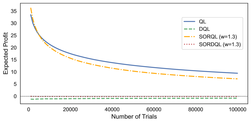
Figure 1: SOR with $w=1.3$.

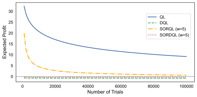
Figure 2: SOR with $w=5$.

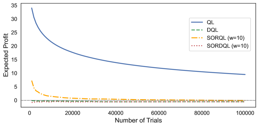
Figure 3: SOR with $w=10$.

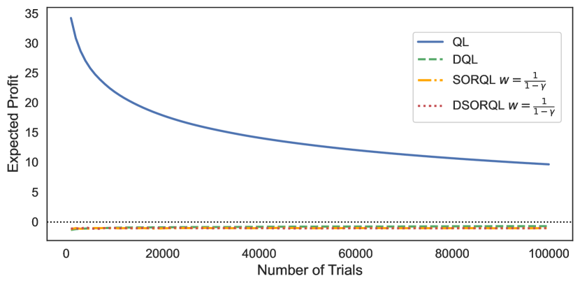
Figure 4: SOR with $w=w^{*}=1/(1-\gamma)$.

V-A Tabular version

This subsection provides numerical comparisons between Q-learning (QL), double Q-learning (DQL), model-free SOR Q-learning (MF-SORQL), and model-free double SOR Q-learning (MF-DSORQL). More specifically, we compare the above-mentioned algorithms on benchmark examples used in [8], namely roulette and grid world. Note that the step size for all the algorithms is the same, and all the other parameters used in the experiments are similar to [8].

V-A1 Roulette

In roulette, a player can choose from $170$ different betting actions, such as betting on a specific number or on the color black or red. Each bet has a payout designed so that the expected return is approximately $0.947 per dollar wagered, resulting in an expected loss of $-0.053 per play. This is modeled as an MDP with one state and $171$ actions, where one action is not placing a bet, ending the episode. If the player chooses not to bet, the payout is $0. Assuming the player bets $1 each time, the optimal strategy is to refrain from gambling, resulting in an expected profit of $0. In this example, the choice of successive relaxation factor $w$ is known as we have only one state. More specifically, $0<w\leq w^{*}=\frac{1}{1-\gamma\min_{i,a}p^{i}_{ia}}=\frac{1}{1-\gamma}$. Therefore, both MF-DSORQL and MF-SORQL are the same as that of DSORQL and SORQL, respectively. The experiment is conducted with $\gamma=0.95$, and the polynomial step-size mentioned in [8]. Fig. 4,4,4, and 4, presents the behavior of the proposed algorithms for various choices of SOR parameters and compares them with QL and DQL. Each experiment consists of $100000$ trails, and the graph is plotted by taking the average over $10$ independent experiments. It is evident from the plot that the performance of DSORQL is consistent for various choices of $w$, whereas the performance of the SORQL algorithm improves as $w$ gets closer to $w^{*}$. Further, the over-estimation bias of the SORQL algorithm is visible when $w=1.3$ (Fig. 4) and $w=5$ (Fig. 4). It is also interesting to see that, in Fig. 4., the over-estimation bias is not visible as this is a special case wherein $w=w^{*}=\frac{1}{1-\gamma}$, and since the next state $j$ will be $i$, Equation (6) reduces to the following:

$$Q_{n+1}(i,a) =(1-\beta_{n}(i,a))Q_{n}(s,a)+\beta_{n}(i,a)\left(\frac{r^{i}_{ia}}{1-\gamma}\right).$$

Therefore, in this particular case, the maximum operator gets canceled, and this is the reason for the behavior in Fig. 4. Note that in this classic example, the performance of the proposed DSORQL and DQL are almost the same.

V-A2 Grid World

Consider a $3\times 3$ grid world MDP. The agent can choose from four actions along four directions. The agent starts in the fixed starting state from one corner, with the goal state in the diagonally opposite corner. If the agent’s actions lead off the grid, it will stay in the same state. For every non-terminal step, the agent receives a random reward of either $-12$ or $+10$ with a probability of $0.5$ each. If the agent reaches the goal state, then any action from the goal state will end the episode with a reward of $+5$. The optimal policy concludes the episode after five actions, achieving an average reward of $+0.2$ per step. In order for this MDP to satisfy the requirement of $p^{i}_{ia}>0,\forall(i,a)\in S\times A$. The MDP is modified so that for any action chosen by the agent, there is a $0.9$ probability of transitioning to the next state according to the chosen action, and the agent stays in the same state with $0.1$ probability. Fig. 5 shows the average reward per step over $10000$ independent experiments. From Fig. 5, it is evident that the proposed MF-DSORQL outperforms MF-SORQL, QL, and DQL by obtaining a higher reward per step. Also, in this example, both QL and MF-SORQL show similar results, but neither is performing effectively.

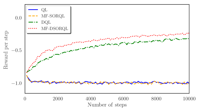
Figure 5: The performance of algorithms on grid world example.

V-B Deep RL version

This subsection compares the proposed double SOR Q-network (DSORDQN) with the deep RL version of SOR Q-learning (SORDQN) [17], the deep Q-network (DQN) [16], and the deep double Q-network (DDQN) [24]. The performance is evaluated using the maximization bias example [23], the LunarLander domain [22], and the classic CartPole environment [22]. The choice of SOR parameter $w$ for both SORDQN and DSORDQN is $1.3$ in all the experiments.

V-B1 Maximization Bias Example

This example is similar to the classic scenario used to illustrate bias behavior in tabular QL and DQL, which is discussed in Chapter 6 of [2]. However, the current implementation is adapted from [23]. Specifically, the maximization bias example in this manuscript involves $\{0,1,2,...,M\}$ states with $M=10^{9}$ and one terminal state. Therefore, applying tabular methods is infeasible. Consequently, we apply the proposed DSORDQN algorithm and compare its performance with DQN, SORDQN, and DDQN. The agent always begins in state zero. The discount factor is $\gamma=0.999$. Each state allows two actions: moving left or right. If the agent moves right from state zero, it receives zero reward, and the game ends. If the agent moves left, it transitions to one of the states in $\{1,2,...,M\}$ with equal probability and receives zero reward. In these new states, moving right returns the agent to state zero, while moving left ends the game, with rewards drawn from a Gaussian distribution $N(-0.1,1)$. Note that the choice of parameters in this example is the same as that of [23]. In other words, a fully connected neural network with two hidden layers of dimension $4$ and $8$ is used to approximate the Q-function. The activation function is ReLU, and the optimizer is stochastic gradient descent with no momentum. The policy used is epsilon-greedy with $\epsilon=0.1$, with training conducted over $400$ episodes. We plot the probability of selecting the left action from state zero at the end of each episode, averaging over $1000$ runs. A higher probability of choosing left suggests that the algorithm is following a sub-optimal strategy, as consistently choosing right yields the highest mean reward. In Fig. 6, one can observe that the policy obtained from the proposed algorithm is better than DQN, SORDQN, and DDQN.

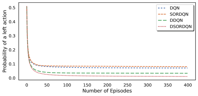
Figure 6: The performance of algorithms on maximization bias example.

V-B2 CartPole and LunarLander Environment

In the CartPole-v0 environment, the goal is to balance a pole on a moving cart by applying forces in the left and right direction on the cart. The agent receives a reward of $+1$ for each time step the pole remains upright, and the episode terminates if the pole angle is not in the range of $\pm 12^{\circ}$ or the cart range is not within $(-2.4,2.4)$. The standard threshold for a successful CartPole-v0 agent is to achieve an average reward of $195$ over $100$ episodes. In contrast, the LunarLander-v2 environment involves controlling a spacecraft to land safely on a lunar surface. The agent is rewarded for maintaining the lander within the landing pad, controlling its orientation, and landing with minimal velocity. The threshold for LunarLander-v2 is to achieve an average reward of $200$ over $100$ episodes. Both environments serve as tests for algorithms to demonstrate the ability to make decisions at varying complexity levels. The parameter selection and the implementation are taken from [26]. Specifically, the input layer has nodes of dimension state size, followed by two hidden layers with $64$ nodes each, using ReLU activation. The output layer has nodes of dimension action space. The optimizer used is Adam, and the policy is epsilon-greedy with decaying epsilon. The batch size is $64$, $\gamma$ is $0.99$, and the buffer size is $100,000$. Table I provides the performance of the proposed DSORDQN in comparison to the existing algorithms. It is evident from the table that the proposed algorithm completes both tasks with the minimum number of episodes compared to all the other algorithms.

Algorithm	CartPole	LunarLander
DQN	1000	1101
DDQN	3526	853
SORDQN	2343	826
DSORDQN	947	546

TABLE I: Number of episodes required to complete.

VI Conclusion

Motivated by the recent success of SOR methods in Q-learning and the issues concerning its over-estimation bias, this manuscript proposes a double successive over-relaxation Q-learning. Both theoretically and empirically, the proposed algorithm demonstrates a lower bias compared to SOR Q-learning. In the tabular setting, convergence is proven under suitable assumptions using SA techniques. A deep RL version of the method is also presented. Experiments on standard examples, including roulette, grid-world, and popular gym environments, showcase the algorithm’s performance. It is worth mentioning that, similar to the boundedness of iterates observed in Q-learning [27], investigating the boundedness of the proposed algorithms in the tabular setting presents an interesting theoretical question for future research.

References

- [1] M. L. Puterman, Markov decision processes: discrete stochastic dynamic programming. John Wiley & Sons, Inc., New York, 1994.
- [2] R. S. Sutton and A. G. Barto, Reinforcement Learning: An Introduction, 2nd ed. MIT Press, Cambridge, MA, 2018.
- [3] C. J. Watkins and P. Dayan, “Q-learning,” Mach. Learn., vol. 8, no. 3, pp. 279–292, 1992.
- [4] H. Xie and J. C. Lui, “A reinforcement learning approach to price cloud resources with provable convergence guarantees,” IEEE Trans. Neural Netw. Learn. Syst., vol. 33, no. 12, pp. 7448–7460, 2021.
- [5] C. Liu and Y. L. Murphey, “Optimal power management based on Q-learning and neuro-dynamic programming for plug-in hybrid electric vehicles,” IEEE Trans. Neural Netw. Learn. Syst., vol. 31, no. 6, pp. 1942–1954, 2019.
- [6] J. Wu, Y. Sun et al., “A Q-learning approach to generating behavior of emotional persuasion with adaptive time belief in decision-making of agent-based negotiation,” Inform. Sci., vol. 642, p. 119158, 2023.
- [7] Y. Zhang, Y. Cheng et al., “Long-/short-term preference based dynamic pricing and manufacturing service collaboration optimization,” IEEE Trans. Ind. Inform., vol. 18, no. 12, pp. 8948–8956, 2022.
- [8] H. Hasselt, “Double Q-learning,” Advances Neural Inf. Process. Syst., vol. 23, 2010.
- [9] D. Lee and W. B. Powell, “Bias-corrected Q-learning with multistate extension,” IEEE Trans. Automat. Control, vol. 64, no. 10, pp. 4011–4023, 2019.
- [10] C. Kamanchi, R. B. Diddigi, and S. Bhatnagar, “Successive over-relaxation Q-learning,” IEEE Control Syst. Lett., vol. 4, no. 1, pp. 55–60, 2019.
- [11] M. G. Azar, R. Munos, M. Ghavamzadaeh, and H. J. Kappen, “Speedy Q-learning,” Advances Neural Inf. Process. Syst., 2011.
- [12] D. Wu, X. Dong, J. Shen, and S. C. Hoi, “Reducing estimation bias via triplet-average deep deterministic policy gradient,” IEEE Trans. Neural Netw. Learn. Syst., vol. 31, no. 11, pp. 4933–4945, 2020.
- [13] D. Reetz, “Solution of a Markovian decision problem by successive overrelaxation,” Z. Operations Res. Ser. A-B, vol. 17, no. 1, pp. A29–A32, 1973.
- [14] I. John, C. Kamanchi, and S. Bhatnagar, “Generalized speedy Q-learning,” IEEE Control Syst. Lett., vol. 4, no. 3, pp. 524–529, 2020.
- [15] R. B. Diddigi, C. Kamanchi, and S. Bhatnagar, “A generalized minimax Q-learning algorithm for two-player zero-sum stochastic games,” IEEE Trans. Automat. Control, vol. 67, no. 9, pp. 4816–4823, 2022.
- [16] V. Mnih, K. Kavukcuoglu, D. Silver et al., “Playing atari with deep reinforcement learning,” arXiv preprint arXiv:1312.5602, 2013.
- [17] I. John and S. Bhatnagar, “Deep reinforcement learning with successive over-relaxation and its application in autoscaling cloud resources,” in International Joint Conference on Neural Networks, 2020, pp. 1–6.
- [18] J. N. Tsitsiklis, “Asynchronous stochastic approximation and Q-learning,” Mach. Learn., vol. 16, pp. 185–202, 1994.
- [19] T. Jaakkola, M. I. Jordan, and S. P. Singh, “On the convergence of stochastic iterative dynamic programming algorithms,” Neural Comput., vol. 6, no. 6, pp. 1185–1201, 1994.
- [20] V. S. Borkar, Stochastic approximation:A dynamical systems viewpoint. Cambridge University Press, 2008.
- [21] S. Singh, T. Jaakkola, M. L. Littman, and C. Szepesvári, “Convergence results for single-step on-policy reinforcement-learning algorithms,” Mach. Learn., vol. 38, no. 3, pp. 287–308, 2000.
- [22] G. Brockman, V. Cheung et al., “OpenAI Gym,” arXiv preprint arXiv:1606.01540, 2016.
- [23] W. Weng, H. Gupta et al., “The mean-squared error of double Q-learning,” Advances Neural Inf. Process. Syst., vol. 33, pp. 6815–6826, 2020.
- [24] H. Van Hasselt, A. Guez, and D. Silver, “Deep reinforcement learning with double Q-learning,” in Proceedings of the AAAI conference on artificial intelligence, vol. 30, no. 1, 2016.
- [25] S. R. Shreyas, “Double SOR Q-learning,” https://github.com/shreyassr123/Double-SOR-Q-Learning.
- [26] D. R. Pugh, “Improving the DQN algorithm using double Q-learning,” https://github.com/davidrpugh/stochastic-expatriate-descent.
- [27] A. Gosavi, “Boundedness of iterates in Q-learning,” Systems Control Lett., vol. 55, no. 4, pp. 347–349, 2006.