PharmacoMatch: Efficient 3D Pharmacophore Screening through Neural Subgraph Matching

Abstract

The increasing size of screening libraries poses a significant challenge for the development of virtual screening methods for drug discovery, necessitating a re-evaluation of traditional approaches in the era of big data. Although 3D pharmacophore screening remains a prevalent technique, its application to very large datasets is limited by the computational cost associated with matching query pharmacophores to database ligands. In this study, we introduce PharmacoMatch, a novel contrastive learning approach based on neural subgraph matching. Our method reinterprets pharmacophore screening as an approximate subgraph matching problem and enables efficient querying of conformational databases by encoding query-target relationships in the embedding space. We conduct comprehensive evaluations of the learned representations and benchmark our method on virtual screening datasets in a zero-shot setting. Our findings demonstrate significantly shorter runtimes for pharmacophore matching, offering a promising speed-up for screening very large datasets.

Keywords Contrastive representation learning  $\cdot$ Order embedding space  $\cdot$ Virtual screening  $\cdot$ Pharmacophore modeling

1 Introduction

A challenging task in the early stages of drug discovery campaigns is the identification of hit molecules that effectively bind to a protein target of interest. Due to the vastness of the chemical space, estimated to encompass more than $10^{60}$ small organic molecules (Virshup et al. 2013), identifying molecules with desirable drug-like properties is often compared to finding a needle in a haystack. Virtual screening methods have therefore become an essential component of the computer-aided drug discovery toolkit, aiding medicinal chemists in filtering molecular databases to efficiently explore the search space for potential hit compounds (Sliwoski et al. 2014).

A pharmacophore represents non-bonding interactions of chemical features that are essential for binding to a specific protein target (Wermuth et al. 1998). A pharmacophore query can, for example, be generated from the interaction profile of a ligand-receptor complex and used to identify potential hit compounds from databases by searching for molecules with similar pharmacophoric patterns (Wolber and Langer 2005). The process involves a positional alignment of the pharmacophore model with the three-dimensional conformations of molecules in the database, which are ranked based on their agreement with the pharmacophore query (Wolber, Dornhofer, and Langer 2006). Since pharmacophore screening focuses on abstract interaction patterns, rather than specific molecular structures, it allows for the identification of structurally diverse hit compounds (Seidel et al. 2017).

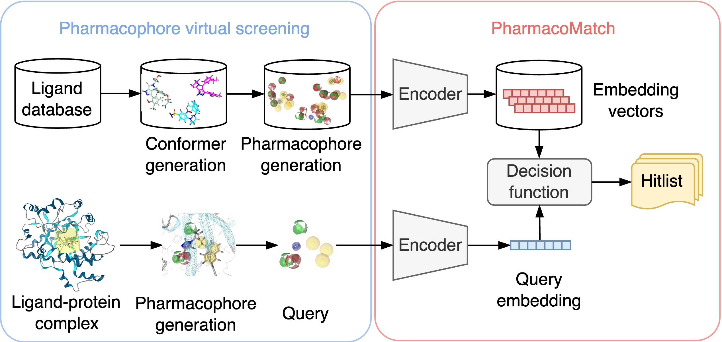
Figure 1: Overview of the PharmacoMatch workflow: Conformer and pharmacophore generation from ligands and query creation, for example from a ligand-protein complex, precede pharmacophore screening. The encoder model converts the screening database into embedding vectors, stored for later use. A hitlist is generated by comparing the query embedding with the database embeddings.

Virtual screening of make-on-demand libraries like Enamine REAL (Shivanyuk et al. 2007) is of growing interest because these libraries contain compounds that can be synthesized through reliable synthetic routes within a short period, making them readily commercially available. These libraries encompass billions of molecules and continue to expand due to advances in synthetic accessibility (Llanos et al. 2019). While screening larger compound libraries enhances the likelihood of identifying hit compounds, it also extends screening times, thereby necessitating the scaling up of virtual screening methods (Sadybekov et al. 2022). However, scaling up 3D pharmacophore screening to accommodate billions of molecules presents significant challenges (Warr et al. 2022). Although various filtering techniques have been developed (Seidel et al. 2010), molecules that pass these methods must still undergo alignment algorithms, which ultimately determine the speed of the process. Despite substantial efforts to optimize these algorithms (Wolber et al. 2008; Permann, Seidel, and Langer 2021), the overall screening procedure remains time-intensive.

In this work, we propose using self-supervised learning to create meaningful 3D pharmacophore representations for efficient virtual screening. Our PharmacoMatch model employs a graph neural network (GNN) encoder, trained with a contrastive learning objective, to map 3D pharmacophores into an order embedding space (Ying et al. 2020), thereby enabling pharmacophore matching through vector comparisons. The embedding vectors for the screening database are computed once and then used to quickly generate a hitlist based on the query embedding. An overview of the workflow is presented in Figure 1.

Our key contributions are:

• We develop a GNN encoder model that generates meaningful vector representations from 3D pharmacophores. The model is trained in a self-supervised manner on unlabeled data, employing a contrastive loss objective to capture the relationships between queries and targets based on their partial ordering in the learned embedding space.

• We use the learned representation for fast virtual screening in the embedding space and evaluate the performance of our method through experiments on virtual screening benchmark datasets.

2 Related work

Pharmacophore alignment algorithms

Alignment algorithms compute a rigid-body transformation, the pharmacophore alignment, to match a query’s pharmacophoric pattern to database ligands. A scoring function then evaluates the pharmacophore matching by considering both the number of matched features and their spatial proximity. The alignment is typically preceded by fast filtering methods that prune the search space based on pharmacophoric types, pharmacophoric point counts, and quick distance checks. Only molecules that pass these filters undergo the final, computationally expensive 3D alignment step, which is usually performed by minimizing the root mean square deviation (RMSD) between pairs of pharmacophoric points (Seidel et al. 2010; Dixon et al. 2006). The algorithm by Wolber, Dornhofer, and Langer (2006) creates smoothed histograms from the neighborhoods of pharmacophoric points for pair assignment using the Hungarian algorithm, followed by alignment with Kabsch’s method (Kabsch 1976). A recent implementation by Permann, Seidel, and Langer (2021) improves on runtime and accuracy by using a search strategy that maximizes pairs of matching pharmacophoric points. Alternatively, shape-matching algorithms like ROCS (Hawkins, Skillman, and Nicholls 2007) and Pharao (Taminau, Thijs, and De Winter 2008) model pharmacophoric points with Gaussian volumes, optimizing for volume overlap.

Machine learning for virtual screening

A common approach to using machine learning for virtual screening is to train models on measured bioactivity values. However, these models are constrained by the scarcity of experimental data, which is both costly and challenging to obtain (Li et al. 2021). Unsupervised training of target-agnostic models for virtual screening avoids dependence on labeled data, but remains relatively unexplored. DrugClip (Gao et al. 2023) approaches virtual screening as a similarity matching problem between protein pockets and molecules, using a multi-modal learning approach where a protein and a molecule encoder create a shared embedding space for virtual screening. Sellner, Mahmoud, and Lill (2023) used the Schrödinger pharmacophore shape-screening score to train a transformer model on pharmacophore similarity, which is a different objective than pharmacophore matching. PharmacoNet (Seo and Kim 2023) uses instance segmentation for pharmacophore generation in protein binding sites and a graph-matching algorithm for binding pose estimation, employing deep learning for pharmacophore modeling, but not for the alignment nor matching.

Contrastive representation learning

A common approach for the extraction of vector embeddings is the use of contrastive learning frameworks. These frameworks make use of a Siamese network architecture and a contrastive loss function, where an embedding space is learned by comparing positive and negative examples (Bengio, Courville, and Vincent 2013). In the last years, the computer vision community reported great improvements in the use of self-supervised learning (SSL) frameworks, which can be seen as a special case of contrastive learning. Instead of labels, these frameworks use augmentations to create positive and negative examples during training, which allows to train models on large datasets of unlabeled data. SSL is often used for model pretraining, followed by fine-tuning through supervised learning, which is especially useful when data is limited; however, the learned representations can also be utilized without fine-tuning if no labeled data is available (Balestriero et al. 2023).

3 Preliminaries

Pharmacophore representation

In this work, we treat 3D pharmacophores as attributed point clouds (Mahé et al. 2006; Kriege and Mutzel 2012). A pharmacophore $P$ can be represented by a set of pharmacophoric points $P=\{(\mathbf{r}_{i},l_{i})\in\mathbb{R}^{3}\times\mathcal{L}\}_{i}$ with the Cartesian coordinates $\mathbf{r}_{i}$ and the label $l_{i}$ of the pharmacophoric point $p_{i}$. The label set $\mathcal{L}$ contains the following pharmacophoric descriptors: hydrogen bond donors (HBD) and acceptors (HBA), halogen bond donors (XBD), positive (PI) and negative electrostatic interaction sites (NI), hydrophobic interaction sites (H), and aromatic moieties (AR). Directed descriptors like HBD and HBA can be associated with a vector component, but for simplicity, we will omit this information in our study.

The pharmacophore $P$ can be represented as a complete graph $G(P)=(V_{P},E_{P},\lambda_{P})$, where $V_{P}=\{v_{1},...,v_{|P|}\}$ denotes the set of nodes with node attributes $\lambda_{P}(v_{i})=l_{i}$, and $E_{P}=V_{P}\times V_{P}$ denotes the set of edges, where $\lambda_{P}$ represents a labelling function $\lambda:V\cup E\rightarrow\mathcal{L}$ that assigns a label to the corresponding vertex $v$ or edge $e$. The edges are undirected, edge $e_{uv}$ can be identified with edge $e_{vu}$, and the label of $e_{uv}$ is the pair-wise Euclidean distance $\lambda_{P}(e_{uv})=\lVert\mathbf{r}_{u}-\mathbf{r}_{v}\rVert_{2}$ between the positions of nodes $u$ and $v$. This representation is invariant to translation and rotation.

Subgraph matching

Two graphs $G_{1}=(V_{1},E_{1},\lambda_{1})$ and $G_{2}=(V_{2},E_{2},\lambda_{2})$ are isomorphic, denoted by $G_{1}\simeq G_{2}$, if there exists an edge-preserving bijection $f:V_{1}\rightarrow V_{2}$ such that $\forall(u,v)\in E_{1}:(f(u),f(v))\in E_{2}$. Additionally, we require the preservation of node and edge labels, such that $\forall v\in V_{1}:\lambda_{1}(v)=\lambda_{2}(f(v))$, and $\forall(u,v)\in E_{1}:\lambda_{1}((u,v))=\lambda_{2}((f(u),f(v)))$. Let $G_{Q}=(V_{Q},E_{Q},\lambda_{Q})$ be a query graph, $G_{T}=(V_{T},E_{T},\lambda_{T})$ a larger target graph, and $G_{H}=(V_{H},E_{H},\lambda_{H})$ a subgraph of $G_{T}$ such that $V_{H}\subseteq V_{T}$, and $E_{H}\subseteq E_{T}$. The objective of subgraph matching is to decide, whether $G_{Q}$ is subgraph isomorphic to $G_{T}$, denoted by $G_{Q}\lesssim G_{T}$, which requires the existence of a non-empty set of subgraphs $\mathcal{H}=\{G_{H}\mid G_{H}\simeq G_{Q}\}$ that are isomorphic to $G_{Q}$.

Pharmacophore matching

In its most general setting, pharmacophore matching seeks to match all pharmacophoric points of a query pharmacophore $P_{Q}$ with the corresponding pharmacophoric points of a larger target pharmacophore $P_{T}$.

Let $P_{H}\subseteq P_{T}$ denote a subset of the pharmacophoric points of $P_{T}$. Then $P_{Q}$ matches $P_{T}$ after alignment if there exists a bijection $g:P_{Q}\rightarrow P_{H}$ such that $\forall i\in P_{Q}:l_{i}=l_{g(i)}$ and $\lVert\mathbf{r}_{i}-\mathbf{r}_{g(i)}\rVert_{2}<r_{T}$, where $r_{T}$ is the radius of a tolerance sphere. It is thereby sufficient that query pharmacophoric points are mapped into the tolerance sphere of their target counterpart. For simplicity, we assume the same tolerance radii among all pharmacophoric points. The ultimate goal of pharmacophore matching is to retrieve molecules from a database. A matching pharmacophore is always linked to a corresponding ligand molecule via a look-up table.

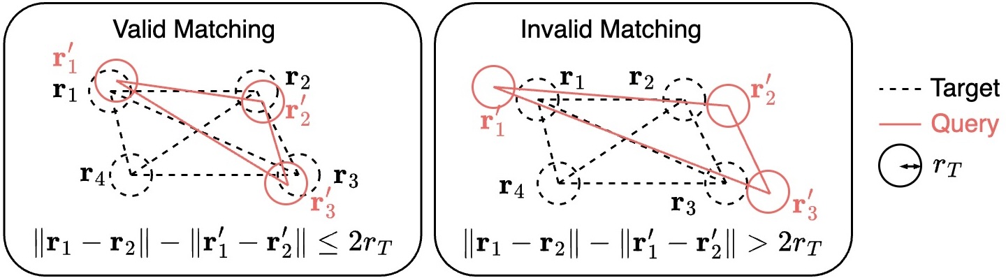
Figure 2: Illustration of the pharmacophore matching objective: The aim is to match the pharmacophoric points of a query with the corresponding points of a target pharmacophore such that the query points fall within the tolerance sphere of the target points, with a tolerance radius $r_{T}$.

When represented as graphs $G_{Q}=G(P_{Q})$, $G_{H}=G(P_{H})$, and $G_{T}=G(P_{T})$, this task boils down to the node-induced subgraph matching of a query pharmacophore graph $G_{Q}$ to a target pharmacophore graph $G_{T}$. The tolerance sphere, however, weakens the requirement on edge label matching. An approximate matching $\lambda_{Q}((u,v))\approx\lambda_{H}((f(u),f(v)))$ is sufficient if the difference between $\lambda_{Q}((u,v))$ and $\lambda_{H}((f(v),f(u)))$ is less than $2r_{T}$, where $r_{T}$ represents the tolerance radius of each pharmacophoric point. This ensures that the query points fall within the tolerance spheres of the target points (compare Figure 2). Our problem formulation of pharmacophore matching relies on relative distances instead of the absolute positioning of pharmacophoric features and is therefore independent of prior alignment.

4 Methodology

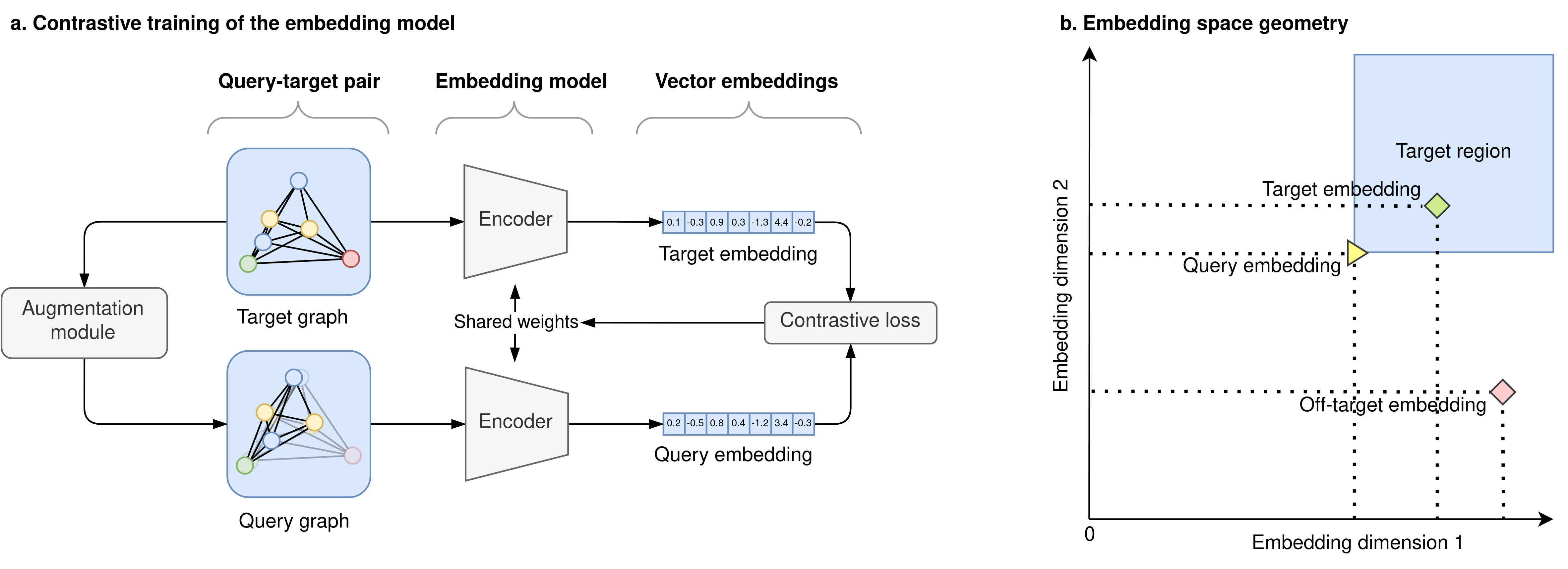
Figure 3: (a.) The embedding model learns an order embedding space by comparing augmented pharmacophores. (b) Illustration of the embedding space, where pharmacophores matching a query are positioned to the upper right.

Overview

In the following we introduce PharmacoMatch, a novel contrastive learning framework with the aim to encode query-target relationships of 3D pharmacophores into an embedding space. We propose to train a GNN encoder model in a self-supervised fashion, as illustrated in Figure 3. Our model is trained on approximately 1.2 million unlabeled small molecules from the ChEMBL database (Davies et al. 2015; Zdrazil et al. 2023) and learns pharmacophore matching solely from augmented examples, comparing positive and negative pairs of query and target pharmacophore graphs, while optimizing an order embedding loss to extract relevant matching patterns.

Unlabeled data for contrastive training

To span the pharmaceutical compound space, we download a set of drug-like molecules sourced from the ChEMBL (2024) website in the form of Simplified Molecular Input Line Entry System (SMILES) strings (Weininger 1988) and curate an unlabeled dataset using the open-source Chemical Data Processing Toolkit (CDPKit) (Seidel 2024) (see Appendix A.1 for details). After an initial data clean-up, which includes the removal of solvents and counter ions, adjustment of protonation states to a physiological pH, and elimination of duplicate structures, the dataset contains approximately 1.2 million small molecules. To ensure a zero-shot setting in our validation experiments, we remove all molecules from the training data that also appear in the test sets. Finally, we generate a low-energy 3D conformation and the corresponding pharmacophore for each ligand.

Model input

We represent the node labels $\lambda_{P}(V_{P})$ of a given pharmacophore graph $G(P)=(V_{P},E_{P},\lambda_{P})$ as one-hot-encoded (OHE) feature vectors $\mathbf{h}=(\mathbf{h}_{1},...,\mathbf{h}_{|P|})$. We employ a distance encoding to represent pair-wise distances, which was inspired by the SchNet architecture (Schütt et al. 2018). The edge attributes of edge $e_{uv}$ are derived from the edge label $\lambda_{P}(e_{uv})$ and represented by a radial basis function $\mathbf{e}_{k}(\mathbf{r}_{u}-\mathbf{r}_{v})=\exp(-\beta(\lVert\mathbf{r}_{u}-\mathbf{r}_{v}\rVert_{2}-{\mu}_{k})^{2})$, where centers $\mu_{k}$ were taken from a uniform grid of $K$ points between zero and the distance cutoff at 10 Å, and the smoothing factor $\beta$ represents a hyperparameter. To this end, the pharmacophore $P$ is represented by a data point $\mathbf{x}=[\mathbf{h},\mathbf{e}]$ which is a tuple of the feature matrix $\mathbf{h}\in\mathbb{R}^{|P|\times L}$ and the distance-encodings $\mathbf{e}\in\mathbb{R}^{(|P|\times|P|)\times K}$.

GNN encoder architecture

The encoder input is the pharmacophore graph representation $\mathbf{x}=[\mathbf{h},\mathbf{e}]$, with the feature matrix $\mathbf{h}$ and the edge attributes $\mathbf{e}$. Node feature embeddings are generated by initially passing the OHE feature matrix through a single dense layer without an activation function. We then update the node representations through message passing using the edge-conditioned convolution operator (NNConv) by Gilmer et al. (2017); Simonovsky and Komodakis (2017), which was originally designed for representation learning on point clouds and 3D molecules, to aggregate distance information into the learned node representations (see Appendix A.3 for details). We find that DenseNet-style skip-connections (Huang et al. 2017) are beneficial for learning robust representations. Graph-level read-out is achieved by additive pooling of the updated feature matrix $\mathbf{h}\in\mathbb{R}^{|P|\times m}$ into a graph representation $\mathbf{q}\in\mathbb{R}^{m}$, which is then projected to the final output embedding $\mathbf{z}\in\mathbb{R}^{D}_{+}$ by a multi-layer perceptron. The employed loss function requires to map the final representation to the non-negative real number space. We accomplish this by using the absolute values of the learnable weights for the last linear transformation immediately after the final ReLU unit (see Appendix A.4 for details).

Loss function

In order to encode query-targets relationship of pharmacophores into the embedding space, we employ the loss function by Ying et al. (2020). The key insight is that subgraph relationships can be effectively encoded in the geometry of an order embedding space through a partial ordering of the corresponding vector embeddings. Let $\mathbf{z}_{Q}$ the embedding of graph $G_{Q}$, $\mathbf{z}_{T}$ the embedding of graph $G_{T}$, and $f_{\Theta}:\mathcal{G}\rightarrow\mathbb{R}^{D}_{+}$ a GNN encoder to map pharmacophore graphs $\mathcal{G}$ to embedding vectors $\mathbf{z}\in\mathbb{R}^{D}_{+}$. The partial ordering $\mathbf{z}_{Q}\preceq\mathbf{z}_{T}$ reflects, whether $G_{Q}$ is subgraph isomorphic to $G_{T}$:

$$\mathbf{z}_{Q}[i]\leq\mathbf{z}_{T}[i],\;\forall i\in\{1,...,D\}\;\mathrm{iff}\;G_{Q}\lesssim G_{T}$$ (1)

The following max-margin objective can be used to train the GNN encoder $f_{\Theta}$ on this relation:

$$\mathcal{L}(\mathbf{z}_{Q},\mathbf{z}_{T})=\sum_{(\mathbf{z}_{Q},\mathbf{z}_{T})\in Pos}E(\mathbf{z}_{Q},\mathbf{z}_{T})+\sum_{(\mathbf{z}_{Q},\mathbf{z}_{T})\in Neg}\max\{0,\alpha-E(\mathbf{z}_{Q},\mathbf{z}_{T})\}$$ (2)

The penalty function $E:\mathbb{R}^{D}_{+}\times\mathbb{R}^{D}_{+}\rightarrow\mathbb{R_{+}}$ reflects violation of the partial ordering on the embedding vector pair:

$$E(\mathbf{z}_{Q},\mathbf{z}_{T})=\lVert\max\{\mathbf{0},\mathbf{z}_{Q}-\mathbf{z}_{T}\}\rVert_{2}^{2}$$ (3)

$Pos$ is the set of positive pairs per batch, these are pairs of query $\mathbf{z}_{Q}$ and target graph embedding $\mathbf{z}_{T}$ with a subgraph-supergraph relationship, and $Neg$ is the set of negative examples, these are pairs of query and target embedding vectors that violate this relationship. The positive and negative pairs are generated on-the-fly via augmentation during training.

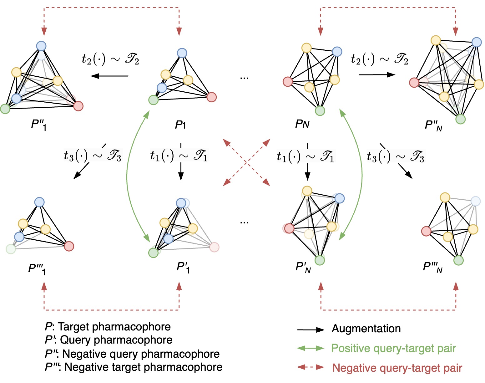
Figure 4: Augmentation strategies for model training involve generating positive and negative query-target pairs on-the-fly by combining node deletion with varying degrees of node displacement. Negative pairs are also created by shuffling the batch, mapping query pharmacophores to random target pharmacophores.

Augmentation module

The PharmacoMatch model correlates the matching of a query and a target pharmacophore with the partial ordering of their vector representations. Positive pairs represent successful matchings, while negative pairs serve as counter examples. In order to create these pairs from unlabeled training data, we define three families of augmentations $\mathcal{T}$, which are composed of random point deletions and positional point displacements.

For positive pairs, valid queries are created by randomly deleting some nodes from a pharmacophore $P$, leaving at least three, and displacing the remaining nodes within a tolerance sphere of radius $r_{T}$. This augmentation, denoted as $t_{1}(\cdot)\sim\mathcal{T}_{1}$, produces the positive pair $(t_{1}(P),P)$.

Negative pairs are used to show the model examples of unsuccessful matching, employing three strategies that illustrate different types of undesired outcomes. Our first strategy provides the model with examples of positional mismatch, by placing the pharmacophoric points of $P$ on the surface of the tolerance sphere without any point deletions. This augmentation, denoted by $t_{2}(\cdot)\sim\mathcal{T}_{2}$, is used to generate the negative query-target pair $(t_{2}(P),P)$.

Our second strategy teaches the model that every pharmacophoric point in the query should correspond to a point in the target. This is achieved by deleting some target nodes, using an augmentation operator $t_{3}(\cdot)\sim\mathcal{T}_{3}$, where $\mathcal{T}_{3}$ involves node deletion without displacement. As a result, the query in the pair $(t_{1}(P),t_{3}(P))$ only partially matches its target.

With the third strategy, we train the model to avoid matching queries with targets that are significantly different. This approach involves randomly mapping queries $t_{1}(P_{i})$ to the incorrect targets $P_{j}$, where $i\neq j$ (for more details, see Appendix A.2).

Curriculum learning

We design a curriculum learning strategy for training on pharmacophore graphs. We start training with pharmacophores containing four nodes. If the loss does not decrease significantly within 10 epochs, we add pharmacophores with one additional node to the training data. This approach allows the model to start with very simple examples, gradually increasing the difficulty of the matching task.

Model Training

Our GNN encoder model is implemented with three convolutional layers with an output dimension of 64. The MLP has a depth of three dense layers with a hidden dimension of 1024 and an output dimension of 512. The final model was trained for $500$ epochs using an Adam optimizer with a learning rate of $10^{-3}$. The margin of the best performing model was set to $\alpha=100$. The tolerance radius $r_{T}$ for node displacement was set to $1.5$ Å, which is the default value in the pharmacophore screening functionalities of the CDPKit (see Appendix A.5 for more details).

Decision function for model inference

We are using the trained GNN encoder $f_{\Theta}$ to precompute vector embeddings $\mathbf{z}_{T}$ of the database pharmacophores. These are queried with the pharmacophore embedding $\mathbf{z}_{Q}$ by verification of the partial ordering constraint (3), which shall not be violated by more than a threshold $t$. This leads to the decision function $g:\mathbb{R}^{D}_{+}\times\mathbb{R}^{D}_{+}\rightarrow\{0,1\}$:

$$g(\mathbf{z}_{Q},\mathbf{z}_{T})=\begin{cases}1&\mathrm{iff}E(\mathbf{z}_{Q},\mathbf{z}_{T})<t\\ 0&\mathrm{otherwise}\end{cases}$$ (4)

which evaluates to $1$ if the partial ordering on $\mathbf{z}_{Q}$ and $\mathbf{z}_{T}$ reflects a pharmacophore matching, and $0$ otherwise. In the following, we will refer to equation (4) as matching decision function. In practice, we recommend a decision threshold of $t=6500$, which was determined during our benchmark experiments.

5 Experiments

We designed our embeddings to reflect the type and relative positioning of pharmacophoric points. Comparison of embedding vectors via the matching prediction function should emulate the matching of the underlying pharmacophores. To get a better understanding of the encoder’s latent space, we investigate these properties as follows:

1. Pharmacophoric point perception: We investigate the learned embedding space quantitatively through dimensionality reduction.

2. Positional perception: We investigate the influence of positional changes on the output of the matching decision function.

3. Virtual screening performance: The performance of our model is evaluated using ten DUD-E targets, and the produced hitlists are compared with the performance and runtime of the CDPKit (Seidel 2024) alignment algorithm.

DUD-E benchmark dataset

We perform our experiments on the DUD-E benchmark dataset (Mysinger et al. 2012), which is commonly used to evaluate the performance of molecular docking and structure-based screening. The complete benchmark contains 102 protein targets, each accompanied by active and decoy ligands in the form of SMILES strings (Weininger 1988) and the PDB template (Burley et al. 2017) of the ligand-receptor complex. We randomly select ten different protein targets for the evaluation of our model. Ligands in these datasets are processed according to the data curation pipeline outlined in the Methodology section, except that we sample up to 25 conformations per compound. The ligand-receptor complex is used to generate a structure-based query with 5-7 pharmacophoric points (see Appendix A.6 for more details).

5.1 Pharmacophoric point perception

We conduct a quantitative analysis through dimensionality reduction to gain a first intuition for the properties of the learned embedding space.

The partial ordering of graph representations in the embedding space, based on the number of nodes per graph, is essential for encoding query-target relationships. This ordering property of the embedding space can be visualized using principal component analysis (PCA). Figure 5a displays the first two principal component axes of the learned representations, with the representations labeled according to the number of pharmacophoric points of the corresponding pharmacophore. This visualization demonstrates how the embedding vectors are systematically ordered relative to the number of nodes in each pharmacophore graph.

Similarly, the Uniform Manifold Approximation and Projection (UMAP) algorithm (McInnes, Healy, and Melville 2020), a dimensionality reduction technique that preserves the local neighborhood structure of high-dimensional data, was employed. Figure 5b shows the UMAP representation of the embeddings, labeled by the number of pharmacophoric points of a specific type. This visualization suggests that pharmacophores with a similar set of points are mapped proximally within the order embedding space.

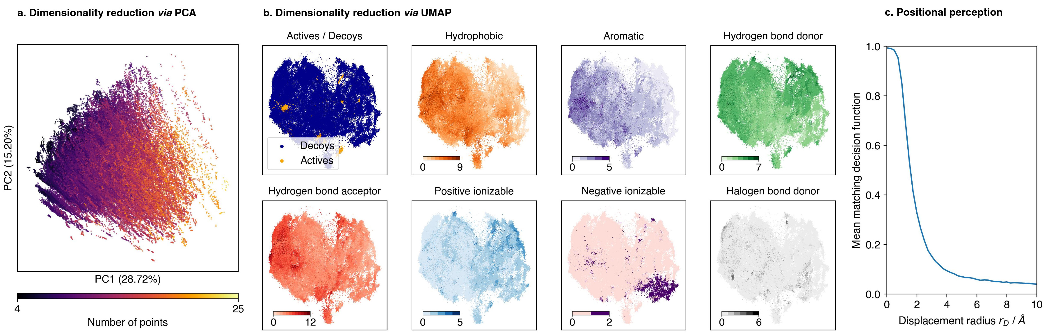
Figure 5: (a.) Dimensionality reduction of the ADA target’s embedding space via PCA, with embeddings labeled by pharmacophoric point count. (b.) Dimensionality reduction via UMAP, with embeddings labeled by pharmacophoric point type. (c.) Experimental validation of the model’s perception of 3D point positions, showing the mean matching decision function versus the displacement radius $r_{D}$ of the augmentation, with a decision threshold set to $t=6500$.

5.2 Positional perception

We define a family of augmentations $\mathcal{T}_{r_{D}}$ to randomly delete nodes from a pharmacophore $P$ and displace the remaining nodes by a radius $r_{D}$. We sample augmentations $t_{r_{D}}(\cdot)\sim\mathcal{T}_{r_{D}}$ with increasing radius $r_{D}$ taken from a uniform grid of $m$ distances between 0 and 10 Å.

For a given batch of pharmacophores $\{P_{1},...,P_{n}\}$, we generate the query-target pairs $\{(t_{r_{D}}(P_{1}),P_{1}),...,(t_{r_{D}}(P_{n}),P_{n})\}$. We then evaluate the decision function $g(\cdot,\cdot)$ (Equation 4) on the corresponding vector representations and calculate the mean of the decision function across all pairs against an increasing radius $r_{D}$, which is illustrated in Figure 5c.

Without node displacement, the mean matching decision function is close to 1, indicating that the model recognizes pharmacophores with reduced node sets as valid queries. With a displacement of approximately 1.5 Å, the mean matching decision value drops to 50%, demonstrating the model’s consideration of the chosen tolerance radius. Beyond a displacement of 1.5 Å, the decision function further decreases, approaching a plateau at approximately 6 Å. The results show that our model integrates 3D-positional information of pharmacophoric points into the learned representations.

5.3 Virtual screening

Each benchmark set is comprised of a pharmacophore query $P_{Q}$ and a set of ligands $\mathcal{L}=\{L_{1},...,L_{n}\}$, where each ligand $L_{i}$ is associated with a set of pharmacophores $\{P_{1},...,P_{k_{i}}\}_{i}$ and a label $y_{i}$, which indicates whether the ligand is active or decoy. The task is to rank the database ligands w.r.t. the query, based on a scoring function $F:\mathcal{P}\times\mathcal{P}\rightarrow\mathbb{R}_{+}$. The ranking score $\psi_{i}$ of ligand $L_{i}$ is calculated through aggregation of the pharmacophore scores $\bigoplus(\{F(P_{Q},P_{1}),...,F(P_{Q},P_{k_{i}})\}_{i})$, where $\bigoplus$ is an aggregation operator. PharmacoMatch transforms the query $G(P_{Q})\mapsto\mathbf{z}_{Q}$ and the set of pharmacophores $\{G(P_{1}),...,G(P_{k_{i}})\}_{i}\mapsto\{\mathbf{z}_{1},...,{\mathbf{z}}_{k_{i}}\}_{i}$ via encoder model $f_{\Theta}:\mathcal{G}\rightarrow\mathbb{R}^{D}_{+}$ and evaluates the penalty function $E:\mathbb{R}^{D}_{+}\times\mathbb{R}^{D}_{+}\rightarrow\mathbb{R_{+}}$. A low penalty corresponds to a high ranking. The ranking score of database ligand $L_{i}$ is calculated as $\psi_{i}=\min(\{E(\mathbf{z}_{Q},\mathbf{z}_{1}),...,E(\mathbf{z}_{Q},\mathbf{z}_{k_{i}})\}_{i})$.

Baseline algorithm

The baseline for our comparison is the alignment algorithm implemented in the open-source software CDPKit (Seidel 2024), which utilizes clique-detection followed by Kabsch alignment (Kabsch 1976). The alignment of a query $P_{Q}$ and a target $P_{T}$ is evaluated with an alignment score $S:\mathcal{P}\times\mathcal{P}\rightarrow\mathbb{R}_{+}$, which takes into account the number of matched features and their geometric fit (further details are provided in the Appendix A.6). The ligand ranking score is calculated as $\psi_{i}=\max(\{S(P_{Q},P_{1}),...,S(P_{Q},P_{k_{i}})\}_{i})$, the highest alignment score represents the score for the database ligand. Analogous to equation (4), we can also define a matching decision function $\phi$ based on the alignment score, where $t=|P_{Q}|$:

$$\phi(P_{Q},P_{T})=\begin{cases}1&\mathrm{iff}S(P_{Q},P_{T})\geq t\\ 0&\mathrm{otherwise}\end{cases}$$ (5)

Evaluation

Both algorithms rank database ligands to produce a hitlist. We assess the performance of PharmacoMatch on the benchmark using two approaches. First, we demonstrate that the PharmacoMatch penalty $E(\cdot,\cdot)$ correlates with the matching decision function $\phi(\cdot,\cdot)$ of the alignment algorithm. We evaluate both functions against all pharmacophores in a dataset w.r.t. query $P_{Q}$. The outputs are compared by generating the corresponding receiver operating characteristic (ROC) curves, and the performance is quantified using the area under the ROC curve (AUROC) metric.

Second, we compare the virtual screening performance of our model and the alignment algorithm using the ligand ranking score $\psi$. The primary objective of virtual screening is to find active compounds amongst decoys. We evaluate this using two different metrics. The AUROC metric is used to evaluate the overall classification performance w.r.t. activity label $y_{i}$. A drawback of this metric is that it does not reflect the early enrichment of active compounds in the hitlist, which is of significant interest in virtual screening. Early enrichment is assessed using the Boltzmann-enhanced discrimination of ROC (BEDROC) metric (Truchon and Bayly 2007), which assigns higher weights to better-ranked samples. Note that these performance metrics are entirely dependent on the chosen query. Rather than aiming to maximize those metrics, our goal is to achieve comparable values between our model and the alignment algorithm.

Screening performance

Our results, comparing PharmacoMatch with the alignment algorithm across all ten targets, are summarized in Table 1 (ROC plots are provided in the Appendix A.6). We observe a robust correlation between the hitlists generated by the two algorithms, demonstrating the effectiveness of our approach. This correlation varies by target, reflecting the sensitivity of virtual screening to the chosen query. Although the alignment algorithm achieves generally higher AUROC scores and early enrichment, our method consistently produces hitlists with competitive performance across several targets.

Table 1: Method comparison and screening performance of the PharmacoMatch algorithm and the CDPKit alignment algorithm on ten different DUD-E protein targets (see Appendix A.6 for details). BEDROC values are calculated with $\alpha=20$, as recommended by Truchon and Bayly (2007). Metrics are reported in percent. Confidence intervals are calculated using bootstrapping (Efron 1979), with standard deviations reported based on 1,000 resampled datasets.

Protein	Method	Screening Performance
Target	Comparison	PharmacoMatch		CDPKit
	AUROC	AUROC	BEDROC	AUROC	BEDROC
ACES	$90.7\pm 0.2$	$57\pm 2$	$19\pm 2$	$55\pm 1$	$15\pm 1$
ADA	$97.7\pm 0.3$	$80\pm 3$	$39\pm 4$	$93\pm 2$	$80\pm 4$
ANDR	$98.0\pm 0.2$	$78\pm 2$	$32\pm 2$	$72\pm 2$	$26\pm 2$
EGFR	$90.4\pm 0.5$	$59\pm 1$	$10\pm 1$	$72\pm 1$	$22\pm 1$
FA10	$84.2\pm 0.1$	$48\pm 1$	$2.1\pm 0.4$	$55\pm 1$	$5.8\pm 0.6$
KIT	$80.2\pm 0.1$	$52\pm 2$	$2.3\pm 0.6$	$58\pm 2$	$7\pm 1$
PLK1	$79.1\pm 0.5$	$61\pm 3$	$9\pm 2$	$75\pm 3$	$39\pm 3$
SRC	$95.6\pm 0.1$	$77\pm 1$	$22\pm 1$	$77\pm 1$	$24\pm 1$
THRB	$86.4\pm 0.4$	$73\pm 1$	$26\pm 2$	$81\pm 1$	$40\pm 2$
UROK	$83.3\pm 0.2$	$59\pm 2$	$3\pm 1$	$91\pm 1$	$52\pm 3$

Runtime comparison

In terms of runtime, PharmacoMatch significantly outperforms the alignment algorithm. We compare the time required for alignment, embedding, and vector matching per pharmacophore. Alignment is performed in parallel on an AMD EPYC 7713 64-Core Processor with 128 threads, while pharmacophore embedding and matching are run on an NVIDIA GeForce RTX 3090, with both devices having comparable purchase prices and release dates. Creating vector embeddings from pharmacophore graphs takes $92\pm 12~{}\mathrm{\mu s}$ per pharmacophore, which takes longer than aligning a query to a target with $13\pm 7~{}\mathrm{\mu s}$. However, the embedding process only needs to be performed once. Subsequently, the preprocessed vector data can be used for vector matching, which takes $0.30\pm 0.09~{}\mathrm{\mu s}$, being approximately two orders of magnitude faster than the alignment. Additionally, vector comparison is independent of the query size, an advantage not shared by the alignment algorithm. Although executed on different hardware, this comparison highlights the speed-gain of our algorithm.

Practical considerations

There are two options for integrating our model into a virtual screening pipeline. First, the PharmacoMatch model can be used in place of the alignment algorithm to generate a hitlist of ligands, which is suitable for quickly producing a compound list for experimental testing. Alternatively, our method can serve as an efficient prefiltering tool for very large databases, reducing the number of molecules from billions to millions, after which the slower alignment algorithm can be applied to this filtered subset. Note that alignment will still be necessary if visual inspection of aligned pharmacophores and corresponding ligands is desired.

6 Conclusion

We have presented PharmacoMatch, a contrastive learning framework that creates meaningful pharmacophore representations for virtual screening. The proposed method tackles the matching of 3D pharmacophores through vector comparison in an order embedding space, thereby offering a valuable method for significant speed-up of virtual screening campaigns. PharmacoMatch is the first machine-learning based solution that approaches pharmacophore virtual screening via an approximate neural subgraph matching algorithm. We are confident that our method will help to improve on existing virtual screening workflows and contribute to the assistance of medicinal chemist in the complex task of drug discovery.

Code & data availability

We will make our code publicly available upon acceptance via https://github.com/molinfo-vienna/PharmacoMatch and share the curated datasets via (https://zenodo.org/).

Author contributions

Conceptualization: DR, OW. Methodology: DR, OW. Data Curation & Analysis: DR. Code Implementation & Model Training: DR. CDPKit Software & Support: TS. Investigation: DR. Writing (Original Draft): DR. Writing (Review and Editing): DR, OW, TS, TL. Funding Acquisition: TL. Resources: TL. Supervision: OW, TL. All authors have given approval to the final version of the manuscript.

Competing interests

The authors declare no competing interests.

A Appendix

A.1 Dataset curation & statistics

Unlabeled training data was downloaded from the ChEMBL database to represent small molecules with drug-like properties. At the time of data download, the ChEMBL database contained 2,399,743 unique compounds. We constrained the compound category to "small molecules" and enforced adherence to the Lipinsky rule of five (Lipinski et al. 1997), specifically setting violations to "0," resulting in a refined set of 1,348,115 compounds available for download. The molecules were acquired in the form of Simplified Molecular Input Line Entry System (SMILES) (Weininger 1988) strings. Subsequent to data retrieval, we conducted preprocessing using the database cleaning functionalities of the Chemical Data Processing Toolkit (CDPKit) (Seidel 2024). This process involved the removal of solvents and counter ions, adjustment of protonation states to a physiological pH value, and elimination of duplicate structures, where compounds differing only in their stereo configuration were regarded as duplicates. To prevent data leakage, we carefully removed all structures from the training data that would occur in one of the test sets we used for our benchmark experiments. The final set was comprised of 1,221,098 compounds. For each compound within the dataset, a 3D conformation was generated using the CONFORGE (Seidel et al. 2023) conformer generator from the CDPKit, which was successful for 1,220,104 compounds. To enhance batch diversity, we generated only one conformation per compound for contrastive training. Subsequently, 3D pharmacophores were computed for each conformation, with removal of pharmacophores containing less than four pharmacophoric points. The ultimate dataset comprised 1,217,361 distinct pharmacophores.

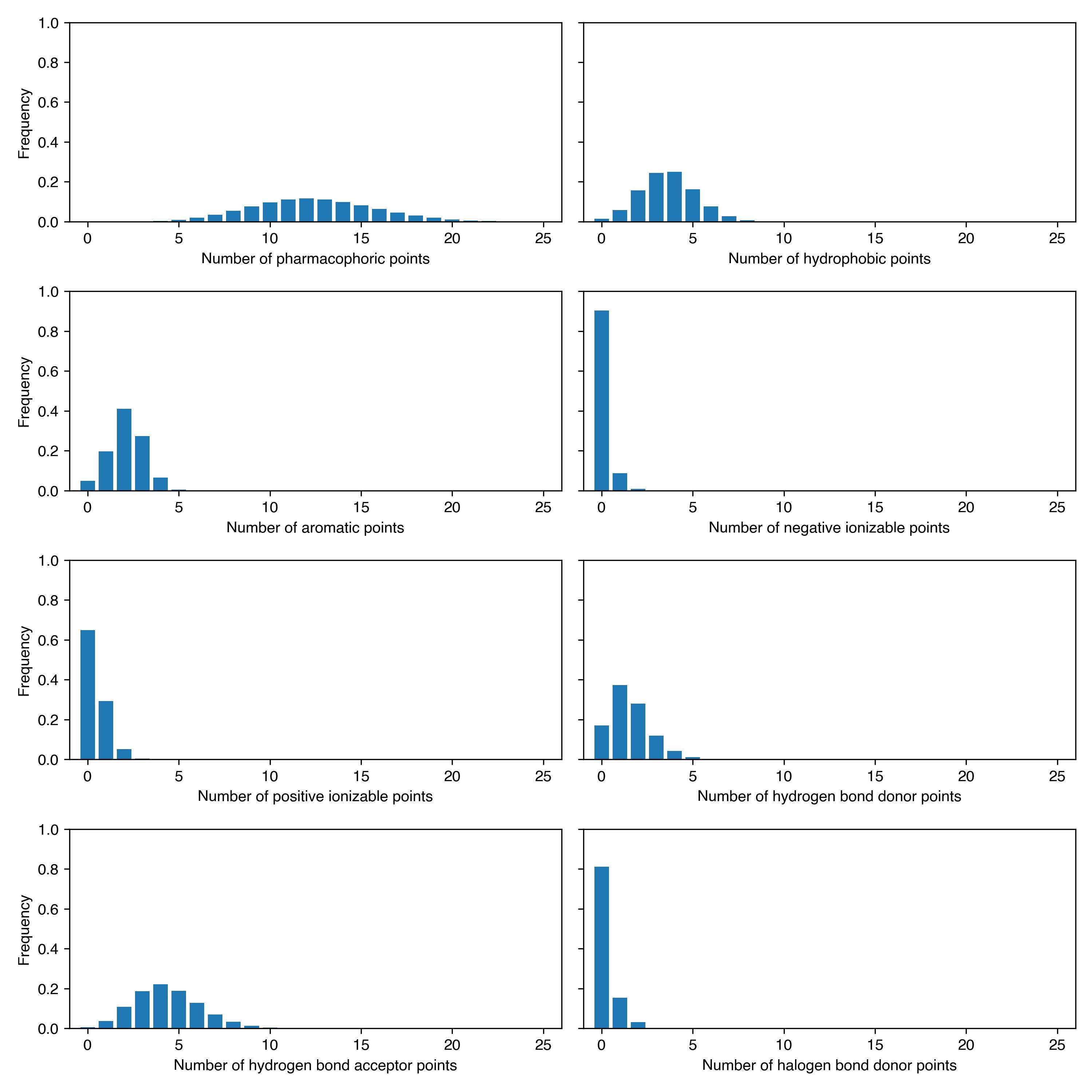
Figure A1: Pharmacophoric point statistics of the training data. The respective histograms display the total number of pharmacophoric points and the number of points of specific types per pharmacophore in the training data. The complete training dataset contains 1,217,361 distinct pharmacophores.

Figure A1 shows the frequency of pharmacophores with a specific pharmacophoric point count in the training data. On average, a pharmacophore consists of 13 pharmacophoric points, with the largest pharmacophore in the dataset containing 32 points. Pharmacophores with fewer than four points were omitted during data clean-up. Hydrophobic pharmacophoric points and hydrogen bond acceptors are the most prominent, while hydrogen bond donors and aromatics occur less frequently. Ionizable pharmacophoric points and halogen bond donors are comparatively rare.

A.2 Augmentation module

The augmentation module receives the initial pharmacophore $\mathbf{x_{0}}=[\mathbf{h_{0}},\mathbf{r_{0}}]$, with the initial OHE feature matrix $\mathbf{h_{0}}$ and the Cartesian coordinates $\mathbf{r_{0}}$. Edge attributes of the complete graph were calculated from the pair-wise distances between nodes after modifying the input according to the augmentation strategy, which combines random node deletion and random node displacement. The module outputs the modified tuple $\mathbf{x}=[\mathbf{h},\mathbf{e}]$ with the feature matrix $\mathbf{h}$ and the edge attributes $\mathbf{e}$.

Node deletion

Random node deletion involved removing at least one node, with the upper bound determined by the cardinality of the set of nodes $V_{i}$ of graph $G_{i}$. To ensure the output graph retained at least three nodes, the maximum number of deletable nodes was $|V_{i}|-3$. The number of nodes to delete was drawn uniformly at random.

Node displacement

There are two modes for the displacement of pharmacophoric points. Positive pairs were constructed by displacing the pharmacophoric points within the tolerance sphere of the initial pharmacophore. For simplicity, we assumed the same tolerance sphere radius $r_{T}$ across different pharmacophoric types. The coordinate displacement $(\Delta x,\Delta y,\Delta z)$ was created from spherical coordinates $\phi\sim\mathcal{U}(0,2\pi)$ and $\cos{\theta}\sim\mathcal{U}(-1,1)$, which were drawn at random from a uniform distribution. The coordinate displacement was calculated as

$$\Delta x=\Delta r\sin{\theta}\cos{\phi},~{}\Delta y=\Delta r\sin{\theta}\sin{\phi},~{}\Delta z=\Delta r\cos{\theta}$$ (6)

where $\Delta r=r_{T}\sqrt[3]{u}$ and $u\sim\mathcal{U}(0,1)$. Negative pairs were created by displacement of the nodes at the border of the tolerance sphere. This was achieved by random sampling from a sphere surface, i.e. with $u=1$.

A.3 Message passing neural network

Convolution on irregular domains like graphs is formulated as message passing, which can generally be described as:

$$\mathbf{h}_{i}^{(k)}=\gamma^{(k)}(\mathbf{h}_{i}^{(k-1)},\bigoplus_{j\in\mathcal{N}(i)}\phi^{(k)}(\mathbf{h}_{i}^{(k-1)},\mathbf{h}_{j}^{(k-1)},\mathbf{e}_{ij}))$$ (7)

where $\mathbf{h}_{i}^{(k)}\in\mathbb{R}^{F^{\prime}}$ denotes the node features of node $i$ at layer $k$, $\mathbf{h}_{i}^{(k-1)}\in\mathbb{R}^{F}$ denotes the node features of node $i$ at layer $k-1$, $\mathbf{e}_{ij}\in\mathbb{R}^{D}$ the edge features of the edge from node $i$ to node $j$, $\gamma^{(k)}$ and $\phi^{(k)}$ are parameterized, differentiable functions, and $\bigoplus$ is an aggregation operator like, e. g., the summation operator (Fey and Lenssen 2019). In our encoder architecture, we employed the following edge-conditioned convolution operator, which was proposed both by Gilmer et al. (2017); Simonovsky and Komodakis (2017):

$$\mathbf{h}_{i}^{(k)}=\Theta\mathbf{h}_{i}^{(k-1)}+\sum_{j\in\mathcal{N}(i)}\mathbf{h}_{j}^{(k-1)}\cdot\psi_{\Theta}(\mathbf{e}_{ij})$$ (8)

where $\Theta\in\mathbb{R}^{F\times F{{}^{\prime}}}$ denotes learnable weights and $\psi_{\Theta}(\cdot):\mathbb{R}^{D}\rightarrow\mathbb{R}^{F\times F{{}^{\prime}}}$ denotes a neural network, in our case an MLP with one hidden layer. These transformations map node features $\mathbf{h}$ into a latent representation that combines pharmacophoric types with distance encodings.

A.4 Encoder implementation

The encoder was implemented as a GNN $f_{\Theta}:\mathcal{G}\rightarrow\mathbb{R}_{+}^{D}$ that maps a given graph $G$ to the abstract representation vector $\mathbf{z}\in\mathbb{R}_{+}^{D}$. The architecture is comprised of an initial embedding block, three subsequent convolution blocks, followed by a pooling layer, and a projection block.

Embedding block

The embedding block receives the pharmacophore graph $G_{i}$ as the tuple $\mathbf{x}_{i}=[\mathbf{h}_{i},\mathbf{e}_{i}]$, with the OHE feature matrix $\mathbf{h}_{i}$ and the edge attributes $\mathbf{e}_{i}$. Initial node feature embeddings are created from the OHE features with a fully-connected (FC) dense layer with learnable weights $\mathbf{W}$ and bias $\mathbf{b}$:

$$\mathbf{h}_{i}\leftarrow\mathbf{W}\mathbf{h}_{i}+\mathbf{b}$$ (9)

Convolution block

The convolution block consists of a graph convolution layer, which is implemented as edge-conditioned convolution operator (NNConv), the update rule is described in Section A.3. The network further consists of batch normalization layers (BN), GELU activation functions, and dropout layers. The hidden representation $\mathbf{h}^{l}_{i}$ of graph $G_{i}$ is updated at block $l$ as follows:

$$[\mathbf{h}^{l}_{i},\mathbf{e}_{i}]\rightarrow\{\mathrm{NNConv}\rightarrow\mathrm{BN}\rightarrow\mathrm{GELU}\rightarrow\mathrm{concat}(\mathbf{h}^{l^{\prime}}_{i},\mathbf{h}^{l}_{i})\rightarrow\mathrm{dropout}\}\rightarrow\mathbf{h}^{l+1}_{i}$$ (10)

where $\mathbf{h}^{l^{\prime}}_{i}$ represents the latent representation after activation. Updating the feature matrix $l$ times yields the final node representations of the pharmacophoric points.

Pooling layer

We employed additive pooling for graph-level read-out $\mathbf{r}_{i}$, which aggregates the set of $|V|$ node representations $\{\mathbf{h}_{1},...,\mathbf{h}_{|V|}\}_{i}$ of a Graph $G_{i}$ by element-wise summation:

$$\mathbf{q}_{i}=\sum_{k=1}^{|V|}\mathbf{h}_{k}$$ (11)

Projection block

The projection block maps the graph-level read-out to the positive real number space and is implemented as a multi-layer perceptron $\mathrm{MLP}:\mathbb{R}^{d}\rightarrow\mathbb{R}_{+}^{D}$, where $d$ is the dimension of the vector representation before and $D$ the dimension after the projection. The block consists of $k$ sequential layers of FC layers, BN, ReLU activation, and dropout:

$$\mathbf{q}_{i}^{k}\rightarrow\{\mathrm{FC}\rightarrow\mathrm{BN}\rightarrow\mathrm{ReLU}\rightarrow\mathrm{Dropout}\}\rightarrow\mathbf{q}^{k+1}_{i}$$ (12)

The final layer is a FC layer without bias and with positive weights, only:

$$\mathbf{z}_{i}\leftarrow\mathrm{abs}(\mathbf{W})\mathbf{q}_{i}$$ (13)

Matrix multiplication of the positive learnable weights $\mathbf{W}$ and the output of the last ReLU activation function produces the final representation $\mathbf{z}_{i}\in\mathbb{R}_{+}^{D}$.

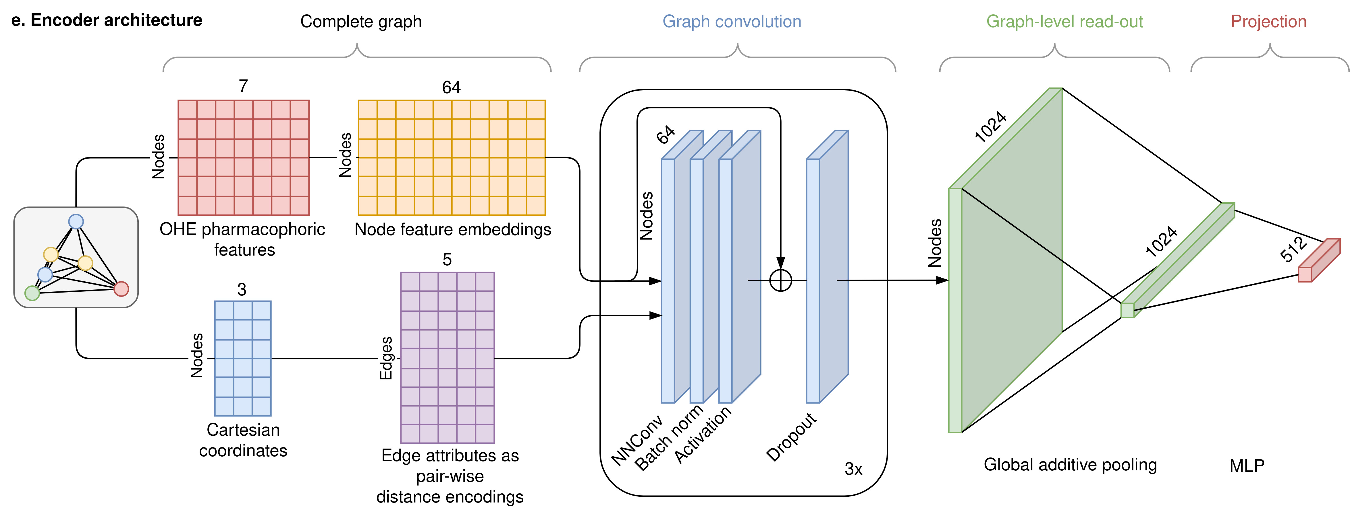
Figure A2: Architecture of the GNN encoder model.

A.5 Model implementation and training

Implementation dependencies

The GNN was implemented in Python 3.10 with PyTorch (v2.0.1) and the PyTorch Geometric library (v2.3.1) (Fey and Lenssen 2019). Both, model and dataset, were implemented within the PyTorch Lightning (Falcon and The PyTorch Lightning team 2019) framework (v2.1.0). Model training was monitored with Tensorboard (v2.13.0). CDPKit (v1.1.1) was employed for chemical data processing. Software was installed and executed on a Rocky Linux (v9.4) system with x86-64 architecture.

Model training

Training was performed on a single NVIDIA GeForce 3090 RTX graphics unit with 24 GB GDDR6X. Training runs were performed for a maximum of 500 epochs with a batch size of 256 pharmacophore graphs. Curriculum learning was applied by gradual enrichment of the dataset with increasingly larger pharmacophore graphs. At training start, only pharmacophore graphs with 4 nodes were considered. After 10 subsequent epochs without considerable minimization of the loss function, pharmacophore graphs with one additional node were added to the training data. The loss function was minimized with the Adam optimizer, we further applied gradient clipping. A training run on the full dataset took approximately 48 hours with the above hardware specifications.

Hyperparameter tuning & model selection

Hyperparameters were optimized through random parameter selection, the tested ranges are summarized in Table A2. Unlabeled data was split into training and validation data with a 98:2 ratio. Training runs were compared using the AUROC value on the validation data. This was calculated by treating the positive and negative pairs as binary labels, and the predictions were based on their respective order embedding penalty, which was calculated with Equation (3). Hyperparameter optimization was performed on a reduced dataset with 100,000 graphs, which took approximately 5 hours per run. The best performing models were retrained on the full dataset. The hyperparameters of the final encoder model are summarized in Table A1. After model selection, the final model performance was tested on virtual screening datasets.

Table A1: Hyperparameters of the best performing encoder model

Hyperparameter
batch size	256
dropout convolution block	0.2
dropout projection block	0.2
max. epochs	500
hidden dimension convolution block	64
hidden dimension projection block	1024
output dimension convolution block	1024
output dimension projection block	512
learning rate optimizer	0.001
margin for negative pairs	100.0
number of convolution blocks	3
depth of the projector MLP	3
edge attributes dimension	5
sampling sphere radius positive pairs	1.5
sampling surface radius negative pairs	1.5

Table A2: Tested hyperparameter ranges for model training.

Hyperparameter
dropout	[0.2, 0.3, 0.4, 0.5]
margin for negative pairs	[0.1, 0.5, 1, 2, 5, 10, 100, 1000]
output dimension projection block	[64, 128, 256, 512, 1024]
displacement sphere radius $r_{T}$ of positive pairs	[0.25, 0.5, 1.0, 1.5]

A.6 Virtual screening

DUD-E dataset details

General information about the DUD-E targets is summarized in Table A3. For each target we downloaded the receptor structure from the PDB and created the corresponding interaction pharmacophore with the CDPKit. Vector features were converted into undirected pharmacophoric points with LigandScout (Wolber and Langer 2005). The resulting pharmacophore queries (Figure A3) were used in our virtual screening experiments.

Table A3: DUD-E targets that were selected for bechmarking experiments in this study.

Target	PDB code	Ligand ID	Active Ligands	Active Conformations	Decoy Ligands	Decoy Conformations	Query Points
ACES	1e66	HUX	451	10048	26198	567122	6
ADA	2e1w	FR6	90	2166	5448	125035	7
ANDR	2am9	TES	269	3039	14333	211968	6
EGFR	2rgp	HYZ	541	12468	35001	755017	7
FA10	3kl6	443	537	13343	28149	638831	5
KIT	3g0e	B49	166	3703	10438	224364	5
PLK1	2owb	626	107	2531	6794	152999	6
SRC	3el8	PD5	523	11868	34407	737864	6
THRB	1ype	UIP	461	11494	26894	626722	7
UROK	1sqt	UI3	162	3450	9837	199204	6

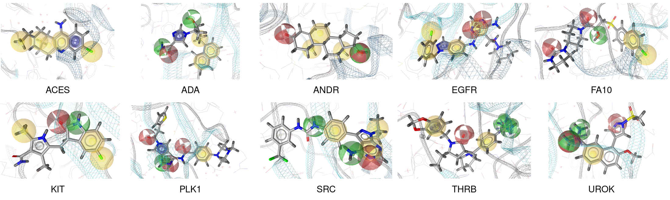
Figure A3: Structure-based pharmacophore queries of ten targets of the DUD-E benchmark dataset.

CDPKit alignment scoring function

The CDPKit implements alignment as a clique-detection algorithm and computes a rigid-body transformation via Kabsch’s algorithm to align the pharmacophore query $P_{Q}$ to the pharmacophore target $P_{T}$. The goodness of fit is evaluated with a geometric scoring function $S:\mathcal{P}\times\mathcal{P}\rightarrow\mathbb{R}_{+}$:

$$S(P_{Q},P_{T})=S_{MFP}(P_{Q},P_{T})+S_{Geom}(P_{Q},P_{T})$$ (14)

where $S_{MFP}:\mathcal{P}\times\mathcal{P}\rightarrow\mathbb{Z}_{+}$ counts the number of matched feature pairs and $S_{Geom}:\mathcal{P}\times\mathcal{P}\rightarrow[0,1)$ evaluates their geometric fit.

Runtime measurement

We measured alignment runtimes using the psdscreen tool from the CDPKit with 128 threads on an AMD EPYC 7713 64-Core Processor, while embedding and matching runtimes with PharmacoMatch were recorded using an NVIDIA GeForce RTX 3090 GPU with 24 GB GDDR6X. Runtime per pharmacophore was estimated by dividing the total runtime by the number of pharmacophores in each dataset, with the final estimate taken as the mean of ten runs. The results report the mean and standard deviation of these estimates across all ten datasets.

ROC curves

The performance metrics of our virtual screening experiments are derived from the ROC curves presented in Figures A4 and Figure A5.

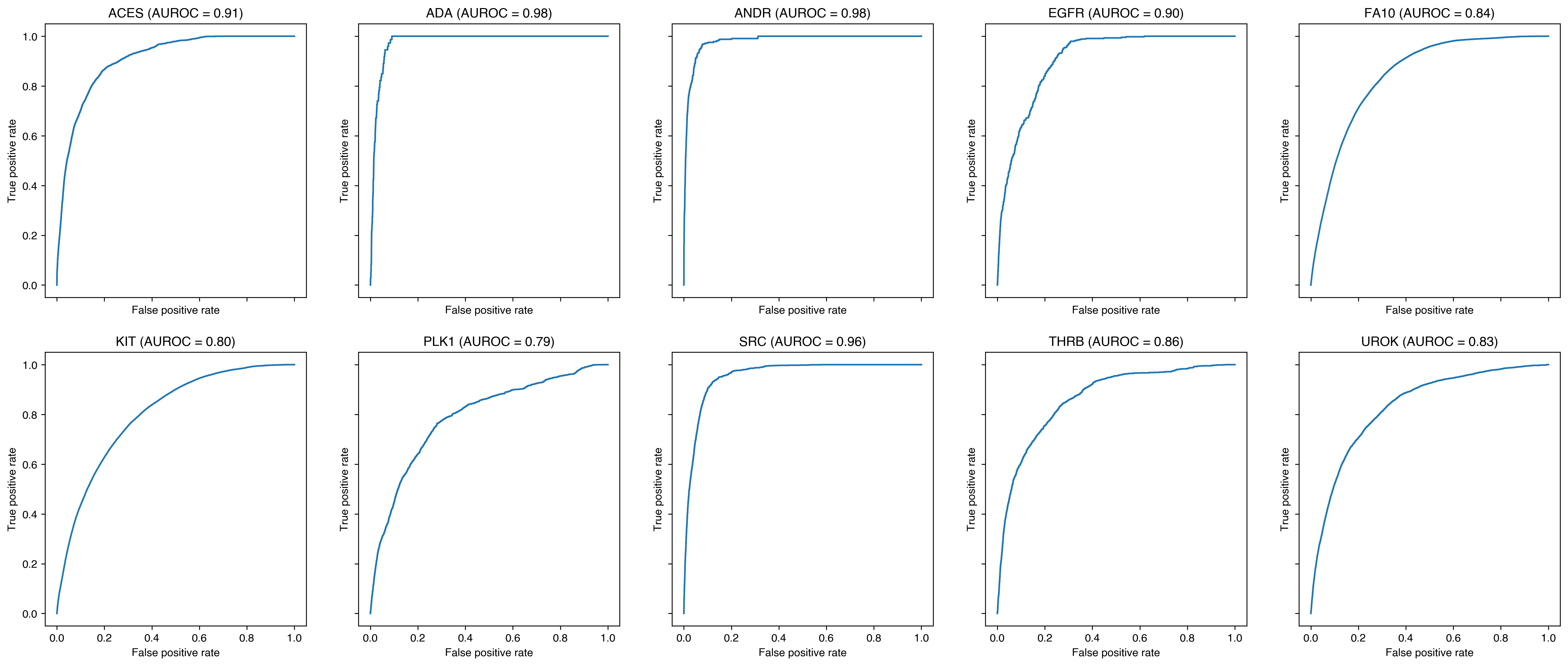
Figure A4: Performance comparison of PharmacoMatch and the alignment algorithm. The ROC-curves display the agreement of the hitlist ranking of the two algorithms for ten targets of the DUD-E benchmark dataset.

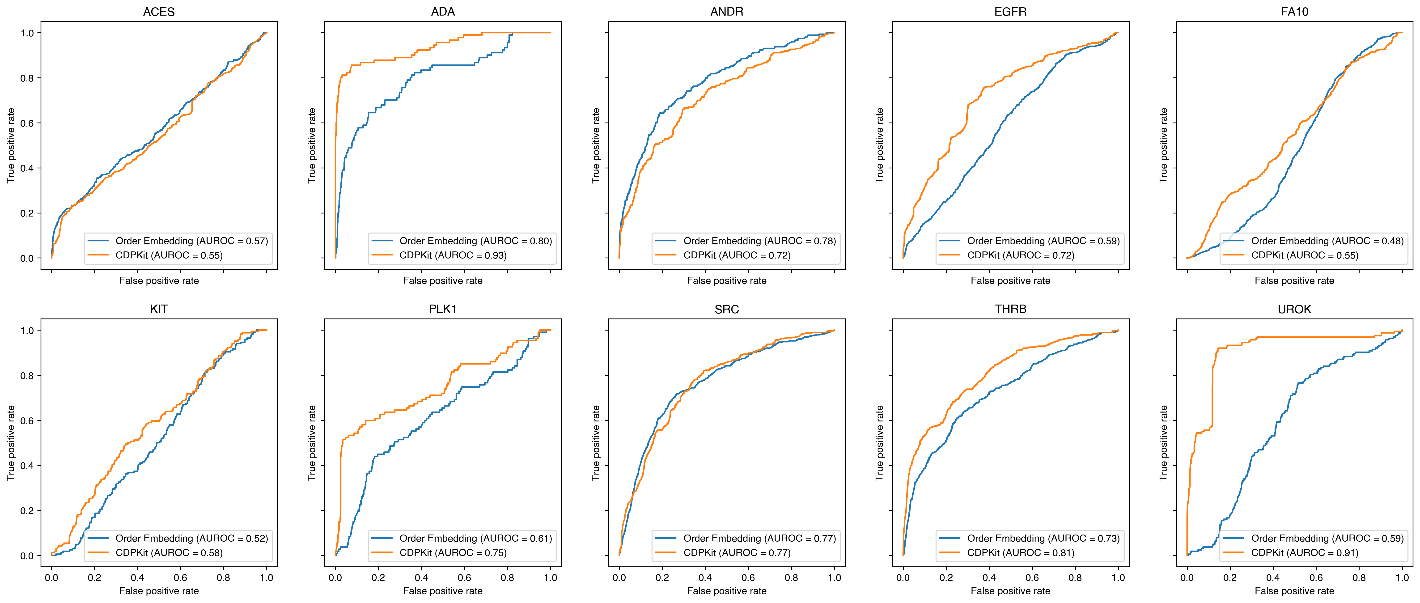
Figure A5: Absolute screening performance of PharmacoMatch and the alignment algorithm performance for ten targets of the DUD-E benchmark dataset. The pharmacophore queries were generated from the respective PDB ligand-receptor structures.

A.7 Embedding space visualization

UMAP visualization

UMAP embeddings for visualization plots were calculated with the UMAP Python library. The ‘metric‘ parameter was set to Manhattan distance, all other parameters are the default settings of the implementation. We tested a range of hyperparameters to ensure that the visualization results are not sensitive to parameter selection.

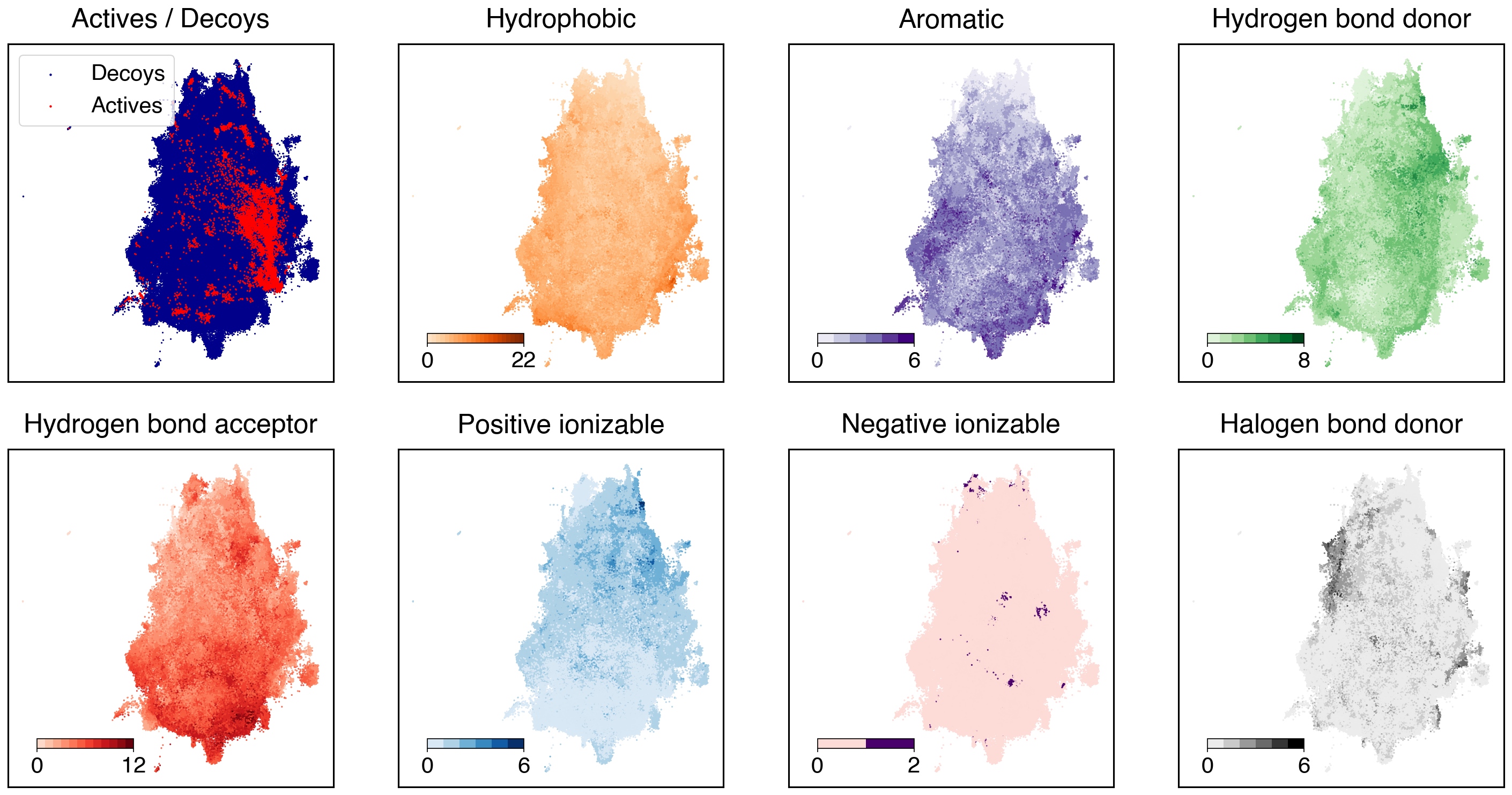
Figure A6: UMAP visualization of the vector embeddings of the ACES target.

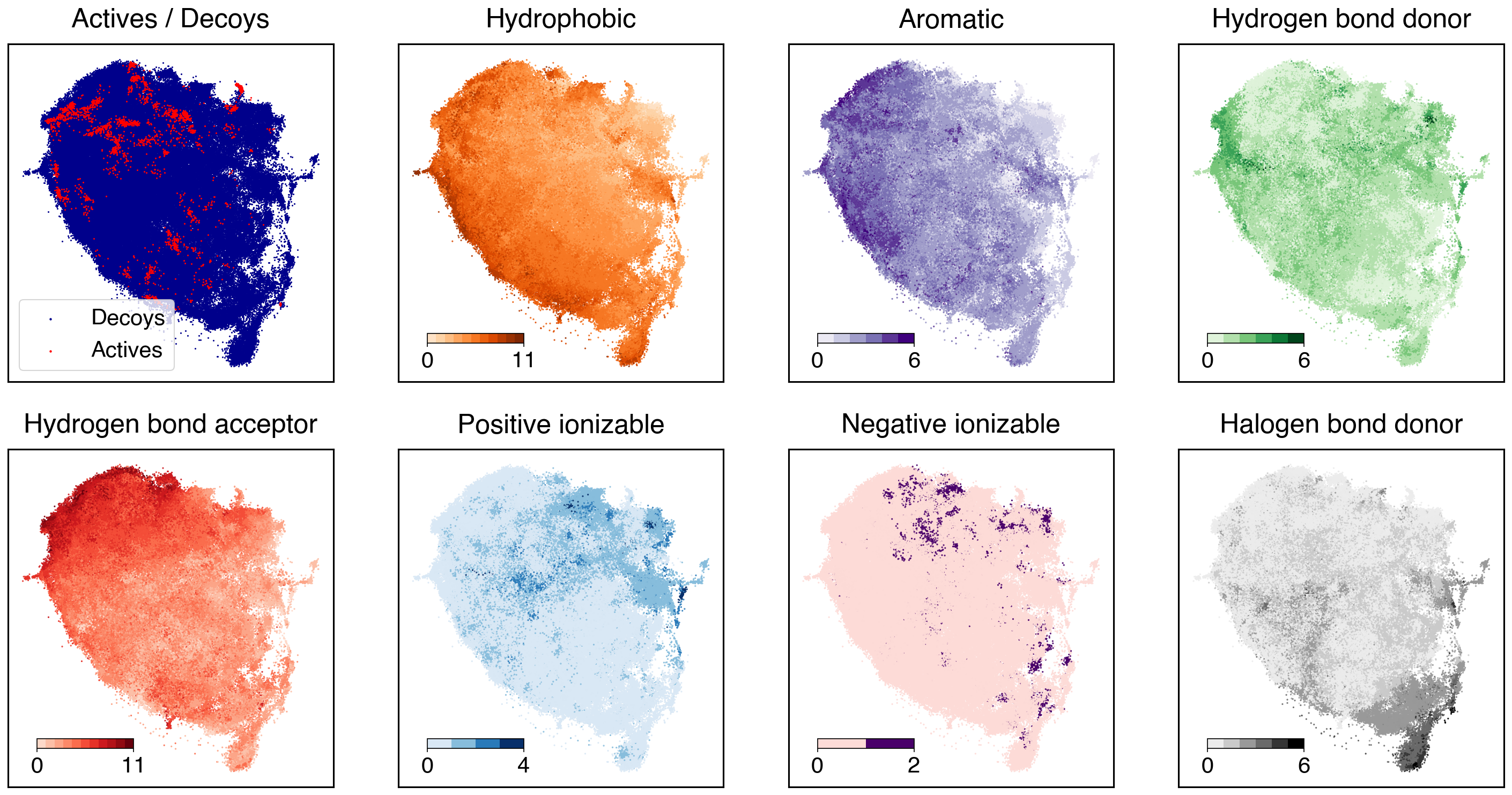
Figure A7: UMAP visualization of the vector embeddings of the ANDR target.

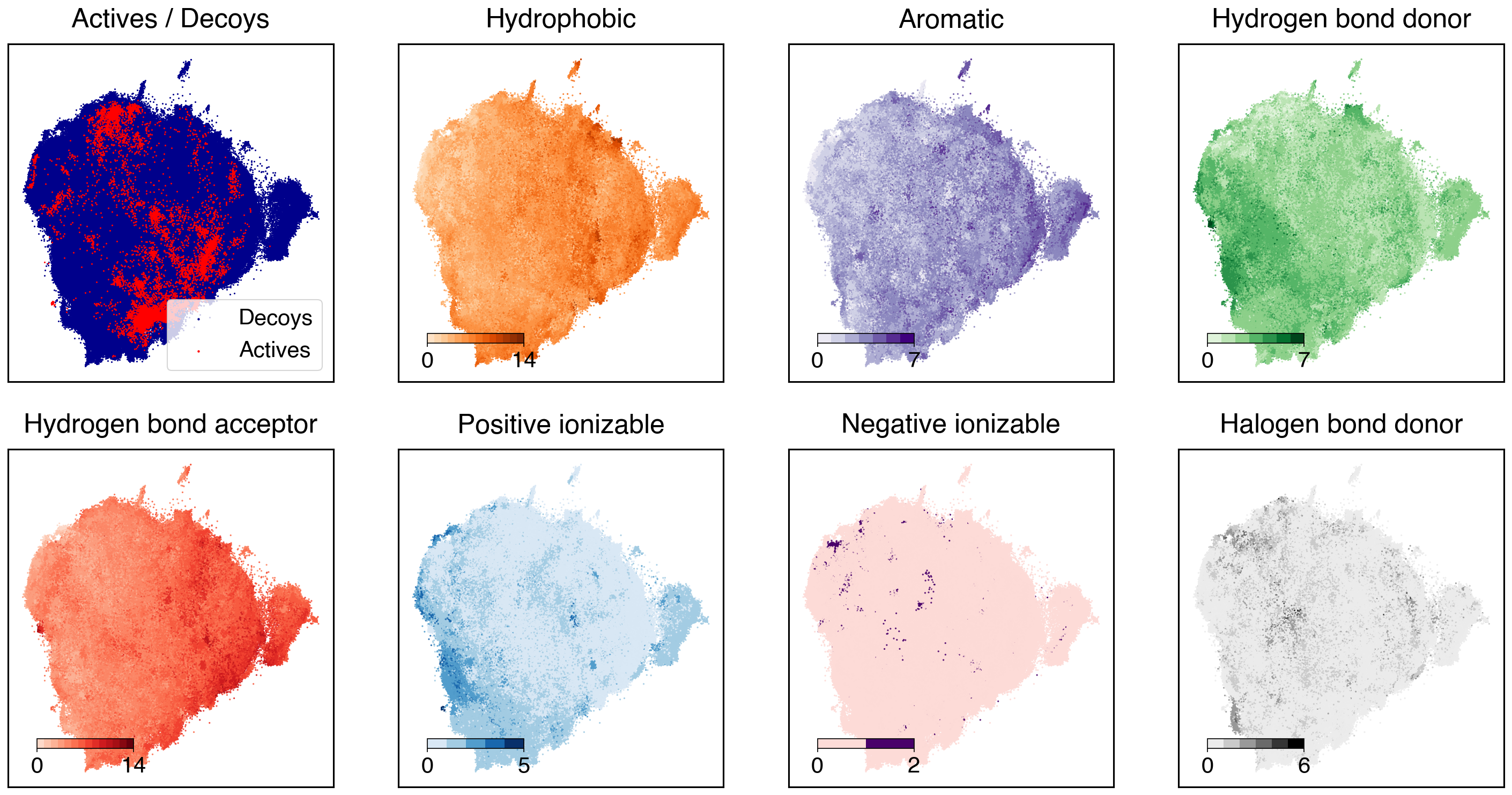
Figure A8: UMAP visualization of the vector embeddings of the EGFR target.

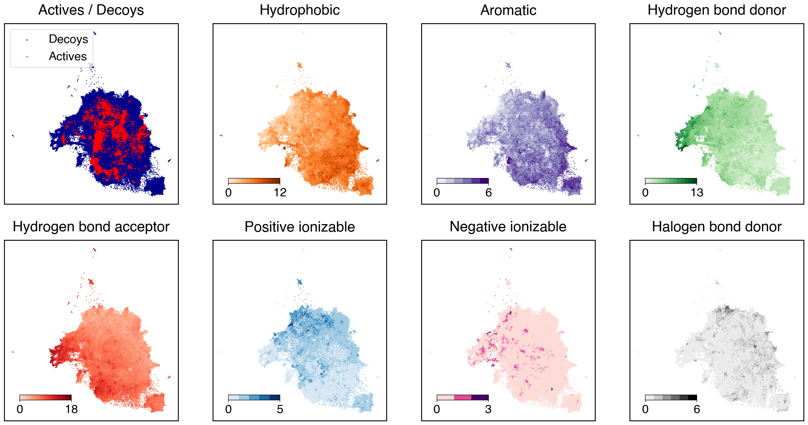
Figure A9: UMAP visualization of the vector embeddings of the FA10 target.

Figure A10: UMAP visualization of the vector embeddings of the KIT target.

Figure A11: UMAP visualization of the vector embeddings of the PLK1 target.

Figure A12: UMAP visualization of the vector embeddings of the SRC target.

Figure A13: UMAP visualization of the vector embeddings of the THRB target.

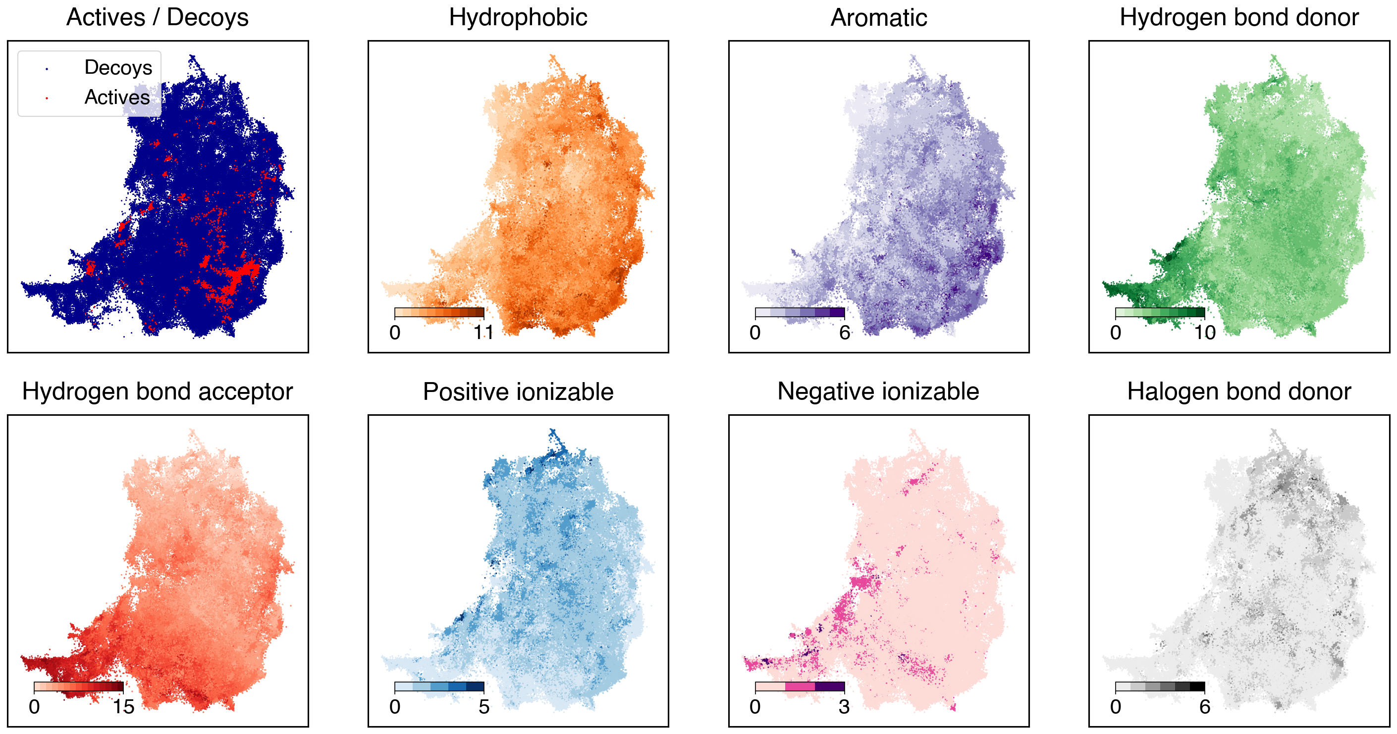
Figure A14: UMAP visualization of the vector embeddings of the UROK target.

References

- Balestriero et al. (2023) Balestriero, R.; Ibrahim, M.; Sobal, V.; Morcos, A.; Shekhar, S.; Goldstein, T.; Bordes, F.; Bardes, A.; Mialon, G.; Tian, Y.; Schwarzschild, A.; Wilson, A. G.; Geiping, J.; Garrido, Q.; Fernandez, P.; Bar, A.; Pirsiavash, H.; LeCun, Y.; and Goldblum, M. 2023. A Cookbook of Self-Supervised Learning. arXiv:2304.12210.
- Bengio, Courville, and Vincent (2013) Bengio, Y.; Courville, A.; and Vincent, P. 2013. Representation Learning: A Review and New Perspectives. IEEE Transactions on Pattern Analysis and Machine Intelligence, 35(8): 1798–1828.
- Burley et al. (2017) Burley, S. K.; Berman, H. M.; Kleywegt, G. J.; Markley, J. L.; Nakamura, H.; and Velankar, S. 2017. Protein Data Bank (PDB): the single global macromolecular structure archive. Protein crystallography: methods and protocols, 627–641.
- ChEMBL (2024) ChEMBL. 2024. ChEMBL Database - EMBL-EBI. https://www.ebi.ac.uk/chembl/. Accessed: 2024-01-06.
- Davies et al. (2015) Davies, M.; Nowotka, M.; Papadatos, G.; Dedman, N.; Gaulton, A.; Atkinson, F.; Bellis, L.; and Overington, J. P. 2015. ChEMBL web services: streamlining access to drug discovery data and utilities. Nucleic Acids Res., 43(W1): W612–W620.
- Dixon et al. (2006) Dixon, S. L.; Smondyrev, A. M.; Knoll, E. H.; Rao, S. N.; Shaw, D. E.; and Friesner, R. A. 2006. PHASE: a new engine for pharmacophore perception, 3D QSAR model development, and 3D database screening: 1. Methodology and preliminary results. J. Comput. Aided Mol. Des., 20: 647–671.
- Efron (1979) Efron, B. 1979. Bootstrap Methods: Another Look at the Jackknife. The Annals of Statistics, 7(1): 1 – 26.
- Falcon and The PyTorch Lightning team (2019) Falcon, W.; and The PyTorch Lightning team. 2019. PyTorch Lightning.
- Fey and Lenssen (2019) Fey, M.; and Lenssen, J. E. 2019. Fast Graph Representation Learning with PyTorch Geometric. arXiv:1903.02428.
- Gao et al. (2023) Gao, B.; Qiang, B.; Tan, H.; Jia, Y.; Ren, M.; Lu, M.; Liu, J.; Ma, W.-Y.; and Lan, Y. 2023. DrugCLIP: Contrastive Protein-Molecule Representation Learning for Virtual Screening. In Advances in Neural Information Processing Systems, volume 36, 44595–44614. Curran Associates, Inc.
- Gilmer et al. (2017) Gilmer, J.; Schoenholz, S. S.; Riley, P. F.; Vinyals, O.; and Dahl, G. E. 2017. Neural message passing for quantum chemistry. In International conference on machine learning, 1263–1272. PMLR.
- Hawkins, Skillman, and Nicholls (2007) Hawkins, P. C.; Skillman, A. G.; and Nicholls, A. 2007. Comparison of shape-matching and docking as virtual screening tools. J. Med. Chem., 50(1): 74–82.
- Huang et al. (2017) Huang, G.; Liu, Z.; Van Der Maaten, L.; and Weinberger, K. Q. 2017. Densely connected convolutional networks. In Proceedings of the IEEE conference on computer vision and pattern recognition, 4700–4708.
- Kabsch (1976) Kabsch, W. 1976. A solution for the best rotation to relate two sets of vectors. Acta Crystallographica Section A: Crystal Physics, Diffraction, Theoretical and General Crystallography, 32(5): 922–923.
- Kriege and Mutzel (2012) Kriege, N.; and Mutzel, P. 2012. Subgraph matching kernels for attributed graphs. In Proceedings of the 29th International Conference on Machine Learning, 291–298.
- Li et al. (2021) Li, H.; Sze, K.-H.; Lu, G.; and Ballester, P. J. 2021. Machine-learning scoring functions for structure-based virtual screening. Wiley Interdisciplinary Reviews: Computational Molecular Science, 11(1): e1478.
- Lipinski et al. (1997) Lipinski, C. A.; Lombardo, F.; Dominy, B. W.; and Feeney, P. J. 1997. Experimental and computational approaches to estimate solubility and permeability in drug discovery and development settings. Advanced Drug Delivery Reviews, 23(1): 3–25.
- Llanos et al. (2019) Llanos, E. J.; Leal, W.; Luu, D. H.; Jost, J.; Stadler, P. F.; and Restrepo, G. 2019. Exploration of the chemical space and its three historical regimes. Proceedings of the National Academy of Sciences, 116(26): 12660–12665.
- Mahé et al. (2006) Mahé, P.; Ralaivola, L.; Stoven, V.; and Vert, J.-P. 2006. The pharmacophore kernel for virtual screening with support vector machines. J. Chem. Inf. Model, 46(5): 2003–2014.
- McInnes, Healy, and Melville (2020) McInnes, L.; Healy, J.; and Melville, J. 2020. UMAP: Uniform Manifold Approximation and Projection for Dimension Reduction. arXiv:1802.03426.
- Mysinger et al. (2012) Mysinger, M. M.; Carchia, M.; Irwin, J. J.; and Shoichet, B. K. 2012. Directory of useful decoys, enhanced (DUD-E): better ligands and decoys for better benchmarking. J. Med. Chem., 55(14): 6582–6594.
- Permann, Seidel, and Langer (2021) Permann, C.; Seidel, T.; and Langer, T. 2021. Greedy 3-Point Search (G3PS)—A Novel Algorithm for Pharmacophore Alignment. Molecules, 26(23): 7201.
- Sadybekov et al. (2022) Sadybekov, A. A.; Sadybekov, A. V.; Liu, Y.; Iliopoulos-Tsoutsouvas, C.; Huang, X.-P.; Pickett, J.; Houser, B.; Patel, N.; Tran, N. K.; Tong, F.; et al. 2022. Synthon-based ligand discovery in virtual libraries of over 11 billion compounds. Nature, 601(7893): 452–459.
- Schütt et al. (2018) Schütt, K. T.; Sauceda, H. E.; Kindermans, P.-J.; Tkatchenko, A.; and Müller, K.-R. 2018. Schnet–a deep learning architecture for molecules and materials. J. Chem. Phys., 148(24).
- Seidel (2024) Seidel, T. 2024. Chemical Data Processing Toolkit source code repository. https://github.com/molinfo-vienna/CDPKit. Accessed: 2024-01-06.
- Seidel et al. (2017) Seidel, T.; Bryant, S. D.; Ibis, G.; Poli, G.; and Langer, T. 2017. 3D Pharmacophore Modeling Techniques in Computer-Aided Molecular Design Using LigandScout, chapter 20, 279–309. John Wiley & Sons, Ltd. ISBN 9781119161110.
- Seidel et al. (2010) Seidel, T.; Ibis, G.; Bendix, F.; and Wolber, G. 2010. Strategies for 3D pharmacophore-based virtual screening. Drug Discov. Today Technol., 7(4): e221–e228.
- Seidel et al. (2023) Seidel, T.; Permann, C.; Wieder, O.; Kohlbacher, S. M.; and Langer, T. 2023. High-quality conformer generation with CONFORGE: algorithm and performance assessment. J. Chem. Inf. Model, 63(17): 5549–5570.
- Sellner, Mahmoud, and Lill (2023) Sellner, M. S.; Mahmoud, A. H.; and Lill, M. A. 2023. Enhancing Ligand-Based Virtual Screening with 3D Shape Similarity via a Distance-Aware Transformer Model. bioRxiv:2023.11.17.567506.
- Seo and Kim (2023) Seo, S.; and Kim, W. Y. 2023. PharmacoNet: Accelerating Large-Scale Virtual Screening by Deep Pharmacophore Modeling. arXiv:2310.00681.
- Shivanyuk et al. (2007) Shivanyuk, A. N.; Ryabukhin, S. V.; Tolmachev, A.; Bogolyubsky, A.; Mykytenko, D.; Chupryna, A.; Heilman, W.; and Kostyuk, A. 2007. Enamine real database: Making chemical diversity real. Chemistry today, 25(6): 58–59.
- Simonovsky and Komodakis (2017) Simonovsky, M.; and Komodakis, N. 2017. Dynamic edge-conditioned filters in convolutional neural networks on graphs. In Proceedings of the IEEE conference on computer vision and pattern recognition, 3693–3702.
- Sliwoski et al. (2014) Sliwoski, G.; Kothiwale, S.; Meiler, J.; and Lowe, E. W. 2014. Computational methods in drug discovery. Pharmacological reviews, 66(1): 334–395.
- Taminau, Thijs, and De Winter (2008) Taminau, J.; Thijs, G.; and De Winter, H. 2008. Pharao: pharmacophore alignment and optimization. Journal of Molecular Graphics and Modelling, 27(2): 161–169.
- Truchon and Bayly (2007) Truchon, J.-F.; and Bayly, C. I. 2007. Evaluating virtual screening methods: good and bad metrics for the “early recognition” problem. J. Chem. Inf. Model, 47(2): 488–508.
- Virshup et al. (2013) Virshup, A. M.; Contreras-García, J.; Wipf, P.; Yang, W.; and Beratan, D. N. 2013. Stochastic voyages into uncharted chemical space produce a representative library of all possible drug-like compounds. J. Am. Chem. Soc., 135(19): 7296–7303.
- Warr et al. (2022) Warr, W. A.; Nicklaus, M. C.; Nicolaou, C. A.; and Rarey, M. 2022. Exploration of ultralarge compound collections for drug discovery. J. Chem. Inf. Model, 62(9): 2021–2034.
- Weininger (1988) Weininger, D. 1988. SMILES, a chemical language and information system. 1. Introduction to methodology and encoding rules. J. Chem. Inf. Comput., 28(1): 31–36.
- Wermuth et al. (1998) Wermuth, C.-G.; Ganellin, C.; Lindberg, P.; and Mitscher, L. 1998. Glossary of terms used in medicinal chemistry (IUPAC Recommendations 1998). Pure Appl. Chem., 70(5): 1129–1143.
- Wolber, Dornhofer, and Langer (2006) Wolber, G.; Dornhofer, A. A.; and Langer, T. 2006. Efficient overlay of small organic molecules using 3D pharmacophores. J. Comput. Aided Mol. Des., 20(12): 773–788.
- Wolber and Langer (2005) Wolber, G.; and Langer, T. 2005. LigandScout: 3-D pharmacophores derived from protein-bound ligands and their use as virtual screening filters. J. Chem. Inf. Model, 45(1): 160–169.
- Wolber et al. (2008) Wolber, G.; Seidel, T.; Bendix, F.; and Langer, T. 2008. Molecule-pharmacophore superpositioning and pattern matching in computational drug design. Drug Discov. Today, 13(1-2): 23–29.
- Ying et al. (2020) Ying, R.; Lou, Z.; You, J.; Wen, C.; Canedo, A.; and Leskovec, J. 2020. Neural Subgraph Matching. arXiv:2007.03092.
- Zdrazil et al. (2023) Zdrazil, B.; Felix, E.; Hunter, F.; Manners, E. J.; Blackshaw, J.; Corbett, S.; de Veij, M.; Ioannidis, H.; Lopez, D. M.; Mosquera, J.; Magarinos, M.; Bosc, N.; Arcila, R.; Kizilören, T.; Gaulton, A.; Bento, A.; Adasme, M.; Monecke, P.; Landrum, G.; and Leach, A. 2023. The ChEMBL Database in 2023: a drug discovery platform spanning multiple bioactivity data types and time periods. Nucleic Acids Res., 52(D1): D1180–D1192.