Measuring the ultrafast screening of $U$ in photo-excited charge-transfer insulators with time-resolved X-ray absorption spectroscopy

Abstract

Recent seminal experiments have utilized time-resolved X-ray absorption spectroscopy (XAS) to investigate the ultrafast photo-induced renormalization of the electron interaction (“Hubbard $U$”) in Mott and charge transfer insulators. In this paper, we analyze the change of interactions due to dynamical screening as it is encoded in the XAS signal, using the non-equilibrium GW+EDMFT formalism. Our study shows that XAS is well-suited for measuring this change, but two aspects should be kept in mind if the screening processes are not substantially faster than the valence electron dynamics: (i) Screening in a photo-excited system can affect both the position and the lineshape of the absorption lines. (ii) In general, the effect cannot be captured by the modification of a single interaction parameter. Specifically, an estimate for $\Delta U$ extracted from the shift of the XAS lines does not necessarily describe the related shift of the the upper Hubbard band. We clarify these aspects using a minimal cluster model and the three-band Emery model for a charge transfer insulator.

I Introduction

Due to its element selectivity, X-ray absorption spectroscopy (XAS) is a highly suitable probe of the local electronic structure in complex materials [1, 2, 3]. State-of-the-art X-ray free electron laser sources provide sufficient energy and time resolution to measure local multiplet energies on femtosecond timescales, which is useful to guide the engineering of functional material properties under non-equilibrium conditions [4, 5, 6, 7, 8]. In particular, XAS can potentially unravel photo-induced level shifts and elucidate the orbital nature of mobile carriers after “photo-doping”, i.e., a laser-induced transfer of electrons between different bands [9, 10, 11]. Photo-doping in Mott- or charge transfer insulators has been predicted to induce non-equilibrium phases ranging from hidden magnetic and orbital orders to superconductivity [7]. As is well-known from semiconductor studies [12], photo-doping can also modify the dielectric properties of a material, and therefore lead to a rapid screening of the electron interaction. In strongly correlated electron systems, this provides an intriguing possibility to control effective interaction parameters such as the local Hubbard interaction $U$ [13, 14, 15], with potentially profound impacts on the many-body state. Recently recorded shifts in the X-ray absorption spectrum of a photo-excited cuprate and nickelates can indeed be interpreted in terms of an ultrafast modification of $U$ [9, 11, 10], and similar shifts have been observed in photo-doped NiO [16].

The analysis of time-resolved XAS needs a robust theoretical modeling, because it relies on many relevant parameters, such as band shifts due to the interaction of electrons with photo-doped holes, and the core valence interaction. This has motivated microscopic theoretical descriptions of time-resolved XAS based on exact diagonalization [17, 9] and nonequilibrium Green’s functions [18]. In the present work, we will address a particular conceptual difficulty: Screening is not instantaneous. The photo-induced renormalization of the interaction originates from charge fluctuations which are activated by photo-doping, and which have energies comparable to the energy scales in the valence band. One therefore needs to clarify whether and how the dynamics of the screening process affects the XAS signal.

A theoretical description of screening in correlated electron systems can be achieved by combining the GW formalism [19] with extended dynamical mean-field theory (EDMFT) [20, 21, 22, 23, 24]. In this approach, similar to DMFT [25], the system is mapped to an impurity model which embeds one lattice site in a self-consistent environment that describes the rest of the lattice. In GW+EDMFT, this environment includes a fermion reservoir, with which the impurity can exchange electrons, and a spectrum of bosonic modes, which represent charge fluctuations in the lattice that can screen the local interaction. DMFT is well suited for calculating XAS spectra, because the core level can be added to the effective impurity model without changing the self-consistent environment [26, 27, 28, 29], also in the time-dependent case [18]. In the present work, we extend this idea to GW+EDMFT, in order to analyze how dynamic and static screening processes are reflected in time-resolved XAS.

The paper is structured as follows: In Sec. II we explain the evaluation of XAS within time-dependent GW+EDMFT simulations. In Sec. III, we demonstrate the effect of dynamical screening using a minimal model with a single bosonic mode to represent the charge fluctuations. Finally, in Sec. IV we discuss the photo-induced changes of the XAS spectrum within a model for a photo-doped charge transfer insulator. Sec. V provides a summary and further discussions.

II Evaluation of XAS within GW+EDMFT

II.1 General expression for the XAS signal

To calculate the X-ray absorption spectrum within the GW+EDMFT formalism, we closely follow the discussion in Ref. 18. We will first summarize the main aspects of the general formalism (without repeating the derivation), before discussing details relevant for GW+EDMFT in Sec. II.2 and II.3.

We start from a generic lattice model, with a set of valence and core orbitals at each lattice site $j$. The creation/annihilation operators for the valence and core electrons will be denoted by $d_{j,\alpha}$ ($d_{j,\alpha}^{\dagger}$) and $c_{j,\alpha}$ ($c_{j,\alpha}^{\dagger}$), respectively; Greek indices $\alpha$ label orbital and spin. For simplicity, the core-level Hamiltonian represents a single level with energy $\epsilon_{c}<0$,

$$H_{c}=\epsilon_{c}\sum_{j,\alpha}c_{j,\alpha}^{\dagger}c_{j,\alpha},$$ (1)

although more structure could be added [30, 31, 32, 28]. Within a semiclassical treatment of the incoming X-ray photon beam, a dipolar excitation from the core to the valence $d$-orbitals is described by the Hamiltonian

$$H_{\text{dip}}=g\big{(}s(t)e^{-\mathrm{i}\omega_{\text{in}}t}+h.c.\big{)}\sum_{j}\big{(}P_{j}+P_{j}^{\dagger}\big{)},$$ (2)

where $s(t)$ is the probe envelope, $\omega_{\text{in}}$ is the frequency of the incoming X-ray pulse, and $P_{j}^{\dagger}=\sum_{\alpha,\alpha^{\prime}}D_{\alpha,\alpha^{\prime}}\,d^{\dagger}_{j,\alpha}c_{j,\alpha^{\prime}}$ the dipolar transition operator, with the matrix element $D_{\alpha,\alpha^{\prime}}=\langle d,\alpha|\vec{r}\cdot\vec{\epsilon}|c,\alpha^{\prime}\rangle$ of the displacement operator ($\vec{r}$) projected onto the X-ray polarization direction $\vec{\epsilon}$. Due to the strong localization of the core orbital, we assume that the dipolar transition is between orbitals at the same site $j$ only. The prefactor $g$ sets the overall amplitude of the incoming probe pulse.

Because the X-ray photon energy $\omega_{\text{in}}$ is much larger than the energy of the valence electrons, we employ the rotating wave approximation and replace the dipolar transition (2) by

$$H_{\text{dip}}=g\sum_{j}\Big{(}s(t)e^{-\mathrm{i}\omega_{\text{in}}t}P_{j}^{\dagger}+h.c.\Big{)},$$ (3)

where terms $\sim e^{-\mathrm{i}\omega_{\text{in}}t}P_{j}$, which combine the emission of a photon and the creation of a core hole, are neglected. The X-ray signal is the fraction of absorbed photons during the pulse, or, in the semiclassical description, the ratio of the absorbed energy and the photon energy $\omega_{\text{in}}$. It is given by [18]

$$I_{\text{XAS}}=\lim_{g\to 0}\frac{1}{g^{2}}\sum_{j}\int dt\Big{[}\,gs(t)e^{-\mathrm{i}\omega_{\text{in}}t}\langle P_{j}^{\dagger}(t)\rangle-h.c.\Big{]}.$$ (4)

The limit $g\to 0$ indicates that the absorption is to be calculated to leading order in $g$, where the time-dependent expectation value $\langle P_{j}^{\dagger}(t)\rangle$ evaluated in the presence of the probe pulse (3) is of the order $\mathcal{O}(g)$. In the simulations, we explicitly evaluate the absorption signal $I_{\text{XAS}}$ with a nonzero probe pulse, and take the limit $g\to 0$ numerically.

An important observation is that Eq. (4) is a sum of local terms. One can therefore formally obtain the XAS signal by evaluating Eq. (4) with an effective action

$$S_{j}=S_{\text{loc}}+S_{\text{env}}$$ (5)

for site $j$, where $S_{\text{loc}}$ describes the dynamics generated by the local Hamiltonian $H_{\text{loc}}$ for the core and valence orbitals on site $j$, while $S_{\text{env}}$ describes the effect of the environment and is formally obtained by integrating out all degrees of freedom of the remaining lattice. Embedding techniques based on DMFT map the lattice model to a quantum impurity model which can reproduce the local correlation functions at a given site $j$, and thus yield an explicit expression for $S_{\text{env}}$. Because the XAS signal itself is already of order $\mathcal{O}(g^{2})$ in the probe amplitude $g$, one can to leading order in $g$ first determine the environment action $S_{\text{env}}$ in a simulation without the core levels, and then compute XAS in a post-processing step from an impurity model that has the same $S_{\text{env}}$, but is extended by the core level and the local part of the dipolar interaction (3).

II.2 GW+EDMFT

The valence electrons interact with a general density-density interaction,

$$H_{\text{int}}=\frac{1}{2}\sum_{j,j^{\prime}}\sum_{\alpha,\alpha^{\prime}}n_{d,j\alpha}v_{j-j^{\prime}}^{\alpha,\alpha^{\prime}}n_{d,j^{\prime}\alpha^{\prime}}.$$ (6)

Here $n_{d,j\alpha}=d_{j\alpha}^{\dagger}d_{j\alpha}$ is the local spin/orbital occupation number, $v_{j-j^{\prime}}$ denotes the bare interaction in real space, and $v_{\bm{q}}$ its Fourier transform (all interactions are understood as matrices in spin/orbital indices). The effect of screening is encoded in the fully screened interaction $W_{\bm{q}}(t,t^{\prime})$. The latter is the bare interaction reduced by the screening function (inverse dielectric function),

$$W_{\bm{q}}=\epsilon_{\bm{q}}^{-1}\ast v_{\bm{q}},$$ (7)

which in turn satisfies the exact relation

$$\epsilon_{\bm{q}}^{-1}=1-v_{\bm{q}}\ast\chi_{\bm{q}},$$ (8)

with the charge correlation function defined as $\chi_{\bm{q}}(t,t^{\prime})=-i\langle T_{\mathcal{C}}n_{d,\bm{q}}(t)n_{d,-\bm{q}}(t)\rangle$. Here and below, the functions are understood as matrices in spin/orbital indices, and for correlation functions, we use the two-time notation for Keldysh Green’s functions, following Ref. 33; $T_{\mathcal{C}}$ is the time ordering operator on the Keldysh contour. In equilibrium or in a steady state, the arguments $(t,t^{\prime})$ can be replaced by a single frequency. Products $A\ast B$ correspond to a convolution in time (product in frequency) and a matrix multiplication in the orbital indices.

Within the GW+EDMFT formalism, both the local Green’s function $G_{\text{loc}}=\frac{1}{N_{\bm{k}}}\sum_{\bm{k}}G_{\bm{k}}$ and the local fully screened interaction $W_{\text{loc}}=\frac{1}{N_{\bm{k}}}\sum_{\bm{k}}W_{\bm{k}}$ are obtained from a quantum impurity model. (All sites are equivalent due to translational invariance.) The impurity action is of the form of Eq. (5), with

$$S_{\text{env}}=S_{\Delta}+S_{\text{mf}}+S_{\mathcal{D}}.$$ (9)

Here $S_{\Delta}=-\sum_{\alpha\alpha^{\prime}}\int dtdt^{\prime}\,d_{\alpha}^{*}(t)\Delta_{\alpha,\alpha^{\prime}}(t,t^{\prime})d_{\alpha^{\prime}}(t^{\prime})\equiv-d^{\dagger}\ast\Delta\ast d$ describes the tunnelling of the valence electrons in and out of the lattice site $j$ via the hybridization function $\Delta$, and $S_{\text{mf}}$ is a mean-field potential for the electrons on site $j$ due to the static interaction with other sites (Hartree self energy). The last term is a retarded interaction

$$S_{\mathcal{D}}=-\frac{1}{2}\sum_{j,j^{\prime}}\sum_{\alpha,\alpha^{\prime}}\,n_{d,j\alpha}\ast\mathcal{D}\ast n_{d,\alpha^{\prime}j^{\prime}},$$ (10)

which represents a correction to the bare and instantaneous on-site interaction; we will denote the full dynamical impurity interaction by $\mathcal{U}=U+\mathcal{D}$. The functions $\Delta$ and $\mathcal{D}$ are determined through self-consistency relations, whose precise form is given in Ref. 13, 14. In particular, self-consistency enforces that the local fully screened interaction $W_{\text{loc}}$ matches the fully screened interaction $W_{\text{imp}}$ of the impurity model, which satisfies an equation $W_{\text{imp}}=\mathcal{U}-\mathcal{U}\ast\chi_{\text{imp}}\ast\mathcal{U}$ that is a local analog to Eqs. (7) and (8), with $\chi_{\text{imp}}$ the local charge susceptibility of the impurity model.

Within GW+EDMFT, the effect of screening can therefore be seen both in the fully screened interaction $W_{\text{imp}}=W_{\text{loc}}$, and in the effective impurity interaction $\mathcal{U}$. It should be emphasized, though, that neither quantity has the meaning of an effective Hubbard interaction in the lattice model. In particular, $\mathcal{U}$ is an auxiliary quantity used to characterize local correlation functions, and an impurity model with an effective interaction $\mathcal{U}$ does not imply that the system behaves like a Hubbard model with interaction $\mathcal{U}$ at every site.

II.3 XAS from GW+EDMFT

To obtain the XAS signal within the GW+EDMFT formalism, one first performs a time-dependent simulation without the core level. This fixes $\Delta$ and $\mathcal{U}$ of the impurity action. In a second step, one adds the core level and the dipolar excitation (3) to the local Hamiltonian, and computes the XAS signal from Eq. (4). The numerical computation of the XAS signal within an impurity model with retarded interaction still presents a formidable challenge. We use the strong coupling expansion approach of Ref. 22, which implements a double expansion in $\mathcal{D}$ and $\Delta$. For non-equilibrium steady-states, an exact evaluation of the strong-coupling expansion has recently been developed [34] and used in the context of non-equilibrium DMFT [35], but so far without retarded interactions. The development of a corresponding exact impurity solver for retarded interactions is beyond the scope of this work, and we restrict ourselves to the leading non-crossing approximation (NCA), as in previous GW+EDMFT studies [13, 14]. In part, the accuracy of this expansion will be assessed by comparison to the exactly solvable model of Sec. III.

The core hole has typically a short lifetime of a few femtoseconds, due to decay processes originating from Auger-Meitner decay [1]. Following previous theoretical works [26, 27, 28, 29, 18] we assume a near-exponential decay for the core hole, corresponding to a Lorentzian broadening of the XAS lines. In the real-time Keldysh formalism, the exponential decay of the core hole state can be introduced by attaching a wide-band particle reservoir to the core level, described by a core hybridization function $\Delta_{c}(t,t^{\prime})$ and an action analogous to $S_{\Delta}$. As in Ref. 18, we will use a Gaussian density of states for the core hybridization function $\Delta_{c}(\omega)=(\Gamma/\pi)\,e^{-(\omega/2W_{c})^{2}}$, which yields a simple analytic form for $\Delta_{c}(t,t^{\prime})$, and gives an exponential core-hole decay with a time constant $\Gamma^{-1}$ if the bandwidth $W_{c}$ is large.

III Minimal model

The screened interaction can be represented as arising from the coupling of the electron density to a bosonic field (Hubbard-Stratonovich field), whose spectrum is related to the charge fluctuations in the rest of the lattice. Before discussing the numerical results for charge-transfer insulators, we therefore consider a simple model which contains only a single harmonic screening mode. This model allows to illustrate the effect of the electron-boson coupling on the XAS signal on a qualitative level. The corresponding Hamiltonian reads

$$\begin{split}H=&\,\epsilon_{d}n_{d}+\epsilon_{c}n_{c}+Un_{d\uparrow}n_{d\downarrow}-\sqrt{2}\gamma\,\overline{n}_{d}X+\Omega_{0}b^{\dagger}b,\end{split}$$ (11)

where $b^{(\dagger)}$ annihilates (creates) a screening excitation with energy $\Omega_{0}$, and $\gamma$ describes the coupling between the electron density fluctuations $\overline{n}_{d}=n_{d\uparrow}+n_{d\downarrow}-1$ and the displacement $X=(b+b^{\dagger})/\sqrt{2}$ of the screening mode. The core and valence energy levels are $\epsilon_{c}$ and $\epsilon_{d}$, $U$ is the Hubbard repulsion in the valence orbital, and we choose $\epsilon_{d}=-U/2$ to enforce particle-hole symmetry. Any core-valence interaction is neglected as it will only produce an additional static energy shift on the absorption signal, because the model is purely local and the total electron density is preserved. In the initial state before the X-ray probe, the system is in the ground state with a single $d$-electron, and no screening mode is present.

The coupling between X-ray excited electrons and the screening mode gives rise to an additional, boson-mediated electronic interaction $\mathcal{D}$ on the $d$-orbital, which is obtained by integrating out the bosonic degrees of freedom in Eq. (11). This yields a contribution to the action analogous to Eq. (10), $S_{\mathcal{D}}=-\frac{1}{2}\,\bar{n}_{d}\ast\mathcal{D}\ast\bar{n}_{d}$, where the interaction

$$\mathcal{D}(t,t^{\prime}) =2\gamma^{2}\,D_{0}(t,t^{\prime}),$$ (12)

is determined by the boson propagator $D_{0}(t,t^{\prime})=-i\langle T_{\mathcal{C}}X(t)X(t^{\prime})\rangle$. In equilibrium, the retarded propagator becomes $D^{R}_{0}(\omega)=\Omega_{0}(\omega^{2}-\Omega_{0}^{2})^{-1}$, which results in the boson-mediated interaction

$$\mathcal{D}^{R}(\omega) =\frac{2\Omega_{0}\gamma^{2}}{\omega^{2}-\Omega_{0}^{2}}.$$ (13)

The real part of $\mathcal{D}^{R}(\omega)$ is shown in Fig. 1(a). The induced interaction approaches the value

$$\Delta U=-2\gamma^{2}/\Omega_{0}$$ (14)

at low frequencies ($\omega\rightarrow 0$), and becomes zero for $\omega\gg\Omega_{0}$. If the energy of the screening mode is larger than all relevant energy scales in the model (anti-adiabatic limit), screening mode excitations are suppressed and one can approximate $\mathcal{D}^{R}(\omega)$ by its static limit $\Delta U$. In this case the dominant effect of screening is to modify the Hubbard interaction $U$ into the screened interaction $U+\Delta U$. This analysis can be extended to investigate screening effects on XAS in more complex materials, where relevant screening modes have finite energy, as will be the case for the charge transfer insulator studied in Sec. IV.

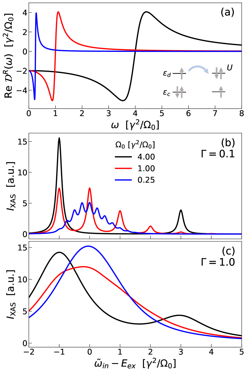
Figure 1: (a) Real part of the effective retarded interaction $\mathcal{D}^{R}(\omega+i0^{+})$ [Eq. (13)] for $\Omega_{0}=0.25,1,4$. All energies in this figure are measured in units of $\gamma^{2}/\Omega_{0}$. Divergences at $\Omega_{0}$ have been smoothened for a better visualization. The inset shows the X-ray absorption process. In addition to the doublon, for $\gamma\neq 0$, the final state can contain an arbitrary number $m$ of quanta in the screening mode. (b) and (c) XAS signal of the minimal model, Eq. (15). The inverse core-hole lifetime is $\Gamma=0.1$ (b) and $1.0$ (c).

Now we turn to the evaluation of the XAS signal in this minimal model. In the following, the photon energy is measured relative to the core level, $\omega_{\text{in}}=\tilde{\omega}_{\text{in}}+|\epsilon_{c}|$. For $\gamma=0$, there is a single X-ray absorption line at the energy corresponding to the transition shown in the inset of Fig. 1(a). This main absorption process corresponds to $\tilde{\omega}_{\text{in}}=U+\epsilon_{d}=\frac{U}{2}\equiv E_{\text{ex}}$, the excitonic resonance. For $\gamma\neq 0$, additional excitations of the screening mode alter the XAS spectrum and we evaluate the XAS signal (4) analytically, employing a Lang-Firsov transformation (details on the derivation can be found in Appendix A). For a long probe pulse ($s(t)\to 1$) one obtains

$$I_{\mathrm{XAS}}\propto\sum_{m=0}^{\infty}\frac{2\Gamma\cdot e^{-\gamma^{2}/\Omega_{0}^{2}}(\gamma/\Omega_{0})^{2m}/m!}{(\tilde{\omega}_{\text{in}}-E_{\text{ex}}+\gamma^{2}/\Omega_{0}-\Omega_{0}m)^{2}+\Gamma^{2}}.$$ (15)

The spectrum shows an infinite series of satellite peaks, corresponding to the excitation of one doublon and $m$ quanta $\Omega_{0}$ of the screening mode, each with a Lorentzian broadening due to the core-hole lifetime $1/\Gamma$. These boson satellites are analogous to sidebands in the optical absorption of molecules with well-defined vibrational modes. The lowest peak $(m=0)$ is centered at the bare transition energy $E_{\text{ex}}$, shifted by the value $\Delta U/2=-\gamma^{2}/\Omega_{0}$ due to the retarded interaction (14). The weights of the satellites follow a Poisson distribution with mean/standard deviation $\gamma^{2}/\Omega_{0}^{2}$.

The XAS signal (15) for various parameters $\gamma,\Omega_{0}$ is shown in Fig. 1(b)-(c), with $\gamma^{2}/\Omega_{0}$ as the unit of energy. One can identify two regimes, with distinct effects of the bosonic mode on the absorption spectrum: In the anti-adiabatic limit, $\Omega_{0}\gg\gamma$ ($\Omega_{0}=4$ in the figure), the dominant effect is the aforementioned redshift of the main peak, along with weak satellites at an offset $m\Omega_{0}$, i.e. far away from the excitonic resonance $E_{\text{ex}}$. In the adiabatic limit $\Omega_{0}\ll\gamma$, the dominant peak is no longer at $m=0$. Furthermore, due to the core-hole decay, the individual satellites broaden and merge into a single asymmetric line shape if $\Omega_{0}\lesssim\Gamma$ (see Fig. 1c). Thus, the superposition of many boson satellites appears as an additional broadening of the XAS absorption spectrum into an asymmetric peak. Because the weights of the satellites follow a Poisson distribution, the mean energy is at $\Omega_{0}\cdot\gamma^{2}/\Omega_{0}^{2}$, above the redshifted main absorption line, such that the mean position of this asymmetric line remains centered at the unscreened $\tilde{\omega}_{\text{in}}=E_{\text{ex}}$. For finite $\Gamma$ and in the ultra-adiabatic regime $\Omega_{0}\to 0$ ($\Omega_{0}=0.25$ in the figure), the XAS signal approaches again a symmetric (Gaussian) form centered around $\tilde{\omega}_{\text{in}}=E_{\text{ex}}$.

With these insights, it will be interesting to see whether the effect of the screening in typical charge transfer insulators also manifests itself in a modified lineshape. In addition to this qualitative discussion, the minimal model can serve as a benchmark for the approximate NCA impurity solver used in the remainder of the manuscript (see also the comment in Sec. II.3). It turns out that the NCA can reproduce the exact result (15) reasonably well in the adiabatic $\Omega_{0}\ll\gamma$ and anti-adiabatic $\Omega_{0}\gg\gamma$ regime, while for intermediate boson frequencies significant deviations can occur (see Appendix B for details).

IV XAS in charge-transfer insulators

IV.1 Model

We consider a two-dimensional three-band Emery model [36] on the square lattice with strongly interacting Cu orbitals, marked with an index $d$, and oxygen orbitals, marked with indices $p_{x}$ and $p_{y}$, as relevant for cuprate superconductors. The total Hamiltonian consist of the terms

$$H_{dp}=H_{\text{e}}+H_{\text{kin}}+H_{\text{int}},$$ (16)

$$H_{\text{e}}=\epsilon_{d}\sum_{i}n_{id}+\epsilon_{p}\sum_{i}(n_{ip_{x}}+n_{ip_{y}}),$$

$$H_{\text{kin}}=\sum_{ij\sigma}\sum_{\alpha,\beta}t_{ij}^{\alpha\beta}d_{i\alpha\sigma}^{\dagger}d_{j\beta\sigma},$$

where $d_{i\alpha\sigma}$ is the annihilation operator for unit cell $i$, orbital $\alpha\in\{d,p_{x},p_{y}\}$, and spin $\sigma$; $n_{i\alpha}=n_{i\alpha,\uparrow}+n_{i\alpha,\downarrow}$ is the corresponding density operator. The interaction is a density-density interaction of the general form (6), with $v_{i-j}^{\alpha\beta}=U$ if $i=j$ and $(\alpha;\beta)=(d\!\uparrow;d\!\downarrow)$ or $(d\!\downarrow;d\!\uparrow)$, and $v_{i-j}^{\alpha\beta}=U_{dp}$, when $(i\alpha)$ and $(j\beta)$ are nearest-neighbor $d$ and $p$ orbitals. The on-site energy of the $d$ orbital is given by $\epsilon_{d}$, and the crystal field splitting between the $d$ and $p$ orbitals $\Delta_{dp}=\epsilon_{p}-\epsilon_{d}$ is chosen such that the $p$ orbitals are completely filled, while the $d$ orbitals are singly occupied. The hopping between nearest neighbor $d$ and $p_{x}$, $p_{y}$ orbitals is denoted by $t_{dp}$ and between the $p_{x}$ and $p_{y}$ orbitals by $t_{pp}$.

In all calculations, we will fix the parameters to values relevant for La₂CuO₄, i.e., $U=5.0$ eV, $U_{dp}=2.0$ eV, $t_{dp}=0.5$ eV, $t_{dd}=-0.1$ eV, $t_{pp}=0.15$ eV and $\Delta_{pd}=-3.5$ eV; the inverse temperature is $\beta=5.0$ eV^-1. As the local interactions on the $d$ orbital are strongest, the EDMFT description is restricted to the $d$ orbitals only, while the $p$ orbitals are treated within the GW approximation. The same model has been studied within GW+EDMFT in Refs. 14, 13 in order to predict the photo-induced changes of the spectral function and the optical conductivity. Here we extend these studies to the XAS signal.

IV.2 Spectral function and screened interaction

For completeness, we will first reproduce from Ref. 14 the spectral properties of the $d$-$p$ subspace in equilibrium and after the photo-excitation. The spectral function is obtained from the two-time Green’s functions as $A(\omega,t)=-\frac{1}{\pi}\int_{t}^{t+t_{\text{cut}}}dt^{\prime}e^{\mathrm{i}\omega(t^{\prime}-t)}G^{R}(t^{\prime},t)$ with a cutoff time $t_{\text{cut}}=8$ fs both for the system with and without excitation. In Fig. 2(a), we show the spectral function in equilibrium and after photo-excitation. The almost fully occupied $p$ orbital is strongly hybridized with the lower Hubbard band of the $d$ orbital, forming three distinct features: The bonding Zhang-Rice band around $\omega=-1$ eV, a band of predominantly $p$ character around $\omega=-3$ eV, and the anti-bonding band at the highest binding energies. The unoccupied part of the spectrum is mainly composed of the $d$ orbital upper Hubbard band with a very small admixture of the $p$ orbital around $\omega=3$ eV. In the atomic limit, the position of the upper Hubbard band is

$$E_{\text{UHB}}=U+\epsilon_{d}.$$ (17)

To model the photo-excitation, the action of an electric field $\vec{E}(t)$ with polarization along the (11) direction is simulated. As found in Ref. 14, the excitation is followed by rapid intra-band relaxation processes on the timescale of a few femtoseconds, after which the system remains for a longer time in a non-thermal photo-doped state, whose properties are mainly controlled by the excitation density (photo-doping). The latter will be defined as the change $\Delta n_{d}$ in the $d$ occupancy. Because there are two $p$ orbitals and one $d$ orbital in each unit cell, there is a corresponding change $\Delta n_{p}=\tfrac{1}{2}\Delta n_{d}$ in the occupation per $p$ orbital ($\Delta n_{p}\equiv\Delta n_{p_{x}}=\Delta n_{p_{y}}$). In the present paper, we focus on the analysis of this photo-doped state, measured at the longest accessible time $t=12$ fs, rather than on the excitation process itself. Specifically, the field amplitude has a time profile

$$E(t)=E_{0}e^{-4.6(t-t_{0})^{2}/t_{0}^{2}}\sin(\Omega(t-t_{0})),$$ (18)

with a frequency $\Omega$ that is resonant with the charge transfer transition between the band with predominant $p$ character and the upper Hubbard band ($\Omega=6$ eV), and a duration $t_{0}=2\pi n/\Omega$ such that the envelope accommodates $n=4$ cycles. The field is coupled to the tight-binding model (16) using the Peierls substitution and a dipolar matrix element of magnitude $0.3ea$ ($e$ is the electronic charge and $a$ the lattice constant), see Ref. 14 for details. The amplitude $E_{0}$ of the electric field $\vec{E}(t)$ is adjusted to fix the amount of photo-doping.

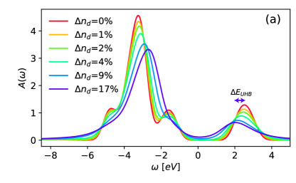
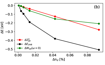
Figure 2: (a) Local spectral function in equilibrium (red line) and $t=12$ fs after the photo-excitation for various excitation densities $\Delta n_{d}$. $\Delta E_{\text{UHB}}$ indicates the shift of the upper Hubbard band upon photo-doping. (b) Hartree shift $\Delta\Sigma_{dd}^{H}$ [Eq. (19)], shift of the upper Hubbard band $\Delta E_{\text{UHB}}$, and change in the fully screened interaction $\Delta W_{dd}(0)/2$ (see main text) as a function of photo-doping $\Delta n_{d}$.

After the photo-excitation, the spectrum is modified in two characteristic ways, see Fig. 2(a). First, the bands are shifted toward the chemical potential, so that the bandgap is reduced. The analysis in Ref. 14 showed that the photo-induced bandgap renormalization originates from two effects: The redistribution of charges between the $d$ and $p$ orbitals leads to a mean-field potential on the $d$ band,

$$\Delta\Sigma^{H}_{dd}=\frac{U}{2}\Delta n_{d}-4U_{dp}\Delta n_{p}=\Big{(}\frac{U}{2}-2U_{dp}\Big{)}\Delta n_{d},$$ (19)

where the first factor $1/2$ is because the on-site Hubbard interaction acts only between electrons of different spin, and the factor $4$ counts the nearest-neighbor $p$ orbitals of a $d$ orbital. In a simpler Hartree Fock + DMFT (HF+DMFT) simulation, this mean field potential approximately explains the shift of the upper Hubbard band (Hartree shifts) [13, 14]. In the GW+EDMFT simulation, the shift $\Delta E_{\text{UHB}}$ of the upper Hubbard band is larger, indicating the effect of dynamical screening of the on-site Coulomb interaction. Both the Hartree shift and $\Delta E_{\text{UHB}}$ increase in magnitude with photo-doping, see Fig. 2(b). The second observation is that all bands are substantially broadened, which has been interpreted as a consequence of scattering of $d$ electrons on charge fluctuations [14, 13, 37]. At the largest excitations strengths, the broadening is so large that the fine structure in the occupied part of the spectrum is completely washed out.

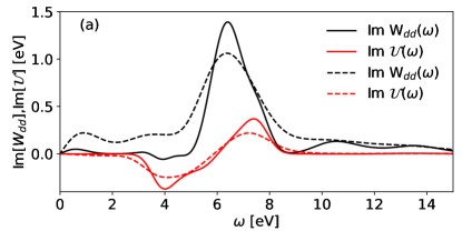
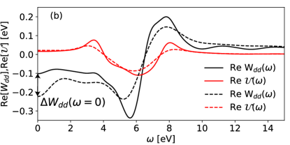
Figure 3: Imaginary (a) and real part (b) of the fully screened interaction $W_{dd}(\omega)$ and the effective impurity interaction $\mathcal{U}(\omega)$. Full lines show the equilibrium result, while dashed lines correspond to a photo-doped state with $\Delta n_{d}=4\%$ measured $t=12$ fs after the photo-excitation. $\Delta W_{dd}(\omega=0)$ marks the renormalization of the static interaction presented in Fig. 2.

Along with the photo-induced changes in the spectrum also the screening environment is substantially modified. In Fig. 3, we show the local fully screened interaction $W_{dd}(\omega,t)=\int_{t}^{t+t_{\text{cut}}}dt^{\prime}e^{\mathrm{i}\omega(t^{\prime}-t)}W^{R}_{dd}(t^{\prime},t)$ on the $d$-orbitals. In equilibrium, the spectrum $-\text{Im}W_{dd}(\omega)$ [Fig. 3(a)] shows a pronounced peak at the energy $\omega\approx 7$ eV, because screening processes are mainly associated with virtual charge fluctuations between the $p$ band and the upper Hubbard band. After the photo-excitation, additional spectral weight appears in $W_{dd}$ below $2$ eV, which is related to charge fluctuations of photo-doped doublons in the upper Hubbard band and holes in the Zhang-Rice band. Consequently, after the photo-doping, the real part $\text{Re}W_{dd}(\omega)$ [Fig. 3(a)] is suppressed below $\omega=1$ eV by an amount $\Delta W_{dd}(0)=\text{Re}W_{dd}(\omega=0)-\text{Re}W_{dd}(\omega=0)|_{\Delta n_{d}=0}$, which is another manifestation of dynamical screening. Assuming that the reduction of the effective interaction $\Delta W_{dd}(\omega=0)$ symmetrically modifies the gap size, we observe that $\Delta W_{dd}(\omega=0)/2$ and the Hartree shift each make a comparable contribution to the shift of the upper Hubbard band as the photodoping is increased [Fig. 2(b)].

The effective impurity interaction Im$\,\mathcal{U}(\omega)$ has a dip and peak structure with negative weight at positive frequencies already in equilibrium (Fig. 3(a)). The fact that $\text{Im}\,\mathcal{U}(\omega)$ can become negative in GW+EDMFT calculations is well known [38, 24, 39, 40]; while it does not necessarily imply a non-causal behavior in observable quantities, there are alternative formalisms of the self-consistency which enforce a positive spectral function of $\mathcal{U}(\omega)$ [41, 42]. Additionally, the combination of the NCA impurity solver with the GW+EDMFT can cause slight violations of causality [13]. Because $\mathcal{U}(\omega)$ is an auxiliary quantity within the present GW+EDMFT formalism, we will rely on observable quantities such as spectra and the fully screened interaction in the following discussion.

IV.3 XAS - Atomic limit

We will focus on the XAS signal of the strongly-interacting $d$ orbital, with a single core level,

$$H_{c}=\epsilon_{c}n_{c},$$ (20)

at energy $\epsilon_{c}<0$. In addition, there is typically a strong interaction between the core hole and the valence electrons,

$$H_{cd}=U_{cd}(n_{c}-2)n_{d},$$ (21)

defined such that the contribution vanishes for a system without core hole. Unless otherwise stated, we will consider the empirical relation $U_{cd}\approx 1.3U_{dd}=6.5$ eV, which has proven accurate for a broad range of transition metal oxides [43, 44, 29, 45]. The XAS signal in Eq. (4) is evaluated with a Gaussian probe envelope $s(t)$ of duration $\sigma=3.6$ fs. From now on, we will state the X-ray energies relative to the core energy, $\tilde{\omega}_{\text{in}}=\omega_{\text{in}}-|\epsilon_{c}|$.

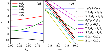
Figure 4: (a) Multiplet states of the cluster model (22), as the inter-cluster hopping is turned on ($t_{pp}$ is scaled along with $t_{pd}$). Groups of multiplets are labelled according to their dominant atomic configuration $m_{d}n_{p}$. Explicit expressions for the states are given in the App. C. (b) X-ray absorption will occur at $\tilde{\omega}_{\text{in}}=E_{a\to b}$, where the energies $E_{a\to b}$ are shown as a function of $U_{cd}$. The color and labelling of the lines only indicates from which group of multiplets the initial and final state of the X-ray transition is taken. The transition $1_{d}2_{p}\to\underline{2}_{d}2_{p}$ from the ground state configuration is shown in bold. The value for $U_{cd}$ used in the main text is $U_{cd}=6.5$ and $\tilde{t}_{dp}=1.0$.

.

Because the final states of the X-ray absorption process are often localized due to the strong core-valence interaction, it will be useful to support the interpretation of the numerical XAS spectra by a cluster model. Here, we introduce this cluster model and its multiplet states for later reference. We can start from a CuO₄ plaquette, i.e., one $d$-orbital in Eq. (16) with four surrounding $p$ orbitals. Due to to $C_{4}$ symmetry, only the symmetric (B_1g) combination of the four oxygen orbitals will hybridize with the copper $d_{x^{2}-y^{2}}$ orbital [46, 47, 48, 49, 50]. This leads to a model with one $d$ orbital and the symmetric $p$ orbital,

$$H=H_{\text{at}}+H_{c}+H_{cd}-\tilde{t}_{pd}\sum_{\sigma}(d_{\sigma}^{\dagger}p_{\sigma}+h.c.),$$ (22)

where

$$H_{\text{at}}=Un_{d\uparrow}n_{d\downarrow}+\tfrac{1}{2}U_{dp}n_{d}n_{p}+\epsilon_{d}n_{d}+\tilde{\epsilon}_{p}n_{p},$$ (23)

and the core contribution is given by Eqs. (20) and (21). The parameters $\tilde{\epsilon}_{p}=\epsilon_{p}-1.5t_{pp}$ and $\tilde{t}_{dp}=2t_{dp}$ are shifted with respect to the lattice Hamiltonian (16) due to the mapping on the symmetrized $p$ orbital. In principle, orthogonalization of orbitals on neighboring plaquettes would lead to a further small renormalization $\tilde{\epsilon}_{p}\rightarrow\epsilon_{p}-1.45t_{pp}$, $U_{dp}\rightarrow 0.92U_{dp}$ and $\tilde{t}_{dp}\rightarrow 1.92t_{dp}$ [49], but because we use the cluster model only for a qualitative comparison to the numerical data, we will neglect these shifts in the following.

In the atomic limit $t_{pd}=0$, multiplet states are simply given by integer occupancies, and will be denoted by $m_{d}n_{p}$, where $m\leavevmode\nobreak\ (n)\in\{0,1,2\}$ is the number of electrons on the $d$ ($p$) orbital. An underline as in $\underline{m}_{d}n_{p}$ will denote the state with an additional core hole. We will keep the same notation also for states with nonzero $t_{dp}.$ The initial state is therefore $1_{d}2_{p}$, and the XAS transition corresponds to $1_{d}2_{p}$ $\to$ $\underline{2}_{d}2_{p}$. For non-vanishing $t_{dp}$, one finds small shifts and splittings of the levels on the order O($t_{dp}^{2}/U_{dd}$,$t_{dp}^{2}/\Delta_{dp}$), see Fig. 4(a). For completeness, a detailed analysis of the states in such a cluster is presented in App. C. We will refer to the corresponding X-ray transition energies (Fig. 4(b)) in the following analysis of the numerical GW+EDMFT results.

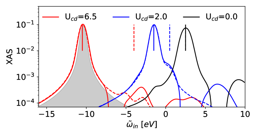
Figure 5: Equilibrium XAS as a function of the energy $\tilde{\omega}_{\text{in}}$ for different values of the core-valence interaction $U_{cd}$ calculated within GW+EDMFT. Dashed lines correspond to a Hartree-Fock + DMFT simulation, where the effect of dynamical screening is missing. The full vertical lines present the atomic estimate $E_{\text{ex}}$ of the exciton transition $1_{d}2_{p}\rightarrow\underline{2}_{d}2_{p}$ [Eq. (24)], and the dashed vertical lines mark the position $E_{\text{ex}}+U_{cd}$ of the continuum. The shaded region around $\tilde{\omega}_{\text{in}}=-10.5$ is a convolution of the probe pulse and the lifetime of the core hole rescaled to the height of the dominant peak, serving as an estimate of its lifetime.

IV.4 XAS - Equilibrium system

In equilibrium, the $d$ orbital is half-filled and the $p$ orbital is completely filled. In the atomic limit ($t_{pd}=0$), the dominant state is therefore $1_{d}2_{p}$, and the X-ray absorption corresponds to the transition $1_{d}2_{p}\rightarrow\underline{2}_{d}2_{p}$ at $\tilde{\omega}_{\text{in}}=E_{\text{ex}}$, with

$$E_{ex}=U+\epsilon_{d}-2U_{cd}=E_{\text{UHB}}-2U_{cd}.$$ (24)

(In the extended cluster model (22), with $\tilde{t}_{pd}=1.0$, the transition energy is only slightly shifted by $\Delta E=0.25$ eV.) Figure 5 shows the XAS spectrum obtained from the GW+EDMFT simulation in equilibrium. One indeed observes a main peak around energy $\tilde{\omega}_{\text{in}}=E_{\text{ex}}=-10.5$ eV. The final state $\underline{2}_{d}2_{p}$ is a local bound state (exciton), because the transfer of one $d$ electron of the local state $\underline{2}_{d}2_{p}$ to the continuum (i.e., to a different lattice site, leaving the configuration $\underline{1}_{d}2_{p}$ at the position of the core hole) would cost an energy $U_{cd}$ which exceeds the energy gain from delocalization. The line-shape of the main peak therefore well matches the convolution of a Lorentzian with inverse width $1/\Gamma=12$ fs due to the core hole decay and a Gaussian with width $\sigma=4$ fs due to the finite probe duration, see the dashed region in Fig. 5 and the discussion in Ref. 18. The missing data points around $\omega=-6$ eV and $-1$ eV correspond to regions of slightly negative spectral weight, which is a numerical artifact related to the non-causal effects discussed above and to the limited numerical accuracy.

Due to charge fluctuations in the initial state, the XAS transition can also lead to a final state in the continuum (local configuration $\underline{1}_{p}2_{p}$ with an additional $d$ electron in the rest of the lattice). In fact, we find a weak satellite to the main exciton at energy $\tilde{\omega}_{\text{in}}=E_{\text{ex}}+U_{cd}\approx-3$ eV (see dashed line). An alternative interpretation of this satellite could be a boson satellite due to the coupling to dynamic charge fluctuations. It is therefore instructive to compare the GW+EDMFT calculation with the HF+DMFT result, which does not include screening, see dashed-dotted line in Fig. 5. The comparison shows that the satellite signal, although overall weak, is enhanced if screening is taken into account, which shows that this peak is at least in part originating from charge fluctuations.

While in transition metal oxides there is typically a fixed relation between $U_{dd}$ and $U_{cd}$ [43, 44, 29], it is instructive to separate the two interactions by artificially adjusting $U_{cd},$ see Fig. 5. For $U_{cd}=2$ eV, the continuum forms a broad shoulder on top of the dominant resonance and the sidepeak due to bosonic excitations is now clearly present around $\omega-\omega_{\text{in}}=6$ eV. For $U_{cd}=0$, there is no formation of the exciton, but the sidepeak is clearly visible.

The fact that the bosonic satellite is rather weak for the present case can be rationalized with the minimal model of Sec. III, although it is clear that a comparison of the minimal model with the GW+EDMFT impurity model should not be over-interpreted. The two models can be related by the induced interaction, but one needs to take into account one subtle point: Because the charge susceptibility of an isolated site vanishes, the fully screened interaction $W_{dd}$ and the induced interaction (12) are identical in the minimal model (11). In contrast, $W_{\text{imp}}$ and $\mathcal{U}$ differ in the GW+EDMFT impurity model, because the hybridization between the impurity and bath leads to charge fluctuations on the $d$ orbital in the impurity model. The minimal model should be viewed as a toy model obtained from the GW+EDMFT impurity model after approximately eliminating the charge fluctuations from the environment, which will renormalize the fully screened interaction. We therefore link the two models by comparing the fully screened interaction $W_{dd}$ to the induced interaction (12), instead of the effective interaction $\mathcal{U}$. With this interpretation we match the parameters $\Omega_{0}$ and $2\gamma_{0}^{2}/\Omega_{0}$ in the minimal model with the position of the main peak in $\text{Im}W_{dd}(\omega)$ ($\Omega_{0}\approx 7$ eV) and the reduction $U-\text{Re}W_{dd}(\omega=0)\approx 0.1$ eV, respectively. This places the minimal model clearly in the anti-adiabatic regime, with $\gamma_{0}^{2}/\Omega_{0}^{2}=0.01$, which explains the very weak nature of the bosonic satellites in the XAS spectrum (in the anti-adiabatic limit, the first satellite in Eq. (15) is smaller than the main peak by a factor $\gamma_{0}^{2}/\Omega_{0}^{2}$).

IV.5 XAS - Photo-doped system

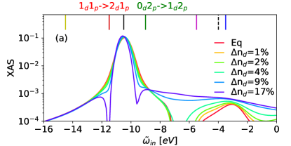
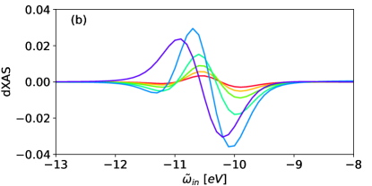
Figure 6: (a) XAS snapshot after the photoexcitation (pump-probe delay $12$ fs) for the indicated photodoping $\Delta n_{d}$. (b) Difference of the XAS signal with respect to the equilibrium signal (dXAS). The vertical lines in panel (a) indicate the X-ray transitions originating from excited initial states in the $p$-$d$ cluster at $U_{cd}=6.5$ eV and $\tilde{t}_{pd}=1.0$, using the same color code for the transitions as in Fig. 4(b). Selected transitions are labelled, such as the lowest transition from an initial state with a photo-doped $d$-hole ($0_{d}2_{p}$ $\to$ $\underline{1}_{d}2_{p}$) and with a photo-doped $p$-hole ($1_{d}1_{p}$ $\to$ $\underline{2}_{d}1_{p}$).

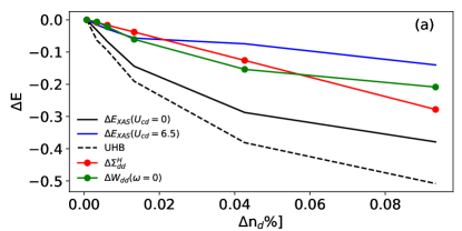
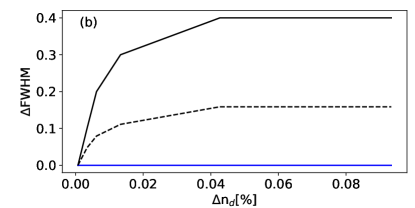
Figure 7: (a) Photoinduced shift in the excitonic energy versus the photodoping for $U_{cd}=6.5$ eV and $U_{cd}=0$ eV, compared to the shift of the upper Hubbard band (UHB), the Hartree shift $\Delta\Sigma^{H}_{dd}$ and the changes in the screening $\Delta W_{dd}/2$. (b) Change in the linewidth (FWHM) of the excitonic peak versus the photodoping $\Delta n$ (same labeling as in panel (a)). Here, the dashed line (UHB) indicates the change in the FWHM of the upper Hubbard band obtained from the local spectral function.

We will now analyze how the XAS signal is modified after a photo-excitation and what information can be extracted from these changes. We will focus on the physically relevant regime of strong core-valence interaction $U_{cd}=6.5$ eV and analyze the change in the spectrum as a function of the photodoping $\Delta n_{d}$, see Fig. 6. The dominant change in the spectrum is a shift of the exciton to larger binding energies, see also Fig. 6(b), which plots the difference with respect to equilibrium. Furthermore, additional spectral weight appears, mainly at smaller binding energies. Here, the dominant effect is the increase of the signal at the XAS continuum $\tilde{\omega}_{\text{in}}\approx-4$ in Fig. 6, which is expected as the photo-doping increases the number of mobile charge carriers.

First, we focus on the photo-induced shift $\Delta E_{\text{ex}}$ of the main exciton line. The maximum is determined by fitting a qubic spline and extracting the maxima from the interpolated curve. Figure 7(a) shows the shift as a function of the photo-doping $\Delta n_{d}$. Since the position of the peak in the atomic analysis is given by Eq. (24), the peak provides a first measure for the change in $U$. However, a closer analysis shows that there are two important facts one should keep in mind regarding this interpretation:

(i) In analogy to the shift of the upper Hubbard band discussed in Fig. 2(b), part of the shift can be explained by the Hartree shift (19) of the $d$ level. The red line in Fig. 7(a) shows the Hartree shift (same as in Fig. 2(b)). One can see that while the Hartree shift partially explains the renormalization of the exciton, the remaining shift nevertheless indicates a substantial contribution from dynamical screening and the renormalization of $U$.

(ii) With the shift of the XAS exciton and the upper Hubbard band, we now in principle have two independent experimental measures for the renormalization of the interaction, namely XAS and inverse photoemission spectroscopy [51] or two-photon photoemission [52, 53]. Comparing the expressions for the two quantities in the atomic limit (Eqs. (17) and (24)), one could expect that the two measures shift by the same amount if the effect of screening can be described by a simple renormalization of the Hubbard $U$. In contrast, by comparing $\Delta E_{\text{UHB}}$ and $\Delta E_{\text{XAS}}(U_{cd}=6.5)$ in Fig. 7(b), we see that the shift of the upper Hubbard band after photo-doping is substantially larger than the shift of the XAS exciton. (Because for $U_{cd}=0$, XAS is identical to electron addition up to core-hole lifetime effects, $\Delta E_{\text{UHB}}$ closely matches the shift $\Delta E_{\text{XAS}}(U_{cd}=0)$ for a simulation with $U_{cd}=0$, shown in Fig. 7(a).)

In part, the difference between $\Delta E_{\text{UHB}}$ and $\Delta E_{\text{ex}}$ is due to the fact that the change of the lineshape of the two spectral features upon photo-doping is substantially different (see Fig. 7(b)): While a strong broadening of the upper Hubbard band is observed, the line-width of the exciton changes only weakly. This difference is expected, as the delocalized states in the UHB induce a change in the electronic spectral function due to their scattering with photo-doped holes, in contrast to the localized exciton. The asymmetric broadening of the upper Hubbard band can also influence the determination of its mean-position. Beyond the different broadening of the exciton and the upper Hubbard band, a possible reason for the difference between $\Delta E_{\text{UHB}}$ and $\Delta E_{\text{ex}}$ is the combined effect of screening and charge fluctuations on the level shifts. In the minimal atomic model (11), which does not include any charge fluctuations on the impurity site, the effect of the screening mode on $E_{\text{UHB}}$ and $E_{\text{ex}}$ would indeed be identical. In the presence of the lattice, however, the final states with a doubly occupied impurity site are hybridized with unoccupied continuum states (in the GW+EDMFT impurity model, these appear as unoccupied spectral density in the hybridization function $\Delta$ around $\omega=E_{\text{UHB}}$). The hybridization shifts are smaller for the exciton, because continuum states are far off-resonant. Since the coupling to dynamic bosonic modes does not only modify the interaction, but also affects the tunnelling rate to the continuum, a different shift of $E_{\text{UHB}}$ and $E_{\text{ex}}$ is indeed expected.

Another issue to be discussed is the interaction between $p$ electrons and the core. So far, we have assumed that the core electrons interact only with the electrons at the same site, via the interaction $U_{cd}$, while for the valence orbitals, a nearest-neighbor interaction $U_{dp}$ is considered. More generally, we could introduce an oxygen-core interaction $U_{cp}$ as a free parameter in the Hamiltonian. Our assumption $U_{cp}=0$ is in line with the suggestion that there is a substantial asymmetry in the (nonlocal interactions of the core hole and valence $d$ electrons, based on the comparison of X-ray photoemission spectroscopy and optical conductivity data [54]. The opposite limit would be $U_{cp}=U_{dp}$, such that electrons on the $p$ orbitals interact with the charge on the entire copper atom (including core orbitals). Since the dominant XAS transition does not change the total charge on the copper atom, in contrast to electron addition spectroscopy, a nonzero $U_{cp}$ would give an additional asymmetry in the photo-induced shifts of the XAS lines and the electronic spectrum. For a full treatment of the case $U_{cp}\neq 0$ we would need to incorporate the $c$ level into the GW+EDMFT simulation, and also consider screened interactions $W_{cd}$.

In addition to the shift of the main exciton line, we observe additional spectral weight in the XAS spectrum (see in particular the curve for the large photo-doping $\Delta n_{d}=9\%$). Such changes can generally originate from two effects: First, photo-excitation opens new absorption channels, where the initial state corresponds to an electronically excited state. Analyzing these states in the $d$-$p$ cluster model (22), one finds that, depending on the interaction $U_{cd}$, many of the new transitions are nearly degenerate with the excitonic peak, see vertical lines in Fig. 6(a). Furthermore, we could again expect boson satellites due to the dynamical screening. Similar to the discussion in the equilibrium case (Sec. IV.4), one can try to estimate such boson satellites from the minimal model: After the photo-excitation, additional spectral weight appears in Im$\,W_{dd}$ around $\omega\approx\Omega_{0}=1$ eV (see Fig. 3). If, for a rough estimate, this weight is represented by an oscillator at $\Omega_{1}=1$ eV with a coupling $2\gamma_{1}^{2}/\Omega_{1}=\Delta W_{dd}(0)$, the system is still in the anti-adiabatic regime (e.g., $\Delta W_{dd}(0)\approx-0.1$ eV for $\Delta n_{d}=4\%$, such that $\gamma_{1}^{2}/\Omega_{1}^{2}=0.05$). Hence, for the photo-doped charge transfer insulator, we expect that these satellite features are still weak, such that at most the first side-peak may be visible. The latter, however, falls within the linewidth of the exciton. Both the additional XAS channels and the weak boson side-peaks will thus add up to a change of the lineshape of the main exciton. Indeed, the difference plot in Fig. 6(b) shows that the exciton is not only shifted. Due to the large intrinsic exciton linewidth, we cannot resolve the nature of the changes in the lineshape within the given accuracy. A possible perspective is to use resonant inelastic X-ray scattering (RIXS) to analyze charge fluctuations as these provide direct insights into excited bosonic spectrum.

V Conclusions

In conclusion, we have addressed how photoinduced changes in charge transfer insulators are encoded in the time-resolved XAS signal. In particular, after photodoping of charge-transfer insulators, bandgap renormalization is a well-established phenomenon observed in optical [55, 56, 57, 58] and photoemission [59] spectroscopy. Our work shows that XAS is also a sensitive measure of the dynamical renormalization of the Hubbard $U$, in line with the interpretation of recent experiments [9], and we analyzed in some detail how the screening is encoded in the time-resolved XAS signal.

One important conclusion is that different experimental probes of the interaction renormalization, like a measurement of the upper Hubbard band using inverse photoemission [51] or two-photon photoemission [52, 53], can respond differently to photo-induced changes in screening as compared to the excitonic XAS transitions. This should be contrasted to the response in the atomic limit, where both depend on $U$ in the same way. Our study therefore suggests that comparison between different spectroscopic probes for the dynamical screening in CT insulators will be very helpful for identifying the nature of photo-induced screening. Further, one should keep in mind that in multiorbital systems there are several mechanisms contributing to the band gap renormalization, in particular the retarded dynamical screening and the instantaneous Hartree shifts, which then depends on several microscopic parameters.

In principle, dynamical screening is also reflected both in a change of the position and the lineshape of the XAS exciton. We exemplified this using a minimal, exactly solvable model. In the adiabatic limit, the width of the XAS exciton does not only depend on the core hole lifetime, but also on the coupling and the frequency of the bosonic modes. In the anti-adiabatic limit, the main effects are excitonic redshifts and the build-up of side peaks at multiples of the bosonic energies. Compared with the full GW+EMDFT simulation, we find that for the CT insulator, the changes in the excitonic lineshapes are weak, because the screening modes have a frequency larger than the induced shifts (anti-adiabatic regime). Besides the screening modes, the XAS signal can also be modified through photo-activated transitions between cluster many-body states, leading to a shoulder-like structure at the excitonic edge and an enhancement of the continuum.

While the signal of the dynamical screening and photo-activated transitions in XAS is rather weak, RIXS might be a better tool to observe the boson sidepeaks. An extension of the formalism to RIXS [2, 17, 60, 61] would enable a direct analysis of photoinduced changes in screening modes. Previous studies of electron-lattice coupled systems with a single lattice mode [62] showed that one can separate the RIXS signal in photo-doped Mott insulators into the elastic electronic contribution and sidebands originating from the loss of energy to the lattice. A similar separation for the continuum of screening modes in charge transfer insulators would simplify the analysis and provide more direct insights into the origin of dynamical modification of Hubbard $U$ in realistic materials.

Our work also calls for improved formalisms for the treatment of screening and the calculation of the XAS signal. The GW+EDMFT formalism used in the present work can lead to a noncausal action, which could be avoided by a nonequilibrium extension of the modified GW+EDMFT formalism proposed in Refs. 41, 42. A further theoretical problem is the solution of the time-dependent impurity model, for which we employed the NCA approximation. A comparison with an exact solution of the atomic problem, see App. B, reveals substantial deviations if the system is away from the adiabatic or anti-adiabatic limit. These issues should be overcome by recent improvements in steady-state impurity solvers [34, 35] which need to be extended to include retarded density-density interactions.

Appendix A XAS for the minimal model

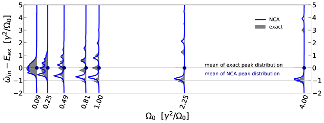
Figure 8: XAS signals for a single $d$-orbital, coupled to a harmonic screening mode according to Eqs. (15) and (29) in the exact ($T=0$) and NCA ($T=1/(50k_{B})$) description, respectively, for various screening frequencies $\Omega_{0}$. The unit of energy is set to $\gamma^{2}/\Omega_{0}$. The light gray line at $-\gamma^{2}/\Omega_{0}$ gives the static redshift induced by the presence of the harmonic screening mode. The dark gray line (blue dots) marks the mean of the XAS peak distribution according to the exact (NCA) calculation. The inverse core-hole lifetime is $\Gamma=0.1$.

In the following, we sketch the derivation of the XAS formula (15) for the minimal model (11). First, we set the dipole matrix elements to $D_{c\sigma,d\sigma^{\prime}}\equiv\delta_{\sigma,\sigma^{\prime}}$, such that the dipolar transition operator simplifies to $P^{\dagger}=\sum_{\sigma}d^{\dagger}_{\sigma}c_{\sigma}$. Second, for the minimal model, where the initial state $|\psi_{i}\rangle$ is an eigenstate (with energy $E_{i}=2\epsilon_{c}+\epsilon_{d}$) of the Hamiltonian $H$, we can modify the expression (4) for the XAS signal to yield

$$\begin{split}I_{\text{XAS}}=&\int dt_{1}\int dt_{2}\,s(t_{1})s(t_{2})\,e^{i(\omega_{\text{in}}+E_{i})(t_{2}-t_{1})}\\ &\quad\times\langle\psi_{i}|P\,e^{-iH(t_{2}-t_{1})}e^{-\Gamma|t_{2}-t_{1}|}P^{\dagger}|\psi_{i}\rangle,\end{split}$$ (25)

assuming a real-valued probe pulse envelope $s(t)$. This is a well-known expression for the XAS signal in a wavefunction-based description [17]. Furthermore, since the Hamiltonian (11) of the minimal model is time-independent, we will recover the equilibrium version of the XAS formula.

From now on we set $s(t)\equiv 1$, assuming an infinite X-ray probe window. Then, formally, expression (25) will diverge, however, the XAS rate, i.e. the measured number of photons per unit time, is finite. We will focus on the XAS rate for which only one integral over the time difference $\Delta t=t_{2}-t_{1}$ in expression (25) remains. In the final state after the X-ray absorption, additional screening modes will be excited due to the coupling $\propto\gamma\overline{n}_{d}X$. We calculate the energy of the final state by invoking a Lang-Firsov transform [63], which is a unitary transform with (anti-hermitian) generator $S=\frac{\gamma}{\Omega_{0}}\overline{n}_{d}(b-b^{\dagger})$. It transforms the Hamiltonian to $\tilde{H}=e^{S}He^{-S}=\epsilon_{d}n_{d}+\epsilon_{c}n_{c}+Un_{d\uparrow}n_{d\downarrow}+\Omega_{0}b^{\dagger}b-\frac{\gamma^{2}}{\Omega_{0}}\overline{n}_{d}^{2}$, thus removing the explicit electron-boson coupling. With this, the XAS rate becomes

$$I_{\text{XAS}}= \int d\Delta t\,e^{i(\omega_{\text{in}}+E_{i})\Delta t}e^{-\Gamma|\Delta t|}$$

$$\quad\times\langle\psi_{i}|Pe^{-S}e^{S}e^{-iH\Delta t}e^{-S}e^{S}P^{\dagger}|\psi_{i}\rangle$$

$$= \int d\Delta t\,e^{i(\omega_{\text{in}}+E_{i})\Delta t-\Gamma|\Delta t|}\langle\psi_{i}|Pe^{-S}e^{-i\tilde{H}\Delta t}e^{S}P^{\dagger}|\psi_{i}\rangle.$$ (26)

Expanding the X-ray excited state into energy eigenstates $|\tilde{\psi}_{f}\rangle$ of $\tilde{H}$ and performing the integral over $\Delta t$, one finds

$$I_{\text{XAS}}=\sum_{f}\frac{2\Gamma}{(\omega_{\text{in}}+E_{i}-\tilde{E}_{f})^{2}+\Gamma^{2}}\Big{|}\langle\psi_{i}|Pe^{-S}|\tilde{\psi}_{f}\rangle\Big{|}^{2}.$$ (27)

The electronic occupation of the initial and final states $|\psi_{i}\rangle,|\tilde{\psi}_{f}\rangle$ is fixed, hence the remaining degree of freedom to sum over in the final state is the screening mode excitation, i.e. the occupation of the bosonic state. If $|m\rangle_{\text{bos}}=\frac{\left(b^{\dagger}\right)^{m}}{\sqrt{m!}}|0\rangle_{\text{bos}}$ is the bosonic state with $m$ screening mode excitations, then the scalar product in (27) can be written as $\langle 0|e^{-(\gamma/\Omega_{0})(b-b^{\dagger})}|m\rangle_{\text{bos}}=(-\gamma/\Omega_{0})^{m}e^{-\gamma^{2}/2\Omega_{0}^{2}}/\sqrt{m!}$, which is the projection of a coherent state onto the $m$th occupation number state. Inserting this into the expression for $I_{\text{XAS}}$ above yields

$$I_{\text{XAS}}=\sum_{m=0}^{\infty}\frac{2\Gamma\cdot e^{-\gamma^{2}/\Omega_{0}^{2}}(\gamma/\Omega_{0})^{2m}/m!}{(\omega_{\text{in}}+\epsilon_{c}-\epsilon_{d}-U-\Omega_{0}m+\gamma^{2}/\Omega_{0})^{2}+\Gamma^{2}},$$ (28)

which is the XAS formula (15) in the main text.

Appendix B Harmonic screening within the non-crossing approximation

In this appendix we benchmark the non-crossing approximation (NCA) for a harmonic screening mode on the XAS spectrum. We show that in the adiabatic ($\Omega_{0}\ll\gamma$) and anti-adiabatic ($\Omega_{0}\gg\gamma$) limit the NCA reproduces the changes in the XAS signal (in terms of sidebands and excitonic peak shift) reasonably well.

To do so, we set up an impurity formulation of the harmonic screening model (11) which is obtained by integrating out the bosonic degrees of freedom, generating an effective interaction (12) for the electronic density fluctuations on the $d$-orbital. As discussed in Sec. III, the impurity action then takes the same form as in the full GW+EDMFT description, see Eqs. (5),(9) and (10), with vanishing hybridization and Hartree self energy on the $d$-orbital, $\Delta(t,t^{\prime})=0$ and $S_{\mathrm{mf}}=0$. The local Hamiltonian for $S_{\text{loc}}$ is $H_{\mathrm{loc}}=\epsilon_{d}n_{d}+\epsilon_{c}n_{c}+Un_{d,\uparrow}n_{d,\downarrow}$ and the effective interaction $\mathcal{D}(t,t^{\prime})$ is not selfconsistent but derived from the interaction with the screening mode,

$$\mathcal{D}(t,t^{\prime})=-2i\gamma^{2}\Omega_{0}\langle T_{\mathcal{C}}X(t)X(t^{\prime})\rangle,$$ (29)

c.f. Eq. (12). The NCA marks the leading order self-consistent expansion of physical observables in in $\mathcal{D}$, see Ref. 22. Otherwise, the XAS signal is evaluated as described in Sec. II.1, in particular Eq. (4), with constant dipole matrix elements $D_{c\sigma,d\sigma^{\prime}}\equiv\delta_{\sigma,\sigma^{\prime}}$ and a constant probe pulse envelope $s(t)\equiv 1$. A finite probe pulse envelope will further coarsen the spectral resolution of XAS, which we therefore ignore in this discussion in order to focus on the screening effects. One can further simplify the calculation by taking into account that, for the specific initial state with a singly occupied $d$-orbital, only the greater Keldysh component of $\mathcal{D}$ contributes in the strong-coupling hybridization expansion.

In Fig. 8, we show the XAS signal for different values of the screening frequency $\Omega_{0}$, while fixing the static redshift $\gamma^{2}/\Omega_{0}\equiv 1$, as obtained in the exact solution. The NCA results reproduce the broadening effect in the adiabatic ($\Omega_{0}\ll\gamma$) and the effective redshift in the anti-adiabtic ($\Omega_{0}\gg\gamma$) limit well. The mean of both peak distributions agrees for the entire parameter range. On the other hand, in the intermediate regime ($\Omega_{0}\sim\gamma$), neither the static redshift nor the position of the screening sidebands are reproduced correctly with the NCA. This suggests that in the adiabatic and anti-adiabatic regimes, we can extend the interpretation of screening effects on XAS in the minimal model (Sec. III) to the GW+EDMFT calculation presented in Section IV of this article.

Appendix C Cluster analysis

In this appendix, we provide further details on the atomic limit analysis. The solution of the whole cluster is not exactly solvable for any number of holes and therefore we will consider two cases where we can explicitely analyze all possible XAS transitions: a) the atomic limit with $t_{dd}=t_{dp}=t_{pp}=0$; b) a mapping of the CuO₄ cluster to a two-band model, which allows to analyze the effect of nonzero $t_{dp}$ and $t_{pp}$ by considering only the bonding combination of copper and oxygen orbitals.

First, we describe how to map the CuO₄ cluster to the two-band problem. We will retain only the symmetrized (B_1g) version of the oxygen orbitals, $p_{b}=(c_{p_{x+}}-c_{p_{y+}}-c_{p_{x-}}+c_{p_{y-}})/2$, as these hybridize with the copper $d_{x^{2}-y^{2}}$ orbital and neglect other symmetry sectors [46, 47, 48, 49, 50]. This leads to the Hamiltonian

$$\begin{split}H_{0}=&\epsilon_{d}n_{d}+\tilde{\epsilon}_{p}n_{p_{b}}+U_{dd}n_{d,\downarrow}n_{d,\uparrow}-\tilde{t}_{dp}\sum_{\sigma}(c_{d,\sigma}^{\dagger}c_{p_{b},\sigma}+h.c.)\\ &+U_{dp}/2n_{d}n_{p_{b}}+\tilde{\epsilon}_{c}n_{c}+U_{cd}n_{d}(n_{c}-2),\end{split}$$ (30)

where $\tilde{\epsilon}_{p}=\epsilon_{p}-1.5t_{pp}$ and $\tilde{t}_{dp}=2t_{dp}.$

Transition 1_d2_p $\rightarrow$ 2_d2_p.

In the atomic limit ($t_{dp}=t_{p}=0$), the energy of the transitions is given by $\omega=E_{\text{tot,at}}(\underline{2_{d}}2_{p},1)-E_{\text{tot,at}}(1_{d}2_{p},2)=U_{dd}/2-\epsilon_{c}-2U_{cd}.$ After the inclusion of the intercluster hopping $t_{dp}$, the transition is shifted to $\omega=E_{4,0,0}-E_{3,1/2,1/2}\approx U_{dd}/2-\epsilon_{c}-2U_{cd}+\left[4\frac{t_{dp}^{2}}{|U_{dd}/2-U_{dp}-\epsilon_{p}|}\right],$ where the square brackets emphasize the difference with respect to the atomic limit.

Transition 1_d1_p $\rightarrow$ 2_d1_p.

Similarly, the transition from 1_d1_p $\rightarrow\underline{2_{d}}1_{p}$ is in the atomic limit given by $\omega=E_{\text{tot,at}}(\underline{2_{d}}1_{p},1)-E_{\text{tot,at}}(1_{d}1_{p},2)=U_{dd}/2-\epsilon_{c}-2U_{cd}-U_{dp}/2.$ After the inclusion of the $t_{dp}$ hybridization, the transition is shifted to $\omega_{T}=E_{3,1/2,1/2}-E_{2,1,1}=E_{3,1/2,1/2}-E_{2,0,1}\approx U_{dd}/2-\epsilon_{c}-2U_{cd}-U_{dp}/2+\left[4\frac{t_{dp}^{2}}{|U_{dd}/2-U_{dp}-\epsilon_{p}|}\right]$. The main difference with respect to the previous transition is the shift by $-U_{dp}/2$ due to different occupation on the oxygen orbital. In the singlet channel, the transition is given by $\omega_{S}=E_{3,1/2,1/2}-E_{2,0,0}\approx U_{dd}/2-\epsilon_{c}-2U_{cd}-U_{dp}/2+\left[4\frac{t_{dp}^{2}}{|U_{dd}/2-U_{dp}-\epsilon_{p}|}+8\frac{t_{dp}^{2}}{|U_{dd}/2+\epsilon_{p}+U_{dp}|}-8\frac{t_{dp}^{2}}{|3U_{dd}/2+3U_{dp}/2+\epsilon_{p}|}\right]$.

0_d2_p $\rightarrow$ 1_d 2_p.

In the atomic limit of the main text, the energy of the transition is given by $\omega=E_{\text{tot,at}}(1_{d}2_{p},1)-E_{\text{tot,at}}(0_{d}2_{p},2)=-U_{dd}/2-\epsilon_{c}-U_{cd}$. In the cluster model, the transition is renormalized both due to the finite $d$-$p$ interaction and virtual hopping leads to the renormalized frequency $\omega=E_{3,1/2,1/2}-E_{2,0,0}=-U_{dd}/2-\epsilon_{c}-U_{cd}-4t_{dp}^{2}[\frac{1}{U_{dd}/2-U_{dp}-\epsilon_{p}}+\frac{2}{U_{dd}/2+3U_{dp}/2+\epsilon_{p}}].$

0d 1p $\rightarrow$ 0d 2p.

The atomic limit transition line is given by $\omega=E_{\text{tot,at}}(0_{d}2_{p},1)-E_{\text{tot,at}}(0_{d}1_{p},1)=\epsilon_{p}-\epsilon_{c}$. This line gets renormalized by the treatment of the whole cluster as $\omega=E_{2,0,0}-E_{1,1/2,1/2}=\epsilon_{p}-\epsilon_{c}-4\frac{t_{dp}^{2}}{U_{dd}/2+U_{dp}+\epsilon_{p}}+8\frac{t_{dp}^{2}}{U_{dd}/2+3U_{dp}/2+\epsilon_{p}}.$

1d 1p $\rightarrow$ 1d 2p.

In the atomic limit the transition is given by $\omega=E_{\text{tot,at}}(1_{d}2_{p})-E_{\text{tot,at}}(1_{d}1_{p})=\epsilon_{p}-\epsilon_{c}-U_{cd}+U_{dp}/2.$ Within the cluster two transition from the triplet state are degenerate $\omega_{T}=E_{3,1/2,1/2}-E_{2,1,1}=E_{3,1/2,1/2}-E_{2,0,1}=-\epsilon_{c}-U_{cd}+U_{dp}/2-4\frac{t_{dp}^{2}}{U_{dd}/2-U_{dp}-\epsilon_{p}}.$ The transition from the singlet state is $\omega_{S}=E_{3,1/2,1/2}-E_{2,0,0}=-\epsilon_{c}-U_{cd}+U_{dp}/2-4\frac{t_{dp}^{2}}{U_{dd}/2-U_{dp}-\epsilon_{p}}+8\frac{t_{dp}^{2}}{U_{dd}/2+U_{dp}+\epsilon_{p}}-8\frac{t_{dp}^{2}}{3U_{dd}/2+3U_{dp}/2+\epsilon_{p}}.$ As expected the induced splitting between the singlet and the triplet state is given by different second-order processes between the $d$ and $p$ orbital which for the given parameters are very small numbers and not accessible within the current numerical analysis.

0_d 2_p $\rightarrow$ 2_d 1_p.

The transition line in the atomic limit is given by $\omega=E_{\text{tot,at}}(2_{d}1_{p},2)-E_{\text{tot,at}}(0_{d}2_{p},1)=-\epsilon_{p}-U_{dp}-2U_{cd}-\epsilon_{c}$. The treatment of the whole $d$-$p$ cluster leads to the renormalization of the resonance as $\omega=E_{3,1/2,1/2}-E_{2,0,0}=-\epsilon_{p}-U_{dp}-2U_{cd}-\epsilon_{c}+4\frac{t_{dp}^{2}}{U_{dd}/2-U_{dp}-\epsilon_{p}}-8\frac{t_{dp}^{2}}{U_{dd}/2+3U_{dp}/2+\epsilon_{p}}.$

2d 1p $\rightarrow$ 2d 2p.

The transition line in the atomic limit is given by $\omega=E_{\text{tot,at}}(2_{d}2_{p})-E_{\text{tot,at}}(2_{d}1_{p})=-\epsilon_{c}+\epsilon_{p}+U_{dp}-2U_{cd}$. The treatment of the whole $d$-$p$ cluster leads to the renormalization of the resonance as $\omega=E_{4,0,0}-E_{3,1/2,1/2}=-\epsilon_{c}+\epsilon_{p}+U_{dp}-2U_{cd}-4\frac{t_{dp}^{2}}{U_{dd}/2-U_{dp}-\epsilon_{p}}$.

$\alpha\leavevmode\nobreak\ (N,S_{z},S))$	$|j\rangle\in\alpha$	$E_{\alpha}$
$(0,0,0)$	$|0,0\rangle$	0
$(1,1/2,1/2)$	$\{|\uparrow,0\rangle$, $|0,\uparrow\rangle$}	$\frac{(-U_{dd}/2-U_{dp}+\epsilon_{p})}{2}\pm\sqrt{\left(\frac{U_{dd}/2+U_{dp}+\epsilon_{p}}{2}\right)^{2}+4t_{dp}^{2}}$
$(2,1,1)$	$|\uparrow,\uparrow\rangle$	$-U_{dd}/2+\epsilon_{p}-U_{dp}/2$
$(2,0,0)$	$\{|\!\uparrow\downarrow,0\rangle$,$|0,\uparrow\downarrow\rangle$ $,|\!\downarrow,\uparrow\rangle-|\!\uparrow,\downarrow\rangle$}	$-\frac{8t_{dp}^{2}}{-U_{dd}/2-3U_{dp}/2-\epsilon_{p}}+2\epsilon_{p}$ $-U_{dd}/2-U_{dp}/2+\epsilon_{p}-\frac{8t_{dp}^{2}}{\epsilon_{p}+U_{dd}+U_{dp}}+\frac{8t_{dp}^{2}}{\epsilon_{p}+3U_{dd}/2+3U_{dp}/2}$ $-2U_{dp}-\frac{8t_{dp}^{2}}{\epsilon_{p}+3(U_{dd}+U_{dp})/2}$
$(2,0,1)$	$\{|\!\downarrow,\uparrow\rangle+|\!\uparrow,\downarrow\rangle$}	$-U_{dd}/2+\epsilon_{p}-U_{dp}/2$
$(3,1/2,1/2)$	$\{|\!\uparrow,\uparrow\downarrow\rangle$, $|\!\uparrow\downarrow,\uparrow\rangle$}	$\frac{(-U_{dd}/2-U_{dp}+3\epsilon_{p})}{2}\pm\sqrt{\left(\frac{U_{dd}/2-U_{dp}-\epsilon_{p}}{2}\right)^{2}+4t_{dp}^{2}}$
$(4,0,0)$	$|\!\uparrow\downarrow,\uparrow\downarrow\rangle$	$2\epsilon_{p}$

Table 1: Labeling of states in the $d$-$p$ cluster, where states are sorted by the total number of electrons $N$, $z$-component of the total spin $S_{z}$ and the total spin $S$. For states with a nonzero value of $S_{z}$ we show only fully polarized states. The second column shows the $d$-$p$ states belonging to a given multiplet $\alpha$, where the first (second) entry in the ket refers to the hole occupation of orbital $d$ ($p_{+}$). The last column shows the energy of the states except for (N,S_z,S)=(2,0,0), where the analytical expressions are too complicated, and energies are calculated within second order perturbation theory.

References

- de Groot et al. [2021] F. M. de Groot, H. Elnaggar, F. Frati, R.-p. Wang, M. U. Delgado-Jaime, M. van Veenendaal, J. Fernandez-Rodriguez, M. W. Haverkort, R. J. Green, G. van der Laan, et al., 2p x-ray absorption spectroscopy of 3d transition metal systems, Journal of Electron Spectroscopy and Related Phenomena 249, 147061 (2021).
- Ament et al. [2011] L. J. P. Ament, M. van Veenendaal, T. P. Devereaux, J. P. Hill, and J. van den Brink, Resonant inelastic x-ray scattering studies of elementary excitations, Rev. Mod. Phys. 83, 705 (2011).
- Kuo et al. [2017] C. Y. Kuo, T. Haupricht, J. Weinen, H. Wu, K. D. Tsuei, M. Haverkort, A. Tanaka, and L. Tjeng, Challenges from experiment: electronic structure of nio, The European Physical Journal Special Topics 226, 2445 (2017).
- Giannetti et al. [2016] C. Giannetti, M. Capone, D. Fausti, M. Fabrizio, F. Parmigiani, and D. Mihailovic, Ultrafast optical spectroscopy of strongly correlated materials and high-temperature superconductors: a non-equilibrium approach, Adv. Phys. 65, 58 (2016).
- Basov et al. [2017] D. N. Basov, R. D. Averitt, and D. Hsieh, Towards properties on demand in quantum materials, Nature Materials 16, 1077 (2017).
- de la Torre et al. [2021] A. de la Torre, D. M. Kennes, M. Claassen, S. Gerber, J. W. McIver, and M. A. Sentef, Colloquium: Nonthermal pathways to ultrafast control in quantum materials, Rev. Mod. Phys. 93, 041002 (2021).
- Murakami et al. [2023] Y. Murakami, D. Golež, M. Eckstein, and P. Werner, Photo-induced nonequilibrium states in Mott insulators (2023), arXiv:2310.05201 [cond-mat.str-el] .
- Boschini et al. [2024] F. Boschini, M. Zonno, and A. Damascelli, Time-resolved arpes studies of quantum materials, Rev. Mod. Phys. 96, 015003 (2024).
- Baykusheva et al. [2022] D. R. Baykusheva, H. Jang, A. A. Husain, S. Lee, S. F. R. TenHuisen, P. Zhou, S. Park, H. Kim, J.-K. Kim, H.-D. Kim, M. Kim, S.-Y. Park, P. Abbamonte, B. J. Kim, G. D. Gu, Y. Wang, and M. Mitrano, Ultrafast renormalization of the on-site coulomb repulsion in a cuprate superconductor, Phys. Rev. X 12, 011013 (2022).
- Wang et al. [2022] X. Wang, R. Y. Engel, I. Vaskivskyi, D. Turenne, V. Shokeen, A. Yaroslavtsev, O. Grånäs, R. Knut, J. O. Schunck, S. Dziarzhytski, et al., Ultrafast manipulation of the nio antiferromagnetic order via sub-gap optical excitation, Faraday discussions 237, 300 (2022).
- Grånäs et al. [2022] O. Grånäs, I. Vaskivskyi, X. Wang, P. Thunström, S. Ghimire, R. Knut, J. Söderström, L. Kjellsson, D. Turenne, R. Engel, et al., Ultrafast modification of the electronic structure of a correlated insulator, Physical Review Research 4, L032030 (2022).
- Huber et al. [2001] R. Huber, F. Tauser, A. Brodschelm, M. Bichler, G. Abstreiter, and A. Leitenstorfer, How many-particle interactions develop after ultrafast excitation of an electron–hole plasma, Nature 414, 286 (2001).
- Golež et al. [2019a] D. Golež, L. Boehnke, M. Eckstein, and P. Werner, Dynamics of photodoped charge transfer insulators, Phys. Rev. B 100, 041111 (2019a).
- Golež et al. [2019b] D. Golež, M. Eckstein, and P. Werner, Multiband nonequilibrium formalism for correlated insulators, Phys. Rev. B 100, 235117 (2019b).
- Tancogne-Dejean et al. [2018] N. Tancogne-Dejean, M. A. Sentef, and A. Rubio, Ultrafast modification of hubbard in a strongly correlated material: Ab initio high-harmonic generation in nio, Phys. Rev. Lett. 121, 097402 (2018).
- Lojewski et al. [2024] T. Lojewski, D. Golez, K. Ollefs, L. L. Guyader, L. Kämmerer, N. Rothenbach, R. Y. Engel, P. S. Miedema, M. Beye, G. S. Chiuzbăian, R. Carley, R. Gort, B. E. V. Kuiken, G. Mercurio, J. Schlappa, A. Yaroslavtsev, A. Scherz, F. Döring, C. David, H. Wende, U. Bovensiepen, M. Eckstein, P. Werner, and A. Eschenlohr, Photo-induced charge-transfer renormalization in nio (2024), arXiv:2305.10145 [cond-mat.str-el] .
- Chen et al. [2019] Y. Chen, Y. Wang, C. Jia, B. Moritz, A. M. Shvaika, J. K. Freericks, and T. P. Devereaux, Theory for time-resolved resonant inelastic x-ray scattering, Phys. Rev. B 99, 104306 (2019).
- Werner et al. [2022] P. Werner, D. Golez, and M. Eckstein, Local interpretation of time-resolved x-ray absorption in mott insulators: Insights from nonequilibrium dynamical mean-field theory, Phys. Rev. B 106, 165106 (2022).
- Hedin [1965] L. Hedin, New method for calculating the one-particle green’s function with application to the electron-gas problem, Phys. Rev. 139, A796 (1965).
- Sun and Kotliar [2002] P. Sun and G. Kotliar, Extended dynamical mean-field theory and method, Phys. Rev. B 66, 085120 (2002).
- Ayral et al. [2013] T. Ayral, S. Biermann, and P. Werner, Screening and nonlocal correlations in the extended hubbard model from self-consistent combined gw and dynamical mean field theory, Phys. Rev. B 87, 125149 (2013).
- Golež et al. [2015] D. Golež, M. Eckstein, and P. Werner, Dynamics of screening in photodoped mott insulators, Phys. Rev. B 92, 195123 (2015).
- Nilsson et al. [2017] F. Nilsson, L. Boehnke, P. Werner, and F. Aryasetiawan, Multitier self-consistent , Phys. Rev. Materials 1, 043803 (2017).
- Boehnke et al. [2016] L. Boehnke, F. Nilsson, F. Aryasetiawan, and P. Werner, When strong correlations become weak: Consistent merging of and dmft, Phys. Rev. B 94, 201106 (2016).
- Georges et al. [1996] A. Georges, G. Kotliar, W. Krauth, and M. J. Rozenberg, Dynamical mean-field theory of strongly correlated fermion systems and the limit of infinite dimensions, Rev. Mod. Phys. 68, 13 (1996).
- Cornaglia and Georges [2007] P. Cornaglia and A. Georges, Theory of core-level photoemission and the x-ray edge singularity across the mott transition, Physical Review B 75, 115112 (2007).
- Haverkort et al. [2014] M. Haverkort, G. Sangiovanni, P. Hansmann, A. Toschi, Y. Lu, and S. Macke, Bands, resonances, edge singularities and excitons in core level spectroscopy investigated within the dynamical mean-field theory, EPL (Europhysics Letters) 108, 57004 (2014).
- Lüder et al. [2017] J. Lüder, J. Schött, B. Brena, M. W. Haverkort, P. Thunström, O. Eriksson, B. Sanyal, I. Di Marco, and Y. O. Kvashnin, Theory of l-edge spectroscopy of strongly correlated systems, Physical Review B 96, 245131 (2017).
- Hariki et al. [2018] A. Hariki, M. Winder, and J. Kuneš, Continuum charge excitations in high-valence transition-metal oxides revealed by resonant inelastic x-ray scattering, Physical review letters 121, 126403 (2018).
- Tanaka and Jo [1994] A. Tanaka and T. Jo, Resonant 3d, 3pand 3sphotoemission in transition metal oxides predicted at 2pthreshold, Journal of the Physical Society of Japan 63, 2788–2807 (1994).
- Haverkort et al. [2012] M. W. Haverkort, M. Zwierzycki, and O. K. Andersen, Multiplet ligand-field theory using wannier orbitals, Phys. Rev. B 85, 165113 (2012).
- Šipr et al. [2011] O. Šipr, J. Minár, A. Scherz, H. Wende, and H. Ebert, Many-body effects in x-ray absorption and magnetic circular dichroism spectra within the lsda+dmft framework, Phys. Rev. B 84, 115102 (2011).
- Aoki et al. [2014] H. Aoki, N. Tsuji, M. Eckstein, M. Kollar, T. Oka, and P. Werner, Nonequilibrium dynamical mean-field theory and its applications, Rev. Mod. Phys. 86, 779 (2014).
- Erpenbeck et al. [2023] A. Erpenbeck, E. Gull, and G. Cohen, Quantum monte carlo method in the steady state, Phys. Rev. Lett. 130, 186301 (2023).
- Künzel et al. [2024] F. Künzel, A. Erpenbeck, D. Werner, E. Arrigoni, E. Gull, G. Cohen, and M. Eckstein, Numerically exact simulation of photodoped mott insulators, Phys. Rev. Lett. 132, 176501 (2024).
- Emery [1987] V. Emery, Theory of high-t c superconductivity in oxides, Phys. Rev. Lett. 58, 2794 (1987).
- Golež et al. [2022] D. Golež, S. K. Y. Dufresne, M.-J. Kim, F. Boschini, H. Chu, Y. Murakami, G. Levy, A. K. Mills, S. Zhdanovich, M. Isobe, H. Takagi, S. Kaiser, P. Werner, D. J. Jones, A. Georges, A. Damascelli, and A. J. Millis, Unveiling the underlying interactions in from photoinduced lifetime change, Phys. Rev. B 106, L121106 (2022).
- Golež et al. [2017] D. Golež, L. Boehnke, H. U. R. Strand, M. Eckstein, and P. Werner, Nonequilibrium : Antiscreening and inverted populations from nonlocal correlations, Phys. Rev. Lett. 118, 246402 (2017).
- Lee and Haule [2017] J. Lee and K. Haule, Diatomic molecule as a testbed for combining dmft with electronic structure methods such as and dft, Phys. Rev. B 95, 155104 (2017).
- Vučičević et al. [2018] J. Vučičević, N. Wentzell, M. Ferrero, and O. Parcollet, Practical consequences of the luttinger-ward functional multivaluedness for cluster dmft methods, Phys. Rev. B 97, 125141 (2018).
- Backes et al. [2022] S. Backes, J.-H. Sim, and S. Biermann, Nonlocal correlation effects in fermionic many-body systems: Overcoming the noncausality problem, Phys. Rev. B 105, 245115 (2022).
- Chen et al. [2022] J. Chen, F. Petocchi, and P. Werner, Causal versus local scheme and application to the triangular-lattice extended hubbard model, Phys. Rev. B 105, 085102 (2022).
- van der Laan et al. [1986] G. van der Laan, J. Zaanen, G. A. Sawatzky, R. Karnatak, and J.-M. Esteva, Comparison of x-ray absorption with x-ray photoemission of nickel dihalides and nio, Phys. Rev. B 33, 4253 (1986).
- Hariki et al. [2017] A. Hariki, T. Uozumi, and J. Kuneš, Lda+dmft approach to core-level spectroscopy: Application to transition metal compounds, Phys. Rev. B 96, 045111 (2017).
- Zaanen et al. [1986] J. Zaanen, C. Westra, and G. A. Sawatzky, Determination of the electronic structure of transition-metal compounds: 2p x-ray photoemission spectroscopy of the nickel dihalides, Phys. Rev. B 33, 8060 (1986).
- Zhang and Rice [1988] F. C. Zhang and T. M. Rice, Effective hamiltonian for the superconducting Cu oxides, Phys. Rev. B 37, 3759 (1988).
- Zaanen and Oleś [1988] J. Zaanen and A. M. Oleś, Canonical perturbation theory and the two-band model for high- superconductors, Phys. Rev. B 37, 9423 (1988).
- Ramak and Prelovek [1989] A. Ramak and P. Prelovek, Comparison of effective models for layers in oxide superconductors, Phys. Rev. B 40, 2239 (1989).
- Feiner et al. [1996] L. F. Feiner, J. H. Jefferson, and R. Raimondi, Effective single-band models for the high- cuprates. i. coulomb interactions, Phys. Rev. B 53, 8751 (1996).
- Jefferson et al. [1992] J. H. Jefferson, H. Eskes, and L. F. Feiner, Derivation of a single-band model for planes by a cell-perturbation method, Phys. Rev. B 45, 7959 (1992).
- Smith [1988] N. V. Smith, Inverse photoemission, Reports on Progress in Physics 51, 1227 (1988).
- Gillmeister et al. [2020] K. Gillmeister, D. Golež, C.-T. Chiang, N. Bittner, Y. Pavlyukh, J. Berakdar, P. Werner, and W. Widdra, Ultrafast coupled charge and spin dynamics in strongly correlated nio, Nature communications 11, 4095 (2020).
- Petek and Ogawa [1997] H. Petek and S. Ogawa, Femtosecond time-resolved two-photon photoemission studies of electron dynamics in metals, Progress in Surface Science 56, 239 (1997).
- Okada and Kotani [1997] K. Okada and A. Kotani, Intersite coulomb interactions in quasi-one-dimensional copper oxides, journal of the physical society of japan 66, 341 (1997).
- Matsuda et al. [1994] K. Matsuda, I. Hirabayashi, K. Kawamoto, T. Nabatame, T. Tokizaki, and A. Nakamura, Femtosecond spectroscopic studies of the ultrafast relaxation process in the charge-transfer state of insulating cuprates, Phys. Rev. B 50, 4097 (1994).
- Okamoto et al. [2007] H. Okamoto, H. Matsuzaki, T. Wakabayashi, Y. Takahashi, and T. Hasegawa, Photoinduced metallic state mediated by spin-charge separation in a one-dimensional organic mott insulator, Phys. Rev. Lett. 98, 037401 (2007).
- Okamoto et al. [2011] H. Okamoto, T. Miyagoe, K. Kobayashi, H. Uemura, H. Nishioka, H. Matsuzaki, A. Sawa, and Y. Tokura, Photoinduced transition from Mott insulator to metal in the undoped cuprates and , Phys. Rev. B 83, 125102 (2011).
- Novelli et al. [2012] F. Novelli, D. Fausti, J. Reul, F. Cilento, P. H. M. van Loosdrecht, A. A. Nugroho, T. T. M. Palstra, M. Grüninger, and F. Parmigiani, Ultrafast optical spectroscopy of the lowest energy excitations in the Mott insulator compound yvo3: Evidence for Hubbard-type excitons, Phys. Rev. B 86, 165135 (2012).
- Cilento et al. [2018] F. Cilento, G. Manzoni, A. Sterzi, S. Peli, A. Ronchi, A. Crepaldi, F. Boschini, C. Cacho, R. Chapman, E. Springate, H. Eisaki, M. Greven, M. Berciu, A. F. Kemper, A. Damascelli, M. Capone, C. Giannetti, and F. Parmigiani, Dynamics of correlation-frozen antinodal quasiparticles in superconducting cuprates, Science Advances 4 (2018).
- Eckstein and Werner [2021] M. Eckstein and P. Werner, Simulation of time-dependent resonant inelastic x-ray scattering using nonequilibrium dynamical mean-field theory, Phys. Rev. B 103, 115136 (2021).
- Werner et al. [2021] P. Werner, S. Johnston, and M. Eckstein, Nonequilibrium-dmft based rixs investigation of the two-orbital hubbard model, Europhysics Letters 133, 57005 (2021).
- Werner and Eckstein [2021] P. Werner and M. Eckstein, Nonequilibrium resonant inelastic x-ray scattering study of an electron-phonon model, Phys. Rev. B 104, 085155 (2021).
- Lang and Firsov [1962] I. Lang and Y. Firsov, Kinetic theory of small mobility semiconductors, Sov. Phys. JETP 16, 1301 (1962).