Geometry of the Space of Partitioned Networks:
A Unified Theoretical and Computational Framework

Abstract

Interactions and relations between objects may be pairwise or higher-order in nature, and so network-valued data are ubiquitous in the real world. The “space of networks”, however, has a complex structure that cannot be adequately described using conventional statistical tools. We introduce a measure-theoretic formalism for modeling generalized network structures such as graphs, hypergraphs, or graphs whose nodes come with a partition into categorical classes. We then propose a metric that extends the Gromov-Wasserstein distance between graphs and the co-optimal transport distance between hypergraphs. We characterize the geometry of this space, thereby providing a unified theoretical treatment of generalized networks that encompasses the cases of pairwise, as well as higher-order, relations. In particular, we show that our metric is an Alexandrov space of non-negative curvature, and leverage this structure to define gradients for certain functionals commonly arising in geometric data analysis tasks. We extend our analysis to the setting where vertices have additional label information, and derive efficient computational schemes to use in practice. Equipped with these theoretical and computational tools, we demonstrate the utility of our framework in a suite of applications, including hypergraph alignment, clustering and dictionary learning from ensemble data, multi-omics alignment, as well as multiscale network alignment.

1 Introduction

Modeling relations between objects or concepts is a central task across the natural sciences, engineering, as well as arts and humanities. Graphs are a conventional approach to this problem, modeling pairwise relations between objects. Many real-world systems, however, involve higher-order simultaneous interactions between three or more objects. These systems cannot be directly modeled as graphs. Instead we need to introduce more general structures such as hypergraphs, simplicial complexes, and cell complexes [5].

A natural question arising from the study of graphs is how to compare them: specifically, how to characterize the distance or degree of similarity between two graphs. This is not straightforward, since two graphs may vary in the number of nodes and comparisons must be invariant under permutation [56]. For this reason, graph-valued data are non-trivial to work with in practice for statistical or machine-learning applications. Crucially, graphs vary in their size and have invariance under permutation and other symmetries. Because of these intrinsic properties, directly representing graphs as elements of some vector space is problematic.

This has driven the development of a extensive and rich toolset for graph comparison and matching. Among these methods, the theory of Gromov-Wasserstein couplings of metric measure spaces has proven fruitful both from a theoretical and computational perspective [36]. By modeling graphs in a measure-theoretic formalism and considering couplings between graphs, a natural notion of distance between graphs emerges in terms of a least distortion principle. This distance is in fact a pseudometric, and the space of graphs (considered up to a natural notion of equivalence) can thus be formalized as a metric space endowed with the Gromov-Wasserstein metric [17]. The space of metric measure spaces, endowed with this metric, was studied in detail by Sturm [55] and was shown to in fact be an Alexandrov space with curvature bounded below. This is a powerful characterization that allows well-defined notions of geodesics, tangent spaces and gradient flows.

Computationally, the Gromov-Wasserstein framework formulates the metric distance between two graphs as the optimal value of a non-convex quadratic program over a set of feasible couplings. Efficient computational schemes exist to find local minima of this problem, and this has given rise to a algorithmic toolbox for dealing with graph-valued data that has gained popularity in the statistics and machine learning literature [43].

While the Gromov-Wasserstein framework has been a foundational tool for understanding the space of graphs from a geometric viewpoint, in its basic form it is insufficient to model higher order systems such as hypergraphs. Recall that a hypergraph consists of a set of nodes and a set of subsets of nodes; if each of these subsets contains exactly two elements, then the structure reduces to that of a classical graph, whereas hypergraph structures can be used to encode richer multi-way relationships between nodes. Recently, an analogous transport-based approach for defining distances between hypergraphs was introduced by Chowdhury et al. [20]. Framing hypergraphs in a measure theoretic formalism, the authors show that the space of hypergraphs can be likewise characterized as a metric space. However, a more detailed geometric description of this metric space has so far been missing.

In this article, we introduce a general class of network objects which we call $k$-partitioned measure networks. These generalize measure networks [17], measure hypernetworks [20], and augmented measure networks [23]—see Figure 1, and further discussion Remark 3. Roughly, a $k$-partitioned measure network is a graph structure whose nodes are separated into $k$ classes, and this partitioning should be taken into account when comparing these structures. For example, a hypergraph can be encoded as a bipartite graph, so that any hypergraph is a $2$-partitioned measure network. Further examples are provided in Example 9. We also consider $k$-partitioned networks whose nodes come with attributes in some auxiliary metric space—these are referred to as labeled $k$-partitioned measure networks.

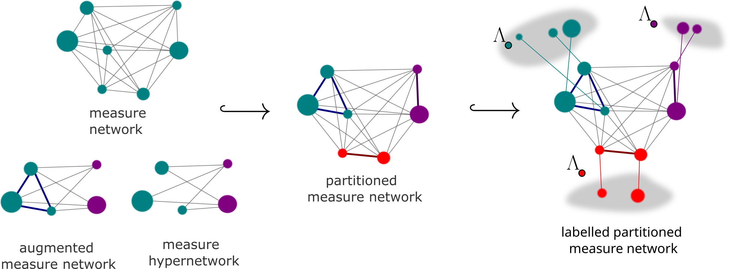
Figure 1: A schematic representation of the types of generalized networks which can be embedded into the space of partitioned measure networks. From left to right: (i) examples of a measure network, augmented measure network and measure hypernetwork. (ii) Illustration of a partitioned measure network with $k=3$ partitions. (iii) Illustration of a labeled partitioned measure network.

Our contributions include:

• We equip the space of partitioned measure networks with a family of transport-based distances $d_{\mathcal{P}_{k}^{p}}$, for $p\geq 1$, formulated as the minimum of a quadratic distortion functional over $k$-partitioned couplings—these are measure couplings which respect the class structures of the partitioned networks. This choice of distance is shown to be a bona fide metric (up to a natural equivalence relation), and we explicitly construct isometric embeddings of measure networks, hypernetworks, and augmented measure networks into this space. See Definition 8 and Theorem 15.

• We furthermore characterize geodesics in the space of partitioned measure networks and show that it is an Alexandrov space with curvature bounded below, see Theorem 21. As an extension to our analysis, we consider addition of labels to partitioned measure networks, which provides a generalization of the so-called fused Gromov-Wasserstein problem [62]. When labels reside in a Hilbert space, we show that our geometric characterization of geodesics and curvature also applies, see Theorem 32.

• Our theoretical contributions provide a unified treatment of a family of generalized networks, which encompass a number of network objects recently introduced in the literature [17, 59, 20, 23]. This allows us to provide a common geometric description of each of these spaces. To our knowledge, in the setting of labeled measure networks, measure hypernetworks, and augmented measure networks, these characterizations are new. We conclude with a brief discussion of the Riemannian geometric concepts of tangent spaces, exponential and logarithmic maps, and gradients in the space of $k$-partitioned measure networks, which will be crucial for practical applications in learning algorithms. We remark here that the recent paper [4] also provides a general framework for studying several variants of the Gromov-Wasserstein distance, but that the results therein are disjoint from the ones presented here: the framework of the present paper captures different variants of Gromov-Wasserstein distance than that of [4], and the curvature bounds and Riemannian structures established here are not treated in [4].

• We illustrate our framework in in-depth computational case studies, which bring together the theoretical ideas that we have introduced. We provide a connection between the Gromov-Wasserstein network matching problem and a family of spectral network alignment algorithms [25, 38]. To our knowledge, this connection has not been explicitly pointed out in the literature previously. We show that partitioned measure networks provide a more natural and flexible extension to the hypergraph alignment problem, and we demonstrate in numerical experiments that transport-based approaches are more accurate and efficient than spectral methods.

• We further illustrate our methods in action in applications to metabolic network alignment, simultaneous sample and feature alignment in multi-omics data, and multi-scale network matching. We formulate each of these problems in terms of partitioned network matching. Last, we take a look at some more involved problems on the space of partitioned networks that exploit its geometric properties. For example, we provide computational characterizations of geodesics and barycenters in the space of measure hypernetworks. We introduce geodesic dictionary learning as a bilevel problem on the space of (partitioned) measure networks, from which we motivate linearized dictionary learning [65] as a fast approximate algorithm. We conclude by demonstrating the utility of this approach in a synthetic hypergraph block model and with partitioned networks derived from atom and topological representations of small molecules.

2 Metric Geometry of Spaces of Generalized Networks

2.1 Spaces of Generalized Networks

We first review some notions of generalized networks, and Gromov-Wasserstein-like distances between them, which have appeared previously in the literature.

2.1.1 Generalized Networks

Let us first recall some definitions of generalized network structures in the literature. These use the following notational conventions: given measure spaces $(X,\mu)$ and $(Y,\nu)$, we use $L^{p}(\mu)$ to denote the space of $p$-integrable functions on $X$ (for $p\in[1,\infty]$) and we use $\mu\otimes\nu$ to denote the product measure on $X\times Y$.

Definition 1 (Generalized Networks).

Let $p\in[1,\infty]$.

1. A measure $p$-network [17] is a triple $N=(X,\mu,\omega)$, where $X$ is a Polish space, $\mu$ is a Borel probability measure on $X$, and $\omega:X\times X\to[0,\infty)$ is an element of $L^{p}(\mu\otimes\mu)$. Let $\mathcal{N}^{p}$ denote the collection of all measure $p$-networks.

2. A measure $p$-hypernetwork [59, 20] is a five-tuple $H=(X,\mu,Y,\nu,\omega)$ consisting of Polish spaces $X$ and $Y$ endowed with Borel probability measures $\mu$ and $\nu$, respectively, and $\omega:X\times Y\to[0,\infty)$ is an element of $L^{p}(\mu\otimes\nu)$. Let $\mathcal{H}^{p}$ denote the collection of all measure $p$-hypernetworks.

3. An augmented measure $p$-network [23] is a six-tuple $A=(X,\mu,Y,\nu,\omega_{X},\omega_{XY})$, consisting of Polish spaces $X$ and $Y$ endowed with Borel probability measures $\mu$ and $\nu$, respectively, and $\omega_{X}:X\times X\to[0,\infty)$ and $\omega_{XY}:X\times Y\to[0,\infty)$ are elements of $L^{p}(\mu\otimes\mu)$ and $L^{p}(\mu\otimes\nu)$, respectively. Let $\mathcal{A}^{p}$ denote the collection of all augmented measure $p$-networks.

We will frequently suppress explicit mention of the parameter $p$, as the appropriate value will typically be either unimportant or clear from context; e.g., when referring to certain $L^{p}$-type metrics. The functions $\omega$, $\omega_{X}$, $\omega_{XY}$, etc., will loosely be referred to as network kernels.

Example 2.

We now provide prototypical examples of the structures defined above.

1. A metric measure space is a measure network $(X,\mu,\omega)$ such that $\omega$ satisfies the axioms of a metric, and the topology of $X$ is induced by the metric. This was the original setting where the Gromov-Wasserstein distances were formulated—see [35, 36], as well as the related work [54]. More general examples of measure networks frequently come from the setting of graph theory, where $X$ is a finite set of vertices, $\omega$ is a graph kernel, and $\mu$ is some choice of weights on the nodes (e.g., uniform). For example, weighted adjacency functions are used as network kernels in this framework to represent protein-protein interaction networks in [68], and heat kernels are used in [19] for the purpose of uncovering community structures in graph datasets.

2. A hypergraph is a set $V$ of vertices and a set $E$ of subsets of $V$, each of which is referred to as a hyperedge. The containment or incidence relation can be encoded as a function $\omega:V\times E\to\{0,1\}$, so that picking probability measures $\mu$ and $\nu$ (say, uniform) yields a measure hypernetwork $(V,\mu,E,\nu,\omega)$. This representation was used in [20], where it was applied, for example, to simplify hypergraphs representing complicated social interactions. The notion of a measure hypernetwork therefore generalizes the notion of a hypergraph. One also obtains a measure hypernetwork from a data matrix, where $X$ is an indexing set for samples, $Y$ is an indexing set for features , $\omega(x,y)$ is the value of the matrix for sample $x$ and feature $y$ and $\mu$ and $\nu$ are some choices of weights. Applications to analysis of ensembles of data matrices was a main motivation for the introduction of this formalism in [59].

3. One can obtain an augmented measure network by taking $(X,\mu,Y,\nu,\omega)$ to be a measure hypernetwork representation of a data matrix, setting $\omega_{XY}=\omega$ and taking $\omega_{X}$ to be some relational function on the rows, such as distance between samples in the data space. This approach was taken to model multi-omics data in [23], with a view toward integrating several single-cell multi-omics datasets.

Remark 3 (Representations as Graph Structures).

Figure 1 provides schematic representations of the generalized networks defined above. To interpret this, one should conceptualize a measure network as a fully connected, weighted graph with node set $X$ and edge weights encoded by $\omega$. From this perspective, it is natural to consider a measure hypernetwork as a bipartite weighted graph, where $X$ and $Y$ define the two classes of nodes. Then $\omega$ defines edge weights for the complete bipartite graph, while there are no edges joining pairs of nodes in $X$ or pairs in $Y$. Finally, an augmented measure network can be viewed similarly, with the difference being that edges between nodes in $X$ are permitted, with weights encoded by $\omega_{X}$ (bipartite edge weights being encoded by $\omega_{XY}$). These interpretations lead to the $k$-partitioned measure network formalism introduced in Section 2.2.

Remark 4 (Finite and Continuous Spaces).

The concept of measure hypernetwork was introduced in [59], somewhat less formally, and primarily as a model for data matrices (so $X$ and $Y$ were assumed to be finite). This definition was formalized and extended to the setting of infinite spaces in [20] (in a slightly less general form than what is presented here, as network kernels were assumed therein to be bounded and the underlying Polish spaces were assumed to be compact for many results). The computational examples of practical interest are, of course, always defined over finite spaces; the main motivation for extending the definition to infinite spaces is to allow us to consider the collection of all measure hypernetworks as a complete metric space with respect to the distance defined below. Similarly, the notion of an augmented measure network was introduced for finite spaces in [23], and the more formal definition provided above is novel.

2.1.2 Generalized Network Distances

For each flavor of generalized network described in Definition 1, there has been an associated notion of distance introduced in the literature. They all have a similar structure, defined in terms of optimizing over measure couplings, as in the Kantorovich formulation of classical optimal transport (see [64, 42] as general references on optimal transport). Below, we use $\mathrm{proj}_{X}:X\times X^{\prime}\to X$ and $\mathrm{proj}_{X^{\prime}}:X\times X^{\prime}\to X^{\prime}$ to denote coordinate projections on product sets, and for a Borel measurable map $p:X\to Y$ of topological spaces, we use $p_{\#}\mu$ to denote the pushforward to $Y$ of a Borel measure $\mu$ on $X$.

Definition 5 (Measure Coupling).

For probability spaces $(X,\mu)$ and $(X^{\prime},\mu^{\prime})$, we say that a measure $\pi$ on $X\times X^{\prime}$ is a coupling of $\mu$ and $\mu^{\prime}$ if its left and right marginals are equal to $\mu$ and $\mu^{\prime}$, respectively—that is, $(\mathrm{proj}_{X})_{\#}\pi=\mu$ and $(\mathrm{proj}_{X^{\prime}})_{\#}\pi=\mu^{\prime}$. Let $\Pi(\mu,\mu^{\prime})$ denote the set of all couplings of $\mu$ and $\mu^{\prime}$.

Let us now establish some convenient notational conventions that will be used throughout the rest of the paper. We always use $N$ and $N^{\prime}$ to stand for measure networks, with the underlying data always being implicitly denoted $N=(X,\mu,\omega)$ and $N^{\prime}=(X^{\prime},\mu^{\prime},\omega^{\prime})$. We similarly use $H,H^{\prime}$ for measure hypernetworks and $A,A^{\prime}$ for augmented hypernetworks. That is, when referring to $H$, the underlying data is implicitly given by $H=(X,\mu,Y,\nu,\omega)$, unless explicitly stated otherwise. For functions $\tau:A\times B\to\mathbb{R}$ and $\tau^{\prime}:A^{\prime}\times B^{\prime}\to\mathbb{R}$, the difference $\tau-\tau^{\prime}$ is understood to be the function defined on $A\times A^{\prime}\times B\times B^{\prime}$ as follows:

$$\tau-\tau^{\prime}:A\times A^{\prime}\times B\times B^{\prime} \to\mathbb{R}$$

$$(a,a^{\prime},b,b^{\prime}) \mapsto\tau(a,b)-\tau^{\prime}(a^{\prime},b^{\prime}).$$

Given a measure space $(X,\mu)$, we use $\|\cdot\|_{L^{p}(\mu)}$ to denote the standard norm on $L^{p}(\mu)$. With these conventions in mind, we recall some metrics which have been introduced on the generalized network spaces of Definition 1.

Definition 6 (Generalized Network Distances).

Let $p\in[1,\infty]$.

1. The network $p$-distance or Gromov-Wasserstein $p$-distance[17] between measure networks $N,N^{\prime}\in\mathcal{N}^{p}$ is

   $$d_{\mathcal{N}^{p}}(N,N^{\prime}):=\inf_{\pi\in\Pi(\mu,\mu^{\prime})}\frac{1}{2}\|\omega-\omega^{\prime}\|_{L^{p}(\pi\otimes\pi)}.$$

2. The hypernetwork $p$-distance [59, 20] between measure hypernetworks $H,H^{\prime}\in\mathcal{H}^{p}$ is

   $$d_{\mathcal{H}^{p}}(H,H^{\prime}):=\inf_{\begin{subarray}{c}\pi\in\Pi(\mu,\mu^{\prime})\\ \xi\in\Pi(\nu,\nu^{\prime})\end{subarray}}\frac{1}{2}\|\omega-\omega^{\prime}\|_{L^{p}(\pi\otimes\xi)}.$$

3. The augmented network $p$-distance [23] between augmented measure networks $A,A^{\prime}\in\mathcal{A}^{p}$ is

   $$d_{\mathcal{A}^{p}}(A,A^{\prime}):=\inf_{\begin{subarray}{c}\pi\in\Pi(\mu,\mu^{\prime})\\ \xi\in\Pi(\nu,\nu^{\prime})\end{subarray}}\frac{1}{2}\left(\|\omega_{X}-\omega_{X^{\prime}}^{\prime}\|_{L^{p}(\pi\otimes\pi)}^{p}+\|\omega_{XY}-\omega_{X^{\prime}Y^{\prime}}^{\prime}\|_{L^{p}(\pi\otimes\xi)}^{p}\right)^{1/p}.$$

In the following subsection, we unify these various generalized network concepts and distances (as well as others) under a common framework. We will use this common framework to derive various metric properties of these distances simultaneously.

2.2 Partitioned Measure Networks and Generalized Networks

One should observe the similarities between the various notions of generalized network in Definition 1, and the optimal transport-inspired distances between them described in Definition 6. In this section, we describe a new structure which simultaneously generalizes these ideas.

2.2.1 Partitioned Measure Networks

Let us now introduce a new generalized network structure.

Definition 7 (Partitioned Measure Network).

Let $k$ be a positive integer and $p\in[1,\infty]$. A $k$-partitioned measure $p$-network is a structure of the form $P=\big{(}(X_{i},\mu_{i})_{i=1}^{k},\omega\big{)}$, where each $X_{i}$ is a Polish space such that $X_{i}\cap X_{j}=\emptyset$ for $i\neq j$, each $\mu_{i}$ is a Borel probability measure on $X_{i}$, and $\omega:X\times X\to[0,\infty)$ is an element of $L^{p}(\mu\otimes\mu)$, where $\mu:=\sum_{i}\mu_{i}$, considered as a measure on $X:=\sqcup_{i}X_{i}$.

To simplify notation, we sometimes write $(X_{i},\mu_{i})$ instead of $(X_{i},\mu_{i})_{i=1}^{k}$, $(X_{i})$ instead of $(X_{i})_{i=1}^{k}$ and $(\mu_{i})$ instead of $(\mu_{i})_{i=1}^{k}$. We use $\mathcal{P}_{k}^{p}$ to denote the collection of all $k$-partitioned measure $p$-networks.

It is often the case that the particular values of $k$ and $p$ are not important, in which case we abuse terminology and refer to the objects defined above as partitioned measure networks. In line with those established above, we follow the notational convention that $P$ and $P^{\prime}$ are implicitly assumed to stand for partitioned measure networks $P=((X_{i},\mu_{i}),\omega)$ and $P^{\prime}=((X^{\prime}_{i},\mu_{i}^{\prime}),\omega^{\prime})$. Observe that a $1$-partitioned measure network is just a measure network; that is, $\mathcal{N}^{p}=\mathcal{P}_{1}^{p}$. Next, we observe that there are maps which include the various notions of generalized networks from Definition 1 into $\mathcal{P}_{2}^{p}$.

Definition 8 (Generalized Network Embeddings).

We have the following families of embeddings.

1. For each $k$, let $\varepsilon_{k,k+1}:\mathcal{P}_{k}^{p}\to\mathcal{P}_{k+1}^{p}$ be the map taking $P\in\mathcal{P}_{k}^{p}$ to

   $$\varepsilon_{k,k+1}(P):=\left((X_{i},\mu_{i})_{i=1}^{k+1},\varepsilon_{k,k+1}(\omega)\right),$$

   where $X_{k+1}$ consists of a single abstract point, $\mu_{k+1}$ is the associated Dirac measure, and the network kernel is defined by

   $$\varepsilon_{k,k+1}(\omega):(\sqcup_{i=1}^{k+1}X_{i})\times(\sqcup_{i=1}^{k+1}X_{i})\to\mathbb{R},\qquad\varepsilon_{k,k+1}(\omega)(u,v)=\left\{\begin{array}[]{rl}\omega(u,v)&(u,v)\in(\sqcup_{i=1}^{k}X_{i})\times(\sqcup_{i=1}^{k}X_{i})\\ 0&\mbox{otherwise.}\end{array}\right.$$

   In particular, $\varepsilon_{1,2}$ gives an embedding $\mathcal{N}^{p}\hookrightarrow\mathcal{P}_{2}^{p}$. For $k<\ell$, we define $\varepsilon_{k,\ell}:\mathcal{P}^{p}_{k}\to\mathcal{P}^{p}_{\ell}$ by

   $$\varepsilon_{k,\ell}:=\varepsilon_{\ell-1,\ell}\circ\cdots\circ\varepsilon_{k,k+1}.$$

2. Let $\varepsilon_{\mathcal{H}}:\mathcal{H}^{p}\to\mathcal{P}^{p}_{2}$ be the map taking $H\in\mathcal{H}^{p}$ to

   $$\varepsilon_{\mathcal{H}}(H):=\left(((X,\mu),(Y,\nu)),\varepsilon_{\mathcal{H}}(\omega)\right),$$

   where

   $$\varepsilon_{\mathcal{H}}(\omega)(u,v):=\left\{\begin{array}[]{rl}\omega(u,v)&u\in X\mbox{ and }v\in Y\\ 0&\mbox{otherwise}.\end{array}\right.$$

3. Let $\varepsilon_{\mathcal{A}}:\mathcal{A}^{p}\to\mathcal{P}_{2}^{p}$ be the map taking $A\in\mathcal{A}^{p}$ to

   $$\varepsilon_{\mathcal{A}}(A):=\left(((X,\mu),(Y,\nu)),\varepsilon_{\mathcal{A}}(\omega_{X},\omega_{XY})\right),$$

   where

   $$\varepsilon_{\mathcal{A}}(\omega_{X},\omega_{XY})(u,v):=\left\{\begin{array}[]{rl}\omega_{X}(u,v)&u,v\in X\\ \omega_{XY}(u,v)&u\in X\mbox{ and }v\in Y\\ 0&\mbox{otherwise}.\end{array}\right.$$

Example 9.

The generalized network embeddings defined above show that measure networks, hypernetworks and augmented hypernetworks can be considered as 2-partitioned networks, so that this structure encompasses those described in Example 2. Another source of examples of $k$-partitioned networks is the notion of a dataset with categorical class structure. That is, consider a (say, finite) dataset of points $X$ such that each $x\in X$ belongs to one of $k$ different classes—for example, $X$ could consist of a set of images, and the images could be assigned classes based on subject matter (e.g., cats, dogs, etc.). This class structure can be encoded as probability measures by taking $\mu_{i}$ to be a uniform measure supported on those points belonging to class $i$. The supports then define the required partition of $X=\sqcup_{i}X_{i}$ and any choice of network kernel $\omega$ on $X$ gives a representation of the multiclass dataset as a $k$-partitioned measure network.

Remark 10 (Intuition for the Embeddings).

Remark 3 gave interpretations of generalized networks in terms of graph structures, illustrated schematically in Figure 1. The embeddings defined above formalize these intuitive descriptions mathematically. For example, if $H\in\mathcal{H}^{p}$ is a representation of a hypergraph, then $\varepsilon_{\mathcal{H}}(H)$ gives a representation of $H$ as a bipartite graph.

2.2.2 Partitioned Network Distance

We now define a distance between partitioned measure networks, using the concept of a partitioned coupling.

Definition 11 (Partitioned Coupling).

Given $k$-tuples of probability spaces $(X_{i},\mu_{i})_{i=1}^{k}$ and $(X^{\prime}_{i},\mu_{i}^{\prime})_{i=1}^{k}$, let

$$\Pi_{k}((\mu_{i}),(\mu_{i}^{\prime})):=\Pi(\mu_{1},\mu_{1}^{\prime})\times\cdots\times\Pi(\mu_{k},\mu_{k}^{\prime}).$$

An element $(\pi_{i})_{i=1}^{k}$ of $\Pi_{k}((\mu_{i}),(\mu_{i}^{\prime}))$ will be referred to as a $k$-partitioned coupling. To simplify notation, we sometimes denote $k$-partitioned couplings as $(\pi_{i})$ instead of $(\pi_{i})_{i=1}^{k}$.

Definition 12 (Partitioned Network Distance).

For $p\in[0,\infty)$, the partitioned network $p$-distance between partitioned measure networks $P,P^{\prime}\in\mathcal{P}_{k}^{p}$ is

$$d_{\mathcal{P}_{k}^{p}}(P,P^{\prime}):=\inf_{(\pi_{i})\in\Pi_{k}((\mu_{i}),(\mu^{\prime}_{i}))}\frac{1}{2}\left(\sum_{i,j=1}^{k}\|\omega-\omega^{\prime}\|_{L^{p}(\pi_{i}\otimes\pi_{j})}^{p}\right)^{1/p}.$$ (1)

For $p=\infty$, we define

$$d_{\mathcal{P}_{k}^{\infty}}(P,P^{\prime}):=\inf_{(\pi_{i})\in\Pi_{k}((\mu_{i}),(\mu_{i}^{\prime}))}\frac{1}{2}\max_{i,j}\|\omega-\omega^{\prime}\|_{L^{\infty}(\pi_{i}\otimes\pi_{j})}.$$ (2)

Remark 13.

In the above definition and throughout the rest of the paper, we slightly abuse terminology and consider each $\pi_{i}$ as a probability measure on $(\sqcup_{j}X_{j})\times(\sqcup_{j}X_{j}^{\prime})$ which is supported on the subset $X_{i}\times X_{i}^{\prime})$.

Remark 14 (Connection to Labeled Gromov-Wasserstein Distance [47]).

A notion of GW distance is introduced which is essentially equivalent to our partitioned network distance [47]. However, the treatment in that paper is very much from a computational perspective, and a formal, general definition of the distance is not provided. The usefulness of such a metric is demonstrated by applications to cross-modality matching for biological data. We remark that [47] uses the terminology labeled Gromov-Wasserstein distance; we use the term labeled differently below, in Section 3.

When $k=1$, $d_{\mathcal{P}_{1}^{p}}$ is simply the Gromov-Wasserstein distance $d_{\mathcal{N}^{p}}$. We will show below that, for arbitrary $k$, $d_{\mathcal{P}_{k}^{p}}$ induces a metric on $\mathcal{P}_{k}^{p}$ modulo a natural notion of equivalence, which generalizes the known result in the Gromov-Wasserstein case. Before doing so, we show that the embeddings of generalized networks of Definition 8 preserve the notions of distance that we have defined so far.

Theorem 15.

The maps from Definition 8 preserve generalized network distances:

1. for $k<\ell$, $d_{\mathcal{P}_{\ell}^{p}}(\varepsilon_{k,\ell}(P),\varepsilon_{k,\ell}(P^{\prime}))=d_{\mathcal{P}_{k}^{p}}(P,P^{\prime})$; in particular, $d_{\mathcal{P}_{2}^{p}}(\varepsilon_{1,2}(N),\varepsilon_{1,2}(N^{\prime}))=d_{\mathcal{N}^{p}}(N,N^{\prime})$,

2. $d_{\mathcal{P}_{2}^{p}}(\varepsilon_{\mathcal{H}}(H),\varepsilon_{\mathcal{H}}(H^{\prime}))=d_{\mathcal{H}^{p}}(H,H^{\prime})$, and

3. $d_{\mathcal{P}_{2}^{p}}(\varepsilon_{\mathcal{A}}(A),\varepsilon_{\mathcal{A}}(A^{\prime}))=d_{\mathcal{A}^{p}}(A,A^{\prime})$.

Proof.

We provide details for the $p<\infty$ case, with the proof for $p=\infty$ following by similar arguments. For the first claim, it suffices to consider the case where $\ell=k+1$. Let $P,P^{\prime}\in\mathcal{P}_{k}^{p}$. Any $(\pi_{i})=(\pi_{i})_{i=1}^{k}\in\Pi_{k}((\mu_{i}),(\mu_{i}^{\prime}))$ extends uniquely to a $(k+1)$-partitioned coupling of $(\mu_{1},\ldots,\mu_{k},\mu_{k+1})$ and $(\mu_{1}^{\prime},\ldots,\mu_{k}^{\prime},\mu_{k+1}^{\prime})$—namely, $(\pi_{1},\ldots,\pi_{k},\pi_{k+1})$, where $\pi_{k+1}$ the Dirac mass on the singleton set $X_{k+1}\times X_{k+1}^{\prime}$. We have that

$$\sum_{i,j=1}^{k+1}\|\varepsilon_{k,k+1}(\omega)-\varepsilon_{k,k+1}(\omega^{\prime})\|_{L^{p}(\pi_{i}\otimes\pi_{j})}^{p} =\sum_{i=1}^{k+1}\|\varepsilon_{k,k+1}(\omega)-\varepsilon_{k,k+1}(\omega^{\prime})\|_{L^{p}(\pi_{i}\otimes\pi_{k+1})}^{p}$$

$$\qquad+\sum_{j=1}^{k+1}\|\varepsilon_{k,k+1}(\omega)-\varepsilon_{k,k+1}(\omega^{\prime})\|_{L^{p}(\pi_{k+1}\otimes\pi_{j})}^{p}$$

$$\qquad\qquad+\sum_{i,j=1}^{k}\|\varepsilon_{k,k+1}(\omega)-\varepsilon_{k,k+1}(\omega^{\prime})\|_{L^{p}(\pi_{i}\otimes\pi_{j})}^{p}$$

$$=\sum_{i,j=1}^{k}\|\omega-\omega^{\prime}\|_{L^{p}(\pi_{i}\otimes\pi_{j})}^{p},$$

where the last line follows because $\varepsilon_{k,k+1}(\omega)=\varepsilon_{k,k+1}(\omega^{\prime})=0$ on the supports of $\pi_{i}\otimes\pi_{k+1}$ and $\pi_{k+1}\otimes\pi_{j}$ and, moreover, $\varepsilon_{k,k+1}(\omega)=\omega$ and $\varepsilon_{k,k+1}(\omega^{\prime})=\omega^{\prime}$ on the support of each $\pi_{i}\otimes\pi_{j}$ with $i,j<k$. Since the $k$-partitioned coupling $(\pi_{i})$ was arbitrary, the first claim follows.

Let us now prove the third claim; the case for hypernetworks is proved using similar arguments, so we omit the details here. Let $A,A^{\prime}\in\mathcal{A}^{p}$ and let $\pi\in\Pi(\mu,\mu^{\prime})$ and $\xi\in\Pi(\nu,\nu^{\prime})$. Then $(\pi_{1},\pi_{2})=(\pi,\xi)$ is a $2$-partitioned coupling of $(\mu,\nu)$ and $(\mu^{\prime},\nu^{\prime})$, and we have

$$\sum_{i,j=1}^{2}\|\varepsilon_{\mathcal{A}}(\omega)-\varepsilon_{\mathcal{A}}(\omega^{\prime})\|_{L^{p}(\pi_{i}\otimes\pi_{j})}^{p}=\|\omega_{X}-\omega_{X^{\prime}}^{\prime}\|_{L^{p}(\pi\otimes\pi)}^{p}+\|\omega_{XY}-\omega_{X^{\prime}Y^{\prime}}^{\prime}\|_{L^{p}(\pi\otimes\xi)}^{p},$$

by reasoning similar to the above. Since $\pi$ and $\xi$ were arbitrary, this completes the proof.

∎

2.2.3 Metric Properties of Partitioned Network Distance

To describe the exact sense in which $d_{\mathcal{P}_{k}^{p}}$ is a distance, we need to introduce some equivalence relations on partitioned measure networks.

Definition 16 (Strong and Weak Isomorphism).

We say that $k$-partitioned measure networks $P$ and $P^{\prime}$ are strongly isomorphic if, for each $i=1,\ldots,k$, there is a Borel measurable bijection $\phi_{i}:X_{i}\to X^{\prime}_{i}$ (with Borel measurable inverse) such that $(\phi_{i})_{\#}\mu_{i}=\mu_{i}^{\prime}$, and $\omega(x,y)=\omega^{\prime}(\phi_{i}(x),\phi_{j}(y))$ for every pair $(x,y)\in X_{i}\times X_{j}$. The tuple $(\phi_{i})$ is called a strong isomorphism.

A tuple $(\phi_{i})$ of maps $\phi_{i}:X_{i}\to X_{i}^{\prime}$ is called a weak isomorphism from $P$ to $P^{\prime}$ if $(\phi_{i})_{\#}\mu_{i}=\mu_{i}^{\prime}$, and $\omega(x,y)=\omega^{\prime}(\phi_{i}(x),\phi_{j}(y))$ for $\mu_{i}\otimes\mu_{j}$-almost every pair $(x,y)\in X_{i}\times X_{j}$.

We say that $P$ and $P^{\prime}$ are weakly isomorphic if there exists a third partitioned measure network $\overline{P}=((\overline{X}_{i},\overline{\mu}_{i}),\overline{\omega})$ and weak isomorphisms $(\phi_{i})$ from $\overline{P}$ to $P$ and $(\phi_{i}^{\prime})$ from $\overline{P}$ to $P^{\prime}$.

It is straightforward to show that weak isomorphism defines an equivalence relation on $\mathcal{P}$; we use $P\sim P^{\prime}$ to denote that $P$ is weakly isomorphic to $P^{\prime}$. For $P\in\mathcal{P}_{k}^{p}$, let $[P]$ denote its equivalence class under this relation and let $[\mathcal{P}_{k}^{p}]$ denote the collection of all equivalence classes.

Using the embeddings from Definition 8, there is an induced notion of weak isomorphism on the spaces of generalized networks. Let $[\mathcal{N}^{p}]$, $[\mathcal{H}^{p}]$ and $[\mathcal{A}^{p}]$ denote the collections of weak isomorphism equivalence classes of measure networks, measure hypernetworks and augmented measure networks, respectively.

Weak isomorphisms of measure networks and of measure hypernetworks are introduced in [17] and [20], respectively. It is straightforward to show that the induced notions from Definition 16 agree with those already established in the literature. These papers show that $d_{\mathcal{N}^{p}}$ and $d_{\mathcal{H}^{p}}$ descend to well-defined metrics on $[\mathcal{N}^{p}]$ and $[\mathcal{H}^{p}]$, respectively. The following theorem generalizes these results, in light of Theorem 15.

Theorem 17.

The $k$-partitioned network $p$-distance $d_{\mathcal{P}_{k}^{p}}$ induces a well-defined metric on $[\mathcal{P}_{k}^{p}]$.

Putting Theorems 15 and 17 together, we obtain the following corollary.

Corollary 18.

The generalized network distances $d_{\mathcal{N}^{p}}$, $d_{\mathcal{H}^{p}}$ and $d_{\mathcal{A}^{p}}$ induce well-defined metrics on $[\mathcal{N}^{p}]$, $[\mathcal{H}^{p}]$ and $[\mathcal{A}^{p}]$, respectively. The embeddings from Definition 8 induce isometric embeddings of each of these spaces into $[\mathcal{P}_{2}^{p}]$.

We will abuse notation and continue to denote the induced metric on $[\mathcal{P}_{k}^{p}]$ as $d_{\mathcal{P}_{k}^{p}}$, and take a similar convention for the other induced metrics.

Remark 19.

The case of $\mathcal{N}^{p}$ in the corollary was proved in [17] and the case of $\mathcal{H}^{p}$ was proved in [20] (those papers assumed boundedness of the $\omega$-functions, but this restriction is easily lifted in those proofs). In [23], a relaxed version of triangle inequality was proved for the augmented network distance in the finite setting. Our result is a strengthening of this.

Theorem 17 follows as an easy corollary of a more general result in the following section, so we defer its proof to Section 3.1.2.

2.2.4 Geodesics and Curvature

We can say more about the metric properties of the partitioned network distance. To state our next result, we first recall some standard concepts from metric geometry; see [7, 10] as general references.

Definition 20 (Geodesics and Curvature).

Let $(X,d)$ be a metric space.

1. A geodesic between points $x,y\in X$ is a path $\gamma:[0,1]\to X$ with $\gamma(0)=x$, $\gamma(1)=y$ and such that, for all $0\leq s\leq t\leq 1$, we have

   $$d(\gamma(s),\gamma(t))=(t-s)d(x,y).$$

   If there is a geodesic joining any two points in $X$, we say that $(X,d)$ is a geodesic space.

2. Suppose that $(X,d)$ is a geodesic space. We say that $(X,d)$ has curvature bounded below by zero if for every geodesic $\gamma:[0,1]\to X$ and every point $x\in X$, we have

   $$d(\gamma(t),x)^{2}\geq(1-t)d(\gamma(0),x)^{2}+td(\gamma(1),x)^{2}-t(1-t)d(\gamma(0),\gamma(1))^{2}$$

   for all $t\in[0,1]$.

3. We say that $(X,d)$ is an Alexandrov space of non-negative curvature if it is a complete geodesic space with curvature bounded below by zero.

The next main result also follows from a more general result below. We return to the proof of the next result in Section 3.2.3.

Theorem 21.

For any $k\geq 1$, $([\mathcal{P}_{k}^{2}],d_{\mathcal{P}_{k}^{2}})$ is an Alexandrov space of non-negative curvature.

Combining Theorem 21 with Corollary 18 immediately yields the following result.

Corollary 22.

Each of the spaces $([\mathcal{N}^{2}],d_{\mathcal{N}^{2}})$, $([\mathcal{H}^{2}],d_{\mathcal{H}^{2}})$ and $([\mathcal{A}^{2}],d_{\mathcal{A}^{2}})$ is an Alexandrov space of non-negative curvature.

Remark 23.

The fact that $([\mathcal{N}^{2}],d_{\mathcal{N}^{2}})$ is an Alexandrov space of non-negative curvature was essentially proved by Sturm in [55, Theorem 5.8] (there the space of symmetric measure networks was considered, i.e., where the function $\omega:X\times X\to\mathbb{R}$ is assumed to be symmetric; the proof still works if this assumption is dropped, as was observed in [18]). This result is new for the other spaces of generalized networks.

3 Extension to Labeled Networks

We consider, as an extension to the discussion so far, the setting of $k$-partitioned measure networks where each element of the $X_{i},1\leq i\leq k$, is associated with a label element that lives in a metric space.

3.1 Labeled partitioned measure networks

Let us begin by defining a labeled notion of a $k$-partitioned measure network, and the distances between these objects.

Definition 24 (Labeled $k$-partitioned measure networks).

Let $(\Lambda_{i},d_{\Lambda_{i}})$, $1\leq i\leq k$, be fixed metric spaces, which we consider as spaces of labels. A labeled $k$-partitioned measure $p$-network is a tuple $(P,(\iota_{i})_{i=1}^{k})$, where $P=\big{(}(X_{i},\mu_{i})_{i=1}^{k},\omega\big{)}\in\mathcal{P}_{k}^{p}$ and each of the $\iota_{i}:X_{i}\to\Lambda_{i}$ is a measurable function, which we refer to as a labeling function. Further, we assume that each function $X_{i}\times X_{i}\to\mathbb{R}$ defined by $(x,y)\mapsto d_{\Lambda_{i}}(\iota_{i}(x),\iota_{i}(y))$ belongs to $L^{p}(\mu_{i}\otimes\mu_{i})$.

We frequently simplify notation and write $L=(P,(\iota_{i}))$ for a labeled $k$-partitioned network. We denote by $\operatorname{\mathcal{L}\mathcal{P}}_{k}^{p}$ the space of labeled $k$-partitioned measure $p$-networks, where it is understood that the label spaces $(\Lambda_{i},d_{\Lambda_{i}})$ are fixed.

The partitioned network distance (12) can be naturally generalized to $\operatorname{\mathcal{L}\mathcal{P}}_{k}^{p}$.

Definition 25 (Labeled Partitioned Network Distance).

Let $1\leq p<\infty$ and let $L=(P,(\iota_{i})),L^{\prime}=(P^{\prime},(\iota^{\prime}_{i}))\in\operatorname{\mathcal{L}\mathcal{P}}_{k}^{p}$ be two labeled partitioned measure networks. Then we define the labeled $k$-partitioned network distance to be

$$d_{\operatorname{\mathcal{L}\mathcal{P}}_{k}^{p}}(L,L^{\prime})=\inf_{(\pi_{i})\in\Pi_{k}((\mu_{i}),(\mu_{i}^{\prime}))}\frac{1}{2}\left(\sum_{i,j=1}^{k}\|\omega-\omega^{\prime}\|_{L^{p}(\pi_{i}\otimes\pi_{j})}^{p}+\sum_{i=1}^{k}\|d_{\Lambda_{i}}\circ(\iota_{i},\iota^{\prime}_{i})\|_{L^{p}(\pi_{i})}^{p}\right)^{1/p}.$$ (3)

This extends to the $p=\infty$ case as

$$d_{\operatorname{\mathcal{L}\mathcal{P}}_{k}^{\infty}}(L,L^{\prime})=\inf_{(\pi_{i})\in\Pi_{k}((\mu_{i}),(\mu_{i}^{\prime}))}\frac{1}{2}\max\left(\max_{i,j}\|\omega-\omega^{\prime}\|_{L^{\infty}(\pi_{i}\otimes\pi_{j})},\max_{i}\|d_{\Lambda_{i}}\circ(\iota_{i},\iota^{\prime}_{i})\|_{L^{\infty}(\pi_{i})}\right).$$ (4)

Remark 26.

One could include a balance parameter to weight the contributions of the network kernel term (i.e., the first summation) versus the labeling function term (the second summation) in this definition. Such a parameter is included in the definition of Fused Gromov-Wasserstein (FGW) distance [62], which has a similar structure. The connection between $d_{\operatorname{\mathcal{L}\mathcal{P}}_{k}^{p}}$ and FGW distance is explained precisely in Section 3.1.2. We avoid the inclusion of the balance parameter in our formulation, as it is unimportant from a theoretical standpoint and can been absorbed into the definitions of network kernels and label functions in practical applications.

Example 27.

The main examples of labeled partitioned networks come from node-attributed network structures. For example, consider a measure network $N=(X,\mu,\omega)\in\mathcal{N}^{p}$ representing a graph via some graph kernel $\omega$. In applications, the node set $X$ may be attributed with auxiliary data—for example, if the graph encodes user interactions on a social network, then each node may be attributed with additional user-level statistics. This situation can be modeled as a function $\iota:X\to\Lambda$, where $\Lambda$ is the attribute space (e.g., $\Lambda=\mathbb{R}^{n}$). The structure $(N,\iota)$ defines an element of $\operatorname{\mathcal{L}\mathcal{P}}_{1}^{p}$.

A simple (but useful) observation is that the distances can be written as nested $\ell^{p}$-norms. For the rest of the paper, let $\|\cdot\|_{p}$ denote the $\ell^{p}$ norm on $\mathbb{R}^{n}$ for $p\in[1,\infty]$. We abuse notation and use the same symbol $\|\cdot\|_{p}$ for the norm on spaces of various dimensions, with the specific meaning always being clear from context. Then the labeled $k$-partitioned network distance can be expressed as

$$d_{\operatorname{\mathcal{L}\mathcal{P}}_{k}^{p}}(L,L^{\prime})=\inf_{(\pi_{i})\in\Pi_{k}((\mu_{i}),(\mu_{i}^{\prime}))}\frac{1}{2}\left\|\left(\left\|\left(\|\omega-\omega^{\prime}\|_{L^{p}(\pi_{i}\otimes\pi_{j})}\right)_{i,j}\right\|_{p},\left\|\left(\|d_{\Lambda_{i}}\circ(\iota_{i},\iota_{i}^{\prime})\|_{L^{p}(\pi_{i})}\right)_{i}\right\|_{p}\right)\right\|_{p}$$ (5)

for all $p\in[1,\infty]$. We have made one more abuse of notation by considering the collection $\left(\|\omega-\omega^{\prime}\|_{L^{p}(\pi_{i}\otimes\pi_{j})}\right)_{i,j}$, which is most naturally indexed as a $k\times k$ matrix, as an element of $\mathbb{R}^{k^{2}}$ in order to apply the $\ell^{p}$ norm to it.

3.1.1 Metric Properties of the Labeled Distance

We now show that $d_{\operatorname{\mathcal{L}\mathcal{P}}_{k}^{p}}$ defines a metric, up to a natural notion of equivalence. Strong and weak isomorphisms of partitioned networks (Definition 16) extend to the case of labeled partitioned measure networks in a straightforward way.

Definition 28 (Weak Isomorphism of Labeled Partitioned Measure Networks).

We say that labeled $k$-partitioned measure networks $L=(P,(\iota_{i}))$ and $L^{\prime}=(P^{\prime},(\iota_{i}^{\prime}))$ are strongly isomorphic if the underlying partitioned measure networks $P$ and $P^{\prime}$ are strongly isomorphic (see Definition 16) via bijections $\phi_{i}:X_{i}\to X_{i}^{\prime}$ such that $\iota_{i}(x)=\iota^{\prime}_{i}(\phi(x))$ for $\mu_{i}$-almost every $x\in X_{i}$.

We say that $L$ and $L^{\prime}$ are weakly isomorphic if there exists $\overline{L}=(\overline{P},(\overline{\iota}_{i}))\in\operatorname{\mathcal{L}\mathcal{P}}_{k}$, with $\overline{P}=((\overline{X}_{i},\overline{\mu}_{i}),\overline{\omega})$, and bijective maps $\phi_{i}:\overline{X}_{i}\to X_{i}$ and $\phi_{i}^{\prime}:\overline{X}_{i}\to X_{i}^{\prime}$ which make the underlying measure networks weakly isomorphic (see Definition 16) and such that

$$\overline{\iota}_{i}(x)=\iota_{i}(\phi(x))=\iota^{\prime}_{i}(\phi^{\prime}(x))$$

for $\overline{\mu}_{i}$-almost every $x\in\overline{X}_{i}$.

One can easily verify that weak isomorphism again defines an equivalence relation on $\operatorname{\mathcal{L}\mathcal{P}}_{k}^{p}$, and we write $[P,(\iota_{i})]$ for equivalence classes and $[\operatorname{\mathcal{L}\mathcal{P}}_{k}^{p}]$ for the quotient space.

The next theorem establishes some metric properties of $d_{\operatorname{\mathcal{L}\mathcal{P}}_{k}^{p}}$, analogous to Theorem 17.

Theorem 29.

The labeled $k$-partitioned network $p$-distance $d_{\operatorname{\mathcal{L}\mathcal{P}}_{k}^{p}}$ induces a well-defined metric on $[\operatorname{\mathcal{L}\mathcal{P}}_{k}^{p}]$.

The proof will use some important technical lemmas.

Lemma 30.

The infima in (3) and (4) are always realized by partitioned couplings.

Proof.

Let $(P,(\iota_{i})),(P^{\prime},(\iota^{\prime}_{i}))\in\operatorname{\mathcal{L}\mathcal{P}}_{k}^{p}$. We have $\Pi_{k}((\mu_{i}),(\mu^{\prime}_{i}))=\Pi(\mu_{1},\mu_{1}^{\prime})\times\cdots\times\Pi(\mu_{k},\mu_{k}^{\prime})$. By [55, Lemma 1.2], each $\Pi(\mu_{i},\mu_{i}^{\prime})$ is compact (as a subspace of the space of probability measures on $X_{i}\times X_{i}^{\prime}$, with the weak topology), so it follows that $\Pi_{k}((\mu_{i}),(\mu_{i}^{\prime}))$ is compact as well. By the proof of [20, Lemma 24], for each $(i,j)$, the function

$$\Pi(\mu_{i},\mu^{\prime}_{i})\times\Pi(\mu_{j},\mu^{\prime}_{j})\to\mathbb{R}:(\pi_{i},\pi_{j})\mapsto\|\omega-\omega^{\prime}\|_{L^{p}(\pi_{i}\otimes\pi_{j})}$$

is continuous in the $p<\infty$ case and lower semicontinuous in the $p=\infty$ case. Similarly, the function $\Pi(\mu_{i},\mu_{i}^{\prime})\to\mathbb{R}:\pi_{i}\mapsto\|d_{\Lambda_{i}}\circ(\iota_{i},\iota_{i}^{\prime})\|_{L^{p}(\pi_{i})}$ is continuous (respectively, lower semicontinuous) if $p<\infty$ (respectively, $p=\infty$). It is then straightforward to see that the objectives of (3) and (4) inherit these properties as functions on $\Pi_{k}((\mu_{i}),(\mu_{i}^{\prime}))$. In either case, it follows from compactness that the infima are achieved. ∎

The proofs of Theorem 29 and results later in the paper will use the following standard result from optimal transport theory. In the statement, and throughout the paper, we use $\mathrm{proj}_{i}:Y^{0}\times Y^{1}\times\cdots\times Y^{n}\rightarrow Y^{i}$ to denote the coordinate projection map from a product of sets to its $i$th factor.

Lemma 31 (Gluing Lemma; see, e.g., Lemma 1.4 of [55]).

Let $(Y_{i},\nu_{i})$, $i=0,\ldots,n$, be Polish probability spaces. For a collection of measure couplings $\xi_{i}\in\Pi(\nu_{i-1},\nu_{i})$, $i=1,\ldots,n$, there is a unique probability measure $\tilde{\xi}$ on $Y_{0}\times Y_{1}\times\cdots\times Y_{n}$ with the property that

$$\big{(}\mathrm{proj}_{i-1}\times\mathrm{proj}_{i}\big{)}_{\#}\tilde{\xi}=\xi_{i}$$

for all $i=1,\ldots,n$.

The measure $\tilde{\xi}$ from the lemma is called the gluing of the measures $\xi_{i}$. We denote it as $\tilde{\xi}=\xi_{1}\boxtimes\xi_{2}\boxtimes\cdots\boxtimes\xi_{n}$.

Proof of Theorem 17.

The function $d_{\operatorname{\mathcal{L}\mathcal{P}}_{k}^{p}}$ is clearly symmetric. We now establish the triangle inequality. Let $L=(P,(\iota_{i})),L^{\prime}=(P^{\prime},(\iota^{\prime}_{i})),L^{\prime\prime}=(P^{\prime\prime},(\iota^{\prime\prime}_{i}))\in\operatorname{\mathcal{L}\mathcal{P}}_{k}^{p}$. By Lemma 30 there exist partitioned couplings $(\pi_{i})\in\Pi_{k}((\mu_{i}),(\mu^{\prime}_{i}))$ and $(\pi_{i}^{\prime})\in\Pi_{k}((\mu^{\prime}_{i}),(\mu^{\prime\prime}_{i}))$ that realize the infima in the distances, respectively, between $P,P^{\prime}$ and $P^{\prime},P^{\prime\prime}$. Let $\widetilde{\xi}_{i}=\pi_{i}\boxtimes\pi_{i}^{\prime}$ denote the probability measure on $X_{i}\times X_{i}^{\prime}\times X_{i}^{\prime\prime}$, for $i=1,\ldots,k$, obtained from the Gluing Lemma. Letting $\xi_{i}$ denote the pushforward to $\widetilde{\xi}_{i}$ to $X_{i}\times X^{\prime\prime}_{i}$, we have that $(\xi_{i})\in\Pi_{k}((\mu_{i}),(\mu_{i}^{\prime\prime}))$. Using the expression (5), we get the desired triangle inequality from the triangle inequality for the $L^{p}$ and $\ell^{p}$-norms and for $d_{\Lambda_{i}}$:

$$2\cdot d_{\operatorname{\mathcal{L}\mathcal{P}}_{k}^{p}}(L,L^{\prime\prime})$$

$$\leq\left\|\left(\left\|\left(\|\omega-\omega^{\prime\prime}\|_{L^{p}(\xi_{i}\otimes\xi_{j})}\right)_{i,j}\right\|_{p},\left\|\left(\|d_{\Lambda_{i}}\circ(\iota_{i},\iota_{i}^{\prime\prime})\|_{L^{p}(\xi_{i})}\right)_{i}\right\|_{p}\right)\right\|_{p}$$

$$=\left\|\left(\left\|\left(\|\omega-\omega^{\prime\prime}\|_{L^{p}(\tilde{\xi}_{i}\otimes\tilde{\xi}_{j})}\right)_{i,j}\right\|_{p},\left\|\left(\|d_{\Lambda_{i}}\circ(\iota_{i},\iota_{i}^{\prime\prime})\|_{L^{p}(\tilde{\xi}_{i})}\right)_{i}\right\|_{p}\right)\right\|_{p}$$

$$\leq\left\|\left(\left\|\left(\|\omega-\omega^{\prime}+\omega^{\prime}-\omega^{\prime\prime}\|_{L^{p}(\tilde{\xi}_{i}\otimes\tilde{\xi}_{j})}\right)_{i,j}\right\|_{p},\left\|\left(\|d_{\Lambda_{i}}\circ(\iota_{i},\iota^{\prime}_{i})+d_{\Lambda_{i}}\circ(\iota^{\prime}_{i},\iota_{i}^{\prime\prime})\|_{L^{p}(\tilde{\xi}_{i})}\right)_{i}\right\|_{p}\right)\right\|_{p}$$

$$\leq\left\|\left(\left\|\left(\|\omega-\omega^{\prime}\|_{L^{p}(\tilde{\xi}_{i}\otimes\tilde{\xi}_{j})}+\|\omega^{\prime}-\omega^{\prime\prime}\|_{L^{p}(\tilde{\xi}_{i}\otimes\tilde{\xi}_{j})}\right)_{i,j}\right\|_{p},\left\|\left(\|d_{\Lambda_{i}}\circ(\iota_{i},\iota^{\prime}_{i})\|_{L^{p}(\tilde{\xi}_{i})}+\|d_{\Lambda_{i}}\circ(\iota^{\prime}_{i},\iota_{i}^{\prime\prime})\|_{L^{p}(\tilde{\xi}_{i})}\right)_{i}\right\|_{p}\right)\right\|_{p}$$

$$\leq\left\|\left(\left\|\left(\|\omega-\omega^{\prime}\|_{L^{p}(\tilde{\xi}_{i}\otimes\tilde{\xi}_{j})}\right)_{i,j}\right\|_{p}+\left\|\left(\|\omega^{\prime}-\omega^{\prime\prime}\|_{L^{p}(\tilde{\xi}_{i}\otimes\tilde{\xi}_{j})}\right)_{i,j}\right\|_{p},\right.\right.$$

$$\hskip 144.54pt\left.\left.\left\|\left(\|d_{\Lambda_{i}}\circ(\iota_{i},\iota^{\prime}_{i})\|_{L^{p}(\tilde{\xi}_{i})}\right)_{i}\right\|_{p}\left\|+\left(\|d_{\Lambda_{i}}\circ(\iota^{\prime}_{i},\iota_{i}^{\prime\prime})\|_{L^{p}(\tilde{\xi}_{i})}\right)_{i}\right\|_{p}\right)\right\|_{p}$$

$$\leq\left\|\left(\left\|\left(\|\omega-\omega^{\prime}\|_{L^{p}(\tilde{\xi}_{i}\otimes\tilde{\xi}_{j})}\right)_{i,j}\right\|_{p},\left\|\left(\|d_{\Lambda_{i}}\circ(\iota_{i},\iota_{i}^{\prime})\|_{L^{p}(\tilde{\xi}_{i})}\right)_{i}\right\|_{p}\right)\right\|_{p}$$

$$\hskip 144.54pt+\left\|\left(\left\|\left(\|\omega^{\prime}-\omega^{\prime\prime}\|_{L^{p}(\tilde{\xi}_{i}\otimes\tilde{\xi}_{j})}\right)_{i,j}\right\|_{p},\left\|\left(\|d_{\Lambda_{i}}\circ(\iota_{i}^{\prime},\iota_{i}^{\prime\prime})\|_{L^{p}(\tilde{\xi}_{i})}\right)_{i}\right\|_{p}\right)\right\|_{p}$$

$$=\left\|\left(\left\|\left(\|\omega-\omega^{\prime}\|_{L^{p}(\tilde{\pi}_{i}\otimes\tilde{\pi}_{j})}\right)_{i,j}\right\|_{p},\left\|\left(\|d_{\Lambda_{i}}\circ(\iota_{i},\iota_{i}^{\prime})\|_{L^{p}(\tilde{\pi}_{i})}\right)_{i}\right\|_{p}\right)\right\|_{p}$$

$$\hskip 144.54pt+\left\|\left(\left\|\left(\|\omega^{\prime}-\omega^{\prime\prime}\|_{L^{p}(\tilde{\pi^{\prime}}_{i}\otimes\tilde{\pi^{\prime}}_{j})}\right)_{i,j}\right\|_{p},\left\|\left(\|d_{\Lambda_{i}}\circ(\iota_{i}^{\prime},\iota_{i}^{\prime\prime})\|_{L^{p}(\tilde{\pi^{\prime}}_{i})}\right)_{i}\right\|_{p}\right)\right\|_{p}$$

$$=2\cdot d_{\operatorname{\mathcal{L}\mathcal{P}}_{k}^{p}}(L,L^{\prime})+2\cdot d_{\operatorname{\mathcal{L}\mathcal{P}}_{k}^{p}}(L^{\prime},L^{\prime\prime}).$$

We note that lines where measures are changed in the $L^{p}$ norms follow by marginalization (for example, the first equality which exchanges $\xi_{i}$ for $\tilde{\xi}_{i}$ and $\xi_{j}$ for $\tilde{\xi}_{j}$). This proves that the triangle inequality holds.

Finally, let us show that $d_{\operatorname{\mathcal{L}\mathcal{P}}_{k}^{p}}(L,L^{\prime})=0$ if and only if $L$ and $L^{\prime}$ are weakly isomorphic. Suppose that $L$ and $L^{\prime}$ are weakly isomorphic. Let $\overline{L}\in\operatorname{\mathcal{L}\mathcal{P}}_{k}$ denote the auxiliary space from the definition of weak isomorphism. It is easy to show that $d_{\operatorname{\mathcal{L}\mathcal{P}}_{k}^{p}}(\overline{L},L)=d_{\operatorname{\mathcal{L}\mathcal{P}}_{k}^{p}}(\overline{L},L^{\prime})=0$, so $d_{\operatorname{\mathcal{L}\mathcal{P}}_{k}^{p}}(L,L^{\prime})=0$ follows by symmetry and the triangle inequality. Conversely, suppose that $d_{\operatorname{\mathcal{L}\mathcal{P}}_{k}^{p}}(L,L^{\prime})=0$. By Lemma 30, there is a partitioned coupling $(\pi_{i})$ such that $\|\omega-\omega^{\prime}\|_{L^{p}(\pi_{i}\otimes\pi_{j})}=\|d_{\Lambda_{i}}\circ(\iota_{i},\iota_{i}^{\prime})\|_{L^{p}(\pi_{i})}=0$ for all $i,j=1,\ldots,k$. Define $\overline{X}_{i}=X_{i}\times X^{\prime}_{i}$, $\overline{\mu}_{i}=\pi_{i}$ and $\overline{\omega}((x,x^{\prime}),(y,y^{\prime}))=\omega(x,y)$. The maps $\phi_{i}:\overline{X}_{i}\to X_{i}$ and $\phi^{\prime}_{i}:\overline{X}_{i}\to X^{\prime}_{i}$ from the definition of weak isomorphism are coordinate projection maps. One can then show that this gives a weak isomorphism of $P$ and $P^{\prime}$. Finally, define a new labeling function $\overline{\iota}_{i}:\overline{X}_{i}\to\Lambda_{i}$ by $\overline{\iota}_{i}(x,x^{\prime})=\iota_{i}(x)$. Since $d_{\Lambda_{i}}$ is a metric, it must be that $\iota_{i}(x)=\iota_{i}^{\prime}(x^{\prime})$ for $\pi_{i}$-almost every $(x,x^{\prime})\in X_{i}\times X_{i}^{\prime}$, so this labeling function satisfies the condition in the definition of weak isomorphism. ∎

3.1.2 Consequences and Comparisons to Other Results

We now give a proof of Theorem 17, which says that the (unlabeled) partitioned network distance is a metric, and which then implies that various other generalized network distances in the literature are metrics as well (Corollary 18).

Proof of Theorem 17.

Consider the map which takes a $k$-partitioned measure network $P$ to the labeled $k$-partitioned measure network $(P,(\iota_{i}))$, where $(\Lambda_{i},d_{\Lambda_{i}})$ is the one-point metric space for all $i$ (hence $\iota_{i}$ is the constant map for all $i$). Clearly, we have

$$d_{\mathcal{P}_{k}^{p}}(P,P^{\prime})=d_{\operatorname{\mathcal{L}\mathcal{P}}_{k}^{p}}\big{(}(P,(\iota_{i})),(P^{\prime},(\iota^{\prime}_{i}))\big{)},$$

since the labeling term in the definition of $d_{\operatorname{\mathcal{L}\mathcal{P}}_{k}^{p}}$ vanishes. Thus the map $P\mapsto(P,(\iota_{i}))$ induces a bijection from $[\mathcal{P}_{k}^{p}]$ to $[\operatorname{\mathcal{L}\mathcal{P}}_{k}^{p}]$ which takes $d_{\mathcal{P}_{k}^{p}}$ to $d_{\operatorname{\mathcal{L}\mathcal{P}}_{k}^{p}}$, and it follows that $d_{\mathcal{P}_{k}^{p}}$ is a metric. ∎

Next, we give a more precise comparison between the distance $d_{\operatorname{\mathcal{L}\mathcal{P}}_{k}^{p}}$ and the Fused Gromov-Wasserstein (FGW) distance of Vayer et al. [62]. The FGW distance is defined in the context of labeled measure networks; that is, in the $k=1$ setting, where we write elements as $(N,\iota)$, with $N=(X,\mu,\omega)\in\mathcal{N}$ and $\iota:X\to\Lambda$, and in which case the distance $d_{\operatorname{\mathcal{L}\mathcal{P}}_{1}^{p}}$ reduces to

$$d_{\operatorname{\mathcal{L}\mathcal{P}}_{1}^{p}}((N,\iota),(N^{\prime},\iota^{\prime}))=\inf_{\pi\in\Pi(\mu,\mu^{\prime})}\frac{1}{2}\left(\|\omega-\omega^{\prime}\|_{L^{p}(\pi\otimes\pi)}^{p}+\|d_{\Lambda}\circ(\iota,\iota^{\prime})\|_{L^{p}(\pi)}^{p}\right)^{1/p},$$ (6)

for $p<\infty$. In contrast, the FGW distance depends on several more parameters, but the version of it which is closest to (6) would read as

$$d_{\mathrm{FGW},p}((N,\iota),(N^{\prime},\iota^{\prime}))$$

$$\qquad\qquad=\inf_{\pi\in\Pi(\mu,\mu^{\prime})}\frac{1}{2}\left(\int_{X\times X^{\prime}\times X\times X^{\prime}}\left(|\omega(x,y)-\omega^{\prime}(x^{\prime},y^{\prime})|+d_{\Lambda}(\iota(x),\iota^{\prime}(x^{\prime}))\right)^{p}d\pi(x,x^{\prime})d\pi(y,y^{\prime})\right)^{1/p}$$

$$\qquad\qquad=\inf_{\pi\in\Pi(\mu,\mu^{\prime})}\frac{1}{2}\||\omega-\omega^{\prime}|+d_{\Lambda}\circ(\iota,\iota^{\prime})\|_{L^{p}(\pi\otimes\pi)}.$$

Although the distances $d_{\operatorname{\mathcal{L}\mathcal{P}}_{1}^{p}}$ and $d_{\mathrm{FGW},p}$ treat the same type of object, the above shows that their formulations are subtly but legitimately distinct.

The situation described above is slightly murky, as several articles following [62] have formulated the FGW distance more in line with (6)–see, e.g., [58, 8, 26]. However, as far as we are aware, the triangle inequality has not previously been established for any version of FGW distance—[62, 58] both give relaxed variants of the triangle inequality for different versions of FGW, where the larger side of the inequality involves an extra scale factor. Theorem 29 therefore gives the first proof of the triangle inequality for FGW, when expressed in the form (6).

3.2 Alexandrov Geometry of Labeled Partitioned Networks

Next, we characterize geodesics and curvature in the space of labeled partitioned measure networks. For the rest of the section, we will assume the following conventions:

• we assume that the label spaces $(\Lambda_{i},d_{\Lambda_{i}})$ are geodesic spaces,

• we will restrict our attention to the case $p=2$, and simply write $\operatorname{\mathcal{L}\mathcal{P}}_{k}$ in place of $\operatorname{\mathcal{L}\mathcal{P}}_{k}^{2}$.

The following is a generalization of Theorem 21; recall that the proof of that theorem was deferred—we will prove it in Section 3.2.3 as a corollary of our next result.

Theorem 32.

Let $\Lambda_{i},1\leq i\leq k$ be a Hilbert space with inner product $\langle\cdot,\cdot\rangle_{\Lambda_{i}}$. Then, for any $k\geq 1$, $([\operatorname{\mathcal{L}\mathcal{P}}_{k}],d_{\operatorname{\mathcal{L}\mathcal{P}}_{k}})$ is an Alexandrov space of non-negative curvature.

We will prove this by establishing the necessary properties as propositions. The proof techniques used in this section are largely adapted from the seminal work of Sturm [55].

3.2.1 Geodesic Structure

We first prove two results on the geodesic structure of $[\operatorname{\mathcal{L}\mathcal{P}}_{k}]$.

Proposition 33.

For any $k\geq 1$, $([\operatorname{\mathcal{L}\mathcal{P}}_{k}],d_{\operatorname{\mathcal{L}\mathcal{P}}_{k}})$ is a geodesic space. For labeled $k$-partitioned measure networks $L=(P,(\iota_{i})),L^{\prime}=(P^{\prime},(\iota^{\prime}_{i}))\in\operatorname{\mathcal{L}\mathcal{P}}_{k}$, a geodesic from $[P,(\iota_{i})]$ to $[P^{\prime},(\iota^{\prime}_{i})]$ is given by $[L^{t}]=[P^{t},(\iota^{t}_{i})]$, $t\in[0,1]$, defined as follows. The underlying $k$-partitioned measure network $P^{t}$ is

$$P^{t}=\big{(}(X_{i}\times X_{i}^{\prime},\pi_{i}),\omega^{t}\big{)},$$

where $(\pi_{i})$ is a $k$-partitioned coupling which realizes $d_{\operatorname{\mathcal{L}\mathcal{P}}_{k}}(L,L^{\prime})$, and $\omega^{t}:(\sqcup_{i}X_{i})\times(\sqcup_{i}X_{i}^{\prime})\to\mathbb{R}$ is defined by

$$\omega^{t}((x,x^{\prime}),(y,y^{\prime}))=(1-t)\omega(x,y)+t\omega^{\prime}(x^{\prime},y^{\prime}).$$ (7)

The labeling function $(\iota_{i}^{t})$ is given by

$$\iota_{i}^{t}:X_{i}\times X_{i}^{\prime}\longrightarrow\Lambda_{i},\quad\iota_{i}^{t}(x,x^{\prime})=\gamma_{i}^{x,x^{\prime}}(t),\quad x,x^{\prime}\in X_{i}\times X_{i}^{\prime},$$

where $\gamma_{i}^{x,x^{\prime}}:[0,1]\to\Lambda_{i}$ is a geodesic between $\iota_{i}(x)$ and $\iota_{i}^{\prime}(x^{\prime})$ for each $1\leq i\leq k$.

Proof.

It is straightforward to show that $L^{0}$ is weakly isomorphic to $L$ and $L^{1}$ is weakly isomorphic to $L^{\prime}$. To show that $[L^{t}]$ defines a geodesic, it suffices to show that

$$d_{\operatorname{\mathcal{L}\mathcal{P}}_{k}}(L^{s},L^{t})\leq(t-s)d_{\operatorname{\mathcal{L}\mathcal{P}}_{k}}(L,L^{\prime})$$ (8)

for all $s,t\in[0,1]$ with $s<t$ (see, e.g., [16, Lemma 1.3]). Let $(\pi_{i})\in\Pi_{k}((\mu_{i}),(\mu_{i}^{\prime}))$ be optimal (Lemma 30) and set

$$1_{\pi_{i}}:=(\mathrm{id}_{X_{i}\times X_{i}^{\prime}}\times\mathrm{id}_{X_{i}\times X_{i}^{\prime}})_{\#}\pi_{i}\in\Pi(\pi_{i},\pi_{i})$$

for each $i=1,\ldots,k$. Then

$$4\cdot d_{\operatorname{\mathcal{L}\mathcal{P}}_{k}}(L^{s},L^{t})^{2}\leq\sum_{i,j=1}^{k}\|\omega^{s}-\omega^{t}\|_{L^{2}(1_{\pi_{i}}\otimes 1_{\pi_{j}})}^{2}+\sum_{i=1}^{k}\|d_{\Lambda_{i}}\circ(\iota_{i}^{s},\iota_{i}^{t})\|_{L^{2}(1_{\pi_{i}})}^{2}.$$ (9)

Applying the various definitions, it is straightforward to show that, for each pair $(i,j)$,

$$\|\omega^{s}-\omega^{t}\|_{L^{2}(1_{\pi_{i}}\otimes 1_{\pi_{j}})}^{2}=(t-s)^{2}\|\omega-\omega^{\prime}\|_{L^{2}(\pi_{i}\otimes\pi_{j})}^{2},$$

To bound the last term in (9), observe that the term $\|d_{\Lambda_{i}}\circ(\iota_{i}^{s},\iota_{i}^{t})\|_{L^{2}(1_{\pi_{i}})}^{2}$ is equal to

$$\iint_{(X_{i}\times X_{i}^{\prime})^{2}}d_{\Lambda}(\iota_{i}^{s}(x,x^{\prime}),\iota_{i}^{t}(y,y^{\prime}))^{2}\>\mathrm{d}1_{\pi}((x,x^{\prime}),(y,y^{\prime}))=\int_{X_{i}\times X_{i}^{\prime}}d_{\Lambda_{i}}(\iota_{i}^{s}(x,x^{\prime}),\iota_{i}^{t}(x,x^{\prime}))^{2}\>\mathrm{d}\pi_{i}(x,x^{\prime}).$$

We have that, for all $0\leq s\leq t\leq 1$,

$$d_{\Lambda_{i}}(\iota_{i}^{s}(x,x^{\prime}),\iota_{i}^{t}(x,x^{\prime}))=d_{\Lambda_{i}}(\gamma^{x,x^{\prime}}_{i}(s),\gamma^{x,x^{\prime}}_{i}(t))=(t-s)d_{\Lambda_{i}}(\iota_{i}(x),\iota_{i}(x^{\prime})),$$

where the second equality follows by geodesity of $\gamma^{x,x^{\prime}}$. This implies

$$\|d_{\Lambda_{i}}\circ(\iota^{s}_{i},\iota^{t}_{i})\|_{L^{2}(1_{\pi_{i}})}^{2}=(t-s)^{2}\int_{X_{i}\times X_{i}^{\prime}}d_{\Lambda}(\iota_{i}(x),\iota_{i}(x^{\prime})\big{)}^{2}\>\mathrm{d}\pi_{i}(x,x^{\prime}).$$

Putting all of this together yields the desired inequality (8). ∎

Proposition 34.

Let us now assume that each of the $\Lambda_{i},1\leq i\leq k$ are inner product spaces with inner products $\langle\cdot,\cdot\rangle_{\Lambda_{i}}$, associated norms $\|\cdot\|_{\Lambda_{i}}$ and metrics $d_{\Lambda_{i}}$ induced by their norms. Then any geodesic in $[\operatorname{\mathcal{L}\mathcal{P}}_{k}]$ can be written in the form given in Proposition 33: for any geodesic $[P^{t},(\iota_{i}^{t})],t\in[0,1]$ between $[L]$ and $[L^{\prime}]$, there exists an optimal coupling $(\pi_{i})\in\Pi_{k}((\mu_{i}),(\mu_{i}^{\prime}))$ such that $[P^{t},(\iota_{i}^{t})]$ is weakly isomorphic to $((X_{i}\times X_{i}^{\prime},\pi_{i}),\omega^{t},\gamma_{i}^{t})$ where $\omega^{t}$ is given by (7) and where $\gamma_{i}^{x,x^{\prime}}(t)=(1-t)\iota_{i}(x)+t\iota^{\prime}_{i}(x^{\prime})$.

We will use some additional notation and terminology in the proof, and in proofs in the following subsection.

Definition 35.

Let $\Lambda$ be an inner product space with inner product $\langle\cdot,\cdot\rangle_{\Lambda}$ and induced norm $\|\cdot\|_{\Lambda}$. For a probability space $(Z,\pi)$, consider the space of functions $\iota:Z\to\Lambda$ such that

$$\int_{Z}\|\iota(z)\|_{\Lambda}^{2}\mathrm{d}\pi(z)<\infty.$$

We denote the space of such functions, considered up to almost-everywhere equality, as $L^{2}(\pi,\Lambda)$. This is an inner product space with inner product defined by

$$\langle\iota,\iota^{\prime}\rangle_{L^{2}(\pi,\Lambda)}:=\int_{Z}\langle\iota(z),\iota^{\prime}(z)\rangle_{\Lambda}\mathrm{d}\pi(z).$$

We let $\|\cdot\|_{L^{2}(\pi,\Lambda)}$ denote the associated norm.

The proof of Proposition 33 will only need the inner product structure of $L^{2}(\pi,\Lambda)$. The following result will be used later, but we record it here for completeness.

Lemma 36 (See, e.g., [31]).

If $\Lambda$ is a Hilbert space, then so is $L^{2}(\pi,\Lambda)$.

Proof of Proposition 34.

Let $(P,(\iota_{i})),(P^{\prime},(\iota_{i}^{\prime}))\in\operatorname{\mathcal{L}\mathcal{P}}_{k}$ and let $[P^{t},(\iota_{i}^{t})]$ be an arbitrary geodesic from $[P^{0},(\iota^{0}_{i})]=[P,(\iota_{i})]$ to $[P^{1},(\iota_{1}^{i})]=[P^{\prime},(\iota_{i}^{\prime})]$ with $P^{t}=\left((X^{t}_{i},\mu^{t}_{i}),\omega^{t}\right)\in\mathcal{P}_{k}$. We will show that $(P^{t},(\iota_{i}^{t}))$ is (pointwise, in time) weakly isomorphic to a geodesic in the form described in Proposition 33.

For each $t\in[0,1]$, let $X^{t}=\sqcup_{i}X^{t}_{i}$. Fix an integer $n$ and consider a dyadic decomposition of the time domain, $t_{0}=0,t_{1}=\frac{1}{2^{n}},\ldots,t_{i}=\frac{i}{2^{n}},\ldots,t_{2^{n}}=1$. For each $j=1,\ldots,2^{n}$, choose an optimal $k$-partitioned coupling $(\pi^{j}_{i})_{i=1}^{k}\in\Pi_{k}\big{(}(\mu^{t_{j-1}}_{i}),(\mu^{t_{j}}_{i})\big{)}$ (via Lemma 30). Consider the gluings (Lemma 31)

$$\widetilde{\pi}_{i} =\pi_{i}^{1}\boxtimes\cdots\boxtimes\pi_{i}^{2^{n}}\in\mathbb{P}\big{(}X^{0}\times X^{2^{-n}}\times X^{2\cdot 2^{-n}}\times\cdots\times X^{1}\big{)},\qquad i\in\{1,\ldots,k\}.$$

Let $\mathrm{proj}_{t}:X^{0}\times X^{2^{-n}}\times\cdots\times X^{1}\to X^{t}$ denote coordinate projection for each $t\in\{0,2^{-n},\ldots,1-2^{-n},1\}$ and define

$$\pi_{i}=(\mathrm{proj}_{0}\times\mathrm{proj}_{1})_{\#}\widetilde{\pi}_{i}\in\Pi_{k}(\mu^{0},\mu^{1})$$

for each $i=1,\ldots,k$. Then, by suboptimality,

$$4\cdot d_{\operatorname{\mathcal{L}\mathcal{P}}_{k}}((P^{0},(\iota_{i}^{0}),(P^{1},(\iota^{1}_{i}))^{2}\leq\sum_{i,j=1}^{k}\|\omega^{0}-\omega^{1}\|_{L^{2}(\pi_{i}\otimes\pi_{j})}^{2}+\sum_{i=1}^{k}\|d_{\Lambda_{i}}\circ(\iota_{i}^{0},\iota_{i}^{1})\|_{L^{2}(\pi_{i})}^{2}.$$ (10)

First, consider the term $\|\omega^{0}-\omega^{1}\|_{L^{2}(\pi_{i}\otimes\pi_{j})}^{2}$ on the right hand side of (10). For any choice of $t\in\{0,2^{-n},\ldots,1-2^{-n},1\}$, let

$$\xi^{t}_{i}:=(\mathrm{proj}_{0}\times\mathrm{proj}_{1}\times\mathrm{proj}_{t})_{\#}\widetilde{\pi}_{i}\in\mathbb{P}(X^{0}\times X^{1}\times X^{t}).$$

We have

$$\|\omega^{0}-\omega^{1}\|_{L^{2}(\pi_{i}\otimes\pi_{j})}^{2}$$

$$=\left\|t\left(\frac{1}{t}\big{(}\omega^{0}-\omega^{t}\big{)}\right)+(1-t)\left(\frac{1}{1-t}\big{(}\omega^{t}-\omega^{1}\big{)}\right)\right\|_{L^{2}(\xi_{i}^{t}\otimes\xi_{j}^{t})}^{2}$$ (11)

$$=\frac{1}{t}\left\|\omega^{0}-\omega^{t}\right\|_{L^{2}(\xi_{i}^{t}\otimes\xi_{j}^{t})}^{2}+\frac{1}{1-t}\left\|\omega^{t}-\omega^{1}\right\|_{L^{2}(\xi_{i}^{t}\otimes\xi_{j}^{t})}^{2}-\frac{1}{t(1-t)}\left\|(1-t)(\omega^{0}-\omega^{t})-t(\omega^{t}-\omega^{1})\right\|_{L^{2}(\xi_{i}^{t}\otimes\xi_{j}^{t})}^{2},$$ (12)

where (11) uses marginalization to replace $\pi_{i}\otimes\pi_{j}$ with $\xi^{t}_{i}\otimes\xi^{t}_{j}$, and where (12) is derived by applying the following identity, which holds in an arbitrary inner product space with associated norm $\|\cdot\|$:

$$\|ta+(1-t)b\|^{2}=t\|a\|^{2}+(1-t)\|b\|^{2}-t(1-t)\|a-b\|^{2}.$$ (13)

Bearing in mind that $t=k2^{-n}$ for some $k$, the first term in (12) satisfies

$$\frac{1}{t}\left\|\omega^{0}-\omega^{t}\right\|_{L^{2}(\xi_{i}^{t}\otimes\xi_{j}^{t})}^{2} =2^{n}\cdot\frac{1}{k}\left\|\omega^{0}-\omega^{k2^{-n}}\right\|_{L^{2}(\xi_{i}^{t}\otimes\xi_{j}^{t})}^{2}$$

$$=2^{n}\cdot\frac{1}{k}\left\|\sum_{\ell=1}^{k}(\omega^{(\ell-1)2^{-n}}-\omega^{\ell 2^{-n}})\right\|_{L^{2}(\xi_{i}^{t}\otimes\xi_{j}^{t})}^{2}$$

$$\leq 2^{n}\cdot\frac{1}{k}\left(\sum_{\ell=1}^{k}\left\|\omega^{(\ell-1)2^{-n}}-\omega^{\ell 2^{-n}}\right\|_{L^{2}(\xi_{i}^{t}\otimes\xi_{j}^{t})}\right)^{2}$$ (14)

$$\leq 2^{n}\sum_{\ell=1}^{k}\left\|\omega^{(\ell-1)2^{-n}}-\omega^{\ell 2^{-n}}\right\|_{L^{2}(\xi_{i}^{t}\otimes\xi_{j}^{t})}^{2},$$ (15)

where (14) follows by the triangle inequality for the $L^{2}$ norm and (15) is Jensen’s inequality. Similarly, the second term in (12) satisfies

$$\frac{1}{1-t}\left\|\omega^{t}-\omega^{1}\right\|_{L^{2}(\xi_{i}^{t}\otimes\xi_{j}^{t})}^{2}\leq 2^{n}\sum_{\ell=k+1}^{2^{n}}\left\|\omega^{(\ell-1)2^{-n}}-\omega^{\ell 2^{-n}}\right\|_{L^{2}(\xi_{i}^{t}\otimes\xi_{j}^{t})}^{2},$$

so that, after marginalizing, we have

$$\frac{1}{t}\left\|\omega^{0}-\omega^{t}\right\|_{L^{2}(\xi_{i}^{t}\otimes\xi_{j}^{t})}^{2}+\frac{1}{1-t}\left\|\omega^{t}-\omega^{1}\right\|_{L^{2}(\xi_{i}^{t}\otimes\xi_{j}^{t})}^{2}\leq 2^{n}\sum_{\ell=1}^{2^{n}}\left\|\omega^{(\ell-1)2^{-n}}-\omega^{\ell 2^{-n}}\right\|_{L^{2}\big{(}\pi_{i}^{(\ell-1)2^{-n}}\otimes\pi_{j}^{\ell 2^{-n}}\big{)}}^{2}.$$ (16)

Next, consider the term $\|d_{\Lambda_{i}}\circ(\iota_{i}^{0},\iota_{i}^{1})\|^{2}_{L^{2}(\pi_{i})}$. The following uses the notation of Definition 35. We have, similar to the above,

$$\|d_{\Lambda_{i}}\circ(\iota_{i}^{0},\iota_{i}^{1})\|^{2}_{L^{2}(\pi_{i})}$$

$$=\left\|t\left(\frac{1}{t}(\iota_{i}^{0}-\iota_{i}^{t})\right)+(1-t)\left(\frac{1}{1-t}(\iota_{i}^{t}-\iota_{i}^{1})\right)\right\|^{2}_{L^{2}(\xi_{i}^{t},\Lambda_{i})}$$

$$=\frac{1}{t}\|\iota_{i}^{0}-\iota_{i}^{t}\|^{2}_{L^{2}(\xi_{i}^{t},\Lambda)}+\frac{1}{1-t}\|\iota_{i}^{t}-\iota_{i}^{1}\|^{2}_{L^{2}(\xi_{i}^{t},\Lambda)}-\frac{1}{t(1-t)}\|(1-t)(\iota_{i}^{0}-\iota_{i}^{t})-t(\iota_{i}^{t}-\iota_{i}^{1})\|^{2}_{L^{2}(\xi_{i}^{t},\Lambda)},$$

where we have used the definition of $d_{\Lambda_{i}}$, as well as marginalization and the general identity (13). Repeating the arguments above, we obtain

$$\frac{1}{t}\left\|\iota_{i}^{0}-\iota_{i}^{t}\right\|_{L^{2}(\xi_{i}^{t},\Lambda_{i})}^{2}+\frac{1}{1-t}\left\|\iota_{i}^{t}-\iota_{i}^{1}\right\|_{L^{2}(\xi_{i}^{t},\Lambda_{i})}^{2}\leq 2^{n}\sum_{\ell=1}^{2^{n}}\left\|d_{\Lambda_{i}}\circ\big{(}\iota_{i}^{(\ell-1)2^{-n}},\iota_{i}^{\ell 2^{-n}}\big{)}\right\|_{L^{2}\big{(}\pi_{i}^{(\ell-1)2^{-n}}\big{)}}^{2}.$$ (17)

Summing the right hand sides of (16) and (17) over all $i,j=1,\ldots,k$ gives

$$\sum_{i,j=1}^{k}2^{n}\sum_{\ell=1}^{2^{n}}\left\|\omega^{(\ell-1)2^{-n}}-\omega^{\ell 2^{-n}}\right\|_{L^{2}\big{(}\pi_{i}^{(\ell-1)2^{-n}}\otimes\pi_{j}^{\ell 2^{-n}}\big{)}}^{2}+\sum_{i=1}^{k}\sum_{\ell=1}^{2^{n}}\left\|d_{\Lambda_{i}}\circ\big{(}\iota_{i}^{(\ell-1)2^{-n}},\iota_{i}^{\ell 2^{-n}}\big{)}\right\|_{L^{2}\big{(}\pi_{i}^{(\ell-1)2^{-n}}\big{)}}^{2}$$

$$=2^{n}\sum_{\ell=1}^{2^{n}}\left(\sum_{i,j=1}^{k}\left\|\omega^{(\ell-1)2^{-n}}-\omega^{\ell 2^{-n}}\right\|_{L^{2}\big{(}\pi_{i}^{(\ell-1)2^{-n}}\otimes\pi_{j}^{\ell 2^{-n}}\big{)}}^{2}+\sum_{i=1}^{k}\left\|d_{\Lambda_{i}}\circ\big{(}\iota_{i}^{(\ell-1)2^{-n}},\iota_{i}^{\ell 2^{-n}}\big{)}\right\|_{L^{2}\big{(}\pi_{i}^{(\ell-1)2^{-n}}\big{)}}^{2}\right)$$

$$=2^{n}\sum_{\ell=1}^{2^{n}}4\cdot d_{\operatorname{\mathcal{L}\mathcal{P}}_{k}}\big{(}(P^{(\ell-1)2^{-n}},(\iota_{i}^{(\ell-1)2^{-n}})),(P^{\ell 2^{-n}},(\iota_{i}^{(\ell)2^{-n}}))\big{)}^{2}$$ (18)

$$=4\cdot d_{\operatorname{\mathcal{L}\mathcal{P}}_{k}}\big{(}(P^{0},(\iota_{i}^{0})),(P^{1},(\iota^{1}_{i}))\big{)}^{2},$$ (19)

where (18) follows by the optimality of the $\pi_{i}^{j}$’s and (19) follows because $[P^{t}]$ is assumed to be a geodesic. Combining this with (10), we have

$$d_{\operatorname{\mathcal{L}\mathcal{P}}_{k}}\big{(}(P^{0},(\iota_{i}^{0})),(P^{1},(\iota^{1}_{i}))\big{)}^{2}$$

$$\qquad\leq d_{\operatorname{\mathcal{L}\mathcal{P}}_{k}}\big{(}(P^{0},(\iota_{i}^{0})),(P^{1},(\iota^{1}_{i}))\big{)}^{2}$$

$$\hskip 54.2025pt-\frac{1}{4(t(1-t))}\left(\sum_{i,j=1}^{k}\left\|(1-t)(\omega^{0}-\omega^{t})-t(\omega^{t}-\omega^{1})\right\|_{L^{2}(\xi_{i}^{t}\otimes\xi_{j}^{t})}^{2}\right.$$

$$\hskip 144.54pt\left.+\sum_{i=1}^{k}\|d_{\Lambda_{i}}\circ\big{(}(1-t)(\iota_{i}^{0}-\iota_{i}^{t}),t(\iota_{i}^{t}-\iota_{i}^{1})\big{)}\|^{2}_{L^{2}(\xi_{i}^{t})}\right),$$

so that the term in parentheses on the right hand side must vanish. This shows that the partitioned coupling $(\pi_{i})$ which we have constructed is, in fact, optimal. We also have that, for all $t$ in the dyadic decomposition,

$$0 =\sum_{i,j=1}^{k}\left\|(1-t)(\omega^{0}-\omega^{t})-t(\omega^{t}-\omega^{1})\right\|_{L^{2}(\xi_{i}^{t}\otimes\xi_{j}^{t})}^{2}=\sum_{i,j=1}^{k}\left\|\big{(}(1-t)\omega^{0}+t\omega^{1}\big{)}-\omega^{t}\right\|_{L^{2}(\xi_{i}^{t}\otimes\xi_{j}^{t})}^{2}.$$

Similarly,

$$0 =\sum_{i=1}^{k}\|d_{\Lambda_{i}}\circ\big{(}(1-t)(\iota_{i}^{0}-\iota_{i}^{t}),t(\iota_{i}^{t}-\iota_{i}^{1})\big{)}\|^{2}_{L^{2}(\xi_{i}^{t})}$$

$$=\sum_{i=1}^{k}\|\big{(}(1-t)\iota_{i}^{0}+t\iota_{i}^{1}\big{)}-\iota_{i}^{t}\|^{2}_{L^{2}(\xi_{i}^{t},\Lambda_{i})}=\sum_{i=1}^{k}\|d_{\Lambda_{i}}\circ\big{(}\big{(}(1-t)\iota_{i}^{0}+t\iota_{i}^{1}\big{)},\iota_{i}^{t}\big{)}\|^{2}_{L^{2}(\xi_{i}^{t})}.$$

Observe that, by the properties described in the Gluing Lemma, we have $\xi_{i}^{t}\in\Pi(\pi_{i},\mu_{i}^{t})$, so that the above calculation shows $d_{\operatorname{\mathcal{L}\mathcal{P}}_{k}}\big{(}(P^{t},(\iota_{i}^{t})),(\overline{P}^{t},(\overline{\iota}^{t}_{i}))\big{)}=0$, where $(\overline{P}^{t},(\overline{\iota}^{t}_{i}))$ is a geodesic as in the specific construction from Proposition 33.

So far, we have shown that $d_{\operatorname{\mathcal{L}\mathcal{P}}_{k}}\big{(}(P^{t},(\iota_{i}^{t})),(\overline{P}^{t},(\overline{\iota}^{t}_{i}))\big{)}=0$ for any $t$ in the form of a dyadic number, i.e., $t=j2^{-n}$ for some $j$ and $n$. By the density of the dyadic numbers in $[0,1]$ and by continuity of the maps $t\mapsto[\overline{P}^{t},(\overline{\iota}^{t}_{i})]$ and $t\mapsto[P^{t},(\iota^{t}_{i})]$, it follows that $d_{\operatorname{\mathcal{L}\mathcal{P}}_{k}}\big{(}(P^{t},(\iota_{i}^{t})),(\overline{P}^{t},(\overline{\iota}^{t}_{i}))\big{)}=0$ holds for any $t\in[0,1]$. This completes the proof. ∎

3.2.2 Completeness and Curvature

We now complete the proof of Theorem 32 by establishing the remaining required properties. Throughout this subsection, we suppose that the label spaces $\Lambda_{i}$ are Hilbert spaces with the same notation as Proposition 33 used for inner products and norms.

Proposition 37.

The space $\big{(}[\mathcal{LP}_{k}],d_{\operatorname{\mathcal{L}\mathcal{P}}_{k}}\big{)}$ is complete.

Proof.

The proof follows the strategy of the proofs of [55, Theorem 5.8] or [20, Theorem 1], so we treat it somewhat tersely. Let $[P^{n},(\iota^{n}_{i})]$, $n\geq 1$, be a Cauchy sequence of labeled partitioned networks in $[\operatorname{\mathcal{L}\mathcal{P}}_{k}]$, with $P^{n}=((X^{n}_{i},\mu^{n}_{i}),\omega^{n})$. Assume, without loss of generality (via a subsequence argument), that $d_{\operatorname{\mathcal{L}\mathcal{P}}_{k}}\big{(}(P_{n},(\iota^{n}_{i})),(P_{n+1},(\iota^{n+1}_{i}))\big{)}\leq 2^{-n}$. Invoking Lemma 30, we may choose partitioned couplings $(\pi^{n}_{i})$ for each $n$ which achieve $d_{\operatorname{\mathcal{L}\mathcal{P}}_{k}}\big{(}(P_{n},(\iota^{n}_{i})),(P_{n+1},(\iota^{n+1}_{i}))\big{)}$. Gluing the first $N$ of these measures yields a probability measure $\pi_{i}^{1}\boxtimes\pi_{i}^{2}\boxtimes\cdots\boxtimes\pi_{i}^{N}$ on $X_{i}^{1}\times X_{i}^{2}\times\cdots\times X_{i}^{N}$ for each $i=1,\ldots,k$. Let $\pi_{i}$ denote the projective limit measure on $\Pi_{\ell=1}^{\infty}X_{i}^{\ell}$.

For each $N$, define maps

$$\Omega^{N}:\left(\bigsqcup_{i=1}^{k}\Pi_{\ell=1}^{\infty}X_{i}^{\ell}\right)\times\left(\bigsqcup_{i=1}^{k}\Pi_{\ell=1}^{\infty}X_{i}^{\ell}\right) \to\mathbb{R}$$

$$\left((x^{\ell})_{\ell},(y^{\ell})_{\ell}\right) \mapsto\omega^{N}(x^{N},y^{N})$$

and

$$I^{N}_{i}:\Pi_{\ell=1}^{\infty}X_{i}^{\ell} \to\Lambda_{i}$$

$$(x^{\ell})_{\ell} \mapsto\iota^{N}_{i}(x^{N})$$

Since $d_{\operatorname{\mathcal{L}\mathcal{P}}_{k}}\big{(}(P_{n},(\iota^{n}_{i})),(P_{n+1},(\iota^{n+1}_{i}))\big{)}\leq 2^{-n}$, it must be that

$$\frac{1}{4}\|\omega_{n}-\omega_{n+1}\|_{L^{2}(\pi_{i}\otimes\pi_{j})}^{2}\leq 2^{-2n}\quad\mbox{and}\quad\frac{1}{4}\|\iota_{i,n}-\iota_{i,n+1}\|_{L^{2}(\pi_{i},\Lambda_{i})}^{2}\leq 2^{-2n},$$

where we use the notation of Definition 35 in the second term. It follows that the sequence $(\Omega^{N})$ is Cauchy in the Hilbert space $L^{2}(\pi_{i}\otimes\pi_{j})$ and that $(I_{i}^{N})$ is Cauchy in the Hilbert space $L^{2}(\pi_{i},\Lambda_{i})$ (this is Hilbert because we assumed that $\Lambda_{i}$ is Hilbert—see Lemma 36). Let $\Omega:=\lim_{N\to\infty}\Omega^{N}$ and $I_{i}:=\lim_{N\to\infty}I_{i}^{N}$.

Putting these constructions together, we have constructed a labeled $k$-partitioned network

$$\left(\left(\left(\Pi_{\ell=1}^{\infty}X_{i}^{\ell},\pi_{i}\right),\Omega\right),\left(I_{i}\right)\right).$$

One can then show that its weak isomorphism class is the limit of the original Cauchy sequence. ∎

Proposition 38.

Then the space $([\operatorname{\mathcal{L}\mathcal{P}}_{k}],d_{\operatorname{\mathcal{L}\mathcal{P}}_{k}})$ has curvature bounded below by zero.

Proof.

We need to establish the triangle comparison inequality from Definition 20. Let $[L],[L^{\prime}]\in[\operatorname{\mathcal{L}\mathcal{P}}_{k}]$ be two labeled partitioned networks and let $[L^{t}],0\leq t\leq 1$ be a geodesic connecting them. Let $[L^{\prime\prime}]\in[\operatorname{\mathcal{L}\mathcal{P}}_{k}]$ be given. We seek to show that

$$4d_{\operatorname{\mathcal{L}\mathcal{P}}_{k}}(L^{t},L^{\prime\prime})^{2}+4t(1-t)d_{\operatorname{\mathcal{L}\mathcal{P}}_{k}}(L,L^{\prime})^{2}\geq 4(1-t)d_{\operatorname{\mathcal{L}\mathcal{P}}_{k}}(L,L^{\prime\prime})^{2}+4td_{\operatorname{\mathcal{L}\mathcal{P}}_{k}}(L^{\prime},L^{\prime\prime})^{2}.$$ (20)

Using the characterization of geodesics in $[\operatorname{\mathcal{L}\mathcal{P}}_{k}]$ from Proposition 34, we may assume without loss of generality that $L^{t}=(P^{t},(\iota_{i}^{t}))$ has the form described in Proposition 33. Let $(\xi_{i})$ be an optimal $k$-partitioned coupling of $L^{t}$ to $L^{\prime\prime}$; then $\xi_{i}$ is supported on $X_{i}\times X_{i}^{\prime}\times X_{i}^{\prime\prime}$. Expanding the left hand side of (20), we have

$$\sum_{i,j=1}^{k}\left(\|\omega^{\prime\prime}-\omega^{t}\|_{L^{2}(\xi_{i}\otimes\xi_{j})}^{2}+t(1-t)\|\omega-\omega^{\prime}\|_{L^{2}(\pi_{i}\otimes\pi_{j})}^{2}\right)+\sum_{i=1}^{k}\left(\|\iota^{\prime\prime}-\iota^{t}\|_{L^{2}(\xi_{i},\Lambda_{i})}^{2}+t(1-t)\|\iota-\iota^{\prime}\|_{L^{2}(\pi_{i},\Lambda_{i})}^{2}\right)$$

Marginalizing $\xi_{i}$ and using the structures of $\omega^{t}$ and $\iota^{t}$, this can be rewritten as

$$\sum_{i,j=1}^{k}\left(\|\omega^{\prime\prime}-\omega^{t}\|_{L^{2}(\xi_{i}\otimes\xi_{j})}^{2}+t(1-t)\|\omega-\omega^{\prime}\|_{L^{2}(\xi_{i}\otimes\xi_{j})}^{2}\right)+\sum_{i=1}^{k}\left(\|\iota^{\prime\prime}-\iota^{t}\|_{L^{2}(\xi_{i},\Lambda_{i})}^{2}+t(1-t)\|\iota-\iota^{\prime}\|_{L^{2}(\xi_{i},\Lambda_{i})}^{2}\right)$$

$$=\sum_{i,j=1}^{k}\left((1-t)\|\omega^{\prime\prime}-\omega\|_{L^{2}(\xi_{i}\otimes\xi_{j})}^{2}+t\|\omega^{\prime\prime}-\omega^{\prime}\|_{L^{2}(\xi_{i}\otimes\xi_{j})}^{2}\right)+\sum_{i=1}^{k}\left((1-t)\|\iota^{\prime\prime}-\iota\|_{L^{2}(\xi_{i},\Lambda_{i})}^{2}+t\|\iota^{\prime\prime}-\iota^{\prime}\|_{L^{2}(\xi_{i},\Lambda_{i})}^{2}\right)$$

$$\geq 4(1-t)d_{\operatorname{\mathcal{L}\mathcal{P}}_{k}}(P,P^{\prime\prime})^{2}+4td_{\operatorname{\mathcal{L}\mathcal{P}}_{k}}(P^{\prime},P^{\prime\prime})^{2},$$

where the second line follows from a computation which holds in an arbitrary inner product space, explained below, and the inequality in the last line follows from suboptimality. To expand on the inner product space calculation, we use the identity (13) to deduce that (for an arbitrary inner product $\langle\cdot,\cdot\rangle$ with norm $\|\cdot\|$)

$$\|c-((1-t)a+tb)\|^{2}+t(1-t)\|a-b\|^{2} =\|c\|^{2}+\|(1-t)a+tb\|^{2}-2\langle c,(1-t)a+tb\rangle+t(1-t)\|a-b\|^{2}$$

$$=\|c\|^{2}+t\|b\|^{2}+(1-t)\|a\|^{2}-2\langle c,(1-t)a+tb\rangle$$

$$=(1-t)\big{(}\|c\|^{2}+\|a\|^{2}-2\langle c,a\rangle\big{)}+t\big{(}\|c\|^{2}+\|b\|^{2}-2\langle c,b\rangle\big{)}$$

$$=(1-t)\|c-a\|^{2}+t\|c-b\|^{2}.$$

∎

3.2.3 The Case of Unlabeled Networks

We now proceed with the deferred the proof of Theorem 21, which says that the space of (unlabeled) $k$-partitioned networks is an Alexandrov space of non-negative curvature.

Proof of Theorem 21.

Following the proof of Theorem 17 (Section 3.1.2), we can consider $d_{\mathcal{P}_{k}^{2}}$ as an instance of $d_{\operatorname{\mathcal{L}\mathcal{P}}_{k}^{2}}$, where the target metric spaces $\Lambda_{i}$ are all taken to be the one-point space, which can be considered as a trivial Hilbert space. The proof then follows immediately from Theorem 32. ∎

3.3 Interpretation of Partitioned Distance as a Labeled Distance

We end this section by proving that the $k$-partitioned network distance $d_{\mathcal{P}_{k}^{p}}$ can itself be realized as a sort of labeled distance, where labels are allowed to take the value $\infty$. To keep exposition clean, we recapitulate and rework some of our notation before precisely stating our result.

3.3.1 Notation for Networks Labeled in Extended Metric Spaces

In this subsection, we write $\mathcal{LN}^{p}_{\mathrm{ext}}$ for the space of networks with labels in a (fixed) extended metric space $\Lambda$. This is essentially the same as $\operatorname{\mathcal{L}\mathcal{P}}_{1}^{p}$, except that the label space is allowed to be an extended metric space, or a metric space whose distances are allowed to take the value $\infty$. Elements of $\mathcal{LN}^{p}_{\mathrm{ext}}$ will be denoted $(N,\iota)$, where $N=(X,\mu,\omega)\in\mathcal{N}^{p}$ and $\iota:X\to\Lambda$ is the label function. The labeled network distance is then defined by a formula identical to (6):

$$d_{\mathcal{LN}_{\mathrm{ext}}^{p}}((N,\iota),(N^{\prime},\iota^{\prime}))=\inf_{\pi\in\Pi(\mu,\mu^{\prime})}\frac{1}{2}\left(\|\omega-\omega^{\prime}\|_{L^{p}(\pi\otimes\pi)}^{p}+\|d_{\Lambda}\circ(\iota,\iota^{\prime})\|_{L^{p}(\pi)}^{p}\right)^{1/p}.$$

The notion of weak isomorphism extends to $\mathcal{LN}^{p}_{\mathrm{ext}}$; we denote the quotient space as $[\mathcal{LN}^{p}_{\mathrm{ext}}]$. The proofs above also extend to show that $d_{\mathcal{LN}_{\mathrm{ext}}^{p}}$ induces a well-defined extended metric on $[\mathcal{LN}^{p}_{\mathrm{ext}}]$.

We now consider the particular extended metric space $\Lambda^{(k)}=\{1,\ldots,k\}$, with extended metric satisfying $d_{\Lambda^{(k)}}(i,j)=\infty$ for all $i\neq j$. To a $k$-partitioned measure network $P$, we associate an element of $\mathcal{LN}^{p}_{\mathrm{ext}}$, with labels in $\Lambda^{(k)}$, via the map

$$\operatorname{\mathcal{L}\mathcal{P}}_{k}^{p}\ni P=((X_{i},\mu_{i}),\omega)\mapsto\left((X,(1/k)\mu,\omega),\iota\right)\in\mathcal{LN}^{p}_{\mathrm{ext}},\qquad\iota(x)=i\Leftrightarrow x\in X_{i}.$$ (21)

Here, as in Definition 7, $\mu=\sum_{i}\mu_{i}$ is considered as a measure on $X=\sqcup_{i}X_{i}$, so that $\frac{1}{k}\mu$ is a probability measure.

3.3.2 Partitioned Distance as a Labeled Network Distance

We now prove the main result of this subsection.

Theorem 39.

The map (21) is an isometric embedding with respect to $d_{\mathcal{P}_{k}^{p}}$ and $d_{\mathcal{LN}_{\mathrm{ext}}^{p}}$.

Observe that

$$\|d_{\Lambda^{(k)}}\circ(\iota,\iota^{\prime})\|_{L^{p}(\pi)}=\left\{\begin{array}[]{ll}\infty&\mbox{if there exists $(x,x^{\prime})\in\mathrm{supp}(\pi)$ with $\iota(x)\neq\iota^{\prime}(x^{\prime})$}\\ 0&\mbox{otherwise.}\end{array}\right.$$ (22)

The proof of the theorem is based on this observation and the following lemma.

Lemma 40.

Let $\pi\in\Pi(\sqcup_{i}\mu_{i},\sqcup_{i}\mu_{i}^{\prime})$ such that $\|d_{\Lambda^{(k)}}\circ(\iota,\iota^{\prime})\|_{L^{p}(\pi)}=0$. Then there exists a unique $k$-partitioned coupling $(\pi_{i})\in\Pi_{k}\big{(}(\mu_{i}),(\mu_{i}^{\prime})\big{)}$ such that

$$\pi=\mathrm{inc}_{\#}\left(\sqcup_{i}\pi_{i}\right),$$

where $\mathrm{inc}:\sqcup_{i}(X_{i}\times X_{i}^{\prime})\to(\sqcup_{i}X_{i})\times(\sqcup_{i}X_{i}^{\prime})$ is the inclusion map. Moreover, any coupling of this form yields $\|d_{\Lambda^{(k)}}\circ(\iota,\iota^{\prime})\|_{L^{p}(\pi)}=0$.

Proof.

Suppose that $\pi$ is coupling with $\|d_{\Lambda^{(k)}}\circ(\iota,\iota^{\prime})\|_{L^{p}(\pi)}<\infty$. Then $(x,x^{\prime})\in\mathrm{supp}(\pi)$ implies $\iota(x)=\iota^{\prime}(x^{\prime})$, i.e., $x\in X_{i}$ and $x^{\prime}\in X_{i}^{\prime}$ for some common index $i$. Therefore the support of $\pi$ is contained in $\sqcup_{i}(X_{i}\times X_{i}^{\prime})$. We also see that the mass of each block $X_{i}\times X_{i}^{\prime}$ must be equal to $\frac{1}{k}$, since, for all $i$,

$$\pi(X_{i}\times X_{i}^{\prime})=\pi((\sqcup_{j}X_{j})\times X_{i}^{\prime})=\sqcup_{j}\mu_{j}^{\prime}(X_{i}^{\prime})=\frac{1}{k}\sum_{j}\mu_{j}^{\prime}(X_{i}^{\prime})=\frac{1}{k}\mu_{i}^{\prime}(X_{i}^{\prime})=\frac{1}{k}.$$

For each $i$, define $\pi_{i}$ by $\pi_{i}(A)=k\cdot\pi(A)$ for each Borel set $A\subset X_{i}\times X_{i}^{\prime}$. We claim that $\pi_{i}\in\Pi(\mu_{i},\mu_{i}^{\prime})$. Indeed, for any Borel set $B\subset X_{i}$,

$$\pi_{i}(B\times X_{i}^{\prime})=k\cdot\pi(B\times X_{i}^{\prime})=k\cdot\pi(B\times(\sqcup_{i}X_{i}^{\prime}))=k\cdot\sqcup_{j}\mu_{j}(B\cap X_{j})=\mu_{i}(B),$$

and the other marginal condition follows similarly.

We will now show that

$$\pi(C)=\mathrm{inc}_{\#}\left(\sqcup_{i}\pi_{i}\right)(C)$$

holds for any Borel subset $C$ of $(\sqcup_{i}X_{i})\times(\sqcup_{i}X_{i}^{\prime})$. In light of the discussion above, we may assume without loss of generality that $C\subset\sqcup_{i}(X_{i}\times X_{i}^{\prime})$. Then we have

$$\mathrm{inc}_{\#}(\sqcup_{i}\pi_{i})(C) =\sqcup_{i}\pi_{i}(\iota^{-1}(C))=\frac{1}{k}\sum_{i}\pi_{i}(\mathrm{inc}^{-1}(C)\cap(X_{i}\times X_{i}^{\prime}))$$

$$=\frac{1}{k}\sum_{i}\pi_{i}(C\cap(X_{i}\times X_{i}^{\prime}))=\sum_{i}\pi(C\cap(X_{i}\times X_{i}^{\prime}))=\pi(C).$$

This shows the existence part of the statement.

To prove uniqueness, suppose that $(\pi_{i})$ satisfies $\pi=\mathrm{inc}_{\#}(\sqcup_{i}\pi_{i})$. For a Borel set $A\subset X_{i}\times X_{i}^{\prime}$

$$\pi_{i}(A)=\sum_{j}\pi_{j}(A)=k\cdot\sqcup_{j}\pi_{j}(A)=k\cdot\mathrm{inc}_{\#}(\sqcup_{j}\pi_{j})(A)=k\cdot\pi(A),$$

so the formula for $\pi_{i}$ is unique.

Finally, the last statement follows because any coupling of this form is supported on $\sqcup_{i}(X_{i}\times X_{i}^{\prime})$. ∎

Proof of Theorem 39.

Let $P=((X_{i},\mu_{i}),\omega)$ and $P^{\prime}=((X^{\prime}_{i},\mu^{\prime}_{i}),\omega^{\prime})$ be elements of $\operatorname{\mathcal{L}\mathcal{P}}_{k}^{p}$ with images under the map (21) denoted $(N,\iota)$ and $(N^{\prime},\iota^{\prime})$, respectively. A $k$-partitioned coupling $(\pi_{i})$ of $(\mu_{i})$ and $(\mu_{i}^{\prime})$ yields a coupling $\pi=\mathrm{inc}_{\#}((1/k)\sum_{i}\pi_{i})\in\Pi((1/k)\sum_{i}\mu_{i},(1/k)\sum_{i}\mu_{i}^{\prime})$, as in Lemma 40. Then

$$\frac{1}{2}\|\omega-\omega^{\prime}\|_{L^{p}(\pi\otimes\pi)}+\|d_{\Lambda^{(k)}}\circ(\iota,\iota^{\prime})\|_{L^{p}(\pi)} =\frac{1}{2}\left(\sum_{i,j=1}^{k}\|\omega-\omega^{\prime}\|^{p}_{L^{p}(\pi_{i}\otimes\pi_{j})}\right)^{1/p},$$

so that $d_{\mathcal{LN^{\infty}},p}((N,\iota),(N^{\prime},\iota^{\prime}))\leq d_{\operatorname{\mathcal{L}\mathcal{P}}_{k}^{p}}(P,P^{\prime})$. Similarly, for any $\pi\in\Pi((1/k)\sum_{i}\mu_{i},(1/k)\sum_{i}\mu_{i}^{\prime})$ with $\|d_{\Lambda^{(k)}}\circ(\iota,\iota^{\prime})\|_{L^{p}(\pi)}=0$, one can find a $k$-partitioned coupling $(\pi_{i})\in\Pi_{k}((\mu_{i}),(\mu_{i}^{\prime}))$ via Lemma 40 and use it to show that $d_{\mathcal{LN}_{\mathrm{ext}}^{p}}((N,\iota),(N^{\prime},\iota^{\prime}))\geq d_{\operatorname{\mathcal{L}\mathcal{P}}_{k}^{p}}(P,P^{\prime})$. ∎

The following corollary shows that the various generalized network distances which have appeared in the recent literature can all essentially be considered as special cases of the labeled extended network distance. The result follows as a direct consequence of Corollary 18 and Theorem 39.

Corollary 41.

The embeddings from Definition 8 induce isometric embeddings of the space of measure networks $([\mathcal{N}],d_{\mathcal{N}^{p}})$, the space of measure hypernetworks $([\mathcal{H}],d_{\mathcal{H}^{p}})$ and the space of augmented measure networks $([\mathcal{A}],d_{\mathcal{A}^{p}})$, respectively, into the space of labeled networks $([\mathcal{LN}^{p}_{\mathrm{ext}}],d_{\mathcal{LN}_{\mathrm{ext}}^{p}})$.

3.3.3 Labeled Partitioned Distance as a Labeled Network Distance

The work above can be directly adapted to show that the space of labeled $k$-partitioned networks also embeds into the space of labeled networks. Consider the space $\operatorname{\mathcal{L}\mathcal{P}}_{k}^{p}$ of labeled $k$-partitioned $p$-networks with labels in some arbitrary metric spaces $(\Lambda_{i},d_{\Lambda_{i}})$. Now consider the extended metric space $\Lambda=(\sqcup_{i}\Lambda_{i})\times\Lambda^{(k)}$ with extended metric $d_{\Lambda}$ defined by

$$d_{\Lambda}((a,i),(b,j))=\left\{\begin{array}[]{cl}d_{\Lambda_{i}}(a,b)&\mbox{if $i=j$ and $a,b\in\Lambda_{i}$}\\ \infty&\mbox{otherwise.}\end{array}\right.$$

Given and element $L=(P,(\iota_{i}))$ of $\operatorname{\mathcal{L}\mathcal{P}}_{k}^{p}$, with $P=((X_{i},\mu_{i}),\omega)$, we associate an element of $\mathcal{LN}^{p}_{\mathrm{ext}}$ with labels in $\Lambda$ via the map

$$\operatorname{\mathcal{L}\mathcal{P}}_{k}^{p}\ni L\mapsto((X,(1/k)\mu,\omega),\iota),\qquad\iota(x)=(\iota_{i}(x),i)\Leftrightarrow x\in X_{i}.$$ (23)

The techniques used above likewise yield a proof of the following.

Theorem 42.

The map (23) is an isometric embedding with respect to $d_{\operatorname{\mathcal{L}\mathcal{P}}_{k}^{p}}$ and $d_{\mathcal{LN}_{\mathrm{ext}}^{p}}$.

4 Riemannian Structure of Partitioned Networks

We now focus again on the space $\operatorname{\mathcal{L}\mathcal{P}}_{k}=\operatorname{\mathcal{L}\mathcal{P}}_{k}^{2}$, endowed with the metric $d_{\operatorname{\mathcal{L}\mathcal{P}}_{k}}=d_{\operatorname{\mathcal{L}\mathcal{P}}_{k}^{2}}$. As previously, we consider the scenario where the label spaces $(\Lambda_{i},d_{\Lambda_{i}})$ are Hilbert spaces endowed with their associated distances. We showed in Theorem 32 that $([\operatorname{\mathcal{L}\mathcal{P}}_{k}],d_{\operatorname{\mathcal{L}\mathcal{P}}_{k}})$ is a non-negatively curved Alexandrov space. This property endows $[\operatorname{\mathcal{L}\mathcal{P}}_{k}]$ with synthetic versions of various structures seen in Riemannian geometry, such as tangent spaces and exponential maps [44]. Rather than following the general constructions of these structures, we follow the approach of Sturm in [55, Chapter 6] and develop equivalent versions which are more specific to the metric at hand. In this section, we describe these structures and present some example applications to geometric data analysis.

4.1 Tangent Spaces

We develop notions of tangent spaces and exponential maps for $[\mathcal{P}_{k}]$ and $[\operatorname{\mathcal{L}\mathcal{P}}_{k}]$. These concepts are introduced in detail for $[\operatorname{\mathcal{L}\mathcal{P}}_{k}]$, and the case of $[\mathcal{P}_{k}]$ then follows by considering partitioned networks as special cases of labeled partitioned networks, as in the proof of Theorem 17 (see Section 3.1.2).

4.1.1 The Labeled Case

For clarity, we remind the reader of some notational conventions, while introducing some new ones. Let $L=(P,(\iota_{i}))=\big{(}(X_{i},\mu_{i}),\omega,(\iota_{i})\big{)}\in\operatorname{\mathcal{L}\mathcal{P}}_{k}$, where we continue to assume that the labels spaces $\Lambda_{i}$ are Hilbert spaces. As above, we write $X=\sqcup_{i}X_{i}$ and endow it with the measure $\mu=\sum_{i}\mu_{i}$. Given another element $P^{\prime}\in\operatorname{\mathcal{L}\mathcal{P}}_{k}$ and a $k$-partitioned coupling $\pi\in\Pi_{k}((\mu_{i}),(\mu_{i}^{\prime}))$, we write $\pi=\sum_{i}\pi_{i}$, and consider this as a measure on $X\times X^{\prime}$ (where $X^{\prime}=\sqcup_{i}X_{i}^{\prime})$. Finally, we define

$$\Lambda_{X}:=\bigoplus_{i=1}^{k}L^{2}(\mu_{i},\Lambda_{i}).$$

We denote an element of $\Lambda_{X}$ as $g$, where we can canonically write $g=(g_{1},\ldots,g_{k})$ with $g_{i}\in L^{2}(\mu_{i},\Lambda_{i})$. In this way, we consider the label data as an element $\iota=(\iota_{1},\ldots,\iota_{k})\in\Lambda_{X}$.

Definition 43 (Synthetic tangent space).

We define the synthetic tangent space of $[\operatorname{\mathcal{L}\mathcal{P}}_{k}]$ at a point $[L]$ to be

$$T_{[L]}[\operatorname{\mathcal{L}\mathcal{P}}_{k}]:=\left(\bigcup_{((X_{i},\mu_{i}),\omega,(\iota_{i}))\in[L]}(L^{2}(\mu\otimes\mu)\oplus\Lambda_{X})\right)/\sim.$$

In the above, the union is taken over all labeled $k$-partitioned measure networks $((X_{i},\mu_{i}),\omega,(\iota_{i}))$ in the weak isomorphism equivalence class $[L]$. The equivalence relation is defined as follows. For two representatives

$$((X_{i},\mu_{i}),\omega,(\iota_{i})),\quad((X_{i}^{\prime},\mu_{i}^{\prime}),\omega^{\prime},(\iota_{i}^{\prime}))\in[L]$$

and functions

$$(f,g)\in L^{2}(\mu\otimes\mu)\oplus\Lambda_{X},\quad(f^{\prime},g^{\prime})\in L^{2}(\mu^{\prime}\otimes\mu^{\prime})\oplus\Lambda_{X^{\prime}},$$

we write $(f,g)\sim(f^{\prime},g^{\prime})$ if and only if there exists a $k$-partitioned coupling $(\pi_{i})\in\Pi_{k}(\mu,\mu^{\prime})$ such that

$$f(x,y)=f^{\prime}(x^{\prime},y^{\prime})\quad\mbox{for}\quad\pi\otimes\pi-a.e.\;(x,x^{\prime},y,y^{\prime})\in X\times X^{\prime}\times X\times X^{\prime}$$

and, writing $g=(g_{1},\ldots,g_{k})$ and $g^{\prime}=(g_{1}^{\prime},\ldots,g_{k}^{\prime})$,

$$g_{i}(x_{i})=g_{i}^{\prime}(x_{i}^{\prime})\quad\mbox{for}\quad\pi_{i}-a.e.\;(x_{i},x_{i}^{\prime})\in X\times X^{\prime}.$$

The equivalence class of $(f,g)$ is denoted $[f,g]$.

The space $[\operatorname{\mathcal{L}\mathcal{P}}_{k}]$ has a natural notion of an exponential map, defined synthetically as follows.

Definition 44 (Exponential map).

For a labeled $k$-partitioned measure network $[L]\in[\operatorname{\mathcal{L}\mathcal{P}}_{k}]$, let $[f,g]\in T_{[L]}[\operatorname{\mathcal{L}\mathcal{P}}_{k}]$ be a tangent vector with $(f,g)\in L^{2}(\mu\otimes\mu)\oplus\Lambda_{X}$. We define the exponential map by

$$\exp_{[L]}:T_{[L]}[\operatorname{\mathcal{L}\mathcal{P}}_{k}]\mapsto[\operatorname{\mathcal{L}\mathcal{P}}_{k}],\quad\exp_{[L]}([f,g]):=[((X_{i},\mu_{i}),\omega+f),\iota+g].$$

We can now provide a geodesic characterization of the exponential map on $([\operatorname{\mathcal{L}\mathcal{P}}_{k}],d_{\operatorname{\mathcal{L}\mathcal{P}}_{k}})$, analogous to the one given for measure networks in [18], at least for labeled partitioned measure networks which are “inherently finite”. That is, we say that an element $[L]\in[\operatorname{\mathcal{L}\mathcal{P}}_{k}]$ is finite if the equivalence class $[L]$ contains a representative $L^{\prime}\in[L]$ such that all sets $X_{i}^{\prime}$ are finite. In the following, take the following notational convention: if we refer to $[L]\in[\operatorname{\mathcal{L}\mathcal{P}}_{k}]$ as finite, we implicitly assume without loss of generality that $L$ is finite. Observe that, even if $L$ is finite, the equivalence class $[L]$ contains elements which are not finite, hence the need for care in the terminology here.

Proposition 45.

Let $[L]\in[\operatorname{\mathcal{L}\mathcal{P}}_{k}]$ be a finite labeled $k$-partitioned measure network. There exists $\epsilon_{[L]}>0$ and $\eta_{[L]}>0$ such that for any tangent vector represented by $(f,g)\in L^{2}(\mu\otimes\mu)\oplus\Lambda_{X}$ satisfying $|f(x,y)|<\epsilon_{[L]}$ and $|g(x)|<\eta_{[L]}$ for all $(x,y)\in X\times X$, the path defined by

$$[\gamma_{t}]=[((X_{i},\mu_{i}),\omega+tf),\iota+tg],\quad t\in[0,1]$$

is a geodesic from $[L]$ to $\exp_{[L]}([f,g])$.

Proof.

Up to weak isomorphism, we may assume that $[\gamma_{t}]$ takes the form

$$[\gamma_{t}]=\left[\left((X_{i}\times X_{i},\Delta_{\mu_{i},\mu_{i}}),\omega_{t}\right),\iota_{t}\right],$$

where

$$\omega_{t}:(x,x^{\prime},y,y^{\prime}) \mapsto(1-t)\omega(x,y)+t(\omega(x^{\prime},y^{\prime})+f(x^{\prime},y^{\prime}))$$

$$\iota_{t}:(x,x^{\prime}) \mapsto(1-t)\iota(x)+t(\iota(x^{\prime})+g(x^{\prime}))$$

and $\Delta_{\mu_{i},\mu_{i}}$ denotes the diagonal coupling of $(\mu_{i},\mu_{i})$; that is, $\Delta_{\mu_{i},\mu_{i}}=(\mathrm{id}_{X_{i}}\times\mathrm{id}_{X_{i}})_{\#}\mu_{i}$. By Proposition 33, verifying that $[\gamma_{t}]$ is a geodesic amounts to deducing the condition on $(f,g)$ for $(\Delta_{\mu_{i},\mu_{i}})_{i=1}^{k}$ to be the optimal couplings between $L$ and $\gamma(1)$. Let $(\pi_{i})\in\Pi_{\mathcal{P}_{k}}(\mu,\mu)$ be any competitor coupling. The corresponding matching cost is then

$$\frac{1}{2}\sum_{X^{4}}\pi(x,x^{\prime})\pi(y,y^{\prime})|\omega(x,y)-\omega(x^{\prime},y^{\prime})-f(x^{\prime},y^{\prime})|^{2}+\frac{1}{2}\sum_{X^{2}}\pi(x,x^{\prime})\|\iota(x)-\iota(x^{\prime})-g(x^{\prime})\|^{2}$$

$$= \frac{1}{2}\sum_{X^{4}}\pi(x,x^{\prime})\pi(y,y^{\prime})f(x^{\prime},y^{\prime})^{2}+\sum_{X^{4}}\pi(x,x^{\prime})\pi(y,y^{\prime})\left[\frac{1}{2}|\omega(x,y)-\omega(x^{\prime},y^{\prime})|^{2}-f(x^{\prime},y^{\prime})(\omega(x,y)-\omega(x^{\prime},y^{\prime}))\right]$$

$$+\frac{1}{2}\sum_{X^{2}}\pi(x,x^{\prime})\|g(x^{\prime})\|^{2}+\sum_{X^{2}}\pi(x,x^{\prime})\left[\frac{1}{2}\|\iota(x)-\iota(x^{\prime})\|^{2}-\langle g(x^{\prime}),\iota(x)-\iota(x^{\prime})\rangle\right]$$

In the above, the inner product and norms are the induced structures on $\oplus_{i}\Lambda_{i}$. The first and third terms amount to the matching cost between $L$ and $\gamma(1)$ under the diagonal couplings $(\Delta_{\mu_{i},\mu_{i}})_{i}$ and so it is sufficient to deduce conditions on $(f,g)$ so that the second and fourth terms are non-negative.

Consider first the sum

$$\sum_{X^{4}}\pi(x,x^{\prime})\pi(y,y^{\prime})\left[\frac{1}{2}|\omega(x,y)-\omega(x^{\prime},y^{\prime})|^{2}-f(x^{\prime},y^{\prime})(\omega(x,y)-\omega(x^{\prime},y^{\prime}))\right].$$

Clearly, if $|\omega(x,y)-\omega(x^{\prime},y^{\prime})|^{2}=0$ $\pi\otimes\pi$-a.e. then this term vanishes. Otherwise there exists at least one $(x,x^{\prime},y,y^{\prime})\in X^{4}$ such that $|\omega(x,y)-\omega(x^{\prime},y^{\prime})|>0$, since we consider finite networks. Among such values, pick

$$\epsilon_{[L]}=\frac{1}{2}\min\left\{|\omega(x,y)-\omega(x^{\prime},y^{\prime})|:|\omega(x,y)-\omega(x^{\prime},y^{\prime})|>0\}\right\}$$

Then, for $f$ satisfying $|f(x^{\prime},y^{\prime})|\leq\epsilon_{[L]}$ for all $(x^{\prime},y^{\prime})\in X\times X$, we have that

$$|f(x^{\prime},y^{\prime})(\omega(x,y)-\omega(x^{\prime},y^{\prime}))| =|f(x^{\prime},y^{\prime})||\omega(x,y)-\omega(x^{\prime},y^{\prime})|$$

$$\leq\epsilon_{[L]}|\omega(x,y)-\omega(x^{\prime},y^{\prime})|$$

$$\leq\frac{1}{2}|\omega(x,y)-\omega(x^{\prime},y^{\prime})|^{2},$$

and so the sum is non-negative. Next consider the labels

$$\sum_{X^{2}}\pi(x,x^{\prime})\left[\frac{1}{2}\|\iota(x)-\iota(x^{\prime})\|^{2}-\langle g(x^{\prime}),\iota(x)-\iota(x^{\prime})\rangle\right].$$

Applying the same reasoning as previously, we note that if $\|\iota(x)-\iota(x^{\prime})\|^{2}=0$ $\pi$-a.e. then the sum vanishes. Otherwise, there exists at least one $(x,x^{\prime})\in X^{2}$ for which $\|\iota(x)-\iota(x^{\prime})\|^{2}>0$, and pick

$$\eta_{[L]}=\frac{1}{2}\min\left\{\|\iota(x)-\iota(x^{\prime})\|:\|\iota(x)-\iota(x^{\prime})\|>0\right\}.$$

Then for $g$ such that $\|g(x^{\prime})\|\leq\eta_{[L]}$ for $x\in X$, we have that

$$\langle g(x^{\prime}),\iota(x)-\iota(x^{\prime})\rangle \leq\|g(x^{\prime})\|\|\iota(x)-\iota(x^{\prime})\|\leq\leq\eta_{[L]}\|\iota(x)-\iota(x^{\prime})\|\leq\frac{1}{2}\|\iota(x)-\iota(x^{\prime})\|^{2},$$

and this sum is also non-negative. ∎

Definition 46 (Logarithm map).

Let $[L],[L^{\prime}]\in[\operatorname{\mathcal{L}\mathcal{P}}_{k}]$ and let $(\pi_{i})\in\Pi_{k}((\mu_{i}),(\mu^{\prime}_{i}))$ be an optimal $k$-partitioned coupling of $L$ to $L^{\prime}$. Consider the representative $\hat{L}=((\hat{X}_{i},\hat{\mu}_{i}),\hat{\omega},(\hat{\iota}_{i}))\in[L]$ with

$$\hat{X}_{i}=X_{i}\times X_{i}^{\prime},\quad\hat{\mu}_{i}=\pi_{i},\quad\hat{\omega}(x,x^{\prime},y,y^{\prime})=\omega(x,y),\quad\hat{\iota}_{i}(x,x^{\prime})=\iota_{i}(x).$$

Similarly, define the representative $\hat{L}^{\prime}=((\hat{X}_{i},\hat{\mu}_{i}),\hat{\omega}^{\prime},(\hat{\iota}^{\prime}_{i}))\in[L^{\prime}]$, where

$$\hat{\omega}^{\prime}(x,x^{\prime},y,y^{\prime})=\omega^{\prime}(x^{\prime},y^{\prime}),\quad\hat{\iota}^{\prime}_{i}(x,x^{\prime})=\iota^{\prime}_{i}(x^{\prime}).$$

We define

$$\log_{[L]}^{\pi}([L^{\prime}])=[\omega^{\prime}-\omega,\iota^{\prime}-\iota]\in T_{[L]}[\operatorname{\mathcal{L}\mathcal{P}}_{k}].$$ (24)

It follows by definition of $\exp_{[L]}$ that

$$\exp_{[L]}(\log_{[L]}^{\pi}([L^{\prime}]))=[L^{\prime}].$$

Proposition 47.

Let $[L]\in[\operatorname{\mathcal{L}\mathcal{P}}_{k}]$ be a finite labeled $k$-partitioned measure network and let $\epsilon_{[L]}$ and $\eta_{[L]}$ be as in Proposition 45. The exponential map $\exp_{[L]}$ is injective on the set of tangent vectors admitting representations $(f,g)\in L^{2}(\mu\otimes\mu)\oplus L^{2}(\mu,\Lambda)$ satisfying $|f(x,y)|<\epsilon_{[L]}/2$ and $|g(x)|<\eta_{[L]}/2$.

Proof.

Recall that $\exp_{[L]}([f,g])=\exp_{[L]}([f^{\prime},g^{\prime}])$ if and only if $d_{\operatorname{\mathcal{L}\mathcal{P}}_{k}}(\exp_{[L]}([f,g]),\exp_{[L]}([f^{\prime},g^{\prime}]))=0$. Let $\pi$ be an optimal coupling between $\exp_{[L]}([f,g]),\exp_{[L]}([f^{\prime},g^{\prime}])$. Then the corresponding distortion is

$$\frac{1}{2}\sum_{X^{4}}\pi(x,x^{\prime})\pi(y,y^{\prime})|\omega(x,y)+f(x,y)-\omega(x^{\prime},y^{\prime})-f^{\prime}(x^{\prime},y^{\prime})|^{2}+\frac{1}{2}\sum_{X^{2}}\pi(x,x^{\prime})\|\iota(x)+g(x)-\iota(x^{\prime})-g^{\prime}(x^{\prime})\|^{2}$$

$$=\sum_{X^{4}}\pi(x,x^{\prime})\pi(y,y^{\prime})\left[\frac{1}{2}|f(x,y)-f^{\prime}(x^{\prime},y^{\prime})|^{2}+\frac{1}{2}|\omega(x,y)-\omega(x^{\prime},y^{\prime})|^{2}\right.$$

$$\hskip 252.94499pt+(\omega(x,y)-\omega(x^{\prime},y^{\prime}))(f(x,y)-f^{\prime}(x^{\prime},y^{\prime}))\bigg{]}$$

$$\hskip 108.405pt+\sum_{X^{2}}\pi(x,x^{\prime})\left[\frac{1}{2}\|g(x)-g^{\prime}(x^{\prime})\|^{2}+\frac{1}{2}\|\iota(x)-\iota(x^{\prime})\|^{2}+\langle\iota(x)-\iota(x^{\prime}),g(x)-g^{\prime}(x^{\prime})\rangle\right]$$

Assuming we have that $|f(x,y)|,|f^{\prime}(x,y)|<\epsilon_{[L]}/2$ and $|g(x)|,|g^{\prime}(x)|<\eta_{[L]}/2$, then for all $(x,x^{\prime},y,y^{\prime})\in X^{4}$:

$$|f(x,y)-f^{\prime}(x^{\prime},y^{\prime})|<\epsilon_{[L]},\quad\|g(x)-g^{\prime}(x^{\prime})\|<\eta_{[L]}.$$

Then

$$(\omega(x,y)-\omega(x^{\prime},y^{\prime}))(f(x,y)-f^{\prime}(x^{\prime},y^{\prime})) \leq|\omega(x,y)-\omega(x^{\prime},y^{\prime})||f(x,y)-f^{\prime}(x^{\prime},y^{\prime})|$$

$$\leq\epsilon_{[L]}|\omega(x,y)-\omega(x^{\prime},y^{\prime})|$$

$$\leq\frac{1}{2}|\omega(x,y)-\omega(x^{\prime},y^{\prime})|^{2},$$

and by the same reasoning we have that

$$\langle\iota(x)-\iota(x^{\prime}),g(x)-g(x^{\prime})\rangle\leq\frac{1}{2}\|\iota(x)-\iota(x^{\prime})\|^{2}.$$

It follows that the second two terms in each of the sums are non-negative: $\frac{1}{2}|\omega(x,y)-\omega(x^{\prime},y^{\prime})|^{2}+(\omega(x,y)-\omega(x^{\prime},y^{\prime}))(f(x,y)-f^{\prime}(x^{\prime},y^{\prime}))\geq 0$ and $\frac{1}{2}\|\iota(x)-\iota(x^{\prime})\|^{2}+\langle\iota(x)-\iota(x^{\prime}),g(x)-g^{\prime}(x^{\prime})\rangle\geq 0$.

As a result, $d_{\operatorname{\mathcal{L}\mathcal{P}}_{k}}(\exp_{[L]}([(f,g)]),\exp_{[L]}([(f^{\prime},g^{\prime})]))=0$ implies that $|f(x,y)-f^{\prime}(x^{\prime},y^{\prime})|=0$ $\pi\otimes\pi$-a.e. and $\|g(x)-g^{\prime}(x^{\prime})\|^{2}=0$ $\pi$-a.e. Therefore we conclude that $[f,g]=[f^{\prime},g^{\prime}]$. ∎

4.1.2 The Unlabeled Case

Recall from Section 3.1.2 that $[\mathcal{P}_{k}]$ can be considered as a subspace of $[\operatorname{\mathcal{L}\mathcal{P}}_{k}]$, where the attribute spaces $\Lambda_{i}$ are 0-dimensional Hilbert spaces. Under this identification, the concepts and results from the previous subsection can be specialized to $[\mathcal{P}_{k}]$. It is more convenient to express the specialized concepts directly in the notation of $[\mathcal{P}_{k}]$, rather than in the notation coming from the embedding $[\mathcal{P}_{k}]\hookrightarrow[\operatorname{\mathcal{L}\mathcal{P}}_{k}]$. For the sake of convenience, we summarize these expressions in the language of partitioned networks below.

Definition 48 (Tangent space for partitioned networks).

We define the synthetic tangent space of $[\mathcal{P}_{k}]$ at a point $[P]$ to be

$$T_{[P]}[\mathcal{P}_{k}]:=\left(\bigcup_{((X_{i},\mu_{i}),\omega)\in[P]}L^{2}(\mu\otimes\mu)\right)/\sim.$$

In the above, the union is taken over all $k$-partitioned measure networks $((X_{i},\mu_{i}),\omega)$ in the weak isomorphism equivalence class $[P]$. The equivalence relation is defined as follows. For two representatives

$$((X_{i},\mu_{i}),\omega),\quad((X_{i}^{\prime},\mu_{i}^{\prime}),\omega^{\prime})\in[P]$$

and functions

$$f\in L^{2}(\mu\otimes\mu),\quad f^{\prime}\in L^{2}(\mu^{\prime}\otimes\mu^{\prime}),$$

we write $f\sim f^{\prime}$ if and only if there exists a $k$-partitioned coupling $(\pi_{i})\in\Pi_{k}(\mu,\mu^{\prime})$ such that

$$f(x,y)=f^{\prime}(x^{\prime},y^{\prime})\quad\mbox{for}\quad\pi\otimes\pi-a.e.\;(x,x^{\prime},y,y^{\prime})\in X\times X^{\prime}\times X\times X^{\prime}.$$

The equivalence class of $f$ is denoted $[f]$.

Definition 49 (Exponential map for partitioned networks).

For a $k$-partitioned measure network $[P]\in[\mathcal{P}_{k}]$, let $[f]\in T_{[P]}[\mathcal{P}_{k}]$ be a tangent vector with $f\in L^{2}(\mu\otimes\mu)$. We define the exponential map by

$$\exp_{[P]}:T_{[P]}[\mathcal{P}_{k}]\mapsto[\mathcal{P}_{k}],\quad\exp_{[P]}([f]):=[(X_{i},\mu_{i}),\omega+f].$$

Definition 50 (Logarithm map for partitioned networks).

Let $[P],[P^{\prime}]\in[\mathcal{P}_{k}]$ and let $(\pi_{i})\in\Pi_{k}((\mu_{i}),(\mu^{\prime}_{i}))$ be an optimal $k$-partitioned coupling of $P$ to $P^{\prime}$. Consider the representative $\hat{P}=((\hat{X}_{i},\hat{\mu}_{i}),\hat{\omega})\in[P]$ with

$$\hat{X}_{i}=X_{i}\times X_{i}^{\prime},\quad\hat{\mu}_{i}=\pi_{i},\quad\hat{\omega}(x,x^{\prime},y,y^{\prime})=\omega(x,y).$$

Similarly, define the representative $\hat{L}^{\prime}=((\hat{X}_{i},\hat{\mu}_{i}),\hat{\omega}^{\prime})\in[L^{\prime}]$, where

$$\hat{\omega}^{\prime}(x,x^{\prime},y,y^{\prime})=\omega^{\prime}(x^{\prime},y^{\prime}).$$

We define

$$\log_{[P]}^{\pi}([P^{\prime}])=[\omega^{\prime}-\omega]\in T_{[P]}[\mathcal{P}_{k}].$$ (25)

It follows by definition of $\exp_{[P]}$ that

$$\exp_{[P]}(\log_{[P]}^{\pi}([P^{\prime}]))=[P^{\prime}].$$

4.2 Gradients

Tasks in geometric statistics such as Fréchet means are often formulated in terms of minimization of functionals over a manifold [41]. To make sense of gradient flows, we need a notion of gradients. For simplicity, we will discuss the case of $k$-partitioned measure networks $\mathcal{P}_{k}$, i.e. without labels. However, we remark that analogous results can be obtained for labeled graphs where labels are valued in Hilbert spaces.

Definition 51 (Gradients of functionals).

Let $F:[\mathcal{P}_{k}]\to\mathbb{R}$ be a functional on the space of $k$-partitioned measure networks. For a network $[P]\in[\mathcal{P}_{k}]$ and a tangent vector $[f]\in T_{[P]}[\mathcal{P}_{k}]$, we define the directional derivative, if it exists, of $F$ to be

$$D_{[f]}F([P])=\lim_{t\downarrow 0}\frac{F(\exp_{[P]}([tf]))-F([P])}{t}.$$

A functional $F$ is said to be strongly differentiable (following [55, Definition 6.23]) at a point $[P]\in[\mathcal{P}_{k}]$ if all of its directional derivatives exist, and if there exists a tangent vector $[g]\in T_{[P]}[\mathcal{P}_{k}]$ such that for any $[f]\in T_{[P]}[\mathcal{P}_{k}]$ and for every $(\pi_{i})\in\Pi_{k}(\mu,\mu^{\prime})$ such that $\|\omega-\omega^{\prime}\|_{L^{2}((X\times X^{\prime})^{2},\pi\otimes\pi)}=0$, it holds that

$$D_{[f]}F([P])=\langle f,g\rangle_{L^{2}(\pi\otimes\pi)}.$$

Here, $((X_{i},\mu_{i}),\omega)$ and $((X_{i}^{\prime},\mu_{i}^{\prime}),\omega^{\prime})$ are two representatives of $[P]$, and $f\in L^{2}(X^{2},\mu\otimes\mu)$ and $g\in L^{2}(X^{\prime 2},\mu^{\prime}\otimes\mu^{\prime})$ are representatives of $[f]$ and $[g]$ respectively. We then write $[g]=[\nabla F(P)]$.

The following proposition characterizes some basic properties of the gradient. It uses the concept of the norm of a tangent vector. For $[f]\in T_{[P]}[\mathcal{P}_{k}]$, with $P=((X_{i},\mu_{i}),\omega)$ and $f\in L^{2}(\mu\otimes\mu)$, define

$$\|[f]\|_{T_{[P]}[\mathcal{P}_{k}]}:=\|f\|_{L^{2}(\mu\otimes\mu)}.$$

The fact that this is well-defined follows easily from the nature of the equivalence relation used to construct the tangent space.

Proposition 52.

If $F:[\mathcal{P}_{k}]\to\mathbb{R}$ is strongly differentiable at $[P]\in[\mathcal{P}_{k}]$, then the gradient $[\nabla F(P)]\in T_{[P]}[\mathcal{P}_{k}]$ is unique and

$$\|[\nabla F(P)]\|_{T_{[P]}[\mathcal{P}_{k}]}=\sup\>\{D_{[f]}F([P])\>:\>[f]\in T_{[P]}[\mathcal{P}_{k}],\|[f]\|_{T_{[P]}[\mathcal{P}_{k}]}=1\}.$$

Proof.

This follows directly from [55, Lemma 6.24] for the case of partitioned measure networks by requiring couplings to respect partitions where necessary. ∎

4.3 Calculating Gradients

Motivated by some practical applications, in this section we compute expressions for gradients of two functionals defined over $[\mathcal{P}_{k}]$. Namely, we consider the Fréchet functional and its generalization to the problem of geodesic dictionary learning. We will put these expressions to use in Section 5.4, where we conduct some numerical computations with partitioned measure networks. Since in this section we focus on practical utility for numerical applications, some computations are done formally. A rigorous theoretical treatment of gradient flows has been addressed in the context of measure networks by Sturm [55]. In particular, a rigorous analysis of the dictionary learning problem may be a useful area for future study. More generally, the barycenter computation problem remains an active area of research even in the case of measures in $\mathbb{R}^{d}$ (e.g. [15, 2]).

Our gradient computations will make repeated use of the following result.

Proposition 53.

Let $[P],[P^{\prime}]\in[\mathcal{P}_{k}]$ and let $(\pi_{i})$ be an optimal $k$-partitioned coupling. There exist representatives $\overline{P}\in[P]$ and $\overline{P}^{\prime}\in[P^{\prime}]$ whose underlying sets and measures are the same and the diagonal couplings given an optimal $k$-partitioned coupling. If $[P]$ and $[P^{\prime}]$ are finite, then the representatives can also be taken to be finite.

In particular, if $(\pi_{i})$ is an optimal $k$-partitioned coupling of $P$ and $P^{\prime}$, then such representatives are given by

$$\overline{P}=\big{(}(X_{i}\times X^{\prime}_{i},\pi_{i}),((x,x^{\prime}),(y,y^{\prime}))\mapsto\omega(x,y)\big{)}\quad\mbox{and}\quad\overline{P}^{\prime}=\big{(}(X_{i}\times X^{\prime}_{i},\pi_{i}),((x,x^{\prime}),(y,y^{\prime}))\mapsto\omega^{\prime}(x^{\prime},y^{\prime})\big{)}.$$

The proof is straightforward. When $k$-partitioned measure networks satisfy the conditions in the first paragraph, we say that the networks are aligned; the conclusion of the proposition is that, when considered up to weak isomorphism, we can assume without loss of generality that any pair of partitioned measure networks is aligned. Moreover, given a finite collection of partitioned measure networks $\{[P_{i}],1\leq i\leq N\}$, repeated application of the proposition shows that we can assume without loss of generality that each $P_{i}$, $i\geq 2$, is aligned to $P_{1}$.

4.3.1 Fréchet Functional

Define the Fréchet functional for a finite collection of partitioned measure networks $[P_{1}],\ldots,[P_{N}]\in[\mathcal{P}_{k}]$ to be the maps $F:[\mathcal{P}_{k}]\to\mathbb{R}$ given by

$$F([R])=\frac{1}{N}\sum_{i=1}^{N}d_{\mathcal{P}_{k}}([R],[P_{i}])^{2}.$$ (26)

Based on the discussion in the previous subsection, we can assume without loss of generality that that $R$ and the $P_{i}$ are aligned, so that they are of the form $((X_{i},\mu_{i}),\omega_{R})$ and $((X_{i},\mu_{i}),\omega_{P_{i}})$, respectively, and an optimal $k$-partitioned coupling of $R$ to each $P_{i}$ is given by diagonal couplings $(\Delta_{\mu_{i},\mu_{i}})$. We claim that, under the assumption that all networks $R,P_{1},\ldots,P_{N}$ are finite, the gradient of $F$ is represented by $\nabla F(R)\in L^{2}(X^{2},\mu^{\otimes 2})$, with

$$\nabla F(R)=\omega_{R}-\frac{1}{N}\sum_{i=1}^{N}\omega_{P_{i}}.$$ (27)

The Fréchet functional was studied in [18] in the setting of measure networks. Although the case of partitioned measure networks can be treated by the same approach, we include a derivation of (27) for completeness. We first consider the setting where $N=1$, in which case the Fréchet functional simplifies to

$$F([R])=d_{\mathcal{P}_{k}}([P],[R])^{2}.$$

We fix two representatives $R=((X_{i},\mu_{i}),\omega_{R})$ and $P=((X_{i},\mu_{i}),\omega_{P})$ such that an optimal $k$-partitioned coupling between $R$ and $P$ is given by diagonal couplings $(\Delta_{i})=(\Delta_{\mu_{i},\mu_{i}})$. Following our usual convention, we let $\Delta=\sum_{i}\Delta_{i}$, considered as a measure on $\sqcup_{i}X_{i}$. Let $f\in L^{2}(X^{2},\mu\times\mu)$ be a representative of a tangent vector in $T_{[R]}[\mathcal{P}_{k}]$. Then by definition of the directional derivative,

$$D_{[f]}F([R]) =\lim_{t\downarrow 0}\frac{F(\exp_{[R]}(t[f]))-F([R])}{t}.$$

By the proof of Proposition 45 (specialized to the case of partitioned networks), we may assume without loss of generality that $(\Delta_{i})$ is an optimal $k$-partitioned coupling between $\exp_{R}(tf)$ and $P$ for $t$ sufficiently small. Then, for small enough $t$,

$$\frac{1}{t}(F(\exp_{R}(tf))-F(R))$$

$$\qquad\qquad=\frac{1}{t}\left(d_{\mathcal{P}_{k}}(\exp_{R}(tf),P)^{2}-d_{\mathcal{P}_{k}}(R,P)^{2}\right)$$

$$\qquad\qquad=\sum_{i=1}^{k}\frac{1}{t}\left(\frac{1}{2}\|\omega_{R}+tf-\omega_{P}\|_{L^{2}(\Delta_{i}^{\otimes 2})}^{2}-\frac{1}{2}\|\omega_{R}-\omega_{P}\|_{L^{2}(\Delta_{i}^{\otimes 2})}^{2}\right)$$

$$\qquad\qquad=\sum_{i=1}^{k}\frac{t}{2}\|f\|^{2}_{L^{2}(\mu_{i}^{\otimes 2})}+\langle f,\omega_{R}-\omega_{P}\rangle_{L^{2}(\Delta_{i}^{\otimes 2})}+\frac{1}{2t}\left(\|\omega_{R}-\omega_{P}\|_{L^{2}(\Delta_{i}^{\otimes 2})}^{2}-\|\omega_{R}-\omega_{P}\|_{L^{2}(\Delta_{i}^{\otimes 2})}^{2}\right).$$

Taking $t\rightarrow 0$ yields

$$D_{[f]}F([R])=\sum_{i=1}^{k}\langle f,\omega_{R}-\omega_{P}\rangle_{L^{2}(\Delta_{i}^{\otimes 2})}=\langle f,\omega_{R}-\omega_{P}\rangle_{L^{2}(\Delta^{\otimes 2})},$$

hence a representative of $[\nabla F(R)]$ is

$$\nabla F(R)=\omega_{R}-\omega_{P}\in L^{2}(\mu\otimes\mu).$$

The formula (27) follows by linearity.

4.3.2 Geodesic dictionary learning

Let $[P_{1}],\ldots,[P_{N}]\in[\mathcal{P}_{k}]$ be a collection of finite $k$-partitioned measure networks. We consider a generalization of the Fréchet mean, which seeks instead to find a dictionary of $m$ atoms $[D_{1}],\ldots,[D_{m}]\in[\mathcal{P}_{k}]$ (each of which we assume to be finite) and a collection of $N$ vectors in the $(m-1)$-dimensional probability simplex $\alpha_{1},\ldots,\alpha_{N}\in\Delta^{m}$ (that is, each $\alpha_{j}\in\mathbb{R}^{m}$ has nonnegative entries which sum to one), that provide a useful set of reference points for summarizing the original dataset. In what follows, we give a brief heuristic derivation of gradient expressions which can be used for approximating such a dictionary. A rigorous treatment of this difficult bi-level optimization problem is out of the scope for our present paper. We point out that, compared to the better-understood analogous problem of learning Wasserstein barycenters or dictionaries in Euclidean space [48, 15, 2], in our setting issues such as uniqueness of barycenters have not been rigorously addressed.

We first informally define a barycenter operator to be any assignment taking a proposed dictionary $\{D_{j}\}_{j=1}^{m}$ together with an vector $\alpha\in\Delta^{m}$, whose entries are denoted $\alpha(1),\ldots,\alpha(m)$, to

$$B\left(\{D_{j}\}_{j=1}^{m},\alpha\right)\in\operatorname*{arg\,min}_{R\in\mathcal{P}_{k}}\sum_{j=1}^{m}\alpha(j)d_{\mathcal{P}_{k}}(D_{j},R)^{2}.$$ (28)

That is, there is not necessarily a unique minimizer, so a barycenter operator must involve a choice. In practice, barycenters are approximated by some algorithm, so the necessity of making a choice models a realistic situation (although the approximators are likely to only return a local minimizer).

Next, the loss functional for the geodesic dictionary learning problem is the bilevel optimization problem:

$$F\left(\{D_{j}\}_{j=1}^{m},\{\alpha_{i}\}_{j=1}^{N}\right)=\frac{1}{N}\sum_{j=1}^{N}d_{\mathcal{P}_{k}}\left(B(\{D_{j}\},\alpha_{j}),P_{j}\right)^{2}.$$ (29)

For practical purposes, we replace this with an easier problem by taking the following heuristic approximation of the barycenter operator. Given a dictionary $\{D_{j}\}$, a basepoint $P$ and a weight vector $\alpha$, we define the local barycenter operator to return $B_{P}(\{D_{j}\},\alpha)=((X_{i},\mu_{i}),\omega_{B})$, where it is assumed that all atoms have been aligned to $P=((X_{i},\mu_{i}),\omega)$, so that $D_{j}=((X_{i},\mu_{i}),\omega_{D_{j}})$, and $\omega_{B}$ is defined by

$$\omega_{B}=\sum_{j=1}^{m}\alpha(j)\omega_{D_{j}},$$

We then consider

$$F\left(\{D_{j}\}_{j=1}^{m},\{\alpha_{i}\}_{j=1}^{N}\right)=\frac{1}{N}\sum_{j=1}^{N}d_{\mathcal{P}_{k}}\left(B_{P_{j}}(\{D_{j}\},\alpha_{j}),P_{j}\right)^{2}.$$

To approximate this via gradient descent, we hold all arguments constant besides one and run a gradient step on the induced functional, and iterate this process through arguments. We claim that, for $\{\alpha_{i}\}_{i=1}^{N}$ held constant, the gradient of $F$ in each of the $D_{i}$ (that is, holding other atoms constant) is given by

$$\nabla_{D_{i}}F(D_{i})=\frac{1}{N}\sum_{j=1}^{m}\omega_{D_{j}}\left(\sum_{\ell=1}^{N}\alpha_{\ell}(i)\alpha_{\ell}(j)\right)-\frac{1}{N}\sum_{\ell=1}^{N}\alpha_{\ell}(i)\omega_{P_{\ell}}.$$ (30)

where we have assume that all spaces are aligned to a common $k$-partitioned measures space, as in Proposition 53. Similarly, the Fréchet gradient in each of the $\alpha_{\ell}$ is given by

$$\nabla_{\alpha_{\ell}}F(\alpha_{\ell})=\frac{1}{N}\left[\langle\omega_{D_{i}},\omega_{B}-\omega_{P_{\ell}}\rangle\right]_{i=1}^{m}.$$ (31)

Heuristic derivations of these expressions are provided below.

By linearity (as in the case of Fréchet means), let us take $N=1$. Then the functional simplifies to

$$F\left(\{D_{j}\}_{j=1}^{m},\alpha\right)=d_{\mathcal{P}_{k}}(B_{P}(D,\alpha),P)^{2}.$$

We wish to consider the functional induced by holding all but one of the atoms fixed; without loss of generality, suppose that only $D_{1}$ varies and $D_{2},\ldots,D_{m}$ and $\alpha$ are fixed. Then we consider the functional

$$\tilde{F}(D_{1})=F(\{D_{i}\}_{i=1}^{m},\alpha).$$

Let $f\in L^{2}(X^{2},\mu^{\otimes 2})$ be a tangent vector at $D_{1}$ and let $\omega_{B(t)}$ denote the network kernel of $\mathrm{exp}_{D_{1}}(tf)$—explicitly, $\omega_{B(t)}=\omega_{B}+\alpha_{1}tf$. By a similar computation to the one used in the derivation of the gradient to the Fréchet functional, we have, for sufficiently small $t$ (so that the ideas of Proposition 45 apply),

$$\frac{1}{t}(\tilde{F}(\exp_{D_{1}}(tf))-\tilde{F}(D_{1}))$$

$$\qquad\qquad=\frac{1}{t}\left(d_{\mathcal{P}_{k}}(B_{P}(\{\exp_{D_{1}}(tf),D_{2},\ldots,D_{m}\},\alpha),P)^{2}-d_{\mathcal{P}_{k}}(B_{P}(\{D_{j}\},\alpha),P)^{2}\right)$$

$$\qquad\qquad=\sum_{i=1}^{k}\frac{1}{t}\left(\frac{1}{2}\|\omega_{B(t)}-\omega_{P}\|_{L^{2}(\Delta_{i}^{\otimes 2})}^{2}-\frac{1}{2}\|\omega_{B}-\omega_{P}\|_{L^{2}(\Delta_{i}^{\otimes 2})}^{2}\right)$$

$$\qquad\qquad=\sum_{i=1}^{k}\frac{1}{t}\left(\frac{1}{2}\|\omega_{B}+\alpha_{1}tf-\omega_{P}\|_{L^{2}(\Delta_{i}^{\otimes 2})}^{2}-\frac{1}{2}\|\omega_{B}-\omega_{P}\|_{L^{2}(\Delta_{i}^{\otimes 2})}^{2}\right)$$

$$\qquad\qquad=\sum_{i=1}^{k}\frac{\alpha_{1}^{2}t}{2}\|f\|^{2}_{L^{2}(\mu_{i}^{\otimes 2})}+\alpha_{1}\langle f,\omega_{B}-\omega_{P}\rangle_{L^{2}(\Delta_{i}^{\otimes 2})}+\frac{1}{2t}\left(\|\omega_{B}-\omega_{P}\|_{L^{2}(\Delta_{i}^{\otimes 2})}^{2}-\|\omega_{B}-\omega_{P}\|_{L^{2}(\Delta_{i}^{\otimes 2})}^{2}\right).$$

The claimed formula (30) then follows by a straightforward calculation.

When deriving the formula (31), one observes that this amounts to computing the derivative of a function defined on $\mathbb{R}^{m}$. The derivation then follows by elementary methods.

5 Applications and algorithms

5.1 Numerical algorithms

Practical application of the framework we have introduced to problems in machine learning and statistics hinges upon numerical solution of quadratic programs that arise from the matching problem introduced in Definition 12 and its extensions. While significant progress has been made developing and analyzing numerical approaches for the case of Gromov-Wasserstein matchings (measure networks) [43, 17, 57], co-optimal transport (measure hypernetworks) [59, 60] and augmented Gromov-Wasserstein [23], the framework we develop allows us to consider in generality (labeled) $k$-partitioned measure networks, from which each of these algorithms emerges as a special case. We provide a brief overview in what follows, and we defer technical details of specific algorithms to Appendix A due to space.

As we are interested in numerical calculations related to generalized networks, we will assume all networks to be finite in this section and where appropriate use matrix notation to represent functions defined on finite spaces. That is, for a $k$-partitioned measure network (7) $P=((X_{i},\mu_{i}),\omega)$ we take each $X_{i}$ to be a finite set and denote its cardinality by $|X_{i}|$. Thus $\mu_{i}\in\Delta_{|X_{i}|}$ is a discrete probability distribution which we often write as a column vector, and $\omega$ a matrix of dimensions $|\sqcup_{i}X_{i}|\times|\sqcup_{i}X_{i}|$. Furthermore, we write

$$\omega=\begin{bmatrix}\omega_{11}&&\cdots&&\omega_{1k}\\ \vdots&&\ddots&&\vdots\\ \omega_{k1}&&\cdots&&\omega_{kk}\end{bmatrix}=\left[\omega_{ij}\right]_{1\leq i,j\leq k},$$

where $\omega_{ij}$ corresponds to the restriction of $\omega$ onto $X_{i}\times X_{j}$.

We take $p=2$ in the definition of the (labeled) partitioned network distance (Definitions 12, 25), as this allows for a efficient scheme for evaluating computationally the value of $\|\omega-\omega^{\prime}\|_{L^{2}(\pi\otimes\xi)}^{2}$. For ease of notation, we will re-write the objective in (3):

$$\min_{\pi_{i}\in\Pi(\mu_{i},\mu_{i}^{\prime}),1\leq i\leq k}\frac{1}{2}\sum_{i,j=1}^{k}\|\omega-\omega^{\prime}\|_{L^{2}(\pi_{i}\otimes\pi_{j})}^{2}+\sum_{i=1}^{k}\|d_{\Lambda_{i}}\circ(\iota_{i},\iota_{i}^{\prime})\|_{L^{2}(\pi_{i})}^{2},$$

where we have absorbed constants into the definitions of $\omega$ and $d_{\Lambda_{i}}$, noting that the factor of $1/2$ is associated to terms quadratic in the $\pi_{i}$, which will simplify expressions later. Adopting the notation of [43], we define $L(\omega,\omega^{\prime})$ to be the 4-way distortion tensor

$$L(\omega,\omega^{\prime})_{ijkl}=\frac{1}{2}|\omega_{ik}-\omega^{\prime}_{jl}|^{2}.$$

Introduce also for the labeled setting

$$C_{i}(x,x^{\prime})=\frac{1}{2}d_{\Lambda_{i}}(\iota_{i}(x),\iota_{i}^{\prime}(x^{\prime}))^{2},1\leq i\leq k$$

as cost matrices for matching labels in each $\Lambda_{i}$. We note here that although our theoretical setup in Definition 24 assumes existence of labeling functions $\iota_{i}$ and label metric spaces $\Lambda_{i}$, in practice our computations depend only on the matrices $C_{i}$ and so the labelings are not made explicit. For instance, $C_{i}$ may be constructed from kernels and thus understood to correspond to squared pairwise distances in a reproducing kernel Hilbert space.

Up to a global multiplicative constant, therefore, the distance $d_{\operatorname{\mathcal{L}\mathcal{P}}_{k},2}$ can be written as

$$\min_{\pi_{i}\in\Pi(\mu_{i},\mu_{i}^{\prime}),1\leq i\leq k}\frac{1}{2}\sum_{i,j=1}^{k}\langle L(\omega_{ij},\omega_{ij}^{\prime}),\pi_{i}\otimes\pi_{j}\rangle+\sum_{i=1}^{k}\langle C_{i},\pi_{i}\rangle.$$ (32)

By setting appropriate terms to zero (see for instance Definition 8), we can recover the optimal transport matching problems on generalized measure networks, measure hypernetworks and measure networks, both labeled and unlabeled, as well as the standard optimal transport. Additionally, we can consider regularized variants of this problem which can be helpful in practice [21]:

$$\min_{\pi_{i}\in\Pi(\mu_{i},\mu_{i}^{\prime}),1\leq i\leq k}\frac{1}{2}\sum_{i,j=1}^{k}\langle L(\omega_{ij},\omega_{ij}^{\prime}),\pi_{i}\otimes\pi_{j}\rangle+\sum_{i=1}^{k}\langle C_{i},\pi_{i}\rangle+\sum_{i=1}^{k}\varepsilon_{i}\Omega_{i}(\pi_{i}).$$ (33)

A common choice of $\Omega$ is the relative entropy $\Omega(\pi)=\operatorname{KL}(\pi|\mu\otimes\mu^{\prime})$, which is consistent with the existing notions of regularized co-optimal transport [59] and Gromov-Wasserstein transport [43].

Solving (32) (or (33)) amounts to finding minimizers of a (regularized) constrained quadratic program in the couplings $(\pi_{i})_{i=1}^{k}$. Naïve solution approaches of these problems using general purpose solvers is not scalable [27]. We develop several iterative algorithms to this end – since the problem (32) is non-convex, different choices of algorithm may converge to different minima. In sum, algorithmic approaches to solving (32) or (33) can be divided into (a) approaches relying on iterative solution of the standard linear optimal transport or Gromov-Wasserstein transport as algorithmic primitives, and (b) approaches based on gradient descent. We refer the interested reader to Appendix A for details. As our examples illustrate, the algorithm of choice depends heavily on the application at hand. Code to reproduce results can be found at https://github.com/zsteve/partitioned_networks.

5.2 Network matching and comparison

In this section we illustrate our theoretical and algorithmic framework through application to several problems involving network matching and comparison. We first discuss a connection between Gromov-Wasserstein and a spectral network alignment method, as well as their generalizations to hypergraphs. Together with numerical results, we show that the optimal transport framework has better behavior, in terms of both accuracy and scalability.

We next consider metabolic network alignment which we model as labeled hypergraph matching (i.e. $k=2$ for our partitioned setup), and solve an unbalanced transport problem due to lack of a one-to-one matching between network elements. We find that, while incorporating label information alongside the hypergraph structure is essential to obtaining meaningful alignments, the hypergraph relational structure provides information that is crucial for refining the alignment.

Last, we turn to a problem of simultaneous sample and feature alignment in multi-omics data. This is a problem for which co-optimal transport and augmented Gromov-Wasserstein have been previously developed [59, 23], viewing data matrices as hypergraphs where nodes are samples and hyperedges are features. In the case of data from two modalities, these algorithms fall under our partitioned framework with $k=2$. We show that partitioned networks are a flexible and more general tool for modeling this type of data, and results in improved accuracy.

5.2.1 Relation to spectral network alignments

We first comment on the connection of Gromov-Wasserstein network matching to a (perhaps more widely known) family of spectral alignment approaches. As introduced in Definition 1, for $p=2$ and measure networks $(X,\mu,\omega),(X^{\prime},\mu^{\prime},\omega^{\prime})$, the Gromov-Wasserstein network alignment problem is to solve

$$\min_{\pi\in\Pi(\mu,\mu^{\prime})}\frac{1}{2}\langle L(\omega,\omega^{\prime}),\pi\otimes\pi\rangle,\quad L(\omega,\omega^{\prime})_{ijkl}=\frac{1}{2}|\omega_{ik}-\omega^{\prime}_{jl}|^{2},$$ (34)

which corresponds to partitioned measure network matching of Definition 12 with $k=1$. This approach was studied in depth by [68] for network alignment. Spectral alignment methods are a family of approaches that have gained attention for graph alignments [25, 38, 39] and also for hypergraphs [50]. Briefly, for two input graphs $G=(V,E),G^{\prime}=(V^{\prime},E^{\prime})$, spectral network alignment seeks a matching between $V_{1}$ and $V_{2}$ that optimally preserves graph structure in a way similar to the Gromov-Wasserstein problem. This leads to a quadratic assignment problem (QAP), which upon being relaxed amounts to solving for the Perron-Frobenius eigenvector of a square matrix with dimensions $|V\times V^{\prime}|\times|V\times V^{\prime}|$ with all positive entries. We now make this concrete in what we write below.

Feizi et al. [25] define a matching score, for $(i,j),(k,l)\in(V\times V^{\prime})^{2}$:

$$A[(i,j),(k,l)]=\begin{cases}s_{1}&(i,k)\in E\wedge(j,l)\in E^{\prime}\\ s_{2}&(i,k)\notin E\wedge(j,l)\notin E^{\prime}\\ s_{3}&\text{otherwise}\end{cases}$$ (35)

The first case corresponds to matching edges to edges (referred to as “matches” in [25]), the second case corresponds to matching non-edges with non-edges (“neutrals”), and the final case corresponds to matching non-edges to edges, or vice versa (“mismatches”). It is immediately clear that $A_{ijkl}$ plays the same role (but negative, since in [25] the aim is to maximize the matching score), as the tensor $L(G_{ik},G^{\prime}_{jl})$ in the Gromov-Wasserstein network alignment setting. While $A_{ijkl}$ is a matching score (larger is better), $L_{ijkl}$ is a distortion (smaller is better). The authors further derive an identity for $A$:

$$A=(s_{1}+s_{2}-2s_{3})(G_{1}\otimes G_{2})+(s_{3}-s_{2})(G_{1}\otimes\mathbf{1}+\mathbf{1}\otimes G_{2})+s_{2}(\mathbf{1}\otimes\mathbf{1}),$$

which is also convenient in the Gromov-Wasserstein setup, for computing $\langle A,x\otimes x\rangle$. Up to a sign, the choice $L(G_{ik},G_{jl}^{\prime})=\frac{1}{2}|G_{ik}-G_{jl}^{\prime}|^{2}$ corresponds to setting $s_{1}=s_{2}=0$ (non-mismatches) and $s_{3}=-1/2$ (mismatches). The graph alignment problem is then formulated as a QAP in terms of an unknown alignment matrix $y\in\mathbb{R}^{|V|\times|V^{\prime}|}$ (which by abuse of notation, we will also write as a vector of length $|V\times V^{\prime}|$):

$$\begin{split}&\max_{y}y^{\top}Ay\\ \text{ s.t. }\qquad&y\mathbf{1}\leq 1,y^{\top}\mathbf{1}\leq 1,y\in\{0,1\}.\end{split}$$ (36)

Since direct solution of this problem is intractable, Feizi et al. propose an algorithm EigenAlign which first solves a relaxation of (36) where the integer and row/column-sum constraints are replaced with nonnegativity and unit-ball constraints:

$$\begin{split}&\max_{y}y^{\top}Ay\\ \text{ s.t. }\qquad&y\geq 0,\|y\|_{2}\leq 1.\end{split}$$ (37)

The solution to this problem is shown to be $v$, the Perron-Frobenius eigenvector of $A$. In the second step of the algorithm, the solution $v$ to the relaxed problem (37) is projected back onto the constraint set by solving a linear assignment problem:

$$\begin{split}&\max_{y}v^{\top}y\\ \text{ s. t. }\qquad&y\geq 0:y\mathbf{1}\leq 1,y^{\top}\mathbf{1}\leq 1,y\in\{0,1\}.\end{split}$$ (38)

This can be understood as solving for $y$ that maximizes its similarity to the relaxed solution $v$ that also satisfies the bijectivity constraints. The objective function for the Gromov-Wasserstein alignment problem has the exact same form as (36), since $\langle L(G,G^{\prime}),\pi\otimes\pi\rangle=\operatorname{vec}(\pi)^{\top}\operatorname{mat}(L(G,G^{\prime}))\operatorname{vec}(\pi)$, and thus one can identify $\operatorname{mat}(L(G,G^{\prime}))=-A$ and $\operatorname{vec}(\pi)=y$.

The main difference between Gromov-Wasserstein and EigenAlign lies in the constraints: inequality constraints on the row and column sums of $\pi$ are replaced instead with equality constraints. When $|V|=|V^{\prime}|$ and vertex weights are chosen to be uniform, this amounts to the set of bistochastic matrices. In a sense, the relaxed problem solved by Gromov-Wasserstein departs less from (36) than EigenAlign. In fact, noting that $\Pi(\mu,\mu^{\prime})\subseteq\operatorname{Prob}(X\times X^{\prime})$ and that $\{x\in\mathbb{R}^{k}:|x|=1,x\geq 0\}\subseteq\{x\in\mathbb{R}^{k}:\|x\|\leq 1,x\geq 0\}$, the spectral problem solved by EigenAlign is in fact itself a relaxation of the corresponding Gromov-Wasserstein problem. Together with the observation that Gromov-Wasserstein finds a solution in a single step while EigenAlign requires two consecutive steps, this suggests that Gromov-Wasserstein network alignment may behave more favorably since the matching constraints are retained throughout the algorithm and can better inform the alignment.

This spectral alignment framework can be extended to the problem of hypergraph alignment [50, 32, 37], although hypergraphs introduce the additional complication that in general, hyperedges of a hypergraph may have edges of differing degree. For the simpler case of $K$-uniform hypergraphs, the matching score matrix $A_{ijkl}$ can be extended to a matching score tensor $A_{(i_{1},j_{1}),\ldots,(i_{K},j_{K})}$ which has dimensions $|V\times V^{\prime}|^{K}$. Writing again $y$ as a $|V\times V^{\prime}|$ matching vector, a generalized matching objective is

$$\begin{split}&\max_{y}\left\langle A,\otimes_{i=1}^{K}y\right\rangle\\ \text{ s. t. }\qquad&y\mathbf{1}\leq 1,y^{\top}\mathbf{1}\leq 1,y\in\{0,1\}.\end{split}$$ (39)

In [50], this problem is tackled in an analogous way to the EigenAlign problem – a relaxation of (39) onto the unit norm ball is derived which amounts to a generalized tensor eigenproblem, and this is then projected back onto the constraint set by solving a linear assignment problem. Non-uniform hypergraphs are converted to uniform hypergraphs by introducing a dummy vertex repeatedly to hyperedges as needed until all hyperedges have the same degree. In contrast, co-optimal transport based matchings of hypergraphs still boils down to a quadratic problem (as opposed to higher-order) in the coupling $\pi$, regardless of hypergraph degree. Furthermore, optimal transport handles non-uniform hypergraphs naturally.

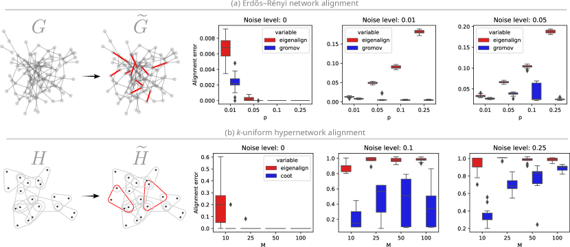
Figure 2: (a) Illustration of Erdös-Rényi random graph alignment problem with noise; alignment errors achieved by EigenAlign and Gromov-Wasserstein under permutation and noise. (b) Illustration of random 3-uniform hypergraph alignment problem with noise; alignment errors achieved by higher-order EigenAlign and COOT under permutations and noise.

For this first set of experiments, we use synthetic datasets of graphs and hypergraphs. In Figure 2(a) we investigate the relative performance of spectral alignment and Gromov-Wasserstein alignment, considering Erdös-Rényi (ER) graphs of size $N=100$ with parameter $p\in\{0.01,0.05,0.1,0.25\}$. For a randomly sampled ER graph $G$, we form a copy $\widetilde{G}$ in which vertices have been relabeled via a random permutation. Optionally, we also add noise in the form of random addition or deletion of edges independently with probability $q\in\{0,0.01,0.05\}$. We align $G$ to $\widetilde{G}$ using both the implementation of EigenAlign from [25] and Gromov-Wasserstein using a proximal gradient algorithm (see Algorithm 3), similar to the approach taken by [69]. Since the proximal gradient algorithm yields a coupling that is dense but potentially vanishingly small for most entries (i.e. strictly on the interior of the constraint set), we apply a “rounding” of the result onto an extreme point of the coupling polytope to yield a sparse permutation matrix. For each alignment, we calculate the corresponding distortion functional (1) to measure the alignment quality. In the absence of noise, $\widetilde{G}$ and $G$ are isomorphic since they are represented by adjacency matrices that are identical up to permutation, and a distortion of zero corresponds to a perfect matching. Non-zero noise breaks this isomorphism (so that the ground truth vertex matching may no longer be the “right” one after adding noise), so the lower the distortion the better the alignment. In this sense, the distortion is an objective measure of alignment quality rather than the coupling itself. In all cases we consider, we find that Gromov-Wasserstein finds an alignment that yields a lower distortion than EigenAlign, shown in Figure 2 (a). At a conceptual level, this can be understood since the Gromov-Wasserstein problem arises as a relaxation of the quadratic assignment problem (36) that accounts for the quadratic objective and the assignment constraints jointly, whereas the EigenAlign approach adopts a two step approach, first relaxing the assignment constraint to a norm ball constraint (37) and then projecting back onto the assignment polytope (38). Because of this, the assignment constraints in the second step cannot inform the quadratic program in the first step.

In Figure 2(b) we turn to hypergraph alignments. For hypergraphs, the scope of the higher-order spectral alignment approach is limited to dealing with uniform hypergraphs, and furthermore the time and space complexity scale exponentially in the order of the hypergraph. We therefore consider random 3-uniform graphs for $N=25$ vertices and $M=\{10,25,50,100\}$ hyperedges. Each hyperedge is obtained by sampling 3 vertices uniformly without replacement from the vertex set. Given a hypergraph $H$, we form a copy $\widetilde{H}$ by randomly relabeling vertices and hyperedges, and then replacing a fraction $q\in\{0,0.1,0.25\}$ of hyperedges with independently sampled hyperedges. The spectral alignment approach only aligns vertices (since for uniform hypergraphs a vertex alignments also induces hyperedge alignments), so we quantify the quality of alignments in terms of the objective of (39) rather than the co-optimal transport distortion which depends on both vertex and hyperedge couplings. As in the graph alignment case, we find that co-optimal transport alignments (using again the proximal method of Algorithm 3) perform as well or better compared to spectral alignments in all cases.

Spectral hypergraph alignments are restricted to uniform hypergraphs and are computationally expensive, while co-optimal transport does not have these limitations. Measuring the computation time for spectral alignment and co-optimal transport alignment for $N\in\{5,10,25\}$, we find that spectral alignment is several orders of magnitude more expensive in terms of runtime. Runs for $N=50$ with spectral alignment failed due to memory usage exceeding the available 32 GB.

5.2.2 Metabolic network alignment

Metabolic networks (and chemical reaction networks more generally) are an example of systems in which higher-order relations are essential to retain information: chemical species may be modeled as vertices and reactions as hyperedges, which may involve any number of reactants simultaneously [28]. We consider the metabolic networks of E. coli and halophilic archaeon DL31, retrieved from the Kyoto Encyclopedia of Genes and Genomes (KEGG) database [29] with accession numbers eco01100 and hah01100 respectively. We model each metabolic network as a labeled measure hypernetwork, where vertices are identified with metabolite compounds and hyperedges are identified with enzymes which catalyze reactions involving multiple compounds (multiple reactants and products). For simplicity, we discard directionality information and model the metabolic networks as undirected hypergraphs (i.e. we do not distinguish between reactants and products within each hyperedge). For eco01100 (the source network) we construct a measure hypernetwork with 984 metabolites and 1005 reaction terms, and for hah01100 (the target network) a measure hypernetwork with 679 metabolites and 558 reaction terms. We find that the minimum and maximum hyperedge sizes are 2 and 9, respectively, in both the source and target hypergraphs. This verifies the heterogeneous, non-uniform nature of these hypernetworks. We visualize each network in Figure 3(a), showing the associations between compounds (vertices, red) and reactions (hyperedges, blue). In contrast to the previous synthetic example, we now must align two hypergraphs that are non-uniform and different in size. Within our framework, the unbalanced, fused hypergraph alignment scheme is the most suitable approach and we demonstrate the effectiveness of this method.

This hypergraph alignment problem was addressed using a spectral approach by [50], in which input hypergraphs are represented as adjacency tensors, and higher-order power iterations are employed for spectral alignment as described in Section 5.2.1. As the metabolic hypernetworks are non-uniform, dummy vertices are added to produce a $d$-uniform hypergraph where $d$ is the maximum hyperedge degree in the original non-uniform hypergraph. This uniform hypergraph is then represented as a $|V|^{d}$ adjacency tensor. For uniform hypergraphs of even moderate size, the computational burden of this approach becomes extreme as the memory requirements for storing the adjacency tensor grow exponentially with the degree. Indeed, in [50] a fairly involved computational scheme is described that exploits the supersymmetry of the alignment tensor. Even so, distributed computing is necessary to speed up the alignment, which was reported to take over two hours to match the two networks (559 metabolites and 537 reactions for hah01100, 794 metabolites and 923 reactions for eco01100) [50, Supplementary materials].

For metabolite compounds and reaction terms, we construct pairwise cost matrices between the source and target using a similar approach to [50]. For metabolites, similarity scores are calculated using the cheminformatics package ChemmineR [11]. For any two enzymes $(e_{1},e_{2})$, the similarity score is taken to be $1/N(e_{1},e_{2})$ where $N(e_{1},e_{2})$ is the number of enzyme entries in the lowest common level in the Enzyme Commission (EC) classification. We then perform unbalanced, fused hypergraph alignment between the two hypernetworks using a proximal point variant of Algorithm 5, using $\alpha=0.9,\varepsilon=10^{-3},\lambda=0.1$ and 250 and 1000 inner and outer iterations respectively. This takes less than a minute utilizing 4 cores of an Intel Xeon Gold 6242 system, several orders of magnitude faster than the higher-order spectral method employed by [50].

To assess the quality of the matching, we use the fact that compounds and enzymes conserved between these two organisms are known. For a subset of vertices and hyperedges therefore, we have a biological “ground truth” correspondence to compare against. Since only parts of the two metabolic networks are shared, we expect the unbalanced matching to reflect this and assign more mass to shared components. In Figure 3(b) we show reactions and compounds in each organism, ranked by the (log) total mass assigned to it by the unbalanced matching algorithm. Components which have a true match in the target network are shown in green – it is clear that more mass is assigned to components with a true match, and non-overlapping components tend to be downweighted. These weights can be thought of as a measure of confidence in the alignment. We remark that the eco01100 network is larger, so a significant fraction of its components do not have true matches in the hah01100 network. Despite this, we still observe a separation in hah01100 between components with and without true matches.

To understand how our alignment method depends on the node and hyperedge labels and relational information encoded in the hypergraph structure, we perform two additional alignments where some of this information is hidden. To study the performance of alignment using hyperedge label information alone without the hypergraph structure, we directly align enzymes (hyperedges) using the enzyme similarity matrix by solving a standard optimal transport problem using the proximal point method [66]. We also consider hyperedge alignment using vertex labels and the hypergraph structure, when hyperedge labels are hidden. To do this, we set the hyperedge-hyperedge cost matrix to zero and recompute the alignment with the same parameters using only the vertex-hyperedge incidence matrix and the vertex-vertex cost matrix. In Figure 3(c), for the subset of enzymes / reaction terms shared between both organisms, we show alignments obtained using only hyperedge labels (enzyme similarity), the full labeled hypergraphs (hypergraph), and only vertex labels (hypergraph, ablated). Compared to the full labeled hypergraph alignment result, we find that using only enzyme similarity leads to a much more noisy alignment, with large amounts of mass assigned away from the diagonal. Suppressing hyperedge labels leads to a slightly worse alignment of hyperedges compared to the full labeled alignment, but still significantly cleaner than using hyperedge labels alone.

Finally, we focus on the tricarboxylic acid (TCA) cycle, a fundamental metabolic process that is conserved between both organisms. In Figure 3(d) we highlight this subnetwork, and in Figure 3(e) we show its rubber band visualization. In Figure 3 (f), we find that a full labeled hypergraph alignment near-perfectly matches the components, while the ablated hypergraph alignment without hyperedge labels again does slightly worse. In contrast, the enzyme similarity score does not provide full information about the matching, and hence alignment based on enzyme similarity alone performs much worse. Together, these results indicate that utilizing the hypergraph structure in combination with label information is crucial for achieving a good alignment between the two metabolic networks, outperforming alignments where either label or relational information are suppressed.

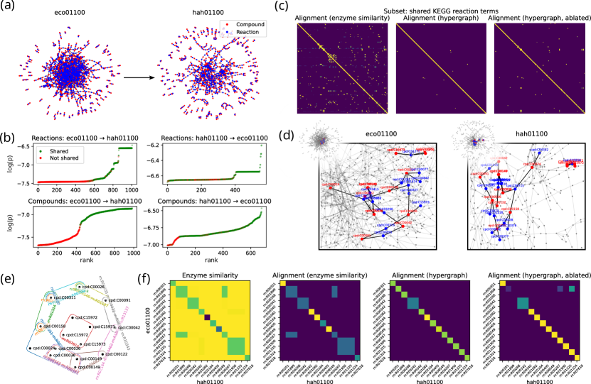
Figure 3: (a) Genome-scale metabolic networks of E. coli (eco01100) and halophilic archaeon DL31 (hah01100). (b) Vertices (compounds) and hyperedges (enzymes) ranked by total out-going probability mass as found by unbalanced alignment, colored by whether its true match is shared in the target network. (c) Hyperedge couplings for the subset of reaction terms (enzymes) common to both organisms, found using (i) enzyme similarity only, (ii) labeled hypergraph alignment (with both metabolite and enzyme similarities provided), and (iii) ablated, labeled hypergraph alignment (with metabolite similarities provided, but not enzyme similarities). (d) Zoom-in on conserved tricarboxylic acid (TCA) cycle subnetwork as shown in genome-scale metabolic network layout from (a). (e) Hypergraph layout of TCA cycle subnetwork, shown as a rubber band diagram. (f) Alignment of reaction terms in TCA cycle subnetwork: (i) enzyme similarity matrix for TCA cycle reaction terms, and alignments found using (ii) enzyme similarity, (iii) labeled hypergraph alignment (with both metabolite and enzyme similarities provided), (iv) ablated labeled hypergraph alignment (with metabolite similarities provided, but not enzyme similarities).

5.2.3 Multi-omics sample and feature alignment

Co-optimal transport has previously been employed for simultaneously matching samples and features between heterogeneous datasets [59]. One particularly popular example is that of multi-omics datasets, where two or more sets of features (e.g. gene expression and protein marker expression) are observed in samples (cells) [60]. This problem can be cast in the setting of hypernetwork alignment by interpreting samples and features as vertices and hyperedges respectively, and the sample-by-feature data matrix as the membership function. In [60] the application of unbalanced co-optimal transport was demonstrated to improve alignment quality, and in [23] the augmented Gromov-Wasserstein matching (see Definition 6) is introduced: this corresponds to partitioned network matching when only vertex-vertex information is provided in addition to vertex-hyperedge relations, but not hyperedge-hyperedge information. Here we consider 1,000 cells sampled from the same CITE-seq dataset as in [23], in which 15 genes and their corresponding marker proteins were measured.

Partitioned measure networks allow pairwise relations within, as well as between, partitions to be modeled, so we incorporate pairwise similarities in each domain. This is in addition to the sample-feature information contained directly in the data matrix. We choose to capture this by calculating sample-sample and feature-feature correlations. Under the partitioned measure network alignment framework, we expect that pairwise structure between samples (features) should be preserved by the alignment. To get an initial understanding of the data, we show the PCA embeddings and the partitioned network data constructed from each modality in Figure 4(a): $\omega_{00}^{(\mathrm{RNA},\mathrm{ADT})},\omega_{11}^{(\mathrm{RNA},\mathrm{ADT})}$ are correlation matrices between samples and features respectively, and $\omega_{01}^{(\mathrm{RNA},\mathrm{ADT})}$ are the data matrices capturing cell-wise gene or marker expression. Put simply, we expect that correlated (anticorrelated) pairs of genes should be matched to correlated (anticorrelated) pairs of proteins, and similarly for cells between modalities.

We then compute an entropy-regularized alignment of the RNA and protein partitioned measure networks using Algorithm 4. We introduce a parameter $\alpha\in[0,1]$ to control the trade-off between the contribution of Gromov-Wasserstein type terms ($\omega_{00},\omega_{11}$) and co-optimal transport type terms ($\omega_{01}$), scaling these inputs by $\sqrt{\alpha}$ and $\sqrt{1-\alpha}$ respectively. We choose values $\alpha\in\{0,0.1,\ldots,0.9,1\}$. For each partition, different levels of entropic regularization $\varepsilon_{0,1}\in\{\texttt{5e-4},\texttt{1e-3},\texttt{5e-3},\texttt{1e-2},\allowbreak\texttt{5e-2},\texttt{0.1},\texttt{0.5}\}$ are used, as it is well known that regularization level may play a role in the alignment quality [23]. Finally, we consider the special cases where pairwise information (i.e. the Gromov-Wasserstein term) on samples, features, or both, are suppressed. We implement this by setting $\omega_{00}^{\mathrm{RNA},\mathrm{ADT}}$, $\omega_{11}^{\mathrm{RNA},\mathrm{ADT}}$ to zero as needed.

For each set of parameter values we compute the alignment, and then calculate the fraction of gene transcripts which are correctly matched to their corresponding protein in terms of maximum assigned probability. We show in Figure 4(b) the best matchings obtained for the settings of partitioned matching, co-optimal transport, and augmented Gromov-Wasserstein (AGW) with pairwise samples on samples and features respectively. In terms of identification of features (Figure 4(c)), we found that the partitioned alignments and AGW with sample-sample information were both able to correctly assign 13/15 (87%) features, in terms of maximum probability. On the other hand, AGW with feature-feature information and co-optimal transport correctly assigned 8/15 and 6/15 features respectively. While the fraction of correctly matched features by maximum probability gives an indication of the alignment accuracy, it does not account for the level of uncertainty in the matching. To account for this, we also calculate the KL divergence of the diagonal (ground truth) coupling relative to the alignment, reasoning that alignments that produce the correct matching with a higher certainty should have a lower divergence. We find that the partitioned matching produces a more informative alignment ($\operatorname{KL}=0.502$) compared to AGW ($\operatorname{KL}=1.027$), which can also be assessed visually from the couplings. Finally, in Figure 4(c) bottom plot, we assess the quality of sample matchings in terms of the fraction of samples closer than true match (FOSCTTM) which is a standard performance metric in the single cell alignment literature [23], for which a lower value indicates a better alignment. Both the partitioned alignment and AGW with sample-sample information produce sample alignments of similar quality, while AGW with feature-feature information and co-optimal transport do worse.

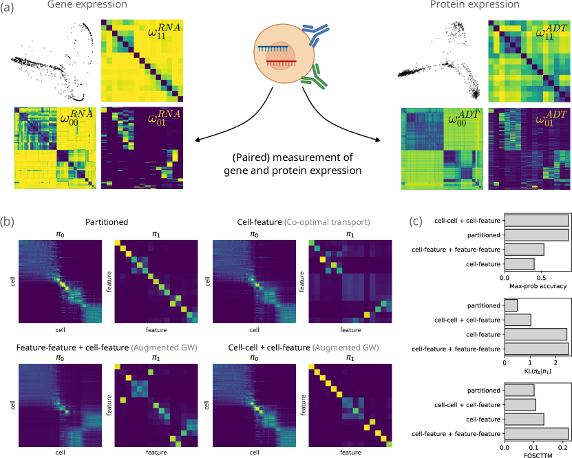
Figure 4: (a) Illustration of CITE-seq dataset shown in transcriptomic (RNA) and surface marker (ADT) modalities. For modality $m$, $\omega_{01}^{m},\omega_{00}^{m},\omega_{11}^{m}$ denote the data matrix, sample-sample similarities, and feature-feature similarities. (b) Sample and feature alignments obtained using partitioned network matching, co-optimal transport, and augmented Gromov-Wasserstein with sample-sample information and feature-feature information respectively. The ground truth matching for samples and features corresponds to the diagonal. (c) Quality of feature alignments in terms of (i) maximum probability assignment (higher is better) and (ii) reverse KL-divergence to the diagonal coupling (lower is better). (iii) Quality of sample alignments in terms of FOSCTTM (lower is better).

5.3 Partitioned networks for multiscale network matching

While the previous examples have focused on hypergraphs, i.e. partitioned networks with $k=2$, for $k\geq 2$ our framework can be used to model multiscale data. This insight was pointed out in [20]: a multi-scale graph with $k$ simplification levels can be modeled as $k$ coupled hypergraphs. In Section A.6, we show how this can in fact be framed and extended in terms of $k$-partitioned measure networks. Specifically, the partitioned networks approach allows us to model relations between vertices in the same simplification level, as well as between simplification levels. We demonstrate the application of this method both for matching geometric networks (obtained from point cloud data), as well as non-geometric protein-protein interaction networks.

5.3.1 Multiscale point cloud matching

We apply multiscale matching to networks derived from 3D models of a wolf and a centaur from the TOSCA object database [9]. In [20], co-optimal transport was employed to find semantic matchings between two poses of the centaur graph across multiple scales. In their experiments, the two poses of the centaur graph had the same number of nodes at each level and were nearly identical in structure. We address the much more challenging problem of finding semantic matchings between a wolf and a centaur, where the two graphs are significantly different in their sizes, connectivities, and semantic components. Indeed, the “true” semantic correspondence between the objects is not one-to-one, since the wolf has four limbs and the centaur has six.

For each input graph, a multi-scale topological simplification was produced using the heat kernel multiscale reduction of [20, Section 5.3] with $k=3$ simplification levels. We take each of the $\omega_{i,i+1},\omega_{i,i+1}^{\prime}$, for $0\leq i<2$ to be binary incidence matrices of vertex-hyperedge relations between successive reductions. Pairwise relations $\omega_{ii},\omega_{ii}^{\prime},0\leq i<3$ are constructed from the graph shortest path distances on each simplification level.

In Figure 5 we visualize the alignments obtained using multiscale COOT (using the algorithm of [20]), Gromov-Wasserstein independently on each simplification level, the multiscale alignment using $k$-partitioned networks (Algorithm 4) and its unbalanced variant (Algorithm 6). At each simplification level, each vertex in the centaur graph is connected to a vertex in the wolf graph with the maximum matching probability. While multiscale COOT finds a matching that is largely consistent across scales, the matching is very noisy especially at fine scales as evidenced by discontinuities in the color gradient in the centaur. On the other hand, independent Gromov-Wasserstein matchings of each simplification leads to more locally consistent matchings (continuous color gradients), but the matching fails to be consistent between scales: this is apparent by looking at the matchings of the head/neck regions across simplification levels (blue arrows), as well as the arms of the centaur, for instance. The multiscale partitioned network alignment produces a semantically reasonable, consistent matching at each scale, correctly matching the head, neck, hind legs, as well as tail regions. Due to the difference in the number of limbs across each model, the mis-matching of the arms of the centaur is not entirely surprising. Interestingly, a small portion of the front legs of the centaur model is matched to the hind legs of the wolf (red arrows), seen as a discontinuity in the color gradient. This disappears in the unbalanced partitioned alignment, suggesting that the cause is the lack of one-to-one correspondence between the two structures, and that allowing for unbalanced matchings may alleviate this.

In addition to the visual assessment of semantic matchings, we show in Table 1(a) different components of the objective (71) for the matchings found by Gromov-Wasserstein, partitioned alignment, and multiscale COOT. This provides us with an unbiased quantification of alignment quality directly in terms of the distortion. These results confirm our visual observations from Figure 5: Gromov-Wasserstein alignment at each scale produces the minimal GW loss reflecting preservation of pairwise relations at each individual scale, but a very high COOT loss indicating a lack of consistency across scales. Conversely, multiscale COOT minimizes the COOT loss while producing the highest GW loss, which suggests the reverse. The partitioned alignment on the other hand yields a much lower GW loss, while achieving a COOT loss only marginally worse than that found by multiscale COOT. These results demonstrate that the partitioned multiscale alignment is able to incorporate both pairwise and multiscale information effectively to simultaneously align networks at multiple scales.

Figure 5: Multiscale network matchings: TOSCA wolf and centaur. Each row corresponds to a different algorithm, and each column corresponds to a graph simplification level. Blue arrows: matching of the wolf’s head is inconsistent across scales for Gromov-Wasserstein alignment. Red arrows: discontinuity in centaur’s front leg disappears with an unbalanced alignment.

	COOT_loss	GW_loss
Gromov-Wasserstein	0.036033	0.010600
Multiscale COOT	0.018261	0.019294
Partitioned alignment (projected gradient)	0.019534	0.012787

(a) TOSCA wolf and centaur: COOT and GW distortion losses.

Method	COOT_loss	GW_loss	Node correctness	Edge correctness
Gromov-Wasserstein	0.058684	0.016181	0.613546	0.967680
Multiscale COOT	0.028927	0.021701	0.036853	0.565782
Partitioned (proximal)	0.030732	0.016125	0.585657	0.964916
Partitioned (block)	0.032357	0.014105	0.597610	0.951580

(b) Protein-protein interaction subnetwork: COOT and GW distortion losses, as well as node and edge correctness.

Table 1: Gromov-Wasserstein (GW) and co-optimal transport (COOT) loss values for multiscale network matching.

5.3.2 Multi-scale biological network matching

Our multi-scale network matching approach is not limited to geometric graphs, i.e. ones constructed from a point cloud. To demonstrate this, we consider a dataset of protein-protein interaction (PPI) networks [63], in which nodes and edges correspond to protein species and biochemical interactions respectively. We take $G_{0}$ to be the PPI network of high-confidence interactions among 1,004 proteins, and $G_{0}^{\prime}$ to be the PPI network with 20% more low-confidence interactions. For each of $G_{0},G_{0}^{\prime}$ we construct a progressive topological simplification again using the heat kernel reduction described in [20], yielding multi-scale reductions $\{G_{i}\}_{i=0}^{2}$ and $\{G_{i}^{\prime}\}_{i=0}^{2}$. We visualize in Figure 6(a) each multiscale reduction, in which nodes are colored by the leading non-trivial eigenvector of $L_{G_{0}}$, the graph Laplacian of $G_{0}$. Nodes in the low-confidence networks $G_{0}^{\prime}$ are also colored using the ground truth node correspondence. We then calculate matchings at each scale by employing partitioned alignment, multiscale co-optimal transport, as well as independent Gromov-Wasserstein matchings at each simplification level. For the partitioned alignment as well as Gromov-Wasserstein, we used a proximal gradient algorithm (Algorithm 3). In Figure 6(b) the matchings from each of these algorithms are shown across all three simplification levels. We also show a set of “ground truth” couplings: between $G_{0}$ and $G_{0}^{\prime}$ this is the identity coupling, while between $G_{i}$ and $G_{i}^{\prime}$ for $i=1,2$ an approximate ground truth coupling is found by calculating a matrix of pairwise correlations between coarse-grained nodes and then solving a linear assignment problem. From a visual assessment of each of the matchings, we observe that both the partitioned alignment and Gromov-Wasserstein find matchings between $G_{0}$ and $G_{0}^{\prime}$ that resemble the ground truth, while multiscale COOT performs quite poorly: this reflects the fact that multiscale COOT is unaware of the pairwise adjacency information at each scale. Between $G_{1}$ and $G_{1}^{\prime}$, we find that the partitioned alignment continues to resemble the ground truth, but both Gromov-Wasserstein and multiscale COOT matchings begin to deviate significantly. Finally, between $G_{2}$ and $G_{2}^{\prime}$, we find that Gromov-Wasserstein continues to appear very different from the ground truth.

Due to the non-geometric nature of the input graphs, an effective direct visualization of the matchings is very difficult. To demonstrate the difference in matching results in a clearer way, we employ the Louvain community detection algorithm [6] which finds a partitioning of $G_{0}$ (and hence $G_{0}^{\prime}$) into $m=12$ communities. Together with the hypergraph coupling between simplification levels $i$ and $i+1$, the matching $\pi_{i}$ at simplification level $i$ induces a matching of communities. In Figure 6(c) we show the induced community matchings for each alignment method, as well as for the ground truth. At level 0, the partitioned alignment and Gromov-Wasserstein both produce nearly perfect alignments, while multiscale COOT performs poorly. At level 1 however, both Gromov-Wasserstein and multiscale COOT perform poorly, while partitioned alignment continues to perform well. Finally, at level 2 from the ground truth matching it is apparent that too much information is lost by coarse graining to correctly identify communities. However, the matching induced by the partitioned alignment is still closer to the ground truth, for instance in L1 norm (L1 = 0.265) compared to Gromov-Wasserstein (L1 = 0.319) and multiscale COOT (L1 = 0.508).

In Table 1(b) we show the loss terms similar to the previous TOSCA example: we observe that Gromov-Wasserstein fails to find consistent matchings across scales as evidenced by a high COOT loss. On the other hand, multiscale COOT leads to poor preservation of pairwise relations within each simplification level, indicated by a high GW loss. In contrast, partitioned alignments are able to find multiscale matchings that are consistent within each scale as well as across scales. Furthermore, partitioned alignment methods yield node and edge correctness scores for level 0 that are comparable to Gromov-Wasserstein, which was found to outperform most other competing alignment methods in [68].

Figure 6: Multiscale matchings for protein-protein interaction networks: (a) Network layouts of successive simplifications $\{G_{i}\}$ and $\{G_{i}^{\prime}\}$ for $i=0,1,2$ with nodes colored by the leading nontrivial eigenvector of $L_{G}$. (b) Matchings found at each scale using (i) partitioned matchings, (ii) multiscale COOT (iii) Gromov-Wasserstein at each level, and (iv) the ground truth matching. (c) Matchings of Leiden communities induced by the node-level matching between $G_{i}$ and $G_{i}^{\prime}$ at each simplification level $i$. “Ground truth” shows the best possible matching of Leiden communities using couplings at this level of granularity.

5.4 Geodesics and Fréchet means

In Section 4.3, we introduced the Fréchet functional (26) on the space of partitioned measure networks and calculated its gradient. Recalling from Theorem 15 that the spaces of measure networks and measure hypernetworks isometrically embed into the space of partitioned measure networks, we recover from (26) the Fréchet functional on measure networks [18, 43] and measure hypernetworks [20] as special cases. For simplicity we consider the unlabeled case here, although in general our results can be straightforwardly extended to measure networks with labels valued in an inner product space (see e.g. [65]).

In practice, a stationary point of the functional (26) can be found via gradient descent on the space of partitioned measure networks using the “blow-up” scheme of [18] which progressively carries out alignment of network representatives as per Proposition 53. This approach exploits the empirical observation that optimal couplings of measure networks tend to be sparse (see e.g. [18, Appendix C] and [19, Theorem 2]), allowing the geodesics of Proposition 33 to be explicitly constructed. While the approach of [18] handles only measure networks, we implement an extension of [18, Algorithms 1-3] in order to handle measure hypernetworks. We remark here that, although the question of sparsity of optimal couplings is open in the general quadratic case, in the setting of co-optimal transport between measure hypernetworks the alternating scheme of Algorithm 1 is guaranteed to yield a sparse coupling. This is because each iterate is the solution of a linear program and is therefore sparse. In what follows, we refer to this approach as the free support method, since the size of the networks is determined as part of the optimization procedure.

As an alternative to the more involved free support method, we also consider fixing the networks to those described by matrices of a fixed size. This makes the optimization much easier: as detailed in Section A.7, this can be solved by alternating between solving independent alignment problems and a closed form update for the barycenter. We refer to this approach as the fixed support method.

In Figure 7(a) we take three hypergraphs $H_{0},H_{1},H_{2}$ shown as “rubber-band” diagrams in which vertices are represented as points, and hyperedges are shown as “rubber bands” around the convex hull of contained vertices. We interpolate between these hypergraphs by computing the Fréchet means of $\{H_{0},H_{1},H_{2}\}$ with various weights $(w_{0},w_{1},w_{2})$, using both the free support and fixed support methods. Since the rubber band visualization is unable to represent weighted vertex-hyperedge relationships, a threshold (in this case we chose $\omega(x,y)>1/4$) is applied to the membership function $\omega(x,y)$ before visualization. As a result, Figure 7(b) cannot reflect the true nature of the interpolation in the measure hypernetwork space. In Figure 7(c) we show the interpolated function $\omega$, making the interpolation readily apparent. We remark that the size (number of vertices and hyperedges) of each interpolating measure hypernetwork is determined by the blowup scheme (in general, larger than each of the inputs), and that the ordering of rows and columns in the visualization is arbitrary. In Figure 7(d) we show the membership functions of barycenters computed using the fixed support method. We note a close resemblance between the results of the free and fixed support approaches.

Finally, in Figure 7(e) we compute the measure hypernetwork distance (per Definition 6) from each interpolated hypernetwork to each input hypernetwork. For true interpolations we would expect the distance to vary affinely across the simplex. However, in the case of free support barycenters we observe that is not always the case. This suggests that local minima may have played a role in the calculation of the weighted Fréchet means or also calculating the distances to each endpoint, reflecting the non-convex nature of the distance and alignment computation. On the other hand, for fixed support barycenters we recover the expected trend. This reflects the computationally simpler nature of the fixed support method, and may indicate that the fixed support barycenters are more accurate representations of the true hypergraph barycenter.

Figure 7: Geodesic interpolations between three hypergraphs $H_{0},H_{1},H_{2}$, shown in (a) as “rubber-band” diagrams. Interpolations found using the free-support method are visualized in (b) as rubber band diagrams and also directly as their membership functions $\omega$ in (c). (d) Fixed support (using $32\times 32$ matrices) interpolations visualized as membership functions. (e) Hypergraph distance $d_{\mathcal{H},2}(H_{i},H_{\mathrm{interp}})$ between each of the three input hypergraphs and geodesic interpolations, both for the free support and fixed support barycenters.

Figure 8: (a) Learned dictionary weights for each interpolation instance using linear dictionary learning (correlation = 0.894) and geodesic dictionary learning (correlation = 0.809), compared to the true weights. (b) Measure hypernetwork distances between true networks and dictionary learning reconstructions, under random permutation of dictionary elements. (c) Atoms learned by linear dictionary learning. (d) Atoms learned by geodesic dictionary learning.

5.5 Linear and non-linear dictionary learning

We may extend the barycenter question and ask for several characteristic partitioned measure networks that best describe an ensemble of partitioned measure networks, rather than a single barycenter or Fréchet mean. One common method is to learn a small basis of archetypes, such that each datapoint can be approximated by a convex combination of these archetypes. Also known as dictionary learning, this has become a classical analysis approach for vector-valued data [33] and recently has been extended to graph-valued data [65, 67] using the Gromov-Wasserstein framework. We extend this to the general case of partitioned measure networks, which also covers the settings of measure networks and measure hypernetworks.

5.5.1 Nonlinear (geodesic) dictionary learning

For a collection of $N$ $k$-partitioned measure networks $P_{i}=\big{(}X_{i},\mu_{i},\omega_{i}\big{)}\in\mathcal{P}_{k},1\leq i\leq N$, the geodesic dictionary learning problem is

$$\min_{\{D_{j}\}_{j=1}^{m}\in\mathcal{P}_{k},\{\alpha_{i}\}_{i=1}^{N}\in\Delta^{m}}\frac{1}{N}\sum_{i=1}^{N}d_{\mathcal{P}_{k},2}\left(B(\mathcal{D},\alpha_{i}),P_{i}\right)^{2},$$ (40)

where $B(\mathcal{D},\alpha)$ is the barycenter operator (28) for a collection $\mathcal{D}=\{D_{i}\}_{i=1}^{m}\in\mathcal{P}_{k}$ of partitioned measure networks and $\alpha\in\Delta^{m}$ are the corresponding coefficients. We derived the gradients of this function in Section 4.3.2. Like related methods [48, 70], this is a non-convex, bilevel minimization problem which is not straightforward even to find a local optimum. While problems of this nature can be solved using more involved schemes such as [67], we propose to find a local minimum solution for dictionary networks of fixed size by a simple gradient descent.

5.5.2 Linear dictionary learning

Solution of the bilevel problem (40) for geodesic dictionary learning is computationally demanding due to the computation of the barycenter operator at each iteration. As an alternative, linear dictionary learning approaches have been proposed [65, 46], in which the (Fréchet) barycenter operator $B(\mathcal{D},\alpha)$ is replaced with its Euclidean equivalent, a weighted superposition of the atoms $\mathcal{D}[\alpha]=\sum_{j=1}^{m}\alpha_{j}\omega_{\mathcal{D}_{j}}$. Since reconstructions from the dictionary are carried out in the Euclidean space, this eliminates the nested optimization arising from the barycenter computation, at the cost of departing from the natural geodesic structure of the space of (partitioned) measure networks. We remark that in the setting where the data $P_{i}\in\mathcal{P}_{k},1\leq i\leq N$ are sufficiently close together (in the sense of the injectivity radius of the exponential map), that linear dictionary learning is equivalent to the nonlinear case.

The linearized equivalent of (41) is

$$\min_{\{\omega_{D_{j}}\}_{j=1}^{m}\in L^{2}(X^{2},\mu^{\otimes 2}),\>\{\alpha_{i}\}_{i=1}^{N}\in\Delta^{m}}\frac{1}{N}\sum_{i=1}^{N}d_{\mathcal{P}_{k}}\left(\mathcal{D}[\alpha_{i}],P_{i}\right)^{2},$$ (41)

where for brevity we have denoted the linear combination of atoms in $\mathcal{D}$ with coefficients in $\alpha$ to be

$$\mathcal{D}[\alpha]=\left(X,\mu,\sum_{j=1}^{m}\alpha_{j}\omega_{D_{j}}\right)\in\mathcal{P}_{k}.$$

In this formulation, we ask for $m\ll N$ atoms $\{\omega_{D_{j}}\}_{j=1}^{m}\in L^{2}(X^{2},\mu^{\otimes 2})$ and for each input network $P_{i}$ a corresponding set of coefficients $\{\alpha_{ij}\}_{j=1}^{m}$ such that the reconstructed network described by incidence matrix $\mathcal{D}[\alpha_{i}]$ is close to $P_{i}$ in the sense of the optimal transport metric. In the above, we fix the partitioned measure space to $(X,\mu)$ respectively. We note that the computation of $d_{\mathcal{P}_{k}}$ involves solution of a nonlinear program for the coupling $\pi$. We can expand the $d_{\mathcal{P}_{k}}$ terms within the objective (41):

$$\min_{\{\omega_{D_{j}}\}_{j=1}^{m},\{\alpha_{i}\}_{i=1}^{N},\{\pi_{i}\in\Pi_{k}(\mu,\mu_{i})\}_{i=1}^{N}}\frac{1}{N}\sum_{i=1}^{N}\left\langle L\left(\mathcal{D}[\alpha_{i}],\omega_{P_{i}}\right),\pi_{i}\otimes\pi_{i}\right\rangle.$$ (42)

Minimizing in $\pi_{i}$ can be done independently and in parallel for each of the $1\leq i\leq N$ inputs. Fixing $\pi$, we have a non-convex quadratic program in the atoms $\omega_{D_{j}}$ and the coefficients $\alpha_{i}$. We solve the problem (41) using a stochastic projected gradient descent.

To try this out, we consider again the example from Section 5.4 in which three hypergraphs were given. We generated barycenters of these three hypergraphs with mixture weights uniformly spaced across a barycentric grid using the “blow-up” algorithm. This produced an ensemble of 45 hypergraphs in which the number of vertices ranged from 6 to 23, and the number of hyperedges between 4 and 17. By construction, the input hypergraphs $H_{0},H_{1},H_{2}$ are the ground truth atoms, and weights $\{w_{ij}\}_{1\leq i\leq N,0\leq j\leq 2}$ serve as the ground truth mixture coefficients. In Figure 8(a) we show the dictionary weights learned by the linear and geodesic dictionary learning respectively, compared to the true weights. Although geodesic dictionary learning (at least in theory) accounts correctly for the underlying geometry of hypergraphs, we find that linearized dictionary learning yields better results in practice. A potential explanation for this result is that linearization avoids the need to solve a non-convex inner loop problem, replacing this with Euclidean averaging.

To illustrate what we gain by using geodesic over linearized dictionary learning, for each method we randomly permute the learned dictionary atoms and re-calculate the reconstruction error. We show in Figure 8(b) the reconstruction error across 10 independent permutations. In the space of measure hypernetworks, this amounts to changing the choice of representative for the dictionary atoms. This leads to an increased reconstruction error for linearized dictionary learning, relative to geodesic dictionary learning: this tallies with geodesic dictionary learning objective being defined independent of choices of representative. Overall, we find that linearized dictionary learning has an advantage over its geodesic variant due to computational simplicity, and this is the algorithm we use in the following sections.

Finally, we show in Figure 8(c, d) the atoms learned by linear and geodesic dictionary learning respectively: note that both methods are able to reliably reconstruct the atoms shown in Figure 7(a), which were used to generate the input ensemble.

5.5.3 Example: stochastic block model

For a further validation of our approach using synthetic data, we devise a simple generative model for random non-uniform hypergraphs that is analogous to the stochastic block model in the case of simple graphs, similar to the model that was introduced in [24]. For a (possibly random) number of vertices $|V|$ and given a fixed number of blocks $k$, we partition the vertex set $V$ into $k$ blocks of size $\lfloor|V|/k\rfloor$, with one block containing any remainders. A random number, $|E|$, of hyperedges are then sampled. With probability $p$, a sampled hyperedge will span $m<\lfloor N/k\rfloor$ vertices, all residing in one of the $k$ blocks chosen uniformly at random. Otherwise the hyperedge will consist of $m$ vertices sampled uniformly from all vertices in $V$. The key parameters at play here are thus $k$ and $p$, respectively controlling the number of blocks and the level of noise present.

We set up three block models with $k=2,3,4$ blocks and $p=2/3$, from each of which 50 hypergraphs are sampled. For each hypergraph, the number of vertices and hyperedges are chosen uniformly on $[16,32]$ and $[24,32]$ respectively. We show examples of sampled hypergraphs for each $k$ in Figure 9(a). We apply both linearized and geodesic hypergraph dictionary learning (HDL) algorithms to this dataset of 150 hypergraphs to learn $3$ atoms.

For comparison to graph-based methods, we apply the graph-based dictionary learning method of [65] using flattened hypergraphs obtained by taking the sum $\frac{1}{|E|}\sum_{i=1}^{|E|}\mathbf{1}_{e_{i}}\mathbf{1}_{e_{i}}^{\top}$, that is, putting a weighted connected component in place of each hyperedge (see Figure 9(b)). As can be seen from the learned atoms and coefficients in Figure 9(c-d), HDL is able to accurately learn distinct atoms corresponding to different values of $k$. By comparison, graph dictionary learning finds atoms that appear to be mixed.

We use the learned coefficients from HDL and GDL as features for support vector machine (SVM) classification. In Figure 9(e) we show the accuracy in 10-fold cross validation for both (linear and geodesic) hypergraph and graph dictionary learning. For comparison, we also show accuracies achieved by two commonly used graph kernels, the Weisfeiler-Lehmann isomorphism test and the shortest path kernel [52], applied to the flattened hypergraphs. We find that both variants of HDL achieve high accuracy, outperforming graph dictionary learning. We also observe that linearized HDL outperforms geodesic HDL. Strikingly, the two graph kernel approaches perform much worse than either HDL or GDL. Finally, in Figure 9(f) we show rubber-band diagrams of the atoms found by linearized HDL.

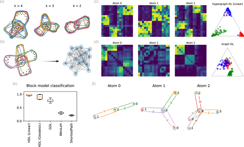
Figure 9: (a) Sample instances from the hypergraph block model for $k=4,3,2$ blocks. (b) Illustration of hypergraph flattening. (c) (i) Learned hypergraph atoms capture the three underlying block models. Note the presence of hyperedges that span the vertex set between blocks. (ii) Barycentric projection of learned weights, colored by the ground truth label. (d) Learned graph atoms (i) and weights (ii) from Gromov-Wasserstein dictionary learning with flattened hypergraphs as input. (e) 10-fold cross-validation results for SVM classification of hypergraph block-model samples. (f) Coarse-grained hypergraph representations of dictionary atoms learned by linear HDL.

5.5.4 Example: mutagenicity dataset

A real-world example is the well known MUTAG dataset [22] of 188 small molecule structures, labeled by their mutagenicity (mutagenic or non-mutagenic). This is a standard benchmarking dataset that has been widely adopted for testing graph learning algorithms [52], where typically nodes are taken to be atoms, and edges are chemical bonds. Starting from the molecular graph where nodes are atoms and edges are bonds, we propose to lift these chemical structures to partitioned networks as follows. Using a graph heat kernel [19], we construct an atom-atom connectivity network encoding proximity of atoms in the molecule. We also construct a persistent homology (PH) hypergraph following the procedure described in [3] to encode information about geometric cycles: vertices and hyperedges correspond to atoms and PH generators, respectively. We show the ensemble of persistence diagrams from this dataset in Figure 10(a), where points are colored by the ground truth mutagenicity label. A separation between mutagenic and non-mutagenic compounds can be visually discerned from these persistence diagrams, suggesting that persistent homology may be sensitive to molecular features that play a role in mutagenicity. In Figure 10(b) we illustrate the computation of the connectivity kernel and the PH-hypergraph from an example molecular graph.

Taking either the PH-hypergraphs or (heat kernel, PH)-partitioned networks as input data, we run linearized partitioned network dictionary learning for $k=8$ atoms and extract the learned atoms and coefficients. We reason that the learned dictionaries should capture aspects of the molecular structure that are predictive of molecular properties such as mutagenicity. Using the learned coefficients, we train a RBF-kernel support vector machine for binary classification of mutagenicity. We also apply the linear Gromov-Wasserstein dictionary learning algorithm of [65] using the clique expansion of the PH-hypergraph as input. For reference, we consider several other popular approaches for encoding geometric and topological information in machine learning tasks. Specifically, we compare to persistence images [1] (PersImg), as well as the Weisfeiler-Lehmann graph kernel [51] using either the molecular connectivity graphs (WL-conn) or clique-expansion of PH-hypergraph (WL-ph).

We find (see Figure 10(c)) that both hypergraph and partitioned network dictionary learning achieved comparable performance, suggesting that information on PH generators alone is sufficient to distinguish between mutagenic and non-mutagenic compounds in the majority of cases. On the other hand, Gromov-Wasserstein dictionary learning exhibits worse performance despite being provided with PH information in the form of the clique-expansion of the PH hypergraph. This reflects the loss of higher-order information incurred by “flattening” of the hypergraph to a graph [53]. Similarly, we find that classification using persistence images (encoding information about the persistence diagram, but not vertex-generator membership information) as well as Weisfeiler-Lehman kernels (encoding only pairwise relationships) perform relatively poorly. In order to ensure a fair comparison across the different methods we consider, we do not use node labels in this analysis. We remark that our dictionary learning algorithm can be straightforwardly extended to incorporate vector-valued node labels [65] and we expect that including that additional information would further improve classification performance.

Figures 10(d, e) shows the atoms found by hypergraph and partitioned network dictionary learning, respectively. The learned atoms of the partitioned network dictionary consist of pairwise vertex-vertex similarities, as well as vertex-hyperedge memberships. The partitioned network atoms capture both local detail as well as topological information in a coupled fashion. By comparison, with only hypergraph information, vertices with membership in the same homology generators may be indistinguishable. The dictionary coefficients in Figure 10(f), illustrate how each molecule in the dataset is decomposed in terms of soft membership to each of the $k=8$ archetypes. From visual inspection, it is already clear that the learned topics are largely able to disentangle mutagenic compounds from non-mutagenic ones. To quantify this, we train a linear SVM on the hypergraph dictionary coefficients, and extract the contribution of each atom towards the “mutagenic” class (Figure 10(g)). We find that atoms are clearly separated into mutagenicity and non-mutagenicity contributing factors. In Figure 10(h) we show example PH-hypergraph archetypes that are indicative of (non-)mutagenicity. For instance Atom 0, which contributes towards non-mutagenicity, displays a simple PH-hypergraph structure with two generators that do not share vertices. On the other hand, Atom 4 contributes towards mutagenicity and displays a complex PH-hypergraph structure with many interlinked generators. These findings suggest that compounds with more cycles are more likely to be mutagenic, and this is consistent with the chemical literature [22].

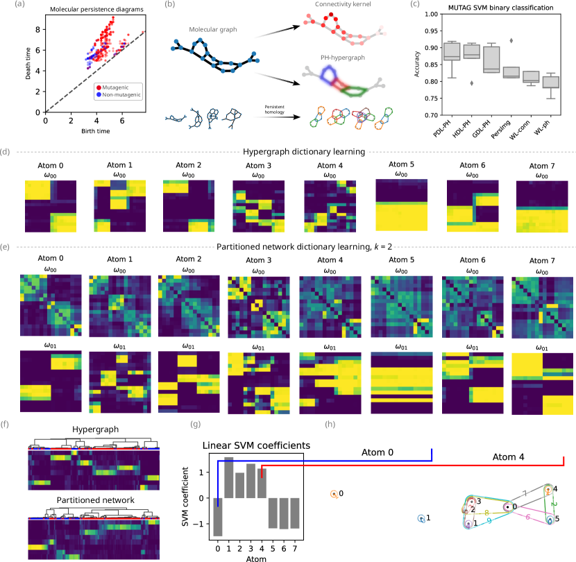
Figure 10: (a) Superimposed persistence diagrams ($H_{1}$, 1-dimensional persistent homology) for molecular structures in the MUTAG dataset, colored by mutagenicity. (b) Illustration of connectivity kernel and persistent homology (PH) hypergraph construction from molecular graphs. (c) SVM binary classification accuracy for mutagenicity, using different representations or kernels, shown over 5-fold cross validation. (d) Atoms learned by hypergraph dictionary learning (HDL). (e) Atoms learned by partitioned network dictionary learning (PDL). (f) Dictionary weights learned from hypergraph dictionary learning and partitioned network dictionary learning, respectively. (g) Coefficients learned from HDL weights by linear SVM. (h) Atom 0 (predicted to be associated with non-mutagenic compounds) and Atom 4 (predicted to be associated with mutagenic compounds).

6 Discussion

We develop a theoretical footing for analysis of generalized network objects, modeled by the space of $k$-partitioned measure networks. We equip this space with a family of metrics $d_{\mathcal{P}^{p}_{k}}$, $p\geq 1$ that extends the well-known $p$-Gromov-Wasserstein metric originally developed for measure metric spaces [55, 36] and recently applied to measure networks [17] and hypernetworks [20]. When $p=2$, we further provide a geometric characterization of this space in terms of geodesics, curvature bounds, as well as its tangent space. We additionally consider the case where additional labels, valued in a metric space, are available. We prove metric properties in this setting, and for $p=2$ we show that our geometric characterizations also apply, when labels are valued in an inner product space. Based on these ideas, we provide a range of numerical examples illustrating the applicability of our framework across several domains in network analysis and data science. We believe our work will be of broad interest to the network science, geometry and statistics communities.

Our work leaves several open avenues for future research. Among these, providing a geometric characterization (for instance, conditions for uniqueness of geodesics and curvature) of labeled networks when labels are valued in more general spaces, such as Riemannian manifolds. Additionally, a rigorous analysis of functionals on the space of partitioned measure networks and their gradient flows remains to be constructed. While we have introduced notions of tangent vectors and gradients and have formally shown their calculation and application, we did not address issues such as existence and uniqueness of minimizers in the general case.

On the applications front, some of the example applications we have presented could be fruitful problems to study separately. Among these, we think that multiscale network alignment and partitioned network dictionary learning are particularly interesting. As an example of a specific application requiring extensions of our theory, in [71] we develop a partial transport variant for applications in topological data analysis. Finally we remark that there are some alternative formulations of optimal transport applied to tensors [30] that our framework does not cover - whether similar theoretical results to ours can be established for this setting remains an open question.

Appendix A Numerical algorithms

A.1 Co-optimal transport

By taking $k=2$, $\omega_{ii}=0$, $\omega_{ij}=\omega_{ji}$, and noting that $\langle L(\omega,\omega^{\prime}),\pi\otimes\xi\rangle=\langle L(\omega^{\top},{\omega^{\prime}}^{\top}),\xi\otimes\pi\rangle$ we obtain from (32) the case of matching between labeled measure hypernetworks:

$$\min_{\begin{subarray}{c}\pi_{1}\in\Pi(\mu_{1},\mu_{1}^{\prime}),\pi_{2}\in\Pi(\mu_{2},\mu_{2}^{\prime})\end{subarray}}\langle L(\omega_{12},\omega^{\prime}_{12}),\pi_{1}\otimes\pi_{2}\rangle+\langle C_{1},\pi_{1}\rangle+\langle C_{2},\pi_{2}\rangle+\varepsilon_{1}\Omega_{1}(\pi_{1})+\varepsilon_{2}\Omega_{2}(\pi_{2}),$$ (43)

where for full generality we include the possibility of a regularization of the $\pi_{i}$ when $\varepsilon_{i}>0$, as per (33).

The unregularized problem is a bilinear program in $(\pi_{1},\pi_{2})$ since the objective can be rewritten $\langle L(\omega_{12},\omega_{12}^{\prime})+C_{1}\oplus C_{2},\pi_{1}\otimes\pi_{2}\rangle$ where $(A\oplus B)_{ijkl}=A_{ij}+B_{kl}$. In the case of unlabeled measure hypernetworks where $C_{1}=C_{2}=0$, this has been studied in detail by [59, 20]. The alternating scheme of [59] for finding a stationary point presents itself:

$$\begin{split}\pi_{1}\leftarrow\min_{\pi_{1}\in\Pi(\mu_{1},\mu_{1}^{\prime})}\langle&L(\omega_{12},\omega_{12}^{\prime})\otimes\pi_{2}+C_{1},\pi_{1}\rangle+\varepsilon_{1}\Omega_{1}(\pi_{1}),\\ \pi_{2}\leftarrow\min_{\pi_{2}\in\Pi(\mu_{2},\mu_{2}^{\prime})}\langle&L(\omega_{21},\omega_{21}^{\prime})\otimes\pi_{1}+C_{2},\pi_{2}\rangle+\varepsilon_{2}\Omega_{2}(\pi_{2}),\end{split}$$ (44)

Employing the identity [43, Proposition 1] we have for $\pi\in\Pi(\mu,\mu^{\prime})$ that

$$L(\omega,\omega^{\prime})\otimes\pi=\sum_{kl}L(\omega,\omega^{\prime})_{\cdot\cdot kl}\otimes\pi_{kl}=\eta(\omega,\omega^{\prime})-\omega\pi({\omega^{\prime}})^{\top},$$ (45)

where

$$\eta(\omega,\omega^{\prime})=\frac{1}{2}\left(\omega^{2}\right)\mu\mathbf{1}^{\top}+\frac{1}{2}\mathbf{1}\left({\omega^{\prime}}^{2}\mu^{\prime}\right)^{\top},$$ (46)

and $\omega^{2},{\omega^{\prime}}^{2}$ are understood entrywise. $\eta(\omega,\omega^{\prime})$ depends only upon $(\mu,\mu^{\prime})$, the marginals of $\pi$. Furthermore, we have the identity

$$\langle L(\omega_{12},\omega_{12}^{\prime}),\pi_{1}\otimes\pi_{2}\rangle=\langle L(\omega_{12},\omega_{12}^{\prime})\otimes\pi_{2},\pi_{1}\rangle=\langle L(\omega_{12}^{\top},(\omega_{12}^{\prime})^{\top})\otimes\pi_{1},\pi_{2}\rangle.$$

Algorithm 1 Alternating minimization: labeled hypergraphs (co-optimal transport)

1:Input: Incidence matrices $\omega_{12},\omega_{12}^{\prime}$, probability measures $\mu_{i},\mu_{i}^{\prime}$, $i=1,2$.

2:Initialize couplings: $\pi_{i}\leftarrow\mu_{i}\otimes\mu_{i}^{\prime},\>i=1,2.$

3:for $t=1,2,\dots,\texttt{max\_iter}$ do

4:     

$$\pi_{1}\leftarrow\operatorname*{arg\,min}_{\pi_{1}\in\Pi(\mu_{1},\mu_{1}^{\prime})}\langle L(\omega_{12},\omega_{12}^{\prime})\otimes\pi_{2}+C_{1},\pi_{1}\rangle+\varepsilon_{1}\Omega_{1}(\pi_{1}),$$

5:     

$$\pi_{2}\leftarrow\operatorname*{arg\,min}_{\pi_{2}\in\Pi(\mu_{2},\mu_{2}^{\prime})}\langle L(\omega_{21},\omega_{21}^{\prime})\otimes\pi_{1}+C_{2},\pi_{2}\rangle+\varepsilon_{2}\Omega_{2}(\pi_{2}),$$

6:end for

7:Output: couplings $(\pi_{1},\pi_{2})$

A.2 General matchings of partitioned measure networks

For general $k$-partitioned measure networks, the problem (32) is quadratic in pairs of $(\pi_{i},\pi_{j}),1\leq i,j\leq k$. This problem can be solved by a block coordinate descent separately in each of the $\pi_{i}$, where each block update amounts to solution of a problem closely resembling Fused Gromov-Wasserstein matching [61]. The update subproblem in each $\pi_{i}$ is therefore

$$\min_{\pi_{i}\in\Pi(\mu_{i},\mu_{i}^{\prime})}\frac{1}{2}\langle L(\omega_{ii},\omega^{\prime}_{ii}),\pi_{i}\otimes\pi_{i}\rangle+\langle M[\pi_{-i}]+C_{i},\pi_{i}\rangle+\varepsilon_{i}\Omega_{i}(\pi_{i}),\quad 1\leq i\leq k,$$ (47)

where $\pi_{-i}=\{\pi_{j},j\neq i\}$ and

$$\begin{split}M[\pi_{-i}]&=\sum_{j\neq i}\left(\frac{1}{2}L(\omega_{ij},\omega_{ij}^{\prime})+\frac{1}{2}L(\omega_{ji}^{\top},\omega_{ji}^{\prime\top})\right)\otimes\pi_{j}\\ &=\frac{1}{2}\sum_{j\neq i}\left[\eta(\omega_{ij},\omega^{\prime}_{ij})-\omega_{ij}\pi_{j}({\omega^{\prime}}_{ij})^{\top}+\eta(\omega_{ji}^{\top},{\omega^{\prime}}_{ji}^{\top})-\omega_{ji}^{\top}\pi_{j}\omega^{\prime}_{ji}\right],\end{split}$$ (48)

Each subproblem in $\pi_{i}$ amounts to minimization of a non-convex quadratic objective on a closed convex domain, and so a stationary point can be found using the conditional gradient algorithm of [61, Algorithm 1].

Algorithm 2 Alternating minimization: labeled $k$-partitioned networks

1:Input: Matrices $\{\omega_{ij}\}_{i,j=1}^{k},\{\omega_{ij}^{\prime}\}_{i,j=1}^{k}$, probability measures $\mu_{i},\mu_{i}^{\prime}$, $1\leq i\leq k$.

2:Initialize couplings: $\pi_{i}\leftarrow\mu_{i}\otimes\mu_{i}^{\prime},\>1\leq i\leq k.$

3:for $t=1,2,\dots,\texttt{max\_iter}$ do

4:     for $1\leq i\leq k$ do

5:         

$$\pi_{i}\leftarrow\operatorname*{arg\,min}_{\pi_{i}\in\Pi(\mu_{i},\mu_{i}^{\prime})}\frac{1}{2}\langle L(\omega_{ii},\omega^{\prime}_{ii}),\pi_{i}\otimes\pi_{i}\rangle+\langle M[\pi_{-i}]+C_{i},\pi_{i}\rangle+\varepsilon_{i}\Omega_{i}(\pi_{i}),$$

6:     end for

7:end for

8:Output: couplings $\{\pi_{i}\}_{i=1}^{k}$

A.3 Proximal gradient methods

As an alternative to relying on network simplex solvers for the unregularized problem, an entropic proximal gradient algorithm can also be used to solve the problem (32). These algorithms have been shown to perform favorably in terms of computational complexity as well as empirical results [69, 66]. Writing

$$\mathsf{L}(\pi_{1},\ldots,\pi_{k})=\frac{1}{2}\sum_{i,j=1}^{k}\langle L(\omega_{ij},\omega_{ij}^{\prime}),\pi_{i}\otimes\pi_{j}\rangle+\sum_{i=1}^{k}\langle C_{i},\pi_{i}\rangle.$$ (49)

to be the objective function of (32) and choosing a regularization level (inverse step size schedule) $\lambda^{t}>0$, a proximal gradient descent on the objective $\mathsf{L}$ starting from an initialization $(\pi_{i}^{0})$ generates the iterates for $t\geq 0$:

$$(\pi_{i}^{t+1})_{i=1}^{k}\leftarrow\operatorname*{arg\,min}_{\pi_{i}\in\Pi(\mu_{i},\mu_{i}^{\prime}),\>1\leq i\leq k}\mathsf{L}(\pi_{1},\ldots,\pi_{k})+\lambda^{t}\operatorname{KL}(\otimes_{i}\pi_{i}|\otimes_{i}\pi_{i}^{t}),$$ (50)

where $\operatorname{KL}(\alpha|\beta)$ denotes the (generalized) Kullback-Leibler divergence between probability distributions (positive measures)

$$\operatorname{KL}(\alpha|\beta)=\langle\alpha,\log(\mathrm{d}\alpha/\mathrm{d}\beta)\rangle-|\alpha|+|\beta|.$$

Replacing $\mathsf{L}$ with its linearization about $(\pi_{1}^{t},\ldots,\pi_{k}^{t})$ yields the proximal gradient method [40],

$$(\pi_{i}^{t+1})_{i=1}^{k}\leftarrow\operatorname*{arg\,min}_{\pi_{i}\in\Pi(\mu_{i},\mu_{i}^{\prime}),1\leq i\leq k}\sum_{i=1}^{k}\langle\nabla_{i}\mathsf{L}(\pi_{1}^{t},\ldots,\pi_{k}^{t}),\pi_{i}\rangle+\lambda^{t}\operatorname{KL}(\otimes_{i}\pi_{i}|\otimes_{i}\pi_{i}^{t}),$$ (51)

where $\nabla_{i}$ denotes the gradient of $\mathsf{L}$ in its $i$th argument. Since (for all probability measure inputs) $\operatorname{KL}(\otimes_{i}\pi_{i}|\otimes_{i}\pi_{i}^{t})=\sum_{i}\operatorname{KL}(\pi_{i}|\pi_{i}^{t})$, the proximal gradient update decouples in each of the $\pi_{i}$:

$$\pi_{i}^{t+1}\leftarrow\operatorname*{arg\,min}_{\pi_{i}\in\Pi(\mu_{i},\mu_{i}^{\prime})}\langle\nabla_{i}\mathsf{L}(\pi_{1}^{t},\ldots,\pi_{k}^{t}),\pi_{i}\rangle+\lambda^{t}\operatorname{KL}(\pi_{i}|\pi_{i}^{t}),\quad 1\leq i\leq k.$$ (52)

Rewriting each problem leads to an entropic optimal transport problem which can be solved via Sinkhorn iterations [21]:

$$\begin{split}&\pi_{i}^{t+1}\leftarrow\operatorname*{arg\,min}_{\pi_{i}\in\Pi(\mu_{i},\mu_{i}^{\prime})}\lambda^{t}\operatorname{KL}(\pi_{i}|\pi_{i}^{t}\odot e^{-M_{i}/\lambda^{t}}),\quad M_{i}=\nabla_{i}\mathsf{L}(\pi_{1}^{t},\ldots,\pi_{i}^{t}),\quad 1\leq i\leq k.\end{split}$$ (53)

Noting that

$$\frac{\partial}{\partial\pi}\frac{1}{2}\langle L(\omega,\omega^{\prime}),\pi\otimes\pi\rangle=\left(\frac{1}{2}L(\omega,\omega^{\prime})+\frac{1}{2}L(\omega^{\top},{\omega^{\prime}}^{\top})\right)\otimes\pi,$$

we have the following formula for $\nabla_{i}\mathsf{L}$:

$$\nabla_{i}\mathsf{L}(\pi_{1},\ldots,\pi_{k}) =\frac{1}{2}\left(L(\omega_{ii},\omega^{\prime}_{ii})+L(\omega_{ii}^{\top},{\omega^{\prime}}_{ii}^{\top})\right)\otimes\pi_{i}+M[\pi_{-i}]+C_{0}$$

where $M[\pi_{-i}]$ is defined in (48).

Algorithm 3 Proximal gradient: labeled $k$-partitioned networks

1:Input: Matrices $\{\omega_{ij}\}_{i,j=1}^{k},\{\omega_{ij}^{\prime}\}_{i,j=1}^{k}$, probability measures $\mu_{i},\mu_{i}^{\prime}$, $1\leq i\leq k$.

2:Initialize couplings: $\pi_{i}^{1}\leftarrow\mu_{i}\otimes\mu_{i}^{\prime},\>1\leq i\leq k.$

3:for $t=1,2,\dots,\texttt{max\_iter}$ do

4:     for $1\leq i\leq k$ do

5:         $M_{i}\leftarrow\frac{1}{2}\left(L(\omega_{ii},\omega^{\prime}_{ii})+L(\omega_{ii}^{\top},{\omega^{\prime}}_{ii}^{\top})\right)\otimes\pi_{i}^{t}+M[\pi_{-i}^{t}]+C_{0}$  (see Eq. (48))

6:         $\pi_{i}^{t+1}\leftarrow\operatorname*{arg\,min}_{\pi_{i}\in\Pi(\mu_{i},\mu_{i}^{\prime})}\lambda^{t}\operatorname{KL}(\pi_{i}|\pi_{i}^{t}\odot e^{-M_{i}/\lambda^{t}})$  (solve using Sinkhorn algorithm).

7:     end for

8:end for

9:Output: couplings $\{\pi_{i}\}_{i=1}^{k}$

We remark that when all the $\omega_{ii}=0$, then $\mathsf{L}$ coincides with its linearization and Algorithm 3 is in fact a proximal point method.

Proposition 54 (Convergence of proximal point method).

The limiting iterates as $t\to\infty$ of the problem (50) converge to a stationary point of (32).

Proof.

Writing $\pi=(\pi_{1},\ldots,\pi_{k})$, (50) can be written as

$$\min_{\pi\in U}u(\pi,\pi^{t}),$$

where

$$u(\pi,\pi^{\prime})=\mathsf{L}(\pi_{1},\ldots,\pi_{k})+\lambda\operatorname{KL}(\otimes_{i}\pi_{i}|\otimes_{i}\pi_{i}^{\prime})$$

and the set $U=\times_{i=1}^{k}\Pi(\mu_{i},\mu_{i}^{\prime})$ is closed and convex as a Cartesian product of closed, convex sets. Now we note that

• $u(\pi,\pi)=\mathsf{L}(\pi)$ for all $\pi\in U$.

• $u(\pi,\pi^{\prime})\geq\mathsf{L}(\pi)$ by non-negativity of the $\operatorname{KL}$-divergence

• $u(\pi,\pi^{\prime})$ is smooth in both of its arguments.

Taken together and applying [45, Proposition 1], we satisfy the conditions for [45, Theorem 1].

We remark that the unbalanced case (where the hard marginal constraints are replaced by soft constraints) can be handled in the same way, if the marginal penalties are smooth. The constraint set is then $U=\times_{i=1}^{k}\mathcal{M}_{+}$ which is also closed and convex. ∎

A.4 Projected gradient descent

When a solution to the regularized problem (33) is sought and $\Omega_{0}=\Omega_{1}=\operatorname{KL}$, a projected gradient descent approach [43] can be used. Then the minimization problem has the form

$$\min_{\pi_{i}\in\Pi(\mu_{i},\mu_{i}^{\prime}),1\leq i\leq k}\mathsf{L}(\pi_{1},\ldots,\pi_{k})+\sum_{i=1}^{k}\varepsilon_{i}\operatorname{KL}(\pi_{i}|\mu_{i}\otimes\mu_{i}^{\prime}).$$ (54)

For a gradient step size $\eta_{i}>0$, a projected mirror descent step in each $\pi_{i}$ reads

$$\pi_{i}^{t+1}\leftarrow\operatorname{Proj}_{\Pi(\mu_{i},\mu_{i}^{\prime})}^{\operatorname{KL}}\left[\pi_{i}^{t}\odot\exp\left(-\eta(\nabla_{i}\mathsf{L}(\pi_{1}^{t},\ldots,\pi_{k}^{t})+\varepsilon_{i}\log(\pi_{i}^{t}/\mu_{i}\otimes\mu_{i}^{\prime}))\right)\right],\quad 1\leq i\leq k.$$ (55)

Choosing $\eta_{i}=1/\varepsilon_{i}$, we get

$$\pi_{i}^{t+1}\leftarrow\operatorname{Proj}_{\Pi(\mu_{i},\mu_{i}^{\prime})}^{\operatorname{KL}}\left[e^{-\varepsilon_{i}^{-1}\nabla_{i}\mathsf{L}(\pi_{1},\ldots,\pi_{k})}\mu_{i}\otimes\mu_{i}^{\prime}\right],\quad 1\leq i\leq k.$$ (56)

Each of these projections can be computed through the Sinkhorn algorithm [43, 21]. Similarly, one may consider $\Omega_{i}=\frac{1}{2}\|\cdot\|_{L^{2}(\mu_{i}\otimes\mu^{\prime}_{i})}^{2}$, in which case the projected $L^{2}$-gradient descent steps are

$$\pi^{t+1}_{i}\leftarrow\operatorname{Proj}_{\Pi(\mu_{i},\mu_{i}^{\prime})}^{F}\left[-\frac{1}{\varepsilon_{i}}\nabla_{i}\mathsf{L}(\pi_{1}^{t},\ldots,\pi_{k}^{t})(\mu_{i}\otimes\mu_{i}^{\prime})\right],\quad 1\leq i\leq k,$$ (57)

where here both the gradient and projection steps are calculated in $L^{2}(\mu\otimes\mu^{\prime})$. The $L^{2}$-projection $\operatorname{Proj}_{\Pi(\mu,\mu^{\prime})}^{F}(A)$ can be carried out by solving a quadratically regularized optimal transport problem. This formulation has the notable advantage of producing couplings which are sparse, i.e. identically zero outside of a support set.

Algorithm 4 Projected gradient: labeled $k$-partitioned networks, regularized matchings

1:Input: Matrices $\{\omega_{ij}\}_{i,j=1}^{k},\{\omega_{ij}^{\prime}\}_{i,j=1}^{k}$, probability measures $\mu_{i},\mu_{i}^{\prime}$, $1\leq i\leq k$.

2:Initialize couplings: $\pi_{i}^{1}\leftarrow\mu_{i}\otimes\mu_{i}^{\prime},\>1\leq i\leq k.$

3:for $t=1,2,\dots,\texttt{max\_iter}$ do

4:     for $1\leq i\leq k$ do

5:         $M_{i}\leftarrow\frac{1}{2}\left(L(\omega_{ii},\omega^{\prime}_{ii})+L(\omega_{ii}^{\top},{\omega^{\prime}}_{ii}^{\top})\right)\otimes\pi_{i}^{t}+M[\pi_{-i}^{t}]+C_{0}$  (see Eq. (48))

6:         $\pi_{i}^{t+1}\leftarrow\operatorname*{arg\,min}_{\pi_{i}\in\Pi(\mu_{i},\mu_{i}^{\prime})}\varepsilon_{i}\operatorname{KL}(\pi_{i}|e^{-\varepsilon_{i}^{-1}M_{i}}\mu_{i}\otimes\mu_{i}^{\prime})$

7:     end for

8:end for

9:Output: couplings $\{\pi_{i}\}_{i=1}^{k}$

A.5 Unbalanced matchings

We now consider the setting of unbalanced transport, in which marginal constraints are relaxed and replaced with penalty functions that enforce a “soft” marginal constraint. Unbalanced transport has been well studied from both a theoretical and practical viewpoint for the transportation of measures [14, 13, 34], and has since been extended to the setting of (fused) Gromov-Wasserstein matchings between metric measure spaces [49, 57] and co-optimal transport [60]. An unbalanced formulation of the partitioned network alignment problem is valuable in practical settings when there may only be partial correspondences between networks, such as in the metabolic network alignment example of Figure 3.

The unbalanced transport problem for labeled partitioned measure networks includes unbalanced (fused) Gromov-Wasserstein and co-optimal transport as sub-cases. We let $\lambda_{1,2}>0$ enforce the soft marginal constraints for the source and target respectively, and we denote by $\mathcal{M}_{+}(X)$ the space of positive measures supported on $X$. For generality, and because this makes efficient computational schemes possible, we optionally allow an entropic regularization with coefficient $\varepsilon\geq 0$. Then we pose the problem of (entropically regularized) unbalanced matching as

$$\begin{split}\min_{\begin{subarray}{c}\pi_{i}\in\mathcal{M}_{+}(X_{i}\times X_{i}^{\prime}),\>1\leq i\leq k,\\ m(\pi_{i})=m(\pi_{j}),\>\forall 1\leq i,j\leq k\end{subarray}}\>\widetilde{\mathsf{L}}(\pi_{1},\ldots,\pi_{k})&+\varepsilon\sum_{i,j=1}^{k}\operatorname{KL}(\pi_{i}\otimes\pi_{j}|\mu_{i}\otimes\mu_{i}^{\prime}\otimes\mu_{j}\otimes\mu_{j}^{\prime})\\ &+\lambda_{1}\sum_{i,j=1}^{k}\operatorname{KL}(\pi_{i}\mathbf{1}\otimes\pi_{j}\mathbf{1}|\mu_{i}\otimes\mu_{j})+\lambda_{2}\sum_{i,j=1}^{k}\operatorname{KL}(\pi_{i}^{\top}\mathbf{1}\otimes\pi_{j}^{\top}\mathbf{1}|\mu_{i}^{\prime}\otimes\mu_{j}^{\prime}).\end{split}$$ (58)

In the above, $\widetilde{\mathsf{L}}$ denotes a variant of the objective function (49), modified to ensure that the function to be minimized remains homogeneous in $(\pi_{1},\ldots,\pi_{k})$:

$$\widetilde{\mathsf{L}}(\pi_{1},\ldots,\pi_{k})=\frac{1}{2}\sum_{i,j=1}^{k}\langle L(\omega_{ij},\omega^{\prime}_{ij}),\pi_{i}\otimes\pi_{j}\rangle+\sum_{i=1}^{k}m(\pi_{i})\langle C_{i},\pi_{i}\rangle.$$ (59)

This is different to the setup in [57], in which the quadratic nature of the Gromov-Wasserstein term in the coupling $\pi$ conflicts with the linearity of the fused term. Importantly, $\widetilde{\mathsf{L}}$ coincides with $\mathsf{L}$ when its inputs are restricted to be probability measures, i.e. $m(\pi_{i})=1$.

Extending the definition of partitioned measure networks (Definition 7), we will allow $\mu_{i}$ to be positive measures in $\mathcal{M}_{+}(X_{i})$ for each $1\leq i\leq k$, but require that $m(\mu_{i})=m(\mu_{j}),i\neq j$. The motivation for doing so is to eliminate the non-uniqueness under scalings e.g. $(\mu_{i},\mu_{j})\to(\lambda\mu_{i},\lambda^{-1}\mu_{j})$ that becomes a particular issue in the special case of co-optimal transport [60].

First, we state the identity

$$\operatorname{KL}(\alpha\otimes\beta|\alpha^{\prime}\otimes\beta^{\prime}) =m(\beta)\operatorname{H}(\alpha|\alpha^{\prime})+m(\alpha)\operatorname{H}(\beta|\beta^{\prime})-m(\alpha)m(\beta)+m(\alpha^{\prime})m(\beta^{\prime})$$

$$=m(\beta)\operatorname{KL}(\alpha|\alpha^{\prime})+m(\alpha)\operatorname{KL}(\beta|\beta^{\prime})+(m(\alpha)-m(\alpha^{\prime}))(m(\beta)-m(\beta^{\prime})),$$

where we have defined the relative entropy term

$$\operatorname{H}(\alpha|\alpha^{\prime})=\int\log\left(\frac{\mathrm{d}\alpha}{\mathrm{d}\alpha^{\prime}}\right)\mathrm{d}\alpha.$$

Thus, $(\alpha,\beta)\mapsto\operatorname{KL}(\alpha\otimes\beta|\alpha^{\prime}\otimes\beta^{\prime})$ is 2-homogeneous up to additive constants [49]. Since $\widetilde{\mathsf{L}}$ is 2-homogeneous, the objective of (58) is also 2-homogeneous. We remark that this is important, since if we used $\mathsf{L}$ instead of $\widetilde{\mathsf{L}}$, under the scaling $\pi_{i}\mapsto\lambda\pi_{i}$ quadratic terms would dominate when $\lambda\to+\infty$ and linear terms when $\lambda\to 0$.

Special case: measure hypernetworks

A special case is when $k=2$ and $\omega_{ii}=\omega^{\prime}_{ii}=0$: this amounts to an unbalanced, fused co-optimal transport problem. This was the focus of [60] which considered the unlabeled setting, and we discuss it for completeness. In this case, $\widetilde{\mathsf{L}}$ can be written in a bilinear form in $(\pi_{1},\pi_{2})$:

$$\widetilde{\mathsf{L}}(\pi_{1},\pi_{2})=\left\langle\frac{1}{2}L(\omega_{12},\omega_{12}^{\prime})+\frac{1}{2}L(\omega_{21}^{\top},\omega_{21}^{\prime\top})+C_{1}\otimes\mathbf{1}+\mathbf{1}\otimes C_{2},\pi_{1}\otimes\pi_{2}\right\rangle.$$

Up to additive constants, the problem (58) for $k=2$ and $\omega_{ii}=\omega^{\prime}_{ii}=0$ can be re-written as

$$\min_{\pi_{1},\pi_{2}}\widetilde{\mathsf{L}}(\pi_{1},\pi_{2}) +2\lambda_{1}\left((m(\pi_{1})+m(\pi_{2}))\operatorname{H}(\pi_{1}\mathbf{1}|\mu_{1})+(m(\pi_{1})+m(\pi_{2}))\operatorname{H}(\pi_{2}\mathbf{1}|\mu_{2})\right)$$

$$+2\lambda_{2}\left((m(\pi_{1})+m(\pi_{2}))\operatorname{H}(\pi_{1}^{\top}\mathbf{1}|\mu_{1}^{\prime})+(m(\pi_{1})+m(\pi_{2}))\operatorname{H}(\pi_{2}^{\top}\mathbf{1}|\mu_{2}^{\prime})\right)$$

$$+2\varepsilon\left((m(\pi_{1})+m(\pi_{2}))\operatorname{H}(\pi_{1}|\mu_{1}\otimes\mu_{1})+(m(\pi_{1})+m(\pi_{2}))\operatorname{H}(\pi_{2}|\mu_{2}\otimes\mu_{2}^{\prime}))\right)$$

$$-(\lambda_{1}+\lambda_{2}+\varepsilon)\left(m(\pi_{1})^{2}+m(\pi_{2})^{2}+2m(\pi_{1})m(\pi_{2})\right),$$

where the minimum is taken over $\pi_{1}\in\mathcal{M}_{+}(X_{1}\times X_{1}^{\prime})$ and $\pi_{2}\in\mathcal{M}_{+}(X_{2}\times X_{2})$ such that $m(\pi_{1})=m(\pi_{2})$. Notice that $\widetilde{\mathsf{L}}$ is bilinear, but the terms corresponding to the soft marginal constraints contain quadratic terms in $\pi_{1}$ and $\pi_{2}$. However, since we have the constraint $m(\pi_{1})=m(\pi_{2})$, we could judiciously swap $m(\pi_{1})$ and $m(\pi_{2})$ to derive an objective that remains equivalent under the mass equality constraint:

$$\min_{\pi_{1},\pi_{2}}\widetilde{\mathsf{L}}(\pi_{1},\pi_{2}) +4\lambda_{1}\left(m(\pi_{2})\operatorname{H}(\pi_{1}\mathbf{1}|\mu_{1})+m(\pi_{1})\operatorname{H}(\pi_{2}\mathbf{1}|\mu_{2})\right)$$

$$+4\lambda_{2}\left(m(\pi_{2})\operatorname{H}(\pi_{1}^{\top}\mathbf{1}|\mu_{1}^{\prime})+m(\pi_{1})\operatorname{H}(\pi_{2}^{\top}\mathbf{1}|\mu_{2}^{\prime})\right)$$

$$+4\varepsilon\left(m(\pi_{2})\operatorname{H}(\pi_{1}|\mu_{1}\otimes\mu_{1}^{\prime})+m(\pi_{1})\operatorname{H}(\pi_{2}|\mu_{2}\otimes\mu_{2}^{\prime})\right)$$

$$-4(\lambda_{1}+\lambda_{2}+\varepsilon)m(\pi_{1})m(\pi_{2}).$$

In what follows, we drop the factor of 4 as it can be absorbed into the coefficients:

$$\min_{\pi_{1},\pi_{2}}\widetilde{\mathsf{L}}(\pi_{1},\pi_{2}) +\lambda_{1}\left(m(\pi_{2})\operatorname{H}(\pi_{1}\mathbf{1}|\mu_{1})+m(\pi_{1})\operatorname{H}(\pi_{2}\mathbf{1}|\mu_{2})\right)$$

$$+\lambda_{2}\left(m(\pi_{2})\operatorname{H}(\pi_{1}^{\top}\mathbf{1}|\mu_{1}^{\prime})+m(\pi_{1})\operatorname{H}(\pi_{2}^{\top}\mathbf{1}|\mu_{2}^{\prime})\right)$$

$$+\varepsilon\left(m(\pi_{2})\operatorname{H}(\pi_{1}|\mu_{1}\otimes\mu_{1}^{\prime})+m(\pi_{1})\operatorname{H}(\pi_{2}|\mu_{2}\otimes\mu_{2}^{\prime})\right)$$

$$-(\lambda_{1}+\lambda_{2}+\varepsilon)m(\pi_{1})m(\pi_{2}).$$

We will for now remove the constraint $m(\pi_{1})=m(\pi_{2})$. In this setting, we can tackle the problem by alternating block minimization in $(\pi_{1},\pi_{2})$. Fixing $\pi_{2}$ and rearranging the objective function, the update in $\pi_{1}$ amounts to

$$\min_{\pi_{1}\in\mathcal{M}_{+}(X_{1}\times X_{1}^{\prime})}\langle M[\pi_{2}],\pi_{1}\rangle+\lambda_{1}m(\pi_{2})\operatorname{KL}(\pi_{1}\mathbf{1}|\mu_{1})+\lambda_{2}m(\pi_{2})\operatorname{KL}(\pi_{1}^{\top}\mathbf{1}|\mu_{1}^{\prime})+\varepsilon m(\pi_{2})\operatorname{KL}(\pi_{1}|\mu_{1}\otimes\mu_{1}^{\prime})$$ (60)

where

$$\begin{split}M[\pi_{2}]=&\left(\frac{1}{2}L(\omega_{12},\omega_{12}^{\prime})+\frac{1}{2}L(\omega_{21}^{\top},{\omega^{\prime}}_{21}^{\top})\right)\otimes\pi_{2}\\ &+m(\pi_{2})C_{1}+\left(\langle C_{2},\pi_{2}\rangle+\lambda_{1}\operatorname{H}(\pi_{2}\mathbf{1}|\mu_{2})+\lambda_{2}\operatorname{H}(\pi_{2}^{\top}\mathbf{1}|\mu_{2}^{\prime})+\varepsilon\operatorname{H}(\pi_{2}|\mu_{2}\otimes\mu_{2}^{\prime})\right)\mathbf{1}.\end{split}$$ (61)

Fixing $\pi_{1}$, the update in $\pi_{2}$ is

$$\min_{\pi_{2}\in\mathcal{M}_{+}(X_{2}\times X_{2}^{\prime})}\langle M[\pi_{1}],\pi_{2}\rangle+\lambda_{1}m(\pi_{1})\operatorname{KL}(\pi_{2}\mathbf{1}|\mu_{2})+\lambda_{2}m(\pi_{1})\operatorname{KL}(\pi_{2}^{\top}\mathbf{1}|\mu_{2}^{\prime})+\varepsilon m(\pi_{1})\operatorname{KL}(\pi_{2}|\mu_{2}\otimes\mu_{2}^{\prime})$$ (62)

where

$$\begin{split}M[\pi_{1}]=&\left(\frac{1}{2}L(\omega_{12}^{\top},{\omega^{\prime}}_{12}^{\top})+\frac{1}{2}L(\omega_{21},\omega^{\prime}_{21})\right)\otimes\pi_{1}\\ &+m(\pi_{1})C_{2}+\left(\langle C_{1},\pi_{1}\rangle+\lambda_{1}\operatorname{H}(\pi_{1}\mathbf{1}|\mu_{1})+\lambda_{2}\operatorname{H}(\pi_{1}^{\top}\mathbf{1}|\mu_{1}^{\prime})+\varepsilon\operatorname{H}(\pi_{1}|\mu_{1}\otimes\mu_{1}^{\prime})\right)\mathbf{1}.\end{split}$$ (63)

To enforce the equal mass constraint $m(\pi_{1})=m(\pi_{2})$, given $(\pi_{1},\pi_{2})$ with $m(\pi_{1})\neq m(\pi_{2})$, we use the following to project onto the constraint set:

$$(\pi_{1},\pi_{2})\mapsto\left(\sqrt{\frac{m(\pi_{2})}{m(\pi_{1})}}\pi_{1},\sqrt{\frac{m(\pi_{1})}{m(\pi_{2})}}\pi_{2}\right).$$

This projection, also used in [60], can be shown to be equivalent to the $\operatorname{KL}$-projection of $(\pi_{1},\pi_{2})$ onto the set $m(\pi_{1})=m(\pi_{2})$.

Algorithm 5 Unbalanced matchings: labeled measure hypernetworks

1:Input: Matrices $\omega_{12},\omega_{12}^{\prime}$, positive measures $\mu_{i},\mu_{i}^{\prime}$, $i=1,2$.

2:Initialize couplings: $\pi_{i}\leftarrow\mu_{i}\otimes\mu_{i}^{\prime}/\sqrt{m(\mu_{i})m(\mu_{i}^{\prime})},\>i=1,2.$

3:for $t=1,2,\dots,\texttt{max\_iter}$ do

4:     

$$\pi_{1}\leftarrow\operatorname*{arg\,min}_{\pi_{1}\in\mathcal{M}_{+}(X_{1}\times X_{1}^{\prime})}\langle M[\pi_{2}],\pi_{1}\rangle+\lambda_{1}m(\pi_{2})\operatorname{KL}(\pi_{1}\mathbf{1}|\mu_{1})+\lambda_{2}m(\pi_{2})\operatorname{KL}(\pi_{1}^{\top}\mathbf{1}|\mu_{1}^{\prime})+\varepsilon m(\pi_{2})\operatorname{KL}(\pi_{1}|\mu_{1}\otimes\mu_{1}^{\prime})$$

5:     $\pi_{1}\leftarrow\sqrt{\dfrac{m(\pi_{2})}{m(\pi_{1})}}\pi_{1}$

6:     

$$\pi_{2}\leftarrow\operatorname*{arg\,min}_{\pi_{2}\in\mathcal{M}_{+}(X_{2}\times X_{2}^{\prime})}\langle M[\pi_{1}],\pi_{2}\rangle+\lambda_{1}m(\pi_{1})\operatorname{KL}(\pi_{2}\mathbf{1}|\mu_{2})+\lambda_{2}m(\pi_{1})\operatorname{KL}(\pi_{2}^{\top}\mathbf{1}|\mu_{2}^{\prime})+\varepsilon m(\pi_{1})\operatorname{KL}(\pi_{2}|\mu_{2}\otimes\mu_{2}^{\prime})$$

7:     $\pi_{2}\leftarrow\sqrt{\dfrac{m(\pi_{1})}{m(\pi_{2})}}\pi_{2}$

8:end for

9:Output: couplings $\{\pi_{i}\}_{i=1}^{k}$

General case

For general partitioned measure networks, the objective function $\widetilde{\mathsf{L}}$ introduces terms that are non-trivially quadratic in $\pi_{i}$ and is therefore less straightforward to solve. While in the balanced case these kinds of problems are typically tackled using a Frank-Wolfe algorithm [36], such an approach is not feasible for problems with soft constraints. As done in related works [57, 49], we propose to solve the problem instead via a biconvex relaxation. Consider two partitioned couplings $(\pi_{1},\ldots,\pi_{k})$ and $(\xi_{1},\ldots,\xi_{k})$. We rewrite the equation (58):

$$\begin{split}\min_{\begin{subarray}{c}\pi_{i},\xi_{i}\in\mathcal{M}_{+}(X_{i}\times X_{i}^{\prime}),1\leq i\leq k\\ m(\pi_{i})=m(\xi_{j}),1\leq i,j\leq k\end{subarray}}\>&\widetilde{\mathsf{L}}(\pi_{1},\ldots,\pi_{k};\xi_{1},\ldots,\xi_{k})+\varepsilon\sum_{i,j=1}^{k}\operatorname{KL}(\pi_{i}\otimes\xi_{j}|\mu_{i}\otimes\mu_{i}^{\prime}\otimes\mu_{j}\otimes\mu_{j}^{\prime})\\ &+\lambda_{1}\sum_{i,j=1}^{k}\operatorname{KL}(\pi_{i}\mathbf{1}\otimes\xi_{j}\mathbf{1}|\mu_{i}\otimes\mu_{j})+\lambda_{2}\sum_{i,j=1}^{k}\operatorname{KL}(\pi_{i}^{\top}\mathbf{1}\otimes\xi_{j}^{\top}\mathbf{1}|\mu_{i}^{\prime}\otimes\mu_{j}^{\prime}),\end{split}$$ (64)

where we define the relaxed version of (59):

$$\widetilde{\mathsf{L}}(\pi_{1},\ldots,\pi_{k};\xi_{1},\ldots,\xi_{k}) =\frac{1}{2}\sum_{i,j=1}^{k}\langle L(\omega_{ij},\omega_{ij}^{\prime}),\pi_{i}\otimes\xi_{j}\rangle+\sum_{i=1}^{k}\left\langle\frac{1}{2}(C_{i}\otimes\mathbf{1}+\mathbf{1}\otimes C_{i}),\pi_{i}\otimes\xi_{i}\right\rangle.$$

This problem is now biconvex separately in $(\pi_{i})_{i=1}^{k}$ and $(\xi_{i})_{i=1}^{k}$. Fixing $(\xi_{i})_{i=1}^{k}$ and minimizing in $(\pi_{i})_{i=1}^{k}$, we find that the problem decouples across partitions:

$$\begin{split}\min_{\begin{subarray}{c}\pi_{i}\in\mathcal{M}_{+}(X_{i}\times X_{i}^{\prime}),1\leq i\leq k\\ m(\pi_{i})=m(\pi_{j}),1\leq i,j\leq k\end{subarray}}&\widetilde{\mathsf{L}}(\pi_{1},\ldots,\pi_{k};\xi_{1},\ldots,\xi_{k})\\ &+\left(\sum_{i}m(\pi_{i})\right)\left(\varepsilon\sum_{j}\operatorname{H}(\xi_{j}|\mu_{j}\otimes\mu_{j}^{\prime})+\lambda_{1}\sum_{j}\operatorname{H}(\xi_{j}\mathbf{1}|\mu_{j})+\lambda_{2}\sum_{j}\operatorname{H}(\xi_{j}^{\top}\mathbf{1}|\mu_{j}^{\prime})\right)\\ &+\lambda_{1}\left(\sum_{j}m(\xi_{j})\right)\sum_{i}\operatorname{KL}(\pi_{i}\mathbf{1}|\mu_{i})+\lambda_{2}\left(\sum_{j}m(\xi_{j})\right)\sum_{i}\operatorname{KL}(\pi_{i}^{\top}\mathbf{1}|\mu_{i}^{\prime})\\ &+\varepsilon\left(\sum_{j}m(\xi_{j})\right)\sum_{i}\operatorname{KL}(\pi_{i}|\mu_{i}\otimes\mu_{i}^{\prime}).\end{split}$$ (65)

Relaxing the mass equality constraint $m(\pi_{i})=m(\pi_{j}),1\leq i,j\leq k$, the above problem amounts to $k$ regularized unbalanced optimal transport problems that can be solved solved independently and in parallel. The resulting couplings can be projected onto the set $\{m(\pi_{i})=m(\pi_{j}),1\leq i,j\leq k\}$:

$$(\pi_{i})_{i=1}^{k}\mapsto\left(\frac{(m(\pi_{1})\ldots m(\pi_{k}))^{1/k}}{m(\pi_{i})}\pi_{i}\right)_{i=1}^{k}.$$ (66)

Similarly, fixing $(\pi_{i})_{i=1}^{k}$, the problem in $(\xi_{i})_{i=1}^{k}$ is

$$\begin{split}\min_{\begin{subarray}{c}\xi_{i}\in\mathcal{M}_{+}(X_{i}\times X_{i}^{\prime}),1\leq i\leq k\\ m(\xi_{i})=m(\xi_{j}),1\leq i,j\leq k\end{subarray}}&\widetilde{\mathsf{L}}(\pi_{1},\ldots,\pi_{k};\xi_{1},\ldots,\xi_{k})\\ &+\left(\sum_{j}m(\xi_{j})\right)\left(\varepsilon\sum_{i}\operatorname{H}(\pi_{i}|\mu_{i}\otimes\mu_{i}^{\prime})+\lambda_{1}\sum_{i}\operatorname{H}(\pi_{i}\mathbf{1}|\mu_{i})+\lambda_{2}\sum_{i}\operatorname{H}(\pi_{i}^{\top}\mathbf{1}|\mu_{i}^{\prime})\right)\\ &+\lambda_{1}\left(\sum_{i}m(\pi_{i})\right)\sum_{j}\operatorname{KL}(\xi_{j}\mathbf{1}|\mu_{j})+\lambda_{2}\left(\sum_{i}m(\pi_{i})\right)\sum_{j}\operatorname{KL}(\xi_{j}^{\top}\mathbf{1}|\mu_{j}^{\prime})\\ &+\varepsilon\left(\sum_{i}m(\pi_{i})\right)\sum_{j}\operatorname{KL}(\xi_{j}|\mu_{j}\otimes\mu_{j}^{\prime}),\end{split}$$ (67)

and the same projection (66) can be used to enforce the mass equality constraint in $(\xi_{i})_{i=1}^{k}$. It is important to note that this scheme aims to solve the biconvex relaxation (64) which is in general only a lower bound for (58). In particular, at convergence one may have $\pi_{i}\neq\xi_{i}$ in general. While this biconvex relaxation scheme was studied for the Gromov-Wasserstein setting by [49], they were unable to prove tightness or that the two sets of couplings $(\pi_{i})_{i},(\xi_{i})_{i}$ coincide.

Algorithm 6 Unbalanced matchings: labeled partitioned measure networks via biconvex relaxation

1:Input: Matrices $\{\omega_{ij}\}_{i,j=1}^{k},\{\omega_{ij}^{\prime}\}_{i,j=1}^{k}$, positive measures $\mu_{i},\mu_{i}^{\prime}$, $1\leq i\leq k$, marginal penalties $\lambda_{1},\lambda_{2}>0$, entropic regularization $\varepsilon\geq 0$.

2:Initialize couplings: $\pi_{i}\leftarrow\mu_{i}\otimes\mu_{i}^{\prime}/\sqrt{m(\mu_{i})m(\mu_{i}^{\prime})},\>1\leq i\leq k.$

3:Initialize additional couplings: $\xi_{i}\leftarrow\pi_{i},\>1\leq i\leq k.$

4:for $t=1,2,\dots,\texttt{max\_iter}$ do

5:     Update $(\pi_{1},\ldots,\pi_{k})$ by solving (65) independently for each $1\leq i\leq k$.

6:     Rescale $(\pi_{i})_{i=1}^{k}$ following (66)

7:     Update $(\xi_{1},\ldots,\xi_{k})$ by solving (67) independently for each $1\leq i\leq k$.

8:     Rescale $(\xi_{i})_{i=1}^{k}$ following (66)

9:     $(\pi_{i})_{i=1}^{k},(\xi_{i})_{i=1}^{k}\leftarrow\left(\sqrt{\frac{m(\xi)}{m(\pi)}}\pi_{i}\right)_{i=1}^{k},\left(\sqrt{\frac{m(\pi)}{m(\xi)}}\xi_{i}\right)_{i=1}^{k}$

10:end for

11:Output: couplings $\{\pi_{i}\}_{i=1}^{k},\{\xi_{i}\}_{i=1}^{k}$

A remark on partial transport

On the other hand we may consider partial transport, where some fraction $0\leq s\leq 1$ of mass is required to be transported with the remainder being discarded and thus incurring zero cost. This problem was considered by [12] in the case of Gromov-Wasserstein transport. For two probability measures $\mu,\mu^{\prime}$, define the set of partial couplings of mass $s$ to be

$$\Pi(\mu,\mu^{\prime};s)=\{\pi\geq 0:\pi\mathbf{1}\leq\mu,\pi^{\top}\mathbf{1}\leq\mu^{\prime},m(\pi)=s\}.$$

Then, the partial matching problem amounts to solving

$$\begin{split}\min_{\pi_{i}\in\Pi(\mu_{i},\mu_{i}^{\prime};s)}\mathsf{L}(\pi_{1},\ldots,\pi_{k}).\end{split}$$ (68)

This amounts to minimization of a non-convex objective on a convex and compact constraint set, and similar to [12] we can tackle it via conditional gradient method. In particular, for computation of the descent directions in each of the $\pi_{i}$ we need to solve:

$$\min_{\pi_{i}\in\Pi(\mu_{i},\mu_{i}^{\prime};s)}\langle\nabla_{i}\mathsf{L}(\pi_{1}^{t},\ldots,\pi_{k}^{t}),\pi_{i}\rangle.$$

Each of these is a partial optimal transport problem which can be solved using the virtual point approach of [12].

A.6 Partitioned networks for multiscale network matching

Chowdhury and Needham et al. [20] introduced a generalized co-optimal transport problem for multiscale network matching, where for an input graph $G$ successive topological simplifications $\mathcal{G}=\{G=G_{1},\ldots,G_{k}\}$ are produced. At each level $1\leq i\leq k-1$, the vertices of $G_{i}$ are partitioned among the vertices of $G_{i+1}$. In this way, the coupling of $G_{i}$ to $G_{i+1}$ can be modeled as a hypergraph in which vertices and hyperedges are identified with nodes in $G_{i}$ and $G_{i+1}$ respectively. We now show that $\mathcal{G}$ can be formulated as a partitioned network with $k$ partitions: let $X_{i}$ be the vertex set of the $i$th simplification level $G_{i}$. Let $\omega_{i,i+1}$ for $1\leq i\leq k-1$ be the function encoding relationships between vertices in the $i$th and vertices the $(i+1)$th simplification:

$$\omega(x,y)=\begin{cases}\omega_{i,i+1}(x,y),\quad&x\in X_{i},y\in X_{i+1}\text{ for }i=1,\ldots,k-1\\ \omega_{i+1,i}(x,y),\quad&x\in X_{i+1},y\in X_{i}\text{ for }i=1,\ldots,k-1\\ 0,\quad&\text{otherwise}.\end{cases}$$

Together with a choice of weights $(\mu_{i})_{i=1}^{k}$, $((X_{i},\mu_{i})_{i=1}^{k},\omega)$ is a partitioned measure network encoding the multiscale network $\mathcal{G}$.

Given two graphs $G,G^{\prime}$ and their simplifications $\mathcal{G},\mathcal{G}^{\prime}$, we can then construct two partitioned measure networks: $((X_{i},\mu_{i})_{i=1}^{k},\omega)$ and $((X_{i}^{\prime},\mu_{i}^{\prime})_{i=1}^{k},\omega^{\prime})$. For a candidate coupling $(\pi_{i})_{i=1}^{k}$, the corresponding distortion functional is

$$\sum_{i=1}^{k-1}\|\omega_{i,i+1}-\omega_{i,i+1}^{\prime}\|_{L^{p}(\pi_{i}\otimes\pi_{i+1})}^{p}.$$ (69)

The partitioned measure network alignment problem induced by this distortion is equivalent to the one proposed in [20, Algorithm 1], i.e.

$$\min_{\pi_{i}\in\Pi(\mu_{i},\mu_{i}^{\prime}),1\leq i\leq k}\sum_{i=1}^{k-1}\langle L(\omega_{i,i+1},\omega_{i,i+1}^{\prime}),\pi_{i}\otimes\pi_{i+1}\rangle.$$ (70)

This multiscale graph matching problem therefore fits into a generalized framework of partitioned measure networks. Encouragingly, while the formulation of [20] was in terms of pairs of couplings $(\pi_{i},\xi_{i}),1\leq i\leq k-1$ under the constraint $\xi_{i}=\pi_{i+1}$, the derivation of the problem from the viewpoint of partitioned measure networks allows us to directly and naturally formulate the problem in terms of a single set of couplings $(\pi_{1},\ldots,\pi_{k})$.

Furthermore, by modifying the function $\omega$ we can incorporate pairwise information on each of the graphs $G_{i}$:

$$\omega(x,y)=\begin{cases}\omega_{i,i+1}(x,y),\quad&x\in X_{i},y\in X_{i+1}\text{ for }i=1,\ldots,k-1\\ \omega_{i+1,i}(x,y),\quad&x\in X_{i+1},y\in X_{i}\text{ for }i=1,\ldots,k-1\\ \omega_{ii}(x,y),\quad&x,y\in X_{i}\times X_{i}\text{ for }i=1,\ldots,k\\ 0,\quad&\text{otherwise}.\end{cases}$$

This choice of $\omega$ leads to the problem

$$\min_{\pi_{i}\in\Pi(\mu_{i},\mu_{i}^{\prime})}\>\sum_{i=1}^{k-1}\langle L(\omega_{i,i+1},\omega_{i,i+1}^{\prime}),\pi_{i}\otimes\pi_{i+1}\rangle+\frac{1}{2}\sum_{i=1}^{k}\langle L(\omega_{ii},\omega_{ii}^{\prime}),\pi_{i}\otimes\pi_{i}\rangle+\sum_{i=1}^{k}\varepsilon_{i}\operatorname{KL}(\pi_{i}|\mu_{i}\otimes\mu_{i}^{\prime}).$$ (71)

which incorporates Gromov-Wasserstein like (i.e. quadratic in $\pi$) terms. In the above, $\varepsilon_{i}\geq 0$ and we allow optionally for entropy regularization. For $\varepsilon_{i}>0$, applying the projected gradient descent approach of Section A.4 leads to the update rule

$$\begin{split}&\pi_{i}^{t+1}\leftarrow\operatorname{Proj}_{\Pi(\mu_{i},\mu_{i}^{\prime})}^{\operatorname{KL}}\left(e^{-\varepsilon_{i}^{-1}\nabla_{i}\mathsf{L}(\pi_{1}^{t},\ldots,\pi_{k}^{t})}\mu_{i}\otimes\mu_{i}^{\prime}\right),\\ &\nabla_{i}\mathsf{L}(\pi_{1},\ldots,\pi_{k})=\\ &\begin{cases}L(\omega_{12},\omega_{12}^{\prime})\otimes\pi_{2}+\frac{1}{2}\left(L(\omega_{11},\omega_{11}^{\prime})+L(\omega_{11}^{\top},\omega_{11}^{\prime\top})\right)\otimes\pi_{1},\quad&i=1,\\ L(\omega_{i-1,i}^{\top},\omega_{i-1,i}^{\prime})\otimes\pi_{i-1}+L(\omega_{i,i+1},\omega_{i,i+1}^{\prime})\otimes\pi_{i+1}+\frac{1}{2}\left(L(\omega_{ii},\omega_{ii}^{\prime})+L(\omega_{ii}^{\top},\omega_{ii}^{\prime\top})\right)\otimes\pi_{i},\quad&2\leq i\leq k-1\\ L(\omega_{k-1,k}^{\top},\omega_{k-1,k}^{\prime\top})\otimes\pi_{k-1}+\frac{1}{2}\left(L(\omega_{kk},\omega_{kk}^{\prime})+L(\omega_{kk}^{\top},\omega_{kk}^{\prime\top})\right)\otimes\pi_{k},\quad&i=k.\end{cases}\end{split}$$ (72)

When $\varepsilon_{i}=0$ and an unregularized solution is sought, a block coordinate descent scheme similar to the one proposed in [20] can be employed. The block update in each of the $\pi_{i}$ works out to be a fused Gromov-Wasserstein problem which can be tackled for instance using the Frank-Wolfe scheme of [61]. Alternatively, a proximal gradient approach similar to the one described in Section A.3 can be employed, in which case the gradient steps are the same as in (53).

An unbalanced formulation of this problem can also be solved by using the same biconvex relaxation approach laid out in Section A.5. While this problem falls into the scope of Algorithm 6, it is in fact a sub-case since each partition $i$ is only coupled to its “adjoining” partitions (rather than all partitions in the general case). We detail below the specific updates for the biconvex relaxation, in terms of two sets of couplings, $(\pi_{i})_{i=1}^{k},(\xi_{i})_{i=1}^{k}$. For each of the $\pi_{i},1\leq i\leq k$, solve

$$\begin{split}\min_{\pi_{i}\in\mathcal{M}_{+}(X_{i}\times X_{i}^{\prime})}\langle M_{i},\pi_{i}\rangle&+\left(\varepsilon\sum_{j}m(\xi_{j})\right)\operatorname{KL}(\pi_{i}|\mu_{i}\otimes\mu_{i}^{\prime})\\ &+\left(\lambda_{1}\sum_{j}m(\xi_{j})\right)\operatorname{KL}(\pi_{i}\mathbf{1}|\mu_{i})+\left(\lambda_{2}\sum_{j}m(\xi_{j})\right)\operatorname{KL}(\pi_{i}^{\top}\mathbf{1}|\mu_{i}^{\prime})\end{split}$$ (73)

where

$$\begin{split}M_{i}&=L_{i}+\sum_{j}\left(\varepsilon\operatorname{H}(\xi_{j}|\mu_{j}\otimes\mu_{j}^{\prime})+\lambda_{1}\operatorname{H}(\xi_{j}\mathbf{1}|\mu_{j})+\lambda_{2}\operatorname{H}(\xi_{j}^{\top}\mathbf{1}|\mu_{j}^{\prime})\right),\\ L_{i}&=\begin{cases}\frac{1}{2}L(\omega_{12},\omega_{12}^{\prime})\otimes\xi_{2}+\frac{1}{2}L(\omega_{11},\omega_{11}^{\prime})\otimes\xi_{1},&i=1\\ \frac{1}{2}\left(L(\omega_{i,i+1},\omega_{i,i+1}^{\prime})\otimes\xi_{i+1}+L(\omega_{i-1,i}^{\top},\omega_{i-1,i}^{\prime\top})\otimes\xi_{i-1}\right)+\frac{1}{2}L(\omega_{ii},\omega_{ii}^{\prime})\otimes\xi_{i},&2\leq i\leq k-1\\ \frac{1}{2}L(\omega_{k-1,k}^{\top},\omega_{k-1,k}^{\prime\top})\otimes\xi_{k-1}+\frac{1}{2}L(\omega_{kk},\omega_{kk}^{\prime})\otimes\xi_{k}&i=k\end{cases}.\end{split}$$ (74)

Similarly, in each of the $\xi_{i},1\leq i\leq k$ solve

$$\begin{split}\min_{\xi_{i}\in\mathcal{M}_{+}(X_{i}\times X_{i}^{\prime})}\langle M^{\prime}_{i},\xi_{i}\rangle&+\left(\varepsilon\sum_{j}m(\pi_{j})\right)\operatorname{KL}(\xi_{i}|\mu_{i}\otimes\mu_{i}^{\prime})\\ &+\left(\lambda_{1}\sum_{j}m(\pi_{j})\right)\operatorname{KL}(\xi_{i}\mathbf{1}|\mu_{i})+\left(\lambda_{2}\sum_{j}m(\pi_{j})\right)\operatorname{KL}(\xi_{i}^{\top}\mathbf{1}|\mu_{i}^{\prime})\end{split}$$ (75)

where

$$\begin{split}M^{\prime}_{i}&=L^{\prime}_{i}+\sum_{j}\left(\varepsilon\operatorname{H}(\pi_{j}|\mu_{j}\otimes\mu_{j}^{\prime})+\lambda_{1}\operatorname{H}(\pi_{j}\mathbf{1}|\mu_{j})+\lambda_{2}\operatorname{H}(\pi_{j}^{\top}\mathbf{1}|\mu_{j}^{\prime})\right),\\ L^{\prime}_{i}&=\begin{cases}\frac{1}{2}L(\omega_{12},\omega_{12}^{\prime})\otimes\pi_{2}+\frac{1}{2}L(\omega_{11}^{\top},\omega_{11}^{\prime\top})\otimes\pi_{1},&i=1\\ \frac{1}{2}\left(L(\omega_{i,i+1},\omega_{i,i+1}^{\prime})\otimes\pi_{i+1}+L(\omega_{i-1,i}^{\top},\omega_{i-1,i}^{\prime\top})\otimes\pi_{i-1}\right)+\frac{1}{2}L(\omega_{ii}^{\top},\omega_{ii}^{\prime\top})\otimes\pi_{i},&2\leq i\leq k-1\\ \frac{1}{2}L(\omega_{k-1,k}^{\top},\omega_{k-1,k}^{\prime\top})\otimes\pi_{k-1}+\frac{1}{2}L(\omega_{kk}^{\top},\omega_{kk}^{\prime\top})\otimes\pi_{k}&i=k\end{cases}.\end{split}$$ (76)

These updates, together with the projections of Algorithm 6 onto the mass equality constraint sets, give a numerical approach to approximating a solution of the general unbalanced multiscale alignment problem .

A.7 Barycenters with fixed support

As an alternative to the blow-up scheme of [18], we can consider an approximation of the barycenter problem where we restrict to seeking a minimizer over network representatives of fixed size. This is the same as the approach of [43] which was developed in the setting of the Gromov-Wasserstein distance. That is, for an input ensemble of partitioned measure networks $\{P^{(i)},1\leq i\leq N\}$, we consider a barycenter $\overline{P}=((\overline{X}_{i},\overline{\mu}_{i})_{i=1}^{k},\overline{\omega})$ in which we have fixed the cardinalities of $\overline{X}_{i}$ to $|\overline{X}_{i}|=n_{i}$. We also prescribe the probability measures $\overline{\mu}_{i}$ for $\overline{P}$, so that it remains to find the optimal function $\overline{\omega}$. Expanding the definition of the partitioned network distance between hypernetworks, we have

$$\min_{\overline{\omega}}\sum_{i=1}^{N}w_{i}d_{\mathcal{P}_{k}}(\overline{P},P^{(i)})^{2}=\min_{\overline{\omega}}\sum_{i=1}^{N}\left[w_{i}\min_{\pi^{(i)}\in\Pi_{k}(\overline{\mu},\mu^{(i)})}\|\overline{\omega}-\omega^{(i)}\|_{L^{2}(\pi^{(i)}\otimes\pi^{(i)})}^{2}\right].$$ (77)

From this, it is apparent that an alternating scheme can be developed by minimizing separately in the couplings $\pi^{(i)}\in\Pi_{k}(\overline{\mu},\mu^{(i)})$ and in the function $\overline{\omega}$. Fixing $\overline{\omega}$, the objective (77) can be minimized in each of the $\pi^{(i)},1\leq i\leq N$ by solving $N$ independent partitioned network matching problems. Fixing the couplings $\{\pi^{(i)}\}_{i=1}^{N}$, the minimization problem in $\overline{\omega}$ becomes

$$\min_{\overline{\omega}}\sum_{i}w_{i}\>\|\overline{\omega}-\omega^{(i)}\|_{L^{2}(\pi^{(i)}\otimes\pi^{(i)})}^{2},$$

this amounts to minimizing a quadratic objective and therefore has a closed form solution.

Proposition 55 (Barycenter update for fixed couplings).

For fixed couplings $\pi^{(i)},1\leq i\leq N$, the objective (77) is quadratic and minimized in $\overline{\omega}$ at

$$\overline{\omega}_{jl}^{\star}=\frac{1}{\overline{\mu}_{j}\otimes\overline{\mu}_{l}}\sum_{i=1}^{N}w_{i}\pi^{(i)}_{j}\omega^{(i)}_{jl}{\pi^{(i)}_{l}}^{\top},\quad 1\leq j,l\leq k.$$ (78)

We note that the form of this update is identical to that of [43], except for the presence of two possibly distinct couplings in the summand.

References

- [1] Henry Adams, Tegan Emerson, Michael Kirby, Rachel Neville, Chris Peterson, Patrick Shipman, Sofya Chepushtanova, Eric Hanson, Francis Motta, and Lori Ziegelmeier. Persistence images: A stable vector representation of persistent homology. Journal of Machine Learning Research, 18(8):1–35, 2017.
- [2] Jason M Altschuler and Enric Boix-Adsera. Wasserstein barycenters are np-hard to compute. SIAM Journal on Mathematics of Data Science, 4(1):179–203, 2022.
- [3] Agnese Barbensi, Iris HR Yoon, Christian Degnbol Madsen, Deborah O Ajayi, Michael PH Stumpf, and Heather A Harrington. Hypergraphs for multiscale cycles in structured data. arXiv preprint arXiv:2210.07545, 2022.
- [4] Martin Bauer, Facundo Mémoli, Tom Needham, and Mao Nishino. The z-gromov-wasserstein distance. arXiv preprint arXiv:2408.08233, 2024.
- [5] Christian Bick, Elizabeth Gross, Heather A Harrington, and Michael T Schaub. What are higher-order networks? SIAM Review, 65(3):686–731, 2023.
- [6] Vincent D Blondel, Jean-Loup Guillaume, Renaud Lambiotte, and Etienne Lefebvre. Fast unfolding of communities in large networks. Journal of statistical mechanics: theory and experiment, 2008(10):P10008, 2008.
- [7] Martin R Bridson and André Haefliger. Metric spaces of non-positive curvature, volume 319. Springer Science & Business Media, 2013.
- [8] Luc Brogat-Motte, Rémi Flamary, Céline Brouard, Juho Rousu, and Florence d’Alché Buc. Learning to predict graphs with fused Gromov-Wasserstein barycenters. In International Conference on Machine Learning, pages 2321–2335. PMLR, 2022.
- [9] Alexander M Bronstein, Michael M Bronstein, and Ron Kimmel. Numerical geometry of non-rigid shapes. Springer Science & Business Media, 2008.
- [10] Dmitri Burago, Yuri Burago, and Sergei Ivanov. A course in metric geometry, volume 33. American Mathematical Society, 2022.
- [11] Yiqun Cao, Anna Charisi, Li-Chang Cheng, Tao Jiang, and Thomas Girke. Chemminer: a compound mining framework for r. Bioinformatics, 24(15):1733–1734, 2008.
- [12] Laetitia Chapel, Mokhtar Z Alaya, and Gilles Gasso. Partial optimal tranport with applications on positive-unlabeled learning. Advances in Neural Information Processing Systems, 33:2903–2913, 2020.
- [13] Lenaic Chizat, Gabriel Peyré, Bernhard Schmitzer, and François-Xavier Vialard. Scaling algorithms for unbalanced optimal transport problems. Mathematics of Computation, 87(314):2563–2609, 2018.
- [14] Lenaic Chizat, Gabriel Peyré, Bernhard Schmitzer, and François-Xavier Vialard. Unbalanced optimal transport: Dynamic and kantorovich formulations. Journal of Functional Analysis, 274(11):3090–3123, 2018.
- [15] Lénaïc Chizat and Tomas Vaškevičius. Computational guarantees for doubly entropic Wasserstein barycenters via damped sinkhorn iterations. arXiv preprint arXiv:2307.13370, 2023.
- [16] Samir Chowdhury and Facundo Mémoli. Explicit geodesics in Gromov-Hausdorff space. Electronic Research Announcements, 25(0):48–59, 2018.
- [17] Samir Chowdhury and Facundo Mémoli. The Gromov–Wasserstein distance between networks and stable network invariants. Information and Inference: A Journal of the IMA, 8(4):757–787, 2019.
- [18] Samir Chowdhury and Tom Needham. Gromov-Wasserstein averaging in a riemannian framework. In Proceedings of the IEEE/CVF Conference on Computer Vision and Pattern Recognition Workshops, pages 842–843, 2020.
- [19] Samir Chowdhury and Tom Needham. Generalized spectral clustering via Gromov-Wasserstein learning. In International Conference on Artificial Intelligence and Statistics, pages 712–720. PMLR, 2021.
- [20] Samir Chowdhury, Tom Needham, Ethan Semrad, Bei Wang, and Youjia Zhou. Hypergraph co-optimal transport: Metric and categorical properties. Journal of Applied and Computational Topology, pages 1–60, 2023.
- [21] Marco Cuturi. Sinkhorn distances: Lightspeed computation of optimal transport. Advances in neural information processing systems, 26, 2013.
- [22] Asim Kumar Debnath, Rosa L Lopez de Compadre, Gargi Debnath, Alan J Shusterman, and Corwin Hansch. Structure-activity relationship of mutagenic aromatic and heteroaromatic nitro compounds. correlation with molecular orbital energies and hydrophobicity. Journal of medicinal chemistry, 34(2):786–797, 1991.
- [23] Pinar Demetci, Quang Huy Tran, Ievgen Redko, and Ritambhara Singh. Revisiting invariances and introducing priors in Gromov-Wasserstein distances. arXiv preprint arXiv:2307.10093, 2023.
- [24] Ioana Dumitriu, Haixiao Wang, and Yizhe Zhu. Partial recovery and weak consistency in the non-uniform hypergraph stochastic block model. arXiv preprint arXiv:2112.11671, 2021.
- [25] Soheil Feizi, Gerald Quon, Mariana Recamonde-Mendoza, Muriel Médard, Manolis Kellis, and Ali Jadbabaie. Spectral alignment of networks. arXiv preprint arXiv:1602.04181, 2016.
- [26] Rémi Flamary, Nicolas Courty, Alexandre Gramfort, Mokhtar Z Alaya, Aurélie Boisbunon, Stanislas Chambon, Laetitia Chapel, Adrien Corenflos, Kilian Fatras, Nemo Fournier, et al. Pot: Python optimal transport. Journal of Machine Learning Research, 22(78):1–8, 2021.
- [27] Yanjun Han, Philippe Rigollet, and George Stepaniants. Covariance alignment: from maximum likelihood estimation to Gromov-Wasserstein. arXiv preprint arXiv:2311.13595, 2023.
- [28] Jürgen Jost and Raffaella Mulas. Hypergraph laplace operators for chemical reaction networks. Advances in mathematics, 351:870–896, 2019.
- [29] Minoru Kanehisa and Susumu Goto. Kegg: kyoto encyclopedia of genes and genomes. Nucleic acids research, 28(1):27–30, 2000.
- [30] Tanguy Kerdoncuff, Rémi Emonet, Michaël Perrot, and Marc Sebban. Optimal tensor transport. In Proceedings of the AAAI Conference on Artificial Intelligence, volume 36, pages 7124–7132, 2022.
- [31] Nicholas J Korevaar and Richard M Schoen. Sobolev spaces and harmonic maps for metric space targets. Communications in Analysis and Geometry, 1(4):561–659, 1993.
- [32] Andrew Lauziere, Ryan Christensen, Hari Shroff, and Radu Balan. An exact hypergraph matching algorithm for posture identification in embryonic c. elegans. Plos one, 17(11):e0277343, 2022.
- [33] Daniel D Lee and H Sebastian Seung. Learning the parts of objects by non-negative matrix factorization. Nature, 401(6755):788–791, 1999.
- [34] Matthias Liero, Alexander Mielke, and Giuseppe Savaré. Optimal entropy-transport problems and a new hellinger–kantorovich distance between positive measures. Inventiones mathematicae, 211(3):969–1117, 2018.
- [35] Facundo Mémoli. On the use of Gromov-Hausdorff Distances for Shape Comparison. In M. Botsch, R. Pajarola, B. Chen, and M. Zwicker, editors, Eurographics Symposium on Point-Based Graphics. The Eurographics Association, 2007.
- [36] Facundo Mémoli. Gromov–Wasserstein distances and the metric approach to object matching. Foundations of computational mathematics, 11:417–487, 2011.
- [37] Tom Michoel and Bruno Nachtergaele. Alignment and integration of complex networks by hypergraph-based spectral clustering. Physical Review E, 86(5):056111, 2012.
- [38] Huda Nassar, Nate Veldt, Shahin Mohammadi, Ananth Grama, and David F Gleich. Low rank spectral network alignment. In Proceedings of the 2018 World Wide Web Conference, pages 619–628, 2018.
- [39] Efe Onaran and Soledad Villar. Projected power iteration for network alignment. In Wavelets and Sparsity XVII, volume 10394, pages 298–305. SPIE, 2017.
- [40] Neal Parikh, Stephen Boyd, et al. Proximal algorithms. Foundations and trends® in Optimization, 1(3):127–239, 2014.
- [41] Xavier Pennec. Intrinsic statistics on riemannian manifolds: Basic tools for geometric measurements. Journal of Mathematical Imaging and Vision, 25:127–154, 2006.
- [42] Gabriel Peyré, Marco Cuturi, et al. Computational optimal transport: With applications to data science. Foundations and Trends® in Machine Learning, 11(5-6):355–607, 2019.
- [43] Gabriel Peyré, Marco Cuturi, and Justin Solomon. Gromov-Wasserstein averaging of kernel and distance matrices. In International conference on machine learning, pages 2664–2672. PMLR, 2016.
- [44] Conrad Plaut. Metric spaces of curvature . In Handbook of geometric topology, pages 819–898. Elsevier, 2001.
- [45] Meisam Razaviyayn, Mingyi Hong, and Zhi-Quan Luo. A unified convergence analysis of block successive minimization methods for nonsmooth optimization. SIAM Journal on Optimization, 23(2):1126–1153, 2013.
- [46] Antoine Rolet, Marco Cuturi, and Gabriel Peyré. Fast dictionary learning with a smoothed Wasserstein loss. In Artificial Intelligence and Statistics, pages 630–638. PMLR, 2016.
- [47] Jayoung Ryu, Romain Lopez, Charlotte Bunne, and Aviv Regev. Cross-modality matching and prediction of perturbation responses with labeled Gromov-Wasserstein optimal transport. arXiv preprint arXiv:2405.00838, 2024.
- [48] Morgan A Schmitz, Matthieu Heitz, Nicolas Bonneel, Fred Ngole, David Coeurjolly, Marco Cuturi, Gabriel Peyré, and Jean-Luc Starck. Wasserstein dictionary learning: Optimal transport-based unsupervised nonlinear dictionary learning. SIAM Journal on Imaging Sciences, 11(1):643–678, 2018.
- [49] Thibault Séjourné, François-Xavier Vialard, and Gabriel Peyré. The unbalanced Gromov Wasserstein distance: Conic formulation and relaxation. Advances in Neural Information Processing Systems, 34:8766–8779, 2021.
- [50] Tie Shen, Zhengdong Zhang, Zhen Chen, Dagang Gu, Shen Liang, Yang Xu, Ruiyuan Li, Yimin Wei, Zhijie Liu, Yin Yi, et al. A genome-scale metabolic network alignment method within a hypergraph-based framework using a rotational tensor-vector product. Scientific reports, 8(1):16376, 2018.
- [51] Nino Shervashidze, Pascal Schweitzer, Erik Jan Van Leeuwen, Kurt Mehlhorn, and Karsten M Borgwardt. Weisfeiler-lehman graph kernels. Journal of Machine Learning Research, 12(9), 2011.
- [52] Giannis Siglidis, Giannis Nikolentzos, Stratis Limnios, Christos Giatsidis, Konstantinos Skianis, and Michalis Vazirgiannis. Grakel: A graph kernel library in python. Journal of Machine Learning Research, 21(54):1–5, 2020.
- [53] Balasubramaniam Srinivasan, Da Zheng, and George Karypis. Learning over families of sets-hypergraph representation learning for higher order tasks. In Proceedings of the 2021 SIAM International Conference on Data Mining (SDM), pages 756–764. SIAM, 2021.
- [54] Karl-Theodor Sturm. On the geometry of metric measure spaces. Acta Mathematica, 196(1):65–131, 2006.
- [55] K.T. Sturm. The Space of Spaces: Curvature Bounds and Gradient Flows on the Space of Metric Measure Spaces. Memoirs of the American Mathematical Society. American Mathematical Society, 2023.
- [56] Thomas W Thorne, Michael P H Stumpf, and Michael P H Stumpf. Graph spectral analysis of protein interaction network evolution. Journal of the Royal Society, Interface / the Royal Society, 9(75):2653–2666, 2012.
- [57] Alexis Thual, Quang Huy TRAN, Tatiana Zemskova, Nicolas Courty, Rémi Flamary, Stanislas Dehaene, and Bertrand Thirion. Aligning individual brains with fused unbalanced Gromov Wasserstein. Advances in Neural Information Processing Systems, 35:21792–21804, 2022.
- [58] Vayer Titouan, Nicolas Courty, Romain Tavenard, and Rémi Flamary. Optimal transport for structured data with application on graphs. In International Conference on Machine Learning, pages 6275–6284. PMLR, 2019.
- [59] Vayer Titouan, Ievgen Redko, Rémi Flamary, and Nicolas Courty. Co-optimal transport. Advances in neural information processing systems, 33:17559–17570, 2020.
- [60] Quang Huy Tran, Hicham Janati, Nicolas Courty, Rémi Flamary, Ievgen Redko, Pinar Demetci, and Ritambhara Singh. Unbalanced co-optimal transport. In Proceedings of the AAAI Conference on Artificial Intelligence, volume 37, pages 10006–10016, 2023.
- [61] Titouan Vayer, Laetita Chapel, Rémi Flamary, Romain Tavenard, and Nicolas Courty. Fused Gromov-Wasserstein distance for structured objects: theoretical foundations and mathematical properties. arXiv preprint arXiv:1811.02834, 2018.
- [62] Titouan Vayer, Laetitia Chapel, Rémi Flamary, Romain Tavenard, and Nicolas Courty. Fused Gromov-Wasserstein distance for structured objects. Algorithms, 13(9):212, 2020.
- [63] Vipin Vijayan, Vikram Saraph, and Tijana Milenković. Magna++: maximizing accuracy in global network alignment via both node and edge conservation. Bioinformatics, 31(14):2409–2411, 2015.
- [64] Cédric Villani et al. Optimal transport: old and new, volume 338. Springer, 2009.
- [65] Cédric Vincent-Cuaz, Titouan Vayer, Rémi Flamary, Marco Corneli, and Nicolas Courty. Online graph dictionary learning. In International Conference on Machine Learning, pages 10564–10574. PMLR, 2021.
- [66] Yujia Xie, Xiangfeng Wang, Ruijia Wang, and Hongyuan Zha. A fast proximal point method for computing exact Wasserstein distance. In Uncertainty in artificial intelligence, pages 433–453. PMLR, 2020.
- [67] Hongteng Xu, Jiachang Liu, Dixin Luo, and Lawrence Carin. Representing graphs via Gromov-Wasserstein factorization. IEEE Transactions on Pattern Analysis and Machine Intelligence, 45(1):999–1016, 2022.
- [68] Hongteng Xu, Dixin Luo, and Lawrence Carin. Scalable Gromov-Wasserstein learning for graph partitioning and matching. Advances in neural information processing systems, 32, 2019.
- [69] Hongteng Xu, Dixin Luo, Hongyuan Zha, and Lawrence Carin Duke. Gromov-Wasserstein learning for graph matching and node embedding. In International conference on machine learning, pages 6932–6941. PMLR, 2019.
- [70] Hongtengl Xu. Gromov-Wasserstein factorization models for graph clustering. In Proceedings of the AAAI conference on artificial intelligence, volume 34, pages 6478–6485, 2020.
- [71] Stephen Y Zhang, Michael PH Stumpf, Tom Needham, and Agnese Barbensi. Topological optimal transport for geometric cycle matching. arXiv preprint arXiv:2403.19097, 2024.