Many-sample tests for the equality and the proportionality hypotheses between large covariance matrices
Abstract
This paper proposes procedures for testing the equality hypothesis and the proportionality hypothesis involving a large number of covariance matrices of dimension . Under a limiting scheme where , and the sample sizes from the populations grow to infinity in a proper manner, the proposed test statistics are shown to be asymptotically normal. Simulation results show that finite sample properties of the test procedures are satisfactory under both the null and alternatives. As an application, we derive a test procedure for the Kronecker product covariance specification for transposable data. Empirical analysis of datasets from the Mouse Aging Project and the 1000 Genomes Project (phase 3) is also conducted.
keywords:
[class=MSC]keywords:
suppSupplementary References \startlocaldefs \endlocaldefs
, and
t1Corresponding author.
1 Introduction
Large sample covariance matrices serve as a building block of multivariate analysis such as principal component analysis, data classification, factor modeling, or regression analysis. However, in such a high-dimensional setting, many traditional statistical methods no longer work, or show very poor performance, assuming a fixed dimension . Therefore, inference on large sample covariance matrices is of crucial importance. This paper examines some hypothesis testing problems in this regard.
In the one-sample situation, consider a -dimensional population with covariance matrix . Given a sample from the population, some typical hypotheses about include: (a) the identity hypothesis: “”; (b) the sphericity hypothesis: “”, with unspecified; and (c) the diagonality hypothesis: “ is diagonal”. The two-sample situation involves two -dimensional populations, say population as above, and another population with covariance matrix . Given samples from both populations, we are interested to test hypotheses on the relationship between and . Typical hypotheses include: (d) the equality hypothesis: “ ”; (e) the proportionality hypothesis: “ ” , with unspecified; and (f) the over-dispersion hypothesis: “ is non-negative definite”.
Over the last two decades, tremendous attention has been paid to testing large covariance matrices where the dimension is allowed to be large in comparison with the sample sizes. Among the vast literature, most work constructs the test statistic based on some distance function between the sample covariance matrices and their targets under the null hypothesis. We give below a few representative papers and class them into three categories according to the mathematical tools employed in deriving the asymptotic null distribution: (a) work based on the theory of -statistics or standard central limit theorems: [19], [31, 32], [10], [14], [33, 34], [23], [30], [18], [12], [1], [17], [11], [16] and [7]; (b) work based on random matrix theory: [5], [39], [24], [26],[35] and [42]; (c) work based on nonparametric statistics: [9], [15] and [25]. However, almost all of this literature deals with the one-sample or the two-sample situations. Only a few go beyond two samples and consider several populations. Among the above long list, only [12], [1], [7] and [42] indeed consider several populations, which show that research on such several-sample testing for large covariance matrices is rather scarce.
The present paper is devoted to the hypothesis testing problem for a large number of populations. Consider -dimensional populations , with respective mean and covariance matrix , . Given samples from the populations, each with sample size , we aim to test hypotheses about the relationship among the covariance matrices . The key novelty is that the number of populations is allowed to be large in comparison with the dimension and the sample sizes .
Our study is motivated by a few modern genetics data analysis problems where the number of the populations is indeed large. Two such datasets are analyzed in the paper, namely the Mouse Aging Project dataset [36, 37] and a subset of the well-known 1000 Genomes Project phase 3 dataset [13]. The first data set has populations, variables, and the 16 sample sizes are ; and the second (sub)dataset has populations, genes and the 26 sample sizes ’s vary between 64 and 108 (more details on the datasets are given in Sections 3.3 and 4.6, respectively). For the first dataset, it is important to know whether the 16 population covariance matrices of dimension 4646 are proportional, while for the second dataset, an important hypothesis to check is whether the 26 covariance matrices of dimension 112515112515 are identical. In both situations, the number of populations is not small in comparison with the sample sizes, so the existing procedures for several-sample testing cannot be applied. Addressing such many-population problems is the motivation of this research. For definiteness, we call this new framework many-sample hypothesis testing for large covariance matrices.
To the best of our knowledge, we are unaware of any existing method for such a many-sample testing problem on large covariance matrices, allowing the number of populations to grow with the dimension and sample sizes. We will consider the following hypotheses: (g) the many-sample equality hypothesis: ; and (h) the many-sample proportionality hypothesis: , for , with unspecified.
In both scenarios, we construct a generalized -statistics involving the sample covariance matrices to estimate a distance among the population covariance matrices. The distance is zero under the null hypothesis and increases along the deviation from the null. Under a proper limiting scheme, we derive an asymptotic normal distribution for the test statistic under both the null hypothesis and the alternative. The power analysis of the test procedures is also studied under several representative examples. Simulation results show satisfactory properties of the test procedures in finite samples under both the null and alternatives.
From a technical point of view, the proposed statistics have a complex structure. First of all, the data vectors are high-dimensional with a growing dimension so we do not have a single kernel function but a sequence of kernel functions depending on the growing dimension (in some literature this is called a high-dimensional -statistic). Secondly, the statistics involve samples with different sample sizes , and both the number of populations and the sample sizes grow to infinity. That is, the asymptotic analysis is developed under a simultaneous limiting scheme where all the parameters , , and tending to infinity, which adds great difficulty.
We also apply our procedures to the two genomics datasets mentioned above. For the Mouse Aging Project, our test strongly rejects the hypothesis of proportionality of the 16 covariance matrices (the normalized test statistic is 13.999 to be compared with the standard normal under the null). The same dataset has also been analyzed in [37], where the proportionality hypothesis is accepted which seemingly contradicts our finding. A closer look reveals that their procedure in fact tests an independence hypothesis among the columns of the data matrix. This independence hypothesis is equivalent to the proportionality hypothesis if the dataset has a Kronecker product covariance structure. Combining their result and ours thus reveals that the columns of the dataset are independent but their covariance matrices are not proportional. So there is no contradiction; rather, the Kronecker product covariance structure assumed in [37] is unlikely satisfied by this dataset.
The other application to the 1000 Genomes Project phase 3 dataset [13] checks whether the within-genes covariance matrices are identical across the 26 populations, which is strongly rejected by our procedure. Note that a widely used model for such gene expression datasets is ANOVA which assumes the equality of these covariance matrices. Our test result implies that conclusions from such ANOVA analysis might be questionable.
The rest of the paper is organized as follows. In Section 2, we develop our many-sample testing procedure for the proportionality hypothesis. In Section 3, we apply the procedure to general transposable data possessing a Kronecker product covariance structure and propose a specification test. In Section 4, we establish a many-sample testing procedure for the equality hypothesis and apply it to the 1000 Genomes Project phase 3 dataset. Detailed proofs of theorems and lemmas and information about the dataset are provided in the supplementary material.
2 Testing of proportionality
2.1 Basic settings and assumptions
Let be -dimensional populations with covariance matrix , . Consider testing the following hypothesis:
for some non-specified matrix and factors . The following distance is adopted to characterize the proportionality of two matrices: for two matrices and ,
| (2.1) |
It is easy to see that if and only if for some constant . Furthermore, we define
| (2.2) |
Note that is non-negative, and vanishes if and only if all ’s are mutually proportional. In other words, the testing problem can be equivalently reformulated as
| (2.3) |
Inspired by this observation, we propose a test statistic for based on an unbiased estimator in (2.3) of by samples, of which the key step is to derive an unbiased estimation for the distance . We will elaborate on this topic in the following Section 2.2.
For each population , , suppose that we have a sample of size , denoted by . Let be the data matrix from the th population. The corresponding sample covariance matrix is
Moreover, the samples are assumed to be independent of each other.
The following assumptions are made.
Assumption 1.
For , , where has independent and identically distributed (i.i.d.) entries with zero mean, unit variance, fourth moment , and finite eighth moment. In addition, the fourth moments are bounded uniformly for all , that is, there exists a positive constant such that .
Assumption 2.
There exist two positive constants and independent of and such that
| (2.4) |
where denotes the operator norm of matrices.
Assumption 3.
For each , as such that for some positive constants and .
Assumption 4.
The number of populations as .
The independent component structure in Assumption 1, as a natural extension of multivariate normal distribution, has been commonly adopted in large random matrix theory and related statistical problems; see, for example, [BS10, 10, 40]. The uniform boundedness condition in Assumption 2 helps control the order of the remainder terms in variance calculations. The other condition in (2.4) ensures the asymptotic variances of our test statistics do not degenerate. These assumptions are technical and can potentially be relaxed in future work. The scheme given in Assumption 3 is always referred to as the large-dimensional asymptotics. According to the discussion in [20, 40], a statistical problem with a dimension-to-size ratio between and is usually viewed as a large-dimensional statistical problem. Assumption 4 specifies our many-sample setting, where the number of populations is growing rather than being fixed.
2.2 Unbiased estimation of the distance
This section is devoted to developing the unbiased estimation of for any . We denote
and
Recall the definition (2.1). It holds that
| (2.5) |
We construct an unbiased estimator for the distance by estimating terms , , , and , respectively. The following proposition provides the detailed construction of the unbiased estimators.
Proposition 2.1.
For any , let
| (2.6) | ||||
| (2.7) |
where denotes the diagonal matrix made by the diagonal entries of a matrix . We define, for any ,
| (2.8) |
In addition, for , we define
| (2.9) |
Then, under Assumption 1, , , are the respective unbiased estimators for and . Consequently, let
| (2.10) |
Then, is an unbiased estimator for the distance .
The rest of this section specifies the idea of constructing the unbiased estimators given in the above proposition. The proof of Proposition 2.1 can be directly established based on Lemmas 2.2 and 2.3 below.
The main difficulty in constructing an unbiased estimation of the distance is to estimate the cross-term in (2.5) unbiasedly since it mixes the inner product and the normalized traces of and . To resolve the issue, we introduce the following notation
where stands for any symmetric matrix. Note that when , . Furthermore, since samples from different populations are mutually independent, if we fix and denote
| (2.11) |
then the cross-term can be further simplified as . Therefore, we first establish an unbiased estimate for for any deterministic matrix and then utilize the independence of different populations to build an unbiased estimator for .
Let be a deterministic symmetric matrix of size . The quantity is closely related to the followings:
In particular, when , . These three quantities are connected through the expectations of the following statistics:
The following lemma provides the details of the relationship, and its proof is provided in Appendix B.1.
Lemma 2.2.
For any deterministic symmetric matrix , under Assumption 1, it holds that
| (2.12) |
From the above lemma, we see that though the statistics and are structurally similar to and , they are not unbiased estimators of and due to the high-dimensional effects . Fortunately, expectations of these three statistics form a closed liner system with respect to , and . In addition, the coefficient matrix in (2.12) is non-random, invertible, and depends only on the dimension and the sample size . Hence, by solving the system of equations, we obtain unbiased estimators for these three quantities. More importantly, the corresponding unbiased estimators , and are matrix inner products of matrices and the corresponding , and defined, respectively, in (2.6), (2.7) and (2.13). We summarize the results as the lemma below.
Lemma 2.3.
The proof of this lemma is provided in Appendix B.2. With the help of the lemma, by letting , it is easy for us to verify that and in (2.8) are indeed unbiased estimators to and , respectively.
Moreover, with the estimation for in the above lemma, we next verify that is an unbiased estimator for the cross-term in (2.5). Recall that . From the definition of in (2.11), we see that
Thus, we recall the definition of in (2.9) to see that
Due to the independence of the th and th population, it holds that
In other words, is indeed unbiased to .
Combining the discussion above, we finally see that in (2.10) is indeed an unbiased estimator for the distance .
2.3 Test statistic and its asymptotic normality
The proposed test statistic is defined as follows:
As mentioned in the Introduction, the statistic is a high-dimensional -statistic with the data vectors (and thus the kernel function) depending on the growing dimension , which complicates our analysis. Another challenge is that we have many samples with different sample sizes, and both the number of populations and the sample sizes also grow to infinity.
An immediate consequence of the discussion in the last section is that is unbiased to the quantity defined in (2.2), i.e., . In particular, when holds, we have for all possible pairs of and and thus in the null case.
To reduce the computational times and complexities in practice, we utilize Equations (2.8), (2.9) and (2.10) in the last section to provide an explicit expression of our :
| (2.14) |
in which the matrix is defined as in (2.6). It is worth noting that the above expression only involves the calculation of the mean of numbers or matrices rather than the summation over two distinct indices. Thus, the computational efficiency is significantly improved.
Next, we focus on the asymptotic distribution of . To elaborate on the conclusion, we denote , the inner product of matrices and introduce the notation for a fixed :
| (2.15) |
It is easy to see that is also an inner product of matrices and thus is non-negative definite, i.e., . The structure represented by the new inner product frequently appears in the calculation of the expectation and variance of products of the quadratic forms related to ; see Appendix A and H.1 for more details. This notation will help compute the asymptotic variance of and simplify its expression.
The following theorem shows the asymptotic normality of our -statistic under both null and alternative cases.
Theorem 2.4.
Theorem 2.4 is proved by adopting the classical Hajék projection to the current specific context, and its proof is provided in Appendix C.1.
According to Theorem 2.4, the asymptotic mean of our statistic is , and the rate of convergence of is of order . Moreover, denote
| (2.18) |
Under Assumptions 2 and 3, it is easy to see that the first term has a positive lower bound. Hence, we can decompose the asymptotic variance into a positive term plus a non-negative term . In particular, under the null , it can be proved that both the mean and the term in the variance vanish. Consequently, the null distribution for is given as follows.
The critical step of the proof is to verify that all matrices are equal to zero. We leave the detailed calculations in Appendix C.2.
To estimate for the asymptotic variance , observe that
| (2.19) |
Define
where and are given in (2.8). We have the following result.
2.4 Power of the proposed test
In this section, we study the performance of our proposed test procedure under the alternative in (2.3) where population covariance matrices are not proportional to each other. Recall that Theorem 2.4 suggests the test statistic is asymptotically normal under both and with a mean drift . Based on these results, the next theorem provides the asymptotic representation of the power function and a sufficient and necessary condition for a strong rejection.
Theorem 2.7.
Suppose that Assumptions 1—4 holds. For any given significant level , let and be the distribution function and the th upper-quantile of the standard normal, respectively. Then, the power function satisfies
| (2.20) |
where is defined in Theorem 2.4 and is given in (2.18). In addition, the power function tends to if and only if .
The detailed proof of the theorem is given in Appendix D.
Remark 2.1.
Let . Under the alternative, is always positive when is fixed, but it might decrease to zero as varies. Observe that We immediately find that our test will lose the power if . In other words, a necessary condition to ensure the power is that the convergence rate of to cannot be faster than .
In what follows, we exhibit several examples to investigate which factors will influence the mean drift and derive corresponding sufficient conditions for a significant power. The first one is a particular alternative that significantly deviates from the null.
Example 2.1 ( matrices without proportional pair).
Suppose that for any , and are not proportional to each other, i.e., . In addition, we denote . The setting in this example ensures that is positive for any fixed. But, it may vary to zero as increases. Hence, the converge rate of influences the performance of the power.
Observe that the mean drift . According to Theorem 2.7, if , then the power function tends to .
The above example is rare. In fact, if there are two mutually proportional populations, can always be zero for all . A more likely scenario is when populations can be divided into several sub-groups, with populations within the same group being proportional and populations in different groups not being proportional. We will discuss this situation in the next example.
Example 2.2 (Non-proportional subgroups without dominant group).
Let be a positive integer smaller than and may vary as increases. Suppose that can be split into non-empty disjoint subsets . We denote , the number of elements in , . Under our settings, we allow ’s to vary as grows. The ratio represents the proportion of the th group in the total populations. In this example, we assume that
| (2.21) |
It implies that none of the groups will be dominant.
We assume that populations within the same group are mutually proportional, that is, for , are proportional to certain basis matrix . Here, by taking for , the basis matrix is uniquely determined and we also have for all . We denote, for , , and let be the lower bound for ’s. Moreover, the bases are not mutually proportional, that is, for any . We denote . Note that for any fixed, is positive, but it may decrease to zero as increases.
Next, we show that the divergence of the mean drift is determined by , and . In fact, we observe that
Consequently, if, in addition, has a positive lower bound, a sufficient condition to ensure the power is . In other words, when there is no dominant subgroup and the first-order spectral moments of populations are not too small, to ensure a significant power, the convergence rate of distances between basis matrices should be slower than .
The condition (2.21) in the last example indicates that there will not be any group among the groups that occupy a significant majority. When the condition fails, i.e., , there comes a more complicated case: the majority of the populations are mutually proportional with a small number of outliers, which will be discussed in the next example.
Example 2.3 (One dominant group with a few outliers).
Suppose that there exists a non-empty subset and an un-specified basis matrix such that populations outside is proportional to , but within the subset, populations are not. The populations in will be hereafter referred to as outliers. We denote the minimum distance between outliers and the basis as . Here, are positive for any fixed but may decrease to zero as and grow.
Let be the number of elements in . In this example, we focus on the following small- assumption: , which, in particular, allows to be finite. A direct consequence of the assumption is that the term in (2.18) is of order and thus . In other words, the asymptotic variance under a small- alternative approximates the null variance . Therefore, the power function in (2.20) can be further simplified as
| (2.22) |
Without loss of generality, we assume so that for any . Let
Under Assumption 3 and the small- condition, it is easy to show that both and have positive lower bounds. Further, denote . We see from (2.18) that the asymptotic variance can be simplified as .
Observe that
Therefore, in (2.22), we have
Consequently, if , then and thus the power will eventually tend to . To summarize, under the conditions
| (2.23) |
the power of the test will tends to 1.
In particular, when is finite, the above condition reduces to , that is, the distances between outliers and the major group should diverge at a rate not slower than . This is understandable because when the number of outliers is limited, to distinguish from , the difference between these two must be significant. In this example, this difference is reflected in the divergence of at a rate faster than .
At the end of this section, we consider the problem of “finding a needle in a haystack”, where there is only a single outlier group among a growing number of populations. On the one hand, this example itself is quite complicated since, with only one outlier, the alternative and the null are very close to each other. On the other hand, unlike in Example 2.3 where we could only obtain lower bound estimates for the mean drift and the power function when there is only one outlier, we can derive an accurate expression of the mean drift and the power function. This enables us to validate our theoretical results in the simulation part (Section 2.5).
Example 2.4 (Finding a needle in a haystack).
Consider a special case of as follows:
| (2.24) |
where are non-specified factors and the matrix is not proportional to , i.e., . Here, we introduce a non-negative variable to control the degree of deviation of from . In fact, when , ; and as increase, gradually deviates from . Without loss of generality, we assume so that for .
For , since there is only a single outlier, we have
In addition, the mean drift
Meanwhile, we also have and
Combining with (2.22), the power function now becomes
| (2.25) |
Therefore, if we assume
then, as increases, the value of the power function will gradually tend to one.
2.5 Simulation results
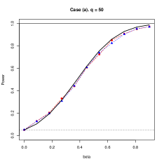
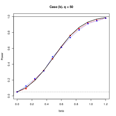
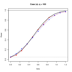
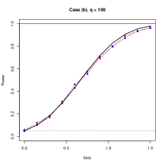
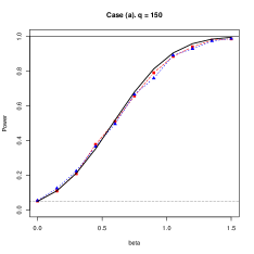
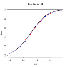
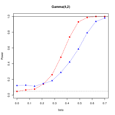
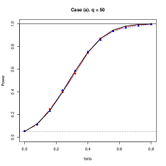
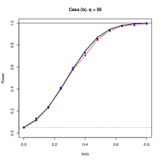
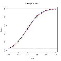
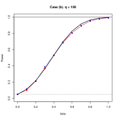
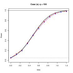
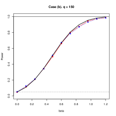
In this section, we conduct a numerical study to evaluate the finite-sample performance of our test. The simulation design follows the setting in Example 2.4 with dimensions , the number of populations , and the sample sizes randomly picked from . The populations have the structure as in Assumption 1, where the noise has i.i.d. entries with zero mean and unit variance. Moreover, we consider two different types of noises, namely the standard normal noise and the Gamma noise .
Recall that in Example 2.4, the last population is a single outlier . In this section, we set , and the other populations are all proportional to . Here, the variable will vary from to a positive number , which is selected according to different settings to control a proper increasing rate of the power. Given two non-negative definite matrices and , we define
which are the respective normalizations of and . The aim of the normalization procedure is to ensure and , which helps reduce the theoretic curve of power in (2.25) to be
| (2.26) |
where and .
The following combinations of and are considered:
(a) , and , where the first entries equal to and is a randomly chosen orthogonal matrix;
(b) and , where and are two independently and randomly chosen orthogonal matrices, and are diagonal matrices with their entries randomly picked from the interval , respectively.
For , we randomly pick a factor uniformly from and set . For each from to with step size , we repeat simulations times for the two cases of , each with two different noises, and compute the empirical size and power. The empirical sizes under (or equivalently, ) are shown in Table 1, and the curves of both theoretical and empirical powers are displayed in Figure 1. It can be observed that our proposed testing statistic controls the size well under the null case and effectively rejects when the outlier covariance matrix gradually deviate from . Also, the empirical power curves approximate the theoretical ones closely, which supports our previous theoretical analysis.
| Case (a) | Case (b) | |||
|---|---|---|---|---|
| Normal | Gamma | Normal | Gamma | |
3 A specification test for transposable data
3.1 A specification test for Kronecker product dependence structure
Transposable data is a special class of matrix-valued data whose rows and columns represent two different sets of variables [3, 4]. Recent studies of transposable data can be found in various areas such as genomics analysis and longitudinal data in financial markets, for example [27, 36, 22, 21].
Modeling dependence between rows and columns has primary importance in transposable data analysis. A widely adopted model for this purpose is the Kronecker product dependence structure, where the transposable data satisfies
| (3.1) |
where is a row covariance matrix, is a column covariance matrix, and is a random matrices having i.i.d. entries with zero mean and unit variance. Note that for and , . Hence, the covariance matrix of the vectorization of the transposable data is , namely the Kronecker product of row and column covariance matrices (this covariance structure is also referred as separable covariance model in some other fields). According to [37], “… the matrix-variate normal distribution … is widely used to model high-dimensional transposable data” (p.1310), and this type of distribution does have the Kronecker product covariance structure. Readers are referred to [37] for more justifications of the Kronecker product structure assumption.
There is an unexpectedly interesting relationship between the Kronecker dependence structure and the framework of many-sample tests we consider in the paper. To see this, let us enlarge the model into a generic independent component model (ICM) is defined as follows. A transposable data follows an ICM if , where is a non-negative definite matrix and is a -dimensional random vector having i.i.d. entries with zero mean and unit variance. Clearly, the Kronecker product structure model is a sub-model of ICM with and .
An important problem for transposable data is to test the following hypothesis
| (3.2) |
This is referred to as the diagonal hypothesis for the between-column covariance matrix , see [37]. Lemma 3.1 below establishes the connection between this diagonal hypothesis under Kronecker product structure and the many-sample proportionality test introduced in Section 2.
Lemma 3.1.
Suppose that a transposable data follows ICM. Then, the following three statements are equivalent.
(i) satisfies (3.1) with a diagonal ;
(ii) satisfies (3.1) with independent columns;
(iii) The columns of are independent and their covariance matrices are proportional to each other.
The proof of the lemma is provided in Appendix E. By Lemma 3.1, the diagonality hypothesis (item (i)) under the Kronecker product structure is equivalent to the proportionality hypothesis we considered in Section 2 for independent columns (item (iii)). This connection enables the use of our test for the diagonality hypothesis . Recall that one advantage of our test is that both dimensions and are allowed to grow to infinity with the sample size .
Let be an i.i.d. sample from a transposable population . By Lemma 3.1, our procedure of testing for the hypothesis (3.2) is summarized as follows:
(1) Let be the th column of , for and . Define , .
(2) Compute the value of the test statistic and the asymptotic variance estimate defined in Section 2.3.
(3) With significance level , reject if , where is the th upper-quantile of the standard normal.
3.2 Comparison with test in [37]
The procedure proposed in [37] for the diagonality hypothesis (3.2) is based on the key fact that under , has independent columns. Let be the th column of . Note that under the Kronecker product structure, we have for any . Thus, under ,
for any . In other words, the between column covariance matrix is diagonal. Based on this observation, [37] proposed a test statistic as an unbiased estimator for the sum of squares of the off-diagonal elements of , namely,
where stands for the Hadamard product of matrices,
Although both our procedure and the test in [37] are valid for testing the hypothesis , the two tests have different focuses. Our test statistic focuses on detection of non-proportionality of column covariance matrices while the test statistic is more sensible to detect dependence between columns. The Venn diagram in Figure 2 helps further illustrate this difference.
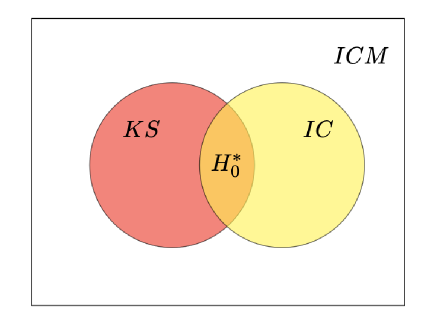
Our procedure is more sensible of alternatives lying in the yellow region where the transposable data has independent columns whose covariance matrices are not mutually proportional (this implies that the data does not follow the Kronecker product structure). In this region, the procedure in [37] might accept since is likely to have low values for independent columns. On the other hand, the procedure with is more powerful for the detection of alternatives in the red region where the transposable data does have the Kronecker product structure with however dependent columns. Indeed in this situation, our test statistic based on non-proportionality between column covariance matrices will show a low value and is more likely to accept because the column covariance matrices are still proportional under the Kronecker product structure. To summarize, for testing the hypothesis , if one believes that the covariance matrices of columns are not proportional, then our procedure is preferable. Otherwise, the proportionality of column covariance matrices is accepted and the procedure in [37] is preferable.
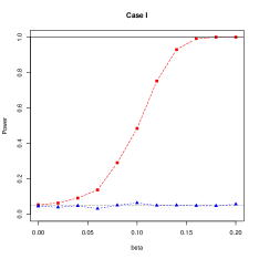
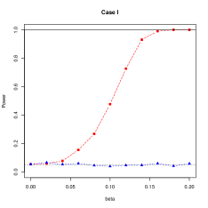
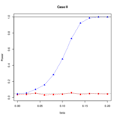
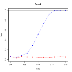
To support our assertions, we conduct a simulation study under the following setting: , , and the common sample size . The following two scenarios are considered.
-
•
Case I: The matrix-valued population consists of mutually independent columns with as in Assumption 1. The population covariance matrix , in which, for , the basis with a random orthogonal matrix and a diagonal matrix with entries randomly picked from such that are non-proportional, and are randomly selected positive weights in . When , the populations are proportional to so holds. When deviates from , the populations become non-proportional.
-
•
Case II: The matrix-valued population satisfies the Kronecker product dependence structure , where with positive weights in and a -dimensional vector having its th position one and rest positions zero, . When , is diagonal, implying that all these columns are mutually independent with their covariance matrices proportional to each other. When , columns become dependent but keep the column covariance matrices mutually proportional.
In summary, Case I maintains column independence but alters the proportionality of column covariance matrices, whereas Case II changes column dependence but keeps the proportionality of column covariance matrices unchanged. Besides, two different types of noises are also considered: the normal noise and the gamma noise .
Under these two scenarios with two different types of noise, we computed both our test statistic and the one in [37] over 1000 iterations and the empirical power curves plotted in Figure 3. In Case I, our test shows significant power, while the power of the test in [37] fluctuates around 0.05 even when the alternative does not hold. This indicates the sensitivity of the many-sample proportionality test to covariance proportionality. In Case II, our test is not sensitive to the variations in column dependence, keeping its power around 0.05. However, the test in [37] efficiently detects the change in column dependence and demonstrates significant power. These results support our previously mentioned assertions.
3.3 Analysis of the mouse aging data
Following [37], we analyze the gene dataset of Mouse Aging Project collected in [41], which measures gene expression levels from genes in up to tissues for mice (). [37] examined the dependence structure of genes expression levels among tissues () by testing the diagonality of , assuming the Kronecker product dependence structure (3.1). Their test accepted the diagonality hypothesis (3.2). However, applying our specification test presented in Section 3.1 to this hypothesis leads to the statistics value , which is much larger than the standard normal quantile; so the hypothesis is strongly rejected. Therefore, the two tests lead to significantly contradictory conclusions!
To elucidate this, according to the discussion in Section 3.2, we see that the procedure in [37] essentially tests the hypothesis that the columns from the tissues are independent; so their conclusion is indeed to accept the independence of the columns. According to Lemma 3.1, if, in addition, the Kronecker product structure (3.1) is also true, then the column covariance matrices must be proportional, which is a fact strongly rejected by our test. Therefore, the only plausible explanation is that the tissue populations are independent while the whole data set does not follow the Kronecker product structure (3.1). To recap, we conclude that gene expression levels among tissues are independent but their covariance matrices are not proportional, and the Kronecker product covariance model (3.1) is not appropriate for this mouse aging data set although the model is widely used in many studies about the dataset.
Remark 3.1.
One may wonder that the number of mouse groups is (number of samples) which is not very large and that our asymptotic results for the specification test might not be accurate. Following the recent literature in high-dimensional statistics [6, 40], high-dimensional effects take place if the ratio of dimension-to-sample-size is away from zero even though both the dimension and the sample size are not very large. In our situation, the effects of many samples can be visible if the ratio of sample number to sample size is away from zero: here we have indeed. It can be expected that the asymptotic results assuming fixed might be less accurate than our many-sample asymptotic results that consider and growing to infinity in comparable magnitude.
To further verify that our specification test is already accurate enough even for relatively small population number and sample sizes, we conduct a small simulation experiment with dimensions and sample sizes matching those of the mouse aging data, namely, , and , where other design parameters follow those of the experiments (a) and (b) in Section 2.5. The empirical sizes of the test under different settings are reported in Table 2. It can be observed that our proposed test controls the size well under the null. This thus confirms the accuracy of the asymptotic null distribution of the test statistic we derived under the many-sample framework even though the sample number and the sample sizes are not very large.
| Case (a) | Case (b) | ||
| Normal | Gamma | Normal | Gamma |
Remark 3.2.
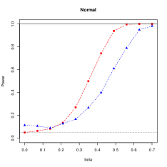
For the case of a small number of populations (), it is of special interest to compare our proposed method with existing methods for a fixed number of populations. Here, we make the comparison with a recent study [2] that addresses multi-sample tests for the proportionality of large-dimensional covariance matrices. In [2], the author proposed a -dimensional random vector to characterize the mutual proportionality among groups and proved that the null distribution of asymptotically follows a -dimensional standard normal distribution. Thus, the inner product converges to a chi-square distribution with degrees of freedom under the null.
In the simulation, we evaluate both size control and power by comparing our proportionality test with the method in [2] under the same settings: and as in the mouse aging data. We keep populations to be mutually independent and the th population satisfies the structure as in Assumption 1, with two different types of noises : and . For , the population covariance matrix , where for with a random orthogonal matrix and a diagonal matrix with entries randomly picked from such that are not proportional to each other, and are randomly selected positive weights in . It can be easily seen that the covariance matrices of these populations are proportional to when . As increases, the covariance matrices become non-proportional.
Under both the normal and the gamma noise settings, we compute both our test statistic and the statistic in [2] repeatedly for 1000 iterations and derive the empirical sizes table in Table 3 and the empirical power curves plotted in Figure 4. The results demonstrate that, although the number of populations is small, our test effectively controls the size, whereas the method in [2] fails to do so. Additionally, our test procedure shows a faster increase in power towards one as it deviates from the null hypothesis compared to the method in [2]. These findings validate the efficiency of our many-sample test procedure.
| many-sample test | proportionality test in [2] | ||
|---|---|---|---|
| Normal | Gamma | Normal | Gamma |
4 Testing of equality
4.1 Basic settings
Let be -dimensional random vectors with covariance matrix , . Consider the following equality test:
for some unknown non-negative definite matrix . For two matrices and , define . It is easy to see that characterizes the equality of two matrices. Similar to Section 2, we define
| (4.1) |
Then, the testing problem can be equivalently transferred to
| (4.2) |
We construct the test statistic in (4.3) based on an unbiased estimation of the distances ’s and the quantity .
Testing the equality hypothesis (4.2) is, in fact, simpler than testing the proportionality hypothesis analyzed in the previous sections. By repeating a similar analysis, we can construct a test statistic for the many-sample testing of the equality hypothesis. The same Assumptions 4—1 given in Section 2 will be used. For each , assume that there are independent observations from population . Let be the data matrix and the sample covariance matrix defined as in (2.1).
4.2 Unbiased estimation of the distance
The subsection parallels Section 2.2. Hence, we omit the details and directly state the final result.
Recall that, for any ,
where for . It should be noted that the second-order spectral moment of the sample covariance matrix is biased to that of the corresponding population covariance matrix due to the high-dimensional effects . Hence, we apply the unbiased estimator in (2.8) and define
| (4.3) |
It is easy to see from the discussion in Lemma 2.3 and the fact that is indeed an unbiased estimator for the distance .
4.3 The test statistic and its asymptotic normality
The proposed test statistic is given as
An immediate consequence of the discussion in Section 4.2 is that is an unbiased estimator of the quantity , i.e., . In particular, when holds, all distances and this .
To optimize the computational complexities, an explicit representation of is also given as follows:
| (4.4) |
It can be seen from the expression that the summations over two distinct indices are reduced, and the final result only involves mean values of numbers or matrices. So, the computational time is significantly shortened.
The following theorem reveals the asymptotic normality of our proposed statistic under both the null and the alternative.
Theorem 4.1.
where the inner product is defined as in (2.15).
The proof of the theorem is provided in Appendix F.1. From the above theorem, we see that the asymptotic variance can be decomposed into two parts , in which
| (4.6) |
Under Assumptions 1—3, is always positive and has both upper and lower bounds. The remainder remains non-negative. In particular, when holds, we see directly from (4.5) that for all and thus vanishes. Thus, as a direct consequence of Theorem 4.1, we have
To estimate the asymptotic variance , we define
In summary, the procedure for testing in (4.2) at significance level is to reject if , where is the th upper-quantile of the standard normal.
4.4 Power under alternative hypothesis
This section is devoted to analyzing the power of our proposed test procedure under the alternative in (4.2). The next theorem reveals the asymptotic representation of the power function and a sufficient and necessary condition for a strong rejection.
Theorem 4.4.
The proof of the theorem is mainly based on the previous Theorems 4.1 and 4.3 and is provided in Appendix G.
Remark 4.1.
Similar to Remark 2.1, we define . Then, the testing power vanishes if . In other words, a necessary condition to ensure the power is that the convergence rate of to cannot be faster than .
Theorem 4.4 that the divergence of the mean drift guarantees the power. Thus, we investigate examples parallel to those in Section 2.4 to get respective sufficient conditions.
Example 4.1 ( matrices without equal pair).
Suppose that for any , . Let . Then, the converge rate of influences the power. Since , according to Theorem 4.4, the power function tends to when .
The next example focuses on the case where the populations can be divided into subgroups, where populations within the same group are equal to each other while populations from different groups are not.
Example 4.2 (Unequal subgroups without dominant group).
Let be a positive integer smaller than and may vary as increases. Suppose that can be split into non-empty disjoint subsets . Furthermore, we assume that there are distinct non-negative definite matrices such that if . We denote . Still, is positive for fixed , but it can decrease to zero as varies. Same as Example 2.2, we use stands for the number of elements in , and assume that condition (2.21) holds, which suggests It implies that none of the groups will be dominant.
We show that the divergence of the mean drift is determined by and . Observe that
Thus, if , the value of our power function will tend to .
The next example considers the scenario with , in which the total populations consist of a dominant subgroup with a small number of outliers.
Example 4.3 (One dominant group with a few outliers).
Suppose that there exists a non-empty subset and an un-specified basis matrix such that populations outside all equal to , but within the subset, populations are not. We denote . Here, is positive for any fixed but may decrease to zero as grows.
We still focus on the small- setting: , where is the number of elements in . This assumption causes that the term in (4.6) and thus . It then follows that (4.7) can be further simplified as
| (4.8) |
We denote and . Under Assumptions 2, 3 and the small- condition, it is easy to show that both and have positive upper and lower bounds. The asymptotic variance can be simplified as .
Observe that
Therefore, in (4.8), we have
Hence, if , then and thus the power will eventually tend to .
Finally, we consider the problem of “finding a needle in a haystack”, where there is a single outlier among these populations. The relevant results will later be used in Section 4.5.
Example 4.4 (Finding a needle in a haystack).
Consider the following alternative:
| (4.9) |
where . Here, , a non-negative variable, is introduced to control the degree of deviation of from in a way that when , and gradually deviates from and as grows.
For , since there is only a single outlier, we have we have
In addition, the mean drift
Meanwhile, we also have and
Combining with (4.8), the power function now becomes
| (4.10) |
Thus, if , value of the power function will gradually tend to one.
4.5 Simulation results
The simulation design follows the settings in Example 4.4. Similar to Section 2.5, we set , the number of populations , and the sample sizes randomly picked from . We consider the standard normal noise and the Gamma noise .
In Example 4.4, we set the last population as the unique outlier (), of which , and the other populations are all identical to the matrix . Here, the parameter varies from to a selected positive number according to different scenarios. In addition, for two given distinct non-negative definite matrices and , we define
The normalization procedure helps reduce the theoretic curve in (4.10) to be
| (4.11) |
where .
The following three scenarios of and are considered:
(a) , and , where the first entries equal to and is a randomly chosen orthogonal matrix;
(b) and , where and are two independently and randomly chosen orthogonal matrices, and are diagonal matrices with their entries randomly picked from the interval .
For each from to with step size , we repeat simulations times and compute the empirical size and power. The empirical sizes are shown in Table 4, and the curves of empirical power are displayed in Figure 5. Our proposed statistic well controls the empirical size under , and effectively rejects when the outlier covariance matrix deviates from the majority as increases. Meanwhile, the empirical power curves are very close to the theoretical ones, which agrees with our previous theoretical results.
| Case (a) | Case (b) | |||
|---|---|---|---|---|
| Normal | Gamma | Normal | Gamma | |
4.6 The 1000 Genomes Project (phase 3)
The equality assumption on covariance matrices is often assumed in performing analysis of variance or covariance (ANOVA) in genetic data analysis; see for example, [28] and [29]. We here aim to check the validity of such an assumption by investigating a gene dataset from the 1000 Genomes Project phase 3 in [13]. The dataset contains phased genotypes for genes in the th chromosome of individuals from populations. The list of abbreviations, names, and sample sizes of the populations is provided below in Table 5.
| Abbreviation | Name | Size |
|---|---|---|
| ACB | (African Caribbean in Barbados) | 96 |
| ASW | (African ancestry in Southwest USA) | 61 |
| BEB | (Bengali in Bangladesh) | 86 |
| CDX | (Chinese Dai in Xishuangbanna,China) | 93 |
| CEU | (Utah residents with Northern and | 99 |
| Western European ancestry) | ||
| CHB | (Han Chinese in Beijing, China) | 103 |
| CHS | (Southern Han Chinese, China) | 105 |
| CLM | (Colombian in Medellin, Colombia) | 94 |
| ESN | (Esan in Nigeria) | 99 |
| FIN | (Finnish in Finland) | 99 |
| GBR | (British in England and Scotland) | 91 |
| GIH | (Gujarati Indian in Houston, Texas) | 103 |
| GWD | (Gambian in Western Division,The Gambia) | 113 |
| IBS | (Iberian populations in Spain) | 107 |
| ITU | (Indian Telugu in the UK) | 102 |
| JPT | (Japanese in Tokyo,Japan) | 104 |
| KHV | (Kinh in Ho Chi Minh City,Vietnam) | 99 |
| LWK | (Luhya in Webuye,Kenya) | 99 |
| MSL | (Mende in Sierra Leone) | 85 |
| MXL | (Mexican ancestry in Los Angeles,California) | 64 |
| PEL | (Peruvian in Lima,Peru) | 85 |
| PJL | (Punjabi in Lahore,Pakistan) | 96 |
| PUR | (Puerto Rican in Puerto Rico) | 104 |
| STU | (Sri Lankan Tamil in the UK) | 102 |
| TSI | (Toscani in Italy) | 107 |
| YRI | (Yoruba in Ibadan,Nigeria) | 108 |
| total | 2504 |
Assume that populations are mutually independent and for each population, the data are i.i.d. samples from the following model:
where stands for the th sample for the th population, and stand for the population-specific mean and covariance matrix, and are i.i.d. random vectors having i.i.d. entries with zero mean, unit variance and finite eighth moments. Our focus is on checking the validity of the equality hypothesis: “”.
As the ultra-high dimension of the observations is much larger than the sample sizes, a sub-sampling method is used to investigate the equality of reduced population covariance matrices with size . In other words, we repeat the experiment times. In each experiment, we randomly draw genes from the total of ones, centralize the data by the sample mean for each population, perform our testing of equality for sub-covariance matrices, and compute the values of our testing statistic. This reduction to sub-matrices indeed makes sense since the global equality hypothesis “”implies the equality of reduced covariance matrices from sub-sampled genes, and that all the test statistics is asymptotically standard normal.
It turns out that our testing statistic in these experiments ranges from to with mean , which are far greater than the standard normal quantile and thus lead to a full and strong rejection of the global equality hypothesis. Consequently, we conclude that it is indeed not reasonable to assume the equality of the population covariance matrices in this 1000 Genomes Project phase 3 dataset.
Furthermore, we investigate the contributions of different pairs of populations to the extremely large values of our statistics. Let us take a closer look at our testing statistic
where , and are given in (4.3), (4.3) and (4.3), respectively. Here, represents the contribution of the th and th populations. Indeed, according to discussions in Section 4.2 and 4.3, is an unbiased and consistent estimator for and is a consistent estimator for
in which the latter can be viewed as a global normalizer. Denote be the averaging value of over the above-mentioned repeated experiments: this statistic is, in fact, the two-sample statistic if we were, testing the single hypothesis “” and a large value means that the two covariance matrices are likely distinct.
We find that the values of ’s vary from to with a mean of . Moreover, we also classify the values of ’s into four classes by comparing them with the sample quartiles and . Figure 6 displays a heat map with these classes for all the population pairs (the diagonal entries are set to zero) where the populations are sorted according to their row averages in a decreasing order.
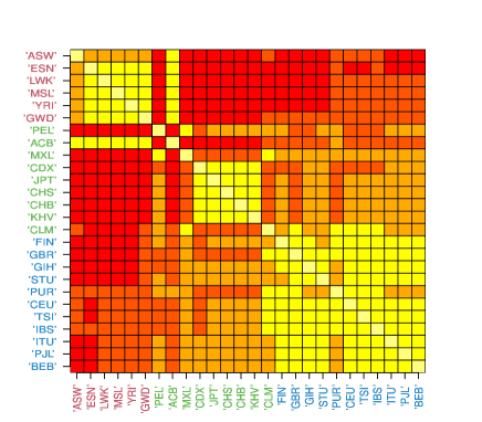
According to Figure 6, we can divide populations into three sub-groups based on their contributions to the extremely large value of our testing statistic. The main contributions come from the following six populations: “ASW”, “ESN”, “LWK”,“MSL”,“YRI” and “GWD”. It can be seen that these six deviate significantly from others since the corresponding statistic values almost always lie beyond the third quartile . Besides, there are also nine populations with medium contributions since their corresponding statistic values mostly lie between the second and third quartiles. The other eleven populations tend to take smaller values below the first quartile, though they are still not small enough to allow us to treat their covariance matrices as equal.
[Acknowledgments] The authors wish to express their appreciation to the anonymous reviewers, the Associate Editor, and the Editor for their insightful feedback and constructive suggestions, which have greatly contributed to the improvement of this paper.
Chen Wang was partially supported by Hong Kong RGC General Research Fund 17301021 and National Natural Science Foundation of China Grant 72033002. Jianfeng Yao was partially supported by NSFC RFIS Grant No. 12350710179.
Supplement to “Many-sample tests for the equality and the proportionality hypotheses between large covariance matrices” \sdescriptionIn this supplement, we provide all technical proofs.
References
- Ahmad [2017] {barticle}[author] \bauthor\bsnmAhmad, \bfnmM. R.\binitsM. R. (\byear2017). \btitleLocation-invariant Multi-sample U-tests for Covariance Matrices with Large Dimension. \bjournalScandinavian Journal of Statistics \bvolume44 \bpages500-523. \endbibitem
- Ahmad [2022] {barticle}[author] \bauthor\bsnmAhmad, \bfnmRauf\binitsR. (\byear2022). \btitleTests for proportionality of matrices with large dimension. \bjournalJournal of Multivariate Analysis \bvolume189 \bpages104865. \bdoihttps://doi.org/10.1016/j.jmva.2021.104865 \endbibitem
- Allen and Tibshirani [2010] {barticle}[author] \bauthor\bsnmAllen, \bfnmG. I.\binitsG. I. and \bauthor\bsnmTibshirani, \bfnmR.\binitsR. (\byear2010). \btitleTransposable regularized covariance models with an application to missing data imputation. \bjournalThe Annals of Applied Statistics \bvolume4 \bpages764–790. \endbibitem
- Allen and Tibshirani [2012] {barticle}[author] \bauthor\bsnmAllen, \bfnmG. I.\binitsG. I. and \bauthor\bsnmTibshirani, \bfnmR.\binitsR. (\byear2012). \btitleInference with transposable data: Modelling the effects of row and column correlations. \bjournalJournal of the Royal Statistical Society B (Statistical Methodology) \bvolume74 \bpages721–743. \endbibitem
- Bai et al. [2009a] {barticle}[author] \bauthor\bsnmBai, \bfnmZ.\binitsZ., \bauthor\bsnmJiang, \bfnmD.\binitsD., \bauthor\bsnmYao, \bfnmJ. F.\binitsJ. F. and \bauthor\bsnmZheng, \bfnmS.\binitsS. (\byear2009a). \btitleCorrections to LRT on large-dimensional covariance matrix by RMT. \bjournalThe Annals of Statistics \bvolume37 \bpages3822-3840. \endbibitem
- Bai et al. [2009b] {barticle}[author] \bauthor\bsnmBai, \bfnmZhidong\binitsZ., \bauthor\bsnmJiang, \bfnmDandan\binitsD., \bauthor\bsnmYao, \bfnmJian-Feng\binitsJ.-F. and \bauthor\bsnmZheng, \bfnmShurong\binitsS. (\byear2009b). \btitleCorrections to LRT on large-dimensional covariance matrix by RMT. \bjournalThe Annals of Statistics \bvolume37 \bpages3822–3840. \endbibitem
- Bai et al. [2021] {barticle}[author] \bauthor\bsnmBai, \bfnmZ.\binitsZ., \bauthor\bsnmHu, \bfnmJ.\binitsJ., \bauthor\bsnmWang, \bfnmC.\binitsC. and \bauthor\bsnmZhang, \bfnmC.\binitsC. (\byear2021). \btitleTest on the linear combinations of covariance matrices in high-dimensional data. \bjournalStatistical Papers \bvolume62 \bpages701-719. \endbibitem
- Bao and Ullah [2010] {barticle}[author] \bauthor\bsnmBao, \bfnmYong\binitsY. and \bauthor\bsnmUllah, \bfnmAman\binitsA. (\byear2010). \btitleExpectation of quadratic forms in normal and nonnormal variables with applications. \bjournalJournal of Statistical Planning and Inference \bvolume140 \bpages1193 – 1205. \bdoi10.1016/j.jspi.2009.11.002 \endbibitem
- Butucea and Zgheib [2017] {barticle}[author] \bauthor\bsnmButucea, \bfnmC.\binitsC. and \bauthor\bsnmZgheib, \bfnmR.\binitsR. (\byear2017). \btitleAdaptive test for large covariance matrices in presence of missing observations. \bjournalAlea (Rio de Janeiro) \bvolume14 \bpages557-578. \endbibitem
- Chen, Zhang and Zhong [2010] {barticle}[author] \bauthor\bsnmChen, \bfnmS. X.\binitsS. X., \bauthor\bsnmZhang, \bfnmL. X.\binitsL. X. and \bauthor\bsnmZhong, \bfnmP. S.\binitsP. S. (\byear2010). \btitleTests for high-dimensional covariance matrices. \bjournalJournal of the American Statistical Association \bvolume105 \bpages810-819. \endbibitem
- Cheng et al. [2020] {barticle}[author] \bauthor\bsnmCheng, \bfnmG.\binitsG., \bauthor\bsnmLiu, \bfnmB.\binitsB., \bauthor\bsnmTian, \bfnmG.\binitsG. and \bauthor\bsnmZheng, \bfnmS.\binitsS. (\byear2020). \btitleTesting proportionality of two high-dimensional covariance matrices. \bjournalComputational Statistics and Data Analysis \bvolume150. \bdoi10.1016/j.csda.2020.106962 \endbibitem
- Coelho and Marques [2012] {barticle}[author] \bauthor\bsnmCoelho, \bfnmC. A.\binitsC. A. and \bauthor\bsnmMarques, \bfnmF. J.\binitsF. J. (\byear2012). \btitleNear-exact distributions for the likelihood ratio test statistic to test equality of several variance-covariance matrices in elliptically contoured distributions. \bjournalComputational Statistics \bvolume27 \bpages627-659. \endbibitem
- 1000 Genomes Project Consortium [2015] {barticle}[author] \bauthor\bsnm1000 Genomes Project Consortium (\byear2015). \btitleA global reference for human genetic variation. \bjournalNature \bvolume526 \bpages68-74. \bdoi10.1038/nature15393 \endbibitem
- Fisher, Sun and Gallagher [2010] {barticle}[author] \bauthor\bsnmFisher, \bfnmT. J.\binitsT. J., \bauthor\bsnmSun, \bfnmX.\binitsX. and \bauthor\bsnmGallagher, \bfnmC. M.\binitsC. M. (\byear2010). \btitleA new test for sphericity of the covariance matrix for high dimensional data. \bjournalJournal of Multivariate Analysis \bvolume101 \bpages2554-2570. \endbibitem
- Friendly and Sigal [2020] {barticle}[author] \bauthor\bsnmFriendly, \bfnmM.\binitsM. and \bauthor\bsnmSigal, \bfnmM.\binitsM. (\byear2020). \btitleVisualizing Tests for Equality of Covariance Matrices. \bjournalAmerican Statistician \bvolume74 \bpages144-155. \endbibitem
- Han and Wu [2021] {barticle}[author] \bauthor\bsnmHan, \bfnmY.\binitsY. and \bauthor\bsnmWu, \bfnmW. B.\binitsW. B. (\byear2021). \btitleTest for high dimensional covariance matrices. \bjournalAnnals of Statistics \bvolume48 \bpages3565-3588. \endbibitem
- Ishii, Yata and Aoshima [2019] {barticle}[author] \bauthor\bsnmIshii, \bfnmA.\binitsA., \bauthor\bsnmYata, \bfnmK.\binitsK. and \bauthor\bsnmAoshima, \bfnmM.\binitsM. (\byear2019). \btitleEquality tests of high-dimensional covariance matrices under the strongly spiked eigenvalue model. \bjournalJournal of Statistical Planning and Inference \bvolume202 \bpages99-111. \endbibitem
- Jiang, Jiang and Yang [2012] {barticle}[author] \bauthor\bsnmJiang, \bfnmD.\binitsD., \bauthor\bsnmJiang, \bfnmT.\binitsT. and \bauthor\bsnmYang, \bfnmF.\binitsF. (\byear2012). \btitleLikelihood ratio tests for covariance matrices of high-dimensional normal distributions. \bjournalJournal of Statistical Planning and Inference \bvolume142 \bpages2241-2256. \endbibitem
- Ledoit and Wolf [2002] {barticle}[author] \bauthor\bsnmLedoit, \bfnmO.\binitsO. and \bauthor\bsnmWolf, \bfnmM.\binitsM. (\byear2002). \btitleSome hypothesis tests for the covariance matrix when the dimension is large compared to the sample size. \bjournalAnnals of Statistics \bvolume30 \bpages1081-1102. \endbibitem
- Ledoit and Wolf [2017] {barticle}[author] \bauthor\bsnmLedoit, \bfnmOlivier\binitsO. and \bauthor\bsnmWolf, \bfnmMichael\binitsM. (\byear2017). \btitleNumerical implementation of the QuEST function. \bjournalComputational Statistics & Data Analysis \bvolume115 \bpages199–223. \endbibitem
- Lee, Daniels and Joo [2013] {barticle}[author] \bauthor\bsnmLee, \bfnmK.\binitsK., \bauthor\bsnmDaniels, \bfnmM. J.\binitsM. J. and \bauthor\bsnmJoo, \bfnmY.\binitsY. (\byear2013). \btitleFlexible marginalized models for bivariate longitudinal ordinal data. \bjournalBiostatistics \bvolume14 \bpages462-476. \bdoi10.1093/biostatistics/kxs058 \endbibitem
- Leng and Tang [2012] {barticle}[author] \bauthor\bsnmLeng, \bfnmC.\binitsC. and \bauthor\bsnmTang, \bfnmC. Y.\binitsC. Y. (\byear2012). \btitleSparse matrix graphical models. \bjournalJournal of the American Statistical Association \bvolume107 \bpages1187-1200. \bdoi10.1080/01621459.2012.706133 \endbibitem
- Li and Chen [2012] {barticle}[author] \bauthor\bsnmLi, \bfnmJ.\binitsJ. and \bauthor\bsnmChen, \bfnmS. X.\binitsS. X. (\byear2012). \btitleTwo sample tests for high-dimensional covariance matrices. \bjournalAnnals of Statistics \bvolume40 \bpages908-940. \endbibitem
- Li and Yao [2016] {barticle}[author] \bauthor\bsnmLi, \bfnmZ.\binitsZ. and \bauthor\bsnmYao, \bfnmJ.\binitsJ. (\byear2016). \btitleTesting the sphericity of a covariance matrix when the dimension is much larger than the sample size. \bjournalElectronic Journal of Statistics \bvolume10 \bpages2973-3010. \endbibitem
- Liao, Peng and Zhang [2021] {barticle}[author] \bauthor\bsnmLiao, \bfnmG.\binitsG., \bauthor\bsnmPeng, \bfnmL.\binitsL. and \bauthor\bsnmZhang, \bfnmR.\binitsR. (\byear2021). \btitleEmpirical likelihood test for the equality of several high-dimensional covariance matrices. \bjournalScience China Mathematics \bvolume64 \bpages2775-2792. \endbibitem
- Liu et al. [2013] {barticle}[author] \bauthor\bsnmLiu, \bfnmB.\binitsB., \bauthor\bsnmXu, \bfnmL.\binitsL., \bauthor\bsnmZheng, \bfnmS.\binitsS. and \bauthor\bsnmTian, \bfnmG. L.\binitsG. L. (\byear2013). \btitleA new test for the proportionality of two large-dimensional covariance matrices. \bjournalJournal of Multivariate Analysis \bvolume131 \bpages293-308. \endbibitem
- Ning and Liu [2013] {barticle}[author] \bauthor\bsnmNing, \bfnmY.\binitsY. and \bauthor\bsnmLiu, \bfnmH.\binitsH. (\byear2013). \btitleHigh-dimensional semiparametric bigraphical models. \bjournalBiometrika \bvolume100 \bpages655-670. \bdoi10.1093/biomet/ast009 \endbibitem
- Patterson, Price and Reich [2006] {barticle}[author] \bauthor\bsnmPatterson, \bfnmN.\binitsN., \bauthor\bsnmPrice, \bfnmA. L.\binitsA. L. and \bauthor\bsnmReich, \bfnmD.\binitsD. (\byear2006). \btitlePopulation structure and eigenanalysis. \bjournalPLoS Genetics \bvolume2 \bpages2074-2093. \bdoi10.1371/journal.pgen.0020190 \endbibitem
- Price et al. [2006] {barticle}[author] \bauthor\bsnmPrice, \bfnmA. L.\binitsA. L., \bauthor\bsnmPatterson, \bfnmN. J.\binitsN. J., \bauthor\bsnmPlenge, \bfnmR. M.\binitsR. M., \bauthor\bsnmWeinblatt, \bfnmM. E.\binitsM. E., \bauthor\bsnmShadick, \bfnmN. A.\binitsN. A. and \bauthor\bsnmReich, \bfnmD.\binitsD. (\byear2006). \btitlePrincipal components analysis corrects for stratification in genome-wide association studies. \bjournalNature Genetics \bvolume38 \bpages904-909. \bdoi10.1038/ng1847 \endbibitem
- Qiu and Chen [2012] {barticle}[author] \bauthor\bsnmQiu, \bfnmY.\binitsY. and \bauthor\bsnmChen, \bfnmS. X.\binitsS. X. (\byear2012). \btitleTest for bandedness of high-dimensional covariance matrices and bandwidth estimatio. \bjournalAnnals of Statistics \bvolume40 \bpages1285-1314. \endbibitem
- Schott [2006] {barticle}[author] \bauthor\bsnmSchott, \bfnmJ. R.\binitsJ. R. (\byear2006). \btitleA high-dimensional test for the equality of the smallest eigenvalues of a covariance matrix. \bjournalJournal of Multivariate Analysis \bvolume97 \bpages827-843. \endbibitem
- Schott [2007] {barticle}[author] \bauthor\bsnmSchott, \bfnmJ. R.\binitsJ. R. (\byear2007). \btitleA test for the equality of covariance matrices when the dimension is large relative to the sample sizes. \bjournalComputational Statistics and Data Analysis \bvolume51 \bpages6535-6542. \endbibitem
- Srivastava, Kollo and von Rosen [2011] {barticle}[author] \bauthor\bsnmSrivastava, \bfnmM. S.\binitsM. S., \bauthor\bsnmKollo, \bfnmT.\binitsT. and \bauthor\bparticlevon \bsnmRosen, \bfnmD.\binitsD. (\byear2011). \btitleSome tests for the covariance matrix with fewer observations than the dimension under non-normality. \bjournalJournal of Multivariate Analysis \bvolume102 \bpages1090-1103. \endbibitem
- Srivastava, Yanagihara and Kubokawa [2014] {barticle}[author] \bauthor\bsnmSrivastava, \bfnmM. S.\binitsM. S., \bauthor\bsnmYanagihara, \bfnmH.\binitsH. and \bauthor\bsnmKubokawa, \bfnmT.\binitsT. (\byear2014). \btitleTests for covariance matrices in high dimension with less sample size. \bjournalJournal of Multivariate Analysis \bvolume130 \bpages289-309. \endbibitem
- Tian, Lu and Li [2015] {barticle}[author] \bauthor\bsnmTian, \bfnmX.\binitsX., \bauthor\bsnmLu, \bfnmY.\binitsY. and \bauthor\bsnmLi, \bfnmW.\binitsW. (\byear2015). \btitleA robust test for sphericity of high-dimensional covariance matrices. \bjournalJournal of Multivariate Analysis \bvolume141 \bpages217-227. \endbibitem
- Touloumis, Marioni and Tavaré [2016] {barticle}[author] \bauthor\bsnmTouloumis, \bfnmA.\binitsA., \bauthor\bsnmMarioni, \bfnmJ. C.\binitsJ. C. and \bauthor\bsnmTavaré, \bfnmS.\binitsS. (\byear2016). \btitleHDTD: Analyzing multi-tissue gene expression data. \bjournalBioinformatics \bvolume32 \bpages2193-2195. \bdoi10.1093/bioinformatics/btw224 \endbibitem
- Touloumis, Marioni and Tavaré [2021] {barticle}[author] \bauthor\bsnmTouloumis, \bfnmAnestis\binitsA., \bauthor\bsnmMarioni, \bfnmJohn C\binitsJ. C. and \bauthor\bsnmTavaré, \bfnmSimon\binitsS. (\byear2021). \btitleHypothesis Testing for the Covariance Matrix in High-Dimensional Transposable Data with Kronecker Product Dependence Structure. \bjournalStatistica Sinica \bvolume31 \bpages1–38. \bdoi10.5705/ss.202018.0268 \endbibitem
- Ullah [2004] {bbook}[author] \bauthor\bsnmUllah, \bfnmAman\binitsA. (\byear2004). \btitleFinite sample econometrics. \bpublisherNew York: Oxford University Press. \endbibitem
- Wang and Yao [2013] {barticle}[author] \bauthor\bsnmWang, \bfnmQ.\binitsQ. and \bauthor\bsnmYao, \bfnmJ.\binitsJ. (\byear2013). \btitleOn the sphericity test with large-dimensional observations. \bjournalElectronic Journal of Statistics \bvolume7 \bpages2164-2192. \endbibitem
- Yao, Zheng and Bai [2015] {bbook}[author] \bauthor\bsnmYao, \bfnmJianfeng\binitsJ., \bauthor\bsnmZheng, \bfnmShurong\binitsS. and \bauthor\bsnmBai, \bfnmZhidong\binitsZ. (\byear2015). \btitleSample covariance matrices and high-dimensional data analysis. \bpublisherCambridge University Press Cambridge. \endbibitem
- Zahn et al. [2007] {barticle}[author] \bauthor\bsnmZahn, \bfnmJ. M.\binitsJ. M., \bauthor\bsnmPoosala, \bfnmS.\binitsS., \bauthor\bsnmOwen, \bfnmA. B.\binitsA. B., \bauthor\bsnmIngram, \bfnmD. K.\binitsD. K., \bauthor\bsnmLustig, \bfnmA.\binitsA., \bauthor\bsnmCarter, \bfnmA.\binitsA., \bauthor\bsnmWeeraratna, \bfnmA. T.\binitsA. T., \bauthor\bsnmTaub, \bfnmD. D.\binitsD. D., \bauthor\bsnmGorospe, \bfnmM.\binitsM., \bauthor\bsnmMazan-Mamczarz, \bfnmK.\binitsK., \bauthor\bsnmLakatta, \bfnmE. G.\binitsE. G., \bauthor\bsnmBoheler, \bfnmK. R.\binitsK. R., \bauthor\bsnmXu, \bfnmX.\binitsX., \bauthor\bsnmMattson, \bfnmM. P.\binitsM. P., \bauthor\bsnmFalco, \bfnmG.\binitsG., \bauthor\bsnmKo, \bfnmM. S. H.\binitsM. S. H., \bauthor\bsnmSchlessinger, \bfnmD.\binitsD., \bauthor\bsnmFirman, \bfnmJ.\binitsJ., \bauthor\bsnmKummerfeld, \bfnmS. K.\binitsS. K., \bauthor\bsnmWood III, \bfnmW. H.\binitsW. H., \bauthor\bsnmZonderman, \bfnmA. B.\binitsA. B., \bauthor\bsnmKim, \bfnmS. K.\binitsS. K. and \bauthor\bsnmBecker, \bfnmK. G.\binitsK. G. (\byear2007). \btitleAGEMAP: A gene expression database for aging in mice. \bjournalPLoS Genetics \bvolume3 \bpages2326-2337. \bdoi10.1371/journal.pgen.0030201 \endbibitem
- Zhang et al. [2018] {barticle}[author] \bauthor\bsnmZhang, \bfnmC.\binitsC., \bauthor\bsnmBai, \bfnmZ.\binitsZ., \bauthor\bsnmHu, \bfnmJ.\binitsJ. and \bauthor\bsnmWang, \bfnmC.\binitsC. (\byear2018). \btitleMulti-sample test for high-dimensional covariance matrices. \bjournalCommunications in Statistics - Theory and Methods \bvolume47 \bpages3161-3177. \endbibitem
Supplement to “Many-sample tests for the equality and the proportionality hypotheses between large covariance matrices” \sdescription
Tianxing Mei, Chen Wang and Jianfeng Yao
Appendix A Auxiliary Lemmas
Let be an i.i.d. sample from a -dimensional population , where is a semi-definite matrix and has i.i.d. entries with zero mean, unit variance, finite fourth moment and finite eighth moment.
For any semi-definite matrix , and symmetric matrices and , we denote
| (A.1) |
where is a diagonal matrix made by diagonal entries of . We directly see that when is fixed, is a non-negative definite bi-linear function on the product space of symmetric matrices. Moreover, when , and are bounded uniformly in operator norm with respect to , so is .
Let be the sample covariance matrix, that is, . Here, we focus on moments of the following statistics related to :
where is a symmetric deterministic matrix. These two quantities play a crucial role in deriving the asymptotic normality of our proposed -statistic in Sections 2 and 4.
The following lemmas provide the expectations, covariances, and bounds of the fourth moment about these statistics. The proofs of the results are based on the formulas of quadratic forms of random vectors discussed in [38] and [8] with some lengthy but tedious calculations. We provide detailed proofs for some of the crucial formulas in the last Appendix H.
The first result displays the expectation formulas for the two statistics.
Lemma A.1.
Suppose that satisfies the structure given at the beginning of this section. Then, it holds that
| (A.2) |
Meanwhile, for any symmetric matrix , we also have
| (A.3) |
The next lemma provides the covariance formulas.
Lemma A.2.
Suppose that satisfies the pressumed structure. Then, we have
| (A.4) |
In addition, for symmetric matrices , and , we also have
| (A.5) |
and
| (A.6) |
Consequently, it also holds that
| (A.7) |
| (A.8) |
where .
The next lemma shows the covariances of two statistics considered in this section with a statistic in the form of .
Lemma A.3.
Let be the i.i.d. sample from the population satisfying the structure given before. Then, for any symmetric matrix , we have
| (A.9) |
and
| (A.10) |
Consequently, we have
| (A.11) |
The final results conclude the finiteness of their fourth moments.
Lemma A.4.
For given at the beginning of the section, there exists a positive constant dependent only on and the ratio such that
Meanwhile, for any symmetric matrices and that are bounded in operator norm, there is another positive constant relying only on and the operator norms of , and such that
Appendix B Proofs in Section 2.2
B.1 Proof of Lemma 2.2
Observe that for any ,
Therefore, the statistic is actually a the -statistic, i.e.,
| (B.1) |
and thus
The conclusion in Lemma 2.2 then follows.
B.2 Proof of Lemma 2.3
Let
We conclude that the matrix is invertible and next will calculate the explicit form of its inverse. Indeed, The determinant of is
With this in mind, we find the inverse of :
| (B.2) |
where stands for the adjugate of .
Hence, by solving the system of equations, we find that
We first simplify the expression of . Recall the discussion in the last section that is a -statistic and satisfies (B.1). Observe that
It then follows that
For simplicity, we denote
| (B.3) |
Appendix C Proofs in Section 2.3
C.1 Proofs of Theorem 2.4
The main idea to derive the limiting distribution of a statistic resembling a -statistic is to approximate it by its Hajeck projection. (See \citesupp[Chapters 11 and 12]vander2000 for details.)
Let be the set of all variables of the form for arbitrary measurable functions of the observations related to the -th population with . Then, the Hajéck projection of satisfies
| (C.1) |
where
| (C.2) |
It can be easily seen that is a sum of independent and centered random variables.
To show is a good approximation to , we observe that, under Assumptions 1—3, there exists a positive constant that bounds uniformly for any . (The proof of the uniform boundedness is tedious and totally similar to the discussion for the variance below, and thus omitted.) Thus, we can apply the similar argument for the -statistic of order two as in Theorem 12.3 of \citesuppvander2000 to obtain
It then follows by Theorem 11.2 in \citesuppvander2000 that
Hence, it suffices for us to prove the asymptotic normality of .
Before proceeding to the asymptotic normality of , we first simplify the representation of . Observe that
| (C.3) |
where is given in (2.11). Recall the definitions of , and given in (2.16). By (B.2), we further find
| (C.4) |
where the remainder satisfies
| (C.5) |
The Assumptions 1—3 ensure that variances of , and are all uniformly bounded by some positive constant independent of and . Therefore, variances of the remainders are also uniformly bounded and of order , that is, for another positive number, say, . Consequently, we see that
Thus, it only remains to show the asymptotic normality of the sum of ’s. Observe that ’s are mutually independent, we immediately have provided that the Lyaponouv condition
| (C.6) |
holds. Hence, it remains (i) to derive the explicit representation of in terms of the spectral moments of , and (ii) to verify the Lyaponouv condition (C.6).
Let . Then,
Hence, to achieve the goal (i), it suffices to find the explicit formula of .
Recall the definition of in (C.4). Applying Lemma A.2, we have
in which, under Assumptions 1—3, the remainders can be uniformly bounded and of order , i.e., for some constant . Adopting the notation in (2.17), we can then simplify the variance to be
Since both and are uniformly bounded under Assumptions 1—3, it is easy to see that
Also, by Assumption 2, we have
and thus
It suggests that the denominator in (C.6) satisfies
for some positive constants and .
Meanwhile, according to Lemma A.4, together with Assumptions 1—3, there exists some constant such that
| (C.7) |
which means the numerator in (C.6) has the order of . Hence, the Lyaponouv condition (C.6) indeed holds.
Combining the discussions above, we finally conclude that
where
The proof is complete.
C.2 Proof of Corollary 2.5
C.3 Proof of Theorem 2.6
According to Theorem 2.4, it only remains to show that is consistent to . From the discussion in the last Section C.1, we have already seen that both and can be uniformly bounded under Assumptions 1—3. In other words, there is a positive constant independent of and such that
Meanwhile, we recall that and are normailzed spectral moments of and as in (2.7) and (2.6), which are linear combinations of matrices
Since are uniformly bounded in Assumption 2, we know from [BS10, Theorem 5.8] that are also uniformly bounded with probability one. Consequently, there exists another constant such that for any ,
It then follows that
and
Hence, we have
Similarly,
Thus, we also have
Combining the above results with (2.19), we see that is indeed a consistent estimator for . Thus, the proof is complete.
Appendix D Proof of Theorem 2.7
According to Theorem 2.4, is still asymptotically normal under alternative, that is,
Still, according to Theorem 2.6, is always consistent to whenever holds or not. Hence, .
Observe that
which proves the first conclusion.
To see the second conclusion, we notice that is upper bounded under Assumption 2. Hence, there exists some positive constant such that . Meanwhile, since and the later has a positive lower bound under Assumption 1. In short, we have , where are positive constants. With this fact in mind, we immediately have
Meanwhile, since , we have
where the right-hand side remains unchanged when and increase. Consequently, we have
From the above discussion, it is not difficult to see that the power function (2.20) tends to if and only if . The proof is then complete.
Appendix E Proof of Lemma 3.1
“(i) (iii)”: Assume that satisfies (3.1) with diagonal. Let and be columns of and respectively. Denote be the th entry of and write be the th column of . Since satisfies (3.1), we have
Hence, columns of can be represented by linear combinations of ’s with the coefficients the corresponding columns of , that is,
When is diagonal, so is . Then, we have . It follows that are independent and their covariance matrices differ only by a factor.
“(iii)(ii)”: Assume that are independent with their covariance matrices proportional to each other. Divide into blocks of size and denote the th block by . Correspondingly, denote the th block of . Then,
and
Since and are independent for any , we have for all . Hence, for , and . Moreover, since covariance matrices of are proportional to each other, there must exists a sequence of and a matrix such that . Let and . We have and therefore .
“(ii) (i)”: Assume that satisfies (3.1) with independent columns. Note that
Due to the column independence, for any . Hence, for any . In other words, is diagonal.
Appendix F Proofs in Section 4.3
F.1 Proof of Theorem 4.1
The proof is roughly parallel to that in Section C.1, by the method of Hajéck projection. The Hajéck projection of satisfies
| (F.1) |
where
| (F.2) |
It can be easily seen that is a sum of independent variables with zero mean.
Under Assumptions 1—4, are bounded uniformly for all . Thus, we apply a similar argument as in Theorem 12.3 and Theorem 11.2 in \citesuppvander2000 to have
To simplify the representation of , we observe that
| (F.3) |
Let
Then, . With this notation, we immediately find that
| (F.4) |
where the remainder satisfies
| (F.5) |
Under Assumptions 2—3, the variances of can be uniformly bounded in the form: . Hence, we see that
Consequently, to obtain , it suffices to verify the Lyaponouv condition
| (F.6) |
F.2 Proof of Theorem 4.3
The proof is, in general, parallel to that in Section C.3. Here, we show the consistency of to , i.e., . Recall the discussion in Section C.3, are uniformly bounded with probability one, that is, there exists a uniform constant such that for any ,
It then follows that
so that
In other words,
The proof is then complete.
Appendix G Proof of Theorem 4.4
According to Theorem 4.1, is still asymptotically normal under alternative, that is,
Meanwhile, by Theorem 4.3, is always consistent to in general. In other words, .
Observe that
So, the first conclusion is proved.
As for the second conclusion, recall that is upper bounded under Assumption 2. In other words, there must be a positive constant such that . Meanwhile, we also have under Assumption 1. In total, we now see that and thus
Meanwhile, since , we have
where the right-hand side is independent of and . Consequently, we have
From the above inequality, it is easy to see that the power function (4.7) tends to if and only if . The proof is then complete.
Appendix H Proofs of Auxiliary Lemmas
H.1 Auxiliary Covariance Formulas
The proofs of results in Appendix A rely heavily on computing the covariances of products of quadratic forms of random vectors. Suppose that is a -dimensional random vector with i.i.d. entries having zero mean, unit variance, and finite fourth moment , which is independent of coordinates.
Suppose that be arbitrary deterministic symmetric matrices such that traces of all possible ’s, ’s, ’s and ’s are of . This is always the case when they are bounded in the operator norm, and their singular value distributions converge weakly to certain deterministic limits. Under this assumption, we now focus on the terms in the highest orders of the following two covariances:
and
These leading terms determine the asymptotic variances occurring in Theorems 2.4 and 4.1. The following lemma provides the corresponding answers of our interest.
Lemma H.1.
Suppose that and ’s satisfy the above-mentioned conditions. Then, we have
| (H.1) |
and
| (H.2) |
H.2 Proof of Equation (A.4)
Observe that
We have
Let us consider these four types of covariances step by step.
For the first term , by letting in (H.1), we have
Next, for the third term , we have
Since
we have
Therefore,
It remains to compute the last term .To see this, we let be the -dimensional vector with its th entry and the others . Then,
It follows that
Let . Then, we have
Consequently, it holds that
where stands for the Hadamard product of matrices. According to Corollary A.21 in \citesuppBS10, we have
so that the traces above are of order .
Back to the last term, we find
Therefore,
To recap, we have
H.3 Proof of Equation (A.5)
Recall that
We have
In what follows, we compute these different types of terms step by step.
First, by letting , and in (H.1), we have
Furthermore, we focus on the cases in which there are two different indices, and each index occurs four times. We observe that
so that
It then follows that
Similarly, we also have
Finally, we focus on the cases with three different indices. Observe that
Similarly, the other three cases satisfy
To recap, we have
H.4 Proof of Equation (A.6)
Recall that
We have
In what follows, we compute these different types of terms step by step.
First, by letting and in (H.1), we have
Next, by letting and in (H.2), we have
Meanwhile, by letting in (H.2), we have
Finally, we observe that
It then follows that
We have
Finally,
To recap, we have
H.5 Proof of Equation (A.9)
Recall that
Then, we have
H.6 Proof of Equation (A.10)
Recall that
We then have
imsart-nameyear \bibliographysuppmybibsp,mybibfile