Magnetic Dirac operator in strips
submitted to strong magnetic fields

Abstract.

We consider the magnetic Dirac operator on a curved strip whose boundary carries the infinite mass boundary condition. When the magnetic field is large, we provide the reader with accurate estimates of the essential and discrete spectra. In particular, we give sufficient conditions ensuring that the discrete spectrum is non-empty.

1. Motivations and main results

1.1. The magnetic Dirac operator on a strip

We perform the spectral analysis of magnetic Dirac operators on bidimensional strips.

The strips under consideration in this article are built from a smooth curve without self-intersections $\gamma:\mathbb{R}\to\mathbb{R}^{2}$ (with $|\gamma^{\prime}|=1$) and from the application

$$\Theta:\Omega_{0}\ni(s,t)\mapsto\gamma(s)+t\mathbf{n}(s)\,,$$ (1.1)

where $\mathbf{n}=\gamma^{\prime\perp}$ is chosen so that $(\gamma^{\prime},\bf{n})$ forms a direct orthonormal basis and $\Omega_{0}=\mathbb{R}\times(-\delta,\delta)$ is a straight strip of width $\delta>0$ so small that $\Theta$ is injective. The curvature $\kappa$ of $\gamma$ is characterized by

$$\gamma^{\prime\prime}(s)=\kappa(s)\textbf{n}(s)$$

for all $s\in\mathbb{R}$. To simplify the analysis, we only consider the case when the curvature has compact support. Then, the strip is $\Omega=\Theta(\Omega_{0})$, which, for $\delta$ small enough, is a smooth curved strip about the base curve $\gamma$ (see Figure 1).

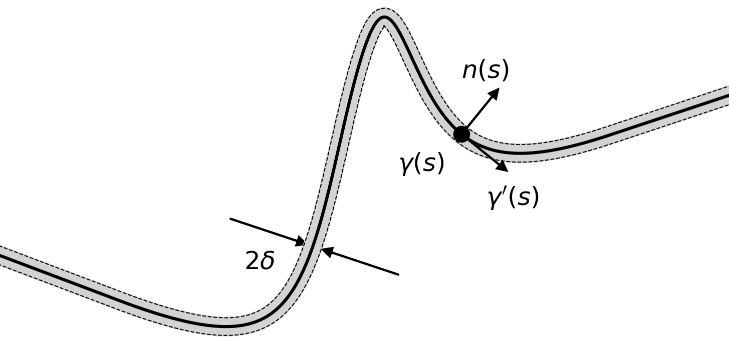
Figure 1. Typical Waveguide Profile

In order to define the Dirac operator with constant magnetic field $B=1$, we need an associated vector potential $\mathbf{A}:\overline{\Omega}\to\mathbb{R}^{2}$ (that is a function such that $\partial_{1}A_{2}-\partial_{2}A_{1}=1$). Note that any two associated vector potentials yield unitarily equivalent operators, given that $\Omega$ is simply connected. In such a geometric context, there is a rather natural choice. Consider the bounded function $\phi_{0}$ on $\Omega_{0}$ given by

$$\phi_{0}(s,t)=\frac{t^{2}-\delta^{2}}{2}\,,$$

which satisfies $\mathrm{curl}\mathbf{A}_{0}=1$, with $\mathbf{A}_{0}=\nabla\phi^{\perp}_{0}=(-t,0)$. The following proposition has been established in [4, Proposition 1.2].

Proposition 1.1.

Let $\hat{\phi}_{0}=\phi_{0}\circ\Theta^{-1}\in\mathscr{C}^{\infty}(\overline{\Omega})$. There exists a unique $\phi\in\mathscr{C}^{\infty}(\overline{\Omega})$ such that $\Delta\phi=1$, $\phi_{|\partial\Omega}=0$, and $\phi-\hat{\phi}_{0}\in\mathscr{S}(\overline{\Omega})$. Moreover, there exists $c_{0}>0$ such that $\partial_{\mathbf{N}}\phi\geqslant c_{0}$ on $\partial\Omega$, $\mathbf{N}$ being the outward pointing normal to the boundary.

Thanks to the function $\phi$ given in Proposition 1.1, we get the existence of a smooth and bounded vector potential $\mathbf{A}=\nabla\phi^{\perp}$ on the curved strip $\Omega$.

For $h>0$, we consider the magnetic Dirac operators

$$\mathscr{D}_{h}=\sigma\cdot(\mathbf{p}-\mathbf{A})=\begin{pmatrix}0&d_{h,\mathbf{A}}\\ d^{\times}_{h,\mathbf{A}}&0\end{pmatrix}=\begin{pmatrix}0&-2ih\partial_{z}-A_{1}+iA_{2}\\ -2ih\partial_{\overline{z}}-A_{1}-iA_{2}&0\end{pmatrix}\,,$$

where $\mathbf{p}=-ih\nabla$, $\partial_{z}=\frac{\partial_{1}-i\partial_{2}}{2}$, $\partial_{\overline{z}}=\frac{\partial_{1}+i\partial_{2}}{2}$, and the Pauli matrices are given by

$$\sigma_{1}=\left(\begin{array}[]{cc}0&1\\ 1&0\end{array}\right),\quad\sigma_{2}=\left(\begin{array}[]{cc}0&-i\\ i&0\end{array}\right),\quad\sigma_{3}=\left(\begin{array}[]{cc}1&0\\ 0&-1\end{array}\right)\,,$$

and

$$\mathscr{D}_{h,0}=\sigma\cdot(\mathbf{p}-\mathbf{A}_{0})=\begin{pmatrix}0&-ih\partial_{s}-h\partial_{t}+t\\ -ih\partial_{s}+h\partial_{t}+t&0\end{pmatrix}\,,$$

with respective domains

$$\begin{split}\mathrm{Dom}(\mathscr{D}_{h})&=\{\psi\in H^{1}(\Omega,\mathbb{C}^{2}):-i\sigma_{3}(\sigma\cdot\mathbf{N})\psi=\psi\,,\text{ on }\partial\Omega\}\,,\\ \mathrm{Dom}(\mathscr{D}_{h,0})&=\{\psi\in H^{1}(\Omega_{0},\mathbb{C}^{2}):-i\sigma_{3}(\sigma\cdot\mathbf{N})\psi=\psi\,,\text{ on }\partial\Omega_{0}\}\,,\end{split}$$

where $\mathbf{N}$ is the outward pointing normal to the boundary $\partial\Omega$ ($\mathbf{N}=\pm\mathbf{n}$). The boundary conditions are the so-called infinite mass boundary conditions. By means of the analysis in [1], we can prove that $\mathscr{D}_{h}$ and $\mathscr{D}_{h,0}$ are self-adjoint.

Remark 1.2.

Note that the boundary condition can also be written as $\psi_{2}=\pm in\psi_{1}$ where $n=n_{1}+in_{2}$, $(n_{1},n_{2})$ being the coordinates of $\mathbf{n}$.

1.2. Main results

The aim of the article is to study the spectra of the operators $\mathscr{D}_{h,0}$ and $\mathscr{D}_{h}$ in the limit $h\to 0$ (which is equivalent to the large magnetic field limit, with a magnetic field of strength $h^{-1}$). Our first result describes their essential spectra by providing the reader with asymptotic estimates of the negative and positive thresholds of the essential spectrum.

Theorem 1.3.

For all $h>0$,

$$\mathrm{sp}_{\mathrm{ess}}(\mathscr{D}_{h})=\mathrm{sp}(\mathscr{D}_{h,0})=\mathrm{sp}_{\mathrm{ess}}(\mathscr{D}_{h,0})\,.$$

Moreover, for all $h>0$, there exist $\lambda^{\pm}_{\mathrm{ess}}(h)>0$ such that:

$$\mathrm{sp}(\mathscr{D}_{h,0})=\mathbb{R}\setminus(-\lambda^{-}_{\mathrm{ess}}(h),\lambda^{+}_{\mathrm{ess}}(h))\,,$$

and we have

$$\lambda^{+}_{\mathrm{ess}}(h)=2\sqrt{\frac{h}{\pi}}e^{-\delta^{2}/h}(1+o(1))\quad\textrm{and}\quad\lambda_{\mathrm{ess}}^{-}(h)=a_{0}\sqrt{h}\,(1+o(1))\,,$$

for some $a_{0}\in(0,\sqrt{2})$.

As expected, the essential spectra of $\mathscr{D}_{h}$ and $\mathscr{D}_{h,0}$ coincide, since $\Omega$ looks like $\Omega_{0}$ at infinity. The constant $a_{0}$ is the one appearing in [3, Theorem 1.15]: it represents the spectral gap of the Dirac operator with magnetic field equal to $1$ when $h=1$ on a half-plane.

Remark 1.4.

Note that one could relax our assumption that the curvature has compact support by assuming that $\kappa$ goes to $0$ at infinity sufficiently fast.

Let us now discuss the existence of the discrete spectrum for $\mathscr{D}_{h}$. To ensure its existence, we will work under the following assumption.

Assumption 1.5.

The function $\phi$ has a unique minimum attained at $x_{\min}(\in\Omega)$, which is non-degenerate. Moreover, we have $\phi_{\min}=\min_{\overline{\Omega}}\phi<\min_{\overline{\Omega}_{0}}\phi_{0}=-\frac{\delta^{2}}{2}$ and $\liminf_{\begin{subarray}{c}|x|\to\infty\\ x\in\Omega\end{subarray}}\phi(x)>\phi_{\min}$.

It is known from [4, Proposition 1.3] that Assumption 1.5 is satisfied when the strip is straight away from a compact set, thin enough, and when the square of the curvature $\kappa$ of its base curve $\gamma$ has a unique maximum, which is non-degenerate.

In order to formulate our main theorem, one will need the Segal-Bargmann space

$$\mathscr{B}^{2}(\mathbb{C})=\{u\in\mathscr{O}(\mathbb{C}):N_{\mathscr{B}}(u)<+\infty\}\,,$$

where

$$N_{\mathscr{B}}(u)=\left(\int_{\mathbb{R}^{2}}\left|u\left(y_{1}+iy_{2}\right)\right|^{2}e^{-\mathsf{Hess}_{x_{\min}}\phi(y,y)}\mathrm{d}y\right)^{1/2}\,.$$

One will also need the Hardy space $\mathscr{H}^{2}(\Omega)$ on $\Omega$, which is essentially made of holomorphic functions on $\Omega$ having a trace on $\partial\Omega$ that is $L^{2}(\partial\Omega)$. The Hardy space is equipped with $\|\cdot\|_{L^{2}(\partial\Omega)}$. More details about the Hardy space and its norm are given in Appendix A, see also the discussion in Section 1.3. The distances associated with the above norms are denoted by $\mathrm{dist}_{\mathscr{B}}$ and $\mathrm{dist}_{\mathscr{H}}$.

For $k\in\mathbb{N}^{*}$ we set (we will write $z_{\min}$ instead of $x_{\min}$ when $\Omega$ is considered as a subset of $\mathbb{C}$)

$$\begin{split}\mathbb{X}_{k}&=\{u\in\mathscr{H}^{2}(\Omega)\,,\forall j\in\{0,\dots,k-2\}\,,\;u^{(j)}(z_{\rm min})=0\,,\;u^{(k-1)}(z_{\rm min})=1\}\,,\\ \mathbb{Y}_{k}&=\{u\in\mathbb{C}[X]\,,\deg u=k-1\,,u^{(k-1)}(0)=1\}\,.\end{split}$$

Then we set $d^{k}_{\mathscr{H}}={\rm dist}_{\mathscr{H}^{2}(\Omega)}(0,\mathbb{X}_{k})$ and $d^{k}_{\mathscr{B}}={\rm dist}_{\mathscr{B}(\mathbb{C})}(0,\mathbb{Y}_{k})$.

Here comes our main theorem.

Theorem 1.6.

Suppose that Assumption 1.5 holds.

1. Let $k\geqslant 1$. Consider

   $$\lambda^{\mathrm{eff}}_{k}(h)=\inf_{\underset{\dim W=k}{W\subset\mathscr{H}^{2}(\Omega)}}\sup_{u\in W\setminus\{0\}}\frac{h\|u\|^{2}_{\partial\Omega}}{\|e^{-\phi/h}u\|^{2}}\,,$$

   Then, we have

   $$\lambda_{k}^{\rm eff}(h)=h^{1-k}e^{2\phi_{\rm min}/h}\left(\frac{d^{k}_{\mathscr{H}}}{d^{k}_{\mathscr{B}}}\right)^{2}(1+o_{h\to 0}(1))\,.$$

2. Consider $N\in\mathbb{N}$. There exists $h_{0}>0$ such that for all $h\in(0,h_{0})$ the operator $\mathscr{D}_{h}$ has at least $N$ positive discrete eigenvalues (counted with multiplicities). Denoting the first $N$ eigenvalues by $(\lambda^{+}_{k}(h))_{k\in\{1,\ldots,N\}}$, we have for all $k\in\{1,\ldots,N\}$

   $$\lambda^{+}_{k}(h)\mathop{\mbox{$\sim$}}\limits_{h\to 0}\lambda^{\mathrm{eff}}_{k}(h)\,.$$

Remark 1.7.

1. Theorem 1.6 establishes the non-emptyness of the discrete spectrum when $h$ is small enough. A similar question has recently been considered for the Dirichlet-Pauli operator in [4] with some of the ideas from [2]: it solved an open problem by P. Duclos and P. Exner (see [8] and the non-exhaustive literature [6, 14, 10, 9] about waveguides, sometimes with magnetic fields). In the present article, we also provide the reader with the one-term asymptotics of the smallest positive eigenvalues and not only upper bounds.

2. Theorem 1.6 is an extension of [3, Theorem 1.12] to unbounded and non-convex domains. We underline that some of the geometric quantities are related to the Hardy space on the curved strip $\mathscr{H}^{2}(\Omega)$ and that the polynomials do not belong to this space, contrary to the case when $\Omega$ is bounded. This is the reason why the constants attached to the Hardy space are written in a way slightly different from [3, Theorem 1.12]. This absence of the polynomials in the Hardy space has important consequences on the proof, see Section 1.3 below.

3. The case of magnetic Dirac operators on annuli has been considered in [11, 12].

4. Having Remark 1.4 in mind and if one only assumes that $\kappa$ goes to $0$ at infinity (without being $0$), we can consider the case when $\gamma$ is analytic. In this case, similarly to [3, Theorem 1.22], we may prove that the smallest (in absolute value) negative eigenvalue (whose positive part is denoted by $\lambda_{1}^{-}(h)$) exists as soon as $h$ is small enough. Moreover, for some $\mathfrak{c}_{0}>0$, we have

   $$\lambda_{1}^{-}(h)=a_{0}\sqrt{h}+h^{\frac{3}{2}}\mathfrak{c}_{0}\lambda_{1}\left(D_{s}^{2}-\frac{\kappa(s)^{2}}{12}\right)+o(h^{\frac{3}{2}})\,,$$

   where the groundstate energy satisfies $\lambda_{1}\left(D_{s}^{2}-\frac{\kappa(s)^{2}}{12}\right)<0$.

Remark 1.8.

There are explicit expressions for the constants $(d^{k}_{\mathscr{B}})_{k}$ and $(d^{k}_{\mathscr{H}})_{k}$.

1. The sequence of $N_{\mathscr{B}}$-orthogonal monic polynomials $(P_{m})_{m\geqslant 0}$ with

   $$P_{m}\colon z\mapsto z^{m}+\sum_{n=0}^{m-1}c_{m,n}z^{n}\,,m\in\mathbb{N}\,,c_{m,n}\in\mathbb{C}\,,$$

   obtained after a Gram-Schmidt process over the family $(z^{k})_{k\geqslant 0}$ satisfies for $m\geqslant 0$, $(d^{m+1}_{\mathscr{B}})=N_{\mathscr{B}}(P_{m})/m!$,

   $$P_{m}\colon z\mapsto\begin{cases}z^{m}&\text{ if }a=b\,,\\ \left|\frac{b-a}{ab}\right|^{m/2}He_{m}\left(z\sqrt{\left|\frac{ab}{b-a}\right|}\right)&\text{ if }a\neq b\,,\end{cases}$$

   and

   $$N_{\mathscr{B}}(P_{m})^{2}=\frac{2\pi m!(a+b)^{m}}{(ab)^{m+\frac{1}{2}}}\,,$$

   where $a/2,b/2$ are the eigenvalues of $\mathsf{Hess}_{x_{\min}}\phi$ and $He_{m}$ are the Hermite polynomials

   $$He_{m}\colon z\mapsto(-1)^{m}\mathrm{e}^{z^{2}/2}{\frac{\mathrm{d}^{m}}{\mathrm{d}z^{m}}}\mathrm{e}^{-z^{2}/2}=\sum_{l=0}^{\left\lfloor m/2\right\rfloor}\frac{(-1)^{l}m!}{2^{l}l!(m-2l)!}z^{m-2l}\,.$$

   Therefore, we have

   $$(d^{k}_{\mathscr{B}})^{2}=N_{\mathscr{B}}(P_{k-1})^{2}/[(k-1)!]^{2}=\frac{\pi(B(x_{\rm min}))^{k-1}}{2^{k-1}(k-1)!(\det\,\mathsf{Hess}_{x_{\min}}\phi)^{k-\frac{1}{2}}}\,,k\geqslant 1\,.$$

   The isotropic case $a=b$ is straightforward : $(P_{n})_{n\geqslant 0}=(z^{n})_{n\geqslant 0}$. The anisotropic case is a consequence of [16] with $A=\min\left(\frac{a}{b},\frac{b}{a}\right)$ and a change of scale $\tilde{z}=\left|\frac{b-a}{ab}\right|z$ (see also [5]). For a general presentation on orthogonal polynomials, see [7, Section 2.3.4].

2. For $k\geqslant 1$,

   $$d^{k}_{\mathscr{B}}=\inf\left\{\frac{\|u\|_{\mathscr{H}^{2}(\Omega)}}{|u^{(k-1)}(x_{\rm min})|}\,,u\in\mathscr{H}^{2}(\Omega)\,,\begin{array}[]{l}u^{(j)}(z_{\rm min})=0\,,\forall j\in\{0,\dots,k-2\}\,,\\ u^{(k-1)}(z_{\rm min})\neq 0\end{array}\right\}\,.$$

   On the unit disk $\mathbb{D}$, the sequence $(z^{k-1})_{k\geqslant 1}$ realizes the minima and their values are $\left(\frac{\sqrt{2\pi}}{(k-1)!}\right)_{k\geqslant 1}$. Notice then that the sequence $\left(\Lambda z^{k-1}\right)_{k\geqslant 1}$ realizes the minima on $\Omega$ where $\Lambda$ is the isometric isomorphism defined by

   $$\begin{array}[]{llll}\Lambda\colon&\mathscr{H}^{2}(\mathbb{D})&\longrightarrow&\mathscr{H}^{2}(\Omega)\\ &u&\longmapsto&\left[z\mapsto\sqrt{\varphi^{\prime}(z)}u\circ\varphi(z)\right]\,,\end{array}$$

   $\varphi$ being a biholomorphism from the unit disk $\mathbb{D}$ to $\Omega$ such that $\varphi(0)=z_{\rm min}$. Therefore, we have

   $$d^{k}_{\mathscr{H}}=\frac{\sqrt{2\pi}}{(k-1)!}|\varphi^{\prime}(0)|^{k-\frac{1}{2}}\,.$$

3. We have for $k\geqslant 1$,

   $$\left(\frac{d^{k}_{\mathscr{H}}}{d^{k}_{\mathscr{B}}}\right)^{2}=\frac{2^{k}|\varphi^{\prime}(0)|^{2k-1}(\det\,\mathsf{Hess}_{x_{\min}}\phi)^{k-\frac{1}{2}}}{(k-1)!B(x_{\rm min})^{k-1}}.$$

1.3. Organization and strategy

Section 2 is devoted to the proof of Theorem 1.3. In Section 2.1, we show that $\mathscr{D}_{h}$ and $\mathscr{D}_{h,0}$ have the same essential spectrum, see Proposition 2.2. To do so, we prove that $\mathscr{D}_{h}$ is unitarily equivalent to an operator on the straight strip $\Omega_{0}$ and we use the Weyl criterion. In Section 2.2, we study the spectrum of $\mathscr{D}_{h,0}$ be means of the Fourier transform in the longitudinal variable. We get a family of one dimensional Dirac operators $(\mathscr{D}_{h,0,\xi})_{\xi\in\mathbb{R}}$ (which have compact resolvent). For each $\xi$, the spectrum of $\mathscr{D}_{h,0,\xi}$ is made of positive eigenvalues $(\mu_{n}^{+}(\xi,h))_{n\geqslant 1}$ and of negative eigenvalues $(-\mu_{n}^{-}(\xi,h))_{n\geqslant 1}$, which are even function of $\xi$ (see Lemma 2.5). Then, we focus on a description of $\mu_{1}^{+}(\xi,h)$, which is characterized in Proposition 2.4. This characterization implies an estimate of $\inf_{\xi\in\mathbb{R}}\mu_{1}^{+}(\xi,h)$, see Proposition 2.7, and of the threshold $\lambda^{+}_{\rm ess}(h)=\inf_{\xi\in\mathbb{R}}\mu_{1}^{+}(\xi,h)$, see Corollary 2.8. Section 2.4 is devoted to the estimate of $\inf_{\xi\in\mathbb{R}}\mu_{1}^{-}(\xi,h)=\lambda^{-}_{\mathrm{ess}}(h)$. In Section 3, we prove Theorem 1.6. Sections 3.1 (upper bound) and 3.2 (lower bound) establish Point (i). We emphasize that the polynomials do not belong to the Hardy space on $\Omega$ and that Taylor expansions near $x_{\min}$ have to be replaced by a suitable "Taylor expansion" in the Hardy space $\mathrm{Tayl}_{\mathscr{H}^{2}(\Omega)}$. More precisely, one has to approximate functions by functions in the Hardy space having the same Taylor expansion at $x_{\min}$, see Notation 3.6 and Lemma 3.7. Up to this key idea (which actually allows to deal with general unbounded domains), the proof follows then the same steps as in [3, Section 3]. Section 3.3 is devoted to the proof of Point (ii). We start by introducing some $\mu_{k}(h)$ in (3.15). These numbers will turn to be exactly the $\lambda^{+}_{k}(h)$. To check that, one first must check that they do not belong to the essential spectrum when $h$ is small enough, see Proposition 3.11. The analysis of the Fredholmness is the key to deal with the fact that $\mathscr{D}_{h}$ does not have compact resolvent. A crucial point that allows the connection between the $\mu_{k}(h)$ and the $\lambda^{+}_{k}(h)$ is Proposition 3.14 (iv), see Section 3.3.3.

2. Estimate of the essential spectrum

2.1. The operators $\mathscr{D}_{h}$ and $\mathscr{D}_{h,0}$ share the same essential spectrum

For $(s,t)\in\Omega_{0}$ we set

$$m(s,t)=1-t\kappa(s).$$

Then we consider on $L^{2}(\Omega_{0};\mathbb{C})$ the operator $\mathfrak{D}_{h}$ defined by

$$\mathfrak{D}_{h}=\frac{\sigma_{1}}{2}\left(m^{-1}\left(hD_{s}+t-\frac{t^{2}\kappa}{2}\right)+\left(hD_{s}+t-\frac{t^{2}\kappa}{2}\right)m^{-1}\right)+\sigma_{2}(hD_{t})\,,$$

on the domain

$$\mathrm{Dom}(\mathfrak{D}_{h})=\{\varphi\in H^{1}(\Omega_{0};\mathbb{C}^{2}):\varphi_{2}(s,\pm\delta)=\mp\varphi_{1}(s,\pm\delta),\forall s\in\mathbb{R}\}.$$

The following lemma follows from standard arguments (see for instance [13, Theorem 2.1]).

Lemma 2.1.

The operator $\mathscr{D}_{h}$ is unitarily equivalent to $\mathfrak{D}_{h}$.

Proof.

Let us describe the action of $\mathscr{D}_{h}$ in the tubular coordinates $(s,t)$ given by $x=\Theta(s,t)=\gamma(s)+t\mathbf{n}(s)$. Since $\textbf{n}=\gamma^{\prime\perp}$ and $\gamma^{\prime\prime}=\kappa\textbf{n}$ we can write ${\rm Jac}\,\Theta(s,t)^{-T}=\begin{pmatrix}m^{-1}\gamma^{\prime}(s)\;,\textbf{n}(s)\end{pmatrix}$, and by the chain rule,

$$\Theta^{*}\nabla_{x}(\Theta^{*})^{-1}=\gamma^{\prime}m^{-1}\partial_{s}+\textbf{n}\partial_{t}\,.$$

Let us also consider the new vector potential

$$\widetilde{\mathbf{A}}={\rm Jac}\,\Theta(s,t)^{T}(\mathbf{A}\circ\Theta)=\begin{pmatrix}m(A\circ\Theta)\cdot\gamma^{\prime}\\ (A\circ\Theta)\cdot\bf{n}\end{pmatrix}\,,$$

which satisfies $\mathrm{curl}\,\widetilde{\mathbf{A}}=1-t\kappa(s)$. We obtain

$$\Theta^{*}\mathscr{D}_{h}(\Theta^{*})^{-1}=\Theta^{*}(\sigma\cdot(\textbf{p}-\textbf{A}))(\Theta^{*})^{-1}=m^{-1}(\sigma\cdot\gamma^{\prime})(-ih\partial_{s}-\widetilde{A}_{s})+(\sigma\cdot\textbf{n})(-ih\partial_{t}-\widetilde{A}_{t}).$$

This is an equality between unbounded operators on the weighted space $L^{2}(\Omega_{0},m\mathrm{d}s\mathrm{d}t)$. After conjugaison by $m^{1/2}$, we obtain that $\mathscr{D}_{h}$ is unitarily equivalent to the following operator on $L^{2}(\Omega_{0},m\mathrm{d}s\mathrm{d}t)$.

$$\begin{split}&m^{-1}(\sigma\cdot\gamma^{\prime})(-im^{1/2}h\partial_{s}m^{-1/2}-\widetilde{A}_{s})+(\sigma\cdot\textbf{n})(-im^{1/2}h\partial_{t}m^{-1/2}-\widetilde{A}_{t})\,,\\ &=m^{-1}(\sigma\cdot\gamma^{\prime})(-ih\partial_{s}-\widetilde{A}_{s}-\frac{ith\kappa^{\prime}}{2m})+(\sigma\cdot\textbf{n})(-ih\partial_{t}-\widetilde{A}_{t}-\frac{ih\kappa}{2m})\,.\end{split}$$

Let us recall that the Dirac equation is covariant. In particular, if $\gamma^{\prime}(s)=e^{i\theta}$, then

$$e^{i\sigma_{3}\theta/2}\sigma\cdot\gamma^{\prime}e^{-i\sigma_{3}\theta/2}=\sigma_{1}\,,\quad e^{i\sigma_{3}\theta/2}\sigma\cdot\textbf{n}e^{-i\sigma_{3}\theta/2}=\sigma_{2}\,,$$

and

$$e^{i\sigma_{3}\theta/2}(-ih\partial_{s})e^{-i\sigma_{3}\theta/2}=(-ih\partial_{s})-\frac{h\kappa\sigma_{3}}{2}\,,$$

so that a conjugaison by the rotor $e^{-i\sigma_{3}\theta/2}$ leads to

$$m^{-1}\sigma_{1}(-ih\partial_{s}-\widetilde{A}_{s}-\frac{iht\kappa^{\prime}}{2m})+\sigma_{2}(-ih\partial_{t}-\widetilde{A}_{t})$$

which can be rewritten in an explicitly symmetric form as

$$\frac{\sigma_{1}}{2}\left(m^{-1}(-ih\partial_{s}-\widetilde{A}_{s})+(-ih\partial_{s}-\widetilde{A}_{s})m^{-1}\right)+\sigma_{2}(-ih\partial_{t}-\widetilde{A}_{t})\,.$$

Note also that by the covariance of the Dirac operator, this operator is equipped with the infinite mass boundary condition on $\Omega_{0}$. Indeed, we have

$$e^{i\sigma_{3}\theta/2}\left(-i\sigma_{3}\sigma\cdot\textbf{n}\right)e^{-i\sigma_{3}\theta/2}=-i\sigma_{3}\sigma_{2}=\sigma_{1}$$

and $\varphi_{2}(s,\pm\delta)=\mp\varphi_{1}(s,\pm\delta)$. Finally, we have

$${\rm curl}\begin{pmatrix}-t+\frac{t^{2}\kappa}{2}\\ 0\end{pmatrix}=1-t\kappa=m={\rm curl}\tilde{A}\,,$$

and that $\Omega_{0}$ is simply connected. Hence, there exists a change of gauge so that $\mathscr{D}_{h}$ is unitarily equivalent to

$$\frac{\sigma_{1}}{2}\left(m^{-1}\left(-ih\partial_{s}+t-\frac{t^{2}\kappa}{2}\right)+\left(-ih\partial_{s}+t-\frac{t^{2}\kappa}{2}\right)m^{-1}\right)+\sigma_{2}(-ih\partial_{t})\,.$$

∎

Proposition 2.2.

We have

$$\mathrm{sp}_{\mathrm{ess}}(\mathscr{D}_{h})=\mathrm{sp}_{\mathrm{ess}}(\mathscr{D}_{h,0})\,.$$

Proof.

Thanks to Lemma 2.1, we may focus on $\mathfrak{D}_{h}$. We have

$$\mathfrak{D}_{h}=\mathfrak{D}_{h,0}+\mathfrak{P}_{h}\,,$$

where $\mathfrak{D}_{h,0}=\mathscr{D}_{h,0}=\sigma_{1}(hD_{s}+t)+\sigma_{2}D_{t}$ and $\mathfrak{P}_{h}=V_{h}+\frac{1}{2}\left(W_{h}hD_{s}+hD_{s}W_{h}\right)$ with

$$V_{h}=\sigma_{1}\left((m^{-1}-1)t-\frac{t^{2}\kappa}{2m}\right)\,,\quad W_{h}=\sigma_{1}(m^{-1}-1)\,.$$

Since $\kappa$ is compactly supported, so are $V_{h}$ and $W_{h}$. Let us explain why $(\mathfrak{D}_{h}+i)^{-1}-(\mathfrak{D}_{h,0}+i)^{-1}$ is compact. In virtue of the Weyl criterion, this will imply that $\mathrm{sp}_{\mathrm{ess}}(\mathfrak{D}_{h})=\mathrm{sp}_{\mathrm{ess}}(\mathfrak{D}_{h,0})$ and thus the conclusion.

We use the resolvent formula to get

$$\begin{split}(\mathfrak{D}_{h}+i)^{-1}-(\mathfrak{D}_{h,0}+i)^{-1}&=(\mathfrak{D}_{h,0}+i)^{-1}(\mathfrak{D}_{h,0}-\mathfrak{D}_{h})(\mathfrak{D}_{h}+i)^{-1}\\ &=-(\mathfrak{D}_{h,0}+i)^{-1}\mathfrak{P}_{h}(\mathfrak{D}_{h}+i)^{-1}\,.\end{split}$$

Since $\mathfrak{D}_{h}$ and $\mathfrak{D}_{h,0}$ are self-adjoint, $hD_{s}(\mathfrak{D}_{h}\pm i)^{-1}$ and $hD_{s}(\mathfrak{D}_{h,0}\pm i)^{-1}$ are bounded from $L^{2}(\Omega_{0},\mathbb{C}^{2})$ to $L^{2}(\Omega_{0},\mathbb{C}^{2})$. Their adjoints $(\mathfrak{D}_{h}\pm i)^{-1}hD_{s}$ and $(\mathfrak{D}_{h,0}\pm i)^{-1}hD_{s}$ can be extended to become bounded operators from $L^{2}(\Omega_{0},\mathbb{C}^{2})$ to $L^{2}(\Omega_{0},\mathbb{C}^{2})$. Moreover, by Rellich–Kondrachov theorem, $(\mathfrak{D}_{h}\pm i)^{-1}$ and $(\mathfrak{D}_{h,0}\pm i)^{-1}$ are compact from $L^{2}(\Omega_{0},\mathbb{C}^{2})$ to $L^{2}_{\rm loc}(\Omega_{0},\mathbb{C}^{2})$. Since, $V_{h}$ and $W_{h}$ are bounded and compactly supported, we get that $W_{h}(\mathfrak{D}_{h}\pm i)^{-1}$, $V_{h}(\mathfrak{D}_{h}\pm i)^{-1}$, $W_{h}(\mathfrak{D}_{h,0}\pm i)^{-1}$, $V_{h}(\mathfrak{D}_{h,0}\pm i)^{-1}$ as well as their adjoints are compact operators from $L^{2}(\Omega_{0},\mathbb{C}^{2})$ to $L^{2}(\Omega_{0},\mathbb{C}^{2})$. Therefore, we obtain that

$$\begin{split}(\mathfrak{D}_{h,0}+i)^{-1}hD_{s}W_{h}(\mathfrak{D}_{h}+i)^{-1}&=\left[(\mathfrak{D}_{h,0}+i)^{-1}hD_{s}\right]\left[W_{h}(\mathfrak{D}_{h}+i)^{-1}\right]\,,\\ (\mathfrak{D}_{h,0}+i)^{-1}W_{h}hD_{s}(\mathfrak{D}_{h}+i)^{-1}&=\left[(\mathfrak{D}_{h,0}+i)^{-1}W_{h}\right]\left[hD_{s}(\mathfrak{D}_{h}+i)^{-1}\right]\,,\\ (\mathfrak{D}_{h,0}+i)^{-1}V_{h}(\mathfrak{D}_{h}+i)^{-1}&=\left[(\mathfrak{D}_{h,0}+i)^{-1}\right]\left[V_{h}(\mathfrak{D}_{h}+i)^{-1}\right]\,,\end{split}$$

are compact from $L^{2}(\Omega_{0},\mathbb{C}^{2})$ to $L^{2}(\Omega_{0},\mathbb{C}^{2})$. Therefore, $(\mathfrak{D}_{h}+i)^{-1}-(\mathfrak{D}_{h,0}+i)^{-1}$ is compact and the Weyl criterion gives the equality of the essential spectra. ∎

2.2. A fibered family of Dirac operators

By using the semiclassical Fourier transform, we see that

$$\mathscr{D}_{h,0}=\int^{\oplus}\mathscr{D}_{h,0,\xi}\mathrm{d}\xi\,,$$ (2.1)

with

$$\mathscr{D}_{h,0,\xi}=(\xi+t)\sigma_{1}+\sigma_{2}D_{t}=\begin{pmatrix}0&\xi-h\partial_{t}+t\\ \xi+h\partial_{t}+t&0\end{pmatrix}\,,$$

with domain

$$\mathrm{Dom}(\mathscr{D}_{h,0,\xi})=\{\psi=(\psi_{1},\psi_{2})\in H^{1}(I,\mathbb{C}^{2}),\psi_{1}(\pm\delta)=\mp\psi_{2}(\pm\delta)\}\,.$$

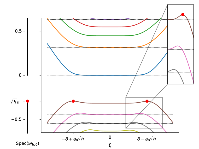
Figure 2. Dispersion curves for $h=0.05$

Let us describe some properties of the operators $(\mathscr{D}_{h,0,\xi})_{\xi}$. The associated dispersion curves are illustrated in Figure 2.

Proposition 2.3.

Let $h>0$. The following holds.

1. For $\xi\in\mathbb{R}$, the operator $\mathscr{D}_{h,0,\xi}$ is neither bounded from below nor from above, it is self-adjoint, inversible and has compact resolvent. Its eigenvalues are simple and denoted by

   $$\ldots\leqslant-\mu_{2}^{-}(\xi,h)\leqslant-\mu_{1}^{-}(\xi,h)<0<\mu_{1}^{+}(\xi,h)\leqslant\mu_{2}^{+}(\xi,h)\leqslant\ldots\,.$$

2. For $k\in\mathbb{N}\setminus\{0\}$, the map $\xi\mapsto\mu_{k}^{\pm}(\xi,h)$ is analytic and even.

The main tool in this study is the non-linear min-max characterization obtained in [3] adapted to our setting.

Proposition 2.4.

We have

$$\mu^{\pm}_{1}(\xi,h)=\min_{\psi\in H^{1}(I)\setminus\{0\}}\frac{h\|\psi\|^{2}_{\partial I}+\sqrt{h^{2}\|\psi\|^{4}_{\partial I}+4\|\psi\|^{2}\|(\pm h\partial_{t}+t+\xi)\psi\|^{2}}}{2\|\psi\|^{2}}\,.$$

Moreover, $\mu^{\pm}_{1}(\xi,h)$ is the smallest positive solution $\lambda$ of

$$\ell^{\pm}_{1}(\lambda,\xi,h)=0\,,$$

where $\ell^{\pm}_{1}(\lambda,\xi,h)$ is the lowest eigenvalue of the self-adjoint operator $\mathscr{L}_{\lambda,\xi,h}^{\pm}$ whose associated quadratic form is

$$\mathscr{Q}^{\pm}_{\lambda,\xi,h}(\psi)=\|(\pm h\partial_{t}+\xi+t)\psi\|^{2}+\lambda h\|\psi\|^{2}_{\partial I}-\lambda^{2}\|\psi\|^{2}\,,\quad\forall\psi\in H^{1}(I)\,.$$

In addition, we have for $\lambda>0$,

$$|\ell^{\pm}_{1}(\lambda,\xi,h)|\geqslant\lambda|\mu_{1}^{\pm}(\xi,h)-\lambda|\,.$$

2.2.1. Proof of the symmetry of the dispersion curves

To prove that the dispersion curves are even, note that $\Omega_{0}$ is left stable by the point symmetry around $0$. The covariance of the Dirac operator is expressed on the fibered operators in the following lemma ($i\sigma_{3}$ being the rotor associated with the symmetry).

Lemma 2.5.

Considering the unitary transformation $S:\psi\mapsto i\sigma_{3}\psi(-\cdot)$, we have, for all $\xi\in\mathbb{R}$, $S\mathrm{Dom}(\mathscr{D}_{h,0,\xi})=\mathrm{Dom}(\mathscr{D}_{h,0,\xi})$ and

$$S^{*}\mathscr{D}_{h,0,\xi}S=\mathscr{D}_{h,0,-\xi}\,.$$

In particular, we have

$$\mu^{\pm}_{k}(\xi,h)=\mu^{\pm}_{k}(-\xi,h)\,.$$

Remark 2.6.

Note that the charge conjugation for the bidimentionnal Dirac operator is $C\colon\psi\mapsto\sigma_{1}\overline{\psi}$. For the fibered ones, it reduces to a multiplication by $\sigma_{1}$ and to a change of sign for $\xi$. This leaves the domain $\mathrm{Dom}(\mathscr{D}_{h,0,\xi})$ stable. The operator $\mathscr{D}_{h,0,\xi}$ is transformed into $-\left((\xi-t)\sigma_{1}+\sigma_{2}D_{t}\right)$ (the magnetic field has opposite sign).

2.2.2. Some elements of the Proof of Points (i) and (ii) of Proposition 2.3

The proof follows classical steps as presented in [3, Proposition 4.2]. Let us recall why $\mathscr{D}_{h,0,\xi}$ is inversible. Since the spectrum is discrete, it is sufficient to consider the equation $\mathscr{D}_{h,0,\xi}\psi=0$. Let $\psi\in\ker(\mathscr{D}_{h,0,\xi})$. We have

$$(\xi-h\partial_{t}+t)\psi_{2}=0\,,\quad(\xi+h\partial_{t}+t)\psi_{1}=0\,.$$

Then,

$$\langle(\xi-h\partial_{t}+t)\psi_{2},\psi_{1}\rangle=0\,,$$

and, by integration by parts,

$$\langle(\xi-h\partial_{t}+t)\psi_{2},\psi_{1}\rangle=-h(\psi_{2}(\delta)\overline{\psi_{1}}(\delta)-\psi_{2}(-\delta)\overline{\psi_{1}}(-\delta))=0\,,$$

so that, using the boundary condition, $\psi_{1}(\pm\delta)=\psi_{2}(\pm\delta)=0$. Thus, $\psi_{1},\psi_{2}$ vanish at the boundary and solve first order linear ordinary differential equations, therefore $\psi=0$.

2.3. Study of $\mu^{+}_{1}(\xi,h)$

The following proposition presents some properties of the first positive dispersion curve.

Proposition 2.7.

1. For all $\xi$, we have $\mu^{+}_{1}(\xi,h)\leqslant\nu_{1}(\xi,h)$ , with

   $$\nu_{1}(\xi,h):=\frac{h(e^{-\frac{(\xi-\delta)^{2}}{h}}+e^{-\frac{(\xi+\delta)^{2}}{h}})}{\int_{-\delta}^{\delta}e^{-(\xi+t)^{2}/h}\mathrm{d}t}\,.$$

2. $\inf_{\xi\in\mathbb{R}}\nu_{1}(\xi,h)=\nu_{1}(0,h)=2\sqrt{\frac{h}{\pi}}e^{-\frac{\delta^{2}}{h}}(1+o_{h\to 0}(1))\,.$

3. For all $|\xi|>\delta$,

   $$\mu_{1}^{+}(\xi,h)\geqslant|\xi|-\delta-\frac{h}{|\xi|-\delta}\,.$$

4. For all $\xi$ such that $\mu_{1}^{+}(\xi,h)\leqslant\sqrt{h}e^{-\delta^{2}/h}$ we have

   $$\mu_{1}^{+}(\xi,h)\geqslant\nu_{1}(\xi,h)\left(1+o_{h\to 0}(1)\right)$$

   with $o_{h\to 0}(1)$ uniform in $\xi$.

Proposition 2.7 gathers the ingredient to characterize the positive part of the spectrum of $\mathscr{D}_{h,0}$ as stated in Theorem 1.3.

Corollary 2.8.

We have

$$\mathrm{sp}(\mathscr{D}_{h,0})\cap[0,+\infty[=[\lambda^{+}_{\rm ess}(h),+\infty[\,,$$

with $\lambda^{+}_{\rm ess}(h):=\inf_{\xi\in\mathbb{R}}\mu_{1}^{+}(\xi,h)=2\sqrt{\frac{h}{\pi}}e^{-\delta^{2}/h}(1+o_{h\to 0}(1))$.

Proof.

We have

$$\{\mu_{1}^{+}(\xi,h)\,,\xi\in\mathbb{R}\}\subset\mathrm{sp}(\mathscr{D}_{h,0})\cap[0,+\infty[\,,$$

and

$$\lambda^{+}_{\rm ess}(h)=\inf_{\xi\in\mathbb{R}}\mu_{1}^{+}(\xi,h)=\inf\mathrm{sp}(\mathscr{D}_{h,0})\cap[0,+\infty[\,.$$

By Point (c) of Proposition 2.7, we get that

$$\{\mu_{1}^{+}(\xi,h)\,,\xi\in\mathbb{R}\}=[\lambda^{+}_{\rm ess}(h),+\infty[\,.$$

By Points (a) and (b) of Proposition 2.7, we also have that

$$\lambda^{+}_{\rm ess}(h)\leqslant\mu_{1}^{+}(0,h)\leqslant 2\sqrt{\frac{h}{\pi}}e^{-\delta^{2}/h}(1+o_{h\to 0}(1))\,.$$

Now, let $(\xi_{h})$ such that for all $h$, $\lambda^{+}_{\rm ess}(h)\geqslant\mu_{1}^{+}(\xi_{h},h)(1+o_{h\to 0}(1))$. Points (b) and (d) ensure then that

$$\lambda^{+}_{\rm ess}(h)\geqslant\mu_{1}^{+}(\xi_{h},h)(1+o_{h\to 0}(1))\geqslant\nu_{1}(\xi_{h},h)(1+o_{h\to 0}(1))\geqslant\nu_{1}(0,h)(1+o_{h\to 0}(1))$$

and the conclusion follows. ∎

2.3.1. Proof of Point (a) and (b) of Proposition 2.7

By considering the function $u_{\xi}(t)=e^{-\frac{(\xi+t)^{2}}{2h}}$, Proposition 2.4 implies Point (a). To prove (b), remark that

$$\nu_{1}(\xi,h)=he^{-\delta^{2}/h}\frac{e^{2\xi\delta/h}+e^{-2\xi\delta/h}}{\int_{-\delta}^{\delta}e^{-2\xi t/h}e^{-t^{2}/h}\mathrm{d}t}\,,$$

and

$$\partial_{\xi}\nu_{1}(\xi,h)=\frac{2e^{-\delta^{2}/h}}{\left(\int_{-\delta}^{\delta}e^{-2\xi t/h}e^{-t^{2}/h}\mathrm{d}t\right)^{2}}\Big{[}(e^{2\xi\delta/h}-e^{-2\xi\delta/h})\int_{-\delta}^{\delta}\delta e^{-2\xi t/h}e^{-t^{2}/h}\mathrm{d}t\\ +(e^{2\xi\delta/h}+e^{-2\xi\delta/h})\int_{-\delta}^{\delta}te^{-2\xi t/h}e^{-t^{2}/h}\mathrm{d}t\Big{]}\,.$$

The quantity between the brackets equals

$$\int_{-\delta}^{\delta}(t+\delta)e^{(\delta-t)\xi/h}e^{-t^{2}/h}\mathrm{d}t+\int_{-\delta}^{\delta}(t-\delta)e^{-(\delta+t)\xi/h}e^{-t^{2}/h}\mathrm{d}t\,,$$

and also (by using $t\mapsto-t$ in the second integral)

$$\int_{-\delta}^{\delta}(t+\delta)e^{(\delta-t)\xi/h}e^{-t^{2}/h}\mathrm{d}t-\int_{-\delta}^{\delta}(t+\delta)e^{-(\delta-t)\xi/h}e^{-t^{2}/h}\mathrm{d}t\\ =2\int_{-\delta}^{\delta}(t+\delta)\sinh((\delta-t)\xi/h)e^{-t^{2}/h}\mathrm{d}t\,.$$

Thus,

$$\partial_{\xi}\nu_{1}(\xi,h)=\frac{4e^{-\delta^{2}/h}}{\left(\int_{-\delta}^{\delta}e^{-2\xi t/h}e^{-t^{2}/h}\mathrm{d}t\right)^{2}}\int_{-\delta}^{\delta}(t+\delta)\sinh((\delta-t)\xi/h)e^{-t^{2}/h}\mathrm{d}t\,,$$

which is positive when $\xi>0$. Therefore, the function $\xi\mapsto\nu_{1}(\xi,h)$ is even, increasing on $\mathbb{R}_{+}$ and Point (b) follows.

2.3.2. Proof of Point (c) of Proposition 2.7

We consider the case $\xi>\delta$. Let us use Proposition 2.4 and consider $\ell_{1}^{+}(\lambda,\xi,h)$ with $\lambda=\xi-\delta>0$. We have

$$\mathscr{Q}^{+}_{\lambda,\xi,h}(\psi)=\|h\partial_{t}\psi\|^{2}+\|(\xi+t)\psi\|^{2}+2h\mathrm{Re}\,\langle\partial_{t}\psi,(\xi+t)\psi\rangle+\lambda h\|\psi\|^{2}_{\partial I}-\lambda^{2}\|\psi\|^{2}\,,$$

and, by integration by parts,

$$\mathscr{Q}^{+}_{\lambda,\xi,h}(\psi)=\|h\partial_{t}\psi\|^{2}+\|(\xi+t)\psi\|^{2}-h\|\psi\|^{2}\\ +h(\xi+\delta)|\psi(\delta)|^{2}-h(\xi-\delta)|\psi(-\delta)|^{2}+\lambda h\|\psi\|^{2}_{\partial I}-\lambda^{2}\|\psi\|^{2}\,.$$

Since $\xi>\delta$ we have $\|(\xi+t)\psi\|^{2}\geqslant\lambda^{2}\|\psi\|^{2}$. We deduce that

$$\mathscr{Q}^{+}_{\lambda,\xi,h}(\psi)\geqslant-h\|\psi\|^{2}\,,$$

so that

$$\ell_{1}^{+}(\xi-\delta,\xi,h)\geqslant-h\,.$$

If $\ell_{1}^{+}(\xi-\delta,\xi,h)\geqslant 0$, then $\mu_{1}^{+}(\xi,h)\geqslant\xi-\delta$ (see Proposition 2.4). If $\ell_{1}^{+}(\xi-\delta,\xi,h)<0$, we get $|\ell_{1}^{+}(\xi-\delta,\xi,h)|\leqslant h$ so that

$$(\xi-\delta)|\mu^{+}_{1}(\xi,h)-(\xi-\delta)|\leqslant h\,.$$

When $\xi<-\delta$ we proceed similarly.

2.3.3. Proof of Point (d) of Proposition 2.7

Let us turn to lower bounds for $\mu_{1}^{+}(\cdot,h)$. By Point (a) and (b), there is $h_{0}>0$ such that for $h\in(0,h_{0})$,

$$\Xi_{h}:=\left\{\xi\geqslant 0:\mu_{1}^{+}(\xi,h)\leqslant\sqrt{h}e^{-\frac{\delta^{2}}{h}}\right\}\neq\emptyset\,.$$ (2.2)

Notation 2.9.

We consider on $L^{2}(I)$ the operator

$$d_{h,\xi}=-h\partial_{t}+\xi+t$$

with domain

$$\mathrm{Dom}(d_{h,\xi})=H^{1}_{0}(I)\,.$$

Its adjoint is

$$d^{*}_{h,\xi}=h\partial_{t}+\xi+t$$

with domain

$$\mathrm{Dom}(d_{h,\xi}^{*})=H^{1}(I).$$

We denote by $\Pi_{\xi}$ the orthogonal projection on $\mathrm{Ker}(d_{h,\xi}^{*})$, which is spanned by $t\mapsto e^{-(\xi+t)^{2}/2h}$.

Notation 2.10.

Let $\xi\in\mathbb{R}$. By Proposition 2.4, we consider $\psi_{\xi}\in H^{1}(I)$ such that $\|\psi_{\xi}\|=1$ and

$$\mu_{1}^{+}(\xi,h)=\frac{h}{2}\|\psi_{\xi}\|^{2}_{\partial I}+\frac{1}{2}\sqrt{h^{2}\|\psi_{\xi}\|^{4}_{\partial I}+4\|(h\partial_{t}+t+\xi)\psi_{\xi}\|^{2}}\,.$$

Lemma 2.11.

There exist $h_{0}>0$ and $C>0$ such that, for all $h\in(0,h_{0})$ and $\xi\in\Xi_{h}$,

$$\|\psi_{\xi}-\Pi_{\xi}\psi_{\xi}\|_{H^{1}(I)}\leqslant Ch^{-\frac{3}{2}}e^{-\delta^{2}/h}\,.$$

Proof.

For all $\xi\in\Xi_{h}$, we have

$$\|d_{h,\xi}^{*}(\psi_{\xi}-\Pi_{\xi}\psi_{\xi})\|=\|d_{h,\xi}^{*}\psi_{\xi}\|\leqslant\mu_{1}^{+}(\xi,h)\leqslant\sqrt{h}e^{-\frac{\delta^{2}}{h}}\,.$$

Since $d_{h,\xi}$ has closed range, we have $\psi_{\xi}-\Pi_{\xi}\psi_{\xi}\in\mathrm{Ker}(d_{h,\xi}^{*})^{\bot}=\mathrm{Ran}(d_{h,\xi})$. Let $\varphi_{\xi}\in H^{2}(I)\cap H_{0}^{1}(I)$ such that $d_{h,\xi}\varphi_{\xi}=\psi_{\xi}-\Pi_{\xi}\psi_{\xi}$. We consider the operator

$$\mathscr{L}_{h,\xi}^{+}=d_{h,\xi}^{*}d_{h,\xi}=-h^{2}\partial_{t}^{2}+(\xi+t)^{2}+h\,,$$

with domain $H^{2}(I)\cap H_{0}^{1}(I)$. We have $\|\mathscr{L}_{h,\xi}^{+}\varphi_{\xi}\|\leqslant h^{\frac{1}{2}}e^{-\frac{\delta^{2}}{h}}$. Note that, since $\varphi_{\xi}$ satisfies the Dirichlet boundary condition, we have

$$\|\mathscr{L}_{h,\xi}^{+}\varphi_{\xi}\|^{2}=\|h^{2}\partial_{t}^{2}\varphi_{\xi}\|^{2}+\|(\xi+t)^{2}\varphi_{\xi}\|^{2}+\|h\varphi_{\xi}\|^{2}+2h^{3}\|\partial_{t}\varphi_{\xi}\|^{2}+2h\|(\xi+t)\varphi_{\xi}\|^{2}\\ +2\mathrm{Re}\,\left\langle-h^{2}\partial_{t}^{2}\varphi_{\xi},(\xi+t)^{2}\varphi_{\xi}\right\rangle\,.$$

Moreover,

$$2\mathrm{Re}\,\left\langle-h^{2}\partial_{t}^{2}\varphi_{\xi},(\xi+t)^{2}\varphi_{\xi}\right\rangle=2h^{2}\mathrm{Re}\,\left\langle\partial_{t}\varphi_{\xi},\partial_{t}\left[(\xi+t)^{2}\varphi_{\xi}\right]\right\rangle$$

and

$$2h^{2}\mathrm{Re}\,\left\langle\partial_{t}\varphi_{\xi},\partial_{t}[(\xi+t)^{2}\varphi_{\xi}]\right\rangle =2h^{2}\|(\xi+t)\partial_{t}\varphi_{\xi}\|^{2}+4h^{2}\mathrm{Re}\,\left\langle\partial_{t}\varphi_{\xi},(\xi+t)\varphi_{\xi}\right\rangle$$

$$=2h^{2}\|(\xi+t)\partial_{t}\varphi_{\xi}\|^{2}-2h^{2}\|\varphi_{\xi}\|^{2}\,.$$

Therefore,

$$\|\mathscr{L}_{h,\xi}^{+}\varphi_{\xi}\|^{2}=\|h^{2}\partial_{t}^{2}\varphi_{\xi}\|^{2}+\|(\xi+t)^{2}\varphi_{\xi}\|^{2}+h^{2}\|\varphi_{\xi}\|^{2}+2h^{3}\|\partial_{t}\varphi_{\xi}\|^{2}+2h\|(\xi+t)\varphi_{\xi}\|^{2}\\ +2h^{2}\|(\xi+t)\partial_{t}\varphi_{\xi}\|^{2}-2h^{2}\|\varphi_{\xi}\|^{2}\,.$$

Thus,

$$\|\mathscr{L}_{h,\xi}^{+}\varphi_{\xi}\|^{2}=\|h^{2}\partial_{t}^{2}\varphi_{\xi}\|^{2}+\|(\xi+t)^{2}\varphi_{\xi}\|^{2}+h^{2}\|\varphi_{\xi}\|^{2}+2h^{2}\|(\xi+t)\partial_{t}\varphi_{\xi}\|^{2}\\ +2h\|(h\partial_{t}+\xi+t)\varphi_{\xi}\|^{2}\,.$$ (2.3)

and in particular

$$h^{4}\|\partial_{t}^{2}\varphi_{\xi}\|^{2}+h^{2}\|\varphi_{\xi}\|^{2}\leqslant(h^{1/2}e^{-\frac{\delta^{2}}{h}})^{2}\,.$$

Since $\varphi_{\xi}\in H^{2}(I)\cap H^{1}_{0}(I)$, we get

$$\|\varphi_{\xi}\|^{2}_{H^{2}(I)}\leqslant Ch^{-3}e^{-\frac{2\delta^{2}}{h}}\,.$$

Then, we have

$$\begin{split}\|d_{h,\xi}\varphi_{\xi}\|_{H^{1}(I)}&=\|(-h\partial_{t}+\xi+t)\varphi_{\xi}\|_{H^{1}(I)}\\ &\leqslant C\left(h\|\partial_{t}\varphi_{\xi}\|_{H^{1}}+\|(\xi+t)\varphi_{\xi}\|_{H^{1}}\right)\\ &\leqslant C\left(\|\varphi_{\xi}\|_{H^{2}(I)}+\|(\xi+t)\varphi_{\xi}\|+\|(\xi+t)\partial_{t}\varphi_{\xi}\|\right)\\ &\leqslant\tilde{C}h^{-\frac{3}{2}}e^{-\delta^{2}/h}\,,\end{split}$$

where we used (2.3) and the Cauchy-Schwarz inequality. ∎

Now we can prove Point (d). We have

$$\mu_{1}^{+}(\xi,h)\geqslant h\|\psi_{\xi}\|^{2}_{\partial I}\,.$$

By Lemma 2.11 and a usual trace theorem, considering $h$ small enough and $\xi\in\Xi_{h}$, we get

$$\|\psi_{\xi}-\Pi_{\xi}\psi_{\xi}\|+\|\psi_{\xi}-\Pi_{\xi}\psi_{\xi}\|_{\partial I}\leqslant Ch^{-\frac{3}{2}}e^{-\delta^{2}/h}\,,$$

so

$$\|\psi_{\xi}\|_{\partial I}^{2}=\frac{\|\Pi_{\xi}\psi_{\xi}\|_{\partial I}^{2}}{\|\Pi_{\xi}\psi_{\xi}\|^{2}}\left(1+o_{h\to 0}(1)\right).$$

Finally,

$$\frac{\|\Pi_{\xi}\psi_{\xi}\|_{\partial I}^{2}}{\|\Pi_{\xi}\psi_{\xi}\|^{2}}=\nu_{1}(\xi,h),$$

and the conclusion follows.

2.4. Study of $\mu^{-}_{1}(\xi,h)$

In this section, we continue the proof of Theorem 1.3 by establishing the estimate of $\lambda^{-}_{\mathrm{ess}}(h)$.

Proposition 2.12.

We have

1. There exists $C>0$ such that for all $|\xi|>\delta$,

   $$\mu_{1}^{-}(\xi,h)\geqslant|\xi|-\delta-\frac{C}{|\xi|-\delta}\,.$$

2. There exists $C>0$ such that for all $\xi$,

   $$\mu_{1}^{-}(\xi,h)\geqslant a_{0}\sqrt{h}-Ch^{3/2}\,.$$

   with $C$ independent of $\xi,h$.

3. We have

   $$\mu^{-}_{1}(\delta-\sqrt{h}a_{0},h)\leqslant a_{0}\sqrt{h}+\mathscr{O}(h^{\infty})\,.$$

This proposition 2.12 allows us to study the negative part of the spectrum of $\mathscr{D}_{h,0}$ as stated in Theorem 1.3.

Corollary 2.13.

We have

$$\mathrm{sp}(\mathscr{D}_{h,0})\cap]-\infty,0]=(-\infty,-\lambda^{-}_{\rm ess}(h)]\,,$$

with $\lambda^{-}_{\rm ess}(h):=\inf_{\xi\in\mathbb{R}}\mu_{1}^{-}(\xi,h)=\sqrt{h}a_{0}+\mathscr{O}(h^{3/2})$.

2.4.1. Proof of Point (a) of Proposition 2.12

As in Section 2.3.2, we consider the case $\xi>\delta$ and take $\lambda=\xi-\delta$. We have, for all $\psi\in H^{1}(I)$,

$$\mathscr{Q}^{-}_{\lambda,\xi,h}(\psi)=\|h\partial_{t}\psi\|^{2}+\|(\xi+t)\psi\|^{2}+h\|\psi\|^{2}\\ -h(\xi+\delta)|\psi(\delta)|^{2}+h(\xi-\delta)|\psi(-\delta)|^{2}+\lambda h\|\psi\|^{2}_{\partial I}-\lambda^{2}\|\psi\|^{2}\,.$$

Since $\xi>\delta$, we have for $t\in(-\delta,\delta)$, $(\xi+t)^{2}\geqslant(\xi-\delta)^{2}=\lambda^{2}$. Moreover,

$$-h(\xi+\delta)|\psi(\delta)|^{2}+h(\xi-\delta)|\psi(-\delta)|^{2}+\lambda h\|\psi\|^{2}_{\partial I}=-2h\delta|\psi(\delta)|^{2}+2h(\xi-\delta)|\psi(-\delta)|^{2}\,,$$

so that

$$\mathscr{Q}^{-}_{\lambda,\xi,h}(\psi)\geqslant\|h\partial_{t}\psi\|^{2}+h\|\psi\|^{2}-2h\delta|\psi(\delta)|^{2}\,.$$

By Sobolev embedding, we recall that there exists $C>0$ such that, for all $\epsilon>0$,

$$\|\psi\|^{2}_{L^{\infty}(I)}\leqslant\epsilon\|\partial_{t}\psi\|^{2}+C\epsilon^{-1}\|\psi\|^{2}\,.$$

Thus, with $\epsilon=h(2\delta)^{-1}$, we deduce that

$$\mathscr{Q}^{-}_{\lambda,\xi,h}(\psi)\geqslant-4C\delta^{2}\|\psi\|^{2}\,.$$

Therefore, by the min-max theorem,

$$\ell_{1}^{-}(\lambda,\xi,h)\geqslant-4C\delta^{2}\,.$$

By Proposition 2.4, if $\ell_{1}^{-}(\lambda,\xi,h)\geqslant 0$, then $\mu_{1}^{-}(\xi,h)\geqslant\lambda=\xi-\delta$. If $\ell_{1}^{-}(\lambda,\xi,h)\leqslant 0$, then $|\ell_{1}^{-}(\lambda,\xi,h)|\leqslant 4C\delta^{2}$. Thus,

$$\mu_{1}^{-}(\xi,h)\geqslant\xi-\delta-4C\delta^{2}(\xi-\delta)^{-1}\,.$$

2.4.2. Proof of Point (b) of Proposition 2.12

Let us denote for $u\in\{v\in H^{1}(\mathbb{R})\,,tv(t)\in L^{2}(\mathbb{R})\}$,

$$\begin{split}\mathscr{Q}^{-}_{\lambda,\xi,\mathbb{R}}(u):=\|(-\partial_{t}+\xi+t)u\|^{2}_{L^{2}(\mathbb{R})}+\lambda|u(0)|^{2}-\lambda^{2}\|u\|^{2}_{L^{2}(\mathbb{R})}\,,\end{split}$$

and $u\in\{v\in H^{1}(\mathbb{R}_{+})\,,tv(t)\in L^{2}(\mathbb{R}_{+})\}$,

$$\begin{split}\mathscr{Q}^{-}_{\lambda,\xi,\mathbb{R}_{+}}(u):=\|(-\partial_{t}+\xi+t)u\|^{2}_{L^{2}(\mathbb{R}_{+})}+\lambda|u(0)|^{2}-\lambda^{2}\|u\|^{2}_{L^{2}(\mathbb{R}_{+})}\,.\end{split}$$

Let $(\chi_{1},\chi_{2},\chi_{3})$ be a partition of the unity of $[-\delta,\delta]$ such that $\mathrm{supp}(\chi_{1})\subset[-\delta,-\delta/3]$, $\mathrm{supp}(\chi_{2})\subset[-2\delta/3,2\delta/3]$, $\mathrm{supp}(\chi_{3})\subset[\delta/3,\delta]$,

$$\chi_{1}^{2}+\chi^{2}_{2}+\chi_{3}^{2}=1\;\;\text{and}\;\;|\partial_{t}\chi_{1}|^{2}+|\partial_{t}\chi_{2}|^{2}+|\partial_{t}\chi_{3}|^{2}\leqslant C\,.$$

From the localization formula, we have

$$\begin{split}\|(-h\partial_{t}+\xi+t)\psi\|^{2}&=\sum_{j=1}^{3}\left(\|(-h\partial_{t}+\xi+t)(\chi_{j}\psi)\|^{2}-\|h(\partial_{t}\chi_{j})\psi\|^{2}\right)\\ &\geqslant-Ch^{2}\|\psi\|^{2}+\sum_{j=1}^{3}\|(-h\partial_{t}+\xi+t)(\chi_{j}\psi)\|^{2}\,,\end{split}$$

so that

$$\mathscr{Q}^{-}_{\lambda,\xi,h}(\psi)\geqslant-Ch^{2}\|\psi\|^{2}+\sum_{j=1}^{3}\mathscr{Q}^{-}_{\lambda,\xi,h}(\chi_{i}\psi).$$

We denote $v_{1}\colon s\in\mathbb{R}_{+}\mapsto(\chi_{1}\psi)(s\sqrt{h}-\delta)$, $v_{2}\colon s\in\mathbb{R}\mapsto(\chi_{2}\psi)(s\sqrt{h})$ and $v_{3}\colon s\in\mathbb{R}_{+}\mapsto(\chi_{3}\psi)(\delta-s\sqrt{h})$ so that

$$\begin{split}&\mathscr{Q}^{-}_{\lambda,\xi,h}(\chi_{1}\psi)=h^{3/2}\mathscr{Q}^{-}_{\frac{\lambda}{\sqrt{h}},\frac{\xi-\delta}{\sqrt{h}},\mathbb{R}_{+}}(v_{1})\,,\\ &\mathscr{Q}^{-}_{\lambda,\xi,h}(\chi_{2}\psi)=h^{3/2}\mathscr{Q}^{-}_{\frac{\lambda}{\sqrt{h}},\frac{\xi}{\sqrt{h}},\mathbb{R}}(v_{2})\,,\\ &\mathscr{Q}^{-}_{\lambda,\xi,h}(\chi_{3}\psi)=h^{3/2}\mathscr{Q}^{-}_{\frac{\lambda}{\sqrt{h}},-\frac{\xi+\delta}{\sqrt{h}},\mathbb{R}_{+}}(v_{3})\,.\end{split}$$

Now, fix $\lambda=a_{0}\sqrt{h}$. By [3, Propositions 4.12, 4.15], the map $\xi\mapsto\inf_{v\neq 0}\frac{1}{\|v\|^{2}}\mathscr{Q}^{-}_{a_{0},\xi,\mathbb{R}_{+}}(v)$ is non-negative and has a unique non-degenerate minimum at $\xi=-a_{0}$, which is zero. By [3, Theorem 4.3], the map $\xi\mapsto\inf_{v\neq 0}\frac{1}{\|v\|^{2}}\mathscr{Q}^{-}_{a_{0},\xi,\mathbb{R}}(v)$ is constant equal to $2-a_{0}^{2}$. Therefore, there exists $c_{0}>0$ such that

$$\sum_{j=1}^{3}\mathscr{Q}^{-}_{\lambda,\xi,h}(\chi_{i}\psi)\geqslant h^{3/2}c_{0}\min\left(1,\left|\frac{\xi-\delta}{\sqrt{h}}+a_{0}\right|^{2},\left|-\frac{\xi+\delta}{\sqrt{h}}+a_{0}\right|^{2}\right)\|\psi\|^{2}\,.$$

We obtain then that

$$\ell^{-}_{1}(\sqrt{h}a_{0},\xi,h)\geqslant h^{3/2}c_{0}\min\left(1,\left|\frac{\xi-\delta}{\sqrt{h}}+a_{0}\right|^{2},\left|-\frac{\xi+\delta}{\sqrt{h}}+a_{0}\right|^{2}\right)-Ch^{2}\,.$$ (2.4)

By Proposition 2.4, if $\ell^{-}_{1}(\sqrt{h}a_{0},\xi,h)\geqslant 0$, then $\mu^{-}_{1}(\xi,h)\geqslant\sqrt{h}a_{0}$. If $\ell^{-}_{1}(\sqrt{h}a_{0},\xi,h)\leqslant 0$, then $\sqrt{h}a_{0}-\mu^{-}_{1}(\xi,h)\geqslant 0$ and

$$\sqrt{h}a_{0}(\sqrt{h}a_{0}-\mu^{-}_{1}(\xi,h))\leqslant|\ell^{-}_{1}(\sqrt{h}a_{0},\xi,h)|\leqslant Ch^{2}\,,$$

so

$$\mu^{-}_{1}(\xi,h)\geqslant\sqrt{h}a_{0}-Ch^{3/2}\,.$$

Note that (2.4) suggests that the minima of $\xi\mapsto\mu^{-}_{1}(\xi,h)$ occur near $\xi=\delta-\sqrt{h}a_{0}$ and $\xi=-\delta+\sqrt{h}a_{0}$ (see Figure 2). However, we leave the investigation of a more precise determination of the minima’s location as an open question.

2.4.3. Proof of Point (c) of Proposition 2.12

Let us focus on upper bounds on $\mu^{-}_{1}$. Following the notations of [3, Section 4.4], we denote by $u_{a_{0},-a_{0}}$ the normalized ground state of $\mathscr{Q}^{-}_{a_{0},-a_{0},\mathbb{R}_{+}}$. Its energy is $0$. Let $v\colon t\in(-\delta,\delta)\mapsto u_{a_{0},-a_{0}}\left(\frac{t+\delta}{\sqrt{h}}\right)$. Since $u_{a_{0},-a_{0}}$ belongs to the Schwartz class, the rescaling performed in the previous section ensures that

$$\mathscr{Q}^{-}_{\sqrt{h}a_{0},\delta-\sqrt{h}a_{0},h}(v)=h^{3/2}\mathscr{Q}^{-}_{a_{0},-a_{0},\mathbb{R}_{+}}(u_{a_{0},-a_{0}})+\mathscr{O}(h^{\infty})=\mathscr{O}(h^{\infty})\,,$$

so that

$$\ell^{-}_{1}(\sqrt{h}a_{0},\delta-\sqrt{h}a_{0},h)\leqslant\mathscr{O}(h^{\infty})\,.$$

By Proposition 2.4, if $\ell^{-}_{1}(\sqrt{h}a_{0},\delta-\sqrt{h}a_{0},h)\geqslant 0$, then $\mu^{-}_{1}(\delta-\sqrt{h}a_{0},h)\geqslant\sqrt{h}a_{0}$ and

$$\sqrt{h}a_{0}\left(\mu^{-}_{1}(\delta-\sqrt{h}a_{0},h)-\sqrt{h}a_{0}\right)\leqslant\ell^{-}_{1}(\sqrt{h}a_{0},\delta-\sqrt{h}a_{0},h)\leqslant\mathscr{O}(h^{\infty})\,,$$

so that

$$\mu^{-}_{1}(\delta-\sqrt{h}a_{0},h)\leqslant\sqrt{h}a_{0}+\mathscr{O}(h^{\infty})\,.$$

If $\ell^{-}_{1}(\sqrt{h}a_{0},\delta-\sqrt{h}a_{0},h)\leqslant 0$, then $\mu^{-}_{1}(\delta-\sqrt{h}a_{0},h)\leqslant\sqrt{h}a_{0}$ .

3. Estimates of the discrete spectrum

3.1. Upper bound of Point (i) of Theorem 1.6

Let $k\in\mathbb{N}^{*}$ be fixed in this section.

Notation 3.1.

1. We denote by $\{v_{0},\dots,v_{k-1}\}\subset\mathscr{H}^{2}(\Omega)$ a $k$-dimensional family of Hardy functions satisfying for $j,l\in\{0,\dots,k-1\}$, $v_{l}^{(j)}(z_{\rm min})=\delta_{jl}$, $\delta_{jl}$ being the Kronecker delta. We assume moreover that $v_{k-1}$ is the unique minimizer of $d^{k}_{\mathscr{H}}={\rm dist}_{\mathscr{H}^{2}(\Omega)}(0,\mathbb{X}_{k})$ where $\mathbb{X}_{k}$ is defined before Theorem 1.6.

2. The familly $(P_{n})_{n\in\mathbb{N}}$ is the $N_{\mathscr{B}}$-orthogonal family obtained after a Gram-Schmidt process on $(1,Z,\dots,Z^{n},\dots)$ and normalized by $P_{n}^{(n)}(0)=b_{n,n}=1$ in $P_{n}(Z)=\sum_{j=0}^{n}\frac{b_{n,j}}{j!}Z^{j}$.

3. For $n\in\{0,\dots,k-1\}$, we define $w_{n}=\sum_{j=0}^{n}b_{n,j}h^{\frac{n-j}{2}}v_{j}$.

4. $\mathrm{Tayl}(w)$ is the polynomial part of the Taylor expansion of degree $k-1$ of the function $w$ at $z_{\rm min}$ :

   $$\mathrm{Tayl}(w)(z)=\sum_{l=0}^{k-1}\frac{w^{(l)}(z_{\rm min})}{l!}\left(z-z_{\rm min}\right)^{l}\,.$$

Lemma 3.2.

We have for $n\in\{0,\dots k-1\}$,

$$\mathrm{Tayl}(w_{n})\left(z_{\rm min}+\sqrt{h}z\right)=h^{\frac{n}{2}}P_{n}(z)\,.$$

Proof.

Let $l,n\in\{0,\dots k-1\}$, we have

$$w_{n}^{(l)}(z_{\rm min})=\sum_{j=0}^{n}b_{n,j}h^{\frac{n-j}{2}}v_{j}^{(l)}(z_{\rm min})=\sum_{j=0}^{n}b_{n,j}h^{\frac{n-j}{2}}\delta_{lj}=b_{n,l}h^{\frac{n-l}{2}}\,,$$

and

$$\mathrm{Tayl}(w_{n})\left(z_{\rm min}+\sqrt{h}z\right)=\sum_{l=0}^{k-1}\frac{w_{n}^{(l)}(z_{\rm min})}{l!}\left(\sqrt{h}z\right)^{l}=h^{\frac{n}{2}}P_{n}(z)\,.$$

∎

Lemma 3.3.

Let $c_{0},\dots,c_{k-1}\in\mathbb{C}$ and $w=\sum_{n=0}^{k-1}c_{n}w_{n}$. We have

$$\int_{\Omega}\left|\sum_{n=0}^{k-1}c_{n}w_{n}\right|^{2}e^{-2(\phi-\phi_{\rm min})/h}{\rm d}x\geqslant(1+o(1))h\sum_{j=0}^{k-1}|h^{j/2}c_{j}|^{2}N_{\mathscr{B}}\left(P_{j}\right)^{2}\,.$$

Proof.

Let $\eta\in(1/3,1/2)$. By Taylor’s formula, there exists $C>0$ such that for $x\in D(x_{\rm min},h^{\eta})$

$$\begin{split}\phi(x)-\phi_{\rm min}\leqslant\frac{1}{2}{\rm Hess}_{\rm min}\phi(x-x_{\rm min},x-x_{\rm min})+h^{3\eta}C\end{split}$$

and with $x=x_{\rm min}+\sqrt{h}y$,

$$\begin{split}&\int_{\Omega}|w|^{2}e^{-2(\phi-\phi_{\rm min})/h}{\rm d}x\geqslant\int_{B(x_{\rm min},h^{\eta})}|w|^{2}e^{-2(\phi-\phi_{\rm min})/h}{\rm d}x\\ &\geqslant e^{-2Ch^{3\eta-1}}\int_{B(x_{\rm min},h^{\eta})}|w|^{2}e^{-{\rm Hess}_{\rm min}\phi(x-x_{\rm min},x-x_{\rm min})/h}{\rm d}x\\ &\geqslant(1+o(1))\int_{B(x_{\rm min},h^{\eta})}|w|^{2}e^{-{\rm Hess}_{\rm min}\phi(x-x_{\rm min},x-x_{\rm min})/h}{\rm d}x\\ &\geqslant(1+o(1))h\int_{B(0,h^{\eta-1/2})}|w(x_{\rm min}+\sqrt{h}y)|^{2}e^{-{\rm Hess}_{\rm min}\phi(y,y)}{\rm d}y\,.\end{split}$$

By Lemma 3.2, we have for $y\in D(0,h^{\eta-1/2})$,

$$|w_{j}(x_{\rm min}+\sqrt{h}y)-h^{j/2}P_{j}(y)|\leqslant C(\sqrt{h}|y|)^{k}\,,$$

Thus we have

$$w(x_{\rm min}+\sqrt{h}y)={\mathrm{Tayl}}(w)(x_{\rm min}+\sqrt{h}y)+R_{h,c}(y)\,,$$

with

$$|R_{h,c}(y)|\leqslant C|y\sqrt{h}|^{k}\sum_{j=0}^{k-1}|c_{j}|\,.$$

By Young’s inequality, we have for $\varepsilon=h^{1/4}>0$, $\tilde{c}=(\tilde{c}_{j})_{j}=(h^{j/2}c_{j})_{j}$,

$$\begin{split}&h\int_{D(0,h^{\eta-1/2})}|w(x_{\rm min}+\sqrt{h}y)|^{2}e^{-{\rm Hess}_{\rm min}\phi(y,y)}{\rm d}y\\ &\geqslant(1-\varepsilon)h\int_{D(0,h^{\eta-1/2})}|{\rm Tayl}(w)(x_{\rm min}+\sqrt{h}y)|^{2}e^{-{\rm Hess}_{\rm min}\phi(y,y)}{\rm d}y\\ &\quad-\varepsilon^{-1}h\int_{D(0,h^{\eta-1/2})}|R_{h,c}(y)|^{2}e^{-{\rm Hess}_{\rm min}\phi(y,y)}{\rm d}y\\ &\geqslant(1-\varepsilon)h\int_{D(0,h^{\eta-1/2})}|\sum_{j=0}^{k-1}\tilde{c}_{j}P_{j}(y)|^{2}e^{-{\rm Hess}_{\rm min}\phi(y,y)}{\rm d}y-\varepsilon^{-1}h^{3/2}C\|\tilde{c}\|_{2}^{2}\\ &\geqslant(1+o(1))hN_{\mathscr{B}}\left(\sum_{j=0}^{k-1}\tilde{c}_{j}P_{j}(y)\right)^{2}+o(h)\|\tilde{c}\|_{2}^{2}\end{split}$$

By the orthogonality of the $(P_{j})$ family, we get

$$\begin{split}N_{\mathscr{B}}\left(\sum_{j=0}^{k-1}\tilde{c}_{j}P_{j}(y)\right)^{2}=\sum_{j=0}^{k-1}|\tilde{c}_{j}|^{2}N_{\mathscr{B}}\left(P_{j}\right)^{2}\end{split}$$

and the equivalence of the norms in finite dimensions ensures

$$h\int_{D(0,h^{\eta-1/2})}|w(x_{\rm min}+\sqrt{h}y)|^{2}e^{-{\rm Hess}_{\rm min}\phi(y,y)}{\rm d}y\geqslant(1+o(1))h\sum_{j=0}^{k-1}|\tilde{c}_{j}|^{2}N_{\mathscr{B}}\left(P_{j}\right)^{2}\,.$$

∎

Lemma 3.4.

Let $c_{0},\dots,c_{k-1}\in\mathbb{C}$. We have

$$\begin{split}\sqrt{h}\|w\|_{\mathscr{H}^{2}(\Omega)}\leqslant\sqrt{h}(1+o(1))\sum_{j=0}^{k-1}|c_{j}|\|v_{j}\|_{\mathscr{H}^{2}(\Omega)}\,.\end{split}$$

Proof.

Let $w=\sum_{n=0}^{k-1}c_{n}w_{n}$. By the triangle inequality and the definition of $(w_{n})$, we have

$$\begin{split}\sqrt{h}\|w\|_{\mathscr{H}^{2}(\Omega)}&\leqslant\sqrt{h}\sum_{j=0}^{k-1}|c_{j}|\|w_{j}\|_{\mathscr{H}^{2}(\Omega)}\leqslant\sqrt{h}(1+o(1))\sum_{j=0}^{k-1}|c_{j}|\|v_{j}\|_{\mathscr{H}^{2}(\Omega)}\,,\end{split}$$

∎

Lemma 3.5.

We have,

$$\begin{split}\sup_{c\in\mathbb{C}^{k}\setminus\{0\}}\frac{h\left(\sum_{j=0}^{k-1}|c_{j}|\|v_{j}\|_{\mathscr{H}^{2}(\Omega)}\right)^{2}}{h\sum_{j=0}^{k-1}|h^{j/2}c_{j}|^{2}N_{\mathscr{B}}\left(P_{j}\right)^{2}}=(1+o(1))h^{(1-k)}\left(\frac{d^{k}_{\mathscr{H}}}{d^{k}_{\mathscr{B}}}\right)^{2}\,.\end{split}$$

Proof.

Considering $c=(0,\dots,0,1)$ we obtain

$$\begin{split}\sup_{c\in\mathbb{C}^{k}\setminus\{0\}}\frac{h\left(\sum_{j=0}^{k-1}|c_{j}|\|v_{j}\|_{\mathscr{H}^{2}(\Omega)}\right)^{2}}{h\sum_{j=0}^{k-1}|h^{j/2}c_{j}|^{2}N_{\mathscr{B}}\left(P_{j}\right)^{2}}\geqslant\frac{h^{(1-k)}\|v_{k-1}\|_{\mathscr{H}^{2}(\Omega)}^{2}}{N_{\mathscr{B}}\left(P_{k-1}\right)^{2}}\,.\end{split}$$

Conversely, for $c=(c_{0},\dots,c_{k-1})\in\mathbb{C}\setminus\{0\}$ we have

$$\begin{split}&\frac{\sum_{j=0}^{k-1}|c_{j}|\|v_{j}\|_{\mathscr{H}^{2}(\Omega)}}{\sqrt{\sum_{j=0}^{k-1}|h^{j/2}c_{j}|^{2}N_{\mathscr{B}}\left(P_{j}\right)^{2}}}=\frac{|c_{k-1}|\|v_{k-1}\|_{\mathscr{H}^{2}(\Omega)}+\sum_{j=0}^{k-2}|c_{j}|\|v_{j}\|_{\mathscr{H}^{2}(\Omega)}}{\sqrt{\sum_{j=0}^{k-1}|h^{j/2}c_{j}|^{2}N_{\mathscr{B}}\left(P_{j}\right)^{2}}}\\ &\leqslant\sqrt{\frac{h^{(1-k)}\|v_{k-1}\|_{\mathscr{H}^{2}(\Omega)}^{2}}{N_{\mathscr{B}}\left(P_{k-1}\right)^{2}}}+h^{(2-k)/2}\sup_{c\in\mathbb{C}^{k-1}}\frac{\sum_{j=0}^{k-2}|c_{j}|\|v_{j}\|_{\mathscr{H}^{2}(\Omega)}}{\sqrt{\sum_{j=0}^{k-2}|c_{j}|^{2}N_{\mathscr{B}}\left(P_{j}\right)^{2}}}\,.\end{split}$$

Note now that $\|v_{k-1}\|_{\mathscr{H}^{2}(\Omega)}=d^{k}_{\mathscr{H}}$ and $N_{\mathscr{B}}\left(P_{k-1}\right)=d^{k}_{\mathscr{B}}$. The result follows. ∎

The upper bound in Point (i) of Theorem 1.6 follow from Lemmas 3.3, 3.4 and 3.5.

3.2. Lower bound of Point (i) of Theorem 1.6

3.2.1. Preliminaries

The proof of the lower bound closely follows that presented in [3, Section 3.1.2]. A notable difference is that polynomials do not belong to the Hardy space $\mathscr{H}^{2}(\Omega)$. This is addressed through the introduction of the Hardy-Taylor expansion described below. Let $k\in\mathbb{N}^{*}$ be fixed in this section.

Notation 3.6.

1. For $l\in\{0,\dots,k-1\}$, we define

   $$\mathbb{X}_{k,l}=\{u\in\mathscr{H}^{2}(\Omega):\forall j\in\{0,\dots,k-1\},\;u^{(j)}(z_{\min})=\delta_{jl}\}.$$

   Then we denote by $v_{l}\in\mathbb{X}_{k,l}\subset\mathscr{H}^{2}(\Omega)$ the unique minimizer of $\mathrm{dist}_{\mathscr{H}^{2}(\Omega)}(0,\mathbb{X}_{k,l})$. Note that $\mathbb{X}_{k,k-1}=\mathbb{X}_{k}$ as defined in Point (i) of Theorem 1.6, ensuring that the notation for $v_{k}$ is consistent with that introduced in Notation 3.1.

2. We denote by $\mathrm{Tayl}_{\mathscr{H}^{2}(\Omega)}(w)$ the Hardy - Taylor expansion of degree $k-1$ of the function $w\in\mathscr{H}^{2}(\Omega)$ at $z_{\rm min}$ :

   $$\mathrm{Tayl}_{\mathscr{H}^{2}(\Omega)}(w)=\sum_{l=0}^{k-1}w^{(l)}(z_{\rm min})v_{l}\in\mathscr{H}^{2}(\Omega)\,.$$

3. We denote by $\mathscr{W}_{k}(h)\subset\mathscr{H}^{2}(\Omega)$ a subspace such that $\dim\mathscr{W}_{k}(h)=k$ and

   $$\sup_{w\in\mathscr{W}_{k}(h)\setminus\{0\}}\frac{h\|w\|^{2}_{\mathscr{H}^{2}(\Omega)}}{\|e^{-\phi/h}w\|^{2}}\leqslant\lambda^{\mathrm{eff}}_{k}(h)(1+o(1))\,.$$ (3.1)

Let us clarify the relationship between the Taylor expansion and the Hardy-Taylor expansion as defined in Notations 3.1 and 3.6 and prove a notable property of $\mathrm{Tayl}_{\mathscr{H}^{2}(\Omega)}$.

Lemma 3.7.

The following assertions hold:

1. The operator

   $$\mathrm{Tayl}_{\mathscr{H}^{2}(\Omega)}\colon\mathscr{H}^{2}(\Omega)\to\mathscr{H}^{2}(\Omega)$$

   is the $\mathscr{H}^{2}(\Omega)$-orthogonal projection onto the orthogonal of

   $$\widetilde{\mathbb{X}}_{k+1}=\{u\in\mathscr{H}^{2}(\Omega):\forall j\in\{0,\dots,k\},\;u^{(j)}(z_{\min})=0\}.$$

2. For any $w\in\mathscr{H}^{2}(\Omega)$, the following identity holds:

   $$\mathrm{Tayl}\left(w-\mathrm{Tayl}_{\mathscr{H}^{2}(\Omega)}(w)\right)=0\,.$$

Proof.

Let us begin with Point (ii):

$$\begin{split}\mathrm{Tayl}\left(\mathrm{Tayl}_{\mathscr{H}^{2}(\Omega)}(w)\right)(z)&=\sum_{l=0}^{k-1}w^{(l)}(z_{\rm min})\mathrm{Tayl}(v_{l})(z)=\sum_{l=0}^{k-1}\frac{w^{(l)}(z_{\rm min})}{l!}(z-z_{\rm min})^{l}\\ &=\mathrm{Tayl}(w)(z)\,.\end{split}$$

We now prove Point (i). Note that, by the Cauchy formula estimation from Point (iii) of Proposition A.12, $\widetilde{\mathbb{X}}_{k+1}$ and $(\mathbb{X}_{k,l})_{0\leqslant l\leqslant k-1}$ are (non empty) closed subspaces so that the orthogonal projection is indeed well-defined. Let $0\leqslant l\leqslant k-1$ and $u\in\widetilde{\mathbb{X}}_{k+1}$, then $u+v_{l}\in\mathbb{X}_{k,l}$. Since $v_{l}$ is the orthogonal projection of $0$ onto $\mathbb{X}_{k,l}$, we get

$$0=\langle v_{l},(u+v_{l})-v_{l}\rangle_{\mathscr{H}^{2}(\Omega)}=\langle v_{l},u\rangle_{\mathscr{H}^{2}(\Omega)}\,,$$

and $v_{l}\in(\widetilde{\mathbb{X}}_{k+1})^{\perp}$. This proves that

$${\rm span}(v_{0},\dots,v_{k-1})\subset(\widetilde{\mathbb{X}}_{k+1})^{\perp}\,.$$

Assume now that $u\in(\widetilde{\mathbb{X}}_{k+1})^{\perp}\cap({\rm span}(v_{0},\dots,v_{k-1}))^{\perp}$. Then, $u-\mathrm{Tayl}_{\mathscr{H}^{2}(\Omega)}(u)\in\widetilde{\mathbb{X}}_{k+1}$ so that

$$0=\langle u,u-\mathrm{Tayl}_{\mathscr{H}^{2}(\Omega)}(u)\rangle_{\mathscr{H}^{2}(\Omega)}=\|u\|^{2}_{\mathscr{H}^{2}(\Omega)}\,.$$

We proved that

$${\rm span}(v_{0},\dots,v_{k-1})=(\widetilde{\mathbb{X}}_{k+1})^{\perp}\,.$$ (3.2)

Finally, note that

$$\mathrm{Tayl}_{\mathscr{H}^{2}(\Omega)}(v)=\begin{cases}v&\text{ if }v\in{\rm span}(v_{0},\dots,v_{k-1})\,,\\ 0&\text{ if }v\in\widetilde{\mathbb{X}}_{k+1}\,.\end{cases}$$ (3.3)

We conclude from (3.2) and (3.3) that $\mathrm{Tayl}_{\mathscr{H}^{2}(\Omega)}$ is the orthogonal projection onto $(\widetilde{\mathbb{X}}_{k+1})^{\perp}$ and Point (i) follows.

Remark that by the Cauchy formula estimation from Point (iii) of Proposition A.12, we recover the boundedness of $\mathrm{Tayl}_{\mathscr{H}^{2}(\Omega)}:$

$$\|\mathrm{Tayl}_{\mathscr{H}^{2}(\Omega)}(w)\|_{\mathscr{H}^{2}(\Omega)}\leqslant\sum_{l=0}^{k-1}|w^{(l)}(z_{\rm min})|\|v_{l}\|_{\mathscr{H}^{2}(\Omega)}\leqslant C\|w\|_{\mathscr{H}^{2}(\Omega)}\,.$$

∎

The next two lemmas provide a priori bounds on the functions in $\mathscr{W}_{k}(h)$.

Lemma 3.8.

There exist constants $C$ and $h_{0}>0$ such that for any $v\in\mathscr{W}_{k}(h)$ and $h$ in the range $(0,h_{0})$, the following inequality holds:

$$\|v\|^{2}\leqslant Ch^{-k}e^{2\phi_{\min}/h}\int_{\Omega}e^{-2\phi/h}|v|^{2}\,dx.$$

Proof.

From the continuous embedding $\mathscr{H}^{2}(\Omega)\hookrightarrow L^{2}(\Omega)$ of Point (ii) of Proposition A.12 and the upper bound of Point (i) of Theorem 1.6, there exist $c,C,h_{0}>0$ such that, for all $h\in(0,h_{0})$ and all $v\in\mathscr{W}_{k}(h)$,

$$\begin{split}ch\|v\|^{2}&\leqslant h\|v\|^{2}_{\mathscr{H}^{2}(\Omega)}\leqslant(1+o(1))\lambda^{\mathrm{eff}}_{k}(h)\int_{\Omega}e^{-2\phi/h}|v|^{2}\,dx\\ &\leqslant Ch^{1-k}e^{2\phi_{\min}/h}\int_{\Omega}e^{-2\phi/h}|v|^{2}\,dx.\end{split}$$

∎

The following lemma comes from [3, Lemma 3.9].

Lemma 3.9.

Let $\alpha\in(1/3,1/2)$. Then,

$$\lim_{h\to 0}\sup_{v\in\mathscr{W}_{k}(h)\setminus\{0\}}\left|\frac{\int_{D(x_{\text{min}},h^{\alpha})}e^{-2\phi/h}|v(x)|^{2}\,dx}{\int_{\Omega}e^{-2\phi/h}|v(x)|^{2}\,dx}-1\right|=0.$$

Proof.

Assume that $\alpha\in\left(\frac{1}{3},\frac{1}{2}\right)$. For all $x\in D(x_{\min},h^{\alpha})$, we find that

$$\phi(x)=\phi_{\min}+\frac{1}{2}\mathsf{Hess}_{x_{\min}}\phi(x-x_{\min},x-x_{\min})+\mathscr{O}(h^{3\alpha})\,.$$

According to the maximum principle,

$$\min_{x\in D(x_{\rm min},\ h^{\alpha})^{c}}\phi(x)=\min_{x\in\partial D(x_{\rm min},\ h^{\alpha})^{c}}\phi(x)\geqslant\phi_{\min}+\frac{h^{2\alpha}}{2}\min\mathrm{sp}(\mathsf{Hess}_{x_{\min}})+\mathscr{O}(h^{3\alpha})\,.$$

Then for any $v\in\mathscr{W}_{k}(h)$ we have by Lemma 3.8

$$\frac{\int_{\Omega\setminus D(x_{\min},h^{\alpha})}e^{-2\phi/h}|v(x)|^{2}\,dx}{\int_{\Omega}e^{-2\phi/h}|v(x)|^{2}\,dx}\leqslant\frac{\|v\|^{2}e^{-2\phi_{\min}/h}e^{-h^{2\alpha-1}\min\mathrm{sp}(\mathsf{Hess}_{x_{\min}})+\mathscr{O}(h^{3\alpha-1})}}{C^{-1}\|v\|^{2}h^{k}e^{-2\phi_{\min}/h}},$$

and the conclusion follows. ∎

3.2.2. Proof of the lower bound

We are now well-positioned to analyze the lower bound.

Let $\alpha\in(1/3,1/2)$ and $v\in\mathscr{W}_{k}(h)$. With Lemma 3.9,

$$he^{2\phi_{\min}/h}\|v\|_{\mathscr{H}^{2}(\Omega)}^{2}(1+o(1))\leqslant\lambda^{\mathrm{eff}}_{k}(h)\|e^{-\frac{1}{2h}\mathsf{Hess}_{x_{\min}}\phi(x-x_{\min},x-x_{\min})}v\|_{L^{2}(D(x_{\min},h^{\alpha}))}^{2}\,.$$ (3.4)

In the following, we divide the proof into several parts. First, we replace $v$ with its Taylor expansion of order $k-1$ at $x_{\min}$ in the right-hand side (RHS) of (3.4). Second, we substitute the Hardy-Taylor expansion into the left-hand side (LHS) of the same equation.

1. By the Cauchy formula estimation from Point (iii) of Proposition A.12, there exist constants $C>0$ and $h_{0}>0$ such that for all $h\in(0,h_{0})$, for every $v\in\mathscr{H}^{2}(\Omega)$, for all $z_{0}\in D(x_{\min},h^{\alpha})$, and for each $n\in\{0,\dots,k\}$,

   $$|v^{(n)}(z_{0})|\leqslant C\|v\|_{\mathscr{H}^{2}(\Omega)}\,.$$ (3.5)

   Let us define, for all $v\in\mathscr{H}^{2}(\Omega)$,

   $$N_{h}(v):=\|e^{-\frac{1}{2h}\mathsf{Hess}_{x_{\min}}\phi(x-x_{\min},x-x_{\min})}v\|_{L^{2}(D(x_{\min},h^{\alpha}))}\,.$$

   By the Taylor formula, we can express

   $$v=\mathrm{Tayl}(v)+R(v),$$

   where $\mathrm{Tayl}(v)$ is the $(k-1)$-th degree polynomial Taylor approximation of $v$ at $z_{\min}$, as defined in Notation 3.1. Additionally, for all $z_{0}\in D(z_{\min},h^{\alpha})$,

   $$|R(v)(z_{0})|\leqslant C|z_{0}-z_{\min}|^{k}\sup_{D(z_{\min},h^{\alpha})}|v^{(k)}|\,.$$

   With (3.5) and after rescaling, the Taylor remainder satisfies

   $$N_{h}(R(v))\leqslant Ch^{\frac{k+1}{2}}\|v\|_{\mathscr{H}^{2}(\Omega)}.$$ (3.6)

   Thus, by the triangle inequality,

   $$|N_{h}(v)-N_{h}(\mathrm{Tayl}(v))|\leqslant Ch^{\frac{k+1}{2}}\|v\|_{\mathscr{H}^{2}(\Omega)}.$$ (3.7)

   Therefore, with (3.4), we obtain

   $$(1+o(1))e^{\phi_{\min}/h}\sqrt{h}\|v\|_{\mathscr{H}^{2}(\Omega)}\leqslant\sqrt{\lambda^{\mathrm{eff}}_{k}(h)}N_{h}(\mathrm{Tayl}(v))+C\sqrt{\lambda^{\mathrm{eff}}_{k}(h)}h^{\frac{1+k}{2}}\|v\|_{\mathscr{H}^{2}(\Omega)},$$

   and so, according to the upper bound in Point (i) of Theorem 1.6,

   $$(1+o(1))e^{\phi_{\min}/h}\sqrt{h}\|v\|_{\mathscr{H}^{2}(\Omega)}\leqslant\sqrt{\lambda^{\mathrm{eff}}_{k}(h)}N_{h}(\mathrm{Tayl}(v))\leqslant\sqrt{\lambda^{\mathrm{eff}}_{k}(h)}\hat{N}_{h}(\mathrm{Tayl}(v)),$$ (3.8)

   where

   $$\hat{N}_{h}(w)=\|e^{-\frac{1}{2h}\mathsf{Hess}_{x_{\min}}\phi(x-x_{\min},x-x_{\min})}w\|_{L^{2}(\mathbb{R}^{2})}.$$

   By (3.7) and Lemma 3.7, we also have

   $$|N_{h}(\mathrm{Tayl}_{\mathscr{H}^{2}(\Omega)}(v))-N_{h}(\mathrm{Tayl}(v))|\leqslant Ch^{\frac{k+1}{2}}\|v\|_{\mathscr{H}^{2}(\Omega)}$$

   so, according to the upper bound in Point (i) of Theorem 1.6, and (3.8),

   $$\begin{split}(1+o(1))e^{\phi_{\min}/h}\sqrt{h}\|v\|_{\mathscr{H}^{2}(\Omega)}&\leqslant\sqrt{\lambda^{\mathrm{eff}}_{k}(h)}N_{h}(\mathrm{Tayl}_{\mathscr{H}^{2}(\Omega)}(v))\\ &\leqslant\sqrt{\lambda^{\mathrm{eff}}_{k}(h)}\hat{N}_{h}(\mathrm{Tayl}_{\mathscr{H}^{2}(\Omega)}(v)).\end{split}$$ (3.9)

   Inequalities (3.8) and (3.9) show that $\mathrm{Tayl}$ and $\mathrm{Tayl}_{\mathscr{H}^{2}(\Omega)}$ are injective on $\mathscr{W}_{k}(h)$ and

   $$\mathrm{dim}\mathrm{Tayl}\mathscr{W}_{k}(h)=\mathrm{dim}\mathrm{Tayl}_{\mathscr{H}^{2}(\Omega)}\mathscr{W}_{k}(h)=k\,.$$ (3.10)

2. By Lemma 3.7 and (3.8), we obtain

   $$\begin{split}&\|v\|_{\mathscr{H}^{2}(\Omega)}^{2}=\|\mathrm{Tayl}_{\mathscr{H}^{2}(\Omega)}(v)\|_{\mathscr{H}^{2}(\Omega)}^{2}+\|v-\mathrm{Tayl}_{\mathscr{H}^{2}(\Omega)}(v)\|_{\mathscr{H}^{2}(\Omega)}^{2}\\ &\leqslant(1+o(1))e^{-2\phi_{\min}/h}h^{-1}\lambda^{\mathrm{eff}}_{k}(h)\hat{N}_{h}(\mathrm{Tayl}(v))^{2}.\end{split}$$ (3.11)

   Inequality (3.11) ensures that

   $$\sup_{w\in\mathrm{Tayl}_{\mathscr{H}^{2}(\Omega)}\mathscr{W}_{k}(h)\setminus\{0\}}\frac{\|w\|_{\mathscr{H}^{2}(\Omega)}^{2}}{\hat{N}_{h}(\mathrm{Tayl}(w))^{2}}\leqslant(1+o(1))e^{-2\phi_{\min}/h}h^{-1}\lambda^{\mathrm{eff}}_{k}(h)\,.$$ (3.12)

3. We define $u=\mathrm{Tayl}_{\mathscr{H}^{2}(\Omega)}(v)-v^{(k-1)}(z_{\rm min})v_{k-1}$. By the triangle inequality, we have

   $$\begin{split}\|u\|_{\mathscr{H}^{2}(\Omega)}&\leqslant\sum_{n=0}^{k-2}|v^{(n)}(z_{\min})|\|v_{n}\|_{\mathscr{H}^{2}(\Omega)}\leqslant h^{-\frac{k-2}{2}}\sum_{n=0}^{k-2}h^{\frac{n}{2}}|v^{(n)}(z_{\min})|\|v_{n}\|_{\mathscr{H}^{2}(\Omega)}\\ &\leqslant h^{-\frac{k-2}{2}}\sum_{n=0}^{k-1}h^{\frac{n}{2}}|v^{(n)}(z_{\min})||\|v_{n}\|_{\mathscr{H}^{2}(\Omega)}\leqslant Ch^{-\frac{k-2}{2}}h^{-\frac{1}{2}}\hat{N}_{h}(\mathrm{Tayl}(v))\,,\end{split}$$ (3.13)

   where we used the rescaling property

   $$\hat{N}_{h}\left(\sum_{n=0}^{k-1}c_{n}(z-z_{\min})^{n}\right)=h^{\frac{1}{2}}\hat{N}_{1}\left(\sum_{n=0}^{k-1}c_{n}h^{\frac{n}{2}}(z-z_{\min})^{n}\right)\,,$$ (3.14)

   and the equivalence of the norms in finite dimension: $\exists C>0\,,\forall d\in\mathbb{C}^{k}$:

   $$C^{-1}\sum_{n=0}^{k-1}|d_{n}|\|v_{n}\|_{\mathscr{H}^{2}(\Omega)}\leqslant\hat{N}_{1}\left(\sum_{n=0}^{k-1}\frac{d_{n}}{n!}(z-z_{\min})^{n}\right)\leqslant C\sum_{n=0}^{k-1}|d_{n}|\|v_{n}\|_{\mathscr{H}^{2}(\Omega)}\,.$$

   Using again the triangle inequality with inequalities (3.12), (3.13) and the upper bound of Point (i) of Theorem 1.6,

   $$\begin{split}&|v^{(k-1)}(z_{\rm min})|d^{k}_{\mathscr{H}}=\|v^{(k-1)}(z_{\rm min})v_{k-1}\|_{\mathscr{H}^{2}(\Omega)}\leqslant\|u\|_{\mathscr{H}^{2}(\Omega)}+\|\mathrm{Tayl}_{\mathscr{H}^{2}(\Omega)}(v)\|_{\mathscr{H}^{2}(\Omega)}\\ &\leqslant\left(Ch^{-\frac{k-2}{2}}h^{-\frac{1}{2}}+(1+o(1))e^{-\phi_{\min}/h}h^{-1/2}\sqrt{\lambda^{\mathrm{eff}}_{k}(h)}\right)\hat{N}_{h}(\mathrm{Tayl}(v))\,.\end{split}$$

   Remark now that a rescaling ensures that

   $$\begin{split}\sup_{p\in\mathbb{C}_{k-1}[X]\setminus\{0\}}\frac{|p^{(k-1)}(z_{\rm min})|}{\hat{N}_{h}(p)}=\frac{1}{h^{k/2}d^{k}_{\mathscr{B}}}\,.\end{split}$$

   By (3.10), ${\rm Tayl}\mathscr{W}_{k}(h)=\mathbb{C}_{k-1}[X]$, and

   $$\frac{d^{k}_{\mathscr{H}}}{d^{k}_{\mathscr{B}}}h^{-k/2}(1+o(1))\leqslant e^{-\phi_{\min}/h}h^{-1/2}\sqrt{\lambda^{\mathrm{eff}}_{k}(h)}\,.$$

   The lower bound follows.

The proof gives some controls on the functions.

Lemma 3.10.

Let $v=v_{h}$ be a function that realizes the maximum (3.1). There exists $C>0$ such that for all $h\in(0,h_{0})$,

$$\begin{split}&h\|v-\mathrm{Tayl}_{\mathscr{H}^{2}(\Omega)}(v)\|_{\mathscr{H}^{2}(\Omega)}^{2}+h\|v^{(k-1)}(z_{\rm min})v_{k-1}-\mathrm{Tayl}_{\mathscr{H}^{2}(\Omega)}(v)\|_{\mathscr{H}^{2}(\Omega)}^{2}\\ &\leqslant o(\lambda^{\mathrm{eff}}_{k}(h))\|e^{-\phi/h}v\|_{L^{2}(\Omega)}^{2}\,,\end{split}$$

Proof.

The first inequality comes from the fact that $\mathrm{Tayl}_{\mathscr{H}^{2}(\Omega)}$ is an orthogonal projection (Lemma 3.7) and that $v$ realizes the maximum. The last inequality is a reformulation of (3.13). ∎

3.3. Characterization of the positive eigenvalues and consequences

The main two results in this section are Propositions 3.11 & 3.12. Combining these two propositions with Point (i) of Theorem 1.6, we get Point (ii) of Theorem 1.6.

3.3.1. Statement of the characterization

Consider the non-decreasing sequence of numbers

$$\mu_{k}(h)=\inf_{\underset{\dim W=k}{W\subset\mathfrak{h}_{\mathbf{A}}(\Omega)}}\sup_{u\in W\setminus\{0\}}\frac{h\|u\|^{2}_{\partial\Omega}+\sqrt{h^{2}\|u\|^{4}_{\partial\Omega}+\|d^{\times}_{\mathbf{A}}u\|^{2}\|u\|^{2}}}{2\|u\|^{2}}\,,$$ (3.15)

where $\mathfrak{h}_{\mathbf{A}}(\Omega):=H^{1}(\Omega)+\mathscr{H}^{2}_{\mathbf{A}}(\Omega)$ with $\mathscr{H}^{2}_{\mathbf{A}}(\Omega)=e^{-\phi/h}\mathscr{H}^{2}(\Omega)$. Due to Lemma A.13, we also have

$$\mu_{k}(h)=\inf_{\underset{\dim W=k}{W\subset H^{1}(\Omega)}}\sup_{u\in W\setminus\{0\}}\frac{h\|u\|^{2}_{\partial\Omega}+\sqrt{h^{2}\|u\|^{4}_{\partial\Omega}+\|d^{\times}_{\mathbf{A}}u\|^{2}\|u\|^{2}}}{2\|u\|^{2}}\,.$$

Proposition 3.11.

Let $k\geqslant 1$. Then, we have

$$\mu_{k}(h)=(1+o(1))\lambda_{k}^{\mathrm{eff}}(h)\,.$$ (3.16)

Moreover, for $h$ small enough, $\mathscr{D}_{h}-\mu_{k}(h)$ is a Fredholm operator with index $0$.

Proof.

The second part of the statement follows from (3.16), Theorem 1.3 & Point (i) of Theorem 1.6. Note that $0\leqslant\mu_{k}(h)\leqslant\lambda^{\mathrm{eff}}_{k}(h)$. The proof of (3.16) is quite similar to that of [3, Section 3]. ∎

Let us now state the proposition that connects the low-lying positive discrete spectrum of $\mathscr{D}_{h}$ to the $\mu_{k}(h)$, when $h$ is small.

Proposition 3.12.

Let $k\geqslant 1$. There exists $h_{0}>0$ such that, for all $h\in(0,h_{0})$, the $k$-th positive eigenvalue of $\mathscr{D}_{h}$ exists and satisfies

$$\lambda^{+}_{k}(h)=\mu_{k}(h)\,.$$

3.3.2. Characterization of the $\mu_{k}(h)$ and relation to $\mathscr{D}_{h}$

Let $\lambda>0$. For all $u\in\mathfrak{h}_{\mathbf{A}}(\Omega)$, we consider

$$q_{\lambda}(u)=\|d^{\times}_{\mathbf{A}}u\|^{2}+h\lambda\|u\|^{2}_{\partial\Omega}-\lambda^{2}\|u\|^{2}\,.$$

Lemma 3.13.

The quadratic form $q_{\lambda}$ is closed on its domain $\mathfrak{h}_{\mathbf{A}}(\Omega)$.

Proof.

The proof is similar to the case when $\Omega$ is bounded, see [3, Lemma 2.4 & Proposition 2.5 (i)], since the arguments do not use the boundedness. ∎

We denote by $\mathscr{L}_{\lambda}$ the self-adjoint operator associated with $q_{\lambda}$. We denote by $(\ell_{k}(\lambda))_{k\geqslant 1}$ the non-decreasing sequence of the Rayleigh quotients of $q_{\lambda}$.

Let us explain the relations between $\mathscr{L}_{\lambda}$ and $\mathscr{D}_{h}-\lambda$.

Proposition 3.14.

For all $u\in\mathrm{Dom}\,\mathscr{L}_{\lambda}$, we let

$$\mathscr{J}_{\lambda}(u)=(u,\lambda^{-1}d^{\times}_{\mathbf{A}}u)\,.$$

Then, we have the following

1. The application $\mathscr{J}_{\lambda}$ sends $\mathrm{Dom}\,\mathscr{L}_{\lambda}$ into $\mathrm{Dom}\,\mathscr{D}_{h}$ and, for all $u\in\mathrm{Dom}\,\mathscr{L}_{\lambda}$, we have

   $$(\mathscr{D}_{h}-\lambda)\mathscr{J}_{\lambda}(u)=(\mathscr{L}_{\lambda}u,0)\,.$$

2. The application $\mathscr{J}_{\lambda}$ induces an isomorphism from $\ker\mathscr{L}_{\lambda}$ to $\ker(\mathscr{D}_{h}-\lambda)$.

3. The application $\mathscr{J}_{\lambda}$ has closed range in $\mathrm{Dom}\,\mathscr{D}_{h}$.

4. If $\mathscr{D}_{h}-\lambda$ is Fredholm with index $0$, then so is $\mathscr{L}_{\lambda}$. In particular, if $\lambda\in\mathrm{sp}_{\mathrm{dis}}(\mathscr{D}_{h})$, then $0\in\mathrm{sp}_{\mathrm{dis}}(\mathscr{L}_{\lambda})$.

Proof.

Take $u\in\mathrm{Dom}\,\mathscr{L}_{\lambda}\subset\mathrm{Dom}\,q_{\lambda}$. Then, for all $v\in\mathrm{Dom}\,\mathscr{D}_{h}$,

$$\begin{split}\langle\mathscr{J}_{\lambda}(u),(\mathscr{D}_{h}-\lambda)v\rangle&=\langle u,-\lambda v_{1}+d_{\mathbf{A}}v_{2}\rangle+\langle\lambda^{-1}d^{\times}_{\mathbf{A}}u,-\lambda v_{2}+d_{\mathbf{A}}^{\times}v_{1}\rangle\\ &=\lambda^{-1}q_{\lambda}(u,v_{1})\,,\end{split}$$

where we used an integration by parts and the boundary condition satisfied by $v$. Since $u\in\mathrm{Dom}\,\mathscr{L}_{\lambda}$, we get that

$$q_{\lambda}(u,v_{1})=\langle\mathscr{L}_{\lambda}u,v_{1}\rangle\,.$$

This shows that $\mathscr{J}_{\lambda}(u)\in\mathrm{Dom}\,\mathscr{D}_{h}^{*}=\mathrm{Dom}\,\mathscr{D}_{h}$ and Point (i) follows.

Thanks to (i), we have only to check that $\mathscr{J}_{\lambda}:\ker\mathscr{L}_{\lambda}\to\ker(\mathscr{D}_{h}-\lambda)$ is surjective (since it is clearly injective). Take $v\in\ker(\mathscr{D}_{h}-\lambda)$. We have $d_{\mathbf{A}}v_{2}=\lambda v_{1}$ and $d^{\times}_{\mathbf{A}}v_{1}=\lambda v_{2}$. Let us check that $v_{1}\in\ker\mathscr{L}_{\lambda}$. For all $w\in\mathfrak{h}_{\mathbf{A}}(\Omega)$ we have

$$\begin{split}q_{\lambda}(v_{1},w)&=\langle d^{\times}_{\mathbf{A}}v_{1},d^{\times}_{\mathbf{A}}w\rangle+h\lambda\langle v_{1},w\rangle_{\partial\Omega}-\lambda^{2}\langle v_{1},w\rangle\\ &=\lambda\langle v_{2},d^{\times}_{\mathbf{A}}w\rangle+h\lambda\langle v_{1},w\rangle_{\partial\Omega}-\lambda^{2}\langle v_{1},w\rangle=0\,,\end{split}$$

where we used an integration by parts and the boundary condition. This proves Point (ii).

Point (iii) follows from the fact that the graph norm of $\mathscr{D}_{h}$ is the $H^{1}$-norm. In particular, $\mathscr{J}_{\lambda}$ is a continuous isomorphism between Banach spaces, from $\mathrm{Dom}\,\mathscr{L}_{\lambda}$ onto its closed range. Thus, $\mathscr{J}_{\lambda}$ is a Fredholm operator with index $0$. The identity of (i) implies (iv) since $\lambda\in\mathrm{sp}_{\mathrm{dis}}(\mathscr{D}_{h})$ is equivalent to say that $\lambda$ is in the spectrum and such that $\mathscr{D}_{h}-\lambda$ is Fredholm with index $0$ and since the product of Fredholm operator of index $0$ is still a Fredholm operator with index $0$.

∎

Lemma 3.15.

For $h$ small enough, we have $\mu_{1}(h)>0$. Moreover, for all $\lambda\in(0,\mu_{1}(h))$, we have $\ell_{1}(\lambda)>0$.

Proof.

The first part of the statement follows from Proposition 3.11 and Theorem 1.6 (i). Then, we take $\lambda\in(0,\mu_{1}(h))$. For all $u\in\mathfrak{h}_{\mathbf{A}}(\Omega)$, we have

$$\rho_{+}(u):=\frac{h\|u\|^{2}_{\partial\Omega}+\sqrt{h^{2}\|u\|^{4}_{\partial\Omega}+\|d^{\times}_{\mathbf{A}}u\|^{2}\|u\|^{2}}}{2\|u\|^{2}}\geqslant\mu_{1}(h)>0\,.$$

We have, for all $u\in\mathfrak{h}_{\mathbf{A}}(\Omega)$ such that $\|u\|=1$,

$$q_{\lambda}(u)=-(\lambda-\rho_{+}(u))(\lambda-\rho_{-}(u))\,,$$

with $\rho_{-}(u)\leqslant 0$. We have $\rho_{+}(u)-\lambda\geqslant\mu_{1}(h)-\lambda>0$. The conclusion follows.

∎

The following lemma essentially comes from [3] and makes the bridge between the $\mu_{k}(h)$ and the spectrum of $\mathscr{D}_{h}$ through $\mathscr{L}_{\lambda}$.

Lemma 3.16.

Let $k\geqslant 1$. The equation $\ell_{k}(\lambda)=0$ admits $\mu_{k}(h)$ as unique positive solution.

Proof.

The proof of the existence and uniqueness is the same as in [3, Lemma 2.10], where it is only used that $\mathbf{A}$ is bounded (as the case here). Let us check that $\mu_{k}(h)$ solves the equation. Take $\epsilon>0$ and consider $W\subset\mathfrak{h}_{\mathbf{A}}(\Omega)$ with $\dim W=k$ such that

$$\max_{u\in W\setminus\{0\}}\rho_{+}(u)\leqslant\mu_{k}(h)+\epsilon\,.$$

In particular, for all $u\in W$, we have $\rho_{+}(u)\leqslant\mu_{k}(h)+\epsilon$. Then, we have

$$\begin{split}\ell_{k}(\mu_{k}(h))\leqslant\max_{u\in W\setminus\{0^{\}}}\frac{q_{\mu_{k}(h)}(u)}{\|u\|^{2}}&=\max_{u\in W\setminus\{0\}}(\mu_{k}(h)-\rho_{-}(u))(\rho_{+}(u)-\mu_{k}(h))\\ &\leqslant\epsilon\max_{u\in W\setminus\{0\}}(\mu_{k}(h)-\rho_{-}(u))\,.\end{split}$$

Taking the limit $\epsilon\to 0$, we get $\ell_{k}(\mu_{k}(h))\leqslant 0$. Conversely, for all $W\subset\mathfrak{h}_{\mathbf{A}}(\Omega)$ such that $\dim W=k$, we have

$$\mu_{k}(h)\leqslant\max_{u\in W\setminus\{0\}}\rho_{+}(u)\,.$$

Thus, there exists $u_{k}\in W\setminus\{0\}$ such that

$$\mu_{k}(h)\leqslant\rho_{+}(u_{k})$$

and then

$$\max_{u\in W\setminus\{0\}}\frac{q_{\mu_{k}(h)}(u)}{\|u\|^{2}}\geqslant\frac{q_{\mu_{k}(h)}(u_{k})}{\|u_{k}\|^{2}}\geqslant 0\,.$$

Taking the infimum, we get $\ell_{k}(\mu_{k}(h))\geqslant 0$. ∎

3.3.3. Proof of Proposition 3.12

For all $k\geqslant 1$ and for $h$ small enough $\mathscr{D}_{h}-\mu_{k}(h)$ is Fredholm with index $0$. From Proposition 3.14, we get that $\mathscr{L}_{\mu_{k}(h)}$ is Fredholm with index $0$ and with a non-empty kernel (of finite dimension) since $\ell_{k}(\mu_{k}(h))=0$. We get that $\mu_{k}(h)\in\mathrm{sp}_{\mathrm{dis}}(\mathscr{D}_{h})$. This shows that, for all $k\geqslant 1$,

$$\lambda^{+}_{k}(h)\leqslant\mu_{k}(h)\,.$$ (3.17)

Let us explain this. Assume that $\mu_{1}(h)=\ldots=\mu_{k_{1}}(h)<\mu_{k_{1}+1}(h)$. This implies that $\ell_{1}(\mu_{1}(h))=\ell_{k_{1}}(\mu_{1}(h))=0$ and $\ell_{k_{1}+1}(\mu_{1}(h))>0$ so that, by the min-max theorem, $\dim\ker\mathscr{L}_{\mu_{1}(h)}=k_{1}$ and then $\dim\ker(\mathscr{D}_{h}-\mu_{1}(h))=k_{1}$. This shows (3.17) for $k=1,\ldots,k_{1}$. By induction and similar considerations, we get (3.17).

Conversely, we notice that $\mathscr{L}_{\lambda_{k}^{+}(h)}$ is Fredholm with index $0$, with non-empty kernel so that, for some $p$, $\ell_{p}(\lambda_{k}^{+}(h))=0$. Thus, for some $p$, $\lambda_{k}^{+}(h)=\mu_{p}(h)$. Moreover, assume that $\lambda_{1}^{+}(h)$ has multiplicity $m_{1}$. Thus, we have $\dim\ker\mathscr{L}_{\lambda_{1}^{+}(h)}=m_{1}$. Therefore there exists $p\in\mathbb{N}$ such that $\ell_{p+1}(\lambda_{1}^{+}(h))=\ldots=\ell_{p+m_{1}}(\lambda_{1}^{+}(h))=0$ and $\ell_{p}(\lambda_{1}^{+}(h))<0<\ell_{p+m_{1}+1}(\lambda_{1}^{+}(h))$. In particular, $\mu_{p+1}(h)=\ldots=\mu_{p+m_{1}}(h)=\lambda_{1}^{+}(h)$. This shows that $\mu_{k}(h)\leqslant\lambda_{k}^{+}(h)$ for $k=1,\ldots,m_{1}$. By induction, we can check that this inequality is true for $k\geqslant 1$.

Appendix A Hardy space on the strip

A.1. Hardy space on the straight strip

Let us consider the strip $S_{\delta}=\mathbb{R}\times(-\delta,\delta)$ and consider the following set of holomorphic functions

$$\begin{split}\mathscr{H}^{2}(S_{\delta})&=\mathscr{O}(S_{\delta})\cap L^{\infty}((-\delta,\delta)_{y},L^{2}(\mathbb{R}_{x}))\\ &=\{u\in\mathscr{O}(S_{\delta}):M(u):=\sup_{y\in(-\delta,\delta)}\|u(\cdot+iy)\|_{L^{2}(\mathbb{R})}<+\infty\}\,.\end{split}$$

Let us gather the well-known properties of the Hardy space $\mathscr{H}^{2}(S_{\delta})$ (see, for instance, [15, Chapter 19] dealing with the half-space).

Proposition A.1.

The following holds.

1. The space $\mathscr{H}^{2}(S_{\delta})$ is a Banach space.

2. [Paley-Wiener] For all $u\in\mathscr{H}^{2}(S_{\delta})$, the map

   $$(-\delta,\delta)\ni y\mapsto u(\cdot+iy)\in L^{2}(\mathbb{R})$$

   is continuous and can be extended by continuity to $[-\delta,\delta]$. This defines a trace operator at the boundary :

   $$T\colon u\in\mathscr{H}^{2}(S_{\delta})\mapsto T(u)\in L^{2}(\partial S_{\delta})\,.$$

3. The norms $u\mapsto\|Tu\|_{L^{2}(\partial S_{\delta})}=\sqrt{\|u(\cdot-i\delta)\|^{2}_{L^{2}(\mathbb{R})}+\|u(\cdot+i\delta)\|^{2}_{L^{2}(\mathbb{R})}}$ and $u\mapsto M(u)$ are equivalent. Moreover, $\mathscr{H}^{2}(S_{\delta})$ endowed with $\|T\cdot\|_{L^{2}(\partial S_{\delta})}$ is a Hilbert space and $T$ becomes an isometry.

4. We have the continuous embedding $\mathscr{H}^{2}(S_{\delta})\subset L^{2}(S_{\delta})\,,$ with $\|u\|_{L^{2}(S_{\delta})}\leqslant\sqrt{\delta}\|Tu\|_{L^{2}(\partial S_{\delta})}$, for all $u\in\mathscr{H}^{2}(S_{\delta})$.

5. For $u\in\mathscr{H}^{2}(S_{\delta})$, $z_{0}\in S_{\delta}$ and $k\in\mathbb{N}$, we have

   $$\begin{split}|u^{(k)}(z_{0})|&\leqslant\sqrt{\frac{(2k)!}{2^{2k+1}\pi}}{\rm dist}(z_{0},\partial S_{\delta})^{-\frac{2k+1}{2}}\|Tu\|_{L^{2}(\partial S_{\delta})}\,.\end{split}$$

Proof.

$L^{\infty}((-\delta,\delta)_{y},L^{2}(\mathbb{R}_{x}))$ is a Banach space that is continuously embedded in $L^{1}_{\rm loc}(S_{\delta})$. Therefore, the distribution theory ensures that $\mathscr{H}^{2}(S_{\delta})$ is a closed subset and Point (i) follows. To show Point (ii), consider $u\in\mathscr{H}^{2}(S_{\delta})$ and $y\in(-\delta,\delta)$. We can consider the partial Fourier transform $\mathscr{F}u(\cdot+iy)\in L^{2}(\mathbb{R})$ and check by Cauchy formula that

$$\mathscr{F}[u(\cdot+iy)](\xi)=e^{-y\xi}\mathscr{F}[u(\cdot)](\xi)\,.$$

From the Parseval formula, it follows that, for all $y\in(-\delta,\delta)$,

$$\int_{\mathbb{R}}e^{-2y\xi}|\mathscr{F}[u(\cdot)](\xi)|^{2}\mathrm{d}\xi=\|u(\cdot+iy)\|^{2}_{L^{2}(\mathbb{R})}\leqslant M(u)^{2}\,.$$

Thanks to the Fatou lemma (by sending $y\to\pm\delta$), we see that

$$\int_{\mathbb{R}}\cosh(2\delta\xi)|\mathscr{F}[u(\cdot)](\xi)|^{2}\mathrm{d}\xi\leqslant M(u)^{2}\,,$$

and in particular that

$$M(u)^{2}\leqslant\int_{\mathbb{R}}e^{2\delta|\xi|}|\mathscr{F}[u(\cdot)](\xi)|^{2}\mathrm{d}\xi\leqslant 2M(u)^{2}\,.$$

By using the dominate convergence theorem, it shows that $(-\delta,\delta)\ni y\mapsto u(\cdot+iy)\in L^{2}(\mathbb{R})$ is continuous. This application has also limits in $\pm\delta$. These limits are $\mathscr{F}^{-1}(e^{\mp\delta\xi}\mathscr{F}[u(\cdot)])$. Point (iii) follows from Point (ii). Let us turn to Point (iv). Let $u\in\mathscr{H}^{2}(S_{\delta})$, we have

$$\begin{split}\|u\|_{L^{2}(S_{\delta})}^{2}&=\int_{-\delta}^{\delta}\|\mathscr{F}u(\cdot+iy)\|^{2}_{L^{2}(\mathbb{R})}{\rm d}y=\delta\int_{\mathbb{R}}|\mathscr{F}u|^{2}\left(\frac{e^{2\xi\delta}-e^{-2\xi\delta}}{2\xi\delta}\right){\rm d}\xi\\ &\leqslant\delta\|Tu\|_{\partial S_{\delta}}^{2}\left\|\frac{\tanh(x)}{x}\right\|_{L^{\infty}}\leqslant\delta\|Tu\|_{\partial S_{\delta}}^{2}\,.\end{split}$$

Let us now show Point (v). Let $u\in\mathscr{H}^{2}(S_{\delta})$ and $z_{0}=x_{0}+iy_{0}\in S_{\delta}$. We have

$$\begin{split}(-i)^{k}u^{(k)}(z_{0})&=(-i)^{k}\partial_{x}^{k}u(z_{0})=\mathscr{F}^{-1}\left(\xi^{k}\mathscr{F}(u(\cdot+iy_{0}))\right)(x_{0})\\ &=\mathscr{F}^{-1}\left(\xi^{k}e^{-y_{0}\xi}\mathscr{F}[u(\cdot)]\right)(x_{0})\,,\end{split}$$

so that the Cauchy-Schwarz inequality ensures

$$\begin{split}|u^{(k)}(z_{0})|&\leqslant\frac{1}{\sqrt{2\pi}}\|\xi^{k}e^{-y_{0}\xi}\mathscr{F}[u(\cdot)]\|_{L^{1}(\mathbb{R})}\\ &\leqslant\frac{1}{\sqrt{2\pi}}\||\xi|^{k}e^{-(\delta-|y_{0}|)|\xi|}\|_{L^{2}(\mathbb{R})}\|e^{\delta|\xi|}\mathscr{F}[u(\cdot)]\|_{L^{2}(\mathbb{R})}\\ &\leqslant\frac{1}{\sqrt{2\pi}(\delta-|y_{0}|)^{\frac{2k+1}{2}}}\||\xi|^{k}e^{-|\xi|}\|_{L^{2}(\mathbb{R})}\|Tu\|_{L^{2}(\partial S_{\delta})}\,.\end{split}$$

∎

Lemma A.2.

The space $H^{1}(S_{\delta})\cap\mathscr{H}^{2}(S_{\delta})$ is dense in $\mathscr{H}^{2}(S_{\delta})$. More precisely, for all $u\in\mathscr{H}^{2}(S_{\delta})$, there exists $(u_{\epsilon})_{\epsilon>0}\subset H^{1}(S_{\delta})\cap\mathscr{H}^{2}(S_{\delta})$ such that

$$\lim_{\epsilon\to+0}\|T(u_{\epsilon}-u)\|_{L^{2}(\partial S_{\delta})}=0\,.$$

Proof.

Let $u\in\mathscr{H}^{2}(S_{\delta})$ and $\epsilon>0$. We let

$$u_{\epsilon}(x)=u((1-\epsilon)x)\,.$$

The function $u_{\epsilon}$ belongs to $\mathscr{O}(S_{\delta/(1-\epsilon)})$. In particular, $u_{\epsilon}\in\mathscr{C}^{\infty}(\overline{S}_{\delta})$. We also see that $u_{\epsilon}\in\mathscr{H}^{2}(S_{\delta})$. In fact, $u_{\epsilon}\in H^{1}(S_{\delta})$. To see this, we notice that

$$\mathscr{F}(u_{\epsilon}(\cdot+iy))=e^{-y\xi}\mathscr{F}(u_{\epsilon})=(1-\epsilon)^{-1}e^{-y\xi}\mathscr{F}(u)((1-\epsilon)^{-1}\xi)\,.$$

We have

$$\begin{split}\int_{\mathbb{R}}e^{\alpha|\xi|}|\mathscr{F}(u_{\epsilon}(\cdot+iy))|^{2}\mathrm{d}\xi&=(1-\epsilon)^{-1}\int_{\mathbb{R}}e^{\alpha|\xi|}e^{-2y(1-\epsilon)\xi}|\mathscr{F}[u]|^{2}\mathrm{d}\xi\\ &\leqslant(1-\epsilon)^{-1}\int_{\mathbb{R}}e^{(\alpha-2\delta\epsilon)|\xi|}e^{2\delta|\xi|}|\mathscr{F}[u]|^{2}\mathrm{d}\xi\,.\end{split}$$

We recall that

$$\int_{\mathbb{R}}\cosh(2\delta\xi)|\mathscr{F}[u(\cdot)](\xi)|^{2}\mathrm{d}\xi\leqslant M(u)^{2}\,.$$

Thus, by taking $\alpha=\delta\epsilon$, we get

$$\int_{\mathbb{R}}e^{\alpha|\xi|}|\mathscr{F}(u_{\epsilon}(\cdot+iy))|^{2}\mathrm{d}\xi\leqslant 2(1-\epsilon)^{-1}M(u)^{2}\,.$$

Integrating then with respect to $y$, we infer that $\partial_{x}^{n}u_{\epsilon}\in L^{2}(S_{\delta})$ for all $n\geqslant 1$. By using the Cauchy-Riemann relation $\partial_{x}u_{\epsilon}+i\partial_{y}u_{\epsilon}=0$, we get that $u_{\epsilon}\in H^{1}(S_{\delta})$.

Let us now consider the approximation. We have

$$\|T(u_{\epsilon}-u)\|^{2}_{L^{2}(\partial S_{\delta})}=\int_{\mathbb{R}}(e^{-2\delta\xi}+e^{2\delta\xi})|\mathscr{F}(u_{\epsilon}-u)|^{2}\mathrm{d}\xi\,,$$

which goes to $0$ as $\epsilon$ goes to $0$ by the dominate convergence theorem. ∎

A.2. Biholomorphism

We would like to define the Hardy space $\mathscr{H}^{2}(\Omega_{\delta})$. Of course, by the Riemann mapping theorem, we can transform $\Omega_{\delta}$ into $S_{\delta}$ or even into the unit disk by means of a biholomorphism. As we can guess, the problem of defining the Hardy space is the behavior of the biholomorphism near the boundary. The purpose of this section is to construct a biholomorphism whose derivatives are well-controlled up to the boundary.

Proposition A.3.

There exist $\delta_{0},C>0$ and for all $\delta\in(0,\delta_{0})$, a biholomorphism $f\colon\Omega_{\delta}\to S_{\delta}$ such that

$$\|\tilde{f}(s,t)-(s+it)\|_{\mathscr{C}^{1}(\overline{S_{\delta}})}\leqslant C\delta\,.$$

The following propositions will allow the construction of the imaginary part of $f$.

Proposition A.4.

There exists a unique function $\beta\colon\Omega_{\delta}\to\mathbb{R}$ such that $\tilde{\beta}(s,t)-t\in H_{0}^{1}(S_{\delta})$ and satisfying

$$\Delta\beta=0\,,\quad\beta_{|\Gamma_{\delta}^{\pm}}=\pm\delta\,.$$

In fact, $\tilde{\beta}(s,t)-t\in\mathscr{S}(\overline{S_{\delta}})$ and in particular $\beta\in\mathscr{C}^{\infty}(\overline{\Omega_{\delta}})$.

Proof.

Define $t\colon\Omega_{\delta}\to\mathbb{R}$ the transverse coordinate to $\gamma$. Note that $\Delta t\in\mathscr{C}^{\infty}_{c}(\Omega_{\delta})$ since $\kappa\in\mathscr{C}^{\infty}_{c}(\mathbb{R})$. We are led to solve in $H^{1}_{0}(\Omega_{\delta})$ the Poisson problem $\Delta u=-\Delta t\,.$ The unique solution is then $\beta=u+t$. For more details, one refers to [4]. ∎

Following the same analysis as in [4, Section 3.2], we can prove that, when $\delta$ is small enough, $\beta$ is approximated by $t$.

Proposition A.5.

There exist $\delta_{0},C>0$ such that, for all $\delta\in(0,\delta_{0})$,

$$\|\tilde{\beta}(s,t)-t\|_{\mathscr{C}^{1}(\overline{S_{\delta}})}\leqslant C\delta\,.$$

In particular, $\nabla\beta$ is uniformly non-zero on $\overline{\Omega}_{\delta}$.

We recall Poincaré’s Lemma.

Lemma A.6.

Let $x_{0}\in\gamma(\mathbb{R})$. For all $x\in\overline{\Omega}_{\delta}$, we let

$$\alpha(x)=\int_{\gamma_{x_{0},x}}(\nabla\beta)^{\perp}\cdot\overrightarrow{\mathrm{d}\ell}\,,$$

where $\gamma_{x_{0},x}$ is a path of class $\mathscr{C}^{1}$ connecting $x_{0}$ to $x$.

Then, the function $\alpha$ is well defined (it does not depend on the choice of path) and it is a smooth function on $\overline{\Omega}_{\delta}$ that satisfies

$$\nabla\alpha=(\nabla\beta)^{\perp}\,.$$

We let $f=\alpha+i\beta$. Then, by construction, we see that $f$ is holomorphic on $\Omega_{\delta}$.

Proposition A.7.

There exist $\delta_{0},C>0$ such that, for all $\delta\in(0,\delta_{0})$,

$$\|\tilde{f}(s,t)-(s+it)\|_{\mathscr{C}^{1}(\overline{S_{\delta}})}\leqslant C\delta\,.$$

It remains to show that $f$ is a biholomorphism.

Lemma A.8.

We have

$$f(\Omega_{\delta})\subset S_{\delta}\,.$$

Proof.

By Proposition A.5, $\beta$ is bounded. Let $(s_{n},t_{n})_{n}$ a maximizing sequence for $\beta$. Either there is a bounded subsequence, then the limit is attained at the boundary due to the maximum principle or there is a subsequence such that $|s_{n}|\to+\infty$ and $t_{n}\to t_{\infty}\in[-\delta,\delta]$. Proposition A.5 ensures that $t_{\infty}=\sup\beta\in[-\delta,\delta]$ so that $\sup\beta=\delta$. The same holds for the infimum. ∎

Lemma A.9.

We have $f(\Omega_{\delta})=S_{\delta}$.

Proof.

Since $f$ is not constant, $f(\Omega_{\delta})$ is an open set (by the open mapping theorem), which is also connected. Let us show that is it closed in $S_{\delta}$. Consider a sequence $x_{n}\in\Omega_{\delta}$ such that $\lim_{n\to+\infty}f(x_{n})=\ell\in S_{\delta}$. If $(x_{n})$ is not bounded, we may assume that $s_{n}\to+\infty$ and thus $(f(x_{n}))$ is not bounded. Thus, $(x_{n})$ is bounded and we may assume that $x_{n}\to x_{\infty}\in\overline{\Omega}_{\delta}$. We have $\ell=f(x_{\infty})$ since $f$ is continuous. We cannot have $x_{\infty}\in\partial\Omega_{\delta}$ since $\ell\in S_{\delta}$. Therefore $x_{\infty}\in\Omega_{\delta}$. By connectedness, we get the result. ∎

Lemma A.10.

There exists $\delta_{0}>0$ such that for all $\delta\in(0,\delta_{0})$, $f$ is injective.

Proof.

Assume by contradiction that there is a sequence $(\delta_{n})\to 0$ such that $f_{\delta_{n}}$ is not injective. There exist $(x_{n}^{1}),(x_{n}^{2})\subset\Omega_{\delta_{n}}$ such that $x_{n}^{1}\neq x_{n}^{2}$ and $f_{\delta_{n}}(x_{n}^{1})=f_{\delta_{n}}(x_{n}^{2})$. By the Taylor formula and Proposition A.7,

$$\begin{split}0&=\tilde{f}_{\delta_{n}}(y_{n}^{2})-\tilde{f}_{\delta_{n}}(y_{n}^{1})=\int_{0}^{1}d\tilde{f}_{\delta_{n}}(y_{n}^{1}+u(y^{2}_{n}-y^{1}_{n}))\cdot(y^{2}_{n}-y^{1}_{n}){\rm d}u\sim_{n\to+\infty}y^{2}_{n}-y^{1}_{n}\,,\end{split}$$

where $y_{n}^{j}=\Gamma^{-1}(x_{n}^{j})$. This implies for $n$ large enough, that $y^{2}_{n}=y^{1}_{n}$ which is a contradiction. ∎

A.3. Hardy space on a curved strip

Assume that there exists $f\colon\Omega\to S_{\delta}$ with $f^{\prime},(f^{-1})^{\prime}\in L^{\infty}(\Omega)$. We are now in good position to define $\mathscr{H}^{2}(\Omega)$.

Definition A.11.

We denote

$$\mathscr{H}^{2}(\Omega)=\{u\in\mathscr{O}(\Omega)\,,u\circ f\in\mathscr{H}^{2}(S_{\delta})\}\,.$$

Proposition A.12.

The following holds.

1. The trace operator $\mathscr{T}\colon v\in\mathscr{H}^{2}(\Omega)\mapsto[T(v\circ f^{-1})]\circ f\in L^{2}(\partial\Omega)$ is well-defined and moreover, $\mathscr{H}^{2}(\Omega)$ endowed with $\|\mathscr{T}\cdot\|_{L^{2}(\partial\Omega)}$ is a Hilbert space and $\mathscr{T}$ becomes an isometry.

2. We have the continuous embedding $\mathscr{H}^{2}(\Omega)\subset L^{2}(\Omega)\,,$ and for all $v\in\mathscr{H}^{2}(\Omega_{\delta})$,

   $$\|v\|_{L^{2}(\Omega)}\leqslant\sqrt{\delta\|{(f^{-1})}^{\prime}\|_{L^{\infty}}}\|\mathscr{T}v\|_{L^{2}(\partial\Omega)}\,.$$

3. For $k\in\mathbb{N}$, $z_{0}\in\Omega$, $v\in\mathscr{H}^{2}(\Omega)$, we have

   $$\begin{split}|v^{(k)}(z_{0})|&\leqslant\sqrt{\frac{(2k)!}{2^{2k+1}\pi}\frac{\|f^{\prime}\|_{L^{\infty}}}{\|(f^{-1})^{\prime}\|_{L^{\infty}}^{2k+1}}}{\rm dist}(z_{0},\partial\Omega)^{-\frac{2k+1}{2}}\|\mathscr{T}v\|_{L^{2}(\partial\Omega)}\,.\end{split}$$

Proof.

The proposition follows from Proposition A.1. Let us develop some points. Let $v\in\mathscr{H}^{2}(\Omega)$ and define $u=(f^{-1})^{\prime}v\circ f^{-1}\in\mathscr{H}^{2}(S_{\delta})$. By Point (iv) of Proposition A.1, we have

$$\begin{split}\|v\|_{L^{2}(\Omega)}&=\|u\|_{L^{2}(S_{\delta})}\leqslant\sqrt{\delta}\|Tu\|_{L^{2}(\partial S_{\delta})}\leqslant\sqrt{\delta\|(f^{-1})^{\prime}\|_{L^{\infty}}}\|\mathscr{T}v\|_{L^{2}(\partial\Omega)}\,.\end{split}$$

Point (ii) follows.

Let $z_{0},z_{1}\in\overline{\Omega}$, $\tilde{z}_{0}=f(z_{0})$, $\tilde{z}_{1}=f(z_{1})$, $\tilde{\gamma}\colon[0,1]\to S_{\delta}$ a smooth path such that $\tilde{\gamma}(0)=\tilde{z}_{0}$, $\tilde{\gamma}(1)=\tilde{z}_{1}$ and $\gamma=f^{-1}\circ\tilde{\gamma}$. We have

$$\begin{split}{\rm dist}_{\Omega}(z_{0},z_{1})\leqslant\int_{0}^{1}|\gamma^{\prime}(t)|dt=\int_{0}^{1}|(f^{-1})^{\prime}\circ\tilde{\gamma}(t)||\tilde{\gamma}^{\prime}(t)|dt&\leqslant\|(f^{-1})^{\prime}\|_{L^{\infty}}\int_{0}^{1}|\tilde{\gamma}^{\prime}(t)|dt\,.\end{split}$$

Now, taking the infimum over all path in $\overline{S_{\delta}}$ between $\tilde{z}_{0}$ and $\tilde{z}_{1}$, we get

$${\rm dist}_{\Omega}(z_{0},z_{1})\leqslant\|(f^{-1})^{\prime}\|_{L^{\infty}}{\rm dist}_{S_{\delta}}(\tilde{z}_{0},\tilde{z}_{1})\,,$$

so that

$${\rm dist}_{\Omega}(z_{0},\partial\Omega)\leqslant\|(f^{-1})^{\prime}\|_{L^{\infty}}{\rm dist}_{S_{\delta}}(\tilde{z}_{0},\partial S_{\delta})\,,$$

and Point (iii) follows. ∎

We end this section by stating a useful density lemma, which follows from Lemma A.2.

Lemma A.13.

The space $H^{1}(\Omega)\cap\mathscr{H}^{2}(\Omega)$ is dense in $\mathscr{H}^{2}(\Omega)$. More precisely, for all $u\in\mathscr{H}^{2}(\Omega)$, there exists $(u_{n})\subset H^{1}(\Omega)\cap\mathscr{H}^{2}(\Omega)$ such that

$$\lim_{n\to+\infty}\|\mathscr{T}(u_{n}-u)\|_{L^{2}(\partial\Omega)}=0\,.$$

References

- [1] N. Arrizabalaga, L. Le Treust, and N. Raymond. Extension operator for the MIT bag model. Ann. Fac. Sci. Toulouse, Math. (6), 29(1):135–147, 2020.
- [2] J.-M. Barbaroux, L. Le Treust, N. Raymond, and E. Stockmeyer. On the semiclassical spectrum of the Dirichlet-Pauli operator. J. Eur. Math. Soc. (JEMS), 23(10):3279–3321, 2021.
- [3] J.-M. Barbaroux, L. Le Treust, N. Raymond, and E. Stockmeyer. The Dirac bag model in strong magnetic fields. Pure Appl. Anal., 5(3):643–727, 2023.
- [4] E. Bon-Lavigne, L. Le Treust, N. Raymond, and J. Royer. On Duclos-Exner’s conjecture about waveguides in strong uniform magnetic fields. Forum Math. Sigma, 11:16, 2023. Id/No e11.
- [5] H. Chihara. Holomorphic Hermite functions in Segal-Bargmann spaces. Complex Anal. Oper. Theory, 13(2):351–374, 2019.
- [6] P. Duclos and P. Exner. Curvature-induced bound states in quantum waveguides in two and three dimensions. Rev. Math. Phys., 7(1):73–102, 1995.
- [7] C. F. Dunkl and Y. Xu. Orthogonal polynomials of several variables, volume 155 of Encyclopedia of Mathematics and its Applications. Cambridge University Press, Cambridge, second edition, 2014.
- [8] P. Exner. Curved Dirichlet waveguides in strong magnetic field. http://gemma.ujf.cas.cz/~krejcirik/OTAMP2012/Exner-open.pdf, 2012. Accessed: 2022-05-20.
- [9] P. Exner and H. Kovařík. Quantum waveguides. Theoretical and Mathematical Physics. Springer, Cham, 2015.
- [10] D. Krejčiřík and N. Raymond. Magnetic effects in curved quantum waveguides. Ann. Henri Poincaré, 15(10):1993–2024, 2014.
- [11] E. Lavigne-Bon. Semiclassical spectrum of the magnetic Dirac operator on an annulus. working paper or preprint, Mar. 2023.
- [12] E. Lavigne-Bon. Théorie spectrale de l’opérateur de Pauli. PhD thesis, Aix-Marseille University, 2023.
- [13] L. Le Treust, T. Ourmières-Bonafos, and N. Raymond. Dirac bag model on thin tubes: a microlocal view point. 2024.
- [14] O. Olendski and L. Mikhailovska. Curved quantum waveguides in uniform magnetic fields. Phys. Rev. B, 72:235314, Dec 2005.
- [15] W. Rudin. Real and complex analysis. 2nd ed. McGraw-Hill Series in Higher Mathematics. New York etc.: McGraw-Hill Book Comp. XII, 452 p. DM 43.50 (1974)., 1974.
- [16] S. J. L. van Eijndhoven and J. L. H. Meyers. New orthogonality relations for the Hermite polynomials and related Hilbert spaces. J. Math. Anal. Appl., 146(1):89–98, 1990.