Schwarzschild Lensing From Geodesic Deviation

Abstract

We revisit the gravitational lensing of light or gravitational waves by Schwarzschild black hole in geometric optics. Instead of a single massless particle, we investigate the collective behavior of a congruence of light/gravitational rays, described by the geodesic deviation equation (GDE). By projecting on the Newman-Penrose tetrad, GDE is decoupled, and we find an analytical Dyson-like series solution in the weak deflection and thin lens limits. Based on such a solution, we study the evolution of cross-sectional area and axis ratio. Finally, we reproduce the magnification and axis ratio of the lensing images up to the second order of weak deflection approximation and improve some missing corrections in previous works.

I Introduction

Gravitational lensing is one of the most important phenomena predicted by general relativity (GR), which occurs when a massive object lies between a distant source and Earth Weinberg (1972); Misner et al. (1971); Chandrasekhar (1983). The gravitational field bends the light rays from the source, creating multiple images, or producing arcs and rings Schneider et al. (1992). A direct consequence is magnification, allowing us to observe objects that would otherwise be too far away and too faint to be seen at high redshift Wong et al. (2014). Gravitational lensing offers a powerful tool to probe the Universe and test gravity at the astrophysical scale Liu et al. (2022); Ezquiaga et al. (2021); Wang et al. (2024); Refregier (2003). Because the lensing effect directly depends on the lens object’s mass distribution, including both visible and dark matter, it allows researchers to measure the dynamical mass of the galaxy and galaxy cluster, and study the distribution of dark matter Koopmans et al. (2009).

Like light, gravitational waves (GWs) are lensed when passing through massive objects Ezquiaga et al. (2021); Grespan and Biesiada (2023); Guo and Lu (2020); Takahashi and Nakamura (2003); Mishra et al. (2021); Meena and Bagla (2019); Dai and Venumadhav (2017); Pagano, G. et al. (2020). Several studies have begun to search the lensed GW signal in the current catalog by LIGO/Virgo/KAGRA network, however, finding no strong evidence for lensing imprint Haris et al. (2018); Hannuksela et al. (2019); McIsaac et al. (2020); Liu et al. (2021); Abbott et al. (2021, 2023); Lo and Magaña Hernandez (2023). As predicted, the future third-generation ground-based GW observatory is expected to detect hundreds of lensing GW events, providing rich information on the gravitational theory, cosmic structure, dark matter, and so on Yang et al. (2021); Hou et al. (2021); Guo and Lu (2022).

An ideal situation is that the typical wavelength of the lensed signal is much shorter than the background curvature scale. Through eikonal expansion, one finds the behavior of light and GWs are the same as the massless particle in the lowest order. The photon and graviton paths are nothing but the null geodesics Isaacson (1968a, b); Hou et al. (2019). In this framework, the lensing process is described by the lens equation Keeton and Petters (2005); Sereno and De Luca (2006), for a given surface mass density model of the lens object. The main observational quantities of the lensing events consist of magnification and shear, which can be calculated by the Jacobian matrix Keeton and Petters (2005); Sereno and De Luca (2006).

In this work, we revisit the lensing process by a Schwarzschild black hole through a different viewpoint. The lensed signal is not made up of a single photon/graviton, but a congruence of light/gravitational rays Poisson (2009). During the propagation, the congruence cross-section area and axis ratio are significantly affected by the tidal of the Schwarzschild lens Dolan (2018a, b). We study the evolution of geodesic congruence by solving the geodesic deviation equation (GDE) Misner et al. (1971). Under the weak deflection limit, where the impact distance is much larger than the gravitational radius of the lens Keeton and Petters (2005); Sereno and De Luca (2006), we find the analytical solution through a Dyson-like series expansion Boero and Moreschi (2019). Based on that, we analytically reproduce the magnification and axis ratio of the images. In addition, we improve the previous lens equation and the corresponding results, in which some higher-order corrections are missed.

This paper is organized as follows. In Sec II, we review the GDE and project it onto the Newman-Penrose (NP) tetrad. We present the Dyson-like series solution to the GDE and the physical meaning of the optical scalars in Sec III. In Sec IV, we investigate the Schwarzschild lensing, especially, the evolution of the deviation vector and the optical scalars, and most importantly, we reproduce the magnification and shear of the Schwarzschild lens. We take a brief conclusion and discussion in Sec V. We do not consider the cosmological background and redshift in this work. Throughout the paper, we work in geometric units in which $c=G=1$, where $c$ is the speed of light in the vacuum and $G$ is the gravitational constant.

II Geodesic congruence

In this section, we investigate the behavior of the geodesic congruence Poisson (2009). The arm length of GW detectors and the aperture of optical telescopes are much smaller than the scale of lens objects. Therefore, the detected light and gravitational rays are very close to each other and approximately located inside a common geodesic congruence.

For simplicity, we only study two neighboring points, whose trajectories are denoted by

$$x^{\alpha}(\lambda,\mu^{a}),\quad\text{and}\quad x^{\alpha}(\lambda+\delta\lambda,\mu^{a}+\delta\mu^{a}),$$ (1)

where $\lambda$ is the affine parameter and $\mu^{a}$ is the $a$-th motion constant of massless particle in the given background. The difference $\delta\lambda$ and $\delta\mu^{a}$ are kept sufficiently small. The geodesic deviation vector is defined as the difference between such two trajectories, and can be expanded in terms of small parameters $\delta\mu^{a}$ and $\delta\lambda$,

$$\xi^{\alpha}\equiv x^{\alpha}(\lambda+\delta\lambda;\mu^{a}+\delta\mu^{a})-x^{\alpha}(\lambda;\mu^{a})=\frac{\partial x^{\alpha}}{\partial\lambda}\delta\lambda+\sum_{a}\frac{\partial x^{\alpha}}{\partial\mu^{a}}\delta\mu^{a}+\mathcal{O}(2).$$ (2)

where $\mathcal{O}(2)$ means the second and higher order of $\delta\lambda$, $\xi^{\alpha}$, and $\delta\mu^{a}$. We denote the tangent vector of the geodesics as $k^{\mu}\equiv\partial x^{\mu}/\partial\lambda$, which satisfies the geodesic equation, $k^{\alpha}(\nabla_{\alpha}k^{\nu})=0$. Then the difference in wavevectors associated with each trajectory is expanded by the deviation vector,

$$\delta k^{\nu}=(\partial_{\alpha}k^{\nu})\xi^{\alpha}+\mathcal{O}(2).$$ (3)

Meanwhile, this difference can also be expanded in terms of small quantities $\delta\lambda$ and $\delta\mu^{a}$,

$$\delta k^{\nu} =\sum_{a}\frac{\partial k^{\nu}}{\partial\mu^{a}}\delta\mu^{a}+\frac{\partial k^{\nu}}{\partial\lambda}\delta\lambda+\mathcal{O}(2)$$ (4)

$$=\sum_{a}\frac{\partial^{2}x^{\nu}}{\partial\mu^{a}\partial\lambda}\delta\mu^{a}+\frac{\partial^{2}x^{\nu}}{\partial\lambda^{2}}\delta\lambda+\mathcal{O}(2)$$

$$=\frac{\partial}{\partial\lambda}\left[\sum_{a}\frac{\partial x^{\nu}}{\partial\mu^{a}}\delta\mu^{a}+\frac{\partial x^{\nu}}{\partial\lambda}\delta\lambda\right]+\mathcal{O}(2)$$

$$=\frac{\partial\xi^{\nu}}{\partial\lambda}+\mathcal{O}(2)=k^{\alpha}\partial_{\alpha}\xi^{\nu}+\mathcal{O}(2),$$

Combining Eqs. (3) and (4) up to the linear order of $\delta\lambda$ and $\delta\mu^{\alpha}$, we get Dolan (2018a, b)

$$\xi^{\alpha}\nabla_{\alpha}k^{\nu}=k^{\alpha}\nabla_{\alpha}\xi^{\nu},$$ (5)

with $\nabla_{\alpha}$ being the covariant derivative operator compatible with the background metric. An equivalent explanation to Eq. (5) is the Lie derivatives of deviation vector along geodesic vanish, i.e., $\mathcal{L}_{\bm{k}}\xi^{\nu}=k^{\alpha}(\nabla_{\alpha}\xi^{\nu})-(\nabla_{\alpha}k^{\nu})\xi^{\alpha}=k^{\alpha}(\partial_{\alpha}\xi^{\nu})-(\partial_{\alpha}k^{\nu})\xi^{\alpha}=0$. Multiplying $k_{\nu}$ on both sides of Eq. (5), and combining the geodesic equation, one gets conservation law that

$$k^{\alpha}\nabla_{\alpha}(k_{\nu}\xi^{\nu})=0,$$ (6)

Setting the inner product $k_{\nu}\xi^{\nu}$ as zero means that the points $x^{\alpha}$ and $x^{\alpha}+\xi^{\alpha}$ belong to the same wavefront, with equal phases, defined by $k_{\mu}\equiv-\nabla_{\mu}\Phi$ Misner et al. (1971). This is proved by

$$\Phi(x^{\alpha}+\xi^{\alpha})\approx\Phi(x^{\alpha})+(\partial_{\alpha}\Phi)\delta x^{\alpha}=\Phi(x^{\alpha})-k_{\alpha}\xi^{\alpha}=\Phi(x^{\alpha}).$$ (7)

The GDE dominates the evolution of the congruence, that is

$$\frac{D^{2}\xi^{\nu}}{D\lambda^{2}}=-R^{\nu}_{\rho\alpha\beta}k^{\rho}k^{\beta}\xi^{\alpha},$$ (8)

with $D/D\lambda\equiv k^{\alpha}\nabla_{\alpha}$ and $R^{\nu}_{\rho\alpha\beta}$ being the background Riemann tensor. To solve Eq. (8) more conveniently, we construct the NP tetrad along the null geodesics, whose four legs are denoted as Newman and Penrose (1962); Chandrasekhar (1983)

$$\bm{e}_{(a)}=\{\bm{k},\bm{n},\bm{m},\bar{\bm{m}}\}.$$ (9)

The subscript $(a)$ is the tetrad indices. The first leg is the wavevector of the lensed waves, defined as the gradient of a scalar field denoted by $\Phi$. The second one is along the spatially opposite direction. The third and fourth legs are orthogonal to the propagation direction of the waves, they are complex conjugate to each other. The plane spanned by $\bm{m}$ and $\bar{\bm{m}}$ is generally called the polarization plane, representing the oscillation direction of light or GWs. The orthogonality of the NP tetrad is presented as $-\bm{k}\cdot\bm{n}=\bm{m}\cdot\bar{\bm{m}}=1$, and other possible inner products vanish. Most importantly, all of the tetrad legs should be required to be parallel-transported along the geodesics, $k^{\alpha}\nabla_{\alpha}e_{(a)}^{\mu}=0$. We project the deviation vector onto the NP tetrad,

$$\xi^{\alpha}=\xi^{(a)}e_{(a)}^{\alpha},\quad\text{with}\quad\xi^{(a)}=\xi^{\alpha}e^{(a)}_{\alpha}.$$ (10)

Setting $\xi^{\alpha}$ to satisfy the equal-phase condition, we have $\xi^{n}=k_{\alpha}\xi^{\alpha}=0$ . Substituting Eq. (10) into Eqs. (5, 8), we obtain Newman and Penrose (1962); Dolan (2018a, b); Pineault and Roeder (1977); Seitz et al. (1994); Gallo and Moreschi (2011); Dyer (1977)

$$\bm{\mathcal{D}}\xi^{m}=\rho\xi^{m}+\bar{\sigma}\xi^{\bar{m}},$$ (11)

and

$$\bm{\mathcal{D}}^{2}\xi^{m}=\bar{\Psi}_{0}\xi^{\bar{m}},$$ (12)

for the $m$-components. The derivative operator is $\bm{\mathcal{D}}\equiv k^{\mu}\partial_{\mu}=d/d\lambda$. One obtains similar equations for $\bar{m}$-component by taking complex conjugation of these two equations. In Eqs. (11, 12), the Greek letters $\rho$ and $\sigma$ represent the spin coefficients, defined as $\rho\equiv m^{\mu}(\nabla_{\mu}k_{\nu})\bar{m}^{\nu}$ and $\sigma\equiv m^{\mu}(\nabla_{\mu}k_{\nu})m^{\nu}$. These two scalars are also known as optical scalars, describing the geometry and evolution of the geodesic congruence. The Weyl scalar $\Psi_{0}$ is defined as $\Psi_{0}\equiv-R_{\mu\nu\alpha\beta}k^{\mu}m^{\nu}k^{\alpha}m^{\beta}$. We have assumed the spacetime to be a vacuum throughout this work, and then the Weyl tensor is identical to the Riemann tensor.

III Solution to deviation vector

In this section, we present the solution to the geodesic vector. The Weyl scalar $\Psi_{0}$ is a real number for Schwarzschild lensing, which simplifies the GDE (12). We consider Eq. (12) and its complex conjunction. By adding and subtracting this pair of equations, and defining $\xi_{\pm}\equiv\xi^{m}\pm\xi^{\bar{m}}$, we get

$$\bm{\mathcal{D}}^{2}\xi_{\pm}=\pm\Psi_{0}\xi_{\pm}.$$ (13)

Thus, Eq. (13) for $\xi_{\pm}$ are decoupled. Transforming these two equations into a set of first-order differential equations, we get the equivalent matrix form

$$\bm{\mathcal{D}}\bm{\mathcal{Y}}=\bm{\mathcal{A}}\cdot\bm{\mathcal{Y}},\quad\text{with}\quad\bm{\mathcal{Y}}\equiv\left(\begin{array}[]{c}\xi_{\pm}\\ \bm{\mathcal{D}}\xi_{\pm}\end{array}\right),\quad\text{and}\quad\bm{\mathcal{A}}\equiv\left(\begin{array}[]{cc}0&1\\ \pm\Psi_{0}&0\end{array}\right).$$ (14)

In a typical lensing system, the impact parameter of the photon/graviton paths is much larger than the gravitational radius of the lens object. Meanwhile, the source and observer are far from the lens, and the background curvature is sufficiently approaching zero at these two points. These two facts are usually called weak deflection and thin lens limits. We assume that the lensed wave is emitted from a point source, and propagates freely near the source. Therefore, the initial conditions of the deviation vector can be set as $\xi_{\pm}=0$ and $\bm{\mathcal{D}}\xi_{\pm}=k_{\pm}$. The initial derivative is proportional to the open angle of the congruence near the wave source. In these two limits, the right-hand side of Eq. (14) is always perturbation, and its 0-th solution can be set as

$$\bm{\mathcal{Y}}_{0}=\left(\begin{array}[]{c}k_{\pm}\lambda\\ k_{\pm}\end{array}\right).$$ (15)

Then the Dyson-like series solution is written as Boero and Moreschi (2019); Gallo and Moreschi (2011); Berry and C. S. Costa (2024)

$$\bm{\mathcal{Y}}_{1}=\int_{0}^{\lambda}d\lambda^{\prime}\bm{\mathcal{A}}(\lambda^{\prime})\cdot\bm{\mathcal{Y}}_{0}(\lambda^{\prime}),$$ (16)

$$\bm{\mathcal{Y}}_{2}=\int_{0}^{\lambda}d\lambda^{\prime}\bm{\mathcal{A}}(\lambda^{\prime})\cdot\bm{\mathcal{Y}}_{1}(\lambda^{\prime})=\int_{0}^{\lambda}d\lambda^{\prime}\int_{0}^{\lambda^{\prime}}d\lambda^{\prime\prime}\bm{\mathcal{A}}(\lambda^{\prime})\cdot\bm{\mathcal{A}}(\lambda^{\prime\prime})\cdot\bm{\mathcal{Y}}_{0}(\lambda^{\prime\prime}),$$ (17)

$$\cdots.$$

$$\bm{\mathcal{Y}}_{n+1}=\int_{0}^{\lambda}d\lambda^{\prime}\bm{\mathcal{A}}(\lambda^{\prime})\cdot\bm{\mathcal{Y}}_{n}(\lambda^{\prime})$$ (18)

The solution to $\xi_{\pm}$ is finally iteratively given by,

$$\xi_{\pm}=k_{\pm}\cdot\tilde{\xi}_{\pm},\quad\tilde{\xi}_{\pm}\equiv\sum_{n=0}^{\infty}(\pm 1)^{n}\cdot\mathcal{I}_{n},$$ (19)

where the integrations $\mathcal{I}_{n}$ are

$$\mathcal{I}_{n}=\int_{0}^{\lambda}d\lambda^{\prime}\int_{0}^{\lambda^{\prime}}d\lambda^{\prime\prime}\Psi_{0}(\lambda^{\prime\prime})\mathcal{I}_{n-1}(\lambda^{\prime\prime})=\int_{0}^{\lambda}(\lambda-\lambda^{\prime})\Psi_{0}(\lambda^{\prime})\mathcal{I}_{n-1}(\lambda^{\prime})d\lambda^{\prime},\quad\text{with}\quad\mathcal{I}_{0}=\lambda.$$ (20)

and $\tilde{\xi}_{\pm}$ are real. Because $\xi_{+}$ is real and $\xi_{-}$ is purely imaginary, such that the integration constants $k_{+}$ and $k_{-}$ are real and purely imaginary, respectively.

The GDE (12) is a second-order equation, there should be two independent solutions. Supposing $\xi^{m}_{1}$ and $\xi^{\bar{m}}_{2}$ to be two independent solutions of deviation vector, with different $k_{\pm}$. Therefore, from Eq. (11), the optical scalars are determined by Dolan (2018a)

$$\left(\begin{array}[]{c}\rho\\ \sigma\end{array}\right)=\left(\begin{array}[]{cc}\xi^{\bar{m}}_{1}&\xi^{m}_{1}\\ \xi^{\bar{m}}_{2}&\xi^{m}_{2}\end{array}\right)^{-1}\left(\begin{array}[]{c}\bm{\mathcal{D}}(\xi^{\bar{m}}_{1})\\ \bm{\mathcal{D}}(\xi^{\bar{m}}_{2})\end{array}\right),$$ (21)

and explicitly Frittelli et al. (2000),

$$\rho=\bm{\mathcal{D}}\ln\sqrt{\left|\tilde{\xi}_{+}\tilde{\xi}_{-}\right|},\quad\text{and}\quad\sigma=\bm{\mathcal{D}}\ln\sqrt{\left|\tilde{\xi}_{+}/\tilde{\xi}_{-}\right|}.$$ (22)

which is independent of the integration constant $k_{\pm}$.

It is noted that the null tetrad leg $\bm{m}$ relates a spacelike tetrad by $\bm{m}=(\bm{e}_{x}+\bm{e}_{y})/\sqrt{2}$. Therefore, $\tilde{\xi}_{\pm}$ is identified to be the scale of geodesic congruence on the $\bm{e}_{x}$ and $\bm{e}_{y}$ directions. Such that, the product $\tilde{\xi}_{+}\tilde{\xi}_{-}$ is proportional to the cross-sectional area, and $\tilde{\xi}_{+}/\tilde{\xi}_{-}$ represents the axis ratio of the congruence. We can define such area and axis ratio as

$$\mathcal{A}\equiv\tilde{\xi}_{+}\tilde{\xi}_{-},\quad\text{and}\quad\mathcal{R}\equiv\tilde{\xi}_{-}/\tilde{\xi}_{+},$$ (23)

The corresponding evolution equations are derived as Dolan (2018a); Shipley (2019); Frittelli et al. (2000)

$$\bm{\mathcal{D}}\mathcal{A}=2\rho\mathcal{A},\quad\text{and}\quad\bm{\mathcal{D}}\mathcal{R}=-2\sigma\mathcal{R}.$$ (24)

The physical meanings of the optical scalars are the relative variation rate of the cross-sectional area and the axis ratio of the null congruences.

IV Application: Schwarzschild lensing

IV.1 Null tetrad and Weyl scalars

In coordinate $\{t,r,\theta,\varphi\}$, the line element of Schwarzschild black hole with mass $M$ is Chandrasekhar (1983); Misner et al. (1971); Weinberg (1972)

$$ds^{2}=-\left(1-\frac{2M}{r}\right)dt^{2}+\left(1-\frac{2M}{r}\right)^{-1}dr^{2}+r^{2}(d\theta^{2}+\sin^{2}\theta d\varphi^{2}),$$ (25)

and the tangent vector of the null geodesics equations are

$$k^{\mu}=\left\{\left(1-\frac{2M}{r}\right)^{-1},U_{r},0,\frac{L}{r^{2}}\right\},$$ (26)

Due to the spherical symmetry of the Schwarzschild background, the orbits of the massless test particle are always on the equatorial plane of the black hole, with $\theta=\pi/2$. $L$ is the angular momentum of the photon or graviton. The radial potential $U_{r}$ is defined as

$$U_{r}\equiv\pm\sqrt{1-\frac{L^{2}}{r^{2}}\left(1-\frac{2M}{r}\right)},$$ (27)

where the overall sign is negative and positive when the particle moves toward or backward to the pericenter, respectively. Following the steps presented in Ref. Dahal (2023) and Appendix A, the null tetrad is constructed as

$$n^{\mu}=\left\{\frac{r^{2}}{2L^{2}}\left[-\frac{2\lambda}{r}U_{r}+\left(1+\frac{\lambda^{2}}{r^{2}}\right)\right]\left(1-\frac{2M}{r}\right)^{-1},\frac{r^{2}}{L^{2}}\left[\frac{U_{r}}{2}\left(1+\frac{\lambda^{2}}{r^{2}}\right)+\frac{\lambda}{r}\right],0,-\frac{1}{2L}\left(1-\frac{\lambda^{2}}{r^{2}}\right)\right\},$$ (28)

and

$$m^{\mu}=\frac{1}{\sqrt{2}}\left\{\frac{r}{L}\left(\frac{\lambda}{r}+U_{r}\right)\left(1-\frac{2M}{r}\right)^{-1},-\frac{r}{L}\left(1+\frac{\lambda}{r}U_{r}\right),\frac{i}{r},-\frac{\lambda}{r^{2}}\right\}.$$ (29)

The Weyl scalar $\Psi_{0}$ can be computed as

$$\Psi_{0}=\frac{3ML^{2}}{r^{5}},$$ (30)

which is a real number, and ensures that we can apply the framework in Sec III to the Schwarzschild lensing.

IV.2 Analytical solution under the weak deflection limit

We use the Dyson-like series to re-express the solution to the geodesic deviation vector and optical scalars. This work analytically integrates these integrations under weak deflection and thin-lens assumptions. In these limits, the angular momentum $L$ (with mass dimension) is much larger than the Schwarzschild radius, therefore, the impact parameter $b\equiv L/M\gg 1$. The distances of the emitter and observer are much larger than the impact distance, i.e. $r_{s},r_{o}\gg L$. Ref. Chandrasekhar (1983) and Appendix B discuss the solution to the null geodesic equation.

To perform the integration (20), it is convenient to express the affine parameter in terms of a new parameter $x$, defined as $x\equiv u/u_{m}$, with $u\equiv M/r$ and $u_{m}\equiv M/r_{m}$, where $r_{m}$ is the pericenter radius of the photon/graviton path. The solution to $\lambda=\lambda(x)$ is presented in Appendix C, with two different forms in intervals $[\lambda_{s},\lambda_{m}]$ and $[\lambda_{m},\lambda_{o}]$, denoted by $\lambda_{\rm I}(x)$ and $\lambda_{\rm II}(x)$. $\lambda_{s},\lambda_{m},\lambda_{o}$, are the affine parameter $\lambda$ evaluated at the source, pericenter, and observer positions. Such that the integration becomes different forms in these two intervals. When $\lambda_{s}<\lambda<\lambda_{m}$,

$$\mathcal{I}_{n}(x)=\int_{x_{s}}^{x}[\lambda_{\rm I}(x)-\lambda_{\rm I}(x^{\prime})]\Psi_{0}[\lambda_{\rm I}(x^{\prime})]\mathcal{I}_{n-1}[\lambda_{\rm I}(x^{\prime})]\frac{d\lambda_{\rm I}(x)}{dx^{\prime}}dx^{\prime},\quad(n=1,2,3,\cdots).$$ (31)

When $\lambda_{m}<\lambda<\lambda_{o}$,

$$\mathcal{I}_{n}(x) =\int_{x_{s}}^{1}[\lambda_{\rm II}(x)-\lambda_{\rm I}(x^{\prime})]\Psi_{0}[\lambda_{\rm I}(x^{\prime})]\mathcal{I}_{n-1}[\lambda_{\rm I}(x^{\prime})]\frac{d\lambda_{\rm I}(x)}{dx^{\prime}}dx^{\prime}$$ (32)

$$\qquad+\int_{1}^{x}[\lambda_{\rm II}(x)-\lambda_{\rm II}(x^{\prime})]\Psi_{0}[\lambda_{\rm II}(x^{\prime})]\mathcal{I}_{n-1}[\lambda_{\rm II}(x^{\prime})]\frac{d\lambda_{\rm II}(x)}{dx^{\prime}}dx^{\prime},\quad(n=1,2,3,\cdots).$$

The analytical expressions of integrations $\mathcal{I}_{n}$ are shown in Appendix D. Due to the complex form of these expressions, we performed numerical calculations to more clearly demonstrate their behavior.

The typical configuration of gravitational lensing under the weak deflection and thin lens limits is depicted in Fig. 1. The two panels correspond to the two possible photon/graviton paths, forming two images in the geometric optics. For convenience, we denote the left case as image 1 and the right one as image 2. In Fig. 1, O, L, and S represent the observer, lens object, and wave source. The light blue line approximately characterizes the photon/graviton path, and I is the lensing image on the source plane. Correspondingly, OS is the free-propagation path. And $\alpha$, $\beta$, and $\theta$ are the deflection angle, the angular coordinate of the source and image, that is related by lens equation, discussed in Appendix B. $D_{L}$, $D_{S}$, and $D_{LS}$ are the distances between observer, lens plane, and source plane. In our numerical calculation, we set $D_{L}=780M$ and $D_{LS}=750M$. The well-known Einstein angle is defined by Schneider et al. (1992)

$$\theta_{E}\equiv\sqrt{4M\frac{D_{LS}}{D_{S}D_{L}}},$$ (33)

the value in our setup is about $0.0501381\,\mathrm{rad}\approx 2.8727^{\circ}$, which is a small angle, consistent with the weak deflection assumption. After giving the distances $D_{L}$ and $D_{LS}$ (in the unit of lens mass), the unique free parameter is the angular coordinate of the wave source, $\beta$. For convenience, the normalized coordinate is $\beta_{0}\equiv\beta/\theta_{E}$. We set $\beta_{0}=\{0.2,0.4,0.6,0.8\}$ and the corresponding values of the image position, deflection angle, and impact parameter are listed in Table 1. In the weak deflection limit, such quantities satisfy $\beta,\theta,\alpha,u_{m}\ll 1$ and $b\gg 1$.

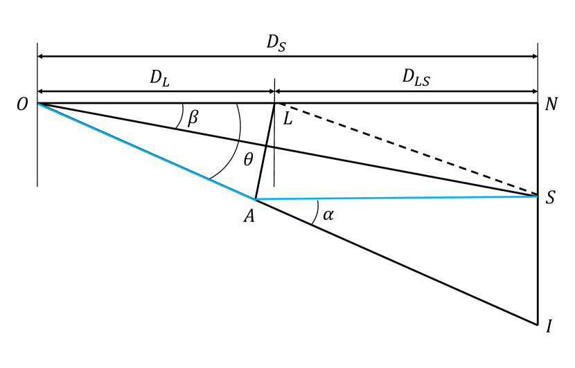
(a) Image 1

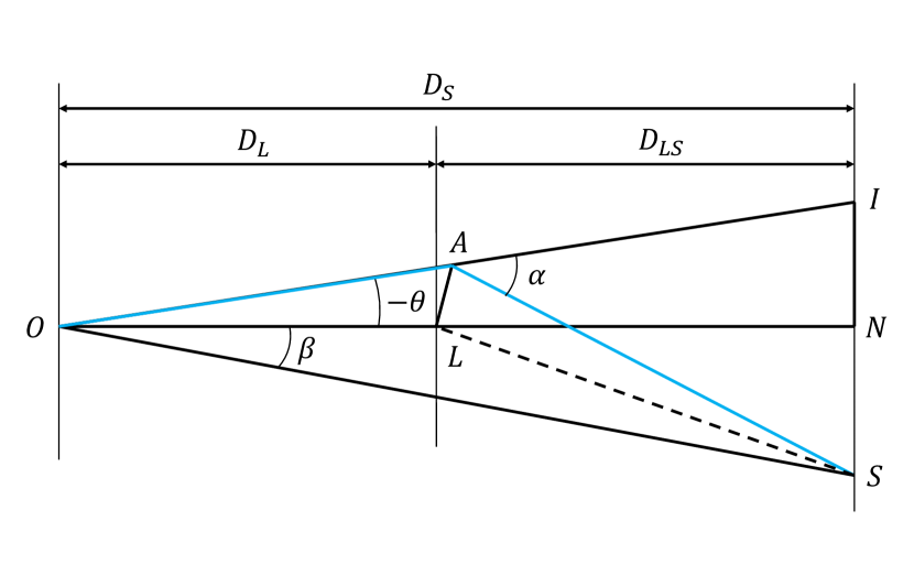
(b) Image 2

Figure 1: Geometrical configuration of gravitational lensing system (left: for image 1, right: for image 2). The points O, L, and S represent the observer, lens object, and wave source. The straight line ON is the optical axis. The planes passing through the lens and source, and being vertical to the optical axis are the lens plane and source plane. The distances from the observer to the lens and source plane are denoted by $D_{L}$ and $D_{S}$, and then $D_{LS}=D_{S}-D_{L}$. $\alpha$ is the deflection angle. $\beta$ and $\theta$ are the angular coordinates of the source and image.

Table 1: We list all of the example values of the lensing parameters involved in our discussion. We have fixed $D_{L}=780M$ and $D_{LS}=750M$, and the system is completely determined by source position. The first two columns are the (normalized) source coordinates. The rest of the columns are the normalized image coordinates, deflection angle, impact parameter, magnification, and axis ratio, for the two images produced by the Schwarzschild lensing.

$\beta_{0}\equiv\beta/\theta_{E}$	$\beta\,({\mathrm{rad}})$	$\theta_{0}\equiv\theta/\theta_{E}$	$\alpha\,({\mathrm{rad}})$	$b$	$u_{m}$	$\lambda_{c}(M)$	$\mu$	$\mathcal{R}$
$0.2$	$0.0100276$	$+1.1049880$	$0.0961826$	$44.57491$	$0.0229677$	/	$+3.0300350$	$+0.0932811$
		$-0.9049876$	$0.1174096$	$37.06395$	$0.0277617$	$1295.4090$	$-2.0459700$	$-0.0910933$
$0.4$	$0.0200552$	$+1.2198040$	$0.0870816$	$48.91776$	$0.0208831$	/	$+1.8169000$	$+0.1857575$
		$-0.8198039$	$0.1294972$	$33.88811$	$0.0304500$	$1152.5960$	$-0.8320377$	$-0.1772210$
$0.6$	$0.0300828$	$+1.3440310$	$0.0789617$	$53.63810$	$0.0190082$	/	$+1.4357270$	$+0.2746534$
		$-0.7440307$	$0.1424925$	$31.07548$	$0.0333071$	$1058.9230$	$-0.4496574$	$-0.2561892$
$0.8$	$0.0401105$	$+1.4770330$	$0.0717680$	$58.71282$	$0.0173352$	/	$+1.2607480$	$+0.3577646$
		$-0.6770330$	$0.1563105$	$28.59841$	$0.0363085$	$994.5211$	$-0.2732032$	$-0.3265907$

In Fig. 2, we display the evolution of the first four terms in the Dyson-like series in Eq. (20). The first two terms $\mathcal{I}_{0}=\lambda$, shown as a straight line with slope $1$, and $\mathcal{I}_{1}$ are the dominant terms of the geodesic deviation vector. There is an obvious turning point at $\lambda/M\sim 750$, because the external gravitational field deflects the photon/graviton path by slightly different angles. The subsequent two terms, $\mathcal{I}_{2}$ and $\mathcal{I}_{3}$, are almost always zero because they represent high-order weak-deflection correction. This also indicates that the Dyson-like series converges under the weak-deflection limit.

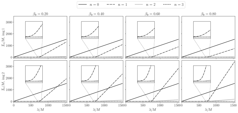
Figure 2: The evolution of each term in Dyson-like series (19) along the geodesic. These curves are plotted based on the analytical solution shown in Eqs. (80, 82, 83, 84, 85).

Fig. 3 shows the evolution of the transversal components of the geodesic deviation vector along the null geodesics. Before entering the external gravitational field, the evolutions of $\tilde{\xi}_{+}$ and $\tilde{\xi}_{-}$ are almost equal. However, the slopes of $\tilde{\xi}_{+}$ and $\tilde{\xi}_{-}$ are obviously different after leaving the gravitational field. From the expressions of tetrad leg $m^{\mu}$, we conclude that $\tilde{\xi}_{+}$ lies on the equatorial plane of the Schwarzschild black hole, and $\tilde{\xi}_{-}$ is vertical to that. Due to the tidal force, $\tilde{\xi}_{+}$ always increases, and the increasing rate gets larger after leaving the lens object than before entering. Distinguishingly, the growth of $\tilde{\xi}_{-}$ is always suppressed. For relatively large $b$, the tidal force is strong enough to make $\tilde{\xi}_{-}$ decrease rapidly enough, as shown in the second line of Fig. 3, $\tilde{\xi}_{-}$ arrives at zero at the moment, where the cross-sectional area and axis ratio tend to $0$. This point is usually called a caustic point, denoted by $\lambda_{c}$ and determined by $\tilde{\xi}_{-}(\lambda_{c})=0$. In this case, the detected lensing image is inverted (negative parity). Conversely, when the impact parameter is relatively small, there is no caustic point, and $\tilde{\xi}_{-}$ remains positive on the entire path, ultimately resulting in an upright (positive parity) image. Besides the approximate analytical solution, we implement the numerical solution to Eq. (13), with initial values being $\xi_{\pm}(\lambda=0)=0$ and $\bm{\mathcal{D}}\xi_{\pm}(\lambda=0)=1$. These results are also plotted in Fig. 3, verifying that the Dyson-like series solution is valid under the weak deflection and thin lens limits.

As shown in Eq. (24) and around it, we can define the cross-sectional area ($\mathcal{A}$) and axis ratio ($\mathcal{R}$) from the deviation vector. Fig. 4 depicts their evolution along the path. The area and axis ratio are always positive for image 1 (the left panels), but meet zero at the caustic point for image 2 (the right panels). The relative changing rates of $\mathcal{A}$ and $\mathcal{R}$ are described by optical scalars, $\rho$ and $\sigma$, respectively, which are shown in Fig. 5. When closing to the wave source (point like as we have assumed), all of the geodesics in congruence focus on a point, and subsequently, $\rho$ is infinity. At the starting point, $\tilde{\xi}_{+}$ and $\tilde{\xi}_{-}$ are set to the same initial conditions, such that $\sigma$ is keeping to zero before approaching the lens object. More importantly, in image 1, these two optical scalars are continuous, but there is a discontinuity in image 2, caused by the caustic point.

The weak deflection and thin-lens approximation bring errors in the analytical solutions. For example, one can find slight deviations between the slopes of the numerical and analytical solutions to $\tilde{\xi}_{\pm}$ (see Fig. 3). Such error is amplified when calculating $\sigma$, especially when approaching the observer (see the left-bottom panel in Fig. 5). It is noted that the example parameters in Table 1 significantly deviate from the realistic situation. A typical lens object has mass $M\sim 10^{8}M_{\odot}$ and redshift $z\sim 1$. The angular separation of the image and lens is about $\theta\sim 1^{\prime\prime}$. We can estimate the distance and impact parameter for such a system as $D_{L}\approx 4.3\times 10^{3}\,\mathrm{Mpc}\approx 9.0\times 10^{14}M$ and $b\sim 4.8\times 10^{-6}D_{L}$. This estimation indicates that the impact distance is much greater than the Schwarzschild radius, and $D_{L}$ is much greater than the impact distance, ensuring the validity of the weak deflection and thin lens approximations.

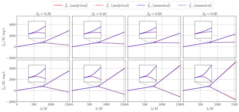
Figure 3: The evolution of the transversal components of the geodesic deviation vector, $\tilde{\xi}_{\pm}$ from different source positions and images. The red curves show the evaluated results based on the analytical expressions from the Dyson-like series (20). The blue curves are obtained by numerically solving the GDE (13), together with the radial geodesic equation in Eq. (26).

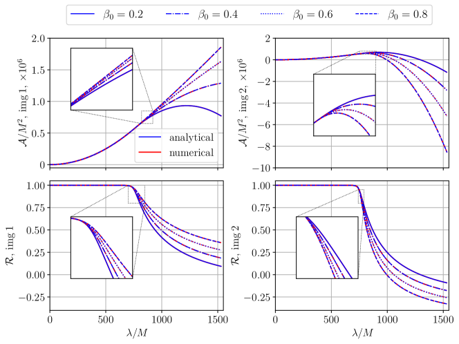
Figure 4: The evolution of the area and axis ratio of the geodesic congruence. Same with Fig. 3, the blue and red curves are obtained from the analytical solutions and corresponding numerical solutions to Eq. (13).

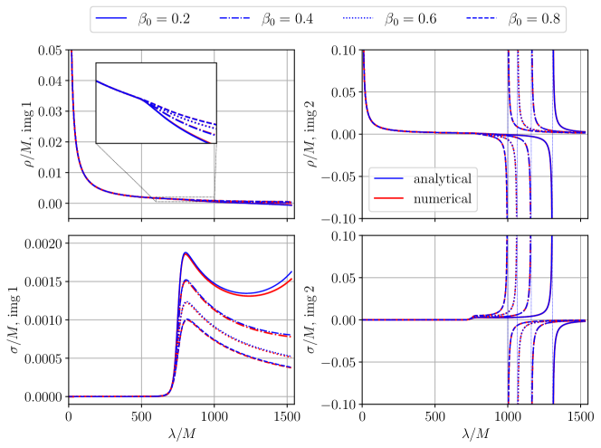
Figure 5: The evolution of the spin coefficients $\rho$ and $\sigma$. Same with Fig. 3, the blue and red curves are obtained from the analytical solutions and corresponding numerical solutions to Eq. (13). The vertical dotted lines in the right panels represent the caustic points. The corresponding values are listed in Table 1.

IV.3 The magnification and axis ratio of the lensing images

In the last subsection, we investigate the behaviors of the geodesic deviation vector, cross-sectional area/axis ratio, and optical scalars along the lensing path. In this subsection, we study the observational imprints by such evolution. The magnification of the lensing image is defined as the ratio between the lensed and unlensed energy flux at the observer. In geometric optics, the energy flux of light and GWs is covariantly conserved within the congruence, and then proportional to $1/\mathcal{A}$. Therefore, the magnification is rewritten as

$$\mu=\frac{\widehat{\mathcal{A}}(\lambda_{o})}{\mathcal{A}(\lambda_{o})}.$$ (34)

$\widehat{\mathcal{A}}$ means the cross-sectional area of a congruence freely propagating along the unlensed path (OS, see Fig. 1). By setting the initial conditions as $\widehat{\mathcal{A}}(\lambda=0)=0$ and $\bm{\mathcal{D}}\widehat{\mathcal{A}}(\lambda=0)=1$, its solution is given by

$$\widehat{\mathcal{A}}(\lambda)=\frac{1}{\mathrm{OS}^{2}},\quad\text{with}\quad\text{OS}=D_{S}\sqrt{1+\tan^{2}\beta}=\frac{r_{o}}{\sqrt{1+\tan^{2}\beta}}\left[1+\sqrt{1-(1+\tan^{2}\beta)\left(1-\frac{r_{s}^{2}}{r_{o}^{2}}\right)}\right].$$ (35)

We recall that $r_{s}$ and $r_{o}$ are the radial Schwarzschild coordinates of the source and observer, relating $D_{L}$ and $D_{S}$ by

$$r_{o}=D_{L},\quad\text{and},\quad r_{s}=D_{S}^{2}(1+\tan^{2}\beta)-2D_{L}D_{S}+D_{L}^{2}$$ (36)

The area of the lensed congruence is calculated from the Dyson-like series (20). At the observer position, we get the expressions of the first four terms in this series,

$$\mathcal{I}_{0}(\lambda_{o})=\lambda_{o}\approx\frac{M}{u_{m}}\left(\frac{1}{x_{s}}+\frac{1}{x_{o}}\right)\left[1-\frac{1}{2}x_{s}x_{o}\left(1-\frac{4u_{m}}{x_{s}+x_{o}}\right)\right],$$ (37)

$$\mathcal{I}_{1}(\lambda_{o})\approx\frac{2M}{x_{s}x_{o}}\left\{2+\left(\frac{45\pi}{16}-4\right)u_{m}+\left[\left(\frac{192}{5}-\frac{135\pi}{16}\right)u_{m}^{2}+2u_{m}(x_{s}+x_{o})-(x_{s}^{2}-x_{s}x_{o}-x_{o}^{2})\right]\right\},$$ (38)

$$\mathcal{I}_{2}(\lambda_{o})\approx\frac{M}{x_{s}x_{o}}\left\{\frac{15\pi}{8}u_{m}+u_{m}\left[\left(48-\frac{45\pi}{8}\right)u_{m}-4(x_{s}+x_{o})\right]\right\},$$ (39)

and

$$\mathcal{I}_{3}(\lambda_{o})\approx\frac{M}{x_{s}x_{o}}\cdot\frac{16}{5}u_{m}^{2}.$$ (40)

Under the weak deflection and thin-lens assumptions, $u_{m}\ll 1$, and $x_{s,o}\equiv r_{m}/r_{s,o}\ll 1$ with the same order of $u_{m}$, we have expanded the expressions in terms of small parameters $u_{m}$, $x_{s}$, and $x_{o}$, up to the zeroth order, in Eqs. (37 - 40). Inserting Eqs. (37 - 40) into Eq. (19), and then into the definition Eq. (23), the area $\mathcal{A}(\lambda_{o})$ is obtained. Then, combining this result with the unlensed area in Eq. (35), the magnification is given from its definition Eq. (34).

However, the parameters used here are different with those in the standard textbook Schneider et al. (1992), and we transform them into the commonly used lensing parameter as follows. (1) Transform $u_{m}$ into $b$ by Eq. (63), and then, from the geometry shown in Fig. 1, $b=\pm D_{L}\sin\theta/M$ for image 1 and 2, respectively. (2) Transform $x_{s}$ and $x_{o}$ into $\beta$, $D_{L}$, and $D_{LS}$ by their definition and Eq. (36). (3) Substitute the relation between $\beta$ and $\theta$ from lens equation (72, 72). (4) In the weak deflection and thin lens limit, we expand the image position as

$$\theta=\theta_{E}\left[\theta_{0}+\theta_{1}\epsilon+\theta_{2}\epsilon^{2}+\mathcal{O}(\epsilon^{3})\right],$$ (41)

where the bookkeeper is of order,

$$\epsilon\sim\frac{\theta_{E}}{4\mathcal{D}},\quad\text{with}\quad\mathcal{D}\equiv\frac{D_{LS}}{D_{S}}.$$ (42)

After the above operations, we obtain the final result of the magnification, which is expanded in powers of $\epsilon$ as

$$\mu =\frac{\theta_{0}^{4}}{\theta_{0}^{4}-1}\mp\frac{15\pi\theta_{0}^{3}}{16(1+\theta_{0}^{2})^{3}}\cdot\epsilon+\frac{\theta_{0}^{2}}{384(1-\theta_{0}^{2})^{2}(1+\theta_{0}^{2})^{5}}\Bigg{\{}-1024(3-2\mathcal{D}^{2})$$ (43)

$$\quad+1024(9+12\mathcal{D}-14\mathcal{D}^{2})\theta_{0}^{2}+[4096(3-\mathcal{D}^{2})-2025\pi^{2}]\theta_{0}^{4}-\left[2048(6+15\mathcal{D}-17\mathcal{D}^{2})-2025\pi^{2}\right]\theta_{0}^{6}$$

$$\quad-1024(9+6\mathcal{D}-8\mathcal{D}^{2})\theta_{0}^{8}+1024\mathcal{D}(3+18\mathcal{D}-20\mathcal{D}^{2})\theta_{0}^{10}+6144\mathcal{D}(1-\mathcal{D})\theta_{0}^{12}\Bigg{\}}\epsilon^{2}+\mathcal{O}(\epsilon^{3}),$$

The leading-order result can be found in several standard textbooks, e.g., Schneider et al. (1992). For the case where $\theta=\theta_{E}$, and $\theta_{0}=1$, the magnification tends to infinity. The positions with infinite magnification is defined as the critical curve. When the image is located at the outside/inside of the critical curve, the magnification is positive/negative, as shown in Table 1, representing whether the image is upright (positive parity) or inverted (negative parity). In the second-order terms, the $\pm$ corresponds to image 1 and image 2. The higher-order corrections are derived by Ref. Keeton and Petters (2005), through the Jacobian matrix. In Appendix E, we compare our result (43) with the previous work Keeton and Petters (2005).

Another direct observational quantity is the axis ratio of the images, describing the shape distortion of the background wave source. Similar to the deduction of magnification, the axis ratio $\mathcal{R}(\lambda_{o})$ is given by,

$$\mathcal{R} =\frac{\theta_{0}^{2}-1}{\theta_{0}^{2}+1}\mp\frac{15\pi(\theta_{0}^{2}-1)(1+3\theta_{0}^{2})}{16\theta_{0}(1+\theta_{0}^{2})^{3}}\cdot\epsilon+\frac{(\theta_{0}^{2}-1)}{768\theta_{0}^{2}(1+\theta_{0}^{2})^{5}}\Bigg{\{}-9(2048-225\pi^{2})$$ (44)

$$\quad-[4096(18+3\mathcal{D}-4\mathcal{D}^{2})-8100\pi^{2}]\theta_{0}^{2}-3[4096(6+\mathcal{D}-\mathcal{D}^{2})-3375\pi^{2}]\theta_{0}^{4}$$

$$\quad-8193\mathcal{D}^{2}\theta_{0}^{6}+6144(3-2\mathcal{D}+2\mathcal{D}^{2})\theta_{0}^{8}-4096\mathcal{D}(3-4\mathcal{D})\theta_{0}^{10}\Bigg{\}}\epsilon^{2}+\mathcal{O}(\epsilon^{3}).$$

When the lensing image is located at the critical curve, with $\theta_{0}=1$, the axis ratio is zero. This means the extended source is distorted to be a line segment, with zero area and infinite amplitude. Similar to the magnification, the axis ratio is positive/negative for the images located outside/inside of the critical curve, representing whether the image is upright (positive parity) or inverted (negative parity). The numerical results of $\mathcal{R}$ are listed in Table 1.

The magnification and axis ratio are related to the convergence ($\kappa$) and shear ($\gamma_{1}$ and $\gamma_{2}$) by

$$\mu=\frac{1}{(1-\kappa)^{2}-\gamma^{2}},\quad\text{and}\quad\mathcal{R}=\frac{1-\kappa-\gamma}{1-\kappa+\gamma},$$ (45)

with $\gamma=\sqrt{\gamma_{1}^{2}+\gamma_{2}^{2}}$. The convergence depends on the lens mass density within the geodesic congruence. The shear $\gamma_{1}$ characterizes the stretching of the lensing images and $\gamma_{2}$ characterizes its orientation. For the Schwarzschild lens, that is vacuum and axisymmetric, $\kappa=0$, $\gamma_{2}=0$, and $\gamma=\gamma_{1}$. Through the Jacobian matrix Schneider et al. (1992), the shear of the point-mass lens is calculated as $\gamma=1/\theta_{0}^{2}$ at the leading order of weak deflection approximation, resulting in $\mu=\theta_{0}^{4}/(\theta_{0}^{4}-1)$ and $\mathcal{R}=(\theta_{0}^{2}-1)/(\theta_{0}^{2}+1)$, as shown in the leading terms of Eqs. (43) and (44).

V Conclusion

In this work, we revisit the Schwarzschild lensing of light or GWs from geodesic deviation. The detected lensed signal consists of a congruence of light/gravitational rays, and their collective behavior is described by the GDE. To solve it, we project the GDE onto the NP tetrad constructed along the null geodesics and get a pair of decoupled equations for $\xi_{+}$ and $\xi_{-}$ (13) for real Weyls scalar $\Psi_{0}$. Similar to the Dyson series, we present the solution to the transversal components of the deviation vector in Eqs. (19) and (20). In addition, the relationship between the deviation vector and the optical scalars, $\rho$ and $\sigma$, is presented in Eq. (11). The physical meaning of these two scalars is the relative changing rate of the congruence cross section and the axis ratio [see Eq. (22)].

Subsequently, we consider the lensing process in the weak deflection limit, where the impact parameter is sufficiently large. The general signature is shown in Fig. 1, two images are formed by Schwarzschild lensing. In this assumption, the Dyson-like series is calculated from Eq. (31, 32) analytically. We depict such results in Fig. 2, and compare them with the numerical solution for a group of parameters listed in Table 1. And we find that $\mathcal{I}_{0}$ and $\mathcal{I}_{1}$ are dominant and $\mathcal{I}_{2},\,\mathcal{I}_{3}$ are close to zero, implying the series (19) is convergent in weak deflection limit. Fig. 3 shows the evolution of the deviation vector. $\tilde{\xi}_{+}$ increases more rapidly after lensing and keeps positive. And $\tilde{\xi}_{-}$ increases more slowly or even decreases after lensing, meeting the caustic point, and finally forms an inverted image at the observer. Correspondingly, Figs. 4 and 5 show the cross-sectional area, axis ratio, and optical scalars, defined in Eqs. (23, 24).

In subsection IV.3, we reproduce the magnification from the geodesic deviation [see Eq. (43)], consistent with that from the Jacobian matrix in Ref. Keeton and Petters (2005). Meanwhile, we find some missing corrections in the previous calculation, e.g., the deflection point deviates from the lens plane and the lens equations are slightly different for the two images. Additionally, we present the result of the axis ratio, equivalently, the shear, of lensing images up to the second weak deflection approximation [see Eq. (44)].

This work is potentially worthwhile for future studies. As discussed in Ref. Dolan (2018b); Shipley (2019), the calculation of spin coefficients is indispensable when investigating the lensing effects beyond geometric optics, in which richer information on light and GW polarization is presented Harte (2019a, b); Cusin and Lagos (2020); Dalang et al. (2022); Li et al. (2022); Kubota et al. (2024). In this work, we calculate $\rho$ and $\sigma$ following the procedure in Ref. Dolan (2018a) in the simplest case, the Schwarzschild lensing. Furthermore, the astrophysical lens objects are more complex than a Schwarzschild black hole Keeton (2002). Extending the computation to a more general lens model is helpful to the lensing observation and gravitational testing in the future.

Appendix A Null tetrad in Kerr spacetime

In this section, we review the main procedure to construct the null tetrad in Kerr spacetime, shown in Ref. Dahal (2023). Let us denote the Boyer-Lindquist coordinate as $\{t,r,\theta,\varphi\}$, the background metric as $g_{\mu\nu}$, the black hole mass as $M$, and spin as $a$ in this section. Before construction, it is necessary to summarize several important tensors. The first one is the principal tensor,

$$\gamma_{\mu\nu}=\left(\begin{array}[]{cccc}0&r&a^{2}\sin\theta\cos\theta&0\\ -r&0&0&ar\sin^{2}\theta\\ -a^{2}\sin\theta\cos\theta&0&0&a(r^{2}+a^{2})\sin\theta\cos\theta\\ 0&-ar\sin^{2}\theta&-a(r^{2}+a^{2})\sin\theta\cos\theta&0\\ \end{array}\right),$$ (46)

satisfying $\nabla_{\alpha}\gamma_{\mu\nu}=g_{\alpha\mu}\xi_{\nu}-g_{\alpha\nu}\xi_{\mu}$, where $\xi^{\mu}=(1,0,0,0)$ is the Killing vector, indicating the energy conservation of the particle moving along the geodesics. Its Hoge dual defines the Killing-Yano tensor by

$$f_{\mu\nu}\equiv-\hat{\gamma}_{\mu\nu}=-\frac{1}{2}\sqrt{-g}\epsilon_{\alpha\beta\mu\nu}\gamma^{\alpha\beta}=\left(\begin{array}[]{cccc}0&-a\cos\theta&ar\sin\theta&0\\ a\cos\theta&0&0&-a^{2}\sin^{2}\theta\cos\theta\\ -ar\sin\theta&0&0&r(r^{2}+a^{2})\sin\theta\\ 0&a^{2}\sin^{2}\theta\cos\theta&-r(r^{2}+a^{2})\sin\theta&0\\ \end{array}\right),$$ (47)

satisfying $\nabla_{(\alpha}f_{\mu\nu)}=0$. $\epsilon_{\alpha\beta\mu\nu}$ is Levi-Civita symbol.

Firstly, we need to construct a set of basis vectors, denoted by $\{\bm{\lambda}_{(1)},\bm{\lambda}_{(2)},\bm{\lambda}_{(3)},\bm{\lambda}_{(4)}\}$, as follows,

$$\lambda_{(1)}^{\alpha}=k^{\alpha},$$ (48)

$$\lambda_{(3)}^{\alpha}=\gamma^{\alpha\beta}\lambda^{(1)}_{\beta}-A(r,\theta)\lambda_{(1)}^{\alpha},$$ (49)

$$\lambda_{(2)}^{\alpha}=\gamma^{\alpha\beta}\lambda^{(3)}_{\beta}-B(r,\theta)\lambda_{(1)}^{\alpha},$$ (50)

$$\lambda_{(4)}^{\alpha}=f^{\alpha}_{\ \ \beta}\lambda_{(1)}^{\beta},$$ (51)

The wavevector in Kerr spacetime is presented by

$$\lambda_{(1)}^{\alpha}=k^{\alpha}=\left\{\frac{(r^{2}+a^{2})^{2}-a^{2}\Delta\sin^{2}\theta-2M\xi ar}{\Delta\Sigma},\frac{\mathcal{R}}{\Sigma},\frac{\Theta}{\Sigma},\frac{2Mar+(\Sigma-2Mr)\xi\csc^{2}\theta}{\Delta\Sigma}\right\},$$ (52)

with $\Delta\equiv r^{2}(1-2M/r+a^{2}/r^{2})$ and $\Sigma\equiv r^{2}+a^{2}\cos^{2}\theta$. $A(r,\theta)$ and $B(r,\theta)$ are two underdetermined functions. $\xi,\eta$ being the conserved angular momentum, and Carter constant. The first leg is parallel-transported. Letting the third leg be parallel-transported, we get the constraint on the unknown functions,

$$\frac{dA}{d\lambda}=\xi^{\beta}k_{\beta},\quad\text{and}\quad\frac{dB}{d\lambda}=h^{\gamma\beta}\xi_{\gamma}k_{\beta}-\frac{1}{2}\frac{dA^{2}}{d\lambda}.$$ (53)

From the above equation, one can find that the function $B$ is determined by directly integrating on the right-hand side once $A$ is given. Based on the above discussion, we can list all of the expressions of the tetrad. The third one is

$$\lambda_{(3)}^{\alpha}= \left(\begin{array}[]{c}\{a^{2}\sin^{2}\theta/\Sigma-[(r^{2}+a^{2})^{2}-2Ma\xi r]/\Delta\Sigma\}A-r(r^{2}+a^{2})\mathcal{R}/\Delta\Sigma-(\Theta/\Sigma)a^{2}\sin\theta\cos\theta\\ -r(r^{2}+a^{2}-a\xi)/\Sigma-(\mathcal{R}/\Sigma)A\\ a\cot\theta(\xi-a\sin^{2}\theta)/\Sigma-(\Theta/\Sigma)A\\ -[2Mar+(\Sigma-2Mr)\xi\csc^{2}\theta]A/(\Delta\Sigma)+a[(\Theta/\Sigma)\cot\theta+(r/\Delta)(\mathcal{R}/\Sigma)],\end{array}\right)$$ (54)

Using the known Killing vector, the constraint on $A(r,\theta)$ becomes $dA/d\lambda=-1$. We shall suppose that the function $A$ is variable-separable, which gives the form $A(r,\theta)=\mathcal{F}(r)+\mathcal{G}(\theta)$. An obvious set of solutions is

$$\mathcal{F}(r)=-\int\frac{r^{2}}{\mathcal{R}}dr,\quad\mathcal{G}(\theta)=-\int\frac{a^{2}\cos^{2}\theta}{\Theta}d\theta.$$ (55)

Using the principal tensor (46) and Killing vector, the constraint on $B$ becomes

$$B(r,\theta)=\frac{1}{2}[r^{2}-a^{2}\cos^{2}\theta-A^{2}(r,\theta)].$$ (56)

And then the second leg is

$$\lambda_{(2)}^{t} =-(1/2)(r^{2}-a^{2}\cos^{2}\theta-A^{2})\{(r^{2}+a^{2})^{2}-a^{2}\Delta\sin^{2}\theta-2aM\xi r\}/(\Delta\Sigma)$$ (57)

$$\qquad+r(r^{2}+a^{2})(\mathcal{R}A+a^{2}r-a\xi r+r^{3})/(\Sigma\Delta)$$

$$\qquad\qquad+a^{2}\cos\theta[\Theta\sin\theta A+a\cos\theta(a\sin^{2}\theta-\xi)]/\Sigma,$$

$$\lambda_{(2)}^{r} =\{2rA[(r^{2}+a^{2})-a\xi]+\mathcal{R}(\Sigma+A^{2})\}/(2\Sigma),$$

$$\lambda_{(2)}^{\theta} =\left[-2a\cot\theta A(\xi-a\sin^{2}\theta)+\Theta A^{2}-\Sigma\Theta\right]/(2\Sigma),$$

$$\lambda_{(2)}^{\varphi} =(A^{2}+a^{2}\cos^{2}\theta-r^{2})[a^{2}\xi\cot^{2}\theta+2aMr+\xi r\csc^{2}\theta(r-2M)]/(2\Delta\Sigma)$$

$$\qquad+2ar(\mathcal{R}A+a^{2}r-a\xi r+r^{3})/(\Delta\Sigma)-a\cot\theta(a\cot\theta(\xi-a\sin^{2}\theta)-A\Theta)/\Sigma,$$

and the fourth leg is

$$\lambda_{(4)}^{\alpha}=\left(\begin{array}[]{c}a[\mathcal{R}(r^{2}+a^{2})\cos\theta-r\Theta\sin\theta\Delta]/(\Sigma\Delta)\\ a\cos\theta[(r^{2}+a^{2})-a\xi]/\Sigma\\ r\csc\theta(\xi-a\sin^{2}\theta)/\Sigma\\ \csc\theta(a^{2}\mathcal{R}\sin\theta\cos\theta-r\Delta\Theta)/(\Delta\Sigma)\end{array}\right).$$ (58)

After constructing $\{\bm{\lambda}_{(1)},\bm{\lambda}_{(2)},\bm{\lambda}_{(3)},\bm{\lambda}_{(4)}\}$, the NP tetrad is defined by

$$e_{(a)}^{\alpha}=\left\{\lambda_{(1)}^{\alpha},\frac{1}{\mathscr{C}^{2}}\lambda_{(2)}^{\alpha},\frac{1}{\mathscr{C}}\frac{1}{\sqrt{2}}\left[\lambda_{(3)}^{\alpha}+i\lambda_{(4)}^{\alpha}\right],\frac{1}{\mathscr{C}}\frac{1}{\sqrt{2}}\left[\lambda_{(3)}^{\alpha}-i\lambda_{(4)}^{\alpha}\right]\right\},$$ (59)

which satisfies the orthogonality and parallel-transported condition. The normalization constant is

$$\mathscr{C}\equiv\sqrt{(a-\xi)^{2}+\eta}.$$ (60)

Appendix B Schwarzschild lensing

One defines $u\equiv M/r$, and then the photon/graviton trajectory is dominated by Chandrasekhar (1983)

$$\left(\frac{du}{d\varphi}\right)^{2}=\frac{1}{b^{2}}-u^{2}(1-2u)\equiv f(u),$$ (61)

The impact parameter is $b=|L|/M$. When $b>3\sqrt{3}$, the function $f(u)$ possesses two different zero points, denoted by $0<u_{2}<u_{3}$, the allowed orbits should be located at interval $[0,u_{2}]$ and $[u_{3},+\infty]$, where $f(u)>0$. These first kinds of orbits are open, in which the massless particle moves between an infinite region and a pericenter, corresponding to the gravitational lensing situation. The radial range of allowed motion is $r_{0}<r<\max\{r_{o},r_{s}\}$, or equivalently, $\min\{u_{o},u_{s}\}<u<u_{m}\equiv M/r_{m}$. $r_{o}$ and $r_{s}$ denote the radial coordinates of the wave source and observer. correspondingly, $u_{o}\equiv M/r_{o}$ and $u_{s}\equiv M/r_{s}$.

In this work, we only focus on the weak deflection limit and thin lens approximation, in which the impact distance ($Mb$) is much larger than the gravitational radius of the lens black hole, and the distances from emitter/observer to lens object are very larger than the impact distance. Using a bookkeeper, $\epsilon$, the order of magnitude impact parameter, source/observer distance are

$$u_{m}\sim\frac{1}{b}\sim\epsilon,\quad\frac{r_{m}}{r_{s}},\frac{r_{m}}{r_{o}}\sim\epsilon.$$ (62)

The following calculations are based on the Taylor expansion by the bookkeeper $\epsilon$. Additionally, the explicit relationship between $u_{m}$ and $b$ is given by $f(u_{m})=0$,

$$b=\frac{1}{u_{m}}\frac{1}{\sqrt{1-2u_{m}}}=\frac{1}{u_{m}}\left[1+u_{m}+\frac{3}{2}u_{m}^{2}+\frac{5}{2}u_{m}^{3}+\mathcal{O}(u_{m}^{4})\right].$$ (63)

Following the standard steps, the trajectory equation $u=u(\varphi)$ is

$$u=u_{m}\cos\varphi+u_{m}^{2}\left(1-\cos\varphi+\sin^{2}\varphi\right)+u_{m}^{3}\left[\left(2-\frac{3}{4}\sin^{2}\varphi\right)\cos\varphi-2(1+\sin^{2}\varphi)+\frac{15}{4}\varphi\sin\varphi\right]+\mathcal{O}(u_{m}^{3}),$$ (64)

Up to order $\mathcal{O}(u_{m}^{3})$. The deflection angle, $\alpha$, is obtained from the asymptotic behavior of solution (64), given by

$$\alpha=4u_{m}+\left(-4+\frac{15}{4}\pi\right)u_{m}^{2}+\left(\frac{122}{3}-\frac{15\pi}{2}\right)u_{m}^{3}.$$ (65)

After giving the deflection angle (65), we re-drive the lens equation in this appendix. We first investigate image 1 shown in Fig. 1(a), in which the source and image lie on the same side of the optical axis. In $\triangle$ASI, applying the sine theorem gives,

$$\frac{\text{SI}}{\sin\alpha}=\frac{\text{AI}}{\sin\angle\text{ASI}}\quad\Rightarrow\quad\frac{\text{NI}-\text{SN}}{\sin\alpha}=\frac{\text{OI}-\text{OA}}{\sin[\pi/2-(\alpha-\theta)]}=\frac{\text{OI}-\text{OA}}{\cos(\alpha-\theta)},$$ (66)

where we use $\angle\text{ASI}=\pi-\alpha-\angle\text{AIS}=\pi-\alpha-(\pi/2-\theta)=\pi/2-(\alpha-\theta)$ and then

$$\left(\frac{\text{NI}}{\text{OI}}-\frac{\text{SN}}{\text{OI}}\right)\cos(\alpha-\theta)=\left(1-\frac{\text{OA}}{\text{OI}}\right)\sin\alpha,$$ (67)

or, equivalently

$$\left(\frac{D_{S}\tan\theta-D_{S}\tan\beta}{D_{S}\sec\theta}\right)\cos(\alpha-\theta)=\left(1-\frac{\text{OA}}{D_{S}\sec\theta}\right)\sin\alpha.$$ (68)

Then the length of line OA can be expressed from the $\triangle$OAL by sine theorem,

$$\frac{\text{OL}}{\sin\angle\text{OAL}}=\frac{\text{OA}}{\sin\angle\text{OLA}}.$$ (69)

Here, the line AL divides $\angle$OAS equally, such that the above equation becomes

$$\frac{D_{L}}{\sin(\pi-\alpha)/2}=\frac{\text{OA}}{\sin[\pi-\theta-(\pi-\alpha)/2]}.$$ (70)

Using the expression of OA in terms of $D_{L}$, $\theta$, and $\alpha$,

$$\text{OA}=D_{L}\frac{\cos(\alpha/2-\theta)}{\cos(\alpha/2)}.$$ (71)

We finally arrived at

$$\left(\tan\theta-\tan\beta\right)\cos\theta\cos(\alpha-\theta)=\sin\alpha-\frac{2D_{L}}{D_{S}}\cos\left(\frac{\alpha}{2}-\theta\right)\cos\theta\sin\frac{\alpha}{2}.$$ (72)

By replacing $\theta$ by $-\theta$, and $\beta$ by $-\beta$ (equivalently, replace $\mathrm{NI}-\mathrm{SN}$ by $\mathrm{NI}+\mathrm{SN}$) in Eq. (72), we get the lens equation for image 2,

$$-\left(\tan\theta-\tan\beta\right)\cos\theta\cos(\alpha+\theta)=\sin\alpha-\frac{2D_{L}}{D_{S}}\cos\left(\frac{\alpha}{2}+\theta\right)\cos\theta\sin\frac{\alpha}{2},$$ (73)

in which the source and image lie on the different sides of the optical axis.

To solve the lens equation (72, 73), we rescale the source position and image position as

$$\beta=\beta_{0}\theta_{E},\quad\theta=\theta_{E}\left[\theta_{0}+\theta_{1}\epsilon+\theta_{2}\epsilon^{2}+\mathcal{O}(\epsilon^{3})\right],$$ (74)

where the bookkeeper $\epsilon$ is defined in Eq. (42). Then the lens equation at leading order is simplified as

$$\beta_{0}=\theta_{0}-\frac{1}{\theta_{0}},$$ (75)

at the leading order, whose solution is

$$\theta_{0}=\frac{1}{2}\left[\beta_{0}\pm\sqrt{\beta_{0}^{2}+4}\right].$$ (76)

In the second and third orders, the solutions to $\theta_{1}$ and $\theta_{2}$ are

$$\theta_{1}=\pm\frac{15\pi}{16(1+\theta_{0}^{2})},$$ (77)

and

$$\theta_{2} =\frac{1}{3\theta_{0}(1+\theta_{0}^{2})^{3}}\Bigg{\{}48-\frac{675}{256}\pi^{2}-16\mathcal{D}^{2}+\left[8(9-3\mathcal{D}+2\mathcal{D}^{2})-\frac{675}{128}\pi^{2}\right]\theta_{0}^{2}$$ (78)

$$\qquad\qquad\qquad+40\mathcal{D}^{2}\theta_{0}^{4}-8(3-9\mathcal{D}+4\mathcal{D}^{2})\theta_{0}^{6}+8\mathcal{D}(6-5\mathcal{D})\theta_{0}^{8}\Bigg{\}}.$$

The plus-minus symbol corresponds to the image 1 and 2, respectively. The leading-order result (76) is consistent with Ref. Keeton and Petters (2005), but there is an extra plus-minus symbol in first-order correction (77). And the second-order result (78) is different, because the deflection point deviates from the lens plane.

Appendix C Solution to the radial motion

In weak deflection limit, the radial potential reduces to

$$U_{r}=\pm\sqrt{1-x^{2}}\left\{1-u_{m}\left(\frac{x^{2}}{1+x}\right)-u_{m}^{2}\left[\frac{x^{2}(2+x)^{2}}{2(1+x)^{2}}\right]\right\}+\mathcal{O}(u_{m}^{3}).$$ (79)

where $x\equiv u/u_{m}$, $u=M/r\leqslant u_{m}$, $u_{m}=M/r_{m}\ll 1$, with $r_{m}$ is the radius of pericenter. When the particle moves toward the pericenter, the above equation is integrated by

$$M^{-1}\lambda_{\rm I}=M^{-1}\int_{r_{s}}^{r}U_{r}^{-1}dr \approx-\frac{1}{u_{m}}\left(\frac{\nu}{x}-\frac{\nu_{s}}{x_{s}}\right)-\left(\frac{\nu}{1+x}-\frac{\nu_{s}}{1+x_{s}}\right)$$ (80)

$$\qquad+\frac{u_{m}}{2}\left[\frac{x\nu}{(1+x)^{2}}-\frac{x_{s}\nu_{s}}{(1+x_{s})^{2}}+3\arcsin x-3\arcsin x_{s}\right],$$

with initial condition $\lambda_{s}=0$. For simplicity, we define $\nu=\sqrt{1-x^{2}}$, and $\nu_{s}=\sqrt{1-x_{s}^{2}}$. When arriving the pericenter, $r=r_{m}$, where $x=1$, the affine parameter is

$$\lambda_{m}=\frac{1}{u_{m}}\frac{M}{x_{s}}\left[1+x_{s}\left(u_{m}-\frac{x_{s}}{2}\right)\right],$$ (81)

And then, when moving backward, the integration should be

$$M^{-1}\lambda_{\rm II} =M^{-1}\left\{\lambda_{m}+\int_{r_{m}}^{r}U_{r}^{-1}dr\right\}$$ (82)

$$\approx\frac{1}{u_{m}}\left(\frac{\nu}{x}+\frac{\nu_{s}}{x_{s}}\right)+\left(\frac{\nu}{1+x}+\frac{\nu_{s}}{1+x_{s}}\right)$$

$$\qquad-\frac{u_{m}}{2}\left[\frac{x\nu}{(1+x)^{2}}+\frac{x_{s}\nu_{s}}{(1+x_{s})^{2}}+3\arcsin x+3\arcsin x_{s}-3\pi\right].$$

And the affine parameter at the observer position has been shown in Eq. (37).

Appendix D The analytical expressions of Eqs. (31) and (32)

In this appendix, we present the analytical solution of Eqs. (31) and (32). The first three orders of the Dyson-like series are

$$M^{-1}\mathcal{I}_{1} =\pm\left(1+\frac{x_{s}}{x}-\frac{2}{xx_{s}}\right)\nu\pm\frac{u_{m}}{8xx_{s}(1+x)}\Big{\{}\Big{[}16(2+x)-(61+61x-15x^{2}-7x^{3})x_{s}$$ (83)

$$\quad+8xx_{s}^{2}+7(1+x)x_{s}^{2}\Big{]}\nu+15(3\nu\nu_{s}\pm xx_{s})\arccos x\Big{\}}\pm\frac{u_{m}^{2}}{40xx_{s}(1+x)^{2}}\Big{[}-8(192+364x+167x^{2})$$

$$\quad+(835+1709x+1143x^{2}+326x^{3}+119x^{4}+42x^{5})x_{s}+(543+1086x+523x^{2})x_{s}^{2}$$

$$\quad+35x(1+x)x_{s}^{3}+42(1+x)^{2}x_{s}^{4}\Big{]}\nu\mp\frac{3u_{m}^{2}}{8xx_{s}(1+x)(1+x_{s})}\Big{\{}\pm 15\left[3+2x+(2+x)x_{s}\right]\nu\nu_{s}$$

$$\quad+(1+x)\left[-8x-(8+13x-4x^{2})x_{s}-(8+x-4x^{2})x_{s}^{2}+4xx_{s}^{3}\right]\Big{\}}\arccos x\mp(x\leftrightarrow x_{s}),$$

$$M^{-1}\mathcal{I}_{2} =\pm\frac{u_{m}}{8xx_{s}}\Big{\{}\left[16x+(1-3x^{2})x_{s}-8xx_{s}^{2}-3x_{s}^{2}\right]\nu\pm 3(5\nu\nu_{s}\mp xx_{s})\arccos x\Big{\}}$$ (84)

$$\quad\pm\frac{u_{m}^{2}}{8xx_{s}(1+x)(1+x_{s})}\Big{[}-2(96+112x+x^{2}-7x^{3})-(179+151x-60x^{2}-6x^{3}+5x^{4})x_{s}$$

$$\quad+(139+199x+47x^{2}-15x^{3}-5x^{4})x_{s}^{2}+(126+116x-22x^{2}-7x^{3})x_{s}^{3}-(5+15x+7x^{2})x_{s}^{4}$$

$$\quad-5(1+x)x_{s}^{5}\Big{]}\nu+\frac{3u_{m}^{2}}{8xx_{s}(1+x)(1+x_{s})}\Big{\{}-5\left[3+5x+3x^{2}+(5+7x+3x^{2})x_{s}+3(1+x)x_{s}^{2}\right]\nu\nu_{s}$$

$$\quad\pm(1+x)\left[10x+(10+11x-5x^{2})x_{s}+(10-4x-5x^{2})x_{s}^{2}-5xx_{s}^{3}\right]\Big{\}}\arccos x\mp(x\leftrightarrow x_{s}),$$

and

$$M^{-1}\mathcal{I}_{3} =\pm\frac{u_{m}^{2}}{40xx_{s}}\Big{[}-2(32+15x)-x(19-3x)x_{s}+(107+15x^{2})x_{s}^{2}+15xx_{s}^{3}+3x_{s}^{4}\Big{]}\nu$$ (85)

$$\quad+\frac{3u_{m}^{2}(x+x_{s})}{8xx_{s}}(-5\nu\nu_{s}\mp 2\pm xx_{s})\arccos x\mp(x\leftrightarrow x_{s}).$$

The upper sign corresponds to the case where $v_{s}<v<v_{m}$, and the lower one to $v_{m}<v<v_{o}$. $(x\leftrightarrow x_{s})$ represents exchanging all $x$ and $x_{s}$ in the formula.

Appendix E Comparison between Eq. (43) and previous result.

In this appendix, we compare our result on magnification with that provided by Ref. Keeton and Petters (2005) [Eq. (76-79), with $A_{1}=4$, $A_{2}=15\pi/4$, and $A_{3}=128/3$] and discuss the difference. In Keeton and Petters (2005), the magnification is defined by the Jacobian matrix,

$$\mu=\left|\frac{\sin\beta d\beta}{\sin\theta d\theta}\right|^{-1}.$$ (86)

In the leading order, these two results are consistent. But there are some missing corrections when Keeton and Petters (2005) driving the higher-order corrections. Firstly, the images formed by the lensing are at the same and opposite sides to the source, with positive and negative angular momentum. Therefore the lens equation for these two cases is slightly different. This is shown in Eqs. (72, 73) and Fig. 1. This leads to an extra $\pm$ symbol in the first-order correction, which is missed in Ref. Keeton and Petters (2005). Secondly, the deflection point (denoted by A) deviates from the lens plane (see Fig. 1), resulting in inconsistency in the second order. Thirdly, the lensed and unlensed signals are emitted in slightly different directions. As the point-source assumption in this work, another correction factor $\cos\beta/\cos(\alpha-\theta)$ is needed to consider. After taking these three extra corrections, one obtains the same magnification through geodesic deviation and Jacobian matrix.

References

- Weinberg (1972) S. Weinberg, Gravitation and Cosmology (John Wiley & Sons, Inc, 1972).
- Misner et al. (1971) C. W. Misner, K. S. Thorne, and J. A. Wheeler, Gravitation (W. H. Freeman and Company, New York, 1971).
- Chandrasekhar (1983) S. Chandrasekhar, The mathematical theory of black holes (1983).
- Schneider et al. (1992) P. Schneider, J. Ehlers, and E. E. Falco, Gravitational Lenses (1992).
- Wong et al. (2014) K. C. Wong et al., The Astrophysical Journal Letters 789, L31 (2014).
- Liu et al. (2022) X.-H. Liu, Z.-H. Li, J.-Z. Qi, and X. Zhang, The Astrophysical Journal 927, 28 (2022).
- Ezquiaga et al. (2021) J. M. Ezquiaga et al., Phys. Rev. D 103, 064047 (2021).
- Wang et al. (2024) Q. Wang et al., The Astrophysical Journal 969, 119 (2024).
- Refregier (2003) A. Refregier, Annual Review of Astronomy and Astrophysics 41, 645 (2003).
- Koopmans et al. (2009) L. V. E. Koopmans et al., (2009), arXiv:0902.3186 [astro-ph.CO] .
- Grespan and Biesiada (2023) M. Grespan and M. Biesiada, Universe 9, 10.3390/universe9050200 (2023).
- Guo and Lu (2020) X. Guo and Y. Lu, Phys. Rev. D 102, 124076 (2020).
- Takahashi and Nakamura (2003) R. Takahashi and T. Nakamura, The Astrophysical Journal 595, 1039 (2003).
- Mishra et al. (2021) A. Mishra et al., Monthly Notices of the Royal Astronomical Society 508, 4869 (2021).
- Meena and Bagla (2019) A. K. Meena and J. S. Bagla, Monthly Notices of the Royal Astronomical Society 492, 1127 (2019).
- Dai and Venumadhav (2017) L. Dai and T. Venumadhav, (2017), arXiv:1702.04724 [gr-qc] .
- Pagano, G. et al. (2020) Pagano, G., Hannuksela, O. A., and Li, T. G. F., Astronomy and Astrophysics 643, A167 (2020).
- Haris et al. (2018) K. Haris et al., (2018), arXiv:1807.07062 [gr-qc] .
- Hannuksela et al. (2019) O. A. Hannuksela et al., The Astrophysical Journal Letters 874, L2 (2019).
- McIsaac et al. (2020) C. McIsaac et al., Phys. Rev. D 102, 084031 (2020).
- Liu et al. (2021) X. Liu, I. M. Hernandez, and J. Creighton, The Astrophysical Journal 908, 97 (2021).
- Abbott et al. (2021) R. Abbott et al., The Astrophysical Journal 923, 14 (2021).
- Abbott et al. (2023) R. Abbott et al., (2023), arXiv:2304.08393 [gr-qc] .
- Lo and Magaña Hernandez (2023) R. K. L. Lo and I. Magaña Hernandez, Phys. Rev. D 107, 123015 (2023).
- Yang et al. (2021) L. Yang et al., Monthly Notices of the Royal Astronomical Society 509, 3772 (2021).
- Hou et al. (2021) S. Hou, X.-L. Fan, and Z.-H. Zhu, Monthly Notices of the Royal Astronomical Society 507, 761 (2021).
- Guo and Lu (2022) X. Guo and Y. Lu, Phys. Rev. D 106, 023018 (2022), arXiv:2207.00325 [astro-ph.CO] .
- Isaacson (1968a) R. A. Isaacson, Phys. Rev. 166, 1263 (1968a).
- Isaacson (1968b) R. A. Isaacson, Phys. Rev. 166, 1272 (1968b).
- Hou et al. (2019) S. Hou, X.-L. Fan, and Z.-H. Zhu, Phys. Rev. D 100, 064028 (2019).
- Keeton and Petters (2005) C. R. Keeton and A. O. Petters, Phys. Rev. D 72, 104006 (2005).
- Sereno and De Luca (2006) M. Sereno and F. De Luca, Phys. Rev. D 74, 123009 (2006).
- Poisson (2009) E. Poisson, A Relativist’s Toolkit: The Mathematics of Black-Hole Mechanics (Cambridge University Press, 2009).
- Dolan (2018a) S. R. Dolan, International Journal of Modern Physics D 27, 1843010 (2018a).
- Dolan (2018b) S. R. Dolan, (2018b), arXiv:1801.02273 [gr-qc] .
- Boero and Moreschi (2019) E. F. Boero and O. M. Moreschi, Monthly Notices of the Royal Astronomical Society 492, 3763 (2019).
- Newman and Penrose (1962) E. Newman and R. Penrose, Journal of Mathematical Physics 3, 566 (1962).
- Pineault and Roeder (1977) S. Pineault and R. C. Roeder, Astrophys. J. 212, 541 (1977).
- Seitz et al. (1994) S. Seitz, P. Schneider, and J. Ehlers, Classical and Quantum Gravity 11, 2345 (1994).
- Gallo and Moreschi (2011) E. Gallo and O. M. Moreschi, Phys. Rev. D 83, 083007 (2011).
- Dyer (1977) C. C. Dyer, Monthly Notices of the Royal Astronomical Society 180, 231 (1977).
- Berry and C. S. Costa (2024) D. W. Berry and P. C. S. Costa, Quantum 8, 1369 (2024).
- Frittelli et al. (2000) S. Frittelli, T. P. Kling, and E. T. Newman, Phys. Rev. D 63, 023007 (2000).
- Shipley (2019) J. O. Shipley, Strong-field gravitational lensing by black holes (2019), arXiv:1909.04691 [gr-qc] .
- Dahal (2023) P. Dahal, Eur. Phys. J. Plus 138, 205 (2023).
- Harte (2019a) A. I. Harte, General Relativity and Gravitation 51, 10.1007/s10714-018-2494-x (2019a).
- Harte (2019b) A. I. Harte, General Relativity and Gravitation 51, 10.1007/s10714-019-2646-7 (2019b).
- Cusin and Lagos (2020) G. Cusin and M. Lagos, Phys. Rev. D 101, 044041 (2020).
- Dalang et al. (2022) C. Dalang, G. Cusin, and M. Lagos, Phys. Rev. D 105, 024005 (2022).
- Li et al. (2022) Z. Li, J. Qiao, W. Zhao, and X. Er, Journal of Cosmology and Astroparticle Physics 2022 (10), 095.
- Kubota et al. (2024) K.-i. Kubota, S. Arai, and S. Mukohyama, Phys. Rev. D 109, 044027 (2024).
- Keeton (2002) C. R. Keeton, (2002), arXiv:astro-ph/0102341 [astro-ph] .