SBV REGULARITY OF ENTROPY SOLUTIONS FOR HYPERBOLIC SYSTEMS OF BALANCE LAWS WITH GENERAL FLUX FUNCTION

Abstract.

We prove that vanishing viscosity solutions to smooth non-degenerate systems of balance laws having bounded variation, in one space dimension, must be functions of special bounded variation. For more than one equation, this is new also in the case of systems of conservation laws out of the context of genuine nonlinearity. For general smooth strictly hyperbolic systems of balance laws, this regularity fails, as known for systems of balance laws: we generalize the $\mathrm{SBV}$-like regularity of the eigenvalue functions of the Jacobian matrix of flux from conservation to balance laws. Proofs are based on extending Oleinink-type balance estimates, with the introduction of new source measures with respect to the ones in [BCSBV, BYTrieste], a localization argument from [Robyr, BYTrieste], and observations in real analysis. Preliminary version.

2010 Mathematical Subject Classification: 35L45, 35L65

1. Introduction

Consider the Cauchy problem for a general hyperbolic system of $N$ quasilinear first order PDEs in one space dimension

(1.1) $$u_{t}+A(u)u_{x}=g(t,x,u)\,,$$

(1.2) $$u(0,x)=\overline{u}(x)\,.$$

Here the vector $u=u(t,x)=\big{(}u_{1}(t,x),\dots,u_{N}(t,x)\big{)}$, and $A=A(u)$ is a smooth matrix-valued function defined on a domain $\Omega\subseteq^{N}$. Solution to Eqs. (1.1)-(1.2) are considered as limits in $L^{1}_{loc}$ of vanishing viscosity approximations

(1.3) $$u^{\varepsilon}_{t}+A(u^{\varepsilon})u^{\varepsilon}_{x}=g(t,x,u^{\varepsilon})+\varepsilon u^{\varepsilon}_{xx}$$

as $\varepsilon\to 0+$. In case $A$ is the jacobian matrix of a flux function $F:\Omega\rightarrow^{N}$, then Equation (1.1) can be written as a system of balance laws, namely

(1.4a) $$u_{t}+F(u)_{x}=g(t,x,u)\,.$$

We assume that the system in Equation  (1.1) is strictly hyperbolic, i.e. that the matrix $$A(u) N$$ has real distinct eigenvalues

(1.4b) $$\lambda_{1}(u)<\dots<\lambda_{N}(u)\qquad\forall~{}u\,,$$

and we will denote by

(1.5) $$r_{1}(u),\ldots,r_{N}(u)\,,\qquad l_{1}(u),\ldots,l_{N}(u)$$

corresponding bases of, respectively, right and left eigenvectors, normalized so that

(1.6) $$|r_{k}(u)|\equiv 1\,,\qquad{\big{\langle}r_{k}(u),\ell_{h}(u)\big{\rangle}}=\delta_{kh}\,,$$

where ${\big{\langle}\cdot,\cdot\big{\rangle}}$ stands for the usual scalar product in $\mathbb{R}^{N}$, and $\delta_{hk}$ is the usual Kronecker symbol. The limits of vanishing viscosity approximations to Eqs. (1.4a)-(1.2) turns out to be distributional solutions which are entropy admissible (see [Ch1]). We assume that

(G):

the function $g:\times\Omega\rightarrow^{N}$ in Equation  (1.1) is continuous in $t$ and Lipschitz continuous w.r.t. $x$ and $u$, uniformly in $t$; moreover, there exists function $\alpha\in L^{1}(\mathbb{R})$ such that $|g_{x}(t,x,u)|\leq\alpha(x)$ for any $t,u$.

Regarding the assumptions on $g$, since the seminal papers [DafHsiao, TPLin] and the first paper [CP] on the well-posedness of the Cauchy problem, many papers appeared in the past years dealing with several existence results for first order hyperbolic inhomogeneous systems, both local and global in time, provided the initial datum $\overline{u}$ has suitably small total variation. We refer to the brief review in [ACM1]. Moreover, as long as one is interested in a local (both in time and space) existence result, the assumption $|g_{x}(t,x,u)|\leq\alpha(x)$ with $\alpha\in L^{1}(\mathbb{R})$ is not relevant.

This paper is concerned with the $\mathrm{SBV}$ and $\mathrm{SBV}$-like regularity of entropy weak solutions to Equation (1.4a) or of vanishing viscosity solutions of Equation (1.1). Namely, we show that when the characteristic families are genuinely nonlinear [Lax], or more generally non-degenerate on the line of what was introduced in [IguchiLeFloch, LeFlochGlasse], the vanishing viscosity solutions of the non homogeneous system of Eqs. (1.1) starting with small $\mathrm{BV}(\mathbb{R})$ data gains $\mathrm{SBV}(\mathbb{R})$ regularity at all times except at most countably many. In particular, the solution is a special function of bounded variation on the strip where it is defined. This means that solutions preserve the same regularity first obtained for the corresponding homogeneous system with $g=0$, thus extending to such non-homogeneous systems the results established for systems of conservation laws in [BCSBV, BYTrieste, BYu].

We stress that this regularity result is new also in the case of systems of conservation laws, which means when $g=0$, for fluxes that are non-degenerate but having fields that are not genuinely nonlinear. This is particularly relevant because systems that are non-degenerate but that do not satisfy the classical assumptions of genuine nonlinearity or linear degeneracy in the sense of Lax may arise in several context.

Example 1.

A first example is a system of balance laws arising in modeling elasticity,

(1.7) $$\begin{cases}v_{t}-u_{x}=0\\ \vskip 3.0pt plus 1.0pt minus 1.0pt\cr u_{t}-\sigma(v)_{x}=-\alpha u\,,\end{cases}$$

where the stress $\sigma=\sigma(v)$ satisfies $\sigma^{\prime}(v)>0$. Such a system has been diffusively studied (e.g., see [Daffricdam, DiPerna]). Its behavior resembles the $p$-system with dumping [Daffricdam, DafPan], but its characteristic fields are not genuinely nonlinear, nor linearly degenerate.

Example 2.

Another $2\times 2$ system of balance laws not fulfilling the classical Lax assumptions on characteristic fields is the generalized Cattaneo’s model of heat conduction in high purity crystals [RMScimento, RMS, SRM],

(1.8) $$\begin{cases}\rho e_{t}+q_{x}=0\\ \vskip 3.0pt plus 1.0pt minus 1.0pt\cr(\alpha q)_{t}+\nu_{x}=-\dfrac{\nu^{\prime}}{k}q\,.\end{cases}$$

In order to state this regularization result now, at least in the simple setting, we recall basic definitions.

Definition 3.

The $i$th-characteristic field is linearly degenerate if $\nabla\lambda_{i}(u)\cdot r_{i}(u)\equiv 0$ for all $u\in\Omega$.

Definition 4.

The $i$th-characteristic field is genuinely nonlinear if $\nabla\lambda_{i}(u)\cdot r_{i}(u)>0$ for all $u\in\Omega$.

Theorem 5 ($\mathrm{SBV}$-regularity).

Let $A(u)\in C^{1}(\mathbb{R})$ satisfy the strictly hyperbolicity assumption (1.4b) and suppose the source $g$ satisfies assumption (G) at Page (G): . When every characteristic field of system (1.1) is genuinely nonlinear, then for every initial datum $\overline{u}$ locally small in $\mathrm{BV}(\mathbb{R})$ the derivative $D_{x}u(t)$ of the vanishing viscosity solution at time $t>0$, except at most countably many times, is the sum of a purely atomic measure and of a measure which is absolutely continuous with respect to the Lebesgue measure $\mathcal{L}^{1}$.

The same result holds also in the case of non-degenerate fluxes as in Definition 18 below.

See Theorems 9, 21 for dedicated statements. In particular, we rule out at all times except at most countably many the presence of a Cantor-like behavior, present for example in monotone continuous functions which are not $W^{1,1}_{\mathrm{loc}}(\mathbb{R})$, when the derivative is continuous but not absolutely continuous compared to $\mathcal{L}^{1}$.

Unfortunately, when some field is linearly degenerate there is no hope for such regularization even in the context of conservation laws: see Example 17 reported from [BYTrieste]. Nevertheless, the Cantor-like behavior, if present, must really be concentrated on the region where linear degeneracy indeed happens. See Theorem 14 for the precise statement, which unfortunately is a bit technical: here we rephrase its essential meaning.

Theorem 6 ($\mathrm{SBV}$-like regularity).

Let $A(u)\in C^{1}(\mathbb{R};\Omega)$ satisfy the strictly hyperbolicity assumption (1.4b) and suppose $g$ satisfies assumption (G) at Page (G): . For every initial datum $\overline{u}$ locally small in $\mathrm{BV}(\mathbb{R};\Omega)$, denote by $u$ the vanishing viscosity solution of system (1.1). Let $i\in\{1,\dots,N\}$. Then, there exists a $\sigma$-compact, $\mathcal{L}^{2}$-negligible set

$$K\subset\{\text{continuity points }(t,x)\text{ of }u\ :\nabla\lambda_{i}(u(t,x))\cdot r_{i}(u(t,x))=0\}$$

such that the following holds: for $t>0$, except at most countably many, the derivative $D_{x}u(t)\cdot\ell_{i}(u(t))$ restricted on $\{x\ :\ (t,x)\not\in K\}$ is the sum of a purely atomic measure and of an absolutely continuous measure.

The structure of the paper is the following:

• We describe the ‘upper level argument’ of the proof of $\mathrm{SBV}$-regularity for genuinely nonlinear systems.

• We describe the ‘upper level argument’ of the proof of $\mathrm{SBV}$-like regularity for linearly degenerate systems.

• We describe the ‘upper level argument’ of the proof of $\mathrm{SBV}$-regularity for non-degenerate systems.

By ‘upper level argument’ we mean that we postpone the more technical part of the construction of auxiliary measures, based on careful estimates, that provide the key-tool for the proof just because they exist as Radon measures providing key balances. The more technical construction of such measures is done in the Appendix:

• We revise necessary terminology and well established constructions in the field of systems of balance laws.

• We introduce new measures that are key tools for balances providing the above described regularity results.

For an introduction to this strategy in the case of a single balance law, see [ACMnota].

2. $\mathrm{SBV}$ regularity for genuinely nonlinear fields

In this section we outline the statements and the “upper-level” arguments of the proof of $\mathrm{SBV}$-regularity for genuinely nonlinear fields. Since we want to avoid here most technicalities, we postpone to later sections the construction of relevant measures that enter in the key estimates, and as well the proof of auxiliary estimates. While the general strategy was also used in the previous papers [BCSBV, BYu], the construction and the meaning of the relevant measures is different as one will appreciate in the next section, where the influence of the source term will be clear.

We decompose the spatial derivative of $u$ along the right eigenvectors. Since $u$ is generally discontinuous, thus its derivative has a jump part, in order to do that we need to define a point-wise representative of $\ell_{i}(u(t,x))$, $r_{i}(u(t,x))$ $\lambda_{i}(u(t,x))$ at discontinuity points. This will not be visible in most statements, since the Cantor part of the derivative of $u$ is concentrated on a set of points where $u$ is continuous. As well, it is not visible now that the pointwise definition of such compositions is related to the solution of the Riemann problem recalled in A.1.

Let $u_{L},u_{R}\in\Omega$. Consider the average matrix

$$\widetilde{A}(u_{L},u_{R})\doteq\int_{0}^{1}A(\vartheta u_{L}+(1-\vartheta)u_{R})\,d\vartheta$$

and for $i=1,\dots,N$, set $\lambda_{i}(u_{L},u_{R})$ its $i$-th eigenvalues, while ${\ell}_{i}(u_{L},u_{R})$ and ${r}_{i}(u_{L},u_{R})$ denote its left and right eigenvectors, respectively, normalized so that

(2.1) $$|r_{k}(u_{L},u_{R})|\equiv 1\,,\qquad{\big{\langle}r_{k}(u),\ell_{h}(u_{L},u_{R})\big{\rangle}}=\delta_{kh}\,.$$

When $u\in\mathrm{BV}_{\mathrm{loc}}(\mathbb{R};\Omega)$, we are now able to define a pointwise representative of the composition

(2.2) $${\widetilde{\ell}}_{i}(t,x)\doteq{\ell}_{i}\left(u_{L}(t,x),u_{R}(t,x)\right)\,, {\widetilde{r}}_{i}(t,x)\doteq{r}_{i}\left(u_{L}(t,x),u_{R}(t,x)\right)\,, {\widetilde{\lambda}}_{i}(t,x)\doteq{\lambda}_{i}\left(u_{L}(t,x),u_{R}(t,x)\right)\,,$$

where $u_{L}(t,x)\doteq\lim_{h\to 0^{+}}u(t,x-h)$ and $u_{R}(t,x)\doteq\lim_{h\to 0^{+}}u(t,x+h)$.

Definition 7 (Wave measures).

Let $i\in\{1,\dots,N\}$ and $u\in\mathrm{BV}_{\mathrm{loc}}(\mathbb{R};\Omega)$. We introduce the $i$-discontinuity measures

$${{\mathfrak{\upsilon}}}_{i}=D_{x}u\cdot{\widetilde{\ell}}_{i}$$

so that by the normalization choice (2.1) we have the decomposition $D_{x}u=\sum_{i=1}^{N}{{\mathfrak{\upsilon}}}_{i}\widetilde{r}_{i}$.

Definition 8 (Cantor part of the derivative of a $\mathrm{BV}$-function of one variable).

Suppose $u^{*}:(a,b)\to\mathbb{R}$ has bounded variation, thus $D_{x}u^{*}$ is a Radon measure: then we denote by $D^{\mathrm{Cantor}}_{x}u^{*}$ the Cantor part of its derivative, defined as the continuous part of the measure $D_{x}u^{*}$ which is not absolutely continuous in the Lebesgue $1$-dimensional measure:

(2.3) $$D_{x}u^{*}=D^{\mathrm{a.c.}}_{x}u^{*}+D^{\mathrm{Cantor}}_{x}u^{*}+D^{\mathrm{jump}}_{x}u^{*}$$

where $D^{\mathrm{a.c.}}_{x}u^{*}$ is absolutely continuous in $\mathcal{L}^{1}$ and $D^{\mathrm{jump}}_{x}u^{*}$ is purely atomic.

If $u^{*}:(a,b)\to\Omega\subset\mathbb{R}^{N}$ is vectorial, we decompose every component and we obtain a vector measure. We still write the same decomposition (2.3) with vectorial measures.

If $D^{\mathrm{Cantor}}_{x}u^{*}=0$ we say that $u^{*}$ is a special function of bounded variation and we denote $u\in\mathrm{SBV}((a,b);\Omega)$.

In the case of genuinely nonlinear fields, even when a source is present we can now state that the $i$-component of $D_{x}u$, in a suitable basis, does not posses a Cantor part, at every fixed time except at most countably many: it is simply the sum of a purely atomic measure and of an absolutely continuous measure. For the decomposition of the derivative of $\mathrm{BV}$ functions, we refer to [AFPBook, Corollary 3.33] in one variable and to [AFPBook, § 3.9] in several variables.

Theorem 9.

Let $u\in\mathrm{BV}_{\mathrm{loc}}([0,T]\times\mathbb{R};\Omega)$ be an entropy solution of the strictly hyperbolic system of balance laws (1.1) with locally small $\mathrm{BV}$ norm. Suppose $g$ satisfies Assumption (G): at Page (G): . Suppose the $i$-th field is genuinely nonlinear. Then there exists an at most countable set $S\subset[0,T]$ of times such that the Cantor part of $D_{x}u(t,\cdot)\cdot\widetilde{\ell}_{i}(u(t,\cdot)$ is vanishing for $t\in[0,T]\setminus S$.

The Cantor part of the derivative of a function of $M$ variables is usually defined, see [AFPBook, § 3.9], by means of the decomposition 8, proving that it holds with

• a measure $D^{\mathrm{a.c.}}_{x}u^{*}=\nabla u\mathcal{L}^{M}$ which is absolutely continuous in the Lebesgue measure, where $\nabla u$ is the (well defined!) approximate differential of $u$,

• a singular measure $D^{\mathrm{jump}}_{x}u^{*}=(u_{L}-u_{R})\otimes\widehat{n}\mathcal{H}^{M-1}\restriction_{J}$, where $J$ is the union of at most countably many Lipschitz $\mathcal{H}^{M-1}$-manifolds with normal $\widehat{n}$, $u_{L}$, $u_{R}$ are the (well defined!) left and right strong traces of $u$ on it,

and with a remaining measure $D^{\mathrm{Cantor}}_{x}u^{*}$ which is not absolutely continuous in $\mathcal{H}^{n}$ but which vanishes on sets which are $\sigma$-finite with respect to $\mathcal{H}^{M-1}$. It can be as well understood by the disintegration (2.4) below.

Corollary 10.

Let $u\in\mathrm{BV}_{\mathrm{loc}}([0,T]\times\mathbb{R};\Omega)$ be an entropy solution of the strictly hyperbolic system of balance laws (1.4a) with locally small $\mathrm{BV}$ norm. Suppose all fields are genuinely nonlinear. Then $u\in\mathrm{SBV}(\mathbb{R}^{+}\times\mathbb{R};\Omega)$.

Proof of Corollary 10.

By the slicing theory of BV functions ([AFPBook, Theorems 3.107-108]) we know that the Cantor part $D^{\mathrm{Cantor}}_{x}u$ of $D_{x}u$ is the measure given by the disintegration

(2.4) $$D^{\mathrm{Cantor}}_{x}u=\int_{0}^{+\infty}D^{\mathrm{Cantor}}_{x}u(t)\,dt\qquad\text{where }D^{\mathrm{Cantor}}_{x}u(t)\text{ is the Cantor part of $D_{x}u(t)$.}$$

$D^{\mathrm{Cantor}}_{x}u$ must thus vanish because $D_{x}u(t)$ vanishes at all times except at most countably many by Theorem 9.

The vanishing of $D^{\mathrm{Cantor}}_{t}u$ can be deduced by the relation $D^{\mathrm{Cantor}}_{t}u=-D^{\mathrm{Cantor}}_{x}f(u)+g(t,x,u)$, since $u$ solves equation (1.4a). Indeed $D^{\mathrm{Cantor}}_{x}f(u)=A(\widetilde{u})D^{\mathrm{Cantor}}_{x}u=0$ by Volpert Chain rule [AFPBook, Theorem 3.96], where $\widetilde{u}$ is a suitable pointwise representative defined at jump points by a specific average, see [AFPBook]. ∎

2.1. Proof of Theorem 9: ‘upper level’ argument based on Oleinik-type estimates

We outline the general strategy, similar to [BCSBV]: this is based on Oleinik-type estimates on the $i$-discontinuity measures ${{\mathfrak{\upsilon}}}_{i}$ introduced in 7.

We can already state such key estimates.

We denote by $[{{\mathfrak{\upsilon}}}_{i}(t)]^{+}$ the positive part of ${{\mathfrak{\upsilon}}}_{i}(t)$ and by $[{{\mathfrak{\upsilon}}}_{i}^{\mathrm{cont}}(t)]^{-}$ the negative part of the continuous part of ${{\mathfrak{\upsilon}}}_{i}(t)$.

Lemma 11.

Let $T>0$. Suppose $\{{{\mathfrak{\upsilon}}}_{i}(t)\}_{0<t<T}$ are Radon measures on $\mathbb{R}$ and there exist

• a constant $C=C(T)$, depending on the particular given system of balance laws and on the $\mathrm{BV}$-bound of the total variation of the initial datum, and

• nonnegative Radon measures $\mu^{ICS}\leq\mu^{ICJS}$ which are finite on $[0,T]\times\mathbb{R}$

such that for all Borel sets $B\subseteq\mathbb{R}$

(2.5a) $$0\leq[{{\mathfrak{\upsilon}}}_{i}(t)]^{+}(B)\leq C\left(\frac{\mathcal{L}^{1}(B)}{t-s}+\mu^{ICJS}([s,t]\times\mathbb{R})\right) 0\leq s<t\leq T$$ if ,

(2.5b) $$0\leq[{{\mathfrak{\upsilon}}}_{i}^{\mathrm{cont}}(t)]^{-}(B)\leq C\left(\frac{\mathcal{L}^{1}(B)}{s-t}+\mu^{ICS}([s,t]\times\mathbb{R})\right) 0\leq t<s\leq T$$ if .

Then ${{\mathfrak{\upsilon}}}_{i}(t)$ is the sum of a purely atomic measure and of an absolutely continuous measure, for each $0<t<T$.

The precise definition of the measures $\mu^{ICS}$, $\mu^{ICJS}$ is below in Definitions 42-46: their construction is indeed one of the most important points of the paper. Such measures control interactions, cancellations, formation and evolutions of jumps, as in [BCSBV], and now also the action of the source. For the upper-level argument we are explaining now, however, what matters is only that they are nonnegative measures providing the balances (2.5). We now explain why balances (2.5) are all we need to conclude that ${{\mathfrak{\upsilon}}}_{i}$ has no Cantor part out of at most countably many times.

Proof of Lemma 11.

Consider for $0\leq r\leq T$ the monotone function

$$p(r)=\mu^{ICJS}([0,r]\times\mathbb{R})\,,\qquad p(r)\geq\mu^{ICS}([0,r]\times\mathbb{R})\,.$$

The negative part $({{\mathfrak{\upsilon}}}_{i})^{-}$ might have a Cantor part at some time $t$. In this case, by Definition 8 of Cantor part there exists a Borel set $B$ with $\mathcal{L}^{1}(B)=0$ such that $({{\mathfrak{\upsilon}}}_{i})^{-}(B)>0$. Consider now (2.5b) and take the limit as $s\downarrow t$: we obtain that $0<({{\mathfrak{\upsilon}}}_{i})^{-}(B)\leq\mu^{ICS}(\{t\}\times\mathbb{R})$ thus finding that the time-marginal of $\mu^{ICS}$ has an atom at time $t$ and the monotone $p$ jumps at time $t$. This might happen at most countably many times.

The positive part $({{\mathfrak{\upsilon}}}_{i})^{+}$ might have a Cantor part at some time $t$. In this case, by Definition 8 of Cantor part there exists a Borel set $B$ with $\mathcal{L}^{1}(B)=0$ such that $({{\mathfrak{\upsilon}}}_{i})^{-}(B)>0$. Consider now (2.5a) and take the limit as $s\uparrow t$: we obtain that $0<({{\mathfrak{\upsilon}}}_{i})^{-}(B)\leq\mu^{ICJS}(\{t\}\times\mathbb{R})$ thus finding that the time-marginal of $\mu^{ICS}$ has an atom at time $t$ and the monotone $p$ jumps at time $t$. This might happen at most countably many times. ∎

The thesis thus amounts to proving Olienik-type estimates (2.5). We stress that it is not anymore a decay estimate, neither for the positive nor for the negative part of ${{\mathfrak{\upsilon}}}_{i}^{\nu,\mathrm{cont}}$.The presence of the source term changes the meaning of the estimate, which formally as mentioned is the same, changing names to the relevant dominating measure.

Remark 12.

The actual construction of the measures will later show that $\mu^{ICS}([s,t]\times\mathbb{R})$ is controlled, thanks to (B.5) and Lemma 43, by the negative total variation of the Glimm functional $\mathcal{Q}$, first introduced as a breakthrough for proving existence of solutions to the Cauchy problem in the case of systems, and the length $t-s$ of the time interval.

2.2. Approximate Oleinik-type estimates

While the framework for the $\mathrm{SBV}$-regularity is consolidated, Olienik-type estimates (2.5) are not yet available for balance laws having the $i$-th field which is genuinely nonlinear.

The Olienik-type estimates (2.5) for the positive and negative part of ${{\mathfrak{\upsilon}}}_{i}(t)$ can be proved by approximation, exploiting the piecewise-constant approximation $u^{\nu}$ constructed in § A.4: Lemma 37 will ensure that there is a part ${{\mathfrak{\upsilon}}}_{i}^{\nu,\mathrm{cont}}$ of the derivative $D_{x}u^{\nu}\cdot\widetilde{\ell}_{i}$ weakly^∗-converging to ${{\mathfrak{\upsilon}}}_{i}^{\mathrm{cont}}$, not only ${{\mathfrak{\upsilon}}}_{i}^{\nu}$ to ${{\mathfrak{\upsilon}}}_{i}$. Based on that, § B.2 defines Radon measures $\mu^{ICS}_{\nu}$, $\mu^{ICJS}_{\nu}$ that capture the dynamic of the system and weakly^∗-converge to $\mu^{ICS}$, $\mu^{ICJS}$. They are finite measures on time-strips.

An intermediate step preformed in §§ B.4-B.5 consists in proving that Olienik-type estimates approximatively hold on a subsequence of $u^{\nu}$ in the form

(2.6a) $$-{\left[{{\mathfrak{\upsilon}}}_{i}^{\nu,\mathrm{cont}}(s)\right](J)}\leq C\left[\frac{\mathcal{L}^{1}(J)}{t-s}+\left(\mu_{\nu}^{ICJS}\right)\left([s,t]\times\mathbb{R}\right)+k\beta_{\nu}\right]\,, 0\leq s<t\,,$$

(2.6b) $${\left[{{\mathfrak{\upsilon}}}_{i}^{\nu}(t)\right](J)}\leq C\left[\frac{\mathcal{L}^{1}(J)}{t-s}+\left(\mu^{ICS}_{\nu}\right)\left([s,t]\times\mathbb{R}\right)+k\varepsilon_{\nu}\right]\,, 0\leq s<t\$$

where $J$ is any union of $k$ closed intervals. The positive part of ${{\mathfrak{\upsilon}}}_{i}^{\nu,\mathrm{cont}}$ is estimated with no need of the jump measure, on the lines of [BressanBook, Theorem 10.3]. We now prove that a limiting procedure then gives the thesis as $\beta_{\nu}$, $\varepsilon_{\nu}$ are vanishingly small approximation errors.

Lemma 13.

Let $T>0$. Suppose $\{{{\mathfrak{\upsilon}}}_{i}^{\nu}(t)\}_{0<t<T}$ are Radon measures on $\mathbb{R}$ converging weakly^∗ to $\{{{\mathfrak{\upsilon}}}_{i}(t)\}_{0<t<T}$, with each ${{\mathfrak{\upsilon}}}_{i}^{\nu,\mathrm{cont}}(t)$ converging weakly^∗ to ${{\mathfrak{\upsilon}}}_{i}^{\mathrm{cont}}(t)$. Suppose there exist

• a constant $C=C(T)$, depending on the particular given system of balance laws and on the $\mathrm{BV}$-bound of the total variation of the initial datum, and

• nonnegative Radon measures $\mu^{ICS}_{\nu}\leq\mu^{ICJS}_{\nu}$ which are finite on $[0,T]\times\mathbb{R}$, converging weakly^∗ to $\mu^{ICS},\mu^{ICJS}$,

such that estimates (2.6) hold for all $J$ union of finitely many closed intervals. Then (2.5) hold for all Borel sets $B\subseteq\mathbb{R}$.

Proof.

By outer regularity of the measures $[{{\mathfrak{\upsilon}}}_{i}(t)]^{+}$, $[{{\mathfrak{\upsilon}}}^{\mathrm{cont}}_{i}(t)]^{-}$, $[{{\mathfrak{\upsilon}}}^{\mathrm{jump}}_{i}(t)]^{-}$, and since they are nonnegative, for any Borel set $B$ and every $\varepsilon>0$ there is a finite union $J_{\varepsilon}$ of $k_{\varepsilon}\in\mathbb{N}$ closed intervals which satisfies

(2.7a) $$[{{\mathfrak{\upsilon}}}_{i}(t)]^{+}(B)\leq[{{\mathfrak{\upsilon}}}_{i}(t)]^{+}(J_{\varepsilon})+\varepsilon [{{\mathfrak{\upsilon}}}^{\mathrm{cont}}_{i}(t)]^{-}(B)\leq[{{\mathfrak{\upsilon}}}^{\mathrm{cont}}_{i}(t)]^{-}(J_{\varepsilon})+\varepsilon$$

(2.7b) $$[{{\mathfrak{\upsilon}}}^{\mathrm{jump}}_{i}(t)]^{-}(B)\leq[{{\mathfrak{\upsilon}}}^{\mathrm{jump}}_{i}(t)]^{-}(J_{\varepsilon})+\varepsilon \mathcal{L}^{1}(J_{\varepsilon})\leq\mathcal{L}^{1}(B)+\varepsilon\ .$$

As ${{\mathfrak{\upsilon}}}_{i}^{\nu}(t)$ converges weakly^∗ to ${{\mathfrak{\upsilon}}}_{i}(t)$, for every Borel set $B$ let $B^{\circ}$ be its interior: there holds

$$[{{\mathfrak{\upsilon}}}_{i}(t)]^{+}(J_{\varepsilon}^{\circ})\leq\liminf_{\nu\to\infty}[{{\mathfrak{\upsilon}}}_{i}^{\nu}(t)]^{+}(J_{\varepsilon}^{\circ})\;, [{{\mathfrak{\upsilon}}}_{i}(t)]^{-}(J_{\varepsilon}^{\circ})\leq\liminf_{\nu\to\infty}[{{\mathfrak{\upsilon}}}_{i}^{\nu}(t)]^{-}(J_{\varepsilon}^{\circ})$$

by lower semicontinuity on open sets of (nonnegative) measures for weak*-convergence. Of course,

$$[{{\mathfrak{\upsilon}}}_{i}^{\nu}(t)]^{+}(J_{\varepsilon}^{\circ})\leq[{{\mathfrak{\upsilon}}}_{i}^{\nu}(t)]^{+}(J_{\varepsilon}) [{{\mathfrak{\upsilon}}}_{i}^{\nu}(t)]^{-}(J_{\varepsilon}^{\circ})\leq[{{\mathfrak{\upsilon}}}_{i}^{\nu}(t)]^{-}(J_{\varepsilon})\;.$$ and

Moreover by definition of $\mu^{ICJS}$ and of $\mu^{ICS}$, limit of $\mu^{ICJS}_{\nu}$ and $\mu^{ICS}_{\nu}$, there holds also

$$\limsup_{\nu\to\infty}\mu^{ICS}_{\nu}\left([s,t]\times\mathbb{R}\right)\leq\mu^{ICS}\left([s,t]\times\mathbb{R}\right)\;, \limsup_{\nu\to\infty}\mu^{ICJS}_{\nu}\left([s,t]\times\mathbb{R}\right)\leq\mu^{ICJS}\left([s,t]\times\mathbb{R}\right)$$

by upper semicontinuity on closed sets of (nonnegative) measures for weak*-convergence.

One can as well assume that $\left|{{\mathfrak{\upsilon}}}_{i}(t)\right|(\partial J_{\varepsilon})=0$, up to slightly enlarging the sets if needed. For the particular sequence that satisfies (2.6) we thus get

$$[{{\mathfrak{\upsilon}}}_{i}(t)](J_{\varepsilon})=[{{\mathfrak{\upsilon}}}_{i}(t)](J_{\varepsilon}^{\circ})\leq C\left(\frac{\mathcal{L}^{1}(J_{\varepsilon})}{t-s}+\mu^{ICS}([s,t]\times\mathbb{R})\right) 0\leq s<t$$ if ,

$$-[{{\mathfrak{\upsilon}}}_{i}^{\mathrm{cont}}(s)](J_{\varepsilon})=-[{{\mathfrak{\upsilon}}}_{i}^{\mathrm{cont}}(s)](J_{\varepsilon}^{\circ})\leq C\left(\frac{\mathcal{L}^{1}(J_{\varepsilon})}{t-s}+\mu^{ICJS}([s,t]\times\mathbb{R})\right) 0\leq s<t$$ if .

so that by (2.7) we get

$$[{{\mathfrak{\upsilon}}}_{i}(t)](B) \leq C\left(\frac{\mathcal{L}^{1}(B)}{t-s}+\mu^{ICS}([s,t]\times\mathbb{R})\right)+\left(1+\frac{1}{t-s}\right)C\varepsilon$$

$$-[{{\mathfrak{\upsilon}}}_{i}^{\mathrm{cont}}(s)](B) \leq C\left(\frac{\mathcal{L}^{1}(B)}{t-s}+\mu^{ICJS}([s,t]\times\mathbb{R})\right)+\left(1+\frac{1}{t-s}\right)C\varepsilon$$

By the arbitrariness of $\varepsilon>0$, the last relations must hold also without the last addend. As a consequence, by the arbitrariness of $B$, which we can choose concentrated respectively on the positive or on the negative part of the measures, the thesis (2.5) holds, just exchanges the names of $s$ and $t$ in. ∎

2.3. Towards approximate Oleinink estimates: approximate balance estimates

We now informally outline the approximate estimate (2.6), that we rigorously prove later in § B.3, B.4, B.5. The approximated Olienik-type estimates (2.6) are based on the following steps that now we describe: first studying balances for ${{\mathfrak{\upsilon}}}_{i}^{\nu,\mathrm{cont}}$ on characteristic regions, then estimating the evolution of the size of $t$-sections of characteristic regions by a variation of a classical lemma for ODEs applied to the speed of the boundary of characteristic regions.

Approximate balances on characteristic regions

Denote by $x(t;t_{0},x_{0})$ the leftmost, maximal with respect to inclusion, $i$-th characteristics of $u^{\nu}$ starting at $(t_{0},x_{0})$:

(2.8a) $$x(t;t_{0},x_{0})=\min\Bigg{\{}{y}(t)\ \bigg{|}\ \begin{split}{y}:[0,T]\to\mathbb{R}\text{ satisfies }{y}(t_{0})=x_{0}\text{ and }\\ \dot{y}(t)\in\left[\lambda_{i}(u^{\nu}(t,{y}(t)+)),\lambda_{i}(u^{\nu}(t,{y}(t)-))\right]\end{split}\Bigg{\}}\ ,$$

Given $$I=[a,b] a(t) b(t) i (t_{0},a) (t_{0},b)$$, let and be such -th characteristics starting respectively at and : namely

(2.8b) $$a(t)=x(t;t_{0},a)\ ,\qquad b(t)=x(t;t_{0},b)\ .$$

We define the region $A^{\nu,t_{0},t_{0}+\tau}_{[a,b]}$ within the $t$-strip $\{t_{0}<t\leq t_{0}+\tau\}$ delimited by $a(t)$ and $b(t)$: namely

(2.9a) $$A^{\nu,t_{0},t_{0}+\tau}_{[a,b]}:=\left\{(t,x)\ :\ t_{0}<t\leq t_{0}+\tau\,,\ a(t)\leq x\leq b(t)\right\}\,.$$

Denote by $I(t)$ the fixed-time $x$-section of $A^{\nu,t_{0},t_{0}+\tau}_{[a,b]}$, which is $I(t):=[a(t),b(t)]$. If now $J:=I_{1}\cup\dots\cup I_{K}$ is the union of the disjoint closed intervals $\{I_{k}\}_{k=1}^{K}$, we set the following notation for the union of the evoluted regions:

(2.9b) $$J(t):=I_{1}(t)\cup\dots\cup I_{K}(t)\,, A^{\nu,t_{0},t_{0}+\tau}_{J}:=A^{\nu,t_{0},t_{0}+\tau}_{I_{1}}\cup\dots\cup A^{\nu,t_{0},t_{0}+\tau}_{I_{M}}\;.$$

On such characteristic regions, in Lemma 47 of § B.3, based on tools precisely defined in § B.2, we prove the balance (2.10) below: there exists a constant $C$, depending on the system and on the smallness of the initial data but not on the other parameters of the approximation, such that

(2.10) $$-C\left[\left(\mu^{ICS}_{\nu}\right)\left(A_{J}^{\nu,s,t}\right)+K\beta_{\nu}\right]\leq\left[{{\mathfrak{\upsilon}}}_{i}^{\nu,\mathrm{cont}}(t)\right](J(t))-\left[{{\mathfrak{\upsilon}}}_{i}^{\nu,\mathrm{cont}}(s)\right](J)\leq C\left[\left(\mu_{\nu}^{ICJS}\right)\left(A_{J}^{\nu,s,t}\right)+\varepsilon_{\nu}\right]\;.$$

This is the key tool for the approximate decay estimate discussed above.

3. $\mathrm{SBV}$-like regularity

This section deals with the case of system (1.1) when $A\in C^{2}(\Omega)$ is strictly hyperbolic as in (1.4b). When we admit linear degeneracy, as in Definition 3, there is no hope to regularize a $\mathrm{BV}$ initial datum to an $\mathrm{SBV}$-function. One could hope instead that $\lambda_{i}$ is regularized, but it turns out that this is not the case, see Example 17 reported from [BYTrieste]. Where is the problem? If we compute

$$D_{x}\lambda_{i}(u(t,x))=\nabla\lambda_{i}(\widetilde{u}(t,x))D_{x}u(t,x)=\sum_{i=1}^{N}\left(\nabla\lambda_{i}(\widetilde{u}(t,x))\cdot r_{i}(\widetilde{u}(t,x)){{\mathfrak{\upsilon}}}_{i}\right)\ ,$$

exploiting the decomposition of $D_{x}u$ into wave-measures in Definition 7, then we are able to say that the Cantor part of the $i$-th component $\nabla\lambda_{i}(\widetilde{u}(t,x))\cdot r_{i}(\widetilde{u}(t,x)){{\mathfrak{\upsilon}}}_{i}$ vanishes, but such regularity is false for the other components.

Theorem 14.

Let $u\in\mathrm{BV}_{\mathrm{loc}}([0,T]\times\mathbb{R})$ be an entropy solution of the strictly hyperbolic system of balance laws (1.1) with locally small $\mathrm{BV}$ norm. Then there exists a $\sigma$-compact set $K$ such that $u\in\mathrm{SBV}([0,T]\times\mathbb{R}\setminus K)$ and there is linear degeneracy at each point $(t,x)\in K$: namely, $\nabla\lambda_{i}(u(t,x))\cdot r_{i}(u(t,x))=0$ whenever $(t,x)$ is a continuity point of $u(t,\cdot)$ lying in the support of $D^{\mathrm{Cantor}}{{\mathfrak{\upsilon}}}_{i}$, for $i=1,\dots,N$. More precisely, there exists an at most countable set $S$ of times such that for $t\in[0,T]\setminus S$, $i=1,\dots,N$, the scalar measure $\left[D^{\mathrm{Cantor}}_{x}\lambda_{i}(u)\right]_{i}$, namely the Cantor part of the $i$-component of $D_{x}\lambda_{i}(u(t,\cdot))$ in Definition 16, vanishes.

Example 15.

Considering the degenerate equation $u_{t}=0$ one immediately realizes that the set $K$ in Theorem 14 cannot be taken with $0$-Lebesgue measure in general, if closed. Indeed, if at time $t=0$ the function $u$ has a Cantor part concentrated on a $\sigma$-compact, negligible set $K_{0}$ dense in $[0,1]$ of course the set $\mathop{\rm clos}\nolimits(K_{0})$ has full measure.

Definition 16 ($i$-component of $D_{x}\lambda_{i}(u)$).

Let $u\in\mathrm{BV}([0,T]\times\mathbb{R})$ be an entropy solution of the balance laws (1.1). We define $i$-component of $D_{x}\lambda_{i}(u)$ as

$$\left[D_{x}\lambda_{i}(u)\right]_{i}:=\left(\nabla\lambda_{i}(u)\cdot r_{i}(u)\right){{\mathfrak{\upsilon}}}_{i}^{\mathrm{cont}}+\left[\lambda_{i}(u^{+})-\lambda_{i}(u^{-})\right]\frac{|{{\mathfrak{\upsilon}}}_{i}^{\mathrm{jump}}|}{\sum_{k=1}^{N}|{{\mathfrak{\upsilon}}}_{k}^{\mathrm{jump}}|}$$

and the continuous and the Cantor part of the $i$-component of $D_{x}\lambda_{i}(u)$ as

$$\left[D^{\mathrm{cont}}_{x}\lambda_{i}(u)\right]_{i}:=\left(\nabla\lambda_{i}(u)\cdot r_{i}(u)\right){{\mathfrak{\upsilon}}}_{i}^{\mathrm{cont}}\equiv\left(\nabla\lambda_{i}(u)\cdot r_{i}(u)\right)\left((D_{x}^{\mathrm{cont}}u)\cdot{\ell}_{i}(u)\right)$$

$$\left[D^{\mathrm{Cantor}}_{x}\lambda_{i}(u)\right]_{i}:=\left(\nabla\lambda_{i}(u)\cdot r_{i}(u)\right){{\mathfrak{\upsilon}}}_{i}^{\mathrm{Cantor}}\equiv\left(\nabla\lambda_{i}(u)\cdot r_{i}(u)\right)\left((D_{x}^{\mathrm{Cantor}}u)\cdot{\ell}_{i}(u)\right)\ .$$

Notice that $\left[D^{\mathrm{Cantor}}_{x}\lambda_{i}(u)\right]_{i}=\left(\left[D_{x}\lambda_{i}(u)\right]_{i}\right)^{\mathrm{Cantor}}$, and the same holds for the continuous part of the measure.

Proof of Theorem 14.

As in [Robyr, BYTrieste], the argument is a reduction argument to the case of genuine nonlinearity of the $i$-th field. This is based on the finite speed of propagation and on the structure of $\mathrm{BV}_{\mathrm{loc}}$ functions.

By the structure of $\mathrm{BV}$ functions ([AFPBook, Theorems 3.107-108]), the following disintegration holds:

$$\left[D_{x}^{\mathrm{Cantor}}u\right]=\int_{0}^{t}\left[D_{x}^{\mathrm{Cantor}}u(s)\right]ds\ .$$

The first part of the statement thus follows once we prove that $D_{x}^{\mathrm{Cantor}}u(t)$ vanishes on the $t$-section of $K$ for $t\notin S$.

$\circleddash$ Step 1: Decomposition of $[0,T]\times\mathbb{R}$. Let us introduce the jump set $J_{\tau}$, the set where $D_{r_{i}}\lambda_{i}$ vanishes, at time $\tau$ and in $\mathbb{R}^{2}$, as their union: precisely, the sets

(3.1) $$J_{\tau} :=\{x\ :\ u(\tau,x^{-})\neq u(\tau,x^{+})\} J:=\{(\tau,x)\subset[0,T]\times\mathbb{R}\ :\ x\in J_{\tau}\}$$

(3.2) $$F_{\tau} :=\{x\notin J_{\tau}\ :\ \nabla\lambda_{i}(u(\tau,x))\cdot r_{i}(u(\tau,x))=0\} F:=\{(\tau,x)\subset[0,T]\times\mathbb{R}\ :\ x\in F_{\tau}\}$$

(3.3) $$C_{\tau} :=J_{\tau}\bigcup F_{\tau} C:=J\bigcup F\ .$$

Being $u$ of bounded variation, the set $J_{\tau}$ is at most countable. In particular $\mu(J_{\tau})=0$ for every measure $\mu$ without atoms, so that $\left\lvert{{\mathfrak{\upsilon}}}_{i}^{\mathrm{cont}}\right\rvert(J_{\tau})=0$. Moreover $\nabla\lambda_{i}(u(\tau,x))\cdot r_{i}(u(\tau,x))$ vanishes on $F_{\tau}$ by definition, obtaining

(3.4) $$\left\lvert\left[D_{x}^{\mathrm{cont}}\lambda_{i}(u(\tau))\right]_{i}\right\rvert(C_{\tau})\leq\int_{J_{\tau}\bigcup F_{\tau}}\left\lvert\nabla\lambda_{i}(u(\tau,x^{-}))\cdot r_{i}(u(\tau,x))\right\rvert\,\left\lvert\ell_{i}(u(\tau,x))\right\rvert\,\left\lvert{{\mathfrak{\upsilon}}}_{i}^{\mathrm{cont}}(\tau,dx)\right\rvert=0\,.$$

We thus need to study $\left[D_{x}^{\mathrm{Cantor}}\lambda_{i}(u)\right]_{i}$ only on the complementary of $C$, as on $C$ it identically vanishes.

$\circleddash$ Step 2: Triangles of genuine nonlinearity. For any $(t_{0},x_{0})\notin C$ the sign $\mathfrak{s}_{0}=\pm 1$ of $\nabla\lambda_{i}(u(t_{0},x_{0}))\cdot r_{i}(u(t_{0},x_{0}))$ is well defined: being $u(\tau,x)$ continuous in the $x$-variable at any point $x_{0}\notin J_{\tau}$, there exist $b_{0}=b_{0}(t_{0},x_{0})>0$ and $c_{0}=c_{0}(t_{0},x_{0})>0$ such that

$$\nabla\lambda_{i}(u(t_{0},x))\cdot r_{i}(u(t_{0},x))\cdot\mathfrak{s}_{0}\geq c_{0}>0\qquad\text{for }\left\lvert x-x_{0}\right\rvert\leq b_{0}\ ,\ x\notin J_{\tau}\ .$$

By the Tame Oscillation condition, see [Ch2, Lemma 2.3] jointly with [ACM1, Theorem 4.4], for any $(t_{0},x_{0})\notin C$ there is consequently a triangle

(3.5) $$T(t_{0},x_{0}):=\left\{(\tau,x)\subset[0,T]\times\mathbb{R}\ :\ \left\lvert x-x_{0}\right\rvert\leq\widetilde{b}_{0}-(t-t_{0})\bar{\eta}\ ,\ t_{0}\leq t\leq t_{0}+\widetilde{b}_{0}/\bar{\eta}\right\}$$

whose basis $\left\lvert x-x_{0}\right\rvert\leq\widetilde{b}_{0}$ is included in $\left\lvert x-x_{0}\right\rvert\leq b_{0}$ and such that

(3.6) $${\nabla\lambda_{i}(z)\cdot r_{i}(z)}\cdot\mathfrak{s}_{0}\geq\frac{c_{0}}{2}>0\qquad\text{for }z\in u\left(T_{0}\right)\ .$$

We will prove that the Cantor part of $u$ vanishes on any one of such triangles, thus on countable unions of them.

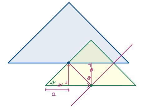
Figure 1. Triangles in $F_{a,A}$ in the proof of Theorem 14.

$\circleddash$ Step 3: Countable covering. We now show that we can cover the complementary of $C$ by a countable collection of the interior of such triangles, up to a remaining set $N\times\mathbb{R}$ having at most countable projections on the $t$-axis. Denoting by $\operatorname{r.i.}{}$ the relative interior of a set, define the open set

$$B=\left\{(t,x)\in[0,T]\times\mathbb{R}\quad|\quad\exists(t_{0},x_{0})\in[0,T]\times\mathbb{R}\ :\ (t,x)\in\operatorname{r.i.}\big{(}T(t_{0},x_{0})\big{)}\right\}$$

Of course, since $B$ is open, it can be covered by a countable collection $\{\text{int}(T_{j})\}_{j\in\mathbb{N}}$ of the interiors of triangles $T_{j}=T(x_{j},y_{j})$, for $j\in\mathbb{N}$. Points outside of $B$, naturally, do not belong to the relative interior of any triangle (3.5), whatever point $(t_{0},x_{0})\notin C$ we choose; if it is outside of $C$, it could still serve as the ’center’ of such triangles. We now assert that $[0,T]\times\mathbb{R}\setminus(B\cup C)$ has at most a countable projection onto the $t$-axis, and we show it.

Let indeed $a,A>0$ and consider the set of points

$$F_{a,A}=\left\{(\tau,\xi)\notin C\quad|\quad b_{0}(\tau,\xi)\geq 2a\quad\wedge\quad(\tau,\xi)\notin\operatorname{r.i.}\big{(}T(t,x)\big{)}\quad\text{whenever $b_{0}(t,x)\geq a$}\right\}\ .$$

By properties of triangles isosceles, with equal angles $\arctan\bar{\eta}$, two points $(\tau_{1},\xi_{1})$ and $(\tau_{2},\xi_{2})$ belonging to $F_{a,A}$ with $\tau_{1}\neq\tau_{2}$ must have distance at least $a\sqrt{1+\bar{\eta}^{2}}$ just because both $(\tau_{1},\xi_{1})\notin T(\tau_{2},\xi_{2})$ and $(\tau_{2},\xi_{2})\notin T(\tau_{1},\xi_{1})$. See Fig. 1. In particular, each set $F_{a,A}$ has finite projection on the $t$-axis. Of course this proves the claim being

$$[0,T]\times\mathbb{R}\setminus\left(B\cup C\right)\subseteq\bigcup_{n\in\mathbb{N}}F_{2^{-n},n}$$

We thus get

$$[0,T]\times\mathbb{R}=B\bigcup C\bigcup N\times\mathbb{R}\qquad\text{with $N\subset[0,T]$ at most countable and $B=\bigcup_{j\in\mathbb{N}}T_{j}$.}$$

$\circleddash$ Step 4: Thesis on each triangle. By the finite speed of propagation, in any fixed triangle $T_{j}$ like in (3.5) the function $u$ is equal to the solution to

$$\begin{cases}w_{t}+f(w)_{x}=g(t,x,w)\,,\\ w(0,x)=\begin{cases}u(t_{0},x)&\left\lvert x-x_{0}\right\rvert\leq\widetilde{b}_{0}\\ \frac{1}{2\widetilde{b}_{0}}\int_{x_{0}-\widetilde{b}_{0}}^{x_{0}+\widetilde{b}_{0}}u(t_{0},y)dy&\left\lvert x-x_{0}\right\rvert>\widetilde{b}_{0}\end{cases}\,.\end{cases}$$

By the Tame Oscillation condition, see [Ch2, Lemma 2.3] jointly with [ACM1, Theorem 4.4], the inequality (3.6) holds also for the whole range of $w$: in particular, $D_{x}u(t,\cdot)\cdot\widetilde{r}_{i}(u(t,\cdot)$ is $\mathrm{SBV}_{\mathrm{loc}}$ outside an at most countable set $N_{j}$ of times by Theorem 9. As a consequence, ${{\mathfrak{\upsilon}}}_{i}^{\mathrm{Cantor}}(\tau)$ vanishes on $T_{j}$ whenever $\tau\notin N_{j}$, so that

(3.7) $$\left\lvert\left[D_{x}^{\mathrm{Cantor}}\lambda_{i}(u(\tau))\right]_{i}\right\rvert(T)\leq\int_{T_{\tau}}\left\lvert\nabla\lambda_{i}(u(\tau,x^{-}))\cdot r_{i}(u(\tau,x))\right\rvert\,\left\lvert{{\mathfrak{\upsilon}}}_{i}^{\mathrm{Cantor}}(\tau,dx)\right\rvert=0\qquad\text{if }\tau\notin N_{j}\ .$$

$\circleddash$ Step 5: Conclusion. Whenever $\tau\notin N$ the complementary of $C_{\tau}$ is covered by $\{T_{j}\}_{j\in\mathbb{N}}$, so that

$$\left\lvert\left[D_{x}^{\mathrm{Cantor}}\lambda_{i}(u(\tau))\right]_{i}\right\rvert(\mathbb{R})\leq\left\lvert\left[D_{x}^{\mathrm{cont}}\lambda_{i}(u)\right]_{i}\right\rvert(C_{\tau})+\left\lvert\left[D_{x}^{\mathrm{Cantor}}\lambda_{i}(u)\right]_{i}\right\rvert\left(\bigcup_{j\in\mathbb{N}}T_{j}\right)\stackrel{{\scriptstyle\eqref{E:snfwknjknr},\eqref{E:snfwknjknr2}}}{{=}}0\qquad\text{if }\tau\notin N\cup\bigcup_{j\in N}N_{j}\ .$$

We also conclude that the closed set $K^{*}=[0,T]\times\mathbb{R}\setminus\cup_{j\in\mathbb{N}}\{T_{j}\}\subset C$ almost satisfies the first part of the statement: by inner and outer regularity of the measures $D^{\mathrm{Cantor}}{{\mathfrak{\upsilon}}}_{i}$, $i=1,\dots,N$, we can pick-up a $\sigma$-compact subset $K$ of $K^{*}$ such that both $D_{x}^{\mathrm{jump}}(K)=0$ and

$$\sum_{i=1}^{n}D^{\mathrm{Cantor}}{{\mathfrak{\upsilon}}}_{i}(\mathbb{R}^{2}\setminus K)=\sum_{i=1}^{n}D^{\mathrm{Cantor}}{{\mathfrak{\upsilon}}}_{i}(\cup_{j\in\mathbb{N}}\{T_{j}\})=0\,.$$

∎

For a counterexample concerning that $\mathrm{SBV}$-regularity in this context might fail for $\lambda_{i}(u)$, as well as for $u$, we refer to Remark 7.2 in [BYTrieste], that we repeat here for completeness. Of course, it stays true also with source terms.

Example 17 ([BYTrieste]).

Consider

$$\begin{cases}u_{t}=0\\ {{\mathfrak{\upsilon}}}_{t}+\left((1+v+u)v\right)_{x}=0\end{cases}\qquad A(U)=Jf(U)=\begin{pmatrix}0&0\\ v&1+2v+u\end{pmatrix}\qquad U=\binom{u}{v}$$

Being a triangular system, with trivial first equation, of course $u(t)$ has a Cantor part for every $t>0$ whenever a Cantor part is present in $u(0)$. This is compatible with the statement: $\left[D^{\mathrm{Cantor}}_{x}\lambda_{2}(u,v)\right]_{2}\equiv 2D_{x}^{\mathrm{Cantor}}v$ must vanish, not $D_{x}^{\mathrm{Cantor}}\lambda_{2}(u,v)$, which indeed does not vanish if $u(0)$ has a Cantor part. We include details for clarity:

• eigenvalues:

  $$\lambda_{1}(u,v)=0 \lambda_{2}(u,v)=1+2v+u$$

  $$\nabla\lambda_{1}(u,v)=\begin{pmatrix}0\\ 0\end{pmatrix} \nabla\lambda_{2}(u,v)=\begin{pmatrix}1\\ 2\end{pmatrix}$$

• eigenvectors:

  $$\ell_{1}(u,v)=\binom{1}{0} r_{1}(u,v)=\frac{1}{(1+2v+u)^{2}+v^{2}}\begin{pmatrix}1+2v+u\\ -v\end{pmatrix}$$

  $$\ell_{2}(u,v)=\frac{1}{(1+2v+u)^{2}+v^{2}}\binom{v}{1+2v+u} r_{2}(u,v)=\begin{pmatrix}0\\ 1\end{pmatrix}$$

• derivatives:

  $$D_{x}^{\mathrm{Cantor}}\lambda_{1}(u,v)=0=\left[D^{\mathrm{Cantor}}_{x}\lambda_{1}(u,v)\right]_{1}=\left[D^{\mathrm{Cantor}}_{x}\lambda_{1}(u,v)\right]_{2}$$

  $$D_{x}^{\mathrm{Cantor}}\lambda_{2}(u,v)=1+2D_{x}^{\mathrm{Cantor}}v+D_{x}^{\mathrm{Cantor}}u$$

  which has components

  $$\left[D^{\mathrm{Cantor}}_{x}\lambda_{2}(u,v)\right]_{1}:= \left(\nabla\lambda_{2}(u,v)\cdot r_{2}(u,v)\right)\left(\ell_{1}(u,v)\cdot D_{x}^{\mathrm{Cantor}}(u,v)\right)\equiv 2D^{\mathrm{Cantor}}_{x}u$$

  $$\left[D^{\mathrm{Cantor}}_{x}\lambda_{2}(u,v)\right]_{2}:= \left(\nabla\lambda_{2}(u,v)\cdot r_{2}(u,v)\right)\left(\ell_{2}(u,v)\cdot D_{x}^{\mathrm{Cantor}}(u,v)\right)$$

  $$\equiv \frac{1}{(1+2v+u)^{2}+v^{2}}\left(vD_{x}^{\mathrm{Cantor}}u+(1+2v+u)D_{x}^{\mathrm{Cantor}}v\right)$$

The SBV-like regularity thus guarantees that $vD_{x}^{\mathrm{Cantor}}u+(1+2v+u)D_{x}^{\mathrm{Cantor}}v$ vanishes. Nevertheless, of course if a Cantor part is present at time $t=0$ in $D_{x}u$ it will be present also at all future times…

4. $\mathrm{SBV}$ regularity for generic, non-degenerate fluxes

The case of a genuinely nonlinear field of Theorem 9 might seem restrictive. Nevertheless, it is not merely the key step in order to get the $\mathrm{SBV}$ regularity of the entropy solutions when all fields are genuinely nonlinear as in [Lax], but also when they are piecewise genuinely nonlinear as in [IguchiLeFloch], and more generally when they satisfy the non-degeneracy condition introduced in [LeFlochGlasse], slightly different from the one we consider here. We believe it is important to include the $\mathrm{SBV}$-regularity under this last non-degeneracy condition because generic fluxes do satisfy such condition, so that they approximate any flux, see Remark 19 below.

Definition 18.

Let $\lambda_{1}\,,\dots\,,\lambda_{N}$ be the eigenvalues of a matrix $A\in C^{M}(\Omega)$, where $M\in\mathbb{N}\cup\{+\infty\}$ and $M\geq 2$. We consider $A$ non-degenerate if for all $i=1,\dots,N$ there holds

(4.1) $$\left\{\pi_{i}^{(k)}\right\}_{k=1,\dots,M}\neq 0^{M} \text{where }\pi_{i}^{(1)}=\nabla\lambda_{i}\cdot r_{i}\text{ and }\pi_{i}^{(k+1)}=\nabla\pi_{i}^{(k)}\cdot r_{i}\,,\ k=1,\dots,M-1\,.$$

In case of a scalar equation, when $N=1$, then $\pi_{1}^{(1)}=f^{\prime\prime}$ and $\pi_{1}^{(k)}=f^{(k+1)}$: a flux is called non-degenerate for us if there is a derivative higher than the first which is non-vanishing. In [LeFlochGlasse] $f$ was considered piecewise genuinely nonlinear if $f^{\prime\prime}$ and $f^{\prime\prime\prime}$ do not vanish simultaneously, and in [IguchiLeFloch] the same condition denoted non-genenerate fluxes.

Remark 19.

When all fields are genuinely nonlinear, then $\pi_{i}^{(1)}\neq 0$ for $i=1,\dots,N$ and this non-degeneracy condition holds. Piecewise genuinely nonlinear fluxes of [IguchiLeFloch] satisfy that $\pi_{i}^{(1)}$, $\pi_{i}^{(2)}$ do not vanish simultaneously, for $i=1,\dots,N$. In [LeFlochGlasse] fluxes were called non-degenerate when $\pi_{i}^{(1)}$, …, $\pi_{i}^{(N+1)}$ are non-vanishing simultaneously, for $i=1,\dots,N$. With the Whitney topology and when $M\geq N+1$, the set of functions $A\in C^{\infty}(\Omega)$ satisfying our non-degeneracy condition (4.1) contain the intersection of a countable number of open dense subsets by [LeFlochGlasse, § 2.6]: in particular, see [LeFlochGlasse, Theorem 2.13], the relative fluxes approximate any smooth flux in the Whitney topology.

Before relating the non-degeneracy of the flux to the regularity of solutions, we better understand the condition.

Lemma 20.

Suppose $A$ is non-degenerate as in Definition 18. For each $i=1,\dots,N$ and any $R>0$, the set

$$Z_{i}:=\{u\in\Omega\quad:\quad\nabla\lambda_{i}(u)\cdot r_{i}(u)=0\}\cap[-R,R]^{N}$$

is the union of finitely many disjoint smooth sub-manifolds $\{Z_{i}^{k}\}_{k=1}^{J_{i}}$ of dimension at most $N-1$, all transversal to $r_{i}$.

Proof.

Since the non-degeneracy assumption grants that $\pi^{(1)}_{i}$, …, $\pi^{(M)}_{i}$ do not vanish simultaneously, the decomposition can be constructed applying the implicit function theorem to the sets

$$\bigcap_{k=1}^{\ell}\{\pi^{(k)}_{i}=0\}\cap\{\pi^{(\ell+1)}_{i}\neq 0\}\qquad\text{for }\ell=M-1,\dots,1\,.$$

Consider now any $u\in Z_{i}$ and consider any smooth curve $\underline{\gamma}:(-1,1)\to Z_{i}$ with $\underline{\gamma}(0)=u$. In particular, for $|t|\leq 1$ one has $\pi^{(1)}_{i}(\underline{\gamma}(t))=0$ identically so that

$$\frac{d}{dt}\pi^{(k)}_{i}\circ\underline{\gamma}|_{t=0}=\nabla\pi^{(k)}_{i}(u)\cdot\dot{\underline{\gamma}}(0)=0\qquad\forall k\in\mathbb{N}\,.$$

By the non-degeneracy assumption, necessarily $\dot{\underline{\gamma}}(0)\neq r_{i}(u)$: being different from any direction tangent to $Z_{i}$, thus $r_{i}(u)$ must be transversal to $Z_{i}$. ∎

We now state the regularity result.

Theorem 21 ($\mathrm{SBV}$ regularity for non-degenerate systems).

Let $u\in\mathrm{BV}([0,T]\times\mathbb{R};\Omega)$ be an entropy solution of the strictly hyperbolic system of balance laws (1.1) with small $\mathrm{BV}$ norm. Suppose $g$ satisfies Assumption (G): at Page (G): and $A$ is nondegenerate in $\Omega$ as in (4.1). Then there exists an at most countable set $S\subset[0,T]$ of times such that $x\mapsto u(t,x)$ is a special function of bounded variation for every $t\in[0,T]\setminus S$. In particular, $u\in\mathrm{SBV}([0,T]\times\mathbb{R})$.

Before entering the proof, we give a general auxiliary lemma in real analysis.

Lemma 22.

Consider a function $w:\mathbb{R}\to\mathbb{R}^{N}$ with bounded variation and let $K\subset\mathbb{R}$ be a compact set of continuity points of $w$ with $\left|D_{x}^{\mathrm{Cantor}}w\right|(K)>0$ and $w(K)\subset\{x_{1}=0\}$. Then $\mathrm{e}_{1}\cdot D_{x}^{\mathrm{Cantor}}w\restriction_{K}=0$.

Proof.

One can as well assume that $\mathcal{L}^{1}(K)=0$, since the Cantor part of $D_{x}w$ is singular with respect to the Lebesgue measure. Suppose also that $K$ is compact, by inner regularity of measures. Let $\varepsilon>0$. Cover $K$ with open intevals $(a_{1},b_{1})$, …, $(a_{J},b_{J})$ with $b_{i}<a_{k}$ if $i<k$ and such that

(4.2) $$\sum_{i=1}^{J}(b_{i}-a_{i})\leq\varepsilon\,,\qquad\left|D_{x}w\right|\left(\bigcup_{i=1}^{J}(a_{i},b_{i})\setminus K\right)<\varepsilon\,.$$

If $\overline{a}_{i}$ is the closest point to $a_{i}$ in $K\cap(a_{i},b_{i})$, $\overline{b}_{i}$ the closest to $b_{i}$, then $K\subset\cup_{i=1}^{J}[\overline{a}_{i},\overline{b}_{i}]$ and $\sum_{i=1}^{J}(\overline{b}_{i}-\overline{a}_{i})\leq\varepsilon$. Since by hypothesis $w(J)\subset\{x_{1}=0\}$, in particular $w(\overline{a}_{i})\subset\{x_{1}=0\}$ and $w(\overline{b}_{i})\subset\{x_{1}=0\}$ for $i=1,\dots,J$.

Consider in $[\overline{a}_{1},\overline{b}_{J}]$ the auxiliary function

$$w_{\varepsilon}=w-\int_{\overline{a}_{1}}^{x}D_{x}w\restriction_{\cup_{i=1}^{J-1}[\overline{b}_{i},\overline{a}_{i+1}]}=w(\overline{a}_{1})+\int_{\overline{a}_{1}}^{x}D_{x}w\restriction_{\cup_{i=1}^{J}[\overline{a}_{i},\overline{b}_{i}]}\,.$$

In particular

(4.3) $$D_{x}w_{\varepsilon}\restriction_{\cup_{i=1}^{J}[\overline{a}_{i},\overline{b}_{i}]}=D_{x}w\restriction_{\cup_{i=1}^{J}[\overline{a}_{i},\overline{b}_{i}]}\quad\text{and}\quad D_{x}w_{\varepsilon}\restriction_{\cup_{i=1}^{J-1}[\overline{b}_{i},\overline{a}_{i+1}]}=0\,.$$

Since $w(\overline{a}_{i}),w(\overline{b}_{i})\in\{x_{1}=0\}$, then for $i=1,\dots,J$ one has

(4.4) $$0=(w(\overline{b}_{i})-w(\overline{a}_{i}))\cdot\mathrm{e}_{1}=\left(\int_{\overline{a}_{i}}^{{\overline{b}_{i}}}Dw(x)\,dx\right)\cdot\mathrm{e}_{1}\quad\Rightarrow\quad(w_{\varepsilon}(\overline{b}_{i})-w_{\varepsilon}(\overline{a}_{i}))\cdot\mathrm{e}_{1}=0\,.$$

Considering that $w_{\varepsilon}(\overline{a}_{1})=w(\overline{a}_{1})\in\{x_{1}=0\}$, then $w_{\varepsilon}(\overline{b}_{1})\in\{x_{1}=0\}$.

If $\overline{b}_{i}\leq x\leq\overline{a}_{i+1}$, then $w_{\varepsilon}(x)=w_{\varepsilon}(\overline{b}_{i})$ so that $w_{\varepsilon}(x)\in\{x_{1}=0\}$ in $[\overline{b}_{1},\overline{a}_{2}]$. Going on iteratively by (4.4), this yields $w_{\varepsilon}(x)\in\{x_{1}=0\}$ in each $[\overline{b}_{i},\overline{a}_{i+1}]$, $i=1,\dots J-1$.

If $x\in(\overline{a}_{i},\overline{b}_{i})\setminus K$ then $w_{\varepsilon}(x)\in\{|x_{1}|\leq\varepsilon\}$ because

$$\left\lvert w_{\varepsilon}(x)-w_{\varepsilon}(\overline{a}_{i})\right\rvert\leq\left\lvert D_{x}w_{\varepsilon}\right\rvert\left((a_{i},b_{i})\setminus K\right)\stackrel{{\scriptstyle\eqref{E:ggrgrgr}}}{{=}}\left\lvert D_{x}w\right\rvert\left((a_{i},b_{i})\setminus K\right)\stackrel{{\scriptstyle{\eqref{E:approxCantor}}}}{{\leq}}\varepsilon\,.$$

As $\varepsilon\downarrow 0$ we can require $I_{\varepsilon}=\cup_{i=1}^{J-1}[\overline{b}_{i},\overline{a}_{i+1}]$ decreasing and $w_{\varepsilon}$ converges to $\widehat{w}(x)=\int_{a_{1}}^{x}D^{\mathrm{Cantor}}_{x}w\restriction_{K}$, thus valued in $\{x_{1}=0\}$, the convergence is also uniform. Since $\widehat{w}\cdot\mathrm{e}_{1}=0$ identically, we thus arrive to the thesis

$$0=D_{x}(\widehat{w}\cdot\mathrm{e}_{1})=(D_{x}\widehat{w})\cdot\mathrm{e}_{1}=(D_{x}^{\mathrm{Cantor}}w)\cdot\mathrm{e}_{1}\,.\qed$$

Corollary 23.

Let $Z\subset\mathbb{R}^{N}$ be a smooth manifold with codimension at least $1$ and with any normal direction $\hat{n}$. Consider a function $w:\mathbb{R}\to\mathbb{R}^{N}$ with bounded variation and let $K\subset\mathbb{R}$ be a $\sigma$-compact set of continuity points of $w$ with $\left|D_{x}^{\mathrm{Cantor}}w\right|(K)>0$ and $w(K)\subset Z$. Then $\hat{n}\cdot D_{x}^{\mathrm{Cantor}}w\restriction_{K}=0$, which implies, applying this repeatedly with different $\hat{n}$, that $D_{x}^{\mathrm{Cantor}}w\restriction_{K}$ is tangent to $Z$.

Proof.

If the dimension of $Z$ is less than $N-1$, just extend $Z$ to a bigger one which still has $\hat{n}$ has a normal direction: we thus consider only the case of dimension $N-1$.

Focus on a small neighborhood of a point, for example of the origin. Once parametrized there the surface smoothly as $\{\sigma(x_{2},\dots,x_{N})\ :\ (x_{2},\dots,x_{N})\in B_{\delta}(0)\}$ with $\sigma$ one-to-one, consider the function

$$\widehat{w}=\sigma^{-1}\circ w:\mathbb{R}\to\{x_{1}=0\}\subset\mathbb{R}^{N}\,.$$

By Volpert chain rule, $\widehat{w}\in\mathrm{BV}(\mathbb{R};\mathbb{R}^{N})$ and $D_{x}^{\mathrm{Cantor}}\widehat{w}=J\sigma^{-1}(w)\cdot D_{x}^{\mathrm{Cantor}}w$, equivalent to

(4.5) $$D_{x}^{\mathrm{Cantor}}w=J\sigma(\widehat{w})\cdot D_{x}^{\mathrm{Cantor}}\widehat{w}\,.$$

Since the tangent plane to $Z$ is generated by $\partial_{x_{2}}\sigma$, …, $\partial_{x_{N}}\sigma$ and $D_{x}^{\mathrm{Cantor}}\widehat{w}$ is a linear combination of $\mathrm{e}_{2}$, …, $\mathrm{e}_{N}$ by Lemma 22, we get from (4.5) that $D_{x}^{\mathrm{Cantor}}w$ is a linear combination of $\partial_{x_{2}}\sigma$, …, $\partial_{x_{N}}\sigma$ thus tangent to $Z$. ∎

We now give an auxiliary lemma related to balance laws.

Lemma 24.

Under the hypothesis of Theorem 21, set $w(x)=u(t,x)$. Consider a compact set $K\subseteq\mathbb{R}$ of continuity points of $w$ with $\mathcal{L}^{1}(K)=0$. If there are $X\subseteq\{1,\dots,N\}$ and $\{k_{i}\}_{i\in X}$ with $w(x)\in Z_{i}^{k}$ precisely if $i\in X$ and $k=k_{i}$, then $D_{x}^{\mathrm{Cantor}}w{\restriction_{K}}$ vanishes.

Proof of Lemma 24.

We can decompose $D_{x}^{\mathrm{Cantor}}u{\restriction_{K}}$ along the right eigenvectors $r_{i}$ as in Definition 7, where we introduced the wave measures ${{\mathfrak{\upsilon}}}_{i}$. Since $\nabla\lambda_{i}(u)\cdot r_{i}(u)\neq 0$ for $i\notin K$, Theorem 14 ensures that $D^{\mathrm{Cantor}}{{\mathfrak{\upsilon}}}_{i}\restriction_{K}$ vanish when $i\notin X$. We can therefore write:

(4.6) $$D_{x}^{\mathrm{Cantor}}w{\restriction_{K}}=\sum_{i\in X}{{{\mathfrak{\upsilon}}}_{i}}r_{i}(w)\qquad\text{where ${{{\mathfrak{\upsilon}}}_{i}}:=D_{x}^{\mathrm{Cantor}}w{\restriction_{K}}\cdot\ell_{i}(w)$.}$$

By Corollary 23, if $K$ satisfying (1-3) exists then $D_{x}^{\mathrm{Cantor}}w$ must be tangent to each $Z_{i}^{j_{i}}$, $i\in X$: by Lemma 20 it must be thus transversal to each $r_{i}$ for $i\in X$. Add to $\{r_{i}\}_{i\in X}$ vectors $b_{1},\dots,b_{N-\sharp X}$ to obtain a basis of $\mathbb{R}^{N}$ and such that the tangent plane to the intersection $\cap_{i\in X}Z_{i}$ is contained in $\langle b_{1},\dots,b_{N-\sharp X}\rangle$: we decompose $D_{x}w{\restriction_{K}}$ along the vectos $b_{1},\dots,b_{N-\sharp X}$ and we write

(4.7) $$D_{x}^{\mathrm{Cantor}}w{\restriction_{K}}=\sum_{i\notin X}\widehat{{{\mathfrak{\upsilon}}}_{i}}b_{i}(w)\qquad\text{where $\widehat{{{\mathfrak{\upsilon}}}_{i}}:=D_{x}^{\mathrm{Cantor}}w{\restriction_{K}}\cdot r_{i}(w)$.}$$

Jointly with (4.6), we conclude that $D_{x}^{\mathrm{Cantor}}w{\restriction_{K}}$ vanishes because $\langle r_{i}\rangle_{i\in X}$ and $\langle b_{i}\rangle_{i\notin X}$ are transversal: the system

$$0=b_{k}(w)\cdot D_{x}^{\mathrm{Cantor}}w{\restriction_{K}}=b_{k}(w)\cdot\sum_{i\in X}{{{\mathfrak{\upsilon}}}_{i}}r_{i}(w)=\sum_{i\in X}{{{\mathfrak{\upsilon}}}_{i}}\langle b_{k}(w)\,,r_{i}(w)\rangle\qquad k\notin X$$

$$0=r_{k}(w)\cdot D_{x}^{\mathrm{Cantor}}w{\restriction_{K}}=r_{k}(w)\cdot\sum_{i\notin X}\widehat{{{\mathfrak{\upsilon}}}_{i}}b_{i}(w)=\sum_{i\notin X}\widehat{{{\mathfrak{\upsilon}}}_{i}}\langle b_{k}(w)\,,r_{i}(w)\rangle\qquad k\in X$$

by its invertibility implies ${{{\mathfrak{\upsilon}}}_{i}}=\widehat{{{\mathfrak{\upsilon}}}_{i}}=0$ for $i=1,\dots,N$. ∎

Proof of Theorem 21.

In the proof of Theorem 14, the strip $[0,T]\times\mathbb{R}$ was covered with

• at most countably many exceptional time-lines $\{t_{k}\}\times\mathbb{R}$, $k\in\mathbb{N}$, $0\leq t_{k}\leq T$,

• a jump set $J$, whose section $J_{\tau}=J\cap\{\tau\}\times\mathbb{R}$ is at most countable for all $0\leq\tau\leq T$,

• a countable union $B$ if open triangles where $u$ is a special function of bouded variation,

• the inverse images $u^{-1}(Z_{i}^{j})$, $j=1,\dots,J_{i}$, of the manifolds of Lemma 20 transversal to $r_{i}$ where $\nabla\lambda_{i}\cdot r_{i}=0$.

Consider any time $\overline{t}\notin\{t_{k}\}_{k\in\mathbb{N}}$. Consider any compact set $K\subseteq\mathbb{R}$ of continuity points of $w(x)\doteq u(\overline{t},x)$ that satisfies $\mathcal{L}^{1}(K)=0$. For each $X\subset\{1,\dots,N\}$ and any selection $\{j_{i}\}$ one has that $D_{x}^{\mathrm{Cantor}}w{\restriction_{K}}\cap u^{-1}(\{Z_{i}^{j_{i}}\}_{i\in X})$ vanishes by Lemma 24 jointly with $\sigma$-additivity. By $\sigma$-additivity and by inner regularity of measures, the Cantor part of $D_{x}u(\overline{t})$ must thus vanish. Because of the slicing theory of $\mathrm{BV}$-functions (2.4) then the Cantor part of $D_{x}u$ must thus vanish, as the Cantor part of the derivative of the time restrictions vanishes at almost every time. ∎

Appendix A An account on the solution to the Cauchy problem

In this section we describe the main ingredients in order to construct a piecewise constant approximation of a solution $u$ to Eqs. (1.1)-(1.2), first in the homogeneous case $g=0$ then in the non homogeneous case.

We begin in § A.1 summarising the construction of the self-similar solution to conservation laws with the Riemann problem, which is when the datum has single jump in the origin.

This allows then to describe in § A.2 an algorithm for defining piecewise-constant approximations first to the Cauchy problem for a conservation law, in particular the front-tracing solution, then paring it with an operator splitting method, to the Cauchy problem for a balance law.

In turn, in § A.3 we review the functionals that provide estimates needed for compactness, precisely the interaction estimates, that play an important point also the in the estimates to obtain $\mathrm{SBV}$-regularity.

Finally, in § A.4 we remind the convergence result of the approximation constucted.

A.1. The nonconservative Riemann problem

Since we deal with a system that, in general, it is not in conservation form, we briefly recall the construction of the solution to a Riemann problem in the homogeneous case, i.e.

(A.1a) $$u_{t}+A(u)u_{x}=0$$

(A.1b) $$u(0,x)=\begin{cases}u^{L}\quad&\text{if\quad$x<0$\,,}\\ u^{R}\quad&\text{if\quad$x>0$\,.}\end{cases}$$

We refer to [BB, srp] for the details.

As in the Introduction, we let $A$ be a smooth matrix-valued map, with eigenvalues given by Equation  (1.4b), and right and left eigenvalues as in Eqs. (1.5)-(1.6). Since we are interested in solutions to Equation  (1.1) with small total variation, it is not restrictive to assume that there exist constants $\widehat{\lambda}_{0}<\cdots<\widehat{\lambda}_{N}$ such that

(A.2) $$\widehat{\lambda}_{k-1}<\lambda_{k}(u)<\widehat{\lambda}_{k}\,,\qquad\forall~{}u\,,\quad k=1,\dots,N\,.$$

Given any continuous function $f:I\subset\to$, and any interval $[a,b]\subset I$, we will denote the lower convex envelope and the upper concave envelope of $f$ on $[a,b]$, respectively, as

(A.3) $$\mathop{\rm conv}\nolimits_{[a,b]}f(x)\doteq\inf\Big{\{}\theta f(y)+(1-\theta)f(z):\theta\in[0,1]\,,\ y,z\in[a,b]\,,\ x=\theta y+(1-\theta)z\Big{\}}\,,$$

and

(A.4) $$\mathop{\rm conc}\nolimits_{[a,b]}f(x)\doteq\sup\Big{\{}\theta f(y)+(1-\theta)f(z):\theta\in[0,1]\,,\ y,z\in[a,b]\,,\ x=\theta y+(1-\theta)z\Big{\}}\,.$$

We will simply write $\mathop{\rm conv}\nolimits f,\,\mathop{\rm conc}\nolimits f$, whenever there is no ambiguity on the interval $[a,b]$ taken in consideration. As usual, in order to construct a solution to Equation  (A.1), the basic step consists in constructing the elementary curve of the $k$-th family $(k=1,\dots,N)$ for every given left state $u^{L}$, which is a one parameter curve of right states $s\mapsto T_{k}[u^{L}](s)$ with the property that the Riemann problem having initial data $(u^{L},u^{R})$, $u^{R}\doteq T_{k}[u^{L}](s)$, admits a vanishing viscosity solution consisting only of waves of the $k$-th characteristic family. In order to construct such a curve, we look for traveling waves solutions to the parabolic system

(A.5) $$u_{t}+A(u)u_{x}=u_{xx}\,,$$

solutions to Equation  (A.5) of the form $u(t,x)=\phi(x-\sigma\,t)$, for some constant $\sigma$. The profile $\phi$ satisfies the second order ODE

$$\big{(}A(\phi)-\sigma\big{)}\,\phi^{\prime}=\phi^{\prime\prime}\,,$$

which can be written as a first order system of ODEs on the space ${}^{N}\times^{N}\times$:

(A.6) $$\begin{cases}\dot{u}=v\,,\\ \dot{v}=\big{(}A(\phi)-\sigma\big{)}\,v\,,\\ \dot{\sigma}=0\,.\end{cases}$$

Applying the Center Manifold Theorem, we get that in a neighborhood of a given equilibrium point $(u_{0},\,0,\,\lambda_{k}(u_{0}))\in^{N}\times\times$ for Equation  (A.6) there exists an $N+2$-dimensional center manifold $\mathcal{M}_{k}$ which is locally invariant under the flow of (A.6). Introducing the coordinates

$$v_{h}\doteq{\big{\langle}l_{h}(u_{0}),v\big{\rangle}}\,,\qquad\quad h=1,\dots,N\,,$$

of a vector $v\in^{N}$ relative to the basis $r_{1}(u_{0}),\dots$ $\dots,r_{N}(u_{0})$, one can parameterize $\mathcal{M}_{k}$ in terms of the variables $u,\,v_{k},\,\sigma$, namely

$$\mathcal{M}_{k}=\big{\{}(u,v,\sigma)~{};~{}~{}v=v_{k}\,\widetilde{r}_{k}(u,v_{k},\sigma)\big{\}}$$

for suitable smooth vector functions $(u,v_{k},\sigma)\mapsto\widetilde{r}_{k}(u,v_{k},\sigma)$ defined on a neighborhood of $(u_{0},0,\lambda_{k}(u_{0}))$, that satisfy

$$\widetilde{r}_{k}\big{(}u_{0},0,\sigma\big{)}=r_{k}(u_{0})\qquad\forall~{}\sigma\,,$$

and are normalized so that

(A.7) $${\big{\langle}l_{k}(u_{0}),\widetilde{r}_{k}(u,v_{k},\sigma)\big{\rangle}}=1\qquad\forall~{}u\,,\,v_{k}\,,\,\sigma\,.$$

By construction, $\mathcal{M}_{k}$ contains all bounded viscous traveling profiles with speed close to $\lambda_{k}(u_{0})$. Thus, we can rewrite the linearized equations for (A.6) at $(u_{0},0,\lambda_{k}(u_{0}))$ on the manifold $\mathcal{M}_{k}$, and obtain a system on the space ${}^{N}\times\times$:

(A.8) $$\begin{cases}u_{x}=v_{k}\widetilde{r}_{k}(u,v_{k},\sigma)\,,\\ v_{k,x}=v_{k}\big{(}\,\widetilde{\lambda}_{k}(u,v_{k},\sigma)-\sigma\,\big{)}\,,\\ \sigma_{x}=0\,,\end{cases}$$

where

(A.9) $$\widetilde{\lambda}_{k}(u,v_{k},\sigma)\doteq{\big{\langle}l_{k}(u),A(u)\,\widetilde{r}_{k}(u,v_{k},\sigma)\big{\rangle}}\,.$$

Because of the normalization (A.7), the smooth scalar function $(u,v_{k},\sigma)\mapsto\widetilde{\lambda}_{k}(u,v_{k},\sigma)$ satisfies the identity

(A.10) $$\widetilde{\lambda}_{k}\big{(}u_{0},v_{k},\sigma\big{)}=\lambda_{k}(u_{0})\qquad\forall~{}v_{k}\,,\,\sigma\,.$$

Next, given a left state $u^{L}$ in a neighborhood of $u_{0}$ and $0<s<<1$, in connection with the equations (A.8) describing the evolution of traveling profiles on the manifold $\mathcal{M}_{k}$ we associate the integral system

(A.11) $$\begin{cases}u(\tau)=u^{L}+\displaystyle{\int_{0}^{\tau}}\widetilde{r}_{k}\big{(}u(\xi),v_{k}(\xi),\sigma(\xi)\big{)}~{}d\xi\,,\\ \vskip 6.0pt plus 2.0pt minus 2.0pt\cr v_{k}(\tau)=\widetilde{F}_{k}\big{(}\tau;\,u,v_{k},\sigma\big{)}-\mathop{\rm conv}\nolimits_{[0,s]}\widetilde{F}_{k}\big{(}\tau;\,u,v_{k},\sigma\big{)}\,,\\ \vskip 6.0pt plus 2.0pt minus 2.0pt\cr\sigma(\tau)=\displaystyle{\frac{d}{d\tau}}\mathop{\rm conv}\nolimits_{[0,s]}\widetilde{F}_{k}\big{(}\tau;\,u,v_{k},\sigma\big{)}\,,\end{cases}\qquad 0\leq\tau\leq s\,,$$

where $\tau\mapsto\widetilde{F}_{k}(\tau;\,u,v_{k},\sigma)$ is the “reduced flux function” associated to (1.13) defined, by

(A.12) $$\widetilde{F}_{k}(\tau;\,u,v_{k},\sigma)\doteq\int_{0}^{\tau}\widetilde{\lambda}_{k}\big{(}u(\xi),v_{k}(\xi),\sigma(\xi)\big{)}~{}d\xi\,.$$

In [BB] it is shown that, for $s$ sufficiently small, the transformation defined by the right-hand side of (A.11) maps a domain of continuous curves $\tau\mapsto(u(\tau),v_{k}(\tau),\sigma(\tau))$ into itself, and is a contraction w.r.t. a suitable weighted norm. Hence, for every $u^{L}$ in a neighborhood $\mathcal{U}_{0}$ of $u_{0}$, the transformation defined by (A.11) admits a unique fixed point

(A.13) $$\tau\mapsto\big{(}\overline{u}(\tau;\,u^{L},s),\ \overline{v}_{k}(\tau;\,u^{L},s),\ \overline{\sigma}(\tau;\,u^{L},s)\big{)}\qquad\tau\in[0,s]\,,$$

which provides a Lipschitz continuous solution to the integral system (A.11). The elementary curve of right states of the $k$-th family issuing from $u^{L}$ is then defined as the terminal value at $\tau=s$ of the $u$-component of the solution to the integral system (A.11), i.e. by setting

(A.14) $$T_{k}[u^{L}](s)\doteq u(s;\,u^{L},s)\,.$$

For the sake of convenience, we denote

(A.15) $$\sigma_{k}[u^{L}](s,\tau) \doteq\sigma(\tau;\,u^{L},s)\,,$$

$$\widetilde{F}_{k}[u^{L}](s,\tau) \doteq\widetilde{F}_{k}\big{(}\tau;u(\cdot\ ;u^{L},s),v_{k}(\cdot;u^{L},s),\sigma(\cdot;u^{L},s)\big{)}$$

For negative values $s<0$, $|s|<<1,$ one replaces in (A.11) the lower convex envelope of $\widetilde{F}_{k}$ on the interval $[0,s]$ with its upper concave envelope on $[s,0]$, and then constructs the curve $T_{k}[u^{L}]$ and the map $\sigma_{k}[u^{L}]$ exactly in the same way as above looking at the solution of the integral system (A.11) on the interval $[s,0]$. In such a way, given any pair of states $u^{L},u^{R}$ with $|u^{L}-u_{0}|,|u^{R}-u_{0}|<<1$, if $u^{R}=T_{k}[u^{L}](s)$, for some wave size $s$, then the self-similar solution to the Riemann problem with initial data $(u^{L},u^{R})$, determined by the vanishing viscosity approximation in Equation  (1.3) as $\varepsilon\to 0+$, is given by the piecewise continuous function

(A.16) $$u(t,x)=\begin{cases}u^{L}\quad&\text{if\quad$x/t<\sigma_{k}[u^{L}](s,\,0)\,,$}\\ \vskip 3.0pt plus 1.0pt minus 1.0pt\cr T_{k}[u^{L}](\tau)\quad&\text{if\quad$x/t=\sigma_{k}[u^{L}](s,\,\tau)$ \quad for some $\tau\in\mathcal{I}$\,,}\\ \vskip 3.0pt plus 1.0pt minus 1.0pt\cr u^{R}\quad&\text{if\quad$x/t>\sigma_{k}[u^{L}](s,\,s)\,,$}\end{cases}$$

Remark 25.

If the system (1.1) is in conservation form, i.e. in the case where $A(u)=DF(u)$ for some smooth flux function $F$, the general solution of the Riemann problem provided by (A.16) is a composed wave of the $k$-th family containing a countable number of rarefaction waves and contact-discontinuities or compressive shocks which satisfy the Liu admissibility condition [tplrp2p2, tplrpnpn]. Namely, the regions where the $v_{k}$-component of the solution to (A.11) vanishes correspond to rarefaction waves if the $\sigma$-component is strictly increasing and to contact discontinuities if the $\sigma$-component is constant, while the regions where the $v_{k}$-component of the solution to (A.11) is different from zero correspond to compressive shocks.

In view of the considerations of Remark 25, we will extend the standard terminology adopted for the elementary waves that are present in the solution of an hyperbolic system of conservation laws to the general case of non conservative systems. Thus, we will say that any (vanishing viscosity) solution of the Riemann problem for (1.1) of the form (A.16) is a centered rarefaction wave of the $k$-th family whenever $u^{R}\in R_{k}[u^{L}](s)$ for some wave size $s$ such that $\tau\mapsto\sigma_{k}[u^{L}](s,\tau)$ be strictly increasing on $[0,s]$, $s>0$ (or strictly decreasing on $[s,0]$ if $s<0$), while we will say that any (vanishing viscosity) solution of a Riemann problem for (1.1) of the form

$$u(t,x)=\begin{cases}u^{L}\quad&\text{if\quad$x<\lambda t$\,,}\\ u^{R}\quad&\text{if\quad$x>\lambda t$\,,}\end{cases}$$

is an admissible shock wave of the $k$-th family when $u^{R}=T_{k}[u^{L}](s)$ and $\sigma_{k}[u^{L}](s,0)=\sigma_{k}[u^{L}](s,s)=\lambda$. Once we have constructed the elementary curves $T_{k}$ for each $k$-th characteristic family, the vanishing viscosity solution of a general Riemann problem for (1.1) is then obtained by a standard procedure observing that the composite mapping

(A.17) $$\Phi(s_{1},\dots,s_{N})[u^{L}]\doteq T_{N}\Big{[}T_{N-1}\Big{[}\cdots\big{[}T_{1}[u^{L}](s_{1})\big{]}\cdots\Big{]}(s_{N-1})\Big{]}(s_{N})\doteq u^{R}\,,$$

is one-to-one from a neighborhood of the origin onto a neighborhood of $u^{L}$. This is a consequence of the fact that the curves $T_{k}[u]$ are tangent to $r_{k}(u)$ at zero $s=0$ [BB, srp]. Therefore, we can uniquely determine intermediate states $u^{L}\doteq\omega_{0},$ $\omega_{1},$ $\dots,$ $\omega_{N}\doteq u^{R}$, and wave sizes $s_{1},\dots,s_{N},$ such that there holds

(A.18) $$\omega_{k}=T_{k}[\omega_{k-1}](s_{k})\quad\qquad k=1,\dots,N\,,$$

provided that the left and right states $u^{L},u^{R}$ are sufficiently close to each other. Each Riemann problem with initial data

(A.19) $$\overline{u}_{k}(x)=\begin{cases}\omega_{k-1}&\text{if \ \ $x<0$,}\\ \omega_{k}&\text{if \ \ $x>0$,}\end{cases}$$

admits a vanishing viscosity solution of total size $s_{k}$, containing a sequence of rarefactions and Liu admissible discontinuities of the $k$-th family. Then, because of the uniform strict hyperbolicity assumption (A.2), the general solution of the Riemann Problem with initial data $\big{(}u^{L},\,u^{R}\big{)}$ is obtained by piecing together the vanishing viscosity solutions of the elementary Riemann problems (1.1) (A.19). Throughout the paper, with a slight abuse of notation, we shall often call $s$ a wave of (total) size $s$, and, if $u^{R}=T_{k}[u^{L}](s)$, we will say that $(u^{L},\,u^{R})$ is a wave of size $s$ of the $k$-th characteristic family.

A.2. The algorithm

Now we briefly describe the algorithm we use in order to construct a piecewise constant approximate solution to Eqs. (1.1)-(1.2). First of all let us recall what a front tracking solution to an homogeneous hyperbolic system is (see [AMfr] for details).

Definition 26.

Let $\varepsilon>0$ and an interval $I\subset\mathbb{R}$ be fixed, and let $A=A(u)$, $u\in\mathbb{R}^{N}$, be a smooth hyperbolic $N\times N$ matrix. We say that a continuous map $u:I\mapsto{\mathbb{L}^{1}}_{loc}(;\,^{N})$, is an $\varepsilon$-approximate front tracking solution to Equation  (A.1a) if the following conditions hold:

1. As a function of two variables, $u=u(t,x)$ is piecewise constant with discontinuities occurring along finitely many straight lines in the $t$-$x$ plane. Jumps can be of two types: elementary wave-fronts and nonphysical wave-fronts, denoted, respectively, as $\mathcal{E}$ and $\mathcal{NP}$. Only finitely many wave-fronts interactions occur, each involving exactly two incoming fronts.

2. Along each elementary front $x=x_{\alpha}(t)$, $\alpha\in\mathcal{E}$, the values $u^{L}\doteq u(t,\,x_{\alpha}-)$ and $u^{R}\doteq u(t,\,x_{\alpha}+)$ satisfy the following properties. There exists some wave size $s_{\alpha}$ and some index $k_{\alpha}\in\{1,\dots,N\}$ such that

   (A.20) $$u^{R}=T_{k_{\alpha}}[u^{L}](s_{\alpha})\,.$$

   Moreover, the speed $\dot{x}_{\alpha}$ of the wave-front satisfies

   (A.21) $$\Big{|}\dot{x}_{\alpha}-\sigma_{k_{\alpha}}[u^{L}](s_{\alpha},\tau)\Big{|}\leq 2\varepsilon\,,\qquad\forall~{}\tau\in[0,\,s_{\alpha}]\,.$$

3. All nonphysical fronts $x=x_{\alpha}(t)$, $\alpha\in{\mathcal{N}}$ have the same speed

   (A.22) $$\dot{x}_{\alpha}\equiv\widehat{\lambda}\,,$$

   where $\widehat{\lambda}$ is a fixed constant strictly greater than all characteristic speeds, i.e.

   (A.23) $$\widehat{\lambda}>\lambda_{k}(u)\qquad\quad\forall~{}u\in\Omega,\quad k=1,\dots,N\,.$$

   Moreover, the total strength of all nonphysical fronts in $u(t,\cdot)$ remains uniformly small, namely one has

   (A.24) $$\sum_{\alpha\in\mathcal{NP}}\big{|}u(t,x_{\alpha}+)-u(t,x_{\alpha}-)\big{|}\leq\varepsilon\qquad\quad\forall~{}t\geq 0\,.$$

In order to construct piecewise constant approximations to Eqs. (1.1)-(1.2), we follow the approach of [CP], and construct a local solution to Eqs. (1.1)-(1.2) by means of a fractional step algorithm combined with a front tracking method. In order to do this we assume that assumption (G) at (G): holds. Hence, once two sequences

$$\{\tau_{\nu}\}_{\nu\in\mathbb{N}},\ \{\varepsilon_{\nu}\}_{\nu\in\mathbb{N}}\ ,\qquad 0<\tau_{\nu}\leq\varepsilon_{\nu}\downarrow 0\ ,$$

are given, we fix $\nu\in\mathbb{N}$ and we proceed in this way in order to construct and $\varepsilon_{\nu}$-approximate fractional-step approximation $u_{\nu}=u_{\varepsilon_{\nu}}$ of the solution. Fist of all, we approximate the initial datum $\overline{u}$ by means of a piecewise constant function $\overline{u}_{\nu}$ such that

$$\hbox{\testo Tot.Var.}\overline{u}_{\nu}\leq\hbox{\testo Tot.Var.}\overline{u}\,,\qquad\|\overline{u}_{\nu}-\overline{u}\|_{L^{1}}\to 0\quad\text{as $\nu\uparrow\infty$}\,.$$

Then, we take a suitable approximation $g_{\nu}$ of $g$ piecewise constant w.r.t. $x$, i.e., following [CP, § 3], we let

(A.25a) $$g_{\nu}(t,x,v)\doteq\sum_{j\in\mathbb{Z}}\chi_{[j\varepsilon_{\nu},(j+1)\varepsilon_{\nu}[}(x)g_{j}(t,v)\,,$$

where $$\chi_{I} I$$ is the characteristic function of the set , and

(A.25b) $$g_{j}(t,v)=\frac{1}{\varepsilon_{\nu}}\int_{j\varepsilon_{\nu}}^{(j+1)\varepsilon_{\nu}}g(t,x,v)\,dx\,.$$

Then, the algorithm that leads to the construction of the approximation $u_{\nu}=u_{\nu}(t,x)$ essentially consists of the following steps.

1. We apply a front tracking algorithm as described in [AMfr], which we refer to, to construct an $\varepsilon_{\nu}$-approximate front tracking solution in the sense of Definition 26 in the time interval $]0,\tau_{\nu}[$.

2. At $t=\tau_{\nu}$ we correct the term $u_{\nu}(\tau_{\nu}-,\cdot)$ by setting

   (A.26) $$u_{\nu}(\tau_{\nu}+,\cdot)=u_{\nu}(\tau_{\nu}-,\cdot)+\tau_{\nu}g_{\nu}\big{(}\tau_{\nu},\cdot,u_{\nu}(\tau_{\nu}-,\cdot)\big{)})\,,$$

   which turns out to be piecewise constant by construction. Slightly variation the speeds, we can also assume for simplicity that no jump of $u_{\nu}$ is present at $(\tau_{\nu},j\varepsilon_{\nu})$ and that no interaction point lies on the line $t=\tau_{\nu}$.

3. In general, once $u_{\nu}(n\tau_{\nu}+,\cdot)$, $n\geq 1$, is given, we again use the algorithm in [AMfr] to construct an $\varepsilon_{\nu}$-approximate front tracking solution in the time interval $]n\tau_{\nu},(n+1)\tau_{\nu}[$.

4. Similarly to what done above at $t=\tau_{\nu}$, at $t=(n+1)\tau_{\nu}$ we correct the term $u_{\nu}((n+1)\tau_{\nu}-,\cdot)$ by setting

   $$u_{\nu}\big{(}(n+1)\tau_{\nu}+,\cdot\big{)}=u_{\nu}\big{(}(n+1)\tau_{\nu}-,\cdot\big{)}+\tau_{\nu}g_{\nu}\big{(}(n+1)\tau_{\nu},\cdot,u_{\nu}\big{(}(n+1)\tau_{\nu}-,\cdot\big{)}\big{)})\,.$$

We stress that, in the construction described above, nonphysical waves are implicitly restarted at each time step: the corresponding jumps are solved using physical waves. As it is usual with such algorithms, the main difficulties we have to face are to

• bound uniformly the total variation of $u_{\nu}(t,\cdot)$ in order to get compactness of the approximating sequence;

• let the number of the fronts to remain bounded in any time interval $[0,t]$.

We will briefly discuss how to overcome the first difficulty in § A.3, taking advantage of the results contained in [AMfr, sie, CP]. Regarding the second difficulty, using the arguments contained in [AMfr, § 6.2], it can be easily seen that the number of wave fronts stays bounded in each time interval $[k\tau_{\nu},(k+1)\tau_{\nu}[$, and their number depends on the parameter $\varepsilon_{\nu}$ and on the total variation of $u_{\nu}(t,\cdot)$ which remains uniformly bounded.

A.3. Evolution / interaction estimates

In correspondence of a sequence $\{\varepsilon_{\nu}\}_{\nu\geq 1}$, $\varepsilon_{\nu}\downarrow 0$, and following [Glimm], in this subsection we will define the interaction potential and give the interaction estimates that will allow us to perform uniform bounds on the total variation of an $\varepsilon_{\nu}$ front-tracking approximate solution. To this purpose, following [sie, Definition 3.5], we first introduce a definition of quantity of interaction between wave-fronts of an approximate solution.

Definition 27.

Consider two interacting wave-fronts of sizes $s^{\prime},s^{\prime\prime}$ ($s^{\prime}$ located on the left of $s^{\prime\prime}$), belonging to the $k^{\prime},k^{\prime\prime}\in\{1,\dots,N+1\}$-th characteristic family, respectively, and let $u^{L},\,u^{M},\,u^{R}$, denote the left, middle and right states before the interaction. We say that the amount of interaction ${\mathcal{I}}(s^{\prime},\,s^{{\prime\prime}})$ between $s^{\prime}$ and $s^{{\prime\prime}}$ is the quantity defined as follows.

1. If $s^{\prime}$ and $s^{{\prime\prime}}$ belong to different characteristic families, i.e. if $k^{\prime\prime}<k^{\prime}\leq N+1$, then set

   (A.27) $${\mathcal{I}}(s^{\prime},\,s^{{\prime\prime}})\doteq|s^{\prime}s^{{\prime\prime}}|\,.$$

2. If $s^{\prime}$ and $s^{{\prime\prime}}$ belong to the same $k\,(\leq\!\!N)$-th characteristic family $(k\doteq k^{\prime}=k^{\prime\prime})$, i.e. if $u^{M}=T_{k}[u^{L}](s^{\prime}),\,u^{R}=T_{k}[u^{M}](s^{\prime\prime})$, let $\widetilde{F}^{\prime,L}\doteq\widetilde{F}_{k}[u^{L}](s^{\prime},\,\cdot\,)$ and $\widetilde{F}^{{\prime\prime},M}\doteq\widetilde{F}_{k}[u^{M}](s^{\prime\prime},\,\cdot\,)$ be the reduced flux with starting point $u^{L}$, $u^{M}$, evaluated along the solution of (A.11) on the interval $[0,s^{\prime}]$, and $[0,s^{\prime\prime}]$, respectively (cfr. def. (A.15)). Then, assuming that $s\geq 0$, we shall distinguish three cases.

   1. if $s^{\prime\prime}\geq 0$  set:

      (A.28) $$\mathcal{I}(s^{\prime},\,s^{{\prime\prime}}) \doteq\int_{0}^{s^{\prime}}\left|\mathop{\rm conv}\nolimits_{[0,\,s^{\prime}]}\widetilde{F}^{\prime,L}(\xi)-\mathop{\rm conv}\nolimits_{[0,\,s^{\prime}+s^{\prime\prime}]}\widetilde{F}^{\prime,L}\!\cup\!\widetilde{F}^{{\prime\prime},M}(\xi)\right|d\xi$$

      $$\quad+\int_{s^{\prime}}^{s^{\prime}+s^{\prime\prime}}\left|\widetilde{F}^{\prime,L}(s^{\prime})+\mathop{\rm conv}\nolimits_{[0,\,s^{\prime\prime}]}\widetilde{F}^{{\prime\prime},M}(\xi-s^{\prime})\right.$$

      $$\quad\quad\left.-\mathop{\rm conv}\nolimits_{[0,\,s^{\prime}+s^{\prime\prime}]}\widetilde{F}^{\prime,L}\!\cup\!\widetilde{F}^{{\prime\prime},M}(\xi)\right|d\xi\,,$$

      where $\widetilde{F}^{\prime,L}\!\cup\!\widetilde{F}^{{\prime\prime},M}$ is the function defined on $[0,\,s^{\prime}+s^{\prime\prime}]$ as

      (A.29) $$\widetilde{F}^{\prime,L}\!\cup\!\widetilde{F}^{{\prime\prime},M}(s)\doteq\begin{cases}\widetilde{F}^{\prime,L}(s)\quad&\text{\testo{if}\quad$s\in[0,s^{\prime}]$\,,}\\ \vskip 3.0pt plus 1.0pt minus 1.0pt\cr\widetilde{F}^{\prime,L}(s^{\prime})+\widetilde{F}^{{\prime\prime},M}(s-s^{\prime})\quad&\text{\testo{if}\quad$s\in[s^{\prime},s^{\prime}+s^{\prime\prime}]$\,.}\end{cases}$$

   2. if $-s^{\prime}\leq s^{\prime\prime}\!<0$  set:

      (A.30) $${\mathcal{I}}(s^{\prime},\,s^{{\prime\prime}}) \doteq\int_{0}^{s^{\prime}+s^{\prime\prime}}\left|\mathop{\rm conv}\nolimits_{[0,\,s^{\prime}]}\widetilde{F}^{\prime,L}(\xi)-\mathop{\rm conv}\nolimits_{[0,\,s^{\prime}+s^{\prime\prime}]}\widetilde{F}^{\prime,L}(\xi)\right|d\xi$$

      $$+\int_{s^{\prime}+s^{\prime\prime}}^{s^{\prime}}\left|\mathop{\rm conv}\nolimits_{[0,\,s^{\prime}]}\widetilde{F}^{\prime,L}(\xi)-\mathop{\rm conc}\nolimits_{[s^{\prime}+s^{\prime\prime},\,s^{\prime}]}F^{\prime,L}(\xi)\right|d\xi\,.$$

   3. if $s^{\prime\prime}<-s^{\prime}$  set:

      (A.31) $${\mathcal{I}}(s^{\prime},\,s^{{\prime\prime}}) \doteq\int_{s^{\prime}+s^{\prime\prime}}^{0}\left|\mathop{\rm conc}\nolimits_{[s^{\prime\prime},\,0]}\widetilde{F}^{{\prime\prime},M}(\xi-s^{\prime})-\mathop{\rm conc}\nolimits_{[s^{\prime\prime},\,-s^{\prime}]}\widetilde{F}^{{\prime\prime},M}(\xi-s^{\prime})\right|d\xi$$

      $$+\int_{0}^{s^{\prime}}\left|\mathop{\rm conc}\nolimits_{[s^{\prime\prime},\,0]}\widetilde{F}^{{\prime\prime},M}(\xi-s^{\prime})-\mathop{\rm conv}\nolimits_{[-s^{\prime},\,0]}\widetilde{F}^{{\prime\prime},M}(\xi-s^{\prime})\right|d\xi\,.$$

   In the case where $s^{\prime}<0$, one replaces in (A.28)-(A.31) the convex envelope with the concave one, and vice-versa.

Remark 28.

By Remark 25 one can easily verify that, in the conservative case, if $s^{\prime},s^{\prime\prime}$ are both shocks of the $k$-th family that have the same sign, then the amount of interaction in (A.28) takes the form

$$\mathcal{I}(s^{\prime},s^{\prime\prime})=\big{|}s^{\prime}s^{\prime\prime}\big{|}\Big{|}\sigma_{k}[u^{L},u^{M}]-\sigma_{k}[u^{M},u^{R}]\Big{|}\,,$$

i.e. it is precisely the product of the strength of the waves times the difference of their Rankine Hugoniot speeds.

Now, whenever a $\varepsilon$-approximate front tracking solution $u^{\varepsilon}=u^{\varepsilon}(t,x)$ to Equation  (A.1a) is given, we define the interaction potential (see [sie, (4.2)])

(A.32) $$\mathcal{Q}(u^{\varepsilon}(t,\cdot))=\sum_{\begin{subarray}{c}i<j\\ x^{\prime}>x^{\prime\prime}\end{subarray}}\big{|}s^{\prime}_{x^{\prime},i}s^{\prime\prime}_{x^{\prime\prime},j}\big{|}+\frac{1}{4}\sum_{x^{\prime},x^{\prime\prime},i}\int_{0}^{|s_{x^{\prime},i}|}\int_{0}^{s_{x^{\prime\prime},i}}\big{|}\sigma_{x^{\prime},i}(\tau^{\prime})-\sigma_{x^{\prime\prime},i}(\tau^{\prime\prime})\big{|}\,d\tau^{\prime}d\tau^{\prime\prime}\,,$$

where $s_{x,k}$ is the size of the wave of the $k$-th characteristic family at $x$, and $\sigma_{x,k}(\tau)$ is its speed as it is defined at Equation  (A.11). Moreover we let

(A.33) $$\mathcal{V}(u^{\varepsilon}(t,\cdot))=\sum_{x,i}|s_{x,i}|$$

With these definitions, the following result holds (see [sie, Proposition 4.1]):

Proposition 29.

There exists $\delta_{H}>0$ such that, if $u^{\varepsilon}=u^{\varepsilon}(t,x)$ is an $\varepsilon$-approximate front tracking solution to Eqs. (A.1a)-(1.2) with $\hbox{\testo Tot.Var.}\overline{u}<\delta_{H}$, the the following holds. There exists constants $c,\kappa>0$ such that, whenever two wave fronts $s^{\prime},s^{\prime\prime}$ interact, then

$$\Delta\mathcal{Q}\leq-c\mathcal{I}(s^{\prime},s^{\prime\prime})\,,$$

and, moreover, the functional

(A.34) $$t\mapsto\Upsilon(u^{\varepsilon}(t,\cdot))=\mathcal{V}(u^{\varepsilon}(t,\cdot))+\kappa\mathcal{Q}(u^{\varepsilon}(t,\cdot))$$

is decreasing.

A.4. Existence and convergence of approximations

In this section we prove that the approximations constructed in § A converge to the entropy solution of the Cauchy problem in Eqs. (1.1)-(1.2). We first prove rough estimates that ensure the local-in-time convergence, as stated in Theorems 30-33 below, which yield local existence. Uniqueness is proved roughly following the lines of [AG2].

A.4.1. Simple and composite jumps

Let $S_{i}[u^{-}](s)$ denote the $i$-th Hugoniot curve issuing from $u^{-}$; we denote by $\sigma_{i}[u^{-}](s)$ the corresponding Rankine-Hugoniot speed of the $i$-th discontinuity $[u^{-},S_{i}[u^{-}](s)]$: $\sigma_{i}$ and $S_{i}$ are defined by the Implicit Function Theorem by the relation

(A.35) $$\sigma_{i}[u^{-}](s)\,\left(S_{i}[u^{-}](s)-u^{-}\right)=f\left(S_{i}[u^{-}](s)\right)-f(u^{-})$$

together with

$$S_{i}[u^{-}](0)=u^{-}\ ,\qquad\sigma_{i}[u^{-}](0)=\lambda_{i}(u^{-})\ ,\qquad\frac{\rm d}{{\rm d}s}S_{i}[u^{-}](0)=r_{i}(0)\ .$$

One can suppose that $S_{i}[u^{-}]$ is parameterized by the $i$-th component relative to the basis $r_{1}(u),\ldots,r_{N}(u)$. If $u^{+}=S_{i}[u^{-}](s)$, we denote also by $\sigma_{i}(u^{-},u^{+})=\sigma_{i}[u^{-}](s)$ the speed of the $i$-th discontinuity $[u^{-},u^{+}]$. This $i$-th discontinuity is admissible when [tplrpnpn]

$$\forall 0\leq|\tau|\leq|s|\qquad\sigma_{i}[u^{-}](\tau)\geq\sigma_{i}(u^{-},u^{+})\ .$$

Finally, if the $i$-th field is piecewise genuinely nonlinear we recall [TPLsimple] that an admissible $i$-jump $[u^{-},u^{+}]$ is called simple if

$$\forall 0<|\tau|<|s|\qquad\sigma_{i}[u^{-}](\tau)>\sigma_{i}(u^{-},u^{+})\qquad u^{+}=S_{i}[u^{-}](s)\ .$$

If the admissible jump $[u^{-},u^{+}]$ is not simple, we call it a composition of the waves $[u_{0},u_{1}]$, $[u_{1},u_{2}]$, …, $[u_{\ell},u_{\ell+1}]$ if

$$u_{0}=u^{-}\ ,\qquad u_{\ell+1}=u^{+}\ ,\qquad u_{k}=S_{i}[u^{-}](s_{k})\ ,\qquad\sigma_{i}[u^{-}](s_{k})=\sigma_{i}(u^{-},u^{+})$$

for all $k=0,\dots,\ell+1$ and for

$$0=s_{0}<s_{1}<\cdots<s_{\ell}<s_{\ell+1}=s\quad\text{or}\quad s=s_{\ell+1}<s_{\ell}<\cdots<s_{1}<s_{0}=0\ .$$

A.4.2. Local in time existence of time-step approximations

Let $\Upsilon$ be the functional introduced in Equation  (A.34) for studying the well posedness of System (1.1).

Theorem 30.

There exist $\overline{\delta},T>0$ such that for initial data $\overline{{u}}$ in the closed domain

$$\mathfrak{D}_{p}(\overline{\delta}):=\left\{{u}\in L^{1}(\mathbb{R};\mathbb{R}^{N})\cap\mathrm{BV}(\mathbb{R};\mathbb{R}^{N})\text{ piecewise constant s.t.~{}}\Upsilon({u})\leq\overline{\delta}\right\}$$

the algorithm described in § A.2 defines for $t\in[0,T]$ and for every $\nu$ an approximating function

(A.36) $${w}_{\nu}(t,\cdot)\in\mathfrak{D}_{p}\left(\overline{\delta}+Gt\right)\quad\text{where $C,G$ only depend on $A$ and $g$.}$$

This approximating function $w_{\nu}$ satisfies the following comparison estimate with the viscous semigroup [Ch1] ${P_{t,h}}[\cdot]$ of the Cauchy problem in Eqs. (1.1)-(1.2) starting at time $h$: there is a function $o(s)$ depending only on $A$, $g$, $\overline{\delta}$, $T$ such that $o(s)/s\to 0$ if $s\to 0$ and such that for $n\in\mathbb{N}$

(A.37) $$\big{\lVert}{w}_{\nu}(n\tau_{\nu}+,\cdot)-{P_{n\tau_{\nu},(n-1)\tau_{\nu}}}\left[{w}_{\nu}((n-1)\tau_{\nu}+,\cdot)\right]\big{\rVert}_{L^{1}}\leq\mathcal{O}(1)\left(o(\tau_{\nu})+\varepsilon_{\nu}\tau_{\nu}\right)\ .$$

Introduction to the proof.  Before the proof, we briefly remind our notation and previous results that we need. We denote by ${S^{FT}_{t,h}}$ the wave-front tracking approximation of the semigroup ${S_{t,h}}[\cdot]$ relative to the homogeneous system, constructed by vanishing viscosity [BB], where the ‘initial datum’ is fixed at time $h\leq t$ rather than at $h=0$.

We exploit the definition in § A of the approximation

(A.38) $$\begin{split}{w}_{\nu}(t,\cdot)&={S^{FT}_{t,(n-1)\tau_{\nu}}}\left[{w}_{\nu}((n-1)\tau_{\nu}+,\cdot)\right]\qquad\qquad\text{for $(n-1)\tau_{\nu}<t<n\tau_{\nu}$, $n\in\mathbb{N}$}\\ {w}_{\nu}(n\tau_{\nu}+,\cdot)&\equiv{S^{FT}_{n\tau_{\nu},(n-1)\tau_{\nu}}}\left[{w}_{\nu}((n-1)\tau_{\nu}+,\cdot)\right]+\tau_{\nu}g\left(n\tau_{\nu},\cdot,{S^{FT}_{n\tau_{\nu},(n-1)\tau_{\nu}}}\left[{w}_{\nu}(n-1)\tau_{\nu}+,\cdot)\right]\right)\\ &\equiv{w}_{\nu}(n\tau_{\nu}-,\cdot)+\tau_{\nu}g\left(n\tau_{\nu},\cdot,{w}_{\nu}(n\tau_{\nu}-,\cdot)\right)\end{split}$$

relative to the balance law with the initial condition ${w}_{\nu}(0+,\cdot)\equiv\bar{u}(\cdot)$. We recall that

if $$\overline{w}\in\mathfrak{D}_{p}(\overline{\delta}) \overline{\delta}\leq\delta_{H}$$, for small enough as in [AMfr],

then

(A.39) $$\Upsilon\left({S^{FT}_{t,h}}\overline{w}\right)\leq\Upsilon(\overline{w})\qquad\forall 0\leq h\leq t\leq\tau_{\nu}<T$$ see [AMfr, (6.4)] or Proposition 29 above

(A.40) $${}\lVert{S^{FT}_{n\tau_{\nu},(n-1)\tau_{\nu}}}\overline{{w}}-{S_{n\tau_{\nu},(n-1)\tau_{\nu}}}\overline{{w}}\rVert_{L^{1}}\lesssim(1+\overline{\delta})\varepsilon_{\nu}\tau_{\nu}$$ see [AMfr, (3.5)]

(A.41) $${}\lVert{S^{FT}_{t+s,t}}\overline{{w}}-\overline{{w}}\lVert\leq Ls$$ see [AMfr, (1.23)]

We also borrow the following lemma from [AG2, Lemmas 2.1-2], given in a similar setting. Of course we could state it similarly also localizing in space the estimates. We remind that $\Upsilon,\mathcal{Q}$ are the functionals introduced in Eqs. (A.32)-(A.34) while $\ell_{g}$ and $\alpha$ are as in the assumption (G) on the source term at Page (G): .

Lemma 31.

Let $t>0$. If $0<\overline{\delta}<\delta_{H}$ and $\overline{{w}},\overline{{u}}$ are piecewise constant with $\Upsilon(\overline{{u}})+\Upsilon(\overline{{w}})\leq\overline{\delta}$ then

$${v}(x):=\overline{{u}}(x)+\tau g_{\nu}(t,x,\overline{{w}}(x))$$

satisfies for $G=\max\{\ell_{g}\hbox{\testo Tot.Var.}(\overline{w})+\hbox{\testo Tot.Var.}(\overline{u})+\left\lVert\alpha\right\rVert_{L^{1}};1\}$ the inequalities

(A.42) $$\left|\hbox{\testo Tot.Var.}({v})-\hbox{\testo Tot.Var.}(\overline{u})\right|\lesssim G\tau\qquad\left|\mathcal{Q}({v})-\mathcal{Q}(\overline{u})\right|\lesssim G^{2}\tau\qquad\left|\Upsilon({v})-\Upsilon(\overline{u})\right|\lesssim G^{2}\tau\ .$$

Remark 32.

When $\overline{{w}}=\overline{{u}}$, then the proof of Lemma 31 states that where $\overline{{u}}$ has a jump of strength $\sigma$ then the strength $\sigma^{\prime}$ of the corresponding jump in ${v}$ satisfies

$$0<(1-\mathcal{O}(1)\tau)\,\sigma\leq\sigma^{\prime}\leq(1+\mathcal{O}(1)\tau)\,\sigma\qquad\text{or}\qquad(1+\mathcal{O}(1)\tau)\,\sigma\leq\sigma^{\prime}\leq(1-\mathcal{O}(1)\tau)\,\sigma<0\ .$$

Moreover, if $\overline{u}$ does not any jump at $x=j\varepsilon_{\nu}$, then the new jump introduced because of the discontinuity of $g_{\nu}$ at $j\varepsilon_{\nu}$ satisfies

$$\sum_{k=1}^{N}|\sigma^{\prime\prime}_{k}|\leq\tau\int_{(j-1)\varepsilon_{\nu}}^{(j+1)\varepsilon_{\nu}}|\alpha|\,,$$

where $\sigma^{\prime\prime}$ is the strength of the new front of the $k$-th family emerging from $(\tau,j\varepsilon_{\nu})$.

A.4.3. Converge of time-step approximations to the viscous solution

Theorem 33.

Suppose there exists $0<{\delta}<\delta_{H}$, $T>0$ and a closed domain

$$\mathfrak{D}:=\mathfrak{D}({\delta}):=\left\{{u}\in L^{1}(\mathbb{R};\mathbb{R}^{N})\cap\mathrm{BV}(\mathbb{R};\mathbb{R}^{N})\ :\ \Upsilon({u})\leq{\delta}\right\}$$

such that

• for all $\nu$ and for every piecewise-constant initial data $\overline{{u}}\in\mathfrak{D}$ the approximations ${w}_{\nu}$ constructed in § A.2 satisfy estimates of Eqs. (A.36)-(A.37) in $[0,T]$ and

• for all $\overline{{u}}\in\mathfrak{D}$ and for $0\leq t\leq T$ [Ch1] provides a vanishing viscosity solution ${P_{t,0}}\overline{{u}}$ of the Cauchy problem in Eqs. (1.1)-(1.2).

Then for every $\overline{{u}}\in\mathfrak{D}$ one can choose a suitable piecewise-constant approximation $\overline{{w}}_{\nu}\in\mathfrak{D}$ of $\overline{{u}}$ such that, denoting by ${w}_{\nu}$ the $\nu$-approximation as in § A.2 with initial datum $\overline{{w}}_{\nu}$, for a.e. $t\in[0,T]$ the sequence ${w}_{\nu}(t,\cdot)$ converges in $L^{1}(\mathbb{R};\mathbb{R}^{N})$ to ${P_{t,0}}\overline{{w}}$.

Appendix B Essential estimates on Genuinely nonlinear families

In A.4 we provided an approximation $w^{\nu}$ of the viscosity solution to the Cauchy problem in Equations (1.1)-(1.2). This section is devoted to the proof of estimate (2.10) based on balances for ${{\mathfrak{\upsilon}}}_{i}^{\nu}$ and ${{\mathfrak{\upsilon}}}_{i}^{\nu,\mathrm{jump}}$ when the $i$-th characteristic field is genuinely nonlinear in the sense of Definition 4.

We work under the standard Lipschitz regularity assumption (G) at Page (G): on the source term, and we assume furthermore in this section that $g$ only depends on the state variable:

$$g=g(u)\ .$$

The section is organized as follows:

• We review how to detect discontinuities in the approximation $u_{\nu}$ that are in the limit converging to a discontinuity of the entropy solution $u$, so that the jump part of $D_{x}u$ is approximated by a part of $D_{x}u_{\nu}$.

• We introduce new measure to control the action of the source, that we call source measures, and we revise other classical tools, like the interaction-cancellation measures.

• We establish the lower part of estimate (2.10).

• We establish the upper part of estimate (2.10).

B.1. Review of the fine convergence of $i$-discontinuities

We identify which discontinuities in the approximation $u_{\nu}$ are in the limit converging to a discontinuity of the entropy solution $u$: we call these ‘surviving’ discontinuities “$(\beta,i)$-approximate discontinuities”. We fix for this purpose thresholds $\beta$ and $\beta/2$, later related to $\nu$ as in Remark 38.

Remark 34.

Before entering the topic, we stress that the limiting theorems in the present section apply up to a subsequence of $u^{\nu}$, that we do not relabel. Of course the limit of $\{u^{\nu}\}_{\nu\in\mathbb{N}}$ is known to be unique [AG2], nevertheless the interaction and the interaction–cancellation measures, as well as the other measures related to $u$ introduced in this and previous papers, are defined for the entropy solutions only as limits on suitable subsequences.

Definition 35.

Let $\beta>0$. A maximal, leftmost $(\beta,i)$-approximate discontinuity curve is any maximal (concerning set inclusion) closed polygonal line—parametrized with time in the $(t,x)$-plane—with nodes $(t_{0},x_{0})$, $(t_{1},x_{1})$, $\dots$, $(t_{n},x_{n})$, where $t_{0}\leq\dots\leq t_{n}$, such that

1. each node $(t_{k},x_{k})$, $k=1,\dots,n$ is an interaction point or an update time;

2. the segment $[(t_{k-1},x_{k-1}),(t_{k},x_{k})]$ is the support of an $i$-discontinuity front with strength $|s_{i}|\geq\beta/4$ and there is at least one time $t\in[t_{0},t_{n}]$ such that $|s_{i}|\geq\beta$;

3. it stays on the left of any other polygonal line it intersects and having the above properties.

We denote by $\mathcal{J}_{\beta,i}(\nu)$ the family of maximal, leftmost $(\beta,i)$-approximate discontinuities of $u_{\nu}$.

Notice that the family of curves $\mathcal{J}_{\beta,i}(\nu)$ enriches as $\beta\downarrow 0$. We recall an estimate in [ACM1, Lemma 5.7], which is proved assuming the $i$-th characteristic field being piecewise genuinely nonlinear, for an $i$: the cardinality

$$\sharp\mathcal{J}_{\beta,i}(\nu)=:M_{\beta,i}(\nu)$$

of maximal, leftmost $(\beta,i)$-approximate discontinuities—up to any fixed positive time—when the threshold $\beta$ is fixed is uniformly bounded in $\nu$, and thus also in $i=1,\dots,N$: it is of order

$$M_{\beta,i}(\nu)\leq\bar{M}_{\beta,i}\lesssim\beta^{-2}\;.$$

We repeat once more that such bound, uniform in $\nu$, holds up to a suitable subsequence.

Per estendere con dipendenza da $x$, qui bisogna controllare che [ACM1, Lemma 5.7] sia OK quando $g$ dipende da $x$

Definition 36.

For $i=1,\dots,N$, by [ACM1, Lemma 5.7] we enumerate the maximal, leftmost $(\beta,i)$-approximate discontinuities of $u^{\nu}$ossibly with repetitions, as

$$\mathcal{J}_{\beta,i}(\nu)=\left\{{y}_{\beta,m}^{\nu,i}\right\}_{m=1}^{\bar{M}_{\beta,i}} {y}_{\beta,m}^{\nu,i}:\left[t_{\beta,m}^{\nu,i,-},t_{\beta,m}^{\nu,i,+}\right]\to\mathbb{R} m=1,\dots,\bar{M}_{\beta,i}\;.$$

We define the $(\beta,i)$-jump set and the $(\beta,i)$-approximate discontinuity measure of $u^{\nu}$ as

$$J^{\nu}:=\bigcup_{m=1}^{\bar{M}_{\beta,i}}\operatorname{Graph}({y}_{\beta,m}^{\nu,i}) {{\mathfrak{\upsilon}}}_{\beta,i}^{\nu,\mathrm{jump}}:=\widetilde{\ell}_{i}^{\nu}\cdot D_{x}u^{\nu}\restriction_{J^{\nu}}$$

where we introduced $\widetilde{\ell}_{i}^{\nu}(t,x):=\widetilde{\ell}_{i}(u^{\nu}(t,x-),u^{\nu}(t,x+))$ in (2.2).

For $i=1,\dots,N$ we also define the approximate $(\beta,i)$-wave measure and the approximate $(\beta,i)$-continuity measure of $u^{\nu}$ respectively as

(B.1) $${{\mathfrak{\upsilon}}}_{i}^{\nu}=D_{x}u^{\nu}\cdot{\widetilde{\ell}}_{i}^{\nu}(u) {{\mathfrak{\upsilon}}}_{\beta,i}^{\nu,\mathrm{cont}}={{\mathfrak{\upsilon}}}_{i}^{\nu}-{{\mathfrak{\upsilon}}}_{\beta,i}^{\nu,\mathrm{jump}}.$$

We state the following convergence as a direct consequence of the points in [ACM1, Lemma 5.1] related to piecewise genuinely nonlinear families. The $i$-discontinuity measure ${{\mathfrak{\upsilon}}}_{i}$ of $u$ was introduced in Definition 7 in order to decompose $D_{x}u$ along the generalized right eigenvectors $\widetilde{r}_{i}$ of the matrix $\widetilde{A}$, see (2.2).

Lemma 37.

Let $u\in\mathrm{BV}_{\mathrm{loc}}([0,T]\times\mathbb{R})$ be an entropy solution of the strictly hyperbolic system of balance laws (1.1) with locally small $\mathrm{BV}$ norm. Suppose the $i$-th field is genuinely nonlinear. Then, as $\nu\uparrow\infty$, each curve ${y}_{\beta,m}^{\nu,i}$ converges locally uniformly to a Lipschitz continuous curve

$${y}_{\beta,m}^{i}:\left[t_{\beta,m}^{i,-},t_{\beta,m}^{i,+}\right]\to\mathbb{R} t_{\beta,m}^{\nu,i,-}\to t_{\beta,m}^{i,-} t_{\beta,m}^{\nu,i,+}\to t_{\beta,m}^{i,+}$$ with and ,

the jump measure ${{\mathfrak{\upsilon}}}_{i}^{\mathrm{jump}}$ of $u$ is concentrated on

$$J:=\bigcup_{\beta_{\nu}\downarrow 0}\bigcup_{m=1}^{\bar{M}_{\beta,i}}\operatorname{Graph}({y}_{\beta_{\nu},m}^{i}) \beta_{\nu}\downarrow 0$$ for a sequence

and the approximate $(\beta,i)$-discontinuity measure ${{\mathfrak{\upsilon}}}_{\beta_{\nu},i}^{\nu,\mathrm{jump}}$ of $u^{\nu}$ converges weakly^∗ to the $i$-discontinuity measure ${{\mathfrak{\upsilon}}}_{i}^{\mathrm{jump}}$.

By the linear relation (B.1), as the approximate $(\beta,i)$-wave measure ${{\mathfrak{\upsilon}}}_{i}^{\nu}$ converges weakly^∗ to the $i$-wave measure ${{\mathfrak{\upsilon}}}_{i}$, Lemma 37 implies that the approximate $(\beta,i)$-continuity measure ${{\mathfrak{\upsilon}}}_{\beta_{\nu},i}^{\nu,\mathrm{cont}}$ converges weakly^∗ to the $i$-continuity measure ${{\mathfrak{\upsilon}}}_{i}^{\mathrm{cont}}$.

Remark 38.

The sequence $\beta_{\nu}\downarrow 0$ can be chosen so that

$$\beta_{\nu}>4\left(\varepsilon_{\nu}+\tau_{\nu}\overline{M}\right)$$

where $\overline{M}$ is a bound on the total variation.

Proof.

We stress that in [ACM1] there were assumptions on all the fields, of either linear degeneracy or genuine nonlinearity, in order to have a stronger statement concerning the structure of solutions. In the proof of the points we quote, nevertheless, only the assumption on the $i$-th field was used, and not on the other fields, as we explain.

First of all, having uniformly Lipschitz continuous curves, the uniform convergence of the curves $\mathcal{J}_{\beta,i}(\nu)$, up to a suitable subsequence, is just a consequence of Ascoli-Arzelà theorem and a diagonal argument: let

$$\mathcal{J}_{\beta,i}=\left\{{y}_{\beta,m}^{i}\right\}_{m=1}^{\bar{M}_{\beta,i}} {y}_{\beta,m}^{i}:\left[t_{\beta,m}^{i,-},t_{\beta,m}^{i,+}\right]\to\mathbb{R} m=1,\dots,\bar{M}_{\beta,i}\;.$$

By the fine property of $\mathrm{BV}$ function  [AFPBook, § 3.9] moreover the jump measure of $u$ that was introduced in Definition 7 is concentrated on the graphs $\{G_{m}\}_{m\in\mathbb{N}}$ of at most countably many Lipschitz continuous curves and at $\mathcal{H}^{1}$-a.e. points of such curves the is a tangent line and there are approximate left and right limits. Such values must satisfy Rankine-Hugoniot conditions(A.35): we associate them to the $j$-th characteristic family when the speed of the curve lies within the range of the $j$-th eigenvalue of the system, for $j=1,\dots,N$.

Consider the at most countable set of atoms of the interaction-cancellation measure that we will recall in Definition 40 below:

(B.2) $$\Theta:=\left\{(t,x)\ |\ \mu^{IC}(\{(t,x)\})>0\right\}\;.$$

Point (5) of [ACM1, Lemma 5.1] states that when $(\bar{t},\bar{x}={y}_{\beta,m}^{i}(t))\notin\Theta$ then

(B.3) $$\lim_{r\downarrow 0}\limsup_{\nu\uparrow\infty}\left(\sup_{\begin{subarray}{c}\left\lvert t-\bar{t}\right\rvert+\left\lvert x-\bar{x}\right\rvert\\ x<{y}_{\beta,m}^{i}(t)\end{subarray}}\left\lvert u_{\nu}(t,x)-u^{L}\right\rvert\right)=0 \text{with }u^{L}:=u(\bar{t},\bar{x}-)\;,$$

and similarly on the right of ${y}_{\beta,m}^{i}(\bar{t})$ with $u^{R}:=u(\bar{t},\bar{x}+)$. The proof given in [ACM1, § 5.3.2 Page 368] does not use the assumption that the other families $j\neq i$ are either linearly degenerate or piecewise genuinely nonlinear.

Given any sequence $\beta_{\nu}\downarrow 0$, thus, the convergence of the graphs of the curves in $\mathcal{J}_{\beta,i}$ implies

$$Du\restriction_{J}=\mathrm{weak^{*}-}\lim_{\nu}Du^{\nu}\restriction_{J_{\nu}} J_{\nu}:=\bigcup_{m=1}^{\bar{M}_{\beta,i}}\operatorname{Graph}({y}_{\beta_{\nu},m}^{i})\;.$$

As well, at those points a convergence analogous to (B.3) holds also for $\widetilde{\ell}_{i}$, $\widetilde{r}_{i}$ and $\widetilde{\lambda}_{i}$ since the flux is assumed to be $C^{2}$. As a consequence

$${{\mathfrak{\upsilon}}}_{i}^{\mathrm{jump}}\restriction_{J}=\widetilde{\ell}_{i}\cdot Du\restriction_{J}=\mathrm{weak^{*}-}\lim_{\nu}\widetilde{\ell}_{i}^{\nu}\cdot Du^{\nu}\restriction_{J_{\nu}}=\mathrm{weak^{*}-}\lim_{\nu}{{\mathfrak{\upsilon}}}_{\beta_{\nu},i}^{\nu,\mathrm{jump}}\;.$$

It remains to show that ${{\mathfrak{\upsilon}}}_{i}^{\mathrm{jump}}\restriction_{J}={{\mathfrak{\upsilon}}}_{i}^{\mathrm{jump}}$.

Suppose now that $\overline{P}=(\bar{t},\bar{x})\notin\Theta$ and $\bar{x}\neq{y}_{\beta_{\nu},m}^{i}(\bar{t})$, for all elements of the sequence $\beta_{\nu}\downarrow 0$ we are considering. If ${{\mathfrak{\upsilon}}}_{i}^{\mathrm{jump}}(\overline{P})\neq 0$, which means that $P$ is a jump point of $u$, there exists $\varepsilon>0$ and a space-like segment $P_{\nu}Q_{\nu}$ degenerating to the single point $\overline{P}$ for which

$$u_{\nu}(P_{\nu})\to u(\overline{P})\;, \left\lvert\widetilde{\ell}_{i}^{\nu}\cdot\left(u_{\nu}(Q_{\nu})-u(\overline{P})\right)\right\rvert\geq\varepsilon\quad\forall\nu\;.$$

Two cases are possible. Case 1. There are two distinct indices $j\neq k$ such that each segment $P_{\nu}Q_{\nu}$ is crossed by a fixed amount of both $j$-waves and $k$-waves in $u_{\nu}$: [ACM1, Lemma 5.10] contradicts the assumption $\mu^{IC}(\overline{P})=0$ because of non-vanishing interactions among the different families $k$ and $j$. Case 2. For a single index $j\in\{1,\dots,n\}$ each segment $P_{\nu}Q_{\nu}$ is crossed by an amount $\geq\varepsilon>0$ of vanishingly small $j$-waves, but for $k\neq j$ the total amount of $k$-waves crossing the segment $P_{\nu}Q_{\nu}$ vanishes. Since ${{\mathfrak{\upsilon}}}_{i}^{\mathrm{jump}}(\overline{P})\neq 0$ that index $j$ must actually be $i$ itself. By genuine nonlinearity of the $i$-th characteristic family, [ACM1, Lemma 5.11] applies and it contradicts the assumption $\mu^{IC}(\overline{P})=0$ because of non-vanishing interactions among $i$-waves. ∎

B.2. Definition of Source Measures and review of relevant tools

We explained in § 2 that the upper-level argument to achieve $\mathrm{SBV}$-regularity for genuinely nonlinear characteristic fields is based on the construction of relevant measures, for proving balances for the flux of positive and negative waves on characteristic regions. Task of the present section is precisely the construction of such measures.

Let $\{u^{\nu}\}_{\nu}$ be a sequence of fractional-step approximations running with front-tracking as defined in § A.4.

B.2.1. Interaction and cancellation measures

We remind the definition of the well established interaction and interaction-cancellation measures of $u^{\nu}$, generalizing [BressanBook, § 7.6] by the Definition 27 of amount of interaction $\mathcal{I}$. For simplifying later estimates, we include in such measures also interactions among physical and nonphysical fronts.

Definition 39.

The interaction $\mu^{I}_{\nu}$ and the interaction-cancellation $\mu^{IC}_{\nu}$ measures of $u^{\nu}$ are purely atomic, positive measures concentrated on the set of points $P$ where two wave-fronts of $u^{\nu}$ interact. If the incoming fronts belong to the families $i,j\in\{1,\dots,N,N+1\}$ and they have sizes $s^{\prime}$, $s^{\prime\prime}$ we define

(B.4) $$\mu^{I}_{\nu}(P)=\mathcal{I}(s^{\prime},s^{\prime\prime})\;, \mu^{IC}_{\nu}(P)=\mathcal{I}(s^{\prime},s^{\prime\prime})+\begin{cases}\left\lvert s^{\prime}\right\rvert+\left\lvert s^{\prime\prime}\right\rvert-\left\lvert s^{\prime}+s^{\prime\prime}\right\rvert&\text{if $i=j$,}\\ 0&\text{otherwise.}\end{cases}$$

Of course $0\leq\mu_{\nu}^{I}\leq\mu_{\nu}^{IC}$. We remind that the interaction-cancellation measure can be controlled by $\mathcal{Q}$ even when a source term is present [ACM1, Lemma 5.2].

(B.5) $$\mu_{\nu}^{IC}((t_{1},t_{2}]\times\mathbb{R})\lesssim\hbox{\testo Tot.Var.}^{-}\left(\mathcal{Q}(u_{\nu});(t_{1},t_{2}]\right)\qquad\forall\ 0\leq t_{1}<t_{2}\ ,$$

where $\hbox{\testo Tot.Var.}^{-}$ is the negative total variation, and $\mathcal{Q}$ is the interaction potential defined at Equation  (A.32). In particular, $\mu_{\nu}^{IC}$ is a locally bounded Radon measure.

Following Remark 34, we assume that the measures $\mu_{\nu}^{I}$ and $\mu_{\nu}^{IC}$ associated to the sequence $\{u^{\nu}\}_{\nu}$ we consider are weak*-convergent. Indeed, by compactness this is true up to subsequence, even if the limit measures do depend on the particular subsequence we are considering.

Definition 40.

We define the interaction $\mu^{I}$ and the interaction-cancellation $\mu^{IC}$ measures of $u$ as

(B.6) $$\mu^{I}=\mathrm{weak^{*}-}\lim_{\nu}\mu^{I}_{\nu}\;, \mu^{IC}=\mathrm{weak^{*}-}\lim_{\nu}\mu^{IC}_{\nu}\;.$$

B.2.2. Source measures and wave-balance measures

We now define measures to keep track of how the wave measures ${{\mathfrak{\upsilon}}}_{i}$ in Definition 7, their jump part and their continuous part vary. Since we are not presently able to compute estimates directly on $u$, we actually look at how the approximate wave measures ${{\mathfrak{\upsilon}}}_{i}^{\nu}$, their jump part ${{\mathfrak{\upsilon}}}_{\beta_{\nu},i}^{\nu,\mathrm{jump}}$ and their continuous part ${{\mathfrak{\upsilon}}}_{\beta_{\nu},i}^{\nu,\mathrm{cont}}$ of Definition 36–Lemma 37 vary.

Definition 41.

We define the speed of the $i$-th wave of the $\nu$-approximate solution $u^{\nu}$ as

$$\widetilde{\lambda_{i}^{\nu}}(t,x)=\begin{cases}\lambda_{i}(u^{\nu}(t,x))\text{ where $u^{\nu}(t,x)$ is continuous, namely constant, and}\\ \text{the actual speed of the discontinuity curves at discontinuities.}\end{cases}$$

To simplify the analysis, we assume that the fronts satisfy the Rankine-Hugoniot conditions exactly, although it is only close to RH speed (A.35) by construction (A.21) of the approximation.

Since the total size of nonphysical wave-fronts are of the same order of $\varepsilon_{\nu}$, for semplicity in the following decomposition we only consider the physical fronts. This is in line with the fact that at update times no nonphysical front arises, by construction: this motivates the fact of defining the $\nu$-approximate source measure with a summation over the physical families only.

We recall that $[\![\cdot]\!]$ denotes the integer part of a number.

Definition 42.

On $[0,T]\times\mathbb{R}$, we define $\nu$-approximate source measure the purely atomic measure

$$\mu^{\mathrm{source}}_{\nu}(dt,dx):=\sum_{n=1}^{[\![T/\tau_{\nu}]\!]}\left(\sum_{i=1}^{N}\left\lvert{{\mathfrak{\upsilon}}}_{i}^{\nu}(t-,x)\right\rvert\delta_{n\tau_{\nu}}(t)+\sum_{j\in\mathbb{Z}}q_{j}\delta_{(n\tau_{\nu},j\varepsilon_{\nu})}(t,x)\right)\tau_{\nu}\ ,\qquad q_{j}:=\int_{j\varepsilon_{\nu}}^{(j+1)\varepsilon_{\nu}}\!\!\!\!\!\!\!\!\!\alpha(s)ds\ .$$

For $i=1,\dots,N$, we define $\nu$-$i$-wave-balance measure the measure

$$\mu_{i}^{\nu}:=\partial_{t}\left({{\mathfrak{\upsilon}}}_{i}^{\nu}\right)+\partial_{x}\left(\widetilde{\lambda_{i}^{\nu}}{{\mathfrak{\upsilon}}}_{i}^{\nu}\right)\;.$$

We define $\nu$-jump-wave-balance measure and $\nu$-continuous-wave-balance measure the measures

$$\mu_{i}^{\nu,\mathrm{jump}} :=\partial_{t}\left({{\mathfrak{\upsilon}}}_{i}^{\nu,\mathrm{jump}}\right)+\partial_{x}\left(\widetilde{\lambda_{i}^{\nu}}{{\mathfrak{\upsilon}}}_{i}^{\nu,\mathrm{jump}}\right)\;,$$

$$\mu_{i}^{\nu,\mathrm{cont}} :=\partial_{t}\left({{\mathfrak{\upsilon}}}_{i}^{\nu,\mathrm{cont}}\right)+\partial_{x}\left(\widetilde{\lambda_{i}^{\nu}}{{\mathfrak{\upsilon}}}_{i}^{\nu,\mathrm{cont}}\right)=\mu_{i}^{\nu}-\mu_{i}^{\nu,\mathrm{jump}}\;.$$

Summing up, we define the measures

$$\mu_{\nu}^{ICJS}:=\mu_{\nu}^{IC}+\sum_{i=1}^{N}\left\lvert\mu_{i}^{\nu,\mathrm{jump}}\right\rvert+\mu^{\mathrm{source}}_{\nu}\;, \mu_{\nu}^{ICS}:=\mu_{\nu}^{IC}+\mu^{\mathrm{source}}_{\nu}\;.$$

To get familiar with such measures, one can look at [ACMnota, Example 3.1], where nevertheless technicalities of nonphysical waves is totally missing. Due to the fact that $\widetilde{\lambda_{i}^{\nu}}(t,x)$ is the speed of fronts, a direct computation shows that $\mu_{i}^{\nu}$ is the purely atomic measure given by

(B.7) $$\mu_{i}^{\nu}=\sum_{k}p_{k}\delta_{(t_{k},z_{k})}+\rho^{\nu}_{i}$$

where:

• The sum runs on nodes of discontinuity lines of $u^{\nu}$ corresponding to the initial time, update times and interaction times of physical waves: at those times $p_{k}=\sigma_{i}-\sigma^{\prime}_{i}-\sigma^{\prime\prime}_{i}$ is the difference among the strengths of the outgoing $i$-wave $\sigma_{i}$ and the incoming one(s) $\sigma^{\prime}_{i}$, $\sigma^{\prime\prime}_{i}$. We set to $0$ the strength corresponding to waves that are not present.

• We listed separately the part $\rho^{\nu}_{i}$ of the measure due to nodes on nonphysical fronts, where

  $$\mu_{i}^{\nu}(\{P\})=\rho^{\nu}_{i}(\{P\})=\widetilde{\ell_{i}}\cdot(u^{+}-u^{-})-\widetilde{\ell_{i}^{{}^{\prime}}}\cdot({u^{\prime}}^{+}-{u^{\prime}}^{-})$$

  is difference before (with prime) and after (without prime) the nonphysical interaction of the projection onto $\widetilde{\ell_{i}}$ of the nonphysical wave $u^{+}-u^{-}$. The estimate of $\rho$ is substantially the one present in the proof of [ACM1, Lemma 5.3] between each update time, since by construction no nonphysical wave is generated at update times. We stress that, differently from [ACM1], in this paper the interaction measure also takes into account points of interaction among physical and nonphysical waves.

As well, reminding once more that for simplicity we neglect possible errors in the RH speeds, $\mu_{i}^{\nu,\mathrm{jump}}$ is the purely atomic measure given by

$$\mu_{i}^{\nu,\mathrm{jump}}=\sum_{k}q_{k}\delta_{(t_{k},z_{k})}$$

where the sum runs on nodes of discontinuity lines of $u^{\nu}$ corresponding to the initial time, update times and interaction times, with both physical and nonphysical waves, and the values $q_{k}$ are studied in (B.9b) below.

We prove now uniform bounds that ensure that the measures in the above definition converge indeed to measures that are locally finite on the half-plane.

Lemma 43.

Consider a strictly hyperbolic system (1.4) where the source term satisfies Assumption (G) at Page (G): and $F\in C^{2}(\Omega;\mathbb{R}^{n})$. Then the measure in Definition 42 satisfy the following bounds: for $0\leq t_{1}\leq t_{2}\leq T$

$${\mu^{\mathrm{source}}_{\nu}}((t_{1},t_{2}])\lesssim\left({{\overline{\delta}+GT}}+\left\lVert\alpha\right\rVert_{L^{1}}\right)(t_{2}-t_{1}+\tau_{\nu})$$

$$\left\lvert\mu_{i}^{\nu}\right\rvert\left((t_{1},t_{2}]\times\mathbb{R}\right)\lesssim\mu_{\nu}^{ICS}\left((t_{1},t_{2}]\times\mathbb{R}\right) i=1,\dots,N$$

where $\overline{\delta}+GT$ is a bound on the total variation of $u^{\nu}$ given in Theorem 30.

Such estimate can be combined with the well known one (B.5) bounding $\mu^{IC}$.

Proof.

$\circleddash$ Step 1: Control of the source measures. By definition, the source measures are concentrated at times $n\tau_{\nu}$, $n\in\mathbb{N}$: in particular ${\mu^{\mathrm{source}}_{\nu}}\left([t_{1},t_{2}]\times\mathbb{R}\right)={\mu^{\mathrm{source}}_{\nu}}((n\tau_{\nu},(n+m)\tau_{\nu}])$ where $n=[\![t_{1}/\tau_{\nu}]\!]$ and $n+m=[\![t_{2}/\tau_{\nu}]\!]$. By estimates (A.36) on the total variation and Assumption (G) at Page (G): on the source, then

$${\mu^{\mathrm{source}}_{\nu}}((n\tau_{\nu},(n+m)\tau_{\nu}]) \leq\sqrt{N}\sum_{k=1}^{m}\left(\mathcal{V}(u^{\nu}((n+k)\tau_{\nu}))+\sum_{j\in\mathbb{N}}\left\lvert q_{j}\right\rvert\right)\tau_{\nu}$$

$$\leq\sqrt{N}\left({\left(\overline{\delta}+G(n+m)\tau_{\nu}\right)}+\left\lVert\alpha\right\rVert_{L^{1}}\right)m\tau_{\nu}$$

(B.8) $$\leq\sqrt{N}\left({{\overline{\delta}+GT}}+\left\lVert\alpha\right\rVert_{L^{1}}\right)(t_{2}-t_{1}+\tau_{\nu})\,.$$

$\circleddash$ Step 2: Control of the wave-balance measure $\mu_{i}^{\nu}$. We note that [ACM1, Lemma 5.3] was restricted to the case when $g=g(u)$. We can extend it relying on [ACM1, Lemma 4.2]: that lemma controls jumps introduced at update times in the fractional step approximation, see (A.26), because of the discontinuities of an approximated source $g_{\nu}$ which depends also on $x$, as it was defined in (A.25). We now outline the relevant steps in such extension.

• At interaction times $t$ among physical fronts by interaction estimates [AMfr, Lemma 1], generalizing [BressanBook, (7.98)], and by (B.7) one has

  $$\left\lvert{{\mathfrak{\upsilon}}}_{i}^{\nu}\left(\{t+\}\times\mathbb{R}\right)-{{\mathfrak{\upsilon}}}_{i}^{\nu}\left(\{t-\}\times\mathbb{R}\right)\right\rvert=\left\lvert\mu_{i}^{\nu}\right\rvert\left(\{t\}\times\mathbb{R}\right)\lesssim\mu^{IC}_{\nu}\left(\{t\}\times\mathbb{R}\right)\,.$$

  Indeed, at each interaction point $(t,x)$ we have $\left\lvert\mu_{i}^{\nu}\right\rvert\left(\{(t,x)\}\right)\lesssim\mu^{IC}_{\nu}\left(\{(t,x)\}\right)$.

• Over interaction times $\{t_{k}\}_{k\in\mathcal{N}\mathcal{P}}$ with nonphysical fronts, repeating the argument in [BCSBV, Page 19] one gets

  $$\sum_{k\in\mathcal{N}\mathcal{P}}\left\lvert\mu_{i}^{\nu}\right\rvert\left(\{t_{k}\}\times\mathbb{R}\right)\lesssim\varepsilon_{\nu}\,.$$

  At each point, it can as well be controlled by the interaction measure by its defintion in (B.4).

• At update times $t$ one can repeat the estimate [AG2, (2.8)] thanks to [ACM1, Remark 4.3] to get

  $$\left\lvert{{\mathfrak{\upsilon}}}_{i}^{\nu}(t+)-{{\mathfrak{\upsilon}}}_{i}^{\nu}(t-)\right\rvert\left(\mathbb{R}\right)=\left\lvert\mu_{i}^{\nu}\right\rvert\left(\{t\}\times\mathbb{R}\right)\lesssim \tau_{\nu}\left(\left\lvert{{\mathfrak{\upsilon}}}_{i}^{\nu}\right\rvert\left(\{t-\}\times\mathbb{R}\right)+\left\lVert\alpha\right\rVert_{L^{1}}\right)\,.$$

  More precisely, ${\mu_{\nu}^{\mathrm{source}}}$ is defined in such a way that $\left\lvert\mu_{i}^{\nu}\right\rvert\left(\{t,j\varepsilon_{\nu})\}\right)\lesssim{\mu_{\nu}^{\mathrm{source}}}\left(\{(t,j\varepsilon_{\nu})\}\cup\{(t,(j-1)\varepsilon_{\nu})\}\right)$, $j\in\mathbb{N}$, and if ${{\mathfrak{\upsilon}}}_{i}^{\nu}(t)$ has an atom at $x\neq j\varepsilon_{\nu}$ then $\left\lvert\mu_{i}^{\nu}\right\rvert\left(\{t,x)\}\right)\lesssim{\mu_{\nu}^{\mathrm{source}}}\left(\{(t,x)\}\right)$.

Since $\mu_{i}^{\nu}$ is concentrated only on such times, summing up in the strip $(t,(k+1)\tau_{\nu}]\times\mathbb{R}$, for any $k\tau_{\nu}\leq t<(k+1)\tau_{\nu}$, by additivity

$$\left\lvert\mu_{i}^{\nu}\right\rvert\left((t,(k+1)\tau_{\nu}]\times\mathbb{R}\right) =\left\lvert\mu_{i}^{\nu}\right\rvert\left((t,(k+1)\tau_{\nu})\times\mathbb{R}\right)+\left\lvert\mu_{i}^{\nu}\right\rvert\left(\{(k+1)\tau_{\nu}\}\times\mathbb{R}\right)$$

$$\lesssim\mu^{IC}_{\nu}\left((t,(k+1)\tau_{\nu}]\times\mathbb{R}\right)+\left\lvert\mu_{\nu}^{\mathrm{source}}\right\rvert\left(\{(k+1)\tau_{\nu}\}\times\mathbb{R}\right)$$

$$\lesssim\mu^{ICS}_{\nu}\left((t,(k+1)\tau_{\nu}]\times\mathbb{R}\right)$$

Summing up, if $n\tau_{\nu}\leq t<(n+1)\tau_{\nu}$, by the estimate (B.8) obtained in the previous step on the source measure

$$\left\lvert\mu_{i}^{\nu}\right\rvert\left((t,(n+m)\tau_{\nu}]\times\mathbb{R}\right) \lesssim\mu_{\nu}^{ICS}\left((t,(n+m)\tau_{\nu}]\times\mathbb{R}\right) n,m=0,1,\dots$$

$$\lesssim{m\tau_{\nu}\left(\overline{\delta}+(n+m)\tau_{\nu}G+\left\lVert\alpha\right\rVert_{L^{1}}\right)}+\mu_{\nu}^{IC}\left((n\tau_{\nu},(n+m)\tau_{\nu}]\times\mathbb{R}\right)\;.$$

∎

Lemma 44.

Suppose the $i$-th characteristic field in the strictly hyperbolic system (1.4) is genuinely nonlinear as in Definition 4 and the source term satisfies Assumption (G) at Page (G): . Then $\mu_{i}^{\nu,\mathrm{jump}}$ in Definition 42 satisfies the following bound: for $0\leq t_{1}\leq t_{2}\leq T$

$$-\left(\overline{\delta}+Gt\right)-\mu_{\nu}^{\mathrm{source}}\left([0,T]\times\mathbb{R}\right)\lesssim \mu_{i}^{\nu,\mathrm{jump}}\left([0,T]\times\mathbb{R}\right)\lesssim\mu_{\nu}^{ICS}\left([0,T]\times\mathbb{R}\right)$$

where $\overline{\delta}+GT$ is a bound on the total variation of $u_{\nu}$ given in Theorem 30.

Corollary 45.

Suppose the $i$-th characteristic field in the strictly hyperbolic system (1.4) is genuinely nonlinear as in Definition 4 and the source term satisfies Assumption (G) at Page (G): . For $i=1,\dots,n$

$$0\leq\mu_{\nu}^{ICJS}([t_{1},t_{2}]\times\mathbb{R})\lesssim e^{T(\overline{\delta}+GT+\left\lVert\alpha\right\rVert_{L^{1}})}\left(\mu^{IC}_{\nu}([0,T]\times\mathbb{R})+\Upsilon^{\nu}(0)\right)\,.$$

In particular, by Definition 42 and due to bounds uniform in $\nu$ established in Corollary 45, weak^∗-compactness allows to assume that $\mu_{\nu}^{\mathrm{source}}$ and $\left\lvert\mu_{i}^{\nu,\mathrm{jump}}\right\rvert$ are weakly convergent, not only the well known measures $\mu^{I}_{\nu}$ and $\mu^{IC}_{\nu}$ converging to $\mu^{I}$ and $\mu^{IC}$. As declared in Remark 34, also in this case, we do not relabel the subsequence we fix for realising the convergence. This makes possible giving the following definition.

Definition 46.

We define the weak^∗-limits of the measures $\mu_{\nu}^{\mathrm{source}}$, $\mu_{i}^{\nu}$, $\mu_{i}^{\nu,\mathrm{jump}}$ respectively as the approximate source measure $\mu_{\nu}^{\mathrm{source}}$, the wave-balance measure $\mu_{i}$, the jump-wave-balance measure $\mu_{i}^{\mathrm{jump}}$. Summing up, we define the measures

$$\mu^{ICJS}:=\mathrm{weak^{*}-}\lim_{\nu}\mu_{\nu}^{ICJS}\;, \mu^{ICS}:=\mathrm{weak^{*}-}\lim_{\nu}\mu_{\nu}^{ICS}\;.$$

Proof of Lemma 44.

$\lozenge$ Control of the jump-wave-balance measure. A direct computation shows that

(B.9a) $$\mu_{i}^{\nu,\mathrm{jump}}=\sum_{k}q_{k}\delta_{(t_{k},x_{k})}$$

where $$\{(t_{k},x_{k})\}_{{k}} (\beta,i) \mathcal{J}_{\beta,i}(\nu) q_{k} (t_{k},x_{k}) s i s^{\prime} s^{\prime\prime} i \mathcal{I}_{\beta,i}(\nu)$$ are the nodes in the maximal, leftmost -approximate disconinuity curves of Definition 36 and the quantities are computed as follows. Concerning nodes that are interaction points, or where strength and slope either arise or change due to time-updates, denote by the strength of the outgoing -shock and , the size of the -th wave incoming, if present and belonging in : then

(B.9b) $$q_{k}=\begin{cases}-s^{\prime}&\text{terminal nodes of a front not merging into another one,}\\ s&\text{initial nodes of a maximal front, necessarily $\leq 0$,}\\ s-s^{\prime}-s^{\prime\prime}&\text{a triple point of $\mathcal{I}_{\beta,i}(\nu)$, corresponding to interaction points of waves in $\mathcal{I}_{\beta,i}(\nu)$}\\ s-s^{\prime}&\text{interaction with a wave not in $\mathcal{I}_{\beta,i}(\nu)$,}\\ s-s^{\prime}&\text{at update times, if not already in the cases above.}\end{cases}$$

By triple point in $\mathcal{I}_{\beta,i}(\nu)$ we mean a point of interaction among two fronts belonging to $\mathcal{I}_{\beta,i}(\nu)$ so that $q_{k}=s-s^{\prime}-s^{\prime\prime}$, while when one of the two interacting waves does not belong in $\mathcal{I}_{\beta,i}(\nu)$ we have $q_{k}=s-s^{\prime}$. By genuine nonlinearity when two $i$-shock interact there is an outgoing $i$-shock.

Claim: $\Upsilon^{\nu}(0)-\mu_{\nu}^{\mathrm{source}}\left([0,T]\times\mathbb{R}\right)\lesssim\mu_{i}^{\nu,\mathrm{jump}}\left([0,T]\times\mathbb{R}\right)\lesssim\mu_{\nu}^{ICS}\left([0,T]\times\mathbb{R}\right)$.

We prove it considering the various cases listed in (B.9b).

$\lozenge$ Neither rarefactions, nor jumps arising because of discontinuities of $g_{\nu}$, are in $\mathcal{I}_{\beta,i}(\nu)$ if we require the bound of Remark 38. At initial points thus $q_{k}\leq 0$ since strengths $s$ of shocks are negative, and $q_{k}\leq 0$ as well if there is an interaction with an $i$-shock not in $\mathcal{I}_{\beta,i}(\nu)$, just due to interaction estimates.

$\lozenge$ In case of interaction of an $i$-rarefaction front with a physical wave of a different family, including the case of nonphyisical waves, or in case of triple points in $\mathcal{I}_{\beta,i}(\nu)$, by interaction estimates we have

$$q_{k}\lesssim\mu_{\nu}^{IC}(t_{k},x_{k})\;.$$

In case of interaction with an $i$-shock of strength $s^{\prime\prime}<0$ not in $\mathcal{I}_{\beta,i}(\nu)$ we observed $q_{k}\leq 0$; we would have as well

$$q_{k}=s-s^{\prime}\leq s-s^{\prime}-s^{\prime\prime}\lesssim\mu_{\nu}^{IC}(t_{k},x_{k})\;.$$

$\lozenge$ Terminal points are instead a bit more difficult to handle since the estimate of $q_{k}$ is related to what happened before time $t_{k}$, not necessarily to what is happening at $(t_{k},x_{k})$. By definition of maximal, leftmost $(\beta,i)$-approximate discontinuity curve $y$ in Definition 36, whenever $(t_{k},x_{k})$ is the terminal point of ${y}\in\mathcal{J}_{\beta,i}(\nu)$ then ${y}$ at time $t_{k}^{-}$ has strength $|s_{0}|\geq\beta/4$, but after $t_{k}^{-}$ the strength is less than $\beta/4$, and there is at least one time $t<t_{k}$ with strength $|s_{1}|\geq\beta$: thus considering the variation of the strengths along the curve $y$ before the final point we see that

$$\beta-\beta/4<\left\lvert\mu_{i}^{\nu}\right\rvert(\mathfrak{l})\leq\mathcal{O}(1)\mu_{\nu}^{ICS}(\mathfrak{l})\,,\qquad\text{where }\mathfrak{l}={y}([t^{-},t^{+}]),$$

so that

(B.10) $$1\leq\frac{\mathcal{O}(1)}{\beta-\beta/4}\mu_{\nu}^{ICS}(\mathfrak{l})\,.$$

If an $i$-front survives time $t_{k}$ with strength $s>-\beta/4$, possibly null, so that $\beta/4+s>0$, then considering the terminal point $(t_{k},x_{k})$ of the curve we deduce

$$0\leq q_{k} =-s^{\prime}\leq\beta/4+s-s^{\prime}\leq\beta/4+\mathcal{O}(1)\mu_{\nu}^{ICS}(\{(t_{k},x_{k})\})$$

$$\stackrel{{\scriptstyle\eqref{e:rgqrrrgqgqrwgqrgqregr}}}{{\leq}}\frac{\beta}{4}\cdot\frac{\mathcal{O}(1)}{\beta-\beta/4}\mu_{\nu}^{ICS}(\mathfrak{l})+\mathcal{O}(1)(\mu_{\nu}^{IC}+\mu_{\nu}^{\mathrm{source}})(\{(t_{k},x_{k})\})$$

Since the endpoints correspond to disjoint maximal, $(\beta,i)$-approximate discontinuities we conclude that in the compact set $[0,T]\times[-R,R]$ the following upper estimate holds:

$$0\leq\sum_{k\text{ endpoints}}q_{k}\leq\mathcal{O}(1)\mu_{\nu}^{ICS}\left([0,T]\times[-R-\widehat{\lambda}T,R+\widehat{\lambda}T]\right)$$

This concludes the proof of the upper bound $\mu_{i}^{\nu,\mathrm{jump}}\left([0,T]\times\mathbb{R}\right)\lesssim\mu_{\nu}^{ICS}\left([0,T]\times\mathbb{R}\right)$.

We follow [BYTrieste, Page 464] for the lower bound. We compute the integral of the Lipschitz continuous function

$$\phi_{\alpha}(t)=\begin{cases}1&0\leq t\leq T\\ 1-(t-T)/\alpha&T\leq t\leq T+\alpha\\ 0&t>T+\alpha\end{cases},\quad\alpha>0\,,$$

in the Radon measure $\overline{\mu}:=-\mu_{i}^{\nu,\mathrm{jump}}+\overline{C}\mu_{\nu}^{ICS}$, where $\overline{C}$ thanks to the upper bound on $\mu_{i}^{\nu,\mathrm{jump}}$ we just proved, is chosen indeed in such a way that $\overline{\mu}$ is nonnegative: as $\alpha\downarrow 0$ since $0\leq\phi_{\alpha}\leq 1$ we find

$$\overline{\mu}\left([0,T]\times\mathbb{R}\right)\leq\lim_{\alpha\downarrow 0}\left\{\begin{split}\int_{\mathbb{R}^{+}}\left[\int_{\mathbb{R}}\left(\partial_{t}\phi_{\alpha}+\widetilde{\lambda_{i}^{\nu}}\partial_{x}\phi_{\alpha}\right)d{{\mathfrak{\upsilon}}}_{i}^{\nu,\mathrm{jump}}(t)\right]dt+\int\phi_{\alpha}d{{\mathfrak{\upsilon}}}_{i}^{\nu,\mathrm{jump}}(0)+\overline{C}\int_{[0,T+\alpha]\times\mathbb{R}}\!\!\!\!\!\!\!\phi_{\alpha}d\mu_{\nu}^{ICS}\end{split}\right\}\,.$$

Since ${{\mathfrak{\upsilon}}}_{i}^{\nu,\mathrm{jump}}(0)\leq 0$, due to genuine nonlinearity, the second addend in the RHS is nonpositive. In particular computing the limits of the other two addends in the RHS, as ${{\mathfrak{\upsilon}}}_{i}^{\nu,\mathrm{jump}}(t)$ is right continuous, we get

$$\left(-\mu_{i}^{\nu,\mathrm{jump}}\cancel{+\overline{C}\mu_{\nu}^{ICS}}\right)\left([0,T]\times\mathbb{R}\right)\leq[{{\mathfrak{\upsilon}}}_{i}^{\nu,\mathrm{jump}}(t)]\left(\mathbb{R}\right)+\cancel{\overline{C}\mu_{\nu}^{ICS}\left([0,T]\times\mathbb{R}\right)}$$

so that by estimates (A.36) on the total variation

$$-\left(\overline{\delta}+Gt\right)\lesssim\mu_{i}^{\nu,\mathrm{jump}}\left([0,T]\times\mathbb{R}\right)\lesssim\mu_{\nu}^{ICS}\left([0,T]\times\mathbb{R}\right)\ .$$

$\lozenge$ We finally consider the remaining cases at update times. Shocks that arise or disappear because of discontinuities of $g_{\nu}$ are treated as initial or terminal points, that we already discussed above; actually, if $\tau_{\nu}$ is sufficiently smaller than $\beta_{\nu}$ shocks are neither created nor destroyed from the family $\mathcal{I}_{\beta,i}(\nu)$, but we do not care of that. Concerning nodes $(t_{k},x_{k})$ at update times $n\tau_{\nu}$, if we exclude interaction points, initial and terminal points, we are left with points where the slopes of the discontinuity and the left and right values change because the source acts correcting the term $u_{\nu}(\tau_{\nu}-,\cdot)$, according to (A.26). By [ACM1, Remark 4.3], denoting by $s$ the strength of the outgoing $i$-wave and by $s^{\prime}$ the size of the $i$-th wave incoming

$$\left\lvert s-s^{\prime}\right\rvert\lesssim\tau_{\nu}\left\lvert s^{\prime}\right\rvert\qquad\Longrightarrow\qquad\left\lvert q_{k}\right\rvert\lesssim\mu_{\nu}^{\mathrm{source}}(t_{k},x_{k})$$

∎

B.3. Balances on characteristic regions

Generalized $$i u^{\nu} \lambda_{i}(u^{\nu}) u^{\nu} i u$$-characteristic curves of are curves which are Lipschitz continuous and with speed which is given, at almost every time, by at continuity points of , or by the speed of the jump at -discontinuities of .

Consider generalized, order preserving $i$-characteristic curves of $u^{\nu}$:

(B.11a) $$\begin{split}&x_{m}^{\nu,\ell},x_{m}^{\nu,r}:[0,T]\to\mathbb{R}\,\text{ for }m=1,\dots,k\,,\qquad\text{$k\in\mathbb{N}$ fixed,}\\ &x_{1}^{\nu,\ell}(t)\leq x_{1}^{\nu,r}(t)\leq x_{2}^{\nu,\ell}(t)\leq\dots\leq x_{k-1}^{\nu,r}(t)\leq x_{k}^{\nu,\ell}(t)\leq x_{k}^{\nu,r}(t)\qquad 0\leq t\leq T\,.\end{split}$$

If $J=\cup_{m=1}^{k}[x_{m}^{\ell},x_{m}^{r}]$ is the union of $k$ disjoint ordered intervals, thus $x_{m}^{r}<x_{m+1}^{\ell}$ for $m=1,\dots,k-1$, a common choice consists in the leftmost $i$-th characteristics $x(t;t_{0},x_{m}^{\ell})$, $x(t;t_{0},x_{m}^{r})$ as in (2.8). We stress that we do not need to assume this choice.

Following (2.9) we define for $0\leq s<t\leq T$ the region

(B.11b) $$A_{\{x_{m}^{\nu,\ell/r}\}}^{s,t}:=\left\{(\zeta,x)\ :\ s<\zeta\leq t\,,\ x_{m}^{\nu,\ell}(t)\leq x\leq x_{m}^{\nu,r}(t)\text{ for some $m\in\{1,\dots,k\}$}\right\}\;.$$

We recall from Remark 38 that the threshold $\beta_{\nu}$ can be chosen bigger than $\varepsilon_{\nu}$, $\tau_{\nu}$, and we assume this choice.

Lemma 47.

Suppose the $i$-th family is genuinely nonlinear: then, with the above notation, for $0\leq s<t\leq T$

(B.12) $$\left[{{\mathfrak{\upsilon}}}_{i}^{\nu,\mathrm{cont}}(t)\right](J(t))-\left[{{\mathfrak{\upsilon}}}_{i}^{\nu,\mathrm{cont}}(s)\right](J(s)) \lesssim\left(\mu_{\nu}^{ICJS}\right)\left(A_{\{x_{m}^{\nu,\ell/r}\}}^{s,t}\right)+\varepsilon_{\nu} J(t)=\cup_{m=1}^{k}[x_{m}^{\nu,\ell}(t),x_{m}^{\nu,r}(t)]$$

(B.13) $$\left[{{\mathfrak{\upsilon}}}_{i}^{\nu,\mathrm{cont}}(t)\right](J(t))-\left[{{\mathfrak{\upsilon}}}_{i}^{\nu,\mathrm{cont}}(s)\right](J(s)) \gtrsim-\left(\mu_{\nu}^{ICS}\right)\left(A_{\{x_{m}^{\nu,\ell/r}\}}^{s,t}\right)-k\beta_{\nu} J(s)=\cup_{m=1}^{k}[x_{m}^{\nu,\ell}(s),x_{m}^{\nu,r}(s)]$$

(B.14) $$\left[{{\mathfrak{\upsilon}}}_{i}^{\nu}(t)\right](J(t))-\left[{{\mathfrak{\upsilon}}}_{i}^{\nu}(s)\right](J(s)) \lesssim\left(\mu_{\nu}^{ICS}\right)\left(A_{\{x_{m}^{\nu,\ell/r}\}}^{s,t}\right)+\varepsilon_{\nu}$$

Proof.

Recall that the strength of nonphysical fronts remains uniformly bounded by $\varepsilon_{\nu}$ as in (A.24), and such nonphysical fronts have constant speed $\widehat{\lambda}$. Neglecting them, and due to the definition of the piecewise-constant approximation $u^{\nu}$ and by Definition 36 of the $i$-wave measure of $u^{\nu}$, the wave-measures ${{\mathfrak{\upsilon}}}_{i}^{\nu}$ are concentrated on (approximate) generalized characteristics; the speeds $\widetilde{\lambda_{i}^{\nu}}$ of such characteristics change only due to interactions or at update times: in particular the wave-balance measures $\mu_{i}^{\nu}$ of Definition 42 vanish on time intervals which do not contain neither interaction times nor update times.

From Step 1 up to Step 4 we assume that $x_{m}^{\nu,r}(\zeta)>x_{m+1}^{\nu,\ell}(\zeta)$, for $m=1,\dots,k-1$ and $s<\zeta<t$.

$\circleddash$ Step 1: Setting up notation. For the rest of the proof, since $\nu$, $s$, $t$, $J$ are fixed, we omit them:

$$A:=A_{\{x_{m}^{\nu,\ell/r}\}}^{s,t}\,,\qquad x_{m}^{\ell}(\zeta)=x_{m}^{\nu,\ell}(\zeta)\,,\qquad x_{m}^{r}(\zeta)=x_{m}^{\nu,r}(\zeta)\,,\qquad m=1,\dots,k\ .$$

Assume for the time being that that $x_{m}^{r}(\zeta)>x_{m+1}^{\ell}(\zeta)$, for $m=1,\dots,k-1$ and $0\leq s<\zeta<t\leq T$: define the lateral boundaries by

$$\mathfrak{L}_{\mathrm{out}}:=\bigcup_{m=1}^{k}\left\{(\zeta,\ x_{m}^{\ell}(\zeta))\cup(\zeta,\ x_{m}^{r}(\zeta))\ :\ s\leq\zeta<t\right\}\,, \mathfrak{L}_{\mathrm{in}}:=\bigcup_{m=1}^{k}\left\{(\zeta,\ x_{m}^{\ell}(\zeta))\cup(\zeta,\ x_{m}^{r}(\zeta))\ :\ s<\zeta\leq t\right\}\;.$$

For time intervals $(s,t)$, possibly including interaction times or update times, we define the the $i$-fluxes $\Phi_{i,\mathrm{in}}^{\nu}$ and $\Phi_{i,\mathrm{out}}^{\nu}$, entering and exiting the region across the lateral boundary, so that the following balance hold:

$$\left[{{\mathfrak{\upsilon}}}_{i}^{\nu}(t)\right](J(t))-\left[{{\mathfrak{\upsilon}}}_{i}^{\nu}(s)\right](J(s))=\mu_{i}^{\nu}\left(A\right)+\Phi_{i,\mathrm{in}}^{\nu}\left(\mathfrak{L}_{\mathrm{in}}\right)+\Phi_{i,\mathrm{out}}^{\nu}\left(\mathfrak{L}_{\mathrm{out}}\right)\,.$$

By definition of $\mu_{i}^{\nu}$ and ${{\mathfrak{\upsilon}}}_{i}^{\nu}(t)$, as $u(t)$ is right continuous, there is a contribution equal to

• $-\sigma$ in $\Phi_{i,\mathrm{out}}^{\nu}$ whenever an $i$-wave of strength $\sigma$ is leaving the region at some time in $[s,t)$,

• $+\sigma$ in $\Phi_{i,\mathrm{in}}^{\nu}$ whenever an $i$-wave of strength $\sigma$ is entering the region at some time in $(s,t]$.

Of course the above situation might happen contemporarily at the same points and also with more waves.

Similarly, we define the $i$-flux $\Phi_{i}^{\nu,\mathrm{jump}}$ due to $(\beta,i)$-approximate discontinuities of Definition 36, not anymore due to all $i$-waves, again across the lateral boundary of the region, so that

$$\left[{{\mathfrak{\upsilon}}}_{i}^{\nu,\mathrm{jump}}(t)\right](J(t))-\left[{{\mathfrak{\upsilon}}}_{i}^{\nu,\mathrm{jump}}(s)\right](J(s))=\mu_{i}^{\nu,\mathrm{jump}}\left(A\right)+\Phi_{i,\mathrm{in}}^{\nu,\mathrm{jump}}\left(\mathfrak{L}_{\mathrm{in}}\right)+\Phi_{i,\mathrm{out}}^{\nu,\mathrm{jump}}\left(\mathfrak{L}_{\mathrm{out}}\right)$$

We remind the the expression $\eqref{E:mujump}$ of $\mu_{i}^{\nu,\mathrm{jump}}$. There is a contribution equal to

• $-\sigma$ in $\Phi_{i,\mathrm{out}}^{\nu,\mathrm{jump}}$ whenever a $(\beta,i)$-approximate discontinuity of strength $\sigma$ leaves the region in $[s,t)$,

• $+\sigma$ in $\Phi_{i,\mathrm{in}}^{\nu,\mathrm{jump}}$ whenever a $(\beta,i)$-approximate discontinuity of strength $\sigma$ enters the region in $(s,t]$.

Subtracting the balances for ${{\mathfrak{\upsilon}}}_{i}^{\nu}$ and for ${{\mathfrak{\upsilon}}}_{i}^{\nu,\mathrm{jump}}$ we get

$$\left[{{\mathfrak{\upsilon}}}_{i}^{\nu,\mathrm{cont}}(t)\right](J(t))-\left[{{\mathfrak{\upsilon}}}_{i}^{\nu,\mathrm{cont}}(s)\right](J)=\mu_{i}^{\nu,\mathrm{cont}}\left(A\right)+\Phi_{i,\mathrm{in}}^{\nu,\mathrm{cont}}\left(\mathfrak{L}_{\mathrm{in}}\right)+\Phi_{i,\mathrm{out}}^{\nu,\mathrm{cont}}\left(\mathfrak{L}_{\mathrm{out}}\right)$$

where $\Phi_{i,\mathrm{in}}^{\nu,\mathrm{cont}}$ and $\Phi_{i,\mathrm{out}}^{\nu,\mathrm{cont}}$ finally denote the $i$-flux across the lateral boundary of the region only due to $i$-waves of $u^{\nu}$ which are not maximal leftmost $(\beta,i)$-approximate discontinuities of Definition 36. There is a contribution

• $-\sigma$ in $\Phi_{i,\mathrm{out}}^{\nu,\mathrm{cont}}$ whenever an $i$-wave of strength $\sigma$—which is not a $(\beta,i)$-approximate discontinuity according to Definition 36—is leaving the region at some time in $[s,t)$,

• $+\sigma$ in $\Phi_{i,\mathrm{in}}^{\nu,\mathrm{cont}}$ whenever an $i$-wave of strength $\sigma$—which is not a $(\beta,i)$-approximate discontinuity according to Definition 36—is entering the region at some time in $(s,t]$.

$\circleddash$ Step 2: Upper estimate for the balance of the continuous part. The thesis (B.12) follows just estimating from above in terms of $\mu^{ICS}$ the continuous flux $\Phi_{i}^{\nu,\mathrm{cont}}$ across the lateral boundary of $A$, introduced at the end the previous step.

There are a large number of possible configurations for waves entering and exiting, since to all the possibilities of the homogeneous case in [BCSBV, Page 25] we need to add waves updated, created or cancelled when correcting the term $u_{\nu}(\tau_{\nu}-,\cdot)$ according to (A.26). In this latter cases, by [ACM1, Remark 4.3] the source measures controls the change in speed and strength of waves, including the strength of new ones arising or the old ones cancelled, if any.

The key to control the flux $\Phi_{i}^{\nu,\mathrm{cont}}$ in terms of the measure $\mu^{ICS}$ is again exploiting the genuine nonlinearity: from above, we need to estimate the total strength of positive $i$-waves entering the region and of negative waves exiting the region. Namely:

• A positive $i$-wave, namely an $i$-rarefaction wave, might enter the region at $P$ only if the boundary it crosses is a negative $i$-wave, since such boundary is an $i$-approximate characteristic: cancellation occurs and thus

  $$\Phi_{i}^{\nu,\mathrm{cont}}\left(P\right)\lesssim\mu^{IC}_{\nu}(P)\ .$$

• A positive $i$-wave, namely an $i$-rarefaction wave, coming from outside might be cancelled on the boundary at $P$ because of the update. In such case $\mu_{i}^{\nu,\mathrm{cont}}(P)=\left[{{\mathfrak{\upsilon}}}_{i}^{\nu,\mathrm{cont}}(t^{+})-{{\mathfrak{\upsilon}}}_{i}^{\nu,\mathrm{cont}}(t^{-})\right](\mathbb{R})$: then in particular

  $$\Phi_{i}^{\nu,\mathrm{cont}}\left(P\right)\lesssim\left\lvert\mu_{\nu}^{\mathrm{source}}\right\rvert(P)\ .$$

• A negative $i$-wave cannot exit the region, because of the entropy condition, since it is an $i$-shock.

• We neglect nonphysical waves for a reduction argument as in [BCSBV, Page 24].

Summarizing, we have that $\Phi_{i}^{\nu,\mathrm{cont}}\left(\mathfrak{L}\right)\lesssim\mu^{ICS}_{\nu}(\mathfrak{L})$, where $\mathfrak{L}$ is the lateral boundary of $A_{\{x_{m}^{\nu,\ell/r}\}}^{s,t}$. By the upper estimate on $\mu_{i}^{\nu}$ in Lemma 44 and the lower estimate on $\mu_{i}^{\nu,\mathrm{jump}}$, both with $\mu_{\nu}^{ICJS}$, we get the upper estimate on $\left[{{\mathfrak{\upsilon}}}_{i}^{\nu,\mathrm{cont}}(t)\right](J(t))-\left[{{\mathfrak{\upsilon}}}_{i}^{\nu,\mathrm{cont}}(s)\right](J)$ in the thesis (B.12).

$\circleddash$ Step 3: Lower estimate (B.13) for the balance of the continuous part. We need to estimate the negative $i$-waves entering the region and the positive $i$-waves exiting the region. From below the estimate is less easy:

• A positive $i$-wave, namely an $i$-rarefaction wave, might exit the region at $P$ only if it is generated at $P$. This can either happen if there is an interaction, or a cancellation, or an update at $P$: summing up either by classical interaction estimates or by [ACM1, Remark 4.3] the interaction-cancellation-source measures at the point controls the change in speed and strength of waves present, including the strength of new ones arising or the old ones cancelled: then in particular

  $$\Phi_{i}^{\nu,\mathrm{cont}}\left(P\right)\gtrsim\mu_{\nu}^{ICS}(P)\ .$$

• A negative $i$-wave, namely an $i$-shock wave, can enter the region simply because any of the $2k$ lateral $i$-characteristics merges into the previously external shock. We do not see a way to estimate this situation other than observing that it might happen only once for each lateral side, since once an $i$-characteristic merges into a shock it must always follow such shock later on by genuine nonlinearity, and the shock cannot be cancelled. Counting the curves of the boundary, and waves in the continuous part have strength $\geq-\beta_{\nu}$, we get estimate (B.13), where we stress that $k$ could be replaced by the number of times any of the $2k$ lateral $i$-characteristics merges into an external shock within the interval $(s,t]$. Indeed, in Remark 38 we noticed that we can choose $\varepsilon_{\nu}\leq\mathcal{O}(1)\beta_{\nu}$.

• A negative $i$-wave can enter the region also if there is an interaction. In case the interaction takes place with a $(\beta,i)$-approximate discontinuity at a boundary, at time $t^{*}$, this gets reinforced so that it is not present in the measure ${{\mathfrak{\upsilon}}}_{i}^{\nu}(t^{*}+)$, ${{\mathfrak{\upsilon}}}_{i}^{\nu}(t^{*}-)$; also the negative $i$-wave that is trying to enter the region, being out of the region before the interaction takes place, does not contribute to estimate (B.13). In case the interaction takes place with a wave that is present in ${{\mathfrak{\upsilon}}}_{i}^{\nu}(t^{*}-)$, by classical interaction estimates

  $$\Phi_{i}^{\nu,\mathrm{cont}}\left(P\right)\gtrsim\mu^{IC}_{\nu}(P)\ .$$

• We recall that we neglect nonphysical waves by a reduction argument as in [BCSBV, Page 24].

$\circleddash$ Step 4: Upper estimate for the balance of full waves (B.14). The argument for (B.14) is similar to the one for (B.12)starting from the balance for ${{\mathfrak{\upsilon}}}_{i}^{\nu}$, being ${{\mathfrak{\upsilon}}}_{i}^{\nu}={{\mathfrak{\upsilon}}}_{i}^{\nu,\mathrm{cont}}+{{\mathfrak{\upsilon}}}_{i}^{\nu,\mathrm{jump}}$ and similarly for the fluxes. We need to estimate the positive $i$-waves entering the region and the negative $i$-waves exiting the region. We remind Lemma 44 that guarantees that $\mu_{i}^{\nu}$ is controlled by $\mu_{\nu}^{ICS}$.

• A positive $i$-wave of strength $\sigma$, namely an $i$-rarefaction wave, might enter the region at $P$ only if the boundary it crosses is a negative $i$-wave, since such boundary is an $i$-approximate characteristic: cancellation occurs and thus

  $$\left[{{\mathfrak{\upsilon}}}_{i}^{\nu}(t^{+})\right](J(t))-\left[{{\mathfrak{\upsilon}}}_{i}^{\nu}(t^{-})\right](\operatorname{r.i.}(J(t)))-\mu_{i}^{\nu}(P)=\sigma=\Phi_{i}^{\nu}\left(P\right)\lesssim\mu^{IC}_{\nu}(P)\ .$$

• A positive $i$-wave of strength $\sigma$, namely an $i$-rarefaction wave, coming from outside might be cancelled on the boundary at $P$ because of the update. In such case $\mu_{i}^{\nu}(P)=\left[{{\mathfrak{\upsilon}}}_{i}^{\nu}(t^{+})-{{\mathfrak{\upsilon}}}_{i}^{\nu}(t^{-})\right](\mathbb{R})$: then in particular

  $$\sigma=\Phi_{i}^{\nu}\left(P\right)\lesssim\left\lvert\mu_{\nu}^{\mathrm{source}}\right\rvert(P)\ .$$

• A negative $i$-wave cannot exit the region, because of the entropy condition, since it is an $i$-shock.

• We neglect nonphysical waves for a reduction argument as in [BCSBV, Page 24].

Summarizing, we have that $\Phi_{i}^{\nu}\left(\mathfrak{L}\right)\lesssim\mu^{ICS}_{\nu}(\mathfrak{L})$, where $\mathfrak{L}$ is the lateral boundary of $A_{\{x_{m}^{\nu,\ell/r}\}}^{s,t}$. By the upper estimate on $\mu_{i}^{\nu}$ in Lemma 44 we get (B.14).

$\circleddash$ Step 5: Conclusion with more generality. Consider now curves ordered as in (B.11a) without requiring $x_{m}^{r}(\zeta)<x_{m+1}^{\ell}(\zeta)$, for $m=1,\dots,k-1$ and $0\leq s<\zeta<t\leq T$: indeed, $x_{m}^{r}$ and $x_{m+1}^{\ell}$ could meet and then later on move far apart many times. Still, working with piecewise constant approximations, it will be only finitely many times. In particular we can define finitely many times $s=t^{\heartsuit}_{0}\leq t^{\heartsuit}_{1}\leq\dots\leq t^{\heartsuit}_{q-1}\leq t^{\heartsuit}_{q}=t$ so that $x_{m}^{r}<x_{m+1}^{\ell}$ in the interval $(t^{\heartsuit}_{j},t^{\heartsuit}_{j+1})$ for $m=1,\dots,k-1$ and $j=0,\dots,q-1$. We thus already proved the balances of the thesis referred to each interval $(t^{\heartsuit}_{j},t^{\heartsuit}_{j+1})$. We perform a telescopic summation: we thus obtain, for example studying estimate (B.13),

$$\left[{{\mathfrak{\upsilon}}}_{i}^{\nu,\mathrm{cont}}(t)\right](J(t))-\left[{{\mathfrak{\upsilon}}}_{i}^{\nu,\mathrm{cont}}(s)\right](J(s))=\sum_{j=0}^{q-1}\left(\left[{{\mathfrak{\upsilon}}}_{i}^{\nu,\mathrm{cont}}(t^{\heartsuit}_{j+1})\right](J(t^{\heartsuit}_{j+1}))-\left[{{\mathfrak{\upsilon}}}_{i}^{\nu,\mathrm{cont}}(t^{\heartsuit}_{j})\right](J(t^{\heartsuit}_{j}))\right)$$

$$\left[{{\mathfrak{\upsilon}}}_{i}^{\nu,\mathrm{cont}}(t^{\heartsuit}_{j+1})\right](J(t^{\heartsuit}_{j+1}))-\left[{{\mathfrak{\upsilon}}}_{i}^{\nu,\mathrm{cont}}(t^{\heartsuit}_{j})\right](J(t^{\heartsuit}_{j}))\geq-C\left(\mu_{\nu}^{ICS}\right)\left(A_{\{x_{m}^{\nu,\ell/r}\}}^{t^{\heartsuit}_{j},t^{\heartsuit}_{j+1}}\right)-Ck_{j}\beta_{\nu}$$

where $k_{j}$ denotes the number of times a lateral $i$-characteristic merges into the external shock in the interval $(t^{\heartsuit}_{j},t^{\heartsuit}_{j+1}]$. Nevertheless, even with the configuration including holes the number of times a lateral $i$-characteristic merges into the external shock in the interval $(s,t)$ is still bounded by $k$, for the same reasons: thus $\sum_{j=0}^{q-1}k_{j}\leq k$. Observing that the regions $A_{\{x_{m}^{\nu,\ell/r}\}}^{t^{\heartsuit}_{j},t^{\heartsuit}_{j+1}}$ are disjoint, by additivity of measures

$$\sum_{j=0}^{q-1}\left(\mu_{\nu}^{ICS}\right)\left(A_{\{x_{m}^{\nu,\ell/r}\}}^{t^{\heartsuit}_{j},t^{\heartsuit}_{j+1}}\right)=\left(\mu_{i}^{\nu,ICS}\right)\left(\bigcup_{j=0}^{q-1}A_{\{x_{m}^{\nu,\ell/r}\}}^{t^{\heartsuit}_{j},t^{\heartsuit}_{j+1}}\right)=\left(\mu_{\nu}^{ICS}\right)\left(A_{\{x_{m}^{\nu,\ell/r}\}}^{s,t}\right)$$

so that we get (B.13) in the generality we stated it:

$$\left[{{\mathfrak{\upsilon}}}_{i}^{\nu,\mathrm{cont}}(t)\right](J(t))-\left[{{\mathfrak{\upsilon}}}_{i}^{\nu,\mathrm{cont}}(s)\right](J(s)) \geq-C\sum_{j=0}^{q-1}\left(\mu_{\nu}^{ICS}\right)\left(A_{\{x_{m}^{\nu,\ell/r}\}}^{t^{\heartsuit}_{j},t^{\heartsuit}_{j+1}}\right)-C\sum_{j=0}^{q-1}k_{j}\beta_{\nu}$$

$$\geq-C\left(\mu_{\nu}^{ICS}\right)\left(A_{\{x_{m}^{\nu,\ell/r}\}}^{s,t}\right)-Ck\beta_{\nu}\,.$$

The telescopic series works similarly for estimates (B.12), (B.14). ∎

B.4. Decay estimate for the negative continuous part

We keep the notation introduced in § B.3.

Let $i\in\{1,\dots,N\}$.

Lemma 48.

Let $0\leq s\leq t\leq T$. Suppose $J=\cup_{m=1}^{k}[x_{m}^{\nu,\ell}(s),x_{m}^{\nu,r}(s)]$ is the union of $k$ disjoint intervals, where the generalized $i$-characteristics are as in (B.11a) and the region $A_{\{x_{m}^{\nu,\ell/r}\}}^{s,t}$ is defined in (B.11b). Then

(B.15) $$-{\left[{{\mathfrak{\upsilon}}}_{i}^{\nu,\mathrm{cont}}(s)\right](J)}\lesssim\frac{\mathcal{L}^{1}(J)}{t-s}+\left(\mu_{\nu}^{ICJS}\right)\left(A_{\{x_{m}^{\nu,\ell/r}\}}^{s,t}\right)+k\left(\varepsilon_{\nu}{+\beta_{\nu}}\right) i=1,\dots,N$$ for all .

This part is an extension of §6.2.4, Page 466, in [BYTrieste], relative to $1d$, conservation laws.

Proof.

For simplicity of notations, by the semigroup property assume that $s=0$; denote $t^{*}$ the final time $t$.

Consider at time $s=0$ any closed interval $I=[a,b]$ of which $J$ is made of, for example $[x_{m}^{\nu,\ell}(0),x_{m}^{\nu,r}(0)]$. Set

$$a(t):=x_{m}^{\nu,\ell}(t)\ ,\qquad b(t):=x_{m}^{\nu,r}(t)\qquad\text{for $0\leq t\leq t^{*}$.}$$

For $t\in[0,t^{*}]$, set $I(t)=[a(t),b(t)]$ and $z(t)=\mathcal{L}^{1}(I(t))=b(t)-a(t)$. Then by definition

$$\dot{z}(t)=\dot{b}(t)-\dot{a}(t)=\widetilde{\lambda_{i}^{\nu}}(t,b(t))-\widetilde{\lambda_{i}^{\nu}}(t,a(t))\ .$$

where $\widetilde{\lambda_{i}^{\nu}}$ is the speed of the $i$-th wave of $u^{\nu}$ in Definition 41. From now on we omit $\nu$ and denote $\widetilde{\lambda_{i}^{\nu}}$ by $\widetilde{\lambda_{i}}$.
In [BressanBook, Page 213] it is introduced the following explicit piecewise Lipschitz continuous function

(B.16a) $$\Phi(t):=\sum_{k_{\alpha}\neq i}\varphi_{k_{\alpha}}(t,x_{\alpha}(t))\cdot\left\lvert\sigma_{\alpha}\right\rvert \sigma_{\alpha}\text{ signed size of the $k_{\alpha}$-th wave of $u^{\nu}$ at $(t,x_{\alpha}(t))$}$$

where for $$j\neq i$$ it is defined

(B.16b) $$\varphi_{j}(t,x)=\begin{cases}\mathbbm{1}_{j<i}&\text{if $x<a(t)$,}\\ \rho_{j}(t)&\text{if $a(t)\leq x<b(t)$,}\\ \mathbbm{1}_{i>j}&\text{if $x\geq b(t)$,}\end{cases} \rho_{j}(t)=\begin{cases}\displaystyle\frac{b(t)-x}{b(t)-a(t)}&\text{if $j<i$,}\\ \displaystyle\frac{x-a(t)}{b(t)-a(t)}&\text{if $j>i$.}\end{cases}$$

While in [BressanBook] the function $\Phi$ can jump only at interaction times, here $\Phi$ can jump also at update times: at interaction times as before the variation of $\Phi$ is controlled by the Glimm function [BressanBook, (10.51)], while at update times it is controlled by the source measure by [ACM1, Remark 4.3]. As before, it satisfies $\dot{\Phi}\geq 0$ where differentiable, which is excluding interaction and update times, and $\Phi$ controls the variation of the $i$-wave due to waves of other families in this quantitative way:

(B.17) $$\left\lvert\dot{z}(t)+\xi(t)-\left[{{\mathfrak{\upsilon}}}_{i}^{\nu}(t)\right](I(t))\right\rvert\leq\dot{\Phi}(t)z(t)+\mathcal{O}(1)\varepsilon_{\nu}\ ,$$

where again we are excluding interaction and update times and we have defined

$$\xi(t):=\left(\widetilde{\lambda_{i}}(t,a(t))-\widetilde{\lambda_{i}}(t,a(t-))\right)+\left(\widetilde{\lambda_{i}}(t,b(t+))-\widetilde{\lambda_{i}}(t,b(t))\right)\ .$$

Since by its very definition $\Phi(t)$ is controlled by the total variation of $u^{\nu}(t)$, then $\int_{0}^{r}\dot{\Phi}$ is uniformly bounded at finite times and it can be estimated in terms only of the total variation of $u^{\nu}(t)$, the Glimm function and the source measure, in turn estimated in Lemma 43.

Suppose $\left[{{\mathfrak{\upsilon}}}_{i}^{\nu,\mathrm{cont}}(0)\right](I)<0$, otherwise the thesis is trivial. Two cases are possible:

Case 1

Suppose, in addition to $\left[{{\mathfrak{\upsilon}}}_{i}^{\nu,\mathrm{cont}}(0)\right](I)<0$, that

$$\dot{z}(r)-\dot{\Phi}(r)z(r)<\frac{\left[{{\mathfrak{\upsilon}}}_{i}^{\nu,\mathrm{cont}}(0)\right](I)}{4}<0 \forall r\in(0,t^{*})\ .$$

By elementary calculus, multiplying this assumption by $e^{-\int_{0}^{r}\dot{\Phi}}>0$ we arrive to

$$\frac{d}{dr}\left(z(r)e^{-\int_{0}^{r}\dot{\Phi}}\right)<\frac{\left[{{\mathfrak{\upsilon}}}_{i}^{\nu,\mathrm{cont}}(0)\right](I)}{4}\cdot e^{-\int_{0}^{r}\dot{\Phi}}$$

Integrating the inequality in $[0,t^{*}]$ we get

$$z(t)\exp\left(-\int_{0}^{t^{*}}\dot{\Phi}(s)ds\right)-z(0)<\frac{\left[{{\mathfrak{\upsilon}}}_{i}^{\nu,\mathrm{cont}}(0)\right](I)}{4}\cdot\int_{0}^{t^{*}}\exp\left(-\int_{0}^{r}\dot{\Phi}(s)ds\right)dr\ .$$

Of course, having $z\geq 0$, $\left[{{\mathfrak{\upsilon}}}_{i}^{\nu,\mathrm{cont}}(0)\right](I)<0$ and $\dot{\Phi}\geq 0$, this implies

$$-z(0)\leq\frac{\left[{{\mathfrak{\upsilon}}}_{i}^{\nu,\mathrm{cont}}(0)\right](I)}{4}\cdot t^{*}\exp\left(-\int_{0}^{t^{*}}\dot{\Phi}(s)ds\right)\ .$$

Such inequality, taking into account that $\int_{0}^{T}\dot{\Phi}$ is uniformly bounded by some constant depending only on time and on the system, can be rewritten as

(B.18) $$0<-\left[{{\mathfrak{\upsilon}}}_{i}^{\nu,\mathrm{cont}}(0)\right](I)\leq C(T)\cdot\frac{\mathcal{L}^{1}(I)}{t^{*}} C(T)\geq 4e^{\int_{0}^{T}\dot{\Phi}}\ .$$

Case 2

Suppose, in addition to $\left[{{\mathfrak{\upsilon}}}_{i}^{\nu,\mathrm{cont}}(0)\right](I)<0$, that

$$\dot{z}(r)-\dot{\Phi}(r)z(r)\geq\frac{\left[{{\mathfrak{\upsilon}}}_{i}^{\nu,\mathrm{cont}}(0)\right](I)}{4} \text{at some time }r\in(0,t^{*})\ .$$

By genuine nonlinearity and Rankine-Hugoniot conditions, and by the parameterization choice,

$$\left\lvert\left[{{\mathfrak{\upsilon}}}_{i}^{\nu,\mathrm{jump}}(t)\right](a(t))-\left(\widetilde{\lambda_{i}}(t,a(t+))-\widetilde{\lambda_{i}}(t,a(t-))\right)\right\rvert\leq 2\varepsilon_{\nu}+\beta_{\nu}$$

and the same holds for $b$. Again by genuine nonlinearity thus, since ${{\mathfrak{\upsilon}}}_{i}^{\nu,\mathrm{jump}}\leq 0$, thus

$$\xi(t) \geq\left[{{\mathfrak{\upsilon}}}_{i}^{\nu,\mathrm{jump}}(t)\right](a(t))+\left[{{\mathfrak{\upsilon}}}_{i}^{\nu,\mathrm{jump}}(t)\right](b(t))-4\varepsilon_{\nu}{-2\beta_{\nu}}$$

$$\geq\left[{{\mathfrak{\upsilon}}}_{i}^{\nu,\mathrm{jump}}(t)\right](I(t))-4\varepsilon_{\nu}{-2\beta_{\nu}} I(t)=[a(t),b(t)]\,.$$

We thus find that $\left[{{\mathfrak{\upsilon}}}_{i}^{\nu,\mathrm{jump}}(t)\right](I(t))-\xi(t)\leq 4\varepsilon_{\nu}{+2\beta_{\nu}}$: plugging this into (B.17) we get

$$\dot{z}(r)-\dot{\Phi}(r)z(r)\leq\left[{{\mathfrak{\upsilon}}}_{i}^{\nu,\mathrm{cont}}(r)\right](I(r))+\mathcal{O}(1)\varepsilon_{\nu}{+2\beta_{\nu}}\ .$$

Under the assumption of Case 2, at some $r\in(0,t^{*})$ we thus find

(B.19) $$\frac{\left[{{\mathfrak{\upsilon}}}_{i}^{\nu,\mathrm{cont}}(0)\right](I)}{4}\leq\left[{{\mathfrak{\upsilon}}}_{i}^{\nu,\mathrm{cont}}(r)\right](I(r))+\mathcal{O}(1)\varepsilon_{\nu}{+2\beta_{\nu}}\ .$$

Conclusion

Suppose now $J=\cup_{\ell=1}^{k}I_{\ell}$ where $\{I_{\ell}\}_{\ell=1}^{k}$ is a disjoint family of $k$ closed intervals. Let $S_{1}$ be the set of indexes $\ell$ where the interval $I_{\ell}$, bounded by the two curves $x_{m}^{\nu,\ell}$ and $x_{m}^{\nu,r}$ only, fall in Case 1. Let $S_{2}=\{1,\dots,k\}\setminus S_{1}$ be thus the set of indexes $\ell$ where the interval $I_{\ell}$, bounded by the two curves $x_{m}^{\nu,\ell}$ and $x_{m}^{\nu,r}$ only, fall in Case 2.

Focussing only on intervals that fall in Case 1, thanks to (B.18) on each interval and by additivity of measures, the set $J_{1}:=\cup_{\ell\in S_{1}}I_{\ell}$ satisfies

(B.20) $$0<-\left[{{\mathfrak{\upsilon}}}_{i}^{\nu,\mathrm{cont}}(0)\right](J_{1})\leq C(T)\cdot\frac{\mathcal{L}^{1}(J_{1})}{t^{*}} C(T)=4e^{\int_{0}^{T}\dot{\Phi}}\ .$$

On the other hand, by additivity of measures jointly with (B.19), the set $J_{2}:=\cup_{\ell\in S_{2}}I_{\ell}$ satisfies

(B.21) $$\frac{\left[{{\mathfrak{\upsilon}}}_{i}^{\nu,\mathrm{cont}}(0)\right](J_{2})}{4}\leq\sum_{\ell\in S_{2}}\left[{{\mathfrak{\upsilon}}}_{i}^{\nu,\mathrm{cont}}(r_{\ell})\right](I_{{}_{\ell}}(r_{\ell}))+k\mathcal{O}(1)\varepsilon_{\nu}+2k\beta_{\nu} \text{for some $r_{\ell}\in(0,t)$ for $\ell\in S_{2}$}\ .$$

We now work on the sum in the right hand side to bring every addend to the initial time $s=0$. Reorder such special times so that $r_{\ell_{m}}\leq r_{\ell_{m+1}}$ for $m=1,\dots,\#S_{2}$. By the continuous balance estimate (B.12)

$$\left[{{\mathfrak{\upsilon}}}_{i}^{\nu,\mathrm{cont}}(r_{\ell_{m+1}})\right](I_{\ell_{m+1}}(r_{\ell_{m+1}}))\leq\left[{{\mathfrak{\upsilon}}}_{i}^{\nu,\mathrm{cont}}(r_{\ell_{m}})\right](I_{\ell_{m+1}}(r_{\ell_{m}}))+\mathcal{O}(1)\left(\mu_{\nu}^{ICJS}\right)\left(A_{I_{\ell_{m+1}}}^{r_{\ell_{m}},r_{\ell_{m+1}}}\right)+\mathcal{O}(1)\varepsilon_{\nu}$$

with $A_{I_{\ell_{m+1}}}^{r_{\ell_{m}},r_{\ell_{m+1}}}$ as in (B.11b) relative only to $x_{m+1}^{\nu,\ell}(t)$, $x_{m+1}^{\nu,r}(t)$. Add $I_{\ell_{m}}(r_{\ell_{m}})$: by additivity of measures and recalling, if $I_{\ell_{m}}(r_{\ell_{m}})$ and $I_{\ell_{m+1}}(r_{\ell_{m}})$ intersect, that ${{\mathfrak{\upsilon}}}_{i}^{\nu,\mathrm{cont}}(\{(r_{\ell_{m}},x_{\ell_{m}}^{\nu,r}(r_{\ell_{m}}))\})\leq\mathcal{O}(1)\varepsilon_{\nu}$ as at all points, we get

$$\sum_{q=m}^{m+1}\left[{{\mathfrak{\upsilon}}}_{i}^{\nu,\mathrm{cont}}(r_{\ell_{q}})\right](I_{\ell_{q}}(r_{\ell_{q}}))\leq\left[{{\mathfrak{\upsilon}}}_{i}^{\nu,\mathrm{cont}}(r_{\ell_{m}})\right]((I_{\ell_{m}}\cup I_{\ell_{m+1}})(r_{\ell_{m}}))+\mathcal{O}(1)\left(\mu_{\nu}^{ICJS}\right)\left(A_{I_{\ell_{m+1}}}^{r_{\ell_{m}},r_{\ell_{m+1}}}\right)+\mathcal{O}(1)\varepsilon_{\nu}$$

Once more, denoting $J_{m}^{m+1}:=I_{\ell_{m}}\cup I_{\ell_{m+1}}$, by the continuous balance estimate (B.12)

$$\left[{{\mathfrak{\upsilon}}}_{i}^{\nu,\mathrm{cont}}(r_{\ell_{m}})\right](J_{m}^{m+1}(r_{\ell_{m}}))\leq\left[{{\mathfrak{\upsilon}}}_{i}^{\nu,\mathrm{cont}}(r_{\ell_{m}})\right](J_{m}^{m+1}(r_{\ell_{m-1}}))+\mathcal{O}(1)\left(\mu_{\nu}^{ICJS}\right)\left(A_{J_{m}^{m+1}}^{r_{\ell_{m-1}},r_{\ell_{m}}}\right)+\mathcal{O}(1)\varepsilon_{\nu}$$

so that

$$\sum_{q=m}^{m+1}\left[{{\mathfrak{\upsilon}}}_{i}^{\nu,\mathrm{cont}}(r_{\ell_{q}})\right](I_{\ell_{q}}(r_{\ell_{q}}))\leq\left[{{\mathfrak{\upsilon}}}_{i}^{\nu,\mathrm{cont}}(r_{\ell_{m}})\right](J_{m}^{m+1}(r_{\ell_{m-1}}))+\mathcal{O}(1)\left(\mu_{\nu}^{ICJS}\right)\left(A_{J_{m}^{m+1}}^{r_{\ell_{m-1}},r_{\ell_{m+1}}}\right)+\mathcal{O}(1)2\varepsilon_{\nu}$$

Iterating this argument back up to time $s=0$, and setting $r_{\ell_{0}}:=r_{0}=0$, we get

(B.22) $$\sum_{\ell\in S_{2}}\left[{{\mathfrak{\upsilon}}}_{i}^{\nu,\mathrm{cont}}(r_{\ell})\right](I_{\ell}(r_{\ell}))\leq\left[{{\mathfrak{\upsilon}}}_{i}^{\nu,\mathrm{cont}}(0)\right](J_{2})+\mathcal{O}(1)\left(\mu_{\nu}^{ICJS}\right)\left(A_{\{x_{m}^{\nu,\ell/r}\}}^{0,t}\right)+k\mathcal{O}(1)\varepsilon_{\nu}\,.$$

We used above that $A_{I_{\ell}}^{r_{\ell_{i}},r_{\ell_{i+1}}}\subseteq A_{I_{\ell}}^{0,r_{\ell}}\subseteq A_{\{x_{m}^{\nu,\ell/r}\}}^{0,t}$ for all $\ell\in S_{2}$ and $\mu_{\nu}^{ICJS}$ nonnegative. By (B.21)-(B.22) thus

(B.23) $$-\frac{3}{4}{\left[{{\mathfrak{\upsilon}}}_{i}^{\nu,\mathrm{cont}}(0)\right](J_{2})} \leq\mathcal{O}(1)\left(\mu_{\nu}^{ICJS}\right)\left(A_{\{x_{m}^{\nu,\ell/r}\}}^{0,t}\right)+k\mathcal{O}(1)\varepsilon_{\nu}+2k\beta_{\nu}\ .$$

Joining the two cases, thus adding (B.20) and (B.23) multiplied by $4/3$, we get the claim (B.15). ∎

B.5. Decay estimate for the positive continuous part

We keep the notation introduced in § B.3.

Let $i\in\{1,\dots,N\}$.

Lemma 49.

Let $0\leq s\leq t\leq T$. Suppose $J=\cup_{m=1}^{k}[x_{m}^{\nu,\ell}(t),x_{m}^{\nu,r}(t)]$ is the union of $k$ disjoint intervals, where the generalized $i$-characteristics are as in (B.11a) and the region $A_{\{x_{m}^{\nu,\ell/r}\}}^{s,t}$ is defined in (B.11b). Then

(B.24) $${\left[{{\mathfrak{\upsilon}}}_{i}^{\nu}(t)\right](J)}\lesssim\frac{\mathcal{L}^{1}(J)}{t-s}+\left(\mu_{\nu}^{ICS}\right)\left(A_{\{x_{m}^{\nu,\ell/r}\}}^{s,t}\right)+k\varepsilon_{\nu}\ .$$

This part is an extension of [BressanBook, Theorem 10.3] relative to genuinely nonlinear, $1d$, conservation laws.

Remark 50.

We need to estimate the positive part. We could also state it differently to estimate it.

Proof.

For simplicity of notations, by the semigroup property assume that $s=0$; denote $t^{*}$ the final time $t$.

Consider at time $t^{*}$ any closed interval $I=[a,b]$ of which $J$ is made of, for example $[x_{m}^{\nu,\ell}(t^{*}),x_{m}^{\nu,r}(t^{*})]$. Set

$$a(t):=x_{m}^{\nu,\ell}(t)\ ,\qquad b(t):=x_{m}^{\nu,r}(t)\qquad\text{for $0\leq t\leq t^{*}$.}$$

For $t\in[0,t^{*}]$, set $I(t)=[a(t),b(t)]$ and $z(t)=\mathcal{L}^{1}(I(t))=b(t)-a(t)$. Then by definition

$$\dot{z}(t)=\dot{b}(t)-\dot{a}(t)=\widetilde{\lambda_{i}^{\nu}}(t,b(t))-\widetilde{\lambda_{i}^{\nu}}(t,a(t))\ ,$$

where $\lambda_{i}^{\nu}$ is the speed of the $i$-th wave of $u^{\nu}$ in Definition 41.

In [BressanBook, Page 213] the explicit expression piecewise Lipschitz continuous function $\Phi$ in (B.16) was introduced. While in [BressanBook] the function $\Phi$ can jump only at interaction times, here $\Phi$ can jump also at update times: at interaction times as before the variation of $\Phi$ is controlled by the Glimm function [BressanBook, (10.51)], while at update times it is controlled by the source measure by [ACM1, Remark 4.3]. As before, it satisfies $\dot{\Phi}\geq 0$ where differentiable, which is excluding interaction and update times, and $\Phi$ controls the variation of the $i$-wave due to waves of other families in this quantitative way:

(B.25) $$\left\lvert\dot{z}(t)+\xi(t)-\left[{{\mathfrak{\upsilon}}}_{i}^{\nu}(t)\right](I(t))\right\rvert\leq\dot{\Phi}(t)z(t)+\mathcal{O}(1)\varepsilon_{\nu}\ ,$$

where we define

$$\xi(t):=\left(\widetilde{\lambda_{i}}(t,a(t))-\widetilde{\lambda_{i}}(t,a(t-))\right)+\left(\widetilde{\lambda_{i}}(t,b(t+))-\widetilde{\lambda_{i}}(t,b(t))\right)\ .$$

Since by its very definition $\Phi(t)$ is controlled by the total variation of $u^{\nu}(t)$, then $\int_{0}^{r}\dot{\Phi}$ is uniformly bounded at finite times and it can be estimated in terms only of the total variation of $u^{\nu}(t)$, the Glimm function and the source measure, in turn estimated in Lemma 43. .

Suppose $\left[{{\mathfrak{\upsilon}}}_{i}^{\nu}(t^{*})\right](I)>0$, otherwise the thesis is trivial. Two cases are possible:

Case 1

Suppose, in addition to $\left[{{\mathfrak{\upsilon}}}_{i}^{\nu,\mathrm{cont}}(0)\right](I)>0$, that

$$\dot{z}(r)+\dot{\Phi}(r)z(r)>\frac{\left[{{\mathfrak{\upsilon}}}_{i}^{\nu}(t^{*})\right](I)}{4} \forall r\in(0,t^{*})\ .$$

By elementary calculus this assumption when $r\in(0,t^{*})$ implies

$$\frac{d}{dr}\left(z(r)e^{\int_{0}^{r}\dot{\Phi}}\right)>\frac{\left[{{\mathfrak{\upsilon}}}_{i}^{\nu}(t^{*})\right](I)}{4}\cdot e^{\int_{0}^{r}\dot{\Phi}}\geq\frac{\left[{{\mathfrak{\upsilon}}}_{i}^{\nu}(t^{*})\right](I)}{4}>0\ .$$

Integrating the inequality in $(0,t^{*})$ we get

$$z(t)\exp\left(\int_{0}^{t^{*}}\dot{\Phi}(s)ds\right)-z(s)>\frac{\left[{{\mathfrak{\upsilon}}}_{i}^{\nu}(t^{*})\right](I)}{4}\cdot t^{*}\ .$$

Of course, having $z\geq 0$ and $\dot{\Phi}\geq 0$,

$$\exp\left(\int_{0}^{t^{*}}\dot{\Phi}(s)ds\right)z(t)\geq\frac{\left[{{\mathfrak{\upsilon}}}_{i}^{\nu}(t^{*})\right](I)}{4}\cdot t^{*}\ .$$

Such inequality, taking into account that $\int_{0}^{T}\dot{\Phi}$ is uniformly bounded by some constant depending only on time and on the system, can be rewritten as

(B.26) $$0<\left[{{\mathfrak{\upsilon}}}_{i}^{\nu}(t^{*})\right](I)\leq C(T)\cdot\frac{\mathcal{L}^{1}(I)}{t^{*}} C(T)\geq 4e^{\int_{0}^{T}\dot{\Phi}}\ .$$

Case 2

Suppose, in addition to $\left[{{\mathfrak{\upsilon}}}_{i}^{\nu,\mathrm{cont}}(0)\right](I)>0$, that

$$\dot{z}(r)+\dot{\Phi}(r)z(r)\leq\frac{\left[{{\mathfrak{\upsilon}}}_{i}^{\nu}(t)\right](I)}{4} \text{at some time }r\in(0,t^{*})\ .$$

Reordering terms in the estimate (B.25), and since $-\xi(r)\geq-4\varepsilon_{\nu}$, we get thus

$$\dot{z}(r)+\dot{\Phi}(r)z(r)\geq\left[{{\mathfrak{\upsilon}}}_{i}^{\nu}(r)\right](I(r))-\mathcal{O}(1)\varepsilon_{\nu}\ .$$

Jointly with the hypothesis of Case 2, at some $r\in(0,t^{*})$ the latter estimate yields

(B.27) $$\frac{\left[{{\mathfrak{\upsilon}}}_{i}^{\nu}(t^{*})\right](I)}{4}\geq\left[{{\mathfrak{\upsilon}}}_{i}^{\nu}(r)\right](I(r))-\mathcal{O}(1)\varepsilon_{\nu}\ .$$

Conclusion

Suppose now $J=\cup_{\ell=1}^{k}I_{\ell}$ where $\{I_{\ell}\}_{\ell=1}^{k}$ is a disjoint family of $k$ closed intervals. Let $S_{1}$ be the set of indexes $\ell$ where the interval $I_{\ell}$, bounded by the two curves $x_{m}^{\nu,\ell}$ and $x_{m}^{\nu,r}$ only, fall in Case 1. Let $S_{2}=\{1,\dots,k\}\setminus S_{1}$ be thus the set of indexes $\ell$ where the interval $I_{\ell}$, bounded by the two curves $x_{m}^{\nu,\ell}$ and $x_{m}^{\nu,r}$ only, fall in Case 2.

Focussing only on intervals that fall in Case 1, thanks to (B.26) on each interval and by additivity of measures, the set $J_{1}:=\cup_{\ell\in S_{1}}I_{\ell}$ satisfies

(B.28) $$0<-\left[{{\mathfrak{\upsilon}}}_{i}^{\nu}(t^{*})\right](J_{1})\leq C(T)\cdot\frac{\mathcal{L}^{1}(J_{1})}{t^{*}} C(T)\geq 4e^{\int_{0}^{T}\dot{\Phi}}\ .$$

On the other hand the set $J_{2}:=\cup_{\ell\in S_{2}}I_{\ell}$, by additivity of measures jointly with (B.27), satisfies

(B.29) $$\frac{\left[{{\mathfrak{\upsilon}}}_{i}^{\nu}(t^{*})\right](J_{2})}{4}\geq\sum_{\ell\in S_{2}}\left[{{\mathfrak{\upsilon}}}_{i}^{\nu}(r_{\ell})\right](I(r_{\ell}))-\mathcal{O}(1)k\varepsilon_{\nu} \text{for some $r_{\ell}\in(0,t^{*})$ and for $\ell\in S_{2}$}\ .$$

We now work on the sum in the right hand side to bring every addend to the final time $t=t^{*}$. Reorder such special times so that $r_{\ell_{m}}\leq r_{\ell_{m+1}}$ for $m=1,\dots,\#S_{2}$. By the continuous balance estimate (B.14)

$$\left[{{\mathfrak{\upsilon}}}_{i}^{\nu}(r_{\ell_{m}})\right](I(r_{\ell_{m}}))\geq\left[{{\mathfrak{\upsilon}}}_{i}^{\nu}(r_{\ell_{m+1}})\right](I(r_{\ell_{m+1}}))-\mathcal{O}(1)\left(\mu_{\nu}^{ICS}\right)\left(A_{I_{\ell_{m+1}}}^{r_{\ell_{m}},r_{\ell_{m+1}}}\right)-\mathcal{O}(1)\varepsilon_{\nu}$$

so that, arguing similarly to the proof of the decay for the negative waves in Lemma 48, going up to time $t^{*}$,

(B.30) $$\sum_{\ell\in S_{2}}\left[{{\mathfrak{\upsilon}}}_{i}^{\nu}(r_{\ell})\right](I_{\ell}(r_{\ell}))\geq\left[{{\mathfrak{\upsilon}}}_{i}^{\nu}(t^{*})\right](J_{2})-\mathcal{O}(1)\left(\mu_{\nu}^{ICS}\right)\left(A_{\{x_{m}^{\nu,\ell/r}\}}^{0,t^{*}}\right)-k\mathcal{O}(1)\varepsilon_{\nu}\,.$$

We used that $A_{I_{\ell}}^{r_{j},r_{\ell}}\subseteq A_{I_{\ell}}^{0,r_{\ell}}\subseteq A_{\{x_{m}^{\nu,\ell/r}\}}^{0,t}$ for all $\ell\in S_{2}$ and $\mu_{\nu}^{ICJS}$ being nonnegative. By (B.29)-(B.30) thus

(B.31) $$\frac{3}{4}{\left[{{\mathfrak{\upsilon}}}_{i}^{\nu}(t^{*})\right](J_{2})} \leq\mathcal{O}(1)\left(\mu_{\nu}^{ICS}\right)\left(A_{\{x_{m}^{\nu,\ell/r}\}}^{0,t^{*}}\right)+k\mathcal{O}(1)\varepsilon_{\nu}\ .$$

Joining the two cases, thus adding (B.28) and (B.31), multiplied by $4/3$ we get the claim (B.24). ∎