Empirical Bernstein in smooth Banach spaces

Abstract

Existing concentration bounds for bounded vector-valued random variables include extensions of the scalar Hoeffding and Bernstein inequalities. While the latter is typically tighter, it requires knowing a bound on the variance of the random variables. We derive a new vector-valued empirical Bernstein inequality, which makes use of an empirical estimator of the variance instead of the true variance. The bound holds in 2-smooth separable Banach spaces, which include finite dimensional Euclidean spaces and separable Hilbert spaces. The resulting confidence sets are instantiated for both the batch setting (where the sample size is fixed) and the sequential setting (where the sample size is a stopping time). The confidence set width asymptotically exactly matches that achieved by Bernstein in the leading term. The method and supermartingale proof technique combine several tools of Pinelis, (1994) and Waudby-Smith and Ramdas, (2024).

1 Introduction

The concentration phenomenon of averages of random variables composes one of the cornerstones of statistics. In the case of bounded (scalar) random variables, Hoeffding, (1963) presented a celebrated concentration inequality based on upper bounding the moment generating function. This is commonly referred to as Hoeffding’s inequality, and it solely relies on the bounds on the random variables. This bound may be sharpened if one knows the variance of these random variables, giving way to the so-called Bernstein and Bennett inequalities (Bernstein,, 1927; Bennett,, 1962). While these inequalities can be inverted to yield tighter confidence intervals for the mean, they are not actionable in practice as they require knowledge of (a nontrivial upper bound on) the variance, which is generally unknown. This motivated the development of so-called empirical Bernstein inequalities (Audibert et al.,, 2007; Maurer and Pontil,, 2009; Waudby-Smith and Ramdas,, 2024), which make use of an empirical estimator of the variance instead of the true variance. These are typically tighter than Hoeffding’s because they can adapt to low variance data, and are applicable because they require no further information than the bounds on the random variables.

This paper will extend such techniques to random variables in more than one dimension. In a seminal contribution, Pinelis, (1994) extended Hoeffding’s, Bernstein’s and Bennett’s inequalities to smooth Banach spaces. However, presenting a dimension-free, multivariate version of the empirical Bernstein inequality remains an open problem.

The practical importance of providing a concentration inequality for bounded multivariate objects that adapts to their unknown variance should be readily apparent. Similarly to the scalar case, a multivariate empirical Bernstein inequality would in general provide tighter confidence sets than those given by Hoeffding’s inequality. A sensible way of judging the tightness of an empirical Bernstein inequality is to check whether the dominant term of its width converges to that of the (oracle) Bernstein inequality that knows the variance. We develop such tight empirical Bernstein inequalities for smooth Banach spaces in this work.

1.1 Our contributions

The primary contribution of our work is to provide a tight multivariate version of the empirical Bernstein inequality. Seeking generality of the results, and similarly to Pinelis, (1994), our result holds in 2-smooth separable Banach spaces. These include any separable Hilbert space, such as the Euclidean spaces $\mathbb{R}^{d}$ with the usual inner product. The concentration inequality is dimension-free and its first order term is shown to match that of the oracle Bernstein inequality in Banach spaces, including constants.

Our multivariate empirical Bernstein inequality is obtained by coupling a new supermartingale construction with Ville’s inequality. In fact, the results are obtained as a byproduct of a sequential empirical Bernstein inequality, where the sample size is not fixed beforehand and observations are obtained one at a time. Consequently, our empirical Bernstein bound may be instantiated for the classical batch setting (where the sample size is fixed beforehand), but also the sequential setting (where the sample size is not fixed beforehand, but is a stopping time).

While our arguments are inspired by the approach in Pinelis, (1994), substantial technical differences may be noted between the two contributions. The heart of the (oracle) Pinelis’ Bernstein-type inequality is to use a Taylor expansion argument, and make the first derivative term disappear thanks to the martingale condition; the result then follows with relative ease. However, the complexity of our new martingale constructions requires us to work with higher order terms whose effects eventually cancel out. The use of a strong, tight scalar inequality is needed to piece all of the terms of the Taylor expansion together and conclude the result. We expand on these details later.

1.2 Related Work

Our work builds on the techniques exhibited in Pinelis, (1994), who presented Bernstein, Bennett, and Hoeffding type inequalities for 2-smooth separable Banach space-valued random variables. Pinelis, (1994) developed the theoretical tools from Pinelis, (1992) in greater generality. A supermartingale construction underlies their concentration inequalities as well, and their results are also dimension-free. Our contribution can be seen as extending Pinelis’ works to the case where the variance is unknown, but we would like to attain exactly the same limiting (leading order) bounds.

Bounded vector-valued concentration inequalities.

There are other works that have studied concentration inequalities for bounded random variables in multivariate spaces. Kallenberg and Sztencel, (1991) gives weaker results than Pinelis, (1994), and their method seems to be confined solely to Hilbert spaces. Kohler and Lucchi, (2017, Lemma 18) and Gross, (2011, Theorem 12) also provide dimension-free vector-valued Bernstein inequalities. These are again weaker than those derived in Pinelis, (1994) and restricted to independent random variables (see Appendix D.3 for a comparison of the contributions). Whitehouse et al., (2023, Theorem 6.1) presented a self-normalized, multivariate empirical Bernstein inequality; their bound relies on a covering argument, thus being dimension-dependent and limited to finite-dimensional Euclidean spaces. Similarly, Chugg et al., (2023) provided a time-uniform vector-valued empirical Bernstein inequality using a PAC-Bayes argument, with the radii of their confidence sequences depending again on the dimension of the Euclidean space and not being generalizable to infinite-dimensional spaces.

Scalar empirical Bernstein inequalities.

The first scalar empirical Bernstein inequalities were presented in Audibert et al., (2007, Theorem 1), Maurer and Pontil, (2009, Theorem 11), and Balsubramani and Ramdas, (2016, Theorem 5). A different concentration inequality was proposed in Mhammedi et al., (2019, Lemma 13) in the context of PAC-Bayesian generalization bounds. Nonetheless, their empirical performance was improved in Waudby-Smith and Ramdas, (2024, Theorem 2), which extended Howard et al., (2021, Theorem 4). In fact, the latter is the only scalar empirical Bernstein we are aware of whose first order term exactly matches that of Bernstein in the limit (as will be made precise later in this paper). The confidence sets presented in this contribution can be seen as generalizing the Waudby-Smith and Ramdas, (2024) (scalar) empirical Bernstein bounds to smooth Banach spaces.

Time-uniform Chernoff bounds.

Deriving concentration inequalities through nonnegative supermartingale constructions has recently received widespread attention as they provide, in view of Ville’s inequality, probabilistic guarantees for streams of data that are continuously monitored and adaptively stopped. Our work unifies that of Pinelis, (1994) and Waudby-Smith and Ramdas, (2024); all three can be viewed as instances of the time-uniform Chernoff bound framework of Howard et al., (2020, 2021).

Gambling-based concentration.

There exists a deep connection between concentration inequalities and the regret guarantee of online learning algorithms with linear losses, as elucidated in Rakhlin and Sridharan, (2017). Thus, studying concentration phenomena via gambling games composes a growing and exciting line of research (Jun and Orabona,, 2019; Shekhar and Ramdas,, 2023; Waudby-Smith and Ramdas,, 2024). However, the concentration bounds may not have a closed analytical form. For example, a betting-based strategy to construct a scalar empirical Bernstein concentration inequality was presented in Orabona and Jun, (2023, Theorem 3); the confidence sets obtained from inverting such an inequality are analytically intractable, and their computation is nontrivial. While prominent online learning algorithms have been designed in Banach spaces (Cutkosky and Orabona,, 2018), the non-trivial inversion needed to obtained confidence sets is especially challenging in multivariate settings (resulting in most of the development having been tailored to scalar-valued processes). Ryu and Wornell, (2024) proposed multivariate gambling-based confidence sequences but their work is limited to finite dimensional Euclidean spaces $\mathbb{R}^{d}$ and are not closed form, making it hard to judge their limiting width, and have a computational complexity of $O(t^{d})$ for verifying whether a vector belongs to the confidence sequence at time $t$.

Paper outline.

We organize this manuscript as follows. We present preliminary work in Section 2, putting the focus on Ville’s inequality and 2-smooth separable Banach spaces. The key ideas that underpin the scalar Bernstein, scalar empirical Bernstein and multivariate Bernstein inequalities are then exhibited in Section 3. Section 4 is dedicated to the statement and implications of the main theorem of the paper, a (empirical Bernstein-type) supermartingale construction for 2-smooth separable Banach space-valued data. We instantiate such a result to obtain empirical Bernstein confidence intervals for the batch setting, and confidence sequences for the sequential setting. Furthermore, we compare the empirical performance of the proposed confidence sets against those obtained via Hoeffding’s and Bernstein’s inequalities. In Section 5, the proof of the main theorem of the paper is presented. We conclude with some remarks in Section 6.

2 Preliminaries

This section contains the technical definitions that are necessary to understand our method and proof technique.

2.1 Nonnegative supermartingales and Ville’s inequality

Let us start by presenting some essential tools. A filtration $\mathcal{F}=(\mathcal{F}_{t})_{t\geq 0}$ is a sequence of $\sigma$-algebras such that $\mathcal{F}_{t}\subseteq\mathcal{F}_{t+1}$, $t\geq 0$. Throughout, we take $\mathcal{F}_{t}=\sigma(X_{1},\ldots,X_{t})$ to be the canonical filtration, with $\mathcal{F}_{0}$ being trivial. A stochastic process $M\equiv(M_{t})_{t\geq 0}$ is a sequence of random variables that are adapted to $(\mathcal{F}_{t})_{t\geq 0}$, meaning that $M_{t}$ is $\mathcal{F}_{t}$-measurable for all $t$. $M$ is called predictable if $M_{t}$ is $\mathcal{F}_{t-1}$-measurable for all $t$. An integrable stochastic process $M$ is a supermartingale if $\mathbb{E}[M_{t+1}|\mathcal{F}_{t}]\leq M_{t}$ for all $t$, and a martingale if the inequality always holds with equality. Inequalities or equalities between random variables are always interpreted to hold almost surely. Throughout, we use the shorthand $\mathbb{E}_{t}[\cdot]=\mathbb{E}[\cdot|\mathcal{F}_{t}]$.

Nonnegative supermartingales play a central role in deriving concentration inequalities due to Ville’s inequality (Ville,, 1939).

Fact 1 (Ville’s inequality).

If $M$ is a nonnegative supermartingale adapted to $\{\mathcal{F}_{t}\}_{t\geq 0}$, then for any $x>0$,

$$\mathbb{P}(\exists t\geq 0:M_{t}\geq x)\leq\frac{\mathbb{E}[M_{0}]}{x}.$$

2.2 2-smooth Banach spaces

If $X_{1},\ldots,X_{n}$ are independent, centered random vectors belonging to a Hilbert space, then

$$\mathbb{E}\left[\left\|\sum_{i=1}^{n}X_{i}\right\|^{2}\right]=\mathbb{E}\left[\sum_{i=1}^{n}\left\|X_{i}\right\|^{2}\right].$$

In stark contrast, the argument does not follow in Banach spaces, due to the absence of an inner product. Thus, even the apparent basic problem of bounding the expectation of the squared norm of sums of independent random variables in terms of their sum of squared norms is not straightforward in general Banach spaces. This motivates the use of Banach spaces with the so-called Rademacher types or cotypes, which are notions of probabilistic orthogonality (Ledoux and Talagrand,, 2013, Chapter 9). Nonetheless, such concepts are not sufficient without the assumption of independence. For martingales, Pisier, (1975) elucidated the relevance of 2-smooth spaces, which play the same role with respect to vector martingales as the spaces of Rademacher type 2 do with respect to the sums of independent random vectors.

Definition 1.

A Banach space $(\mathcal{X},\|\cdot\|)$ is said to be $(2,D)$-smooth for some $D>0$ (or, in short, 2-smooth) if

$$\|x+y\|^{2}+\|x-y\|^{2}\leq 2\|x\|^{2}+2D^{2}\|y\|^{2},\quad\forall(x,y)\in\mathcal{X}^{2}.$$ (1)

For $\mathcal{X}\neq\{0\}$, taking $x=0$ and $y\neq 0$ implies $D\geq 1$. Throughout, we will assume that $\mathcal{X}\neq\left\{0\right\}$, and so $D\geq 1$. Any Hilbert space is trivially (2, 1)-smooth. Other examples include $L^{p}(T,\mathcal{A},\nu)$ being $(2,\sqrt{p-1})$-smooth for any measure space $(T,\mathcal{A},\nu)$ and $p\geq 2$ (Pinelis,, 1994, Proposition 2.1), as well as Shatten trace ideals $C^{p}$ being $(2,\sqrt{p-1})$-smooth for $p\geq 2$ (Ball et al.,, 2002). We refer the reader to van Neerven and Veraar, (2020, Section 2.2) for further examples.

Throughout, we will work with $(2,D)$-smooth separable Banach spaces. The separability assumption is ubiquitous in the literature, as it avoids measurability issues and implies the tightness of any distribution in the Banach space (Ledoux and Talagrand,, 2013, Chapter 2). Furthermore, separability holds in most practical situations, the most prominent examples being $\mathbb{R}^{d}$ with the usual inner product, or reproducing kernel Hilbert spaces (RKHS’s) associated to continuous reproducing kernels on separable domains (Steinwart and Christmann,, 2008, Lemma 4.33).

3 Hoeffding and (empirical) Bernstein concentration

This section recaps the statements of the relevant existing concentration work in the scalar and Banach space settings, in order to contextualize the statement of our main result in the next section. We also briefly explain their proof at a high level, as a precursor to the long and technical proof of our result.

3.1 Scalar Hoeffding’s and Bernstein’s inequalities

Fix $n$ and let $X_{1},\ldots,X_{n}$ be real random variables such that $\mathbb{E}_{t-1}[X_{t}]=\mu$ and $|X_{t}-\mu|\leq B$. The scalar Hoeffding inequality (Hoeffding,, 1963) and Bernstein inequality (see e.g. Vershynin, (2018, Chapter 2)) respectively imply that, for all $r>0$,

(Hoeffding) $$\mathbb{P}\left(\left|\sum_{i=1}^{n}(X_{i}-\mu)\right|\geq r\right)\leq 2\exp\left(-\frac{r^{2}}{2nB^{2}}\right),$$

(Bernstein) $$\mathbb{P}\left(\left|\sum_{i=1}^{n}(X_{i}-\mu)\right|\geq r\right)\leq 2\exp\left(-\frac{\frac{r^{2}}{2}}{\left\|\sum_{i=1}^{n}\mathbb{E}_{i-1}[(X_{i}-\mu)^{2}]\right\|_{\infty}+r\frac{B}{3}}\right),$$

where $\left\|\cdot\right\|_{\infty}$ denotes the essential supremum of a random variable. Generally, Bernstein’s inequality is instantiated for iid random variables, in which case $\left\|\mathbb{E}_{i-1}[(X_{i}-\mu)^{2}]\right\|_{\infty}$ is simply their variance.

Bernstein’s inequality relies on upper bounding the probability of the events

$$\sum_{i=1}^{n}(X_{i}-\mu)\geq r,\quad\sum_{i=1}^{n}(X_{i}-\mu)\leq-r,$$

and subsequently applying the union bound. Probabilistic guarantees for each of the events may be obtained from upper bounding the moment generating function

$$\mathbb{E}\left[\exp\left(\lambda\sum_{i=1}^{n}(X_{i}-\mu)\right)\right] =\prod_{i=1}^{n}\mathbb{E}_{i-1}\left[\sum_{k\geq 0}\frac{\lambda^{k}(X_{i}-\mu)^{k}}{k!}\right]=\prod_{i=1}^{n}\left(1+\sum_{k\geq 2}\frac{\lambda^{k}\mathbb{E}_{i-1}\left[(X_{i}-\mu)^{k}\right]}{k!}\right)$$

$$\leq\exp\left(\sum_{i=1}^{n}\sum_{k\geq 2}\frac{\lambda^{k}\mathbb{E}_{i-1}\left[(X_{i}-\mu)^{k}\right]}{k!}\right)$$

by the following expression:

$$\exp\left(\frac{1}{B^{2}}\left\|\sum_{i=1}^{n}\mathbb{E}_{i-1}[(X_{i}-\mu)^{2}]\right\|_{\infty}\sum_{k\geq 2}\frac{\lambda^{k}B^{k}}{k!}\right).$$ (2)

Applying Markov’s inequality using this upper bound and optimizing for $\lambda$ eventually recovers the inequality. Note that an analogous (infinite dimensional) vector-valued inequality does not immediately follow from the scalar case, as random vectors may take values in infinite directions, making a union bound argument useless.

3.2 Pinelis’ Hoeffding and Bernstein inequalities in smooth Banach spaces

Let now $X_{1},\ldots,X_{n}$ belong to a $(2,D)$-smooth separable Banach space such that $\mathbb{E}_{t-1}\left[X_{t}\right]=\mu$ and $\left\|X_{t}-\mu\right\|\leq B$. From the results of Pinelis, (1994, Theorem 3.1) one can deduce (see Appendix D.1) that for all $r>0$,

$$\mathbb{P}\left(\left\|\sum_{i=1}^{n}(X_{i}-\mu)\right\|\geq r\right)\leq 2\exp\left(-\frac{r^{2}}{2nD^{2}B^{2}}\right),$$

$$\mathbb{P}\left(\left\|\sum_{i=1}^{n}(X_{i}-\mu)\right\|\geq r\right)\leq 2\exp\left(-\frac{\frac{r^{2}}{2}}{D^{2}\left\|\sum_{i=1}^{n}\mathbb{E}_{i-1}\left[\left\|X_{i}-\mu\right\|^{2}\right]\right\|_{\infty}+r\frac{B}{3}}\right).$$

In order to prove the Bernstein-type concentration bound, Pinelis, (1994) proposed to study the process $\cosh\left(\lambda\|M_{t}\|\right)$, where $M_{t}=\sum_{i=1}^{n}(X_{i}-\mu)$. Ideally, one would like to show that $R_{t}\cosh\left(\lambda\|M_{t}\|\right)$ is a supermartingale, for an appropriate $R_{t}$. We provide a short proof below when $\|\cdot\|$ is twice Fréchet differentiable. Let $\varphi_{t}(\beta)=\cosh\left(\lambda\|M_{t-1}+\beta(X_{t}-\mu)\|\right)$, and note that $\mathbb{E}_{t-1}\left[\cosh\lambda\|M_{t}\|\right]=\mathbb{E}_{t-1}\left[\varphi_{t}(1)\right]$. By a Taylor expansion argument,

$$\mathbb{E}_{t-1}\left[\varphi_{t}(1)\right] =\mathbb{E}_{t-1}\left[\varphi_{t}(0)+\varphi^{\prime}_{t}(0)+\int_{0}^{1}(1-\beta)\varphi^{\prime\prime}(\beta)d\beta\right]$$

$$=\cosh\left(\lambda\left\|M_{t-1}\right\|\right)+\lambda\sinh\left(\lambda\|M_{t-1}\|\right)\left\|M_{t-1}\right\|^{\prime}\left(\mathbb{E}_{t-1}\left[X_{t}-\mu\right]\right)+\mathbb{E}_{t-1}\left[\int_{0}^{1}(1-\beta)\varphi^{\prime\prime}(\beta)d\beta\right]$$

$$=\cosh\left(\lambda\left\|M_{t-1}\right\|\right)+0+\mathbb{E}_{t-1}\left[\int_{0}^{1}(1-\beta)\varphi^{\prime\prime}(\beta)d\beta\right]$$

$$\stackrel{{\scriptstyle}}{{\leq}}\cosh\left(\lambda\left\|M_{t-1}\right\|\right)+\cosh\left(\lambda\left\|M_{t-1}\right\|\right)D^{2}\mathbb{E}_{t-1}\left[\sum_{k\geq 2}\frac{\left(\lambda\left\|X_{t}-\mu\right\|\right)^{k}}{k!}\right]$$

$$\stackrel{{\scriptstyle}}{{=}}\cosh\left(\lambda\left\|M_{t-1}\right\|\right)\left(1+D^{2}\mathbb{E}_{t-1}\left[\sum_{k\geq 2}\frac{\left(\lambda\left\|X_{t}-\mu\right\|\right)^{k}}{k!}\right]\right)$$

$$\stackrel{{\scriptstyle}}{{\leq}}\cosh\left(\lambda\left\|M_{t-1}\right\|\right)\exp\left(D^{2}\mathbb{E}_{t-1}\left[\sum_{k\geq 2}\frac{\left(\lambda\left\|X_{t}-\mu\right\|\right)^{k}}{k!}\right]\right),$$

where $\|\cdot\|^{\prime}$ denotes the Fréchet derivative of the function $\|\cdot\|$, and Pinelis, (1994) obtains the (first) key inequality by combining the properties of the $\cosh$ function and the derivatives of the norm (which is precisely the motivation for using the $\cosh$ function over the $\exp$ function). It follows that

$$\cosh\left(\lambda\|M_{t}\|\right)\underbrace{\exp\left(-\frac{D^{2}}{B^{2}}\left\|\sum_{i=1}^{t}\mathbb{E}_{t-1}\left[\left\|X_{t}-\mu\right\|^{2}\right]\right\|_{\infty}\sum_{k\geq 2}\frac{\left(\lambda B\right)^{k}}{k!}\right)}_{:=R_{t}},$$

is a supermartingale. Applying Markov’s inequality to $R_{n}\cosh\left(\lambda\|M_{n}\|\right)$ and optimizing for $\lambda$ eventually gives way to the stated inequalities; applying Ville’s inequality would give a time-uniform bound.

To summarize, like the scalar case, the heart of this proof is to provide upper bounds which only require second and higher moments of the random variables. In the scalar case, this may be obtained via a union bound; in the vector-valued case, it stems from the choice of the $\cosh$ function over the $\exp$ function, alongside a Taylor expansion argument.

Importantly, however, $\|\cdot\|$ need not be Fréchet differentiable (for instance, the absolute value function is not differentiable at $0$). In a sophisticated and technical proof, Pinelis, (1994) showed that smooth, finite dimensional approximations of $R_{t}\cosh\left(\lambda\|M_{t}\|\right)$ are indeed supermartingales, with the previous arguments being applicable to such approximations. Our aim above is to summarize the key intuition behind his proof, because the proof of our main result will also rely on proving supermartingale structures of smooth, finite dimensional approximations of the original process.

3.3 Waudby-Smith and Ramdas’ scalar empirical Bernstein inequality

As mentioned earlier, there exist several empirical Bernstein inequalities (Audibert et al.,, 2007; Maurer and Pontil,, 2009). We focus here on the concentration inequality provided by Howard et al., (2021)and Waudby-Smith and Ramdas, (2024), which the latter paper shows yields the most accurate empirical confidence intervals and comes with better theoretical guarantees in that it recovers exactly the first order term of Bernstein’s inequality, including constants, as summarized below. In stark contrast to the oracle Bernstein inequality, which requires knowledge of the variance of the random variables, it exploits an empirical estimator of the variance instead. Thus, it yields confidence intervals (and confidence sequences) that may be used in practice and are tighter than those given by Hoeffding’s inequality.

Let $X_{1},\ldots,X_{n}$ be real random variables such that $\mathbb{E}_{t-1}[X_{t}]=\mu$ and $|X_{t}|\leq B$. The scalar empirical Bernstein proposed in Waudby-Smith and Ramdas, (2024) establishes that

$$\mathbb{P}\left(\left|\sum_{i=1}^{n}\lambda_{i}\frac{X_{i}-\mu}{2B}\right|-\sum_{i=1}^{n}\frac{\psi_{E}(\lambda_{i})}{(2B)^{2}}\left(X_{i}-\hat{\mu}_{i-1}\right)^{2}\geq\log\left(\frac{2}{\alpha}\right)\right)\leq\alpha,\quad\forall\alpha\in(0,1],$$

where $\psi_{E}(\lambda)=-\log(1-\lambda)-\lambda$, $\hat{\mu}_{i}$ is any predictable estimator of $\mu$, and $\lambda_{i}\in(0,1)$ is any predictable sequence. Letting $r=\log(2/\alpha)$ makes the right hand side equal to $2\exp(-r)$, facilitating easier comparison to the earlier bounds. Thus,

$$\left(\frac{\sum_{i=1}^{n}\lambda_{i}X_{i}}{\sum_{i=1}^{n}\lambda_{i}}\pm\frac{(2B)\log\left(\frac{2}{\alpha}\right)+\sum_{i=1}^{n}\frac{\psi_{E}(\lambda_{i})}{2B}\left(X_{i}-\hat{\mu}_{i-1}\right)^{2}}{\sum_{i=1}^{n}\lambda_{i}}\right)$$

constitutes a $(1-\alpha)$-confidence interval for $\mu$. For iid observations, and appropriate choices of $\lambda_{i}$ and $\hat{\mu}_{i}$, Waudby-Smith and Ramdas, (2024) showed that

$$\sqrt{n}\left(\frac{(2B)\log\left(\frac{2}{\alpha}\right)+\sum_{i=1}^{n}\frac{\psi_{E}(\lambda_{i})}{2B}\left(X_{i}-\hat{\mu}_{i-1}\right)^{2}}{\sum_{i=1}^{n}\lambda_{i}}\right)\stackrel{{\scriptstyle a.s.}}{{\to}}\sigma\sqrt{2\log\left(\frac{2}{\alpha}\right)}.$$

The Bernstein inequality stated in (2) yields confidence intervals whose width is (see e.g. Appendix D.2 for a derivation)

$$\sigma\sqrt{\frac{2\log(2/\alpha)}{n}}+\frac{2B\log(2/\alpha)}{3n}.$$

That is, the first-order asymptotic width (i.e., scaled by $\sqrt{n}$) of the confidence intervals given by Waudby-Smith and Ramdas, (2020) empirical Bernstein is equal to those provided by Bernstein inequality, and it is the only closed-form interval we are aware of with this property.

The proof of the scalar empirical Bernstein proposed in Waudby-Smith and Ramdas, (2024) is based on nonnegative supermartingales and a simple union bound for the upper and lower inequalities, and it does not easily generalize to vector-valued random variables. The supermartingale property is proven by combining an inequality exhibited in Fan et al., (2015, Proposition 4.1) with an additional trick from Howard et al., (2021, Section A.8).

4 Empirical Bernstein in 2-Smooth Banach spaces

We are now ready to present Theorem 1, the main contribution of this work. It is a generalization of the nonnegative supermartingale construction introduced in Howard et al., (2021) and Waudby-Smith and Ramdas, (2024) to 2-smooth Banach spaces.

Theorem 1.

Let $X_{1},X_{2},\ldots$ be random variables in a $(2,D)$-smooth Banach space such that

$$\mathbb{E}_{t}[X_{t+1}]=\mu,\quad\|X_{t}\|\leq B,\quad\forall t\geq 1,$$

Let $(\lambda_{t})_{t\geq 1}\in(0,0.8]^{\mathbb{N}}$ be any predictable sequence. Define $\psi_{E}(\lambda)=-\log(1-\lambda)-\lambda$, and

$$\bar{\mu}_{0}=0,\quad\bar{\mu}_{i}=\frac{\sum_{j=1}^{i}\lambda_{j}X_{j}}{\sum_{j=1}^{i}\lambda_{j}},\quad i\geq 1.$$

Then, the process

$$S_{t}=\cosh\left(\left\|\sum_{i=1}^{t}\lambda_{i}\frac{X_{i}-\mu}{4BD}\right\|\right)\exp\left(-\sum_{i=1}^{t}\frac{\psi_{E}(\lambda_{i})}{(4B)^{2}}\|X_{i}-\bar{\mu}_{i-1}\|^{2}\right)$$ (3)

is a nonnegative supermartingale.

We defer its proof to Section 5; it nontrivially combines ideas from Howard et al., (2021) and Waudby-Smith and Ramdas, (2024) with the sophisticated techniques from Pinelis, (1994). The process itself strongly resembles that of Waudby-Smith and Ramdas, (2024), but replacing the $\exp$ function by the $\cosh$ function, so that the martingale property of the sum of random variables can be established without applying the union bound (in a similar spirit to Pinelis, (1994) discussed earlier). Nonetheless, a variety of new technical challenges arise in this proof, due to the complexity of the novel supermartingale construction. For example, the inequality presented in Lemma 6 is quite subtle (which may be noted by the need of studying a $7$-th degree Taylor coefficient), and is key in the result.

The nonnegative supermartingale established in Theorem 1 gives way to anytime concentration bounds in $(2,D)$-smooth Banach spaces due to Ville’s inequality. The following corollary exhibits the subsequent empirical Bernstein inequality; we provide its proof in Appendix C.1.

Corollary 1 (The empirical Bernstein inequality for $(2,D)$-smooth Banach spaces).

Let $X_{1},X_{2},\ldots$ belong to a $(2,D)$-smooth Banach space. Under the assumptions of Theorem 1, with probability $1-\alpha$ for any $\alpha\in(0,1)$, and simultaneously for all $t\geq 1$,

$$\left\|\frac{\sum_{i=1}^{t}\lambda_{i}X_{i}}{\sum_{i=1}^{t}\lambda_{i}}-\mu\right\|\leq D\frac{\frac{1}{4B}\sum_{i=1}^{t}\psi_{E}(\lambda_{i})\left\|X_{i}-\bar{\mu}_{i-1}\right\|^{2}+4B\log\frac{2}{\alpha}}{\sum_{i=1}^{t}\lambda_{i}}.$$

The choice of appropriate sequences $(\lambda_{t})$ is key in the tightness of the confidence sequences. We study two different scenarios separately. First, we propose predictable $(\lambda_{t})$ for the (more classical) batch setting, where the sample size is fixed from the beginning. Second, we analyze the sequential setting, where the sample size is not fixed beforehand and observations are made one at a time.

4.1 Fixed sample size empirical Bernstein confidence sets

We first revisit the more classical problem of having a sample $X_{1},\ldots,X_{n}$ for a fixed sample size $n$. Generally, the observations are assumed to be independent and identically distributed. Nonetheless, it suffices that the observations attain the (substantially more lenient) assumptions from Theorem 1. We propose to instantiate Corollary 1 with $(\lambda_{t})=(\lambda_{t}^{\text{CI}})$, where

$$\lambda_{t}^{\text{CI}}:=\min\left(\sqrt{\frac{2(4B)^{2}\log(\frac{2}{\alpha})}{\hat{\sigma}_{t-1}^{2}n}},c_{1}\right),\quad\hat{\sigma}_{t}^{2}=\frac{c_{2}B^{2}+\sum_{i=1}^{t}\|X_{i}-\bar{\mu}_{i-1}\|^{2}}{t+1},$$

for some $c_{1}\in(0,0.8]$ and $c_{2}\in[0,1]$. The parameter $c_{1}$ controls that $\lambda_{t}^{\text{CI}}$ does not explode in the event of small $\hat{\sigma}_{t-1}^{2}$, and parameter $c_{2}>0$ avoids extremely small values of $\hat{\sigma}_{t-1}^{2}$ for small $t$ (note that, for small $t$, $\hat{\sigma}_{t-1}^{2}$ may be substantially small with considerable probability). Reasonable default choices are $c_{1}=1/2$ or $c_{1}=3/4$, and $c_{2}=1/4$.

For independent and identically distributed random variables, the following theorem establishes the limiting radius of the confidence sets given by empirical Bernstein with the previous choice $(\lambda_{t})=(\lambda_{t}^{\text{CI}})$. Its proof may be found in Appendix  C.2.

Proposition 1.

Fix $n\in\mathbb{N}$, and let $X_{1},\ldots,X_{n}\stackrel{{\scriptstyle iid}}{{\sim}}X$. Denote $\mathbb{E}\left[X\right]=\mu$, and $\sigma^{2}=\mathbb{E}\left[\|X-\mu\|^{2}\right]$. The radius of the confidence ball multiplied by $\sqrt{n}$ has an asymptotic limit:

$$\sqrt{n}\left(D\frac{\frac{1}{4B}\sum_{i=1}^{n}\psi_{E}(\lambda_{i}^{\text{CI}})\left\|X_{i}-\bar{\mu}_{i-1}\right\|^{2}+4B\log\frac{2}{\alpha}}{\sum_{i=1}^{t}\lambda_{i}^{\text{CI}}}\right)\stackrel{{\scriptstyle a.s.}}{{\to}}\sigma D\sqrt{2\log\left(\frac{2}{\alpha}\right)}.$$

As exhibited in Appendix D.2, this is precisely the limiting radius of the oracle Bernstein confidence sets derived from Pinelis, (1994, Theorem 3.1), where $\sigma^{2}$ is known. Further, the limiting radius given by Proposition 1 coincides with the limiting width of the scalar empirical Bernstein confidence sets given in Waudby-Smith and Ramdas, (2024) multiplied times $D$, which dictates the smoothness of the problem. As noted by Pinelis, (1994), the (lack of) smoothness parameter $D$ has the effect of inflating the variance by $D^{2}$.

4.2 Anytime valid empirical Bernstein confidence sequences

Let now $X_{1},X_{2},\ldots$ be a stream of data, where observations are made one at a time. Corollary 1 opens the door to constructing confidence sequences, those are, sequences of confidence intervals that are uniformly valid over an unbounded time horizon. This allows for conducting safe anytime-valid inference, given that its probabilistic guarantees hold simultaneously for all $t$. Consequently, a practitioner may peak at the confidence sequence at any time to make statistical decisions that remain valid.

In this scenario, we propose to instantiate Corollary 1 with $(\lambda_{t})=(\lambda_{t}^{\text{CS}})$, where

$$\lambda_{t}^{\text{CS}}:=\min\left(\sqrt{\frac{2(4B)^{2}\log(\frac{2}{\alpha})}{\hat{\sigma}_{t-1}^{2}t\log(1+t)}},c_{1}\right),\quad\hat{\sigma}_{t}^{2}=\frac{c_{2}B^{2}+\sum_{i=1}^{t}\|X_{i}-\bar{\mu}_{i-1}\|^{2}}{t+1},$$

for some $c_{1}\in(0,0.8]$ and $c_{2}\in[0,1]$, with again reasonable default choices being $c_{1}=1/2$ or $c_{1}=3/4$, and $c_{2}=1/4$.

Note that, in comparison to the batch setting, there is an extra $\log(1+t)$ factor. This is motivated by the fact that $\lambda_{i}\asymp 1/\sqrt{i\log i}$ implies that the width scales as $\sqrt{\log t/t}$ (Waudby-Smith and Ramdas,, 2024, Section 3.3), which is the width of the conjugate mixture Hoeffding confidence sequence (Howard et al.,, 2021, Proposition 2). While this width is greater than that obtained by the law of the iterated logarithm (LIL) in the limit, mixture boundaries achieve good empirical performance (Howard et al.,, 2021, Section 3.5).

Nonetheless, it is also possible to derive an upper LIL from Theorem 1.

Corollary 2.

Denote $M_{t}=\sum_{i=1}^{t}\frac{X_{i}-\mu}{D}$ and $V_{t}=\sum_{i=1}^{t}\|X_{i}-\bar{\mu}_{i-1}\|^{2}$. Under the assumptions of Theorem 1,

$$\limsup_{t\to\infty}\frac{\left\|M_{t}\right\|}{\sqrt{2V_{t}\log\log V_{t}}}\leq 1\quad\text{ on }\left\{\sup_{t}V_{t}=\infty\right\}.$$

Corollary 2 provides an asymptotic result, but finite LIL bounds (Darling and Robbins,, 1967; Robbins and Siegmund,, 1968) may as well be derived from Theorem 1. That is, confidence sequences that scale as $O\left(\sqrt{V_{t}\log\log V_{t}}\right)$ in the finite sample regime can also be obtained. As an illustrative example, the following corollary exhibits a closed-form finite LIL bound for $\alpha=0.05$ and $B=1/4$.

Corollary 3.

Consider the case $\alpha=0.05$ and $B=1/4$. The set composed of the vectors $x$ such that

$$\left\|x-\frac{\sum_{i=1}^{t}X_{i}}{t}\right\|\leq D\frac{1.7\sqrt{\left(V_{t}\vee 1\right)\left(\log\log(2(V_{t}\vee 1))+3.8\right)}+3.4\log\log(2(V_{t}\vee 1))+13}{t}$$ (4)

constitutes a $95\%$-confidence sequence for $\mu$.

A detailed derivation of finite LIL bounds for arbitrary values of $\alpha$ and $B$, as well as short proofs of Corollary 2 and Corollary 3, are provided in Appendix E. Both LIL bounds follow from the results exhibited in Howard et al., (2021), alongside the nonnegative supermartingale construction from Theorem 1.

4.3 An empirical example

We now run a simple experiment to visualize the empirical performance of methods discussed in previous subsections.

Figure 1 exhibits the empirical radii of the Hoeffding-type sets with our proposed empirical Bernstein confidence sets, using the tuning in Proposition 1). In both plots, the observations are iid and lie in $[-1,1]^{5}$, each of the components being drawn independently from (I) a Rademacher distribution (left) or (II) a uniform distribution on $[-1,1]$ (right). In both cases, the observations are bounded by $B=\sqrt{5}$.

The left plot displays typical behavior of empirical Bernstein confidence sets for an extreme (high variance) distribution like the Rademacher case, where the variance is equal to $B^{2}$: the empirical Bernstein bound is slightly looser than the other two at small sample sizes. In the low variance case (right plot), the empirical Bernstein confidence sets are significantly tighter than the Hoeffding bound, and only slightly looser than the (oracle) Bernstein bound.

These are behaviors that one observes already in the scalar case, but it is heartening that they carry forward as expected to the vector case.

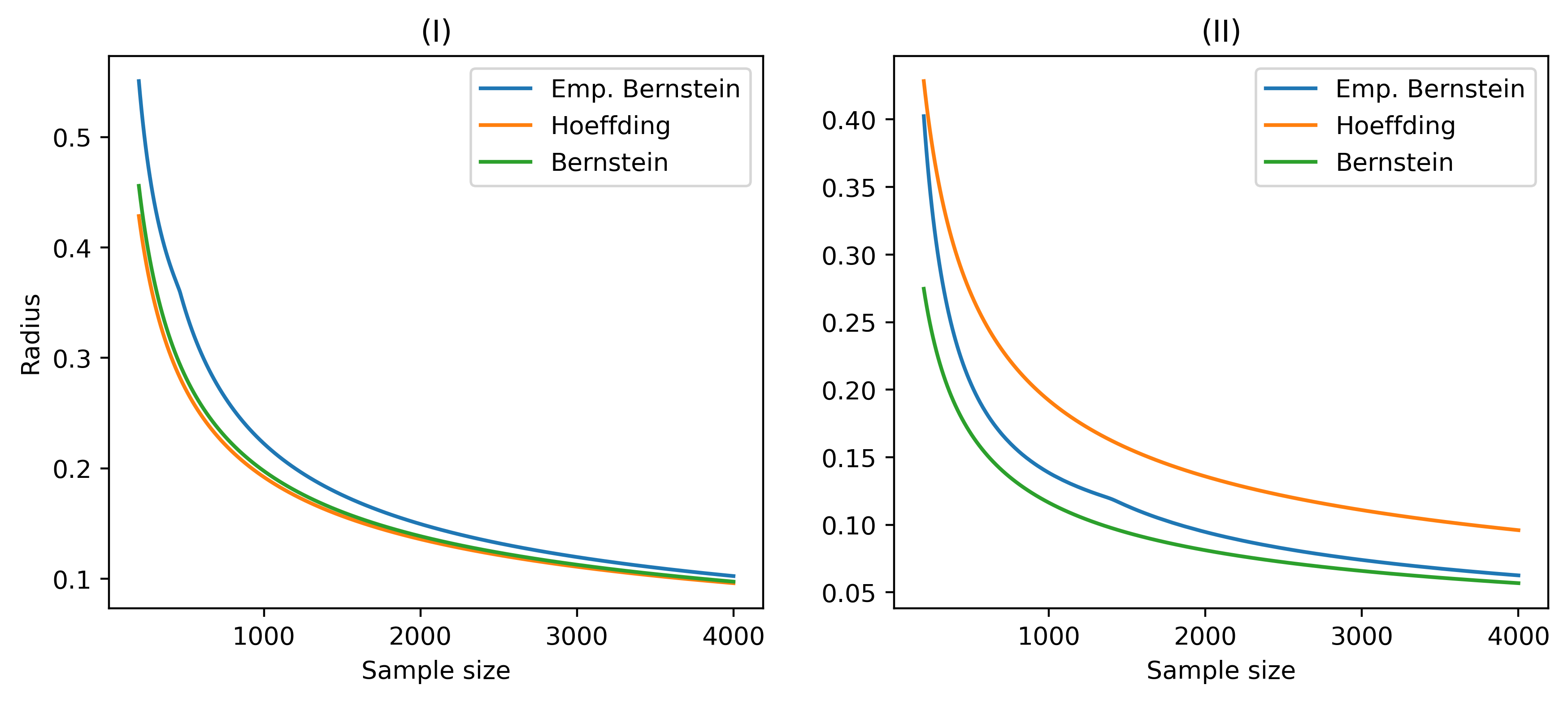
Figure 1: Radius of the confidence sets given by the empirical Bernstein (our proposal) and Hoeffding/Bernstein type (Pinelis,, 1994, Theorem 3.5) bounds, averaged over $100$ repetitions. The oracle Bernstein-type bound is the target to which we compare the other two. The Hoeffding-type bound is slightly better in the left plot (high variance) but much worse in the right plot (low variance). The empirical Bernstein bound is only slightly worse on both plots, with the difference in widths (even after being multiplied by $\sqrt{n}$) vanishing asymptotically, as indicated by Proposition 1.

5 Proof of Theorem 1

A simpler proof of Theorem 1 restricted to separable real Hilbert spaces may be found in Appendix B; the reader may find it helpful as it elucidates the same key ideas without dealing with the extra technical challenges that arise in Banach spaces. We defer the proofs of all the auxiliary lemmas below to Appendix A.

Proof of Theorem 1.

The proof follows a similar high level strategy to Pinelis, (1994, Theorem 3.2), with several additional technical challenges to deal with the estimated variance and the $\psi_{E}$ function defined above.

First, we prove that it suffices to establish the result for random variables that only take a finite number of values in a finite dimensional Banach space. Second, we smoothen the norm in the finite dimensional Banach space so that it is Fréchet differentiable at any arbitrary point. Third, we derive two inequalities that play a central role in the proof. Fourth, we conclude the result by constructing a nonnegative supermartingale, while exploiting the Fréchet differentiability of the smoothened function in the process alongside the previous inequalities.

Step 1: From arbitrary Banach spaces to finite dimensional Banach spaces

Our first goal is to prove that, if (3) is a supermartingale for random variables that take a finite number of values in finite dimensional Banach spaces, then Theorem 1 follows. In order to do so, we approximate the original process by processes that only take a finite number of values. The following lemma extends Pinelis, (1994, Lemma 2.3) to accommodate for a predictable process.

Lemma 1.

Let $(M_{t})_{t\geq 1}$ be a martingale in a separable Banach space $(\mathcal{X},\|\cdot\|)$ and $(\lambda_{t})_{t\geq 1}$ be a predictable real-valued sequence, both relative to filtration $(\mathcal{F}_{t})_{t\geq 0}$. Then, for any $\epsilon>0$, there exist a martingale $(M_{t,\epsilon})_{t\geq 1}$ and a predictable sequence $(\lambda_{t,\epsilon})_{t\geq 1}$ , both relative to a filtration $(\mathcal{F}_{t,\epsilon})_{t\geq 0}$, such that

• $M_{t,\epsilon}$ and $\lambda_{t+1,\epsilon}$ are random variables having only a finite number of values,

• $V_{t,\epsilon}\to V_{t}$ in probability as $\epsilon\downarrow 0$ for any $t\geq 1$,

where $V_{t}=((0,\lambda_{1}),(M_{1},\lambda_{2}),\ldots,(M_{t},\lambda_{t+1}))$ and $V_{t,\epsilon}=((0,\lambda_{1,\epsilon}),(M_{1,\epsilon},\lambda_{2,\epsilon}),\ldots,(M_{t,\epsilon},\lambda_{t+1,\epsilon}))$.

Let $V_{t}$ and $V_{t,\epsilon}$ be defined as in the lemma above, with $M_{i}=X_{i}-\mu$ and $M_{i,\epsilon}=X_{i,\epsilon}-\mu$, and we take $M_{0}:=0$ by default. Lemma 1 implies that $\left\|V_{t,\epsilon}-V_{t}\right\|_{\infty}\stackrel{{\scriptstyle}}{{\to}}0$ in probability as $\epsilon\downarrow 0$. Now note that the function

$$\Pi:(\mathcal{X}\times[0,1))^{t} \longrightarrow\mathbb{R}^{t}$$

$$((m_{0},\lambda_{1}),\ldots,(m_{t},\lambda_{t+1})) \longmapsto\left(\cosh\left(\left\|\sum_{i=1}^{j}\lambda_{i}\frac{m_{i}}{4BD}\right\|\right)\exp\left(-\sum_{i=1}^{j}\frac{\psi_{E}(\lambda_{i})}{(4B)^{2}}\|m_{i}+\mu-\bar{\mu}_{i-1}\|^{2}\right)\right)_{j=1}^{t}$$

is continuous. Note that $m_{0}$ does not appear on the right hand side above. We observe that $(\mathcal{X}\times[0,1/2])^{t}$ is the direct product of separable Banach spaces, and hence a separable Banach space itself. By the continuous mapping theorem on separable Banach spaces (Bosq,, 2000, Theorem 2.3), it follows that $\left\|\Pi(V_{t,\epsilon})-\Pi(V_{t})\right\|_{\infty}\stackrel{{\scriptstyle}}{{\to}}0$ in probability as $\epsilon\downarrow 0$. Furthermore, $\sup_{\epsilon}\left\|\Pi(V_{t,\epsilon})\right\|_{\infty}\leq\cosh(\frac{t}{2D})$, given that

$$\left\|\sum_{i=1}^{t}\lambda_{i}\frac{M_{i}}{4BD}\right\|\leq\sum_{i=1}^{t}\lambda_{i}\frac{1}{2D}\leq\frac{t}{2D}.$$

Lemma 2.

For any $\epsilon>0$, let $(W_{t,\epsilon})_{t\geq 1}$ be a real valued supermartingale. If, for all $t\geq 1$,

1. $(W_{1,\epsilon},\ldots,W_{t,\epsilon})$ converges to $(W_{1},\ldots,W_{t})$ in probability as $\epsilon\downarrow 0$,

2. $\sup_{\epsilon}\left\|(W_{1,\epsilon},\ldots,W_{t,\epsilon})\right\|_{\infty}\leq C_{t}$ for some $C_{t}<\infty$,

then $(W_{t})_{t\geq 1}$ is a supermartingale.

In view of Lemma 2 (taking $(W_{1,\epsilon},\ldots,W_{t,\epsilon})=\Pi(V_{t,\epsilon})$ and $(W_{1},\ldots,W_{t})=\Pi(V_{t})$), the convergence in probability of $\Pi(V_{t,\epsilon})$ to $\Pi(V_{t})$, alongside its boundedness, suffices to preserve the supermartingale property from $\Pi(V_{t,\epsilon})$ to $\Pi(V_{t})$. Note that $\Pi(V_{t})=S_{t}$, and $\Pi(V_{t,\epsilon})$ is a process of the form $S_{t}$ with $V_{t,\epsilon}$ taking a finite number of values in a finite dimensional Banach space.

Step 2: Smoothening the norm of a finite dimensional 2-smooth Banach space

Before we turn to prove the supermartingale condition of such processes, let us note that $(V_{t,\epsilon})_{t\leq n}$ takes only a finite number of values in a separable Banach space, and thus it suffices to work with the finite dimensional Banach subspace spanned by those vectors. It turns out that, in finite dimensional Banach spaces, it is easy to approximate the norm by a smooth function. This will allow us to take derivatives in these ‘smoothed’ spaces, and then generalize the result to the original norm by passing to the limit. We start by presenting Pinelis, (1994, Lemma 2.2), stated below for completeness.

Lemma 3.

Let $(\mathcal{X},\|\cdot\|)$ be $(2,D)$-smooth finite-dimensional Banach space. Define

$$\Upsilon_{\epsilon}(x)=\sqrt{\int_{\mathcal{X}}\|x-\epsilon y\|^{2}\gamma(dy)},$$

where $\gamma$ is a zero-mean Gaussian measure on $\mathcal{X}$ with support $\mathcal{X}$. Then for $\epsilon>0$, $\Upsilon_{\epsilon}$ has the Fréchet derivatives of any order, and the directional derivatives in any direction $v\in\mathcal{X}$ satisfy the inequalities

$$|\Upsilon_{\epsilon}^{\prime}(x)(v)|\leq\|v\|,\quad(\Upsilon^{2}_{\epsilon})^{\prime\prime}(x)(v,v)\leq 2D^{2}\|v\|^{2}$$ (5)

for all $x\in\mathcal{X}$. Besides, for each $x\in\mathcal{X}$, $\Upsilon_{\epsilon}(x)\to\|x\|$ as $\epsilon\downarrow 0$.

Note that the existence of the Gaussian measure $\gamma$ in Lemma 3 is evident since the Banach space is finite dimensional. Furthermore, the variance of such a Gaussian measure is irrelevant (as long as its support is the whole space $\mathcal{X}$); intuitively, the role of the parameter $\epsilon$ is precisely to make this variance go to zero as $\epsilon\downarrow 0$.

While the norm of a Banach space may not be Fréchet differentiable at any arbitrary point, its Gateaux derivative in the direction of the point always exists. To see this, take any $x\in B$, and note that $\|x+tx\|=(1+t)\|x\|$ for $t\geq-1$. As a function of $t$, $(1+t)\|x\|$ is clearly $C^{\infty}$, and its derivative at $0$ takes the value $\|x\|$. This behaviour still holds for $\Upsilon_{\epsilon}$, as elucidated in the following lemma.

Lemma 4.

$\lim_{\epsilon\downarrow 0}\Upsilon_{\epsilon}^{\prime}(x)(x)=\|x\|$.

By linearity, Lemma 4 implies that $\lim_{\epsilon\downarrow 0}\Upsilon_{\epsilon}^{\prime}(x)(\gamma x)=\gamma\|x\|$ for all nonnegative $\gamma$. Lastly, we show that $\Upsilon_{\epsilon}$ can be upper bounded in a closed interval for a range of $\epsilon$. This will later allow us to use the dominated convergence theorem.

Lemma 5.

For a $(2,D)$-smooth Banach space, it holds that

$$\Upsilon_{\epsilon}\left(x+\beta y\right)\leq\sqrt{2c(x,y)+2D^{2}C},\quad\forall(x,y)\in\mathcal{X}^{2},\quad\forall(\beta,\epsilon)\in[0,1]^{2},$$

where $c(x,y)=\max(\|x\|,\|x+y\|)$, and $C=\int_{X}\|y\|^{2}\gamma(dy)$.

Step 3: Deriving two central deterministic inequalities

As we shall see in the next step, understanding the interplay between several terms of a Taylor expansion is of crucial importance to conclude the result. In order to do so, we require the two deterministic inequalities presented in this step. We start by presenting a sharp inequality concerning the $\psi_{E}$ function.

Lemma 6.

For all $\lambda\in(0,1/2]$, $x\in(0,1/2]$, and $D\in[1,\infty)$,

$$\frac{\left(\lambda x+\psi_{E}(\lambda)x^{2}\right)^{2}}{\left(\frac{\lambda x}{D}-\psi_{E}(\lambda)x^{2}\right)^{2}}\left(e^{\frac{\lambda x}{D}-\psi_{E}(\lambda)x^{2}}-\left(\frac{\lambda x}{D}-\psi_{E}(\lambda)x^{2}\right)-1\right)\leq\psi_{E}(\lambda)x^{2}.$$

In stark contrast to previously used deterministic inequalities in related contributions (see e.g., Fan et al., (2015, Proposition 4.1)) that may be proven based on the $2$nd degree Taylor coefficient, the proof of Lemma 6 requires to study up to the $7$th degree Taylor coefficient. Lastly, the following lemma establishes an elemental yet powerful inequality concerning hyperbolic functions.

Lemma 7.

For all $x,y\in\mathbb{R}$,

$$\cosh(y+x)-x\sinh(y+x)-\cosh(y)\leq 0.$$

Step 4: Concluding the proof with a supermartingale construction

Throughout, we assume that $(X_{1},\ldots,X_{n})$ only takes a finite number of values. The process $S_{t}$ is nonnegative given that both the $\exp$ and $\cosh$ functions are nonnegative, so all we ought to prove is that such a process is a supermartingale, i.e.,

$$\mathbb{E}_{t-1}\left[S_{t}\right]\leq S_{t-1}.$$

Based on Lemma 3,

$$S_{t}=\lim_{\epsilon\downarrow 0}\left[\cosh\left(\Upsilon_{\epsilon}\left(\sum_{i=1}^{t}\lambda_{i}\frac{X_{i}-\mu}{4BD}\right)\right)\exp\left(-\sum_{i=1}^{t}\frac{\psi_{E}(\lambda_{i})}{(4B)^{2}}\|X_{i}-\bar{\mu}_{i-1}\|^{2}\right)\right],$$

and so

$$\mathbb{E}_{t-1}\left[S_{t}\right]=\mathbb{E}_{t-1}\left[\lim_{\epsilon\downarrow 0}\left[\cosh\left(\Upsilon_{\epsilon}\left(\sum_{i=1}^{t}\lambda_{i}\frac{X_{i}-\mu}{4BD}\right)\right)\exp\left(-\sum_{i=1}^{t}\frac{\psi_{E}(\lambda_{i})}{(4B)^{2}}\|X_{i}-\bar{\mu}_{i-1}\|^{2}\right)\right]\right].$$

Let us denote

$$Y_{i}=\frac{X_{i}-\mu}{4B},\quad\delta_{t}=\frac{\bar{\mu}_{t}-\mu}{4B},\quad Z_{i}=Y_{i}-\delta_{i-1},$$

as well as

$$M_{t}=\sum_{i=1}^{t}\lambda_{i}\frac{X_{i}-\mu}{4BD},\quad R_{t}=\exp\left(-\sum_{i=1}^{t}\frac{\psi_{E}(\lambda_{i})}{(4B)^{2}}\|X_{i}-\bar{\mu}_{i-1}\|^{2}\right),\quad A_{t}=M_{t-1}+\frac{\lambda_{t}}{D}\delta_{t-1}.$$

We define

$$\varphi_{t,\epsilon}(\beta) =R_{t-1}\cosh\Upsilon_{\epsilon}\left(M_{t-1}+\frac{\lambda_{t}}{D}\delta_{t-1}+\beta\frac{\lambda_{t}}{D}\left(\frac{X_{t}-\mu}{4B}-\delta_{t-1}\right)\right)\exp\left(-\beta\frac{\psi_{E}(\lambda_{t})}{(4B)^{2}}\|X_{t}-\bar{\mu}_{t-1}\|^{2}\right)$$

$$=R_{t-1}\Upsilon_{\epsilon}\left(M_{t-1}+\frac{\lambda_{t}}{D}\delta_{t-1}+\beta\frac{\lambda_{t}}{D}\left(Y_{t}-\delta_{t-1}\right)\right)\exp\left(-\beta\psi_{E}(\lambda_{t})\|Y_{t}-\delta_{t-1}\|^{2}\right)$$

$$=R_{t-1}\cosh\Upsilon_{\epsilon}\left(A_{t}+\beta\frac{\lambda_{t}}{D}Z_{t}\right)\exp\left(-\beta\psi_{E}(\lambda_{t})\|Z_{t}\|^{2}\right).$$

We exploit its Taylor expansion

$$\varphi_{t,\epsilon}(1)=\varphi_{t,\epsilon}(0)+\varphi_{t,\epsilon}^{\prime}(0)+\int_{0}^{1}(1-\beta)\varphi_{t,\epsilon}^{\prime\prime}(\beta)d\beta.$$

Now we observe that

$$\mathbb{E}_{t-1}\left[S_{t}\right] =\mathbb{E}_{t-1}\left[\lim_{\epsilon\downarrow 0}\varphi_{t,\epsilon}(1)\right]$$

$$\stackrel{{\scriptstyle(i)}}{{=}}\lim_{\epsilon\downarrow 0}\mathbb{E}_{t-1}\left[\varphi_{t,\epsilon}(1)\right]$$

$$=\lim_{\epsilon\downarrow 0}\mathbb{E}_{t-1}\left[\varphi_{t,\epsilon}(0)+\varphi_{t,\epsilon}^{\prime}(0)+\int_{0}^{1}(1-\beta)\varphi_{t,\epsilon}^{\prime\prime}(\beta)d\beta\right]$$

$$\leq\limsup_{\epsilon\downarrow 0}\mathbb{E}_{t-1}\left[\varphi_{t,\epsilon}(0)\right]+\limsup_{\epsilon\downarrow 0}\mathbb{E}_{t-1}\left[\varphi_{t,\epsilon}^{\prime}(0)\right]+\limsup_{\epsilon\downarrow 0}\mathbb{E}_{t-1}\left[\int_{0}^{1}(1-\beta)\varphi_{t,\epsilon}^{\prime\prime}(\beta)d\beta\right].$$ (6)

where (i) is obtained given that the limit transition preserves linear combinations. Now we analyze the three terms. First, note that $\varphi_{t,\epsilon}(0)=\mathbb{E}_{t-1}\left[\varphi_{t,\epsilon}(0)\right]=R_{t-1}\cosh\Upsilon_{\epsilon}\left(A_{t}\right)$. By Lemma 3,

$$\limsup_{\epsilon\downarrow 0}\varphi_{t,\epsilon}(0)=\limsup_{\epsilon\downarrow 0}\left[R_{t-1}\cosh\Upsilon_{\epsilon}\left(A_{t}\right)\right]=R_{t-1}\cosh\left(\lim_{\epsilon\downarrow 0}\Upsilon_{\epsilon}\left(A_{t}\right)\right)=R_{t-1}\cosh\left\|A_{t}\right\|.$$ (7)

Second,

$$\frac{\varphi_{t,\epsilon}^{\prime}(\beta)}{R_{t-1}} =\frac{d}{d\beta}\left(\cosh\Upsilon_{\epsilon}\left(A_{t}+\beta\frac{\lambda_{t}}{D}Z_{t}\right)\exp\left(-\beta\psi_{E}(\lambda_{t})\|Z_{t}\|^{2}\right)\right)$$

$$=\exp\left(-\beta\psi_{E}(\lambda_{t})\|Z_{t}\|^{2}\right)\sinh\Upsilon_{\epsilon}\left(A_{t}+\beta\frac{\lambda_{t}}{D}Z_{t}\right)\Upsilon_{\epsilon}^{\prime}\left(A_{t}+\beta\frac{\lambda_{t}}{D}Z_{t}\right)\left(\frac{\lambda_{t}}{D}Z_{t}\right)$$

$$\quad-\psi_{E}(\lambda_{t})\|Z_{t}\|^{2}\cosh\Upsilon_{\epsilon}\left(A_{t}+\beta\frac{\lambda_{t}}{D}Z_{t}\right)\exp\left(-\beta\psi_{E}(\lambda_{t})\|Z_{t}\|^{2}\right).$$

Hence

$$\frac{\varphi^{\prime}_{t,\epsilon}(0)}{R_{t-1}} =\sinh\Upsilon_{\epsilon}\left(A_{t}\right)\Upsilon_{\epsilon}^{\prime}\left(A_{t}\right)\left(\frac{\lambda_{t}}{D}Z_{t}\right)-\psi_{E}(\lambda_{t})\|Z_{t}\|^{2}\cosh\Upsilon_{\epsilon}\left(A_{t}\right),$$

and so

$$\mathbb{E}\left[\frac{\varphi^{\prime}_{t,\epsilon}(0)}{R_{t-1}}\right] =\mathbb{E}\left[\sinh\Upsilon_{\epsilon}\left(A_{t}\right)\Upsilon_{\epsilon}^{\prime}\left(A_{t}\right)\left(\frac{\lambda_{t}}{D}Z_{t}\right)\right]-\mathbb{E}\left[\psi_{E}(\lambda_{t})\|Z_{t}\|^{2}\cosh\Upsilon_{\epsilon}\left(A_{t}\right)\right]$$

$$=\sinh\Upsilon_{\epsilon}\left(A_{t}\right)\Upsilon_{\epsilon}^{\prime}\left(A_{t}\right)\left(\mathbb{E}\left[\frac{\lambda_{t}}{D}Z_{t}\right]\right)-\mathbb{E}\left[\psi_{E}(\lambda_{t})\|Z_{t}\|^{2}\cosh\Upsilon_{\epsilon}\left(A_{t}\right)\right]$$

$$=\sinh\Upsilon_{\epsilon}\left(A_{t}\right)\Upsilon_{\epsilon}^{\prime}\left(A_{t}\right)\left(\mathbb{E}\left[\frac{\lambda_{t}}{D}(Y_{t}-\delta_{t-1})\right]\right)-\mathbb{E}\left[\psi_{E}(\lambda_{t})\|Z_{t}\|^{2}\cosh\Upsilon_{\epsilon}\left(A_{t}\right)\right]$$

$$\stackrel{{\scriptstyle(i)}}{{=}}-\sinh\Upsilon_{\epsilon}\left(A_{t}\right)\Upsilon_{\epsilon}^{\prime}\left(A_{t}\right)\left(\frac{\lambda_{t}}{D}\delta_{t-1}\right)-\mathbb{E}\left[\psi_{E}(\lambda_{t})\|Z_{t}\|^{2}\cosh\Upsilon_{\epsilon}\left(A_{t}\right)\right],$$

where (i) is obtained due to $\mathbb{E}_{t-1}[Y_{t}]=0$. Note that $\delta_{t-1}$ is simply $M_{t-1}$ rescaled by a positive factor, and so they are both aligned to $A_{t}=M_{t-1}+\frac{\lambda_{t}}{D}\delta_{t-1}$. Based on Lemma 4, this implies that

$$\lim_{\epsilon\downarrow 0}\left[\sinh\Upsilon_{\epsilon}\left(A_{t}\right)\Upsilon_{\epsilon}^{\prime}\left(A_{t}\right)\left(\frac{\lambda_{t}}{D}\delta_{t-1}\right)\right] =\left[\lim_{\epsilon\downarrow 0}\sinh\Upsilon_{\epsilon}\left(A_{t}\right)\right]\left[\lim_{\epsilon\downarrow 0}\Upsilon_{\epsilon}^{\prime}\left(A_{t}\right)\left(\frac{\lambda_{t}}{D}\delta_{t-1}\right)\right]$$

$$=\left\|\frac{\lambda_{t}}{D}\delta_{t-1}\right\|\sinh(\|A_{t}\|).$$

Thus,

$$\limsup_{\epsilon\downarrow 0}\mathbb{E}\left[\frac{\varphi^{\prime}_{t,\epsilon}(0)}{R_{t-1}}\right] =-\frac{\lambda_{t}}{D}\left\|\delta_{t-1}\right\|\sinh(\|A_{t}\|)-\lim_{\epsilon\downarrow 0}\mathbb{E}\left[\psi_{E}(\lambda_{t})\|Z_{t}\|^{2}\cosh\Upsilon_{\epsilon}\left(A_{t}\right)\right]$$

$$\stackrel{{\scriptstyle(i)}}{{=}}-\frac{\lambda_{t}}{D}\left\|\delta_{t-1}\right\|\sinh(\|A_{t}\|)-\mathbb{E}\left[\lim_{\epsilon\downarrow 0}\left[\psi_{E}(\lambda_{t})\|Z_{t}\|^{2}\cosh\Upsilon_{\epsilon}\left(A_{t}\right)\right]\right]$$

$$=-\frac{\lambda_{t}}{D}\left\|\delta_{t-1}\right\|\sinh(\|A_{t}\|)-\mathbb{E}\left[\psi_{E}(\lambda_{t})\|Z_{t}\|^{2}\cosh\|A_{t}\|\right],$$ (8)

where (i) is obtained given that the limit transition preserves linear combinations.

Third,

$$\frac{\varphi_{t,\epsilon}^{\prime\prime}(\beta)}{R_{t-1}}\exp\left(\beta\psi_{E}(\lambda_{t})\|Z_{t}\|^{2}\right) =\cosh\Upsilon_{\epsilon}\left(A_{t}+\beta\frac{\lambda_{t}}{D}Z_{t}\right)\left[\Upsilon_{\epsilon}^{\prime}\left(A_{t}+\beta\frac{\lambda_{t}}{D}Z_{t}\right)\left(\frac{\lambda_{t}}{D}Z_{t}\right)\right]^{2}$$

$$\quad+\sinh\Upsilon_{\epsilon}\left(A_{t}+\beta\frac{\lambda_{t}}{D}Z_{t}\right)\Upsilon_{\epsilon}^{\prime\prime}\left(A_{t}+\beta\frac{\lambda_{t}}{D}Z_{t}\right)\left(\frac{\lambda_{t}}{D}Z_{t}\right)$$

$$\quad-2\psi_{E}(\lambda_{t})\|Z_{t}\|^{2}\sinh\Upsilon_{\epsilon}\left(A_{t}+\beta\frac{\lambda_{t}}{D}Z_{t}\right)\Upsilon_{\epsilon}^{\prime}\left(A_{t}+\beta\frac{\lambda_{t}}{D}Z_{t}\right)\left(\frac{\lambda_{t}}{D}Z_{t}\right)$$

$$\quad+\left(\psi_{E}(\lambda_{t})\|Z_{t}\|^{2}\right)^{2}\cosh\Upsilon_{\epsilon}\left(A_{t}+\beta\frac{\lambda_{t}}{D}Z_{t}\right).$$

We note that $\sinh u\leq u\cosh u$ if, and only if, $u\geq 0$. This implies that, when $u^{\prime\prime}u>0$, one has $(\cosh u)^{\prime\prime}=u^{\prime 2}\cosh u+u^{\prime\prime}\sinh u\leq(u^{\prime 2}+u^{\prime\prime}u)\cosh u=\frac{1}{2}(u^{2})^{\prime\prime}\cosh u$ . If $u^{\prime\prime}u\leq 0$, then $(\cosh u)^{\prime\prime}\leq u^{\prime 2}\cosh u$. Thus $(\cosh u)^{\prime\prime}\leq\max(\frac{1}{2}(u^{2})^{\prime\prime},u^{\prime 2})\cosh u$. Taking $u=\Upsilon_{\epsilon}\left(A_{t}+\beta\lambda_{t}Z_{t}/D\right)$, and in view of Lemma 3,

$$\max(\frac{1}{2}(u^{2})^{\prime\prime},u^{\prime 2})\leq D^{2}\left\|\frac{\lambda_{t}}{D}Z_{t}\right\|^{2}=\left\|\lambda_{t}Z_{t}\right\|^{2}.$$

Consequently, $(\cosh u)^{\prime\prime}$ is equal to

$$\cosh\Upsilon_{\epsilon}\left(A_{t}+\beta\frac{\lambda_{t}}{D}Z_{t}\right)\left[\Upsilon_{\epsilon}^{\prime}\left(A_{t}+\beta\frac{\lambda_{t}}{D}Z_{t}\right)\left(\frac{\lambda_{t}}{D}Z_{t}\right)\right]^{2}+\sinh\Upsilon_{\epsilon}\left(A_{t}+\beta\frac{\lambda_{t}}{D}Z_{t}\right)\Upsilon_{\epsilon}^{\prime\prime}\left(A_{t}+\beta\frac{\lambda_{t}}{D}Z_{t}\right)\left(\frac{\lambda_{t}}{D}Z_{t}\right)$$

and is upper bounded by $\cosh\Upsilon_{\epsilon}\left(A_{t}+\beta\frac{\lambda_{t}}{D}Z_{t}\right)\left\|\lambda_{t}Z_{t}\right\|^{2}$. Furthermore,

$$\left|-2\psi_{E}(\lambda_{t})\|Z_{t}\|^{2}\sinh\Upsilon_{\epsilon}\left(A_{t}+\beta\frac{\lambda_{t}}{D}Z_{t}\right)\Upsilon_{\epsilon}^{\prime}\left(A_{t}+\beta\frac{\lambda_{t}}{D}Z_{t}\right)\left(\frac{\lambda_{t}}{D}Z_{t}\right)\right|$$

is upper bounded by $2\psi_{E}(\lambda_{t})\|Z_{t}\|^{2}\cosh\Upsilon_{\epsilon}\left(A_{t}+\beta\frac{\lambda_{t}}{D}Z_{t}\right)\left\|\lambda_{t}Z_{t}\right\|$ given that $\sinh u\leq\cosh u$, Lemma 3, and $D\geq 1$. Thus,

$$\frac{\varphi_{t,\epsilon}^{\prime\prime}(\beta)}{R_{t-1}}\exp\left(\beta\psi_{E}(\lambda_{t})\|Z_{t}\|^{2}\right) \leq\cosh\Upsilon_{\epsilon}\left(A_{t}+\beta\frac{\lambda_{t}}{D}Z_{t}\right)\left\|\lambda_{t}Z_{t}\right\|^{2}$$

$$\quad+2\psi_{E}(\lambda_{t})\|Z_{t}\|^{2}\cosh\Upsilon_{\epsilon}\left(A_{t}+\beta\frac{\lambda_{t}}{D}Z_{t}\right)\left\|\lambda_{t}Z_{t}\right\|$$

$$\quad+\left(\psi_{E}(\lambda_{t})\|Z_{t}\|^{2}\right)^{2}\cosh\Upsilon_{\epsilon}\left(A_{t}+\beta\frac{\lambda_{t}}{D}Z_{t}\right)$$

$$=\left(\psi_{E}(\lambda_{t})\|Z_{t}\|^{2}+\|\lambda_{t}Z_{t}\|\right)^{2}\cosh\Upsilon_{\epsilon}\left(A_{t}+\beta\frac{\lambda_{t}}{D}Z_{t}\right).$$

We note that

$$\limsup_{\epsilon\downarrow 0}\mathbb{E}_{t-1}\left[\int_{0}^{1}(1-\beta)\varphi_{t,\epsilon}^{\prime\prime}(\beta)d\beta\right]\leq\mathbb{E}_{t-1}\left[\limsup_{\epsilon\downarrow 0}\int_{0}^{1}(1-\beta)\varphi_{t,\epsilon}^{\prime\prime}(\beta)d\beta\right],$$

and denoting $H_{t}=R_{t-1}\left(\psi_{E}(\lambda_{t})\|Z_{t}\|^{2}+\|\lambda_{t}Z_{t}\|\right)^{2}$, we observe that

$$\limsup_{\epsilon\downarrow 0}\int_{0}^{1}(1-\beta)\varphi_{t,\epsilon}^{\prime\prime}(\beta)d\beta\leq H_{t}\limsup_{\epsilon\downarrow 0}\int_{0}^{1}(1-\beta)\cosh\Upsilon_{\epsilon}\left(A_{t}+\beta\frac{\lambda_{t}}{D}Z_{t}\right)\exp\left(-\beta\psi_{E}(\lambda_{t})\|Z_{t}\|^{2}\right)d\beta.$$ (9)

In view of Lemma 5, $(1-\beta)\cosh\Upsilon_{\epsilon}\left(A_{t}+\beta\frac{\lambda_{t}}{D}Z_{t}\right)\exp\left(-\beta\psi_{E}(\lambda_{t})\|Z_{t}\|^{2}\right)$ is dominated for all $\beta\in[0,1]$ and $\epsilon\in[0,1]$. The dominated convergence theorem implies that the $\limsup$ on the right hand side of (9) is actually a $\lim$ and is equal to

$$H_{t}\int_{0}^{1}(1-\beta)\left[\lim_{\epsilon\downarrow 0}\cosh\Upsilon_{\epsilon}\left(A_{t}+\beta\frac{\lambda_{t}}{D}Z_{t}\right)\right]\exp\left(-\beta\psi_{E}(\lambda_{t})\|Z_{t}\|^{2}\right)d\beta$$

$$= H_{t}\int_{0}^{1}(1-\beta)\cosh\left\|A_{t}+\beta\frac{\lambda_{t}}{D}Z_{t}\right\|\exp\left(-\beta\psi_{E}(\lambda_{t})\|Z_{t}\|^{2}\right)d\beta$$

$$\leq H_{t}\int_{0}^{1}(1-\beta)\cosh\left\|A_{t}\right\|\exp\left(\beta\left\|\frac{\lambda_{t}}{D}Z_{t}\right\|-\beta\psi_{E}(\lambda_{t})\|Z_{t}\|^{2}\right)d\beta$$

$$\stackrel{{\scriptstyle(i)}}{{=}} H_{t}\cosh\left\|A_{t}\right\|\frac{\exp\left(\left\|\frac{\lambda_{t}}{D}Z_{t}\right\|-\psi_{E}(\lambda_{t})\|Z_{t}\|^{2}\right)-\left(\left\|\frac{\lambda_{t}}{D}Z_{t}\right\|-\psi_{E}(\lambda_{t})\|Z_{t}\|^{2}\right)-1}{\left(\left\|\frac{\lambda_{t}}{D}Z_{t}\right\|-\psi_{E}(\lambda_{t})\|Z_{t}\|^{2}\right)^{2}}$$

$$= R_{t-1}\cosh\left\|A_{t}\right\|\left(\psi_{E}(\lambda_{t})\|Z_{t}\|^{2}+\left\|\lambda_{t}Z_{t}\right\|\right)^{2}\times$$

$$\quad\times\frac{\exp\left(\left\|\frac{\lambda_{t}}{D}Z_{t}\right\|-\psi_{E}(\lambda_{t})\|Z_{t}\|^{2}\right)-\left(\left\|\frac{\lambda_{t}}{D}Z_{t}\right\|-\psi_{E}(\lambda_{t})\|Z_{t}\|^{2}\right)-1}{\left(\left\|\frac{\lambda_{t}}{D}Z_{t}\right\|-\psi_{E}(\lambda_{t})\|Z_{t}\|^{2}\right)^{2}}$$

$$\stackrel{{\scriptstyle(ii)}}{{\leq}}R_{t-1}\cosh\left\|A_{t}\right\|\psi_{E}(\lambda)\|Z_{t}\|^{2},$$

where equality (i) is obtained from $\int_{0}^{1}(1-\beta)e^{a\beta}d\beta=\frac{e^{a}-a-1}{a^{2}}$, and inequality (ii) follows from Lemma 6. Thus,

$$\limsup_{\epsilon\downarrow 0}\mathbb{E}_{t-1}\left[\int_{0}^{1}(1-\beta)\varphi_{t,\epsilon}^{\prime\prime}(\beta)d\beta\right]\leq\mathbb{E}_{t-1}\left[R_{t-1}\cosh\left\|A_{t}\right\|\psi_{E}(\lambda)\|Z_{t}\|^{2}\right].$$ (10)

We observe that (6) is upper bounded by the sum of (7), (8), and (10), which add up to

$$R_{t-1}\left\{\cosh\left\|A_{t}\right\|-\frac{\lambda_{t}}{D}\left\|\delta_{t-1}\right\|\sinh(\|A_{t}\|)\right\}.$$

Given that $\delta_{t-1}$ is simply $M_{t-1}$ re-scaled by a positive factor, it follows that $A_{t}=\left\|M_{t-1}+\frac{\lambda_{t}}{D}\delta_{t-1}\right\|=\left\|M_{t-1}\right\|+\left\|\frac{\lambda_{t}}{D}\delta_{t-1}\right\|$. Thus,

$$-\left\|\frac{\lambda_{t}}{D}\delta_{t-1}\right\|\sinh\left\|A_{t}\right\| =-\left\|\lambda_{t}\delta_{t-1}\right\|\sinh\left\|M_{t-1}+\frac{\lambda_{t}}{D}\delta_{t-1}\right\|$$

$$=-\left\|\frac{\lambda_{t}}{D}\delta_{t-1}\right\|\sinh\left(\left\|M_{t-1}\right\|+\left\|\frac{\lambda_{t}}{D}\delta_{t-1}\right\|\right)$$

$$\stackrel{{\scriptstyle(i)}}{{\leq}}\cosh\left\|M_{t-1}\right\|-\cosh\left(\left\|M_{t-1}\right\|+\left\|\frac{\lambda_{t}}{D}\delta_{t-1}\right\|\right)$$

$$\stackrel{{\scriptstyle}}{{=}}\cosh\left\|M_{t-1}\right\|-\cosh\left\|M_{t-1}+\frac{\lambda_{t}}{D}\delta_{t-1}\right\|$$

$$\stackrel{{\scriptstyle}}{{=}}\cosh\left\|M_{t-1}\right\|-\cosh\left\|A_{t}\right\|,$$

where (i) is obtained in view of Lemma 7. We conclude the proof by noting that

$$\mathbb{E}_{t-1}\left[S_{t}\right] \leq R_{t-1}\left\{\cosh\left\|A_{t}\right\|-\frac{\lambda_{t}}{D}\left\|\delta_{t-1}\right\|\sinh(\|A_{t}\|)\right\}$$

$$\leq R_{t-1}\left\{\cosh\left\|A_{t}\right\|+\cosh\left\|M_{t-1}\right\|-\cosh\left\|A_{t}\right\|\right\}$$

$$=R_{t-1}\cosh\left\|M_{t-1}\right\|$$

$$=S_{t-1}.$$

∎

6 Summary

Current concentration inequalities for bounded vector-valued random variables encompass extensions of the Hoeffding and Bernstein inequalities. Although Bernstein’s inequality is generally tighter than Hoeffding’s, it requires to know an upper bound on the variance of the random variables (which is generally unknown). The primary contribution of this current work is to provide a vector-valued empirical Bernstein concentration bound, which replaces the true variance by its empirical estimator. The subsequent confidence sets are typically tighter than those provided by the vector-valued Hoeffding inequality, and are actionable in practice. The proposed empirical Bernstein holds in 2-smooth separable Banach spaces, which include finite dimensional Euclidean spaces and separable Hilbert spaces. The bound extends the empirical Bernstein concentration inequality from Waudby-Smith and Ramdas, (2024) to this more general setting, and its proof combines novel deterministic inequalities with some of the theoretical tools presented in Pinelis, (1994) to derive a nonnegative supermartingale construction. This nonnegative supermartingale, in conjunction with Ville’s inequality, gives way to both fixed sample size confidence sets (batch setting) and anytime-valid confidence sequences (sequential setting). The empirical performance of the proposed empirical Bernstein for different multivariate bounded distributions is also exhibited.

Acknowledgements

The authors thank Ben Chugg and Martin Larsson for insightful conversations. DMT gratefully acknowledges that the project that gave rise to these results received the support of a fellowship from ‘la Caixa’ Foundation (ID 100010434). The fellowship code is LCF/BQ/EU22/11930075. AR was funded by NSF grant DMS-2310718.

Appendix A Proofs of auxiliary lemmas used in Theorem 1

A.1 Proof of Lemma 1

Take $\mathcal{X}\times\mathbb{R}$ to be the direct product of Banach spaces with norm $\|(m,\gamma)\|=\max(\|m\|,|\gamma|)$ for all $(m,\gamma)\in\mathcal{X}\times\mathbb{R}$. Note that both $\mathcal{X}$ and $\mathbb{R}$ are separable Banach spaces, and thus so is $\mathcal{X}\times\mathbb{R}$. Let $(\left\{B_{k,\epsilon}:k=1,\ldots,k(j,\epsilon)\right\})_{j=0}^{\infty}$ be an increasing sequence of sets of balls in $\mathcal{X}\times\mathbb{R}$ of radius $\epsilon$ such that $k(0,\epsilon)<k(1,\epsilon)<k(2,\epsilon)<\ldots$ and

$$\mathbb{P}\left(\bigcap_{i=1}^{j}\bigcup_{k=1}^{k(j,\epsilon)}\left\{(M_{i},\lambda_{i+1})\in B_{k,\epsilon}\right\}\right)\geq 1-\epsilon,\quad j=1,2,\ldots.$$ (11)

The existence of such a sequence of sets is guaranteed by the tightness of any probability measure on a separable Banach space. Consider the approximations $M_{t,\epsilon}=\mathbb{E}[M_{t}|\mathcal{F}_{t,\epsilon}]$ and $\lambda_{t+1,\epsilon}=\mathbb{E}[\lambda_{t+1}|\mathcal{F}_{t,\epsilon}]$, where $\mathcal{F}_{t,\epsilon}$ is the $\sigma$-field generated by all the events of the form

$$\{(M_{i},\lambda_{i+1})\in B_{k,\epsilon}\},\quad i=0,1,\ldots,j,\quad k=1\ldots,k(j,\epsilon).$$

Note that $M_{t,\epsilon}$ is a martingale with respect to $(\mathcal{F}_{t,\epsilon})_{t\geq 1}$, given that $\mathbb{E}[M_{t,\epsilon}|\mathcal{F}_{t-1,\epsilon}]=\mathbb{E}[\mathbb{E}[M_{t}|\mathcal{F}_{t,\epsilon}]|\mathcal{F}_{t-1,\epsilon}]=\mathbb{E}[M_{t}|\mathcal{F}_{t-1,\epsilon}]=\mathbb{E}[\mathbb{E}[M_{t}|\mathcal{F}_{t-1}]|\mathcal{F}_{t-1,\epsilon}]=\mathbb{E}[M_{t-1}|\mathcal{F}_{t-1,\epsilon}]=M_{t-1,\epsilon}$. Furthermore, $(M_{t,\epsilon},\lambda_{t,\epsilon})$ takes only a finite number of values because the filtration $\mathcal{F}_{t,\epsilon}$ is finite. Lastly,

$$\left\|(M_{i,\epsilon},\lambda_{i+1,\epsilon})-(M_{i},\lambda_{i+1})\right\|\leq 2\epsilon,\quad\forall(M_{i},\lambda_{i+1})\in\bigcup_{k=1}^{k(t,\epsilon)}B_{k,\epsilon},$$

and so

$$\left\|(M_{i,\epsilon},\lambda_{i+1,\epsilon})-(M_{i},\lambda_{i+1})\right\|\leq 2\epsilon$$

simultaneously for all $i\leq t$ with probability at least $1-\epsilon$. Given that $\epsilon$ is arbitrary, the convergence of $V_{t,\epsilon}$ to $V_{t}$ in probability follows.

A.2 Proof of Lemma 2

Let us start by presenting an additional lemma, proved in a later subsection.

Lemma 8.

Let $(W_{t})_{t\geq 1}$ be a real, integrable random process. The statements

1. $\mathbb{E}\left[W_{t}|\sigma\left(W_{1},\ldots,W_{t-1}\right)\right]\leq 0$,

2. $\mathbb{E}\left[W_{t}f(W_{1},\ldots,W_{t-1})\right]\leq 0$ for all nonnegative bounded measurable functions $f$,

3. $\mathbb{E}\left[W_{t}f(W_{1},\ldots,W_{t-1})\right]\leq 0$ for all nonnegative bounded continuous functions $f$,

are equivalent.

Based on Lemma 8, it suffices to check that $\mathbb{E}\left[\left(W_{t}-W_{t-1}\right)f\left(W_{1},\ldots,W_{t-1}\right)\right]\leq 0$ for all nonnegative bounded continuous functions $f$.

Let $f$ be an arbitrary nonnegative bounded continuous function, and let $C_{f}>0$ such that $\|f\|_{\infty}\leq C_{f}$. Denote $Z_{t}=\left(W_{t}-W_{t-1}\right)f\left(W_{1},\ldots,W_{t-1}\right)$ and $Z_{t,\epsilon}=\left(W_{t,\epsilon}-W_{t-1,\epsilon}\right)f\left(W_{1,\epsilon},\ldots,W_{t-1,\epsilon}\right)$. Note that $\mathbb{E}\left[Z_{t,\epsilon}\right]\leq 0$ given that $(W_{t,\epsilon})_{t\geq 1}$ is a supermartingale. Further, $\|Z_{t,\epsilon}\|_{\infty}\leq C:=(C_{t}+C_{t-1})C_{f}$. For $\delta>0$, it follows that

$$\mathbb{E}\left[Z_{t}\right] =\mathbb{E}\left[Z_{t}\mathds{1}(Z_{t}-Z_{t,\epsilon}<\delta)\right]+\mathbb{E}\left[Z_{t}\mathds{1}(Z_{t}-Z_{t,\epsilon}\geq\delta)\right]$$

$$\leq\mathbb{E}\left[(Z_{t,\epsilon}+\delta)\mathds{1}(Z_{t}-Z_{t,\epsilon}<\delta)\right]+\mathbb{E}\left[|Z_{t}|\mathds{1}(Z_{t}-Z_{t,\epsilon}\geq\delta)\right]$$

$$=\mathbb{E}\left[Z_{t,\epsilon}+\delta\right]-\mathbb{E}\left[(Z_{t,\epsilon}+\delta)\mathds{1}(Z_{t}-Z_{t,\epsilon}\geq\delta)\right]+\mathbb{E}\left[|Z_{t}|\mathds{1}(Z_{t}-Z_{t,\epsilon}\geq\delta)\right]$$

$$\leq\delta-(-C+\delta)\mathbb{E}\left[\mathds{1}(Z_{t}-Z_{t,\epsilon}\geq\delta)\right]+\mathbb{E}\left[|Z_{t}|\mathds{1}(Z_{t}-Z_{t,\epsilon}\geq\delta)\right]$$

$$=\delta+(C-\delta)\mathbb{P}\left[Z_{t}-Z_{t,\epsilon}\geq\delta\right]+\mathbb{E}\left[|Z_{t}|\mathds{1}(Z_{t}-Z_{t,\epsilon}\geq\delta)\right].$$

From the convergence in probability of $(W_{1,\epsilon},\ldots,W_{t,\epsilon})$ to $(W_{1},\ldots,W_{t})$ and the continuous mapping application, $Z_{t,\epsilon}$ converges to $Z_{t}$ in probability as $\epsilon\downarrow 0$. Thus, $\mathbb{P}\left[Z_{t}-Z_{t,\epsilon}\geq\delta\right]$ converges to zero as $\epsilon\downarrow 0$, and $|Z_{t}|\mathds{1}(Z_{t}-Z_{t,\epsilon}\geq\delta)$ converges to $0$ in probability as $\epsilon\downarrow 0$.

Consequently, there exists a sequence $(\epsilon_{k})_{k\geq 1}$ such that $\epsilon_{k}$ and $\mathbb{E}\left[|Z_{t}|\mathds{1}(Z_{t}-Z_{t,\epsilon_{k}}\geq\delta)\right]$ converge to zero as $k\to\infty$. This may be seen by applying the dominated convergence theorem with the dominating integrable function $|Z_{t}|$ to a sequence $\left(|Z_{t}|\mathds{1}(Z_{t}-Z_{t,\epsilon_{k}}\geq\delta)\right)_{k\geq 1}$ that converges almost surely to $0$ (and with $\epsilon_{k}$ converging to $0$), whose existence is derived from the convergence in probability of $|Z_{t}|\mathds{1}(Z_{t}-Z_{t,\epsilon}\geq\delta)$ to 0 as $\epsilon\downarrow 0$. It follows that

$$\mathbb{E}\left[Z_{t}\right]\leq\lim_{k\to\infty}\left\{\delta+(C-\delta)\mathbb{P}\left[Z_{t}-Z_{t,\epsilon_{k}}\geq\delta\right]+\mathbb{E}\left[|Z_{t}|\mathds{1}(Z_{t}-Z_{t,\epsilon_{k}}\geq\delta)\right]\right\}=\delta+0+0=\delta.$$

Given that $\delta$ is arbitrary, we conclude that $\mathbb{E}\left[Z_{t}\right]\leq 0$.

It only remains to prove Lemma 8, which we accomplish later. This completes the proof of Lemma 2.

A.3 Proof of Lemma 4

Note that

$$\Upsilon_{\epsilon}^{\prime}(x)(x)=\lim_{t\to 0}\frac{\sqrt{\int_{\mathcal{X}}\|(1+t)x-\epsilon y\|^{2}\gamma(dy)}-\sqrt{\int_{\mathcal{X}}\|x-\epsilon y\|^{2}\gamma(dy)}}{t}=\frac{\partial\Xi}{\partial t}(\epsilon,0),$$

where $\Xi(\epsilon,t)=\sqrt{\int_{\mathcal{X}}\|(1+t)x-\epsilon y\|^{2}\gamma(dy)}$. By construction, $\Xi$ is smooth, and so

$$\lim_{\epsilon\downarrow 0}\Upsilon_{\epsilon}^{\prime}(x)(x)=\lim_{\epsilon\downarrow 0}\frac{\partial\Xi}{\partial t}(\epsilon,0)=\frac{\partial\Xi}{\partial t}(0,0)=\|x\|,$$

the last equality holding because $\Xi(0,t)=\|(1+t)x\|$.

A.4 Proof of Lemma 5

By definition of a $(2,D)$-smooth Banach space, for all $0\leq\epsilon<1$,

$$\Upsilon_{\epsilon}(z) =\sqrt{\int_{\mathcal{X}}\|z-\epsilon y\|^{2}\gamma(dy)}$$

$$\leq\sqrt{\int_{\mathcal{X}}2\|z\|^{2}+2D^{2}\|\epsilon y\|^{2}\gamma(dy)}$$

$$\leq\sqrt{2\|z\|^{2}+2D^{2}\int_{\mathcal{X}}\|y\|^{2}\gamma(dy)}.$$

It suffices to note that $\|z\|\leq c(x,y)$ for all $z=x+\beta y$, $\beta\in[0,1]$.

A.5 Proof of Lemma 6

Let us define

$$g(x,\lambda,D):=-\psi_{E}(\lambda)x^{2}+\frac{\left(\lambda x+\psi_{E}(\lambda)x^{2}\right)^{2}}{\left(\frac{\lambda x}{D}-\psi_{E}(\lambda)x^{2}\right)^{2}}\left(e^{\frac{\lambda x}{D}-\psi_{E}(\lambda)x^{2}}-\left(\frac{\lambda x}{D}-\psi_{E}(\lambda)x^{2}\right)-1\right)$$

for $\lambda\in(0,0.8]$, $x\in(0,1/2]$, and $D\in[1,\infty)$.

We prove the inequality in four steps:

1. First, we upper bound $g(x,\lambda,D)$ by a function $f(x,\lambda,D)$, so it suffices to show that $f\leq 0$.

2. Second, we show that $f(x,\lambda,1)\leq 0$ implies $f(x,\lambda,D)\leq 0$ for all $D\geq 1$.

3. Third, we prove that $f(x,\lambda,1)$ is nonpositive as long as a univariate function $h(\lambda)$ is also nonpositive.

4. Lastly, we show that $h(\lambda)\leq 0$ for all $\lambda\in[0,0.8]$.

It remains to prove each of the steps.

Details of step 1. Define

$$q(y)=1+y+\frac{y^{2}}{2}+\frac{y^{3}}{6}+\frac{y^{4}}{18},\quad y\in\mathbb{R}.$$

We observe that $e^{y}\leq q(y)$ for all $y\in[-1,1]$. Indeed,

$$q(y)-e^{y}=\frac{y^{4}}{18}-\sum_{k=4}^{\infty}\frac{y^{k}}{k!}=y^{4}\left(\frac{1}{18}-\sum_{k=4}^{\infty}\frac{y^{k-4}}{k!}\right)\leq y^{4}\left(\frac{1}{18}-\sum_{k=4}^{\infty}\frac{1}{k!}\right)=y^{4}\left(\frac{1}{18}-\left(e-\frac{8}{3}\right)\right)\geq 0,$$

given that $\frac{1}{18}+\frac{8}{3}\approx 2.7222>2.7183\approx e$. Thus $g(x,\lambda,D)\leq f(x,\lambda,D)$ for all $(x,\lambda)\in[0,0.5]\times[0,0.8]$, where

$$f(x,\lambda,D)=-\psi_{E}(\lambda)x^{2}+\left(\lambda x+\psi_{E}(\lambda)x^{2}\right)^{2}\left(\frac{1}{2}+\frac{\frac{\lambda x}{D}-\psi_{E}(\lambda)x^{2}}{6}+\frac{\left(\frac{\lambda x}{D}-\psi_{E}(\lambda)x^{2}\right)^{2}}{18}\right).$$

Details of step 2. Let us assume that $f(x,\lambda,1)\leq 0$ for all $(x,\lambda)\in[0,0.5]\times[0,0.8]$. We observe that

$$\frac{\partial f}{\partial D}(x,\lambda,D)=-\frac{\lambda x}{D^{2}}\left(\lambda x+\psi_{E}(\lambda)x^{2}\right)^{2}\left(\frac{1}{6}+\frac{\frac{\lambda x}{D}-\psi_{E}(\lambda)x^{2}}{9}\right)\leq 0,$$

given that $\left|\frac{\lambda x}{D}-\psi_{E}(\lambda)x^{2}\right|\leq 1$ implies

$$\frac{1}{6}+\frac{\frac{\lambda x}{D}-\psi_{E}(\lambda)x^{2}}{9}\geq 0.$$

Hence, $f(x,\lambda,D)$ decreases with D. If $f(x,\lambda,1)\leq 0$, it follows that $f(x,\lambda,D)\leq 0$ for all $D\geq 1$.

Details of step 3. It remains to prove that $f(x,\lambda,1)\leq 0$. Fix $\lambda\in(0,0.8]$. We emphasize that $\psi_{E}$ is increasing and $\psi_{E}(\lambda)<0.81$ on $(0,0.8]$. Furthermore, $\lambda^{2}\leq 2\psi_{E}(\lambda)$ for all $\lambda\in(0,1]$. This may be seen noting that

$$\psi_{E}(\lambda)=\sum_{k\geq 2}\frac{\lambda^{k}}{k}\geq\frac{\lambda^{2}}{2},\quad\forall\lambda\geq 0.$$

Moreover, $\psi_{E}(\lambda)\leq\frac{4}{3}\lambda^{2}$ for all $\lambda\in(0,0.8]$. To see this, define the function $\eta(\lambda)=\psi_{E}(\lambda)-\frac{4}{3}\lambda^{2}$. Note that $\eta^{\prime}(\lambda)=\frac{\lambda}{1-\lambda}-\frac{8}{3}\lambda=\lambda(\frac{1}{1-\lambda}-\frac{8}{3})$ is nonpositive on $[0,5/8]$ and nonnegative on $[5/8,0.8]$. Thus, $\eta$ is nonincreasing on $[0,2/3]$ and nondecreasing on $[2/3,0.8]$. It suffices to check that $\eta(0)=0$ and $\eta(0.8)\approx-0.04\leq 0$ to conclude that $\eta\leq 0$ on $[0,0.8]$.

We denote $\tilde{f}(x)=f(x,\lambda,1)/x^{2}$. Note that $\tilde{f}\leq 0$ if, and only if, $f\leq 0$. The function $\tilde{f}(x)$ is a polynomial of degree $6$. We observe that

$$\tilde{f}^{\prime\prime}(x) =\frac{1}{9}\left(\lambda^{4}+3\lambda^{2}\psi_{E}(\lambda)\left(1-4\psi_{E}(\lambda)x^{2}\right)+3\psi_{E}^{2}(\lambda)\left(-3\lambda x+5\psi_{E}^{2}(\lambda)x^{4}-6\psi_{E}(\lambda)x^{2}+3\right)\right)$$

$$\stackrel{{\scriptstyle(i)}}{{\geq}}\frac{1}{9}\left(\lambda^{4}+3\psi_{E}^{2}(\lambda)\left(-3\lambda x-6\psi_{E}(\lambda)x^{2}+3\right)\right)$$

$$\stackrel{{\scriptstyle}}{{=}}\frac{1}{9}\left(\lambda^{4}+9\psi_{E}^{2}(\lambda)\left(-\lambda x-2\psi_{E}(\lambda)x^{2}+1\right)\right)$$

$$\stackrel{{\scriptstyle(ii)}}{{\geq}}\frac{1}{9}\lambda^{4}$$

$$\geq 0.$$

where (i) is obtained given that $1-4\psi_{E}(\lambda)x^{2}\geq 0$ and $5\psi_{E}^{2}(\lambda)x^{4}\geq 0$ for $(x,\lambda)\in[0,0.5]\times[0,0.8]$, and (ii) is obtained in view of $1-\lambda x-2\psi_{E}(\lambda)x^{2}\geq 0$ for $(x,\lambda)\in[0,0.5]\times[0,0.8]$. Thus, $\tilde{f}$ is convex on $[0,1/2]$. Based on convexity and $\tilde{f}(0)=0$, it remains to check that $\tilde{f}(0.5)\leq 0$ to conclude that $\tilde{f}\leq 0$ on $[0,0.5]$. That is, the function

$$h(\lambda):=\frac{f(0.5,\lambda,1)}{0.5^{2}}=-\psi_{E}(\lambda)+\left(\lambda+\frac{\psi_{E}(\lambda)}{2}\right)^{2}\left(\frac{1}{2}+\frac{\frac{\lambda}{2}-\frac{\psi_{E}(\lambda)}{4}}{6}+\frac{\left(\frac{\lambda}{2}-\frac{\psi_{E}(\lambda)}{4}\right)^{2}}{18}\right).$$

fulfils $h(\lambda)\leq 0$ for all $\lambda\in(0,1/2]$.

Details of step 4. We observe that

$$12h(\lambda) =-12\psi_{E}(\lambda)+\left(\lambda+\frac{\psi_{E}(\lambda)}{2}\right)^{2}\left(6+\lambda-\frac{\psi_{E}(\lambda)}{2}+\frac{2\left(\frac{\lambda}{2}-\frac{\psi_{E}(\lambda)}{4}\right)^{2}}{3}\right)$$

$$=-12\psi_{E}(\lambda)+\left(\lambda^{2}+\lambda\psi_{E}(\lambda)+\frac{\psi_{E}^{2}(\lambda)}{4}\right)\left(6+\lambda-\frac{\psi_{E}(\lambda)}{2}+\frac{\lambda^{2}}{6}+\frac{\psi_{E}^{2}(\lambda)}{24}-\frac{\lambda\psi_{E}(\lambda)}{6}\right)$$

$$=-12\psi_{E}(\lambda)+6\lambda^{2}+\lambda^{3}-\frac{\lambda^{2}\psi_{E}(\lambda)}{2}+\frac{\lambda^{4}}{6}+\frac{\lambda^{2}\psi_{E}^{2}(\lambda)}{24}-\frac{\lambda^{3}\psi_{E}(\lambda)}{6}$$

$$\quad+6\lambda\psi_{E}(\lambda)+\lambda^{2}\psi_{E}(\lambda)-\frac{\lambda\psi_{E}^{2}(\lambda)}{2}+\frac{\lambda^{3}\psi_{E}(\lambda)}{6}+\frac{\lambda\psi_{E}^{3}(\lambda)}{24}-\frac{\lambda^{2}\psi_{E}^{2}(\lambda)}{6}$$

$$\quad+\frac{3}{2}\psi_{E}^{2}(\lambda)+\frac{\lambda\psi_{E}^{2}(\lambda)}{4}-\frac{\psi_{E}^{3}(\lambda)}{8}+\frac{\lambda^{2}\psi_{E}^{2}(\lambda)}{24}+\frac{\psi_{E}^{4}(\lambda)}{96}-\frac{\lambda\psi_{E}^{3}(\lambda)}{24}$$

$$=\underbrace{-12\psi_{E}(\lambda)+6\lambda^{2}+\lambda^{3}+6\lambda\psi_{E}(\lambda)+\frac{\lambda^{2}\psi_{E}(\lambda)}{2}+\frac{\lambda^{4}}{6}+\frac{3}{2}\psi_{E}^{2}(\lambda)}_{\text{(I)}}$$

$$\quad\underbrace{-\frac{\lambda\psi_{E}^{2}(\lambda)}{4}-\frac{\lambda^{2}\psi_{E}^{2}(\lambda)}{12}-\frac{\psi_{E}^{3}(\lambda)}{8}+\frac{\psi_{E}^{4}(\lambda)}{96}}_{\text{(II)}}.$$

Note that $\frac{\psi_{E}^{3}(\lambda)}{8}>\frac{\psi_{E}^{4}(\lambda)}{96}$, and so (II) is negative. Thus it remains to prove that (I) is nonpositive. In view of $\psi_{E}(\lambda)=\sum_{k\geq 2}\lambda^{k}/k$, it follows that

(II) $$=-12\sum_{k\geq 2}\frac{\lambda^{k}}{k}+6\lambda^{2}+\lambda^{3}+6\sum_{k\geq 3}\frac{\lambda^{k}}{k-1}+\frac{1}{2}\sum_{k\geq 4}\frac{\lambda^{k}}{k-2}+\frac{\lambda^{4}}{6}+\frac{3}{2}\left(\sum_{k\geq 2}\frac{\lambda^{k}}{k}\right)^{2}$$

$$\stackrel{{\scriptstyle}}{{=}}-12\sum_{k\geq 2}\frac{\lambda^{k}}{k}+6\lambda^{2}+\lambda^{3}+6\sum_{k\geq 3}\frac{\lambda^{k}}{k-1}+\frac{1}{2}\sum_{k\geq 4}\frac{\lambda^{k}}{k-2}+\frac{\lambda^{4}}{6}+\frac{3}{2}\left(\frac{\lambda^{2}}{2}+\sum_{k\geq 3}\frac{\lambda^{k}}{k}\right)^{2}$$

$$\stackrel{{\scriptstyle}}{{=}}-12\sum_{k\geq 2}\frac{\lambda^{k}}{k}+6\lambda^{2}+\lambda^{3}+6\sum_{k\geq 3}\frac{\lambda^{k}}{k-1}+\frac{1}{2}\sum_{k\geq 4}\frac{\lambda^{k}}{k-2}+\frac{\lambda^{4}}{6}+\frac{3}{2}\left[\frac{\lambda^{4}}{4}+\lambda^{2}\sum_{k\geq 3}\frac{\lambda^{k}}{k}+\left(\sum_{k\geq 3}\frac{\lambda^{k}}{k}\right)^{2}\right]$$

$$\stackrel{{\scriptstyle(i)}}{{\leq}}-12\sum_{k\geq 2}\frac{\lambda^{k}}{k}+6\lambda^{2}+\lambda^{3}+6\sum_{k\geq 3}\frac{\lambda^{k}}{k-1}+\frac{1}{2}\sum_{k\geq 4}\frac{\lambda^{k}}{k-2}+\frac{\lambda^{4}}{6}+\frac{3}{2}\left[\frac{\lambda^{4}}{4}+\lambda^{2}\sum_{k\geq 3}\frac{\lambda^{k}}{k}+\frac{5}{6}\lambda^{2}\sum_{k\geq 3}\frac{\lambda^{k}}{k}\right]$$

$$\stackrel{{\scriptstyle}}{{=}}-12\sum_{k\geq 2}\frac{\lambda^{k}}{k}+6\lambda^{2}+\lambda^{3}+6\sum_{k\geq 3}\frac{\lambda^{k}}{k-1}+\frac{1}{2}\sum_{k\geq 4}\frac{\lambda^{k}}{k-2}+\frac{\lambda^{4}}{6}+\frac{3}{2}\left[\frac{\lambda^{4}}{4}+\sum_{k\geq 5}\frac{\lambda^{k}}{k-2}+\frac{5}{6}\sum_{k\geq 5}\frac{\lambda^{k}}{k-2}\right]$$

$$\stackrel{{\scriptstyle}}{{=}}-12\sum_{k\geq 2}\frac{\lambda^{k}}{k}+6\lambda^{2}+4\lambda^{3}+\lambda^{4}\left(2+\frac{1}{4}+\frac{1}{6}+\frac{3}{8}\right)+6\sum_{k\geq 5}\frac{\lambda^{k}}{k-1}+\frac{13}{4}\sum_{k\geq 5}\frac{\lambda^{k}}{k-2}$$

$$\stackrel{{\scriptstyle}}{{=}}-12\sum_{k\geq 2}\frac{\lambda^{k}}{k}+6\lambda^{2}+4\lambda^{3}+\lambda^{4}\left(3-\frac{5}{24}\right)+6\sum_{k\geq 5}\frac{\lambda^{k}}{k-1}+\frac{13}{4}\sum_{k\geq 5}\frac{\lambda^{k}}{k-2}$$

$$\stackrel{{\scriptstyle}}{{=}}-\frac{5}{24}\lambda^{4}-12\sum_{k\geq 5}\frac{\lambda^{k}}{k}+6\sum_{k\geq 5}\frac{\lambda^{k}}{k-1}+\frac{13}{4}\sum_{k\geq 5}\frac{\lambda^{k}}{k-2}$$

$$\stackrel{{\scriptstyle(ii)}}{{\leq}}-\frac{5}{24}\lambda^{5}-12\sum_{k\geq 5}\frac{\lambda^{k}}{k}+6\sum_{k\geq 5}\frac{\lambda^{k}}{k-1}+\frac{13}{4}\sum_{k\geq 5}\frac{\lambda^{k}}{k-2}$$

$$\stackrel{{\scriptstyle}}{{=}}\lambda^{5}\left(-\frac{5}{24}-\frac{12}{5}+\frac{6}{4}+\frac{13}{12}\right)-12\sum_{k\geq 6}\frac{\lambda^{k}}{k}+6\sum_{k\geq 6}\frac{\lambda^{k}}{k-1}+\frac{13}{4}\sum_{k\geq 6}\frac{\lambda^{k}}{k-2}$$

$$\stackrel{{\scriptstyle}}{{=}}-\frac{1}{40}\lambda^{5}-12\sum_{k\geq 6}\frac{\lambda^{k}}{k}+6\sum_{k\geq 6}\frac{\lambda^{k}}{k-1}+\frac{13}{4}\sum_{k\geq 6}\frac{\lambda^{k}}{k-2}$$

$$\stackrel{{\scriptstyle(iii)}}{{\leq}}-\frac{1}{40}\lambda^{6}-12\sum_{k\geq 6}\frac{\lambda^{k}}{k}+6\sum_{k\geq 6}\frac{\lambda^{k}}{k-1}+\frac{13}{4}\sum_{k\geq 6}\frac{\lambda^{k}}{k-2}$$

$$\stackrel{{\scriptstyle}}{{=}}\lambda^{6}\left(-\frac{1}{40}-\frac{12}{6}+\frac{6}{5}+\frac{13}{16}\right)+\sum_{k\geq 7}\frac{\lambda^{k}}{k}\left(-12+6\frac{k}{k-1}+\frac{13}{4}\frac{k}{k-2}\right)$$

$$\stackrel{{\scriptstyle}}{{=}}-\frac{1}{80}\lambda^{6}+\sum_{k\geq 7}\frac{\lambda^{k}}{k}\left(-12+6\frac{k}{k-1}+\frac{13}{4}\frac{k}{k-2}\right)$$

$$\stackrel{{\scriptstyle}}{{\leq}}\sum_{k\geq 7}\frac{\lambda^{k}}{k}\left(-12+6\frac{k}{k-1}+\frac{13}{4}\frac{k}{k-2}\right),$$

where (i) is obtained based on $\sum_{k\geq 3}\frac{\lambda^{k}}{k}=\psi_{E}(\lambda)-\frac{\lambda^{2}}{2}\leq\frac{4}{3}\lambda^{2}-\frac{\lambda^{2}}{2}=\frac{5}{6}\lambda^{2}$ for all $\lambda\in[0,0.8]$, and (ii) and (iii) are obtained given that $\lambda\geq\lambda^{2}$ for all $\lambda\in[0,1]$. Now define

$$r:k\in\mathbb{R}\mapsto(2,\infty)=-12+6\frac{k}{k-1}+\frac{13}{4}\frac{k}{k-2}.$$

The function $r$ is decreasing, and so it suffices to note that $r(7)=-0.45$ to conclude that $r(k)\leq 0$ for all $k\geq 7$, and thus

$$\sum_{k\geq 7}\lambda^{k}k\left(-12+6\frac{k}{k-1}+\frac{13}{4}\frac{k}{k-2}\right)\leq 0.$$

A.6 Proof of Lemma 7

Define $f(x,y)=\cosh(y+x)-x\sinh(y+x)-\cosh(y)$. It follows that, for every $y$,

$$\frac{d}{dx}f(x,y)=-x\cosh(y+x)$$

has the opposite sign of $x$, so the function decreases for $x\geq 0$ and increases for $x\leq 0$. Hence, its maximum is achieved at $0$. Further, $f(0,y)=0$, and we conclude the result.

A.7 Proof of Lemma 8

We prove $(iii)$ implies $(ii)$, $(ii)$ implies $(i)$, and $(i)$ implies $(iii)$, in order.

$(iii)\implies(ii)$: Let $f$ be a nonnegative bounded measurable function. Given that $\mathbb{R}^{t-1}$ is locally compact, and both $\mathbb{R}^{t-1}$ and $\mathbb{R}$ are separable Banach spaces, Lusin’s theorem (Lusin,, 1912; Bauldry,, 2009) yields that for any $\delta>0$, there exists a continuous function $f_{\delta}$ such that $f_{\delta}=f$ on $A$ with $\mathbb{P}(A)\geq 1-\delta$, and $\|f_{\delta}\|_{\infty}\leq\|f\|_{\infty}$. Without loss of generality, $f_{\delta}$ is nonnegative (otherwise, set the negative values to $0$). By a small abuse of notation, we denote $f=f(W_{1},\ldots,W_{t-1})$ and $f_{\delta}=f_{\delta}(W_{1},\ldots,W_{t-1})$. For any $\delta>0$,

$$\mathbb{E}\left[W_{t}f\right] =\mathbb{E}\left[W_{t}f\mathds{1}(f=f_{\delta})\right]+\mathbb{E}\left[W_{t}f\mathds{1}(f\neq f_{\delta})\right]$$

$$=\mathbb{E}\left[W_{t}f_{\delta}\mathds{1}(f=f_{\delta})\right]+\mathbb{E}\left[W_{t}f\mathds{1}(f\neq f_{\delta})\right]$$

$$=\mathbb{E}\left[W_{t}f_{\delta}\right]-\mathbb{E}\left[W_{t}f_{\delta}\mathds{1}(f\neq f_{\delta})\right]+\mathbb{E}\left[W_{t}f\mathds{1}(f\neq f_{\delta})\right]$$

$$\leq-\mathbb{E}\left[W_{t}f_{\delta}\mathds{1}(f\neq f_{\delta})\right]+\mathbb{E}\left[W_{t}f\mathds{1}(f\neq f_{\delta})\right],$$

where the inequality is obtained given that $f_{\delta}$ is a nonnegative continuous bounded function. We observe that

$$\left|-\mathbb{E}\left[W_{t}f_{\delta}\mathds{1}(f\neq f_{\delta})\right]+\mathbb{E}\left[W_{t}f\mathds{1}(f\neq f_{\delta})\right]\right| \leq\left(\|f_{\delta}\|_{\infty}+\|f\|_{\infty}\right)\mathbb{E}\left[|W_{t}|\mathds{1}(f\neq f_{\delta})\right]$$

$$\leq 2\|f\|_{\infty}\mathbb{E}\left[|W_{t}|\mathds{1}(f\neq f_{\delta})\right].$$

Furthermore, there exists a sequence $(\delta_{k})_{k\geq 1}$ such that $\mathbb{E}\left[|W_{t}|\mathds{1}(f\neq f_{\delta_{k}})\right]$ converges to zero as $k\to\infty$. This may be seen by applying the dominated convergence theorem with the dominating integrable function $|W_{t}|$ to a sequence $(|W_{t}|\mathds{1}(f\neq f_{\delta_{k}}))_{k\geq 1}$ that converges almost surely to 0, whose existence is derived from the convergence in probability of $|W_{t}|\mathds{1}(f\neq f_{\delta})$ to 0 as $\delta\downarrow 0$. We conclude that

$$\mathbb{E}\left[W_{t}f\right] \leq\lim_{k\to\infty}\left\{2\|f\|_{\infty}\mathbb{E}\left[|W_{t}|\mathds{1}(f\neq f_{\delta_{k}})\right]\right\}=0.$$

$(ii)\implies(i)$: Denote $\mathcal{F}_{t-1}=\sigma(W_{1},\ldots,W_{t-1})$. Take $f(W_{1},\ldots,W_{t-1})=\mathds{1}\left(\mathbb{E}\left[W_{t}|\mathcal{F}_{t-1}\right]>0\right)$. Note that

$$\mathbb{E}\left[W_{t}f(W_{1},\ldots,W_{t-1})\right] =\mathbb{E}\left[W_{t}\mathds{1}\left(\mathbb{E}\left[W_{t}|\mathcal{F}_{t-1}\right]>0\right)\right]$$

$$=\mathbb{E}\left[\mathbb{E}\left[W_{t}\mathds{1}\left(\mathbb{E}\left[W_{t}|\mathcal{F}_{t-1}\right]>0\right)|\mathcal{F}_{t-1}\right]\right]$$

$$=\mathbb{E}\left[\mathds{1}\left(\mathbb{E}\left[W_{t}|\mathcal{F}_{t-1}\right]>0\right)\mathbb{E}\left[W_{t}|\mathcal{F}_{t-1}\right]\right]$$

is nonpositive by (ii). Given that $\mathds{1}\left(\mathbb{E}\left[W_{t}|\mathcal{F}_{t-1}\right]>0\right)\mathbb{E}\left[W_{t}|\mathcal{F}_{t-1}\right]$ is nonnegative, and its expectation is nonpositive, it has to be zero almost surely. That is, $\mathbb{E}\left[W_{t}|\mathcal{F}_{t-1}\right]\leq 0$ almost surely.

$(i)\implies(iii)$: From the tower property,

$$\mathbb{E}\left[W_{t}f(W_{1},\ldots,W_{t-1})\right] =\mathbb{E}\left[\mathbb{E}\left[W_{t}f(W_{1},\ldots,W_{t-1})|\sigma(W_{1},\ldots,W_{t-1})\right]\right]$$

$$=\mathbb{E}\left[f(W_{1},\ldots,W_{t-1})\mathbb{E}\left[W_{t}|\sigma(W_{1},\ldots,W_{t-1})\right]\right]$$

$$\leq 0,$$

where the inequality is obtained given that $\mathbb{E}\left[W_{t}|\sigma(W_{1},\ldots,W_{t-1})\right]\leq 0$ and $f$ is nonnegative.

Appendix B Alternative proof of Theorem 1 restricted to separable real Hilbert spaces

The process (3) is nonnegative given that both the $\exp$ and $\cosh$ functions are nonnegative, so all we have to prove is that such a process is a supermartingale. Let us denote

$$Y_{i}=\frac{X_{i}-\mu}{4B},\quad\delta_{t}=\frac{\bar{\mu}_{t}-\mu}{4B},\quad Z_{i}=Y_{i}-\delta_{i-1},$$

as well as

$$M_{t}=\sum_{i=1}^{t}\lambda_{i}\frac{X_{i}-\mu}{4B},\quad R_{t}=\exp\left(-\sum_{i=1}^{t}\frac{\psi_{E}(\lambda_{i})}{(4B)^{2}}\|X_{i}-\bar{\mu}_{i-1}\|^{2}\right),\quad A_{t}=M_{t-1}+\lambda_{t}\delta_{t-1}.$$

We define

$$\varphi_{t}(\beta) =R_{t-1}\cosh\left\|M_{t-1}+{\lambda_{t}}\delta_{t-1}+\beta{\lambda_{t}}\left(\frac{X_{t}-\mu}{4B}-\delta_{t-1}\right)\right\|\exp\left(-\beta\frac{\psi_{E}(\lambda_{t})}{(4B)^{2}}\|X_{t}-\bar{\mu}_{t-1}\|^{2}\right)$$

$$=R_{t-1}\cosh\left\|M_{t-1}+{\lambda_{t}}\delta_{t-1}+\beta{\lambda_{t}}\left(Y_{t}-\delta_{t-1}\right)\right\|\exp\left(-\beta\psi_{E}(\lambda_{t})\|Y_{t}-\delta_{t-1}\|^{2}\right)$$

$$=R_{t-1}\cosh\left\|A_{t}+\beta{\lambda_{t}}Z_{t}\right\|\exp\left(-\beta\psi_{E}(\lambda_{t})\|Z_{t}\|^{2}\right).$$

Note that, in order to conclude the result, it suffices to show that

$$\mathbb{E}_{t-1}[\varphi_{t}(1)]\leq R_{t-1}\cosh\|M_{t-1}\|.$$ (12)

Assume for now that

$$A_{t}+\beta{\lambda_{t}}Z_{t}\neq 0\text{ almost surely for all }\beta\in[0,1].$$ (13)

Since $\varphi_{t}$ is smooth on $[0,1]$, Taylor’s theorem yields

$$\varphi_{t}(1)=\varphi_{t}(0)+\varphi_{t}^{\prime}(0)+\int_{0}^{1}(1-\beta)\varphi_{t}^{\prime\prime}(\beta)d\beta.$$ (14)

We now analyze the three terms separately. First, $\varphi_{t}(0)=R_{t-1}\cosh\left\|A_{t}\right\|$. For the second term, note that

$$\frac{\varphi_{t}^{\prime}(\beta)}{R_{t-1}} =\frac{d}{d\beta}\left(\cosh\left\|A_{t}+\beta{\lambda_{t}}Z_{t}\right\|\exp\left(-\beta\psi_{E}(\lambda_{t})\|Z_{t}\|^{2}\right)\right)$$

$$=\exp\left(-\beta\psi_{E}(\lambda_{t})\|Z_{t}\|^{2}\right)\sinh\left\|A_{t}+\beta\lambda_{t}Z_{t}\right\|\left\langle\frac{A_{t}+\beta\lambda_{t}Z_{t}}{\left\|A_{t}+\beta\lambda_{t}Z_{t}\right\|},\lambda_{t}Z_{t}\right\rangle$$

$$\quad\quad\quad-\psi_{E}(\lambda_{t})\|Z_{t}\|^{2}\cosh\left\|A_{t}+\beta\lambda_{t}Z_{t}\right\|\exp\left(-\beta\psi_{E}(\lambda_{t})\|Z_{t}\|^{2}\right).$$

Hence, the second term in (14) evaluates to

$$\frac{\varphi_{t}^{\prime}(0)}{R_{t-1}} =\sinh\left\|A_{t}\right\|\left\langle\frac{{A_{t}}}{\left\|A_{t}\right\|},\lambda_{t}Z_{t}\right\rangle-\psi_{E}(\lambda_{t})\|Z_{t}\|^{2}\cosh\left\|A_{t}\right\|.$$

For the third term in (14), we calculate

$$\frac{\varphi_{t}^{\prime\prime}(\beta)}{R_{t-1}}\exp\left(\beta\psi_{E}(\lambda_{t})\|Z_{t}\|^{2}\right) =\cosh\left\|A_{t}+\beta\lambda_{t}Z_{t}\right\|\left\langle\frac{A_{t}+\beta\lambda_{t}Z_{t}}{\left\|A_{t}+\beta\lambda_{t}Z_{t}\right\|},\lambda_{t}Z_{t}\right\rangle^{2}$$

$$\quad+\frac{\sinh\left\|A_{t}+\beta\lambda_{t}Z_{t}\right\|}{\left\|A_{t}+\beta\lambda_{t}Z_{t}\right\|}\left\langle\lambda_{t}Z_{t},\lambda_{t}Z_{t}\right\rangle$$

$$\quad-\frac{\sinh\left\|A_{t}+\beta\lambda_{t}Z_{t}\right\|}{\left\|A_{t}+\beta\lambda_{t}Z_{t}\right\|}\left\langle\frac{A_{t}+\beta\lambda_{t}Z_{t}}{\left\|A_{t}+\beta\lambda_{t}Z_{t}\right\|},\lambda_{t}Z_{t}\right\rangle^{2}$$

$$\quad-2\psi_{E}(\lambda_{t})\|Z_{t}\|^{2}\sinh\left\|A_{t}+\beta\lambda_{t}Z_{t}\right\|\left\langle\frac{A_{t}+\beta\lambda_{t}Z_{t}}{\left\|A_{t}+\beta\lambda_{t}Z_{t}\right\|},\lambda_{t}Z_{t}\right\rangle$$

$$\quad+\left(\psi_{E}(\lambda_{t})\|Z_{t}\|^{2}\right)^{2}\cosh\left\|A_{t}+\beta\lambda_{t}Z_{t}\right\|.$$

For $u\geq 0$, it holds that $\sinh u\leq u\cosh u$. Given that $\left\langle\lambda_{t}Z_{t},\lambda_{t}Z_{t}\right\rangle-\left\langle\frac{A_{t}+\beta\lambda_{t}Z_{t}}{\left\|A_{t}+\beta\lambda_{t}Z_{t}\right\|},\lambda_{t}Z_{t}\right\rangle^{2}\geq 0$, the first three terms on the right hand side can be collapsed to yield

$$\frac{\varphi_{t}^{\prime\prime}(\beta)}{R_{t-1}}\exp\left(\beta\psi_{E}(\lambda_{t})\|Z_{t}\|^{2}\right) \leq\cosh\left\|A_{t}+\beta\lambda_{t}Z_{t}\right\|\left\langle\lambda_{t}Z_{t},\lambda_{t}Z_{t}\right\rangle$$

$$\quad-2\psi_{E}(\lambda_{t})\|Z_{t}\|^{2}\sinh\left\|A_{t}+\beta\lambda_{t}Z_{t}\right\|\left\langle\frac{A_{t}+\beta\lambda_{t}Z_{t}}{\left\|A_{t}+\beta\lambda_{t}Z_{t}\right\|},\lambda_{t}Z_{t}\right\rangle$$

$$\quad+\left(\psi_{E}(\lambda_{t})\|Z_{t}\|^{2}\right)^{2}\cosh\left\|A_{t}+\beta\lambda_{t}Z_{t}\right\|.$$

Since $\sinh u\leq\cosh u$ for all $u\in\mathbb{R}$, and $\left|\left\langle\frac{A_{t}+\beta\lambda_{t}Z_{t}}{\left\|A_{t}+\beta\lambda_{t}Z_{t}\right\|},\lambda_{t}Z_{t}\right\rangle\right|\leq\left\|\lambda_{t}Z_{t}\right\|$ for all $\beta\in[0,1]$, the second term further simplifies to yield

$$\frac{\varphi_{t}^{\prime\prime}(\beta)}{R_{t-1}}\exp\left(\beta\psi_{E}(\lambda_{t})\|Z_{t}\|^{2}\right) \leq\cosh\left\|A_{t}+\beta\lambda_{t}Z_{t}\right\|\left\langle\lambda_{t}Z_{t},\lambda_{t}Z_{t}\right\rangle$$

$$\quad+2\psi_{E}(\lambda_{t})\|Z_{t}\|^{2}\left\|\lambda_{t}Z_{t}\right\|\cosh\left\|A_{t}+\beta\lambda_{t}Z_{t}\right\|$$

$$\quad+\left(\psi_{E}(\lambda_{t})\|Z_{t}\|^{2}\right)^{2}\cosh\left\|A_{t}+\beta\lambda_{t}Z_{t}\right\|$$

$$=\cosh\left\|A_{t}+\beta\lambda_{t}Z_{t}\right\|\left(\psi_{E}(\lambda_{t})\|Z_{t}\|^{2}+\left\|\lambda_{t}Z_{t}\right\|\right)^{2}$$

$$\leq\cosh\left\|A_{t}\right\|\exp\left(\left\|\beta\lambda_{t}Z_{t}\right\|\right)\left(\psi_{E}(\lambda_{t})\|Z_{t}\|^{2}+\left\|\lambda_{t}Z_{t}\right\|\right)^{2}.$$

Since $\int_{0}^{1}(1-\beta)e^{a\beta}d\beta=\frac{e^{a}-a-1}{a^{2}}$, the third term in (14) (divided by $R_{t-1}$) equals

$$\frac{\int_{0}^{1}(1-\beta)\varphi_{t}^{\prime\prime}(\beta)d\beta}{R_{t-1}} \leq\cosh\left\|A_{t}\right\|\left(\psi_{E}(\lambda_{t})\|Z_{t}\|^{2}+\left\|\lambda_{t}Z_{t}\right\|\right)^{2}\int_{0}^{1}(1-\beta)\exp\left(\beta\left\|\lambda_{t}Z_{t}\right\|-\beta\psi_{E}(\lambda_{t})\|Z_{t}\|^{2}\right)d\beta$$ (15)

$$=\cosh\left\|A_{t}\right\|\left(\psi_{E}(\lambda_{t})\|Z_{t}\|^{2}+\left\|\lambda_{t}Z_{t}\right\|\right)^{2}\times$$

$$\quad\times\frac{\exp\left(\left\|\lambda_{t}Z_{t}\right\|-\psi_{E}(\lambda_{t})\|Z_{t}\|^{2}\right)-\left(\left\|\lambda_{t}Z_{t}\right\|-\psi_{E}(\lambda_{t})\|Z_{t}\|^{2}\right)-1}{\left(\left\|\lambda_{t}Z_{t}\right\|-\psi_{E}(\lambda_{t})\|Z_{t}\|^{2}\right)^{2}}$$

$$\stackrel{{\scriptstyle(i)}}{{\leq}}\cosh\left\|A_{t}\right\|\psi_{E}(\lambda)\|Z_{t}\|^{2},$$

where (i) follows from Lemma 6 with $D=1$.

Finally, combining the three pieces of (14) derived above, we get

$$\frac{\varphi_{t}(1)}{R_{t-1}} =\frac{\varphi_{t}(0)+\varphi_{t}^{\prime}(0)+\int_{0}^{1}(1-\beta)\varphi_{t}^{\prime\prime}(\beta)d\beta}{R_{t-1}}$$

$$\leq\cosh\left\|A_{t}\right\|+\sinh\left\|A_{t}\right\|\left\langle\frac{{A_{t}}}{\left\|A_{t}\right\|},\lambda_{t}Z_{t}\right\rangle-\psi_{E}(\lambda_{t})\|Z_{t}\|^{2}\cosh\left\|A_{t}\right\|+\psi_{E}(\lambda_{t})\|Z_{t}\|^{2}\cosh\left\|A_{t}\right\|$$

$$=\cosh\left\|A_{t}\right\|+\sinh\left\|A_{t}\right\|\left\langle\frac{{A_{t}}}{\left\|A_{t}\right\|},\lambda_{t}Z_{t}\right\rangle.$$

Note that $\delta_{t-1}$ is simply $M_{t-1}$ re-scaled by a positive factor, and so they are both aligned to $A_{t}=M_{t-1}+\lambda_{t}\delta_{t-1}$. Thus,

$$\mathbb{E}_{t-1}\left[\left\langle\frac{A_{t}}{\left\|A_{t}\right\|},\lambda_{t}Z_{t}\right\rangle\right] =\mathbb{E}_{t-1}\left[\left\langle\frac{A_{t}}{\left\|A_{t}\right\|},\lambda_{t}(Y_{t}-\delta_{t-1})\right\rangle\right]$$

$$=\mathbb{E}_{t-1}\left[\left\langle\frac{A_{t}}{\left\|A_{t}\right\|},\lambda_{t}Y_{t}\right\rangle\right]-\left\langle\frac{A_{t}}{\left\|A_{t}\right\|},\lambda_{t}\delta_{t-1}\right\rangle$$

$$=\left\langle\frac{A_{t}}{\left\|A_{t}\right\|},\lambda_{t}\mathbb{E}_{t-1}\left[Y_{t}\right]\right\rangle-\left\|\lambda_{t}\delta_{t-1}\right\|$$

$$=0-\left\|\lambda_{t}\delta_{t-1}\right\|$$

$$=-\left\|\lambda_{t}\delta_{t-1}\right\|.$$

Furthermore, this also implies that $\left\|M_{t-1}+\lambda_{t}\delta_{t-1}\right\|=\left\|M_{t-1}\right\|+\left\|\lambda_{t}\delta_{t-1}\right\|$. Hence

$$-\left\|\lambda_{t}\delta_{t-1}\right\|\sinh\left\|A_{t}\right\| =-\left\|\lambda_{t}\delta_{t-1}\right\|\sinh\left\|M_{t-1}+\lambda_{t}\delta_{t-1}\right\|$$

$$=-\left\|\lambda_{t}\delta_{t-1}\right\|\sinh\left(\left\|M_{t-1}\right\|+\left\|\lambda_{t}\delta_{t-1}\right\|\right)$$

$$\stackrel{{\scriptstyle(i)}}{{\leq}}\cosh\left\|M_{t-1}\right\|-\cosh\left(\left\|M_{t-1}\right\|+\left\|\lambda_{t}\delta_{t-1}\right\|\right)$$

$$\stackrel{{\scriptstyle}}{{=}}\cosh\left\|M_{t-1}\right\|-\cosh\left\|M_{t-1}+\lambda_{t}\delta_{t-1}\right\|$$

$$\stackrel{{\scriptstyle}}{{=}}\cosh\left\|M_{t-1}\right\|-\cosh\left\|A_{t}\right\|,$$

where (i) is obtained in view of Lemma 7. Recalling our simplifying assumption (13), we conclude that

$$\frac{\mathbb{E}_{t-1}[\varphi_{t}(1)]}{R_{t-1}} \leq\cosh\left\|A_{t}\right\|+\cosh\left\|M_{t-1}\right\|-\cosh\left\|A_{t}\right\|$$

$$=\cosh\left\|M_{t-1}\right\|,$$

establishing (12), and completing the proof.

Thus, it only remains to avoid assumption (13). There are challenges arising from the existence of $\beta^{*}\in[0,1]$ such that $A_{t}+\beta^{*}{\lambda_{t}}Z_{t}=0$, but these can be circumvented.

First, let us consider the case that $A_{t}=0$ (and so $M_{t-1}=\delta_{t-1}=0$). If so,

$$\varphi_{t}(\beta) =R_{t-1}\cosh\left\|A_{t}+\beta{\lambda_{t}}Z_{t}\right\|\exp\left(-\beta\psi_{E}(\lambda_{t})\|Z_{t}\|^{2}\right)$$

$$=R_{t-1}\cosh\left(\beta{\lambda_{t}}\left\|Y_{t}\right\|\right)\exp\left(-\beta\psi_{E}(\lambda_{t})\|Y_{t}\|^{2}\right).$$

Now observe that the Taylor series of $\varphi_{t}$ does not require Fréchet differentiability of the norm in this case, since $\beta$ appears outside of the norm. The arguments provided assuming (13) similarly apply, with no need of Lemma 7, thus completing the proof in this case too.

We finally consider the case that $A_{t}\neq 0$. In this case, $\beta^{*}$, if it exists, is unique. We break this case up into two further subcases: when $\beta^{*}=1$ and when $\beta^{*}\in(0,1)$.

If $\beta^{*}=1$, then by continuity of $\varphi_{t}$ on $[0,1]$,

$$\varphi_{t}(1) =\lim_{\rho\uparrow 1}\varphi_{t}(\rho)$$

$$=\lim_{\rho\uparrow 1}\left[\varphi_{t}(0)+\varphi_{t}^{\prime}(0)+\int_{0}^{\rho}(1-\beta)\varphi_{t}^{\prime\prime}(\beta)d\beta\right]$$

$$=\varphi_{t}(0)+\varphi_{t}^{\prime}(0)+\lim_{\rho\uparrow 1}\left[\int_{0}^{\rho}(1-\beta)\varphi_{t}^{\prime\prime}(\beta)d\beta\right].$$

It follows that

$$\int_{0}^{\rho}(1-\beta)\varphi_{t}^{\prime\prime}(\beta)d\beta \leq\cosh\left\|A_{t}\right\|\left(\psi_{E}(\lambda_{t})\|Z_{t}\|^{2}+\left\|\lambda_{t}Z_{t}\right\|\right)^{2}\int_{0}^{\rho}(1-\beta)\exp\left(\beta\left\|\lambda_{t}Z_{t}\right\|-\beta\psi_{E}(\lambda_{t})\|Z_{t}\|^{2}\right)d\beta$$

$$\leq\cosh\left\|A_{t}\right\|\left(\psi_{E}(\lambda_{t})\|Z_{t}\|^{2}+\left\|\lambda_{t}Z_{t}\right\|\right)^{2}\int_{0}^{1}(1-\beta)\exp\left(\beta\left\|\lambda_{t}Z_{t}\right\|-\beta\psi_{E}(\lambda_{t})\|Z_{t}\|^{2}\right)d\beta,$$

which is precisely the upper bound in (15). Thus the arguments provided assuming (13) also apply to this case.

It remains to consider the case $\beta^{*}\in(0,1)$. By continuity of $\varphi_{t}$,

$$\varphi_{t}(1)=\lim_{\rho\downarrow 0}\left[\varphi_{t}(1)-\varphi_{t}(\beta^{*}+\rho)+\varphi_{t}(\beta^{*}-\rho)\right].$$

By a Taylor expansion argument,

$$\varphi_{t}(1)-\varphi_{t}(\beta^{*}+\rho) =\varphi_{t}^{\prime}(\beta^{*}+\rho)(1-\beta^{*}-\rho)+\int_{\beta^{*}+\rho}^{1}(1-\beta)\varphi_{t}^{\prime\prime}(\beta)d\beta,$$

$$\varphi_{t}(\beta^{*}-\rho) =\varphi_{t}(0)+\varphi_{t}^{\prime}(0)(\beta^{*}-\rho)+\int_{0}^{\beta^{*}-\rho}(\beta^{*}-\rho-t)\varphi_{t}^{\prime\prime}(\beta)d\beta$$

$$=\varphi_{t}(0)+\varphi_{t}^{\prime}(0)(\beta^{*}-\rho)+\int_{0}^{\beta^{*}-\rho}(1-\beta)\varphi_{t}^{\prime\prime}(\beta)d\beta-(1-\beta^{*}+\rho)\int_{0}^{\beta^{*}-\rho}\varphi_{t}^{\prime\prime}(\beta)d\beta$$

$$=\varphi_{t}(0)+\varphi_{t}^{\prime}(0)(\beta^{*}-\rho)+\int_{0}^{\beta^{*}-\rho}(1-\beta)\varphi_{t}^{\prime\prime}(\beta)d\beta-(1-\beta^{*}+\rho)\left(\varphi_{t}^{\prime}(\beta^{*}-\rho)-\varphi_{t}^{\prime}(0)\right)$$

$$=\varphi_{t}(0)+\varphi_{t}^{\prime}(0)+\int_{0}^{\beta^{*}-\rho}(1-\beta)\varphi_{t}^{\prime\prime}(\beta)d\beta-(1-\beta^{*}+\rho)\varphi_{t}^{\prime}(\beta^{*}-\rho).$$

We remind the reader that, for all $\beta\in[0,1]\backslash\{\beta^{*}\}$,

$$\frac{\varphi_{t}^{\prime}(\beta)}{R_{t-1}}\exp\left(-\beta\psi_{E}(\lambda_{t})\|Z_{t}\|^{2}\right) =\sinh\left\|A_{t}+\beta\lambda_{t}Z_{t}\right\|\left\langle\frac{A_{t}+\beta\lambda_{t}Z_{t}}{\left\|A_{t}+\beta\lambda_{t}Z_{t}\right\|},\lambda_{t}Z_{t}\right\rangle$$

$$\quad-\psi_{E}(\lambda_{t})\|Z_{t}\|^{2}\cosh\left\|A_{t}+\beta\lambda_{t}Z_{t}\right\|,$$

so $\lim_{\beta\downarrow\beta^{*}}\varphi_{t}^{\prime}(\beta)=\lim_{\beta\uparrow\beta^{*}}\varphi_{t}^{\prime}(\beta)=-R_{t-1}\psi_{E}(\lambda_{t})\|Z_{t}\|^{2}\cosh\left\|A_{t}+\beta^{*}\lambda_{t}Z_{t}\right\|\exp\left(\beta^{*}\psi_{E}(\lambda_{t})\|Z_{t}\|^{2}\right)$, which implies

$$\lim_{\rho\downarrow 0}\left[\varphi_{t}^{\prime}(\beta^{*}+\rho)(1-\beta^{*}-\rho)-(1-\beta^{*}+\rho)\varphi_{t}^{\prime}(\beta^{*}-\rho)\right]=0.$$

It follows that $\varphi_{t}(1)=\lim_{\rho\downarrow 0}\left[\varphi_{t}(1)-\varphi_{t}(\beta^{*}+\rho)+\varphi_{t}(\beta^{*}-\rho)\right]$ is upper bounded by

$$\limsup_{\rho\downarrow 0}\left[\varphi_{t}(0)+\varphi_{t}^{\prime}(0)+\int_{0}^{\beta^{*}-\rho}(1-\beta)\varphi_{t}^{\prime\prime}(\beta)d\beta+\int_{\beta^{*}+\rho}^{1}(1-\beta)\varphi_{t}^{\prime\prime}(\beta)d\beta\right].$$

Lastly, $\int_{0}^{\beta^{*}-\rho}(1-\beta)\varphi_{t}^{\prime\prime}(\beta)d\beta+\int_{\beta^{*}+\rho}^{1}(1-\beta)\varphi_{t}^{\prime\prime}(\beta)d\beta$ is again upper bounded by

$$\cosh\left\|A_{t}\right\|\left(\psi_{E}(\lambda_{t})\|Z_{t}\|^{2}+\left\|\lambda_{t}Z_{t}\right\|\right)^{2}\int_{0}^{1}(1-\beta)\exp\left(\beta\left\|\lambda_{t}Z_{t}\right\|-\beta\psi_{E}(\lambda_{t})\|Z_{t}\|^{2}\right)d\beta,$$

which coincides with (15). Thus, the arguments provided for $A_{t}+\beta{\lambda_{t}}Z_{t}\neq 0$ analogously extend to this case.

Thus, having circumvented the assumption (13), the proof of the theorem is now completed.

Appendix C Remaining proofs

C.1 Proof of Corollary 1

Extend $S_{t}$ to $t=0$ with $\lambda_{0}=0$ and $X_{0}=0$. It follows that $S_{t}$ is a nonnegative supermartingale with $S_{0}=1$. Consequently, Ville’s inequality (Fact 1) yields

$$\mathbb{P}\left(\sup_{t}S_{t}\geq\frac{1}{\alpha}\right)\leq\mathbb{E}[S_{0}]\alpha=\alpha.$$

Given that $e^{u}\leq 2\cosh(u)$ for all $u\in\mathbb{R}$, it follows from Theorem 1 that

$$\frac{1}{2}\exp\left(\left\|\sum_{i=1}^{t}\lambda_{i}\frac{X_{i}-\mu}{4BD}\right\|\right)\exp\left(-\sum_{i=1}^{t}\frac{\psi_{E}(\lambda_{i})}{(4B)^{2}}\|X_{i}-\bar{\mu}_{i-1}\|^{2}\right)$$

is dominated by $S_{t}$. Thus, with probability $1-\alpha$, and simultaneously for all $t\geq 1$,

$$\frac{1}{2}\exp\left(\left\|\sum_{i=1}^{t}\lambda_{i}\frac{X_{i}-\mu}{4BD}\right\|\right)\exp\left(-\sum_{i=1}^{t}\frac{\psi_{E}(\lambda_{i})}{(4B)^{2}}\|X_{i}-\bar{\mu}_{i-1}\|^{2}\right)\leq\frac{1}{\alpha}.$$

Taking logarithms and multiplying both sides by $D\frac{4B}{\sum_{i=1}^{t}\lambda_{i}}$, it follows that

$$\left\|\frac{\sum_{i=1}^{t}\lambda_{i}X_{i}}{\sum_{i=1}^{t}\lambda_{i}}-\mu\right\|\leq D\frac{\frac{1}{4B}\sum_{i=1}^{t}\psi_{E}(\lambda_{i})\left\|X_{i}-\bar{\mu}_{i-1}\right\|^{2}+4B\log\frac{2}{\alpha}}{\sum_{i=1}^{t}\lambda_{i}}.$$

C.2 Proof of Proposition 1

Our proof follows very similar steps to Waudby-Smith and Ramdas, (2024, Appendix E.3) and Chugg et al., (2023, Appendix F.1), which prove comparable results for the univariate and multivariate case respectively. We start by presenting a series of lemmas that are exploited in the proof. Analogous versions of Lemma 11 and Lemma 12 may be found in such contributions. Throughout, we denote

$$\lambda_{t}(\kappa):=\sqrt{\frac{\kappa\log(\frac{2}{\alpha})}{n\hat{\sigma}_{t-1}^{2}}}.$$

Lemma 9.

For any real sequence $(a_{n})_{n=1}^{\infty}$ such that $a_{n}\to a$, we have $\frac{1}{n}\sum_{i=1}^{n}a_{i}\to a.$

Lemma 10.

$\hat{\sigma}_{n}^{2}$ converges to $\sigma^{2}$ almost surely.

Proof.

By the triangle inequality, $\|X_{i}-\bar{\mu}_{i-1}\|\leq\|X_{i}-\mu\|+\|\mu-\bar{\mu}_{i-1}\|$, so

$$\sigma_{n}^{2} =\frac{1}{n}\sum_{i=1}^{n}\|X_{i}-\bar{\mu}_{i-1}\|^{2}$$

$$\leq\frac{1}{n}\sum_{i=1}^{n}(\|X_{i}-\mu\|+\|\mu-\bar{\mu}_{i-1}\|)^{2}$$

$$=\frac{1}{n}\sum_{i=1}^{n}\|X_{i}-\mu\|^{2}+\frac{1}{n}\sum_{i=1}^{n}\|\mu-\bar{\mu}_{i-1}\|^{2}+\frac{2}{n}\sum_{i=1}^{n}\|X_{i}-\mu\|\|\mu-\bar{\mu}_{i-1}\|$$

$$=\underbrace{\frac{1}{n}\sum_{i=1}^{n}\|X_{i}-\mu\|^{2}}_{A_{n}}+\underbrace{\frac{1}{n}\sum_{i=1}^{n}\|\mu-\bar{\mu}_{i-1}\|^{2}}_{B_{n}}+\underbrace{\frac{4B}{n}\sum_{i=1}^{n}\|\mu-\bar{\mu}_{i-1}\|}_{C_{n}}.$$

By the reverse triangle inequality, $\|X_{i}-\bar{\mu}_{i-1}\|\geq\left|\|X_{i}-\mu\|-\|\mu-\bar{\mu}_{i-1}\|\right|$, so

$$\sigma_{n}^{2} =\frac{1}{n}\sum_{i=1}^{n}\|X_{i}-\bar{\mu}_{i-1}\|^{2}$$

$$\geq\frac{1}{n}\sum_{i=1}^{n}(\|X_{i}-\mu\|-\|\mu-\bar{\mu}_{i-1}\|)^{2}$$

$$=\frac{1}{n}\sum_{i=1}^{n}\|X_{i}-\mu\|^{2}+\frac{1}{n}\sum_{i=1}^{n}\|\mu-\bar{\mu}_{i-1}\|^{2}-\frac{2}{n}\sum_{i=1}^{n}\|X_{i}-\mu\|\|\mu-\bar{\mu}_{i-1}\|$$

$$\geq\underbrace{\frac{1}{n}\sum_{i=1}^{n}\|X_{i}-\mu\|^{2}}_{D_{n}}+\underbrace{\frac{1}{n}\sum_{i=1}^{n}\|\mu-\bar{\mu}_{i-1}\|^{2}}_{E_{n}}-\underbrace{\frac{4B}{n}\sum_{i=1}^{n}\|\mu-\bar{\mu}_{i-1}\|}_{F_{n}}.$$

In view of the scalar-valued strong law of large numbers (SLLN), $A_{n}\stackrel{{\scriptstyle a.s.}}{{\to}}\sigma^{2}$ and $D_{n}\stackrel{{\scriptstyle a.s.}}{{\to}}\sigma^{2}$. Based on the SLLN for separable Banach spaces (Bosq,, 2000, Theorem 2.4), $\|\mu-\bar{\mu}_{i-1}\|\stackrel{{\scriptstyle a.s.}}{{\to}}0$. In view of Lemma 9, $C_{n}\stackrel{{\scriptstyle a.s.}}{{\to}}0$ and $F_{n}\stackrel{{\scriptstyle a.s.}}{{\to}}0$. By the continuous mapping theorem, $\|\mu-\bar{\mu}_{i-1}\|^{2}\stackrel{{\scriptstyle a.s.}}{{\to}}0$. Thus $B_{n}\stackrel{{\scriptstyle a.s.}}{{\to}}0$ and $E_{n}\stackrel{{\scriptstyle a.s.}}{{\to}}0$, again by Lemma 9. Consequently, it holds almost surely that

$$\sigma^{2}=\lim_{n\to\infty}(D_{n}+E_{n}+F_{n})\leq\liminf_{n\to\infty}\sigma_{n}^{2}\leq\limsup_{n\to\infty}\sigma_{n}^{2}\leq\lim_{n\to\infty}(A_{n}+B_{n}+C_{n})=\sigma^{2}.$$

We conclude that $\lim_{n\to\infty}\sigma_{n}^{2}\to\sigma^{2}$ almost surely.

∎

Lemma 11.

$\sum_{i=1}^{n}\psi_{E}(\lambda_{i}(\kappa))\|X_{i}-\bar{\mu}_{i-1}\|^{2}$ converges to $\frac{\kappa}{2}\log(\frac{2}{\alpha})$ almost surely.

Proof.

By two applications of L’Hôpital’s rule

$$\lim_{\lambda\downarrow 0}\frac{\psi_{E}(\lambda)}{\lambda^{2}/2}=\lim_{\lambda\downarrow 0}\psi_{E}^{\prime\prime}(\lambda)=\lim_{\lambda\downarrow 0}\frac{1}{(1-\lambda)^{2}}=1.$$

Based on the previous limit and Lemma 10,

$$\frac{\psi_{E}(\lambda_{i}(\kappa))}{\lambda^{2}_{i}(\kappa)/2}=1+R_{i},\quad\frac{\sigma^{2}}{\hat{\sigma}_{i-1}^{2}}=1+R^{\prime}_{i},$$

where $\max(R_{i},R^{\prime}_{i})\stackrel{{\scriptstyle a.s.}}{{\to}}0$ given that $\lambda_{i}(\kappa)\stackrel{{\scriptstyle a.s.}}{{\to}}0$. We observe that

$$\sum_{i=1}^{n}\psi_{E}(\lambda_{i}(\kappa))\|X_{i}-\bar{\mu}_{i-1}\|^{2} =\sum_{i=1}^{n}\left(\lambda^{2}_{i}(\kappa)/2\right)\left(1+R_{i}\right)\|X_{i}-\bar{\mu}_{i-1}\|^{2}$$

$$=\sum_{i=1}^{n}\frac{\kappa\log(\frac{2}{\alpha})}{2n\hat{\sigma}_{i-1}^{2}}\left(1+R_{i}\right)\|X_{i}-\bar{\mu}_{i-1}\|^{2}$$

$$=\sum_{i=1}^{n}\frac{\kappa\log(\frac{2}{\alpha})}{2n\sigma^{2}}\left(1+R_{i}\right)\left(1+R^{\prime}_{i}\right)\|X_{i}-\bar{\mu}_{i-1}\|^{2}$$

$$=\sum_{i=1}^{n}\frac{\kappa\log(\frac{2}{\alpha})}{2n\sigma^{2}}\left(1+R^{\prime\prime}_{i}\right)\|X_{i}-\bar{\mu}_{i-1}\|^{2},$$

where $R^{\prime\prime}_{i}=R_{i}+R^{\prime}_{i}$ and $R^{\prime\prime}_{i}\stackrel{{\scriptstyle a.s.}}{{\to}}0$. Thus

$$\sum_{i=1}^{n}\psi_{E}(\lambda_{i}(\kappa))\|X_{i}-\bar{\mu}_{i-1}\|^{2} =\frac{\kappa\log(\frac{2}{\alpha})}{2\sigma^{2}}\left[\frac{1}{n}\sum_{i=1}^{n}\left(1+R^{\prime\prime}_{i}\right)\|X_{i}-\bar{\mu}_{i-1}\|^{2}\right]$$

$$=\frac{\kappa\log(\frac{2}{\alpha})}{2\sigma^{2}}\left[\frac{1}{n}\sum_{i=1}^{n}\|X_{i}-\bar{\mu}_{i-1}\|^{2}+\frac{1}{n}\sum_{i=1}^{n}R^{\prime\prime}_{i}\|X_{i}-\bar{\mu}_{i-1}\|^{2}\right]$$

$$\stackrel{{\scriptstyle a.s.}}{{\to}}\frac{\kappa\log(\frac{2}{\alpha})}{2\sigma^{2}}\left[\sigma^{2}+0\right],$$

where the almost sure convergence follows from Lemma 10 and

$$0\leq\frac{1}{n}\sum_{i=1}^{n}R^{\prime\prime}_{i}\|X_{i}-\bar{\mu}_{i-1}\|^{2}\leq\frac{(2B)^{2}}{n}\sum_{i=1}^{n}R^{\prime\prime}_{i}\stackrel{{\scriptstyle a.s.}}{{\to}}0$$

in view of Lemma 9. ∎

Lemma 12.

$\frac{1}{\sqrt{n}}\sum_{i=1}^{n}\lambda_{i}(\kappa)$ converges to $\sqrt{\frac{\kappa\log(2/\alpha)}{\sigma^{2}}}$ almost surely.

Proof.

Based on Lemma 10 and the continuous mapping theorem,

$$\sqrt{\frac{\sigma^{2}}{\hat{\sigma}_{i-1}^{2}}}=1+R^{\prime}_{i},$$

where $R^{\prime}_{i}\stackrel{{\scriptstyle a.s.}}{{\to}}0$. Hence,

$$\frac{1}{\sqrt{n}}\sum_{i=1}^{n}\lambda_{i}(\kappa) =\frac{1}{\sqrt{n}}\sum_{i=1}^{n}\sqrt{\frac{\kappa\log(\frac{2}{\alpha})}{n\hat{\sigma}_{i-1}^{2}}}$$

$$=\sqrt{\frac{\kappa\log(\frac{2}{\alpha})}{\sigma^{2}}}\left[\frac{1}{n}\sum_{i=1}^{n}\left(1+R^{\prime}_{i}\right)\right]$$

$$\stackrel{{\scriptstyle a.s.}}{{\to}}\sqrt{\frac{\kappa\log(\frac{2}{\alpha})}{\sigma^{2}}},$$

where the almost sure convergence follows from Lemma 9. ∎

We now turn to the proof of Proposition 1. Taking $\kappa=2(4B)^{2}$ in Lemma 11 and Lemma 12, it follows that

$$\sqrt{n}\left(D\frac{\frac{1}{4B}\sum_{i=1}^{n}\psi_{E}(\lambda_{i})\left\|X_{i}-\bar{\mu}_{i-1}\right\|^{2}+4B\log\left(\frac{2}{\alpha}\right)}{\sum_{i=1}^{n}\lambda_{i}}\right)\stackrel{{\scriptstyle a.s.}}{{\to}}D\frac{4B\log(\frac{2}{\alpha})+4B\log\left(\frac{2}{\alpha}\right)}{\sqrt{\frac{2(4B)^{2}\log(2/\alpha)}{\sigma^{2}}}}=\sigma D\sqrt{2\log\left(\frac{2}{\alpha}\right)}.$$

Appendix D Properties of Pinelis’ Bernstein-type inequality

D.1 Derivation of Pinelis’ Bernstein-type inequality

Let $X_{1},X_{2},\ldots$ be such that $\mathbb{E}_{t-1}\left[X_{t}\right]=\mu$ and $\|X_{t}-\mu\|\leq B$. Pinelis, (1994, Theorem 3.1) establishes the probabilistic bound

$$\mathbb{P}\left(\sup_{t}\left\|\sum_{i=1}^{t}(X_{i}-\mu)\right\|\geq r\right) \leq 2\exp\left(-\lambda r+D^{2}\left\|\sum_{i=1}^{t}E_{i-1}\left[e^{\lambda\|X_{i}-\mu\|}-1-\lambda\left\|X_{i}-\mu\right\|\right]\right\|_{\infty}\right)$$

$$=2\exp\left(-\lambda r+D^{2}\left\|\sum_{i=1}^{t}E_{i-1}\left[\sum_{k\geq 2}\frac{\left(\lambda\|X-\mu\|\right)^{k}}{k!}\right]\right\|_{\infty}\right),$$

where $r\geq 0$ and $\lambda>0$ are arbitrary. The upper bound

$$E_{i-1}\left[\sum_{k\geq 2}\frac{\left(\lambda\|X-\mu\|\right)^{k}}{k!}\right]\leq\frac{E_{i-1}\left[\|X-\mu\|^{2}\right]}{B^{2}}\sum_{k\geq 2}\frac{\left(\lambda B\right)^{k}}{k!}=E_{i-1}\left[\|X-\mu\|^{2}\right]\frac{e^{\lambda B}-1-\lambda B}{B^{2}}$$

yields

$$\mathbb{P}\left(\sup_{t}\left\|\sum_{i=1}^{t}(X_{i}-\mu)\right\|\geq r\right)\leq 2\exp\left(-\lambda r+D^{2}\left\|\sum_{i=1}^{t}E_{i-1}\left[\|X-\mu\|^{2}\right]\right\|_{\infty}\frac{e^{\lambda B}-1-\lambda B}{B^{2}}\right),\quad\forall r\geq 0,$$ (16)

where $\lambda>0$ is arbitrary (this is, precisely, the Bennett-type inequality exhibited in Pinelis, (1994, Theorem 3.4)).

For a fixed $t$, the optimization of $\lambda$ for minimizing the right hand side of (16) leads to the usual Bennett and Bernstein type confidence intervals in the scalar setting with

$$V:=D^{2}\left\|\sum_{i=1}^{t}E_{i-1}\left[\|X-\mu\|^{2}\right]\right\|_{\infty}\text{ instead of }\sigma^{2}t.$$

Taking the derivative with respect to $\lambda$ of the exponent of the right hand side of (16) and setting it to zero, we obtain

$$\lambda^{*}=\frac{1}{B}\log\left(1+\frac{Br}{V}\right).$$

Pluging $\lambda^{*}$ on the right hand side of (16) we obtain the upper bound

$$-\frac{V}{B^{2}}h\left(\frac{rB}{V}\right),$$

where $h(u)=(1+u)\log(1+u)-u$, $u\geq 0$. It can be shown that

$$h(u)\geq\frac{u^{2}}{2(1+\frac{u}{3})},$$

and so

$$\mathbb{P}\left(\left\|\sum_{i=1}^{t}(X_{i}-\mu)\right\|\geq r\right)\leq 2\exp\left(-\frac{r^{2}}{2(V+r\frac{B}{3})}\right),\quad\forall r\geq 0.$$ (17)

D.2 Limiting Radius of Pinelis’ Bernstein-type confidence intervals

The arguments we present for deriving the limiting radius of the Bernstein-type confidence sets from Pinelis, (1994) are analogous to the well studied scalar problem; we derive them in here for completeness of the work. Let $X_{1},\ldots,X_{n}$ be iid with $\mathbb{E}\left[X\right]=\mu$, $\sigma^{2}=\mathbb{E}\left[\|X-\mu\|^{2}\right]$, and $\|X-\mu\|\leq B$. Taking $V=nD^{2}\sigma^{2}$ in (17) and solving for

$$2\exp\left(-\frac{r^{2}}{2(V+r\frac{B}{3})}\right)=\alpha$$

leads to the nonnegative solution

$$r=\frac{V\log(2/\alpha)}{3}+\sqrt{\frac{B^{2}\log^{2}(2/\alpha)}{9}+2V\log(2/\alpha)}\leq\sqrt{2V\log(2/\alpha)}+\frac{2B\log(2/\alpha)}{3}.$$

Consequently,

$$\mathbb{P}\left(\left\|\sum_{i=1}^{n}(X_{i}-\mu)\right\|\geq\sqrt{2V\log(2/\alpha)}+\frac{2B\log(2/\alpha)}{3}\right)\leq\alpha,$$

which implies

$$\mathbb{P}\left(\sqrt{n}\left\|\frac{1}{n}\sum_{i=1}^{n}(X_{i}-\mu)\right\|\geq\sigma D\sqrt{2\log(2/\alpha)}+\frac{2B\log(2/\alpha)}{3\sqrt{n}}\right)\leq\alpha.$$

Note that the limiting width scales as $\sigma D\sqrt{2\log(2/\alpha)}$, precisely the same rate as established in Proposition 1.

D.3 On the optimality of Pinelis’ Bernstein-type inequality

We compare here the oracle Bernstein type inequalities from Pinelis, (1994) to those from Kohler and Lucchi, (2017) and Gross, (2011). Let $n$ be fixed and $X_{1},\ldots,X_{n}$ be iid with $\mathbb{E}\left[X\right]=\mu$, $\sigma^{2}=\mathbb{E}\left[\|X-\mu\|^{2}\right]$, and $\|X\|\leq B$. Following the limitations of Gross, (2011); Kohler and Lucchi, (2017), we assume that the data belongs to a separable Hilbert space, and so the bounds from Pinelis, (1994) are taken with smoothness parameter $D=1$.

As derived on Appendix D.1, the results from Pinelis, (1994) lead to

$$\mathbb{P}\left(\left\|\sum_{i=1}^{n}(X_{i}-\mu)\right\|\geq r\right)\leq 2\exp\left(-\frac{r^{2}}{2(n\sigma^{2}+r\frac{B}{3})}\right),\quad\forall r\geq 0.$$

Thus

$$\mathbb{P}\left(\left\|\frac{1}{n}\sum_{i=1}^{n}(X_{i}-\mu)\right\|\geq r\right)\leq 2\exp\left(-\frac{nr^{2}}{2(\sigma^{2}+r\frac{B}{3n})}\right),\quad\forall r\geq 0.$$ (18)

In contrast, the following bound may be found in Kohler and Lucchi, (2017, Lemma 18), which is an extension of Gross, (2011, Theorem 12) to the average of independent random vectors:

$$\mathbb{P}\left(\left\|\frac{1}{n}\sum_{i=1}^{n}(X_{i}-\mu)\right\|\geq r\right)\leq\exp\left(-\frac{nr^{2}}{8\sigma^{2}}+\frac{1}{4}\right),\quad\forall r\in\left(0,\frac{\sigma^{2}}{B}\right).$$ (19)

Note that $r$ is freely chosen among positive values in (18), while it is restricted to values smaller than $\sigma^{2}/B$ in (19). Most importantly, for those $r<\sigma^{2}/B$,

$$2\exp\left(-\frac{nr^{2}}{2(\sigma^{2}+r\frac{B}{3n})}\right)\stackrel{{\scriptstyle(i)}}{{<}}2\exp\left(-\frac{nr^{2}}{2\sigma^{2}(1+\frac{1}{3})}\right)=2\exp\left(-\frac{3nr^{2}}{8\sigma^{2}}\right),$$

where (i) is substantially loose for big $n$. Thus, as soon as

$$\exp\left(-\frac{nr^{2}}{8\sigma^{2}}\right)\leq\sqrt{\frac{1}{2}\exp\left(\frac{1}{4}\right)}\approx 0.80,$$ (20)

it holds that

$$2\exp\left(-\frac{nr^{2}}{2(\sigma^{2}+r\frac{B}{3n})}\right)\stackrel{{\scriptstyle}}{{<}}\exp\left(-\frac{nr^{2}}{8\sigma^{2}}+\frac{1}{4}\right),$$

that is, the bound from Pinelis, (1994) is tighter. If (20) does not hold, then the bound from Kohler and Lucchi, (2017) is not informative to begin with since the above right hand side is larger than 1.

Furthermore, we noted that the inequality (i) was not tight for big $n$. The $(1-\alpha)$ confidence interval derived from (19) is of the form

$$\sqrt{n}\left\|\frac{1}{n}\sum_{i=1}^{n}(X_{i}-\mu)\right\|\leq\sigma\sqrt{8\left(\log\left(\frac{1}{\alpha}\right)+\frac{1}{4}\right)}.$$

The width of such a confidence interval is clearly greater than $\sigma\sqrt{2\log(2/\alpha)}$, the limiting width of Pinelis, (1994) confidence interval derived in Appendix D.2.

Appendix E Deriving confidence sequences that achieve LIL rates

We devote this section to presenting how Theorem 1 yields confidence sequences whose order matches that implied by the law of the iterated logarithm (LIL), both asymptotically and in the finite sample regime.

Asymptotic upper LIL. Let us start by defining the functions

$$\psi_{E,c}(\lambda):=\frac{-\log(1-c\lambda)-c\lambda}{c^{2}},\quad\psi_{G,c}(\lambda):=\frac{\lambda^{2}}{2(1-\lambda)}.$$

Based on $e^{x}\leq 2\cosh x$, Theorem 1 implies that

$$\tilde{S}_{t}=\exp\left(\lambda\left\|\sum_{i=1}^{t}\frac{X_{i}-\mu}{D}\right\|-\sum_{i=1}^{t}\psi_{E,4B}(\lambda)\|X_{i}-\bar{\mu}_{i-1}\|^{2}\right),\quad\lambda\in\left(0,\frac{0.8}{4B}\right],$$

is dominated by the nonnegative supermartingale $2S_{t}$. This means that $\left\|M_{t}\right\|$ is $2$-sub-$\psi_{E,4B}$ with variance process $V_{t}$ (see Howard et al., (2021, Definition 1)).

Proof of Corollary 2.

Given that $\left\|M_{t}\right\|$ is $2$-sub-$\psi_{E,4B}$ with variance process $V_{t}$, applying Howard et al., (2021, Corollary 1) concludes the proof after noting that $\psi_{E,4B}\approx\lambda^{2}/2$ as $\lambda\downarrow 0$. ∎

Finite LIL bound. In the finite sample regime, it is still possible to construct confidence sequences that scale as $O\left(\sqrt{V_{t}\log\log V_{t}}\right)$. This can be done by repeatedly applying Theorem 1 over geometrically-spaced epochs in time (this technique is often referred to as stitching, peeling, or chaining). More specifically, it is known that $\psi_{E,c}(\lambda)\leq\psi_{G,c}(\lambda)$ on $\lambda\in[0,1/c)$, so $\left\|M_{t}\right\|$ is also $2$-sub-$\psi_{G,4B}$ with variance process $V_{t}$. Howard et al., (2021, Theorem 1) may thus be invoked to obtain a finite LIL bound, with $l_{0}=\mathbb{E}[2S_{0}]=2$. The hyperparameters $\eta$, $m$, and $h(k)$ in Howard et al., (2021, Theorem 1) should be chosen carefully (depending on the values $\alpha$ and $B$) in order to provide sensible bounds.

Proof of Corollary 3.

Given that $\left\|M_{t}\right\|$ is $2$-sub-$\psi_{E,4B}$ with variance process $V_{t}$, applying Howard et al., (2021, Theorem 1) with $l_{0}=2$ and hyperparameters $\eta=2$, $m=1$, and $h(k)\propto k^{1.4}$, yields (4). ∎

Note that (4) is analogous to Howard et al., (2021, Equation (24)), inflated by an extra factor $D$ which dictates the (lack of) smoothness of the Banach space.

References

• Audibert et al., (2007) Audibert, J.-Y., Munos, R., and Szepesvári, C. (2007). Tuning bandit algorithms in stochastic environments. In International conference on algorithmic learning theory, pages 150–165. Springer.
• Ball et al., (2002) Ball, K., Carlen, E. A., and Lieb, E. H. (2002). Sharp uniform convexity and smoothness inequalities for trace norms. Inequalities: Selecta of Elliott H. Lieb, pages 171–190.
• Balsubramani and Ramdas, (2016) Balsubramani, A. and Ramdas, A. (2016). Sequential nonparametric testing with the law of the iterated logarithm. In Proceedings of the Thirty-Second Conference on Uncertainty in Artificial Intelligence, pages 42–51.
• Bauldry, (2009) Bauldry, W. C. (2009). Introduction to real analysis: an educational approach. John Wiley & Sons.
• Bennett, (1962) Bennett, G. (1962). Probability inequalities for the sum of independent random variables. Journal of the American Statistical Association, 57(297):33–45.
• Bernstein, (1927) Bernstein, S. (1927). Theory of probability. Gastehizdat Publishing House.
• Bosq, (2000) Bosq, D. (2000). Linear processes in function spaces: theory and applications, volume 149. Springer Science & Business Media.
• Chugg et al., (2023) Chugg, B., Wang, H., and Ramdas, A. (2023). Time-uniform confidence spheres for means of random vectors. arXiv preprint arXiv:2311.08168.
• Cutkosky and Orabona, (2018) Cutkosky, A. and Orabona, F. (2018). Black-box reductions for parameter-free online learning in banach spaces. In Conference On Learning Theory, pages 1493–1529. PMLR.
• Darling and Robbins, (1967) Darling, D. A. and Robbins, H. (1967). Iterated logarithm inequalities. Proceedings of the National Academy of Sciences, 57(5):1188–1192.
• Fan et al., (2015) Fan, X., Grama, I., and Liu, Q. (2015). Exponential inequalities for martingales with applications. Electronic Journal of Probability, 20(1):1–22.
• Gross, (2011) Gross, D. (2011). Recovering low-rank matrices from few coefficients in any basis. IEEE Transactions on Information Theory, 57(3):1548–1566.
• Hoeffding, (1963) Hoeffding, W. (1963). Probability inequalities for sums of bounded random variables. Journal of the American Statistical Association, 58(301):13–30.
• Howard et al., (2020) Howard, S. R., Ramdas, A., McAuliffe, J., and Sekhon, J. (2020). Time-uniform Chernoff bounds via nonnegative supermartingales. Probability Surveys, 17:257–317.
• Howard et al., (2021) Howard, S. R., Ramdas, A., McAuliffe, J., and Sekhon, J. (2021). Time-uniform, nonparametric, nonasymptotic confidence sequences. The Annals of Statistics, 49(2):1055–1080.
• Jun and Orabona, (2019) Jun, K.-S. and Orabona, F. (2019). Parameter-free online convex optimization with sub-exponential noise. In Conference on learning theory, pages 1802–1823. PMLR.
• Kallenberg and Sztencel, (1991) Kallenberg, O. and Sztencel, R. (1991). Some dimension-free features of vector-valued martingales. Probability Theory and Related Fields, 88(2):215–247.
• Kohler and Lucchi, (2017) Kohler, J. M. and Lucchi, A. (2017). Sub-sampled cubic regularization for non-convex optimization. In International Conference on Machine Learning, pages 1895–1904. PMLR.
• Ledoux and Talagrand, (2013) Ledoux, M. and Talagrand, M. (2013). Probability in Banach Spaces: Isoperimetry and Processes. Springer Science & Business Media.
• Lusin, (1912) Lusin, N. (1912). Sur les propriétés des fonctions mesurables. Comptes rendus de l’Académie des Sciences de Paris, 154:1688–1690.
• Maurer and Pontil, (2009) Maurer, A. and Pontil, M. (2009). Empirical Bernstein bounds and sample-variance penalization. In COLT 2009 - The 22nd Conference on Learning Theory, Montreal, Quebec, Canada, June 18-21, 2009.
• Mhammedi et al., (2019) Mhammedi, Z., Grünwald, P., and Guedj, B. (2019). Pac-bayes un-expected bernstein inequality. Advances in Neural Information Processing Systems, 32.
• Orabona and Jun, (2023) Orabona, F. and Jun, K.-S. (2023). Tight concentrations and confidence sequences from the regret of universal portfolio. IEEE Transactions on Information Theory.
• Pinelis, (1992) Pinelis, I. (1992). An approach to inequalities for the distributions of infinite-dimensional martingales. In Probability in Banach Spaces, 8: Proceedings of the Eighth International Conference, pages 128–134. Springer.
• Pinelis, (1994) Pinelis, I. (1994). Optimum bounds for the distributions of martingales in Banach spaces. The Annals of Probability, pages 1679–1706.
• Pisier, (1975) Pisier, G. (1975). Martingales with values in uniformly convex spaces. Israel Journal of Mathematics, 20:326–350.
• Rakhlin and Sridharan, (2017) Rakhlin, A. and Sridharan, K. (2017). On equivalence of martingale tail bounds and deterministic regret inequalities. In Conference on Learning Theory, pages 1704–1722. PMLR.
• Robbins and Siegmund, (1968) Robbins, H. and Siegmund, D. (1968). Iterated logarithm inequalities and related statistical procedures. Mathematics of the Decision Sciences, 2:267–279.
• Ryu and Wornell, (2024) Ryu, J. J. and Wornell, G. W. (2024). Gambling-based confidence sequences for bounded random vectors. arXiv preprint arXiv:2402.03683.
• Shekhar and Ramdas, (2023) Shekhar, S. and Ramdas, A. (2023). On the near-optimality of betting confidence sets for bounded means. arXiv preprint arXiv:2310.01547.
• Steinwart and Christmann, (2008) Steinwart, I. and Christmann, A. (2008). Support vector machines. Springer Science & Business Media.
• van Neerven and Veraar, (2020) van Neerven, J. and Veraar, M. (2020). Maximal inequalities for stochastic convolutions in 2-smooth Banach spaces and applications to stochastic evolution equations. Philosophical Transactions of the Royal Society A, 378(2185):20190622.
• Vershynin, (2018) Vershynin, R. (2018). High-dimensional probability: An introduction with applications in data science, volume 47. Cambridge University Press.
• Ville, (1939) Ville, J. (1939). Etude critique de la notion de collectif. Gauthier-Villars Paris.
• Waudby-Smith and Ramdas, (2020) Waudby-Smith, I. and Ramdas, A. (2020). Confidence sequences for sampling without replacement. Advances in Neural Information Processing Systems, 33:20204–20214.
• Waudby-Smith and Ramdas, (2024) Waudby-Smith, I. and Ramdas, A. (2024). Estimating means of bounded random variables by betting. Journal of the Royal Statistical Society Series B: Statistical Methodology, 86(1):1–27.
• Whitehouse et al., (2023) Whitehouse, J., Wu, Z. S., and Ramdas, A. (2023). Time-uniform self-normalized concentration for vector-valued processes. arXiv preprint arXiv:2310.09100.