Statistical Mechanics of Min-Max Problems

Abstract

Min-max optimization problems, also known as saddle point problems, have attracted significant attention due to their applications in various fields, such as fair beamforming, generative adversarial networks (GANs), and adversarial learning. However, understanding the properties of these min-max problems has remained a substantial challenge. This study introduces a statistical mechanical formalism for analyzing the equilibrium values of min-max problems in the high-dimensional limit, while appropriately addressing the order of operations for min and max. As a first step, we apply this formalism to bilinear min-max games and simple GANs, deriving the relationship between the amount of training data and generalization error and indicating the optimal ratio of fake to real data for effective learning. This formalism provides a groundwork for a deeper theoretical analysis of the equilibrium properties in various machine learning methods based on min-max problems and encourages the development of new algorithms and architectures.

1 Introduction

Min-max optimization problems, also known as saddle point problems, are well-known classical optimization problems extensively studied in the context of zero-sum games (Wald, 1945; Von Neumann & Morgenstern, 2007). These problems have diverse applications across various fields, such as game theory, machine learning, and signal processing. In game theory, min-max problems arise in zero-sum games where one player’s gain corresponds to another’s loss. Several methods have been proposed to find the min-max value or equilibrium points in these games (Dem’yanov & Pevnyi, 1972; Maistroskii, 1977; Bruck, 1977; Lions, 1978; Nemirovsky et al., 1983; Freund & Schapire, 1999). In machine learning, min-max games are relevant for training generative adversarial networks (GANs) (Goodfellow et al., 2020; Arjovsky et al., 2017), where a generator creates synthetic fake data, and a discriminator distinguishes between fake and real data in a zero-sum game setting. Additionally, in adversarial learning, these problems are employed to train models that are robust to adversarial attacks by optimizing a worst-case perturbed loss function (Szegedy et al., 2013; Goodfellow et al., 2014b; Papernot et al., 2016; Madry et al., 2017),

Despite their widespread application of min-max optimization problems, several challenges still need to be addressed, including understanding the usefulness of these min-max formulations, evaluating the convergence properties of the algorithms, and conducting sensitivity analyses of min-max values. One promising approach to addressing these issues is to focus on the typical-case behavior of min-max problems in randomized instance ensembles, such as dataset ensembles. Statistical-mechanical approaches, which have demonstrated their effectiveness in analyzing the typical-case behavior of randomized instance ensembles of optimization and constraint-satisfaction problems (Mézard & Parisi, 1986; Fontanari, 1995), provide a powerful formalism for such analyses. Extending this formalism to analyze the typical-case behavior of min-max values thus presents a potential direction for further research, although this has not yet been fully explored. Therefore, this study applies the statistical mechanical formalism to min-max problems, modeling them as a virtual two-temperature system. This formalism enables sensitivity analysis of the typical-case min-max values in the high-dimensional limit. Notably, this formalism properly addresses the order of min-max operations, which is critical in non-convex scenarios where interchanging the order of min and max can lead to incorrect results. By using this formalism, we analyze typical-case min-max values of bilinear min-max games and simple GANs. In particular, we derive the relationship between the amount of training data and generalization error and indicate the optimal ratio of fake data to real data for effective learning.

Our main contributions are as follows:

• We introduce a statistical-mechanical formalism developed for sensitivity analysis of equilibrium values in high-dimensional min-max problems.

• Applying this approach, we conduct a detailed sensitivity analysis on a bilinear min-max game to verify the theoretical validity of our approach.

• Building on this formalism, we analyze the generalization performance of GANs and determine the optimal ratio between fake and real data for effective training.

Notation

Here, we summarize the notations used in this study. We use the shorthand expression $[N]=\{1,2,\ldots,N\}$, where $N\in{\mathbb{N}}$. $I_{d}\in{\mathbb{R}}^{d\times d}$ denotes a $d\times d$ identity matrix, and ${\bm{1}}_{d}$ denotes the vector $(1,\ldots,1)^{\top}\in{\mathbb{R}}^{d}$ and ${\bm{0}}_{d}$ denotes the vector $(0,\ldots,0)^{\top}\in{\mathbb{R}}^{d}$. For the matrix $A=(A_{ij})\in{\mathbb{R}}^{d\times k}$ and a vector ${\bm{a}}=(a_{i})\in{\mathbb{R}}^{d}$, we use the shorthand expressions $dA\mathrel{\ensurestackMath{\stackon[1pt]{=}{\scriptstyle\Delta}}}\prod_{i=1}^{d}\prod_{j=1}^{k}dA_{ij}$ and $d{\bm{a}}\mathrel{\ensurestackMath{\stackon[1pt]{=}{\scriptstyle\Delta}}}\prod_{i=1}^{d}da_{i}$, respectively.

2 Statistical Physics Formalism for Min-Max Optimization Problems

The section introduces a statistical-mechanical formalism that models min-max problems as a virtual two-temperature system from a statistical mechanics perspective. Min-max problems are formally expressed as

$$\Omega=\min_{{\bm{x}}\in{\mathcal{X}}}\max_{{\bm{y}}\in{\mathcal{Y}}}V({\bm{x}},{\bm{y}};A),~{}~{}\mathrm{s.t.}~{}~{}{\bm{x}}\in{\mathcal{X}}\subseteq{\mathbb{R}}^{d_{x}},~{}~{}{\bm{y}}\in{\mathcal{Y}}\subseteq{\mathbb{R}}^{d_{y}}$$ (1)

where $V(\cdot,\cdot):{\mathbb{R}}^{d_{x}}\times{\mathbb{R}}^{d_{y}}\to{\mathbb{R}}$ is a bivariate function; ${\bm{x}}\in{\mathbb{R}}^{d_{x}}$ and ${\bm{y}}\in{\mathbb{R}}^{d_{y}}$ are the optimization variables; ${\mathcal{X}}$ and ${\mathcal{Y}}$ are the feasible sets; $A$ is a parameter characterizing the problem, e.g., graph $G$. We introduce the following Boltzmann distribution to analyze min-max problems for a given bivariate function $V({\bm{x}},{\bm{y}};A)$ in Eq. (1), with virtual inverse temperatures $\beta_{\min}$ and $\beta_{\max}$:

$$p_{\beta_{\min},\beta_{\max}}({\bm{x}};A)=\frac{1}{Z(\beta_{\min},\beta_{\max},A)}e^{-\beta_{\min}\left(\frac{1}{\beta_{\max}}\ln\int d{\bm{y}}e^{\beta_{\max}V({\bm{x}},{\bm{y}};A)}\right)},$$ (2)

where $Z(\beta_{\min},\beta_{\max},A)$ is the normalization constant, also known as the partition function. Hereafter, we refer to it as the partition function. By first taking the limit $\beta_{\max}\to\infty$ followed by $\beta_{\min}\to\infty$, the distribution $\lim_{\beta_{\min}\to+\infty}\lim_{\beta_{\max}\to+\infty}p_{\beta_{\min},\beta_{\max}}({\bm{x}};A)$ concentrates on a uniform distribution over the min-max values. Note that the order of these limits is crucial because the min and max operations cannot be interchanged in non-convex and non-concave min-max problems. While a similar formulation has been used in previous work (Varga, 1998), they simultaneously take the limits of both $\beta_{\min}$ and $\beta_{\max}$ with a fixed ratio $\beta_{\min}/\beta_{\max}=\mathcal{O}((d_{x})^{0},(d_{y})^{0})$, which does not fully capture the distinct effects of the min and max operations in non-convex settings. Such an approach generally does not yield accurate results when the function $V({\bm{x}},{\bm{y}};A)$ is non-convex to the variables.

Statistical-mechanical approaches have demonstrated their effectiveness in analyzing the typical-case behavior of randomized instance ensembles of optimization and constraint-satisfaction problems (Mézard & Parisi, 1986; Fontanari, 1995). This work also focuses on evaluating the typical cases of min-max problems characterized by a random parameter $A$. Our main objective is to calculate the logarithm of $Z(\beta_{\min},\beta_{\max},A)$ averaged over the random variables $A$ in the limit $\beta_{\max}\to\infty$ followed by $\beta_{\min}\to\infty$:

$$\Omega=\lim_{\beta_{\min}\to\infty}\lim_{\beta_{\max}\to\infty}f(\beta_{\min},\beta_{\max})$$ (3)

where

$$f(\beta_{\min},\beta_{\max})=-\frac{1}{\beta_{\min}d_{x}}{\mathbb{E}}_{A}\log Z(\beta_{\min},\beta_{\max},A),$$ (4)

referred to as the free energy density. Setting the ratio of the inverse temperatures as $p=-\nicefrac{{\beta_{\min}}}{{\beta_{\max}}}$, this can be rewritten as

$$f(\beta_{\min},\beta_{\max}) =-\frac{1}{\beta_{\min}d_{x}}{\mathbb{E}}_{A}\log\int d{\bm{x}}e^{-\beta_{\min}\left(\frac{1}{\beta_{\max}}\ln\int d{\bm{y}}e^{\beta_{\max}V({\bm{x}},{\bm{y}};A)}\right)},$$

$$=-\frac{1}{\beta_{\min}d_{x}}{\mathbb{E}}_{A}\log\int d{\bm{x}}\left(\int d{\bm{y}}e^{\beta_{\max}V({\bm{x}},{\bm{y}};A)}\right)^{p}.$$ (5)

Although calculating the expectation value of the logarithm is generally difficult, the replica method provides a resolution:

$$\Omega=-\lim_{\beta_{\min}\to\infty}\lim_{\beta_{\max}\to\infty}\lim_{\gamma\to+0}\frac{1}{\beta_{\min}d_{x}\gamma}\log{\mathbb{E}}_{A}\left(\int d{\bm{x}}\left(\int d{\bm{y}}e^{\beta_{\max}V({\bm{x}},{\bm{y}});A}\right)^{p}\right)^{\gamma}.$$ (6)

Instead of directly handling the logarithmic expression in Eq. (2), one calculates the average of the $\gamma$-th and $p$-th power for $\gamma,p\in{\mathbb{N}}$, performs an analytic continuation to $\gamma,p\in{\mathbb{R}}$ for this expression, and finally takes the limits $\gamma\to+0$, $\beta_{\min}\to+\infty$ and $\beta_{\max}\to+\infty$. Based on this replica “trick”, the calculation can be simplified to the replicated partition function $Z_{\gamma}(\beta_{\min},\beta_{\max})$:

$$Z_{\gamma}(\beta_{\min},\beta_{\max})={\mathbb{E}}_{A}\left(\int d{\bm{x}}\left(\int d{\bm{y}}e^{\beta_{\max}V({\bm{x}},{\bm{y}})}\right)^{p}\right)^{\gamma}={\mathbb{E}}_{A}\int\prod_{a=1}^{\gamma}d{\bm{x}}^{a}\prod_{l=1}^{p}d{\bm{y}}^{al}e^{\beta_{\max}\sum_{a,l}V({\bm{x}}^{a},{\bm{y}}^{al};A)},$$ (7)

up to the first order of $\gamma$ to take the $\gamma\to+0$ limit in the right hand side of Eq. (6). This computation is a standard procedure in the statistical physics of random systems and is generally accepted as exact, although rigorous proof has not yet been provided.

Additionally, before taking the limits, $\beta_{\min}\rightarrow\infty$ and $\beta_{\max}\rightarrow\infty$, the concepts of finite inverse temperature $\beta_{\min}$ and $\beta_{\max}$ correspond to scenarios where neither the minimum nor the maximum is fully achieved, a common situation in the min-max algorithm. This approach provides valuable insights into cases where neither extreme is fully realized or both are only partially optimized. Exploring novel algorithms based on this finite-temperature generalization of min-max problems represents an intriguing direction for future work. Furthermore, in game theory, this formalism can be interpreted as modeling games with relaxed assumptions of complete rationality.

In the following sections, we apply this formalism to a fundamental and significant bilinear min-max game, demonstrating that the analytic continuation of $p$ is a rigorous operation. We then analyze the minimal model of GANs as a more practical example.

3 Bilinear Min-max Games

This min-max formalism introduces two replica parameters: $\gamma$, associated with the randomness of $A$, and $p$, related to the dual structure of min-max problems. The analytic continuation with respect to the replica parameter $\gamma$ is widely recognized as effective and is frequently employed in the statistical mechanics of optimization. However, the analytic continuation of the replica parameter $p$ has not been explored. While establishing its mathematical validity presents challenges, this study eliminates the influence of the replica parameter $\gamma$ associated with the randomness of $A$ and rigorously demonstrates that the analytic continuation with respect to $p$ holds for fundamental bilinear min-max games. Specifically, we show that the free energy density derived using the replica trick in Eq. (6), as explained in Section 2, is equivalent to the exact expression in Eq. (2) derived without analytic continuation of $\gamma$ and $p$ for bilinear min-max games (Tseng, 1995; Daskalakis et al., 2017).

Bilinear games are regarded as a fundamental example for studying new min-max optimization algorithms and techniques (Daskalakis et al., 2017; Gidel et al., 2019; 2018; Liang & Stokes, 2019). Mathematically, bilinear zero-sum games can be formulated as the following min-max problem:

$$\min_{{\bm{x}}\in\{0,1\}^{d_{x}}}\max_{{\bm{y}}\in\{0,1\}^{d_{y}}}V({\bm{x}},{\bm{y}};{\bm{W}}),$$ (8)

where $V(\cdot,\cdot)$ is given by

$$V({\bm{x}},{\bm{y}};{\bm{W}})=\frac{1}{2d_{x}}{\bm{x}}^{\top}W_{xx}{\bm{x}}+\frac{1}{2d_{y}}{\bm{y}}^{\top}W_{yy}{\bm{y}}+\frac{1}{\sqrt{d_{x}d_{y}}}{\bm{x}}^{\top}W_{xy}{\bm{y}}+{\bm{x}}^{\top}{\bm{b}}_{x}+{\bm{y}}^{\top}{\bm{b}}_{y},$$ (9)

where ${\bm{W}}=(W_{xx},W_{yy},W_{xy},{\bm{b}}_{x},{\bm{b}}_{y})$. For simplicity, we assume $W_{xx}=w_{xx}{\bm{1}}_{d_{x}\times d_{x}}\in{\mathbb{R}}^{d_{x}\times d_{x}}$, $W_{xy}=w_{xx}{\bm{1}}_{d_{x}\times d_{y}}\in{\mathbb{R}}^{d_{x}\times d_{y}}$, $W_{yy}=w_{yy}{\bm{1}}_{d_{y}\times d_{y}}\in{\mathbb{R}}^{d_{y}\times d_{y}}$, ${\bm{b}}_{x}=b_{x}{\bm{1}}_{d_{x}}\in{\mathbb{R}}^{d_{x}}$, and ${\bm{b}}_{y}=b_{y}{\bm{1}}_{d_{y}}\in{\mathbb{R}}^{d_{y}}$. The following results can be readily extended to matrices $W_{xx}$, $W_{yy}$, and $W_{xy}$, which have a limited number of eigenvalues of ${\mathcal{O}}(1)$.

In this setting, the analytically continued free energy density $\hat{f}(\beta_{\min},\beta_{\max};{\bm{W}})$ calculated using Eq. (6) coincides with the exact free energy density $f(\beta_{\min},\beta_{\max};{\bm{W}})$ from Eq. (2).

Theorem 3.1

For any $\beta_{\min},\beta_{\max}\in{\mathbb{R}}$ and $w_{xx},w_{xy},w_{yy},b_{x},b_{y}\in{\mathbb{R}}$, the following equality holds:

$$f(\beta_{\min},\beta_{\max};{\bm{W}})=\hat{f}(\beta_{\min},\beta_{\max};{\bm{W}})$$

where

$$f(\beta_{\min},\beta_{\max};{\bm{W}})=\underset{m^{x},m^{y}}{\mathrm{extr}}\Bigg{[}\frac{w_{xx}}{2}(m^{x})^{2}+\frac{\kappa w_{yy}}{2}(m^{y})^{2}+w_{xy}\kappa^{1/2}m^{x}m^{y}\\ +b_{x}m^{x}+\kappa b_{y}m^{y}-\frac{1}{\beta_{\min}}H(m^{x})+\frac{\kappa}{\beta_{\max}}H(m^{y})\Bigg{]}$$

where $\kappa=\nicefrac{{d_{y}}}{{d_{x}}}$, $H(x)=-x\log(x)-(1-x)\log(1-x)$ denotes binary cross entropy, and $\mathrm{extr}$ denotes the extremum operation.

This theorem establishes the validity of the analytic continuation for the replica parameter $p$ using Eq. (7) for bilinear min-max games. The detailed proof of this theorem is provided in Appendix. A.

4 Generative Adversarial Networks

Generative adversarial networks (GANs) (Goodfellow et al., 2020) aim to model high-dimensional probability distributions based on training datasets. Despite significant progress in practical applications (Arjovsky et al., 2017; Lucic et al., 2018; Ledig et al., 2017; Isola et al., 2017; Reed et al., 2016), several issues are yet to be resolved, including how the amount of training data influences generalization performance and how sensitive GANs are to specific hyperparameters. This section analyzes the relationship between the amount of training data and generalization error. Additionally, we conduct a sensitivity analysis on the ratio of fake data generated by the generator to the amount of training data, which is critical for the training of GANs. Our analysis employs a minimal setup that captures the intrinsic structure and learning dynamics of GANs (Wang et al., 2019). We consider the high-dimensional limit, where the number of real and fake samples, $n$ and $\tilde{n}$, and the dimension $d$ are large while remaining comparable. Specifically, we analyze the regime in which $n,\tilde{n},d\to\infty$ while maintaining a comparable ratio, i.e., $\alpha=\nicefrac{{n}}{{d}}=\Theta(d^{0})$ and $\tilde{\alpha}=\nicefrac{{\tilde{n}}}{{d}}=\Theta(d^{0})$, commonly referred to as sample complexity.

4.1 Settings

Generative model for the dataset

We consider that a training dataset ${\mathcal{D}}=\{{\bm{x}}^{\mu}\}_{\mu=1}^{n}$, where each ${\bm{x}}^{\mu}\in{\mathbb{R}}^{d}$ is drawn by the following distribution:

$${\bm{x}}^{\mu}=\frac{1}{\sqrt{d}}{\bm{w}}^{\ast}c^{\mu}+\sqrt{\eta}{\bm{n}}^{\mu},$$ (10)

where ${\bm{w}}^{\ast}\in{\mathbb{R}}^{d}$ is a deterministic feature vector, $c^{\mu}\in{\mathbb{R}}$ is random scalar drawn from a standard normal distribution $p(c)={\mathcal{N}}(0,1)$, ${\bm{n}}^{\mu}$ is a background noise vector whose components are i.i.d from the standard normal distribution ${\mathcal{N}}({\bm{0}}_{d},I_{d})$, and $\eta\in{\mathbb{R}}$ is a scalar parameter to control the strength of the noise. We also assume that $\|{\bm{w}}^{\ast}\|^{2}=1$. This generative model, known as the spiked covariance model (Wishart, 1928; Potters & Bouchaud, 2020), has been studied in statistics to analyze the performance of unsupervised learning methods such as PCA (Ipsen & Hansen, 2019; Biehl & Mietzner, 1993; Hoyle & Rattray, 2004), sparse PCA (Lesieur et al., 2015), deterministic autoencoders (Refinetti & Goldt, 2022), and variational autoencoder (Ichikawa & Hukushima, 2024; 2023).

GAN model

Following Wang et al. (2019), we assume that the generator has the same linear structure as the dataset generative model described in Eq. (10):

$$g(z;{\bm{w}})=\frac{1}{\sqrt{d}}{\bm{w}}z+\sqrt{\tilde{\eta}}\tilde{{\bm{n}}},$$ (11)

where ${\bm{w}}\in{\mathbb{R}}^{d}$ is a learnable parameter, $z\in{\mathbb{R}}$ is latent variable drawn from a standard normal distribution $p(z)={\mathcal{N}}(0,1)$, $\tilde{{\bm{n}}}$ is a noise vector whose components are i.i.d from the standard normal distribution ${\mathcal{N}}({\bm{0}}_{d},I_{d})$, and $\tilde{\eta}\in{\mathbb{R}}$ is a scalar parameter to control the strength of the noise.

We also define the linear discriminator as

$$d({\bm{x}};{\bm{v}})=f\left(\frac{1}{\sqrt{d}}{\bm{v}}^{\top}{\bm{x}}\right),$$ (12)

where ${\bm{x}}$ is an input vector, which can be either the real data ${\bm{x}}^{\mu}$ from Eq. (10) or the fake one $g(z^{\tilde{\mu}};{\bm{w}})$ from Eq. (11). The vector ${\bm{v}}\in{\mathbb{R}}^{d}$ is a learnable parameter, and $f:{\mathbb{R}}\to{\mathbb{R}}$ can be any function.

Training algorithm

The GAN is trained by solving the following min-max optimization problem:

$$\min_{{\bm{w}}\in{\mathbb{R}}^{d}}\max_{{\bm{v}}\in{\mathbb{R}}^{d}}V({\bm{w}},{\bm{v}};{\mathcal{D}}),$$ (13)

where

$$V({\bm{w}},{\bm{v}};{\mathcal{D}},\tilde{{\mathcal{D}}}) =\sum_{\mu=1}^{n}\phi\left(d({\bm{x}}^{\mu};{\bm{v}})\right)-\sum_{\tilde{\mu}=1}^{\tilde{n}}\tilde{\phi}\left(d(g(z^{\tilde{\mu}};{\bm{w}});{\bm{v}})\right)-\frac{\lambda}{2}\|{\bm{v}}\|^{2}+\frac{\tilde{\lambda}}{2}\|{\bm{w}}\|^{2},$$ (14)

where $\tilde{{\mathcal{D}}}=\{z^{\mu}\}_{\tilde{\mu}=1}^{\tilde{n}}$ is the latent values of the fake data. The last two terms are regularization terms, where $\lambda$ and $\tilde{\lambda}$ control the regularization strength. As we assumes a linear discriminator, $V({\bm{w}},{\bm{v}};{\mathcal{D}},\tilde{{\mathcal{D}}})$ can be expressed as

$$V({\bm{w}},{\bm{v}};{\mathcal{D}},\tilde{{\mathcal{D}}}) =\sum_{\mu=1}^{n}\phi\left(\frac{1}{\sqrt{d}}{\bm{v}}^{\top}{\bm{x}}^{\mu}\right)-\sum_{\tilde{\mu}=1}^{\tilde{n}}\tilde{\phi}\left(\frac{1}{\sqrt{d}}{\bm{v}}^{\top}g(z^{\tilde{\mu}};{\bm{w}})\right)-\frac{\lambda}{2}\|{\bm{v}}\|^{2}+\frac{\tilde{\lambda}}{2}\|{\bm{w}}\|^{2},$$ (15)

This value function defined in Eq. (14) is a general form that includes various types of GANs. Specifically, when $\phi=\tilde{\phi}$ and $\|\phi\|_{L}\leq 1$, it represents a Wasserstein GANs (WGANs) (Arjovsky et al., 2017) and, when $\phi(x)=\log\sigma(x)$ and $\tilde{\phi}(x)=-\log(1-\sigma(x))$ with $\sigma$ being the sigmoid function, it corresponds to the Vanilla GANs, which minimize the JS-divergence (Goodfellow et al., 2014a).

Generalization error

In the ideal case where the generator perfectly learns the underlying true probability distribution, we have ${\bm{w}}^{\ast}={\bm{w}}$. Therefore, we define the generalization error $\varepsilon_{g}$ as

$$\varepsilon_{g}(\bar{{\bm{w}}},{\bm{w}}^{\ast})=\frac{1}{d}{\mathbb{E}}_{{\mathcal{D}}}\left[\|\bar{{\bm{w}}}-{\bm{w}}^{\ast}\|^{2}\right],$$ (16)

where $\bar{{\bm{w}}}$ denotes the min-max optimal value in Eq. (13). The generalization error, $\varepsilon_{g}$, quantifies the accuracy of signal recovery from the training data.

4.2 Replica Calculation

We apply the replica formalism sketched in Section 2 to derive a set of deterministic equations characterizing the typical behavior of GANs.

In this problem setting, the replicated partition function $Z_{\gamma}$ in Eq. (7) can be expressed as

$$Z_{\gamma} =\int\prod_{a=1}^{\gamma}d{\bm{w}}^{a}\prod_{l=1}^{p}d{\bm{v}}^{al}\left({\mathbb{E}}_{c,{\bm{n}}}e^{\beta_{\max}\sum_{al}\phi\left(\frac{1}{d}({\bm{v}}^{al})^{\top}{\bm{w}}^{\ast}c+\sqrt{\frac{\eta}{d}}({\bm{v}}^{al})^{\top}{\bm{n}}\right)}\right)^{n}$$

$$\times\left({\mathbb{E}}_{z}e^{-\beta_{\max}\sum_{al}\tilde{\phi}\left(\frac{1}{d}({\bm{v}}^{al})^{\top}{\bm{w}}^{a}z+\sqrt{\frac{\tilde{\eta}}{d}}({\bm{v}}^{al})^{\top}\tilde{{\bm{n}}}\right)}\right)^{\tilde{n}}e^{\frac{\beta_{\max}}{2}\sum_{al}\left(\tilde{\lambda}\|{\bm{w}}^{a}\|^{2}-\lambda\|{\bm{v}}^{al}\|^{2}\right)}.$$

To take the average over ${\bm{n}}$ and $\tilde{{\bm{n}}}$, we notice that since ${\bm{n}}$ and $\tilde{{\bm{n}}}$ follow a multivariate normal distribution ${\mathcal{N}}({\bm{0}}_{d},I_{d})$, the quantities ${\bm{u}}=(({\bm{v}}^{al})^{\top}{\bm{n}}/\sqrt{d})_{a,l}$ and $\tilde{{\bm{u}}}=(({\bm{v}}^{al})^{\top}\tilde{{\bm{n}}}/\sqrt{d})_{a,l}$ also follow a Gaussian multivariate distribution as

$$p({\bm{u}})=p(\tilde{{\bm{u}}})={\mathcal{N}}({\bm{0}}_{\gamma p},{\bm{Q}}),$$

where

$${\bm{Q}}=(Q_{ls}^{ab})\in{\mathbb{R}}^{\gamma p\times\gamma p},~{}~{}Q_{ls}^{ab}=\frac{1}{d}({\bm{v}}^{al})^{\top}{\bm{v}}^{bs}.$$

To conduct further computations, we introduce auxiliary variables through the following identities:

$$1=\prod_{abls}d\int\delta(dQ_{ls}^{ab}-({\bm{v}}^{al})^{\top}{\bm{v}}^{bs})dQ_{ls}^{ab}=\prod_{al}d\int\delta(dm^{a}_{l}-({\bm{v}}^{al})^{\top}{\bm{w}}^{\ast})dm^{a}_{l}=\prod_{al}d\int\delta(db^{a}_{l}-({\bm{v}}^{al})^{\top}{\bm{w}}^{a})db^{a}_{l}.$$

The replicated partition function can then be expressed as

$$Z_{\gamma} =\int d{\bm{Q}}d{\bm{m}}d{\bm{b}}e^{\beta_{\min}d({\mathcal{S}}({\bm{Q}},{\bm{m}},{\bm{b}})+{\mathcal{T}}({\bm{Q}},{\bm{m}},{\bm{b}}))},$$

where we define the entropic term ${\mathcal{S}}({\bm{Q}},{\bm{m}},{\bm{b}})$ and energetic term ${\mathcal{T}}({\bm{Q}},{\bm{m}},{\bm{b}})$ as follows:

$${\mathcal{S}}({\bm{Q}},{\bm{m}},{\bm{b}}) \mathrel{\ensurestackMath{\stackon[1pt]{=}{\scriptstyle\Delta}}}\frac{1}{d\beta_{\min}}\ln\int\prod_{al}d{\bm{w}}^{a}d{\bm{v}}^{al}\prod_{abls}d\int\delta(dQ_{ls}^{ab}-({\bm{v}}^{al})^{\top}{\bm{v}}^{bs})$$

$$\times\prod_{al}d\int\delta(dm^{a}_{l}-({\bm{v}}^{al})^{\top}{\bm{w}}^{\ast})d\int\delta(db^{a}_{l}-({\bm{v}}^{al})^{\top}{\bm{w}}^{a})e^{\frac{\beta_{\max}}{2}\sum_{al}(\tilde{\lambda}\|{\bm{w}}^{a}\|^{2}-\lambda\|{\bm{v}}^{al}\|^{2})},$$

$${\mathcal{T}}({\bm{Q}},{\bm{m}},{\bm{b}}) \mathrel{\ensurestackMath{\stackon[1pt]{=}{\scriptstyle\Delta}}}\frac{\alpha}{\beta_{\min}}\ln\left(\int Dc\int d{\bm{u}}p({\bm{u}})e^{\beta_{\max}\sum_{al}\phi\left(\frac{1}{d}({\bm{v}}^{al})^{\top}{\bm{w}}^{\ast}c+\sqrt{\frac{\eta}{d}}({\bm{v}}^{al})^{\top}{\bm{n}}\right)}\right)$$

$$+\frac{\tilde{\alpha}}{\beta_{\min}}\ln\left(\int Dz\int d\tilde{{\bm{u}}}p(\tilde{{\bm{u}}})e^{-\beta_{\max}\sum_{al}\tilde{\phi}\left(\frac{1}{d}({\bm{v}}^{al})^{\top}{\bm{w}}^{a}z+\sqrt{\frac{\tilde{\eta}}{d}}({\bm{v}}^{al})^{\top}\tilde{{\bm{n}}}\right)}\right).$$

Using the Fourier representation of the delta function, ${\mathcal{S}}({\bm{Q}},{\bm{m}},{\bm{b}})$ is further expressed as

$${\mathcal{S}}({\bm{Q}},{\bm{m}},{\bm{b}})=\frac{1}{d\beta_{\min}}\log\int d\tilde{{\bm{Q}}}d\tilde{{\bm{m}}}d\tilde{{\bm{b}}}e^{d\left(\frac{1}{2}\mathrm{tr}\tilde{{\bm{Q}}}{\bm{Q}}-\tilde{{\bm{m}}}^{\top}{\bm{m}}-\tilde{{\bm{b}}}^{\top}{\bm{b}}\right)}\\ \left(\int\prod_{al}dw^{a}dv^{al}e^{-\frac{1}{2}\sum_{abls}\tilde{Q}^{ab}_{ls}v^{al}v^{bs}+w^{\ast}\sum_{al}\tilde{m}_{l}^{a}v^{al}+\sum_{al}\tilde{b}^{a}_{l}w^{a}v^{al}+\frac{\beta_{\max}}{2}\sum_{al}\left(\tilde{\lambda}(w^{a})^{2}-\lambda(v^{al})^{2}\right)}\right)^{d}.$$ (17)

Replica symmetric ansatz

Here, we assume the following symmetric structure:

$$\forall a,b\in[\gamma],\forall l,s\in[p],~{}Q_{ls}^{ab}=q+\frac{\Delta}{\beta_{\min}}\delta_{ab}+\frac{\chi}{\beta_{\max}}\delta_{ls}\delta_{ab},$$ (18)

$$\forall a,b\in[\gamma],\forall l,s\in[p],~{}\tilde{Q}_{ls}^{ab}=\beta_{\max}\hat{q}\delta_{ls}\delta_{ab}-\frac{\beta_{\max}^{2}}{\beta_{\min}}\hat{\Delta}\delta_{ab}-\beta_{\max}^{2}\hat{\chi},$$ (19)

$$\forall a\in[\gamma],l\in[p],~{}~{}m_{l}^{a}=m,~{}~{}\tilde{m}_{l}^{a}=\beta_{\max}\hat{m},$$ (20)

$$\forall a\in[\gamma],l\in[p],~{}~{}b_{l}^{a}=b,~{}~{}\hat{b}_{l}^{a}=\beta_{\max}\hat{b}.$$ (21)

This replica symmetric (RS) structure restricts the integration of the replicated weight parameters $\{{\bm{w}}^{a}\}$, $\{{\bm{v}}^{al}\}$ across the entire ${\mathbb{R}}^{(d\times\gamma p)}\times{\mathbb{R}}^{(d\times\gamma p)}$ to a subspace that satisfies the constraints in Eq. (18)-(21). This structure, along with scaling by the maximum and minimum beta values, is similar to the standard one-step replica symmetry breaking (1RSB) (Mézard et al., 1987; Takahashi & Kabashima, 2022).

We now turn to the entropic term ${\mathcal{S}}({\bm{Q}},{\bm{m}},{\bm{b}})$. The terms that exclude the integrals with respect to $\{{\bm{v}}^{al}\}$ and $\{{\bm{w}}^{a}\}$ can be expressed as

$$\frac{1}{2}\mathrm{tr}\tilde{{\bm{Q}}}{\bm{Q}}-\tilde{{\bm{m}}}^{\top}{\bm{m}}-\tilde{{\bm{b}}}^{\top}{\bm{b}}$$

$$=\gamma\beta_{\min}\left(-\frac{1}{2}\left(\hat{q}\left(q+\frac{\Delta}{\beta_{\min}}+\frac{\chi}{\beta_{\max}}\right)-\chi\left(\hat{\chi}+\frac{\hat{\Delta}}{\beta_{\min}}\right)+\hat{\chi}\Delta+\hat{\Delta}q+\frac{\Delta\hat{\Delta}}{\beta_{\min}}\right)+\hat{m}m+\hat{b}b\right).$$ (22)

The term that includes the integrals with respect to $\{{\bm{v}}^{al}\}$ and $\{{\bm{w}}^{a}\}$ can be expressed as

$${\mathbb{E}}_{z}\int\prod_{al}dw^{a}D\zeta^{a}dv^{al}e^{-\frac{1}{2}\beta_{\max}(\hat{q}+\lambda)\sum_{al}(v^{al})^{2}+\beta_{\max}\sum_{al}\left(\sqrt{\frac{\hat{\Delta}}{\beta_{\min}}}\zeta^{a}+\sqrt{\hat{\chi}}z+w^{\ast}\hat{m}+w^{a}\hat{b}\right)v^{al}-\frac{\tilde{\lambda}\beta_{\min}}{2}\sum_{a}(w^{a})^{2}},$$

$$={\mathbb{E}}_{z}\int\prod_{a}dw^{a}D\zeta^{a}\left(\int dv^{a}e^{-\frac{1}{2}\beta_{\max}(\hat{q}+\lambda)(v^{a})^{2}+\beta_{\max}\left(\sqrt{\frac{\hat{\Delta}}{\beta_{\min}}}\zeta^{a}+\sqrt{\hat{\chi}}z+w^{\ast}\hat{m}+w^{a}\hat{b}\right)v^{a}}\right)^{p}e^{-\frac{\tilde{\lambda}\beta_{\min}}{2}\sum_{a}(w^{a})^{2}},$$

$$={\mathbb{E}}_{z}\int\prod_{a}dw^{a}D\zeta^{a}e^{-\frac{\tilde{\lambda}\beta_{\min}}{2}\sum_{a}(w^{a})^{2}-\frac{\beta_{\min}}{2(\hat{q}+\lambda)}\sum_{a}\left(\sqrt{\frac{\hat{\Delta}}{\beta_{\min}}}\zeta^{a}+\sqrt{\hat{\chi}}z+w^{\ast}\hat{m}+w^{a}\hat{b}\right)^{2}},$$

$$={\mathbb{E}}_{z}\left(\int dwd\zeta e^{\beta_{\min}\left(-\frac{1}{2}\zeta^{2}-\frac{\tilde{\lambda}}{2}w^{2}-\frac{(\sqrt{\hat{\Delta}}\zeta+\sqrt{\hat{\chi}}z+w^{\ast}\hat{m}+w\hat{b})^{2}}{2(\hat{q}+\lambda)}\right)}\right)^{\gamma}.$$

This can be derived using the identity, for any $a\in{\mathbb{R}}_{+}$ and any $x\in{\mathbb{R}}$, $e^{\frac{a}{2}x^{2}}=\int Dze^{\sqrt{a}zx}$. Summarizing these results, the entropic term can be written as

$${\mathcal{S}}({\bm{Q}},{\bm{m}},{\bm{b}},\tilde{{\bm{Q}}},\tilde{{\bm{m}}},\tilde{{\bm{b}}})=\gamma\left(-\frac{1}{2}\left(\hat{q}\left(q+\frac{\Delta}{\beta_{\min}}+\frac{\chi}{\beta_{\max}}\right)-\chi\left(\hat{\chi}+\frac{\hat{\Delta}}{\beta_{\min}}\right)+\hat{\chi}\Delta+\hat{\Delta}q+\frac{\Delta\hat{\Delta}}{\beta_{\min}}\right)+\hat{m}m+\hat{b}b\right)\\ +\frac{1}{\beta_{\min}}\int Dz\log\int dwd\zeta e^{\beta_{\min}\left(-\frac{1}{2}\zeta^{2}-\frac{\tilde{\lambda}}{2}w^{2}-\frac{(\sqrt{\hat{\Delta}}\zeta+\sqrt{\hat{\chi}}z+w^{\ast}\hat{m}+w\hat{b})^{2}}{2(\hat{q}+\lambda)}\right)}\Bigg{)}.$$

By taking the limit as $\beta_{\max}\to\infty$ followed by $\beta_{\min}\to\infty$, owe obtain

$${\mathcal{S}}({\bm{Q}},{\bm{m}},{\bm{b}},\tilde{{\bm{Q}}},\tilde{{\bm{m}}},\tilde{{\bm{b}}})=-\frac{\gamma}{2}\Bigg{(}q(\hat{q}+\hat{\Delta})-(\chi-\Delta)\hat{\chi}-2m\hat{m}-2b\hat{b}+\frac{\tilde{\lambda}(\hat{m}^{2}+\hat{\chi})}{\hat{b}^{2}+(\hat{q}+\hat{\Delta}+\lambda)\tilde{\lambda}}\Bigg{)}.$$ (23)

We next turn to the energetic term ${\mathcal{T}}({\bm{Q}},{\bm{m}},{\bm{b}})$. Under the RS ansatz, ${\bm{u}}$ follows

$$u^{al}=\sqrt{\frac{\chi}{\beta_{\max}}}x^{al}+\sqrt{\frac{\Delta}{\beta_{\min}}}y^{a}+\sqrt{q}\xi,$$

where $\tilde{x}^{al}$, $x^{al}$, $\tilde{y}^{al}$, $y^{al}$, $\xi$, and $\tilde{\xi}$ follow the standard normal distribution ${\mathcal{N}}(0,1)$. Then, the energetic term ${\mathcal{T}}({\bm{Q}},{\bm{m}},{\bm{b}})$ can be expand as

$${\mathcal{T}}({\bm{Q}},{\bm{m}},{\bm{b}})\mathrel{\ensurestackMath{\stackon[1pt]{=}{\scriptstyle\Delta}}}\underbrace{\frac{\alpha}{\beta_{\min}}\ln\left(\int Dc\int d{\bm{u}}p({\bm{u}})e^{\beta_{\max}\sum_{al}\phi\left(\frac{1}{d}({\bm{v}}^{al})^{\top}{\bm{w}}^{\ast}c+\sqrt{\frac{\eta}{d}}({\bm{v}}^{al})^{\top}{\bm{n}}\right)}\right)}_{(a)}\\ +\underbrace{\frac{\tilde{\alpha}}{\beta_{\min}}\ln\left(\int Dz\int d\tilde{{\bm{u}}}p(\tilde{{\bm{u}}})e^{-\beta_{\max}\sum_{al}\tilde{\phi}\left(\frac{1}{d}({\bm{v}}^{al})^{\top}{\bm{w}}^{a}z+\sqrt{\frac{\tilde{\eta}}{d}}({\bm{v}}^{al})^{\top}\tilde{{\bm{n}}}\right)}\right)}_{(b)}.$$

The term (a) can be simplified as

(a) $$=\frac{\alpha}{\beta_{\min}}\ln{\mathbb{E}}_{c,\xi}\int\prod_{al}Dy^{a}Dx^{al}e^{\beta_{\max}\sum_{al}\phi\left(mc+\sqrt{\eta}\left(\sqrt{\frac{\chi}{\beta_{\max}}}x^{al}+\sqrt{\frac{\Delta}{\beta_{\min}}}y^{a}+\sqrt{q}\xi\right)\right)},$$

$$=\frac{\alpha}{\beta_{\min}}\ln{\mathbb{E}}_{c,\xi}\left(\int Dy\left(\int Dxe^{\beta_{\max}\phi\left(mc+\sqrt{\eta}\left(\sqrt{\frac{\chi}{\beta_{\max}}}x+\sqrt{\frac{\Delta}{\beta_{\min}}}y+\sqrt{q}\xi\right)\right)}\right)^{p}\right)^{\gamma},$$

$$=\frac{\alpha}{\beta_{\min}}\gamma{\mathbb{E}}_{c,\xi}\log\int Dy\left(\int Dxe^{\beta_{\max}\phi\left(mc+\sqrt{\eta}\left(\sqrt{\frac{\chi}{\beta_{\max}}}x+\sqrt{\frac{\Delta}{\beta_{\min}}}y+\sqrt{q}\xi\right)\right)}\right)^{p}+{\mathcal{O}}(\gamma^{2}),$$

$$=\frac{\alpha}{\beta_{\min}}\gamma{\mathbb{E}}_{c,\xi}\log\int dye^{-\frac{\beta_{\min}}{2}y^{2}}\left(\int dxe^{-\frac{\beta_{\max}}{2}x^{2}+\beta_{\max}\phi\left(mc+\sqrt{\eta}\left(\sqrt{\chi}x+\sqrt{\Delta}y+\sqrt{q}\xi\right)\right)}\right)^{p}+{\mathcal{O}}(\gamma^{2}).$$

Taking the limit as $\beta_{\max}\to\infty$ followed by $\beta_{\min}\to\infty$, we obtain:

$$(a)=\alpha\gamma{\mathbb{E}}_{c,\xi}\max_{y}\left[-\frac{1}{2}y^{2}-\max_{x}\left[-\frac{1}{2}x^{2}+\phi\left(mc+\sqrt{\eta}\left(\sqrt{\chi}x+\sqrt{\Delta}y+\sqrt{q}\xi\right)\right)\right]\right].$$

Similarly, the term (b) is also expressed as

$$(b) =\frac{\tilde{\alpha}}{\beta_{\min}\gamma}{\mathbb{E}}_{z,\tilde{\xi}}\ln\int d\tilde{y}e^{-\frac{\beta_{\min}}{2}y^{2}}\left(\int d\tilde{x}e^{-\frac{\beta_{\max}}{2}\tilde{x}^{2}-\beta_{\max}\tilde{\phi}\left(bz+\sqrt{\eta}\left(\sqrt{\chi}\tilde{x}+\sqrt{\Delta}\tilde{y}+\sqrt{q}\tilde{\xi}\right)\right)}\right)^{p}+{\mathcal{O}}(\gamma^{2}).$$

Taking the same limits, we find:

$$(b)=\tilde{\alpha}\gamma{\mathbb{E}}_{z,\tilde{\xi}}\max_{\tilde{y}}\left[-\frac{1}{2}y^{2}-\max_{\tilde{x}}\left[-\frac{1}{2}\tilde{x}^{2}-\tilde{\phi}\left(bz+\sqrt{\tilde{\eta}}\left(\sqrt{\chi}\tilde{x}+\sqrt{\Delta}\tilde{y}+\sqrt{q}\tilde{\xi}\right)\right)\right]\right].$$

Putting the entropic term and energetic term together, the free energy density is given by

$$f=\underset{\begin{subarray}{c}\hat{q},\hat{\chi},\hat{m},\hat{b}\\ q,\delta,\chi,m,b\end{subarray}}{\mathrm{extr}}\frac{1}{2}\Bigg{(}q\hat{q}-(\chi-\Delta)\hat{\chi}-2(m\hat{m}+b\hat{b})+\frac{\tilde{\lambda}(\hat{m}^{2}+\hat{\chi})}{\hat{b}^{2}+(\hat{q}+\lambda)\tilde{\lambda}}-2(\alpha\Phi(q,\Delta,\chi,m,b)+\tilde{\alpha}\tilde{\Phi}(q,\Delta,\chi,m,b))\Bigg{)},$$ (24)

where

$$\Phi(q,\Delta,\chi,m,b)={\mathbb{E}}_{c,\xi}\max_{y}\left[-\frac{1}{2}y^{2}-\max_{x}\left[-\frac{1}{2}x^{2}+\phi\left(mc+\sqrt{\eta}\left(\sqrt{\chi}x+\sqrt{\Delta}y+\sqrt{q}\xi\right)\right)\right]\right],$$ (25)

$$\tilde{\Phi}(q,\Delta,\chi,m,b)={\mathbb{E}}_{z,\tilde{\xi}}\max_{\tilde{y}}\left[-\frac{1}{2}\tilde{y}^{2}-\max_{\tilde{x}}\left[-\frac{1}{2}\tilde{x}^{2}-\tilde{\phi}\left(bz+\sqrt{\tilde{\eta}}\left(\sqrt{\chi}\tilde{x}+\sqrt{\Delta}\tilde{y}+\sqrt{q}\tilde{\xi}\right)\right)\right]\right].$$ (26)

Note that the min and max operations are involved in the two-level optimization described in Eqs. (25) and (26).

4.3 Results: Application to Simple GANs

In this subsection, following Wang et al. (2019), we apply the formulation derived above to the simple WGAN to demonstrate its generalization properties and conduct a sensitivity analysis of the ratio $r$ fake to real data.

Self-consistent Equations

We consider the case where the functions $\phi(x)$ and $\tilde{\phi}(x)$ are both quadratic, defined as $\phi(x)=\tilde{\phi}(x)=x^{2}/2$. This setting allows for an explicit calculation of the free energy density, which is given by

$$f=\underset{\begin{subarray}{c}q,\chi,m,b\\ \hat{q},\hat{\chi},\hat{m},\hat{b}\end{subarray}}{\mathrm{extr}}\frac{1}{2}\Bigg{(}q\hat{q}-\chi\hat{\chi}-2m\hat{m}-2b\hat{b}+\frac{\tilde{\lambda}(\hat{m}^{2}+\hat{\chi})}{\hat{b}^{2}+(\hat{q}+\lambda)\tilde{\lambda}}-\frac{\alpha(\eta q+m^{2})}{\eta\chi-1}-\frac{\tilde{\alpha}(\tilde{\eta}q+b^{2})}{\tilde{\eta}\chi+1}\Bigg{)}.$$ (27)

To find the extremum in Eq. (27), we require that the gradient with respect to each order parameter equals zero. This results in the following set of self-consistent equations:

$$q=\frac{\tilde{\lambda}^{2}(\hat{m}^{2}+\hat{\chi})}{(\hat{b}^{2}+\tilde{\lambda}(\hat{q}+\lambda))^{2}},~{}~{}\chi=\frac{\tilde{\lambda}}{\hat{b}^{2}+\tilde{\lambda}(\hat{q}+\lambda)},~{}~{}m=\frac{\hat{m}\tilde{\lambda}}{\hat{b}^{2}+\tilde{\lambda}(\hat{q}+\lambda)},~{}~{}b=-\frac{\hat{b}\tilde{\lambda}(\hat{m}^{2}+\hat{\chi})}{(\hat{b}^{2}+\tilde{\lambda}(\hat{q}+\lambda))^{2}},\\ \hat{q}=\frac{\alpha\eta}{\eta\chi-1}+\frac{\tilde{\alpha}\tilde{\eta}}{\tilde{\eta}\chi+1},~{}~{}\hat{\chi}=\frac{\alpha\eta(q\eta+m^{2}\rho)}{(\eta\chi-1)^{2}}+\frac{\tilde{\alpha}\tilde{\eta}(q\tilde{\eta}+d^{2}\rho)}{(\tilde{\eta}\chi+1)^{2}},~{}~{}\hat{m}=\frac{\alpha m}{\eta\chi-1},~{}~{}\hat{b}=-\frac{\tilde{\alpha}d}{\tilde{\eta}\chi+1}.$$

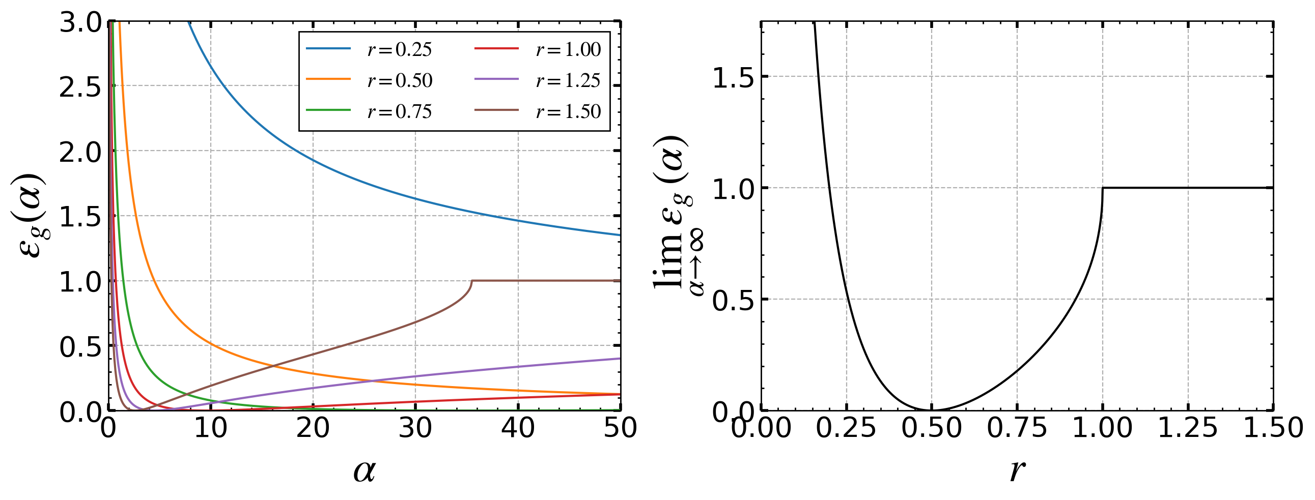
Figure 1: (Left) Generalizatioin error as a function of sample complexity $\alpha$ for different values of the ratio $r$. (Right) Asymptotic generalization error $\lim_{\alpha\to\infty}\varepsilon(\alpha)$ as a function of the the ratio $r$.

Learning Curve

For simplicity, we set $\tilde{\alpha}=r\alpha$ and $\lambda=\tilde{\lambda}=\eta=\tilde{\eta}=1$. Our analysis focuses on how the generalization error depends on $\alpha$ while varying the ratio $r$, as generating fake data from the generator is generally much easier than collecting real data. Fig. 1 (Left) shows the dependence of generalization error on sample complexity $\alpha$ for various values of the ratio $r$. The results demonstrate a sharp decline in the generalization error as the ratio $r$ increases. However, when $r$ becomes large, the generalization error increases in the region where $\alpha$ is large, eventually leading to a phase where no learning occurs, and the generalization error equals $1$. This implies that as $\alpha$ increases, the learning becomes dominated by only fake data.

In contrast, for smaller $r$, real data consistently dominates the objective function $V({\bm{w}},{\bm{v}};{\mathcal{D}},\tilde{{\mathcal{D}}})$, resulting in a steady decrease in generalization error. However, the reduced influence of the fake data component in the objective function, which drives the learning of the generator, requires a significantly larger amount of real data for effective generator training.

Asymptotic Generalisation Error

We next analyze the asymptotic behavior of the generalization error when the sample complexity $\alpha$ becomes sufficiently large. The asymptotic behavior of the generalization error as a function of $\alpha$ is given by

$$\varepsilon_{g}=\begin{cases}\frac{1-2\sqrt{\frac{1-r}{r}}r}{r}+\frac{2\sqrt{2}\left(\sqrt{\frac{1-r}{r}}r+r-1\right)}{(r-1)r\alpha^{1/2}}+{\mathcal{O}}(\alpha^{-1})&r\leq 1,\\ 1+{\mathcal{O}}(\alpha^{-1})&r>1.\end{cases}$$

The results for $\alpha\to\infty$ are shown in Fig. 1(Right). The optimal ratio is $r=\nicefrac{{1}}{{2}}$, indicating that using fake data approximately equal to half of the real data is effective when the dataset approaches infinity. At $r=1$, a phase transition occurs, suggesting that the model changes from a phase of effective learning phase to one where fake data becomes dominant. Beyond this point, for $r\geq 1$, the model fails to learn any meaningful signal ${\bm{w}}^{\ast}$, and the generalization error is $1$.

Furthermore, when $r=\nicefrac{{1}}{{2}}$, the generalization error scales as $\varepsilon_{g}\sim\alpha^{-1}$, which represents the optimal asymptotic behavior for a model-matched scenario. These results demonstrate the critical role of the ratio $r$ in determining learning performance. Therefore, tuning the ratio $r$ according to the available amount of real data is crucial for achieving optimal performance. In practice, it is known that in training GANs, the stability of learning can deteriorate depending on the ratio $r$ of fake to real data. This theoretical analysis provides insights into the importance of the ratio $r$ and is expected to contribute to improving learning algorithms.

5 Related Work

The replica method is a non-rigorous but powerful heuristic in statistical physics (Mézard et al., 1987; Mezard & Montanari, 2009; Edwards & Anderson, 1975). It has been proven to be a valuable method for high-dimensional machine-learning problems. Previous studies have investigated the relationship between dataset size and generalization error in supervised learning, including single-layer (Gardner & Derrida, 1988; Opper & Haussler, 1991; Barbier et al., 2019; Aubin et al., 2020) and multi-layer (Aubin et al., 2018) neural networks, as well as kernel methods(Dietrich et al., 1999; Bordelon et al., 2020; Gerace et al., 2020). In unsupervised learning, the replica method has also been applied to dimensionality reduction techniques such as the principal component analysis (Biehl & Mietzner, 1993; Hoyle & Rattray, 2004; 2007), and to generative models such as energy-based models (Decelle et al., 2018; Ichikawa & Hukushima, 2022) and denoising autoencoders (Cui & Zdeborová, 2023). However, the dataset-size dependence of GANs has not been previously analyzed, which this study aims to address. Similar to our work, a statistical mechanical formalism for addressing min-max problems has been proposed(Varga, 1998). However, the treatment of the inverse temperature limit differs from our approach, and it has limitations in accurately handling the order of the min and max operations.

6 Conclusion

This study introduces a statistical mechanical formalism to analyze high-dimensional min-max optimization problems, focusing on the critical order of min and max operations in non-convex scenarios. Our goal was to perform a sensitivity analysis of equilibrium values, providing new insights into their properties and generalization performance.

We applied this approach to a simple min-max game, evaluated the generalization performance of GANs, and derived the optimal ratio of fake to real data for effective learning. This successful application not only validates the approach but also opens the way for extending this formalism to more complex min-max problems and broader applications, suggesting a promising direction for significant advancements in machine learning and optimization.

Acknowledgments

We thank T. Takahashi, K. Okajima, Y. Nagano, and K. Nakaishi for useful discussions and suggestions. This work was supported by JST Grant Number JPMJPF2221 and JPSJ Grant-in-Aid for Scientific Research Number 23H01095. Additionally, YI was supported by the WINGS-FMSP program at the University of Tokyo.

Appendix A Derivation of Theorem 3.1 proof

In this section, we provide the derivation proof of Theorem 3.1. The derivation begins with the calculation of the free energy density without the analytic continuation of $p=-\beta_{\min}/\beta_{\max}$ to $p\in{\mathbb{N}}$. The free energy density in Eq. (2) is connected to the effective Hamiltonian, $\mathcal{H}_{\mathrm{eff}}({\bm{x}};{\bm{W}})$, which is defined through the relationship:

$$f(\beta_{\min},\beta_{\max};{\bm{W}})=-\frac{1}{\beta_{\min}d_{x}}{\mathbb{E}}_{A}\log\sum_{{\bm{x}}}\exp\left(-\beta_{\min}\mathcal{H}_{\mathrm{eff}}({\bm{x}};{\bm{W}})\right).$$

The effective Hamiltonian is given by

$${\mathcal{H}}_{\mathrm{eff}}({\bm{x}};{\bm{W}}) =\frac{1}{\beta_{\max}}\log\sum_{{\bm{y}}}e^{\beta_{\max}V({\bm{x}},{\bm{y}};{\bm{W}})},$$

$$=\frac{1}{\beta_{\max}}\log\sum_{{\bm{y}}}e^{\beta_{\max}\left(\frac{w_{xx}d_{x}}{2}\big{(}\frac{{\bm{x}}^{\top}{\bm{1}}_{d_{x}}}{d_{x}}\big{)}^{2}+\frac{d_{y}w_{yy}}{2}\big{(}\frac{{\bm{y}}^{\top}{\bm{1}}_{d_{y}}}{d_{y}}\big{)}^{2}+w_{xy}\sqrt{d_{x}d_{y}}\big{(}\frac{{\bm{x}}^{\top}{\bm{1}}_{d_{x}}}{d_{x}}\big{)}\big{(}\frac{{\bm{y}}^{\top}{\bm{1}}_{d_{y}}}{d_{y}}\big{)}\right)}$$

$$\times e^{\beta_{\max}\left(b_{x}d_{x}\big{(}\frac{{\bm{x}}^{\top}{\bm{1}}_{d_{x}}}{d_{x}}\big{)}+b_{y}d_{y}\big{(}\frac{{\bm{y}}^{\top}{\bm{1}}_{d_{y}}}{d_{y}}\big{)}\right)},$$

$$=\frac{1}{\beta_{\max}}\log e^{\beta_{\max}d_{x}\left(\frac{w_{xx}}{2}\big{(}\frac{{\bm{x}}^{\top}{\bm{1}}_{d_{x}}}{d_{x}}\big{)}^{2}+b_{x}\big{(}\frac{{\bm{x}}^{\top}{\bm{1}}_{d_{x}}}{d_{x}}\big{)}\right)}$$

$$\times\sum_{{\bm{y}}}e^{\beta_{\max}d_{y}\left(\frac{w_{yy}}{2}\big{(}\frac{{\bm{y}}^{\top}{\bm{1}}_{d_{y}}}{d_{y}}\big{)}^{2}+w_{xy}\sqrt{\frac{d_{x}}{d_{y}}}\big{(}\frac{{\bm{x}}^{\top}{\bm{1}}_{d_{x}}}{d_{x}}\big{)}\big{(}\frac{{\bm{y}}^{\top}{\bm{1}}_{d_{y}}}{d_{y}}\big{)}+b_{y}\big{(}\frac{{\bm{y}}^{\top}{\bm{1}}_{d_{y}}}{d_{y}}\big{)}\right)},$$

$$=\beta_{\max}d_{x}\left(\frac{w_{xx}d_{x}}{2}\left(\frac{{\bm{x}}^{\top}{\bm{1}}_{d_{x}}}{d_{x}}\right)^{2}+b_{x}d_{x}\left(\frac{{\bm{x}}^{\top}{\bm{1}}_{d_{x}}}{d_{x}}\right)\right)$$

$$\times\frac{1}{\beta_{\max}}\log\int d\hat{m}^{y}dm^{y}e^{\beta_{\max}d_{y}\left(\frac{w_{yy}}{2}(m^{y})^{2}+w_{xy}\sqrt{\frac{d_{x}}{d_{y}}}\big{(}\frac{{\bm{x}}^{\top}{\bm{1}}_{d_{x}}}{d_{x}}\big{)}m^{y}+b_{y}m^{y}-\frac{1}{\beta_{\max}}m^{y}\hat{m}^{y}+\frac{1}{\beta_{\max}}\mathrm{Softplus}(\hat{m}^{y})\right)+o(d_{y})},$$

where $\mathrm{Softplus}(x)=\log(1+e^{x})$. To evaluate the integral with respect to $\hat{m}^{y}$ and $m^{y}$, we take the limit as $d_{y}\to\infty$ and apply the saddle point approximation. The effective Hamiltonian can be expressed as follows:

$${\mathcal{H}}_{\mathrm{eff}}({\bm{x}};{\bm{W}})=d_{x}\Bigg{(}\frac{w_{xx}}{2}\left(\frac{{\bm{x}}^{\top}{\bm{1}}_{d_{x}}}{d_{x}}\right)^{2}+b_{x}\left(\frac{{\bm{x}}^{\top}{\bm{1}}_{d_{x}}}{d_{x}}\right)\\ +\kappa\underset{m^{y},\hat{m}^{y}}{\mathrm{extr}}\left[\frac{w_{yy}}{2}(m^{y})^{2}+w_{xy}\kappa^{-1/2}\left(\frac{{\bm{x}}^{\top}{\bm{1}}_{d_{x}}}{d_{x}}\right)m^{y}+b_{y}m^{y}-\frac{1}{\beta_{\max}}m^{y}\hat{m}^{y}+\frac{1}{\beta_{\max}}\mathrm{Softplus}(\hat{m}^{y})\right]\Bigg{)}.$$

where $\kappa=d_{y}/d_{x}$. By summing over ${\bm{x}}$, the free energy density can be calculated as follows:

$$f(\beta_{\min},\beta_{\max};{\bm{W}})$$

$$=-\frac{1}{\beta_{\min}d_{x}}\log\sum_{{\bm{x}}}e^{-\beta_{\min}d_{x}\left(\frac{w_{xx}}{2}\left(\frac{{\bm{x}}^{\top}{\bm{1}}_{d_{x}}}{d_{x}}\right)^{2}+b_{x}\left(\frac{{\bm{x}}^{\top}{\bm{1}}_{d_{x}}}{d_{x}}\right)\right)}$$

$$~{}~{}~{}~{}~{}~{}~{}~{}~{}~{}~{}\times e^{-\beta_{\min}d_{x}\left(\kappa\underset{m^{y},\hat{m}^{y}}{\mathrm{extr}}\left[\frac{w_{yy}}{2}(m^{y})^{2}+w_{xy}\kappa^{-1/2}\big{(}\frac{{\bm{x}}^{\top}{\bm{1}}_{d_{x}}}{d_{x}}\big{)}m^{y}+b_{y}m^{y}-\frac{1}{\beta_{\max}}m^{y}\hat{m}^{y}+\frac{1}{\beta_{\max}}\mathrm{Softplus}(\hat{m}^{y})\right]\right)},$$

$$=-\frac{1}{\beta_{\min}d_{x}}\log\left(\frac{d_{x}}{2\pi}\right)\int dm^{x}d\hat{m}^{x}e^{-\beta_{\min}d_{x}\left(\frac{w_{xx}}{2}(m^{x})^{2}+b_{x}m^{x}+\frac{1}{\beta_{\min}}m^{x}\hat{m}^{x}-\frac{1}{\beta_{\min}}\mathrm{Softplus}(\hat{m}^{x})\right)}$$

$$~{}~{}~{}~{}~{}~{}~{}~{}~{}~{}~{}\times e^{-\beta_{\min}d_{x}\left(\kappa\underset{m^{y},\hat{m}^{y}}{\mathrm{extr}}\left[\frac{w_{yy}}{2}(m^{y})^{2}+w_{xy}\kappa^{-1/2}m^{x}m^{y}+b_{y}m^{y}-\frac{1}{\beta_{\max}}m^{y}\hat{m}^{y}+\frac{1}{\beta_{\max}}\mathrm{Softplus}(\hat{m}^{y})\right]\right)},$$

$$=\underset{m^{x},\hat{m}^{x},m^{y},\hat{m}^{y}}{\mathrm{extr}}\Bigg{(}\frac{w_{xx}}{2}(m^{x})^{2}+b_{x}m^{x}+\frac{1}{\beta_{\min}}m^{x}\hat{m}^{x}-\frac{1}{\beta_{\min}}\mathrm{Softplus}(\hat{m}^{x})$$

$$~{}~{}~{}~{}~{}~{}~{}~{}~{}~{}+\frac{\kappa w_{yy}}{2}(m^{y})^{2}+w_{xy}\kappa^{1/2}m^{x}m^{y}+\kappa b_{y}m^{y}-\frac{\kappa}{\beta_{\max}}m^{y}\hat{m}^{y}+\frac{\kappa}{\beta_{\max}}\mathrm{Softplus}(\hat{m}^{y})\Bigg{)}.$$

The final equality is obtained by applying the saddle point method to evaluate the integral. From the saddle point equations, the following expressions are

$$m^{x}=\sigma(\hat{m}^{x}),~{}~{}m^{y}=\sigma(\hat{m}^{y})$$

Further transformation of the equation yields the following expression:

$$f(\beta_{\min},\beta_{\max};{\bm{W}})=\underset{m^{x},m^{y}}{\mathrm{extr}}\Bigg{[}\frac{w_{xx}}{2}(m^{x})^{2}+\frac{\kappa w_{yy}}{2}(m^{y})^{2}+w_{xy}\kappa^{1/2}m^{x}m^{y}+b_{x}m^{x}+\kappa b_{y}m^{y}-\frac{1}{\beta_{\min}}H(m^{x})+\frac{\kappa}{\beta_{\max}}H(m^{y})\Bigg{]},$$ (28)

where $H(x)=-x\log x-(1-x)\log(1-x)$ represents the binary cross-entropy.

Next, we proceed to evaluate the free energy density under analytic continuation in the replica method, which is expressed as

$$\hat{f}(\beta_{\min},\beta_{\max};{\bm{W}})=-\frac{1}{\beta_{\min}d_{x}}\log\sum_{{\bm{x}}}\sum_{{\bm{y}}_{1},\ldots,{\bm{y}}_{p}}e^{\beta_{\max}d_{x}\left(\frac{w_{xx}p}{2}\left(\frac{{\bm{x}}^{\top}{\bm{1}}_{d_{x}}}{d_{x}}\right)^{2}+\frac{\kappa w_{yy}}{2}\sum_{l}\left(\frac{{\bm{y}}_{l}^{\top}{\bm{1}}_{d_{y}}}{d_{y}}\right)^{2}\right)}\\ \times e^{\beta_{\max}d_{x}\left(w_{xy}\kappa^{1/2}\left(\frac{{\bm{x}}^{\top}{\bm{1}}_{d_{x}}}{d_{x}}\right)\sum_{l}\left(\frac{{\bm{y}}_{l}^{\top}{\bm{1}}_{d_{y}}}{d_{y}}\right)+b_{x}p\left(\frac{{\bm{x}}^{\top}{\bm{1}}_{d_{x}}}{d_{x}}\right)+\kappa b_{y}\sum_{l}\left(\frac{{\bm{y}}_{l}^{\top}{\bm{1}}_{d_{y}}}{d_{y}}\right)\right)}.$$

We introduce the order parameter through the Fourier transform representation of the delta function:

$$\hat{f}(\beta_{\min},\beta_{\max};{\bm{W}})$$

$$=-\frac{1}{\beta_{\min}d_{x}}\log\left(\frac{d_{x}d^{p}_{y}}{(2\pi)^{p+1}}\right)\int dm^{x}d\hat{m}^{x}\prod_{l}dm_{l}^{y}d\hat{m}_{l}^{y}e^{\beta_{\max}d_{x}\left(\frac{w_{xx}p}{2}(m^{x})^{2}+\frac{\kappa w_{yy}}{2}\sum_{l}(m^{y}_{l})^{2}+w_{xy}\kappa^{1/2}m^{x}\sum_{l}m_{l}^{y}\right)}$$

$$\times e^{\beta_{\max}d_{x}\left(b_{x}pm^{x}+\kappa b_{y}\sum_{l}m_{l}^{y}-\frac{1}{\beta_{\max}}\hat{m}^{x}m^{x}-\frac{\kappa}{\beta_{\max}}\sum_{l}\hat{m}^{y}_{l}m^{y}_{l}\right)}\sum_{{\bm{x}}}e^{\hat{m}^{x}\sum_{i}x_{i}}\sum_{{\bm{y}}_{1},\ldots,{\bm{y}}_{p}}e^{\sum_{l}\hat{m}_{l}^{y}\sum_{j}y_{j}},$$

$$=-\frac{1}{\beta_{\min}d_{x}}\log\left(\frac{d_{x}d^{p}_{y}}{(2\pi)^{p+1}}\right)\int dm^{x}d\hat{m}^{x}\prod_{l}dm_{l}^{y}d\hat{m}_{l}^{y}e^{\beta_{\max}d_{x}\left(\frac{w_{xx}p}{2}(m^{x})^{2}+\frac{\kappa w_{yy}}{2}\sum_{l}(m^{y}_{l})^{2}+w_{xy}\kappa^{1/2}m^{x}\sum_{l}m_{l}^{y}\right)}$$

$$\times e^{\beta_{\max}d_{x}\left(b_{x}pm^{x}+\kappa b_{y}\sum_{l}m_{l}^{y}-\frac{1}{\beta_{\max}}\hat{m}^{x}m^{x}-\frac{\kappa}{\beta_{\max}}\sum_{l}\hat{m}^{y}_{l}m^{y}_{l}+\frac{1}{\beta_{\max}}\mathrm{Softplus}(\hat{m}^{x})+\frac{\kappa}{\beta_{\max}}\sum_{l}\mathrm{Softplus}(\hat{m}_{l}^{y})\right)}.$$

Under the assumption of replica symmetry, where $\forall l\in[p],~{}~{}\hat{m}_{l}^{y}=m^{y},m_{l}^{y}=m^{y}$, we can further reformulate the expression as follows:

$$\hat{f}(\beta_{\min},\beta_{\max};{\bm{W}})$$

$$=-\frac{1}{\beta_{\min}d_{x}}\log\int dm^{x}d\hat{m}^{x}dm^{y}d\hat{m}^{y}e^{-\beta_{\min}d_{x}\left(\frac{w_{xx}}{2}(m^{x})^{2}+\frac{\kappa w_{yy}}{2}(m^{y})^{2}+w_{xy}\kappa^{1/2}m^{x}m^{y}\right)}$$

$$~{}~{}~{}~{}~{}~{}~{}~{}~{}~{}\times e^{-\beta_{\min}d_{x}\left(b_{x}m^{x}+\kappa b_{y}m^{y}-\frac{1}{\beta_{\max}p}\hat{m}^{x}m^{x}-\frac{\kappa}{\beta_{\max}}\hat{m}^{y}m^{y}+\frac{1}{\beta_{\max}p}\mathrm{Softplus}(\hat{m}^{x})+\frac{\kappa}{\beta_{\max}}\mathrm{Softplus}(\hat{m}^{y})+o(d^{x})+o(d^{y})\right)},$$

$$=\underset{m^{x},m^{y},\hat{m}^{x},\hat{m}^{y}}{\mathrm{extr}}\Bigg{[}\frac{w_{xx}}{2}(m^{x})^{2}+\frac{\kappa w_{yy}}{2}(m^{y})^{2}+w_{xy}\kappa^{1/2}m^{x}m^{y}+b_{x}m^{x}+\kappa b_{y}m^{y}$$

$$~{}~{}~{}~{}~{}~{}~{}~{}~{}-\frac{1}{\beta_{\max}p}\hat{m}^{x}m^{x}-\frac{\kappa}{\beta_{\max}}\hat{m}^{y}m^{y}+\frac{1}{\beta_{\max}p}\mathrm{Softplus}(\hat{m}^{x})+\frac{\kappa}{\beta_{\max}}\mathrm{Softplus}(\hat{m}^{y})\Bigg{]}.$$

The final equality is derived by handling the integral using the saddle point method. Consequently, the following saddle point equation is obtained:

$$m^{x} =\sigma(\hat{m}^{x}),~{}~{}m^{y}=\sigma(\hat{m}^{y}).$$

Substituting these results, the following expression for the free energy density is derived as

$$\hat{f}(\beta_{\min},\beta_{\max};{\bm{W}})=\underset{m^{x},m^{y}}{\mathrm{extr}}\Bigg{[}\frac{w_{xx}}{2}(m^{x})^{2}+\frac{\kappa w_{yy}}{2}(m^{y})^{2}+w_{xy}\kappa^{1/2}m^{x}m^{y}+b_{x}m^{x}+\kappa b_{y}m^{y}-\frac{1}{\beta_{\min}}H(m^{x})+\frac{\kappa}{\beta_{\max}}H(m^{y})\Bigg{]}.$$ (29)

This result coincides with the exact free energy density $f(\beta_{\min},\beta_{\max};{\bm{W}})$, derived without the need for analytic continuation.

References

- Arjovsky et al. (2017) Martin Arjovsky, Soumith Chintala, and Léon Bottou. Wasserstein generative adversarial networks. In International conference on machine learning, pp. 214–223. PMLR, 2017.
- Aubin et al. (2018) Benjamin Aubin, Antoine Maillard, Florent Krzakala, Nicolas Macris, Lenka Zdeborová, et al. The committee machine: Computational to statistical gaps in learning a two-layers neural network. Advances in Neural Information Processing Systems, 31, 2018.
- Aubin et al. (2020) Benjamin Aubin, Florent Krzakala, Yue Lu, and Lenka Zdeborová. Generalization error in high-dimensional perceptrons: Approaching bayes error with convex optimization. Advances in Neural Information Processing Systems, 33:12199–12210, 2020.
- Barbier et al. (2019) Jean Barbier, Florent Krzakala, Nicolas Macris, Léo Miolane, and Lenka Zdeborová. Optimal errors and phase transitions in high-dimensional generalized linear models. Proceedings of the National Academy of Sciences, 116(12):5451–5460, 2019.
- Biehl & Mietzner (1993) M Biehl and A Mietzner. Statistical mechanics of unsupervised learning. Europhysics Letters, 24(5):421, 1993.
- Bordelon et al. (2020) Blake Bordelon, Abdulkadir Canatar, and Cengiz Pehlevan. Spectrum dependent learning curves in kernel regression and wide neural networks. In International Conference on Machine Learning, pp. 1024–1034. PMLR, 2020.
- Bruck (1977) Ronald E Bruck. On the weak convergence of an ergodic iteration for the solution of variational inequalities for monotone operators in hilbert space. J. Math. Anal. Appl, 61(1):159–164, 1977.
- Cui & Zdeborová (2023) Hugo Cui and Lenka Zdeborová. High-dimensional asymptotics of denoising autoencoders. arXiv preprint arXiv:2305.11041, 2023.
- Daskalakis et al. (2017) Constantinos Daskalakis, Andrew Ilyas, Vasilis Syrgkanis, and Haoyang Zeng. Training gans with optimism. arXiv preprint arXiv:1711.00141, 2017.
- Decelle et al. (2018) Aurélien Decelle, Giancarlo Fissore, and Cyril Furtlehner. Thermodynamics of restricted boltzmann machines and related learning dynamics. Journal of Statistical Physics, 172:1576–1608, 2018.
- Dem’yanov & Pevnyi (1972) Vladimir Fedorovich Dem’yanov and Aleksandr Borisovich Pevnyi. Numerical methods for finding saddle points. USSR Computational Mathematics and Mathematical Physics, 12(5):11–52, 1972.
- Dietrich et al. (1999) Rainer Dietrich, Manfred Opper, and Haim Sompolinsky. Statistical mechanics of support vector networks. Physical review letters, 82(14):2975, 1999.
- Edwards & Anderson (1975) Samuel Frederick Edwards and Phil W Anderson. Theory of spin glasses. Journal of Physics F: Metal Physics, 5(5):965, 1975.
- Fontanari (1995) José Fernando Fontanari. A statistical analysis of the knapsack problem. Journal of Physics A: Mathematical and General, 28(17):4751, 1995.
- Freund & Schapire (1999) Yoav Freund and Robert E Schapire. Adaptive game playing using multiplicative weights. Games and Economic Behavior, 29(1-2):79–103, 1999.
- Gardner & Derrida (1988) Elizabeth Gardner and Bernard Derrida. Optimal storage properties of neural network models. Journal of Physics A: Mathematical and general, 21(1):271, 1988.
- Gerace et al. (2020) Federica Gerace, Bruno Loureiro, Florent Krzakala, Marc Mézard, and Lenka Zdeborová. Generalisation error in learning with random features and the hidden manifold model. In International Conference on Machine Learning, pp. 3452–3462. PMLR, 2020.
- Gidel et al. (2018) Gauthier Gidel, Hugo Berard, Gaëtan Vignoud, Pascal Vincent, and Simon Lacoste-Julien. A variational inequality perspective on generative adversarial networks. arXiv preprint arXiv:1802.10551, 2018.
- Gidel et al. (2019) Gauthier Gidel, Reyhane Askari Hemmat, Mohammad Pezeshki, Rémi Le Priol, Gabriel Huang, Simon Lacoste-Julien, and Ioannis Mitliagkas. Negative momentum for improved game dynamics. In The 22nd International Conference on Artificial Intelligence and Statistics, pp. 1802–1811. PMLR, 2019.
- Goodfellow et al. (2014a) Ian Goodfellow, Jean Pouget-Abadie, Mehdi Mirza, Bing Xu, David Warde-Farley, Sherjil Ozair, Aaron Courville, and Yoshua Bengio. Generative adversarial nets. Advances in neural information processing systems, 27, 2014a.
- Goodfellow et al. (2020) Ian Goodfellow, Jean Pouget-Abadie, Mehdi Mirza, Bing Xu, David Warde-Farley, Sherjil Ozair, Aaron Courville, and Yoshua Bengio. Generative adversarial networks. Communications of the ACM, 63(11):139–144, 2020.
- Goodfellow et al. (2014b) Ian J Goodfellow, Jonathon Shlens, and Christian Szegedy. Explaining and harnessing adversarial examples. arXiv preprint arXiv:1412.6572, 2014b.
- Hoyle & Rattray (2004) David C Hoyle and Magnus Rattray. Principal-component-analysis eigenvalue spectra from data with symmetry-breaking structure. Physical Review E, 69(2):026124, 2004.
- Hoyle & Rattray (2007) David C Hoyle and Magnus Rattray. Statistical mechanics of learning multiple orthogonal signals: asymptotic theory and fluctuation effects. Physical review E, 75(1):016101, 2007.
- Ichikawa & Hukushima (2022) Yuma Ichikawa and Koji Hukushima. Statistical-mechanical study of deep boltzmann machine given weight parameters after training by singular value decomposition. Journal of the Physical Society of Japan, 91(11):114001, 2022.
- Ichikawa & Hukushima (2023) Yuma Ichikawa and Koji Hukushima. Dataset size dependence of rate-distortion curve and threshold of posterior collapse in linear vae. arXiv preprint arXiv:2309.07663, 2023.
- Ichikawa & Hukushima (2024) Yuma Ichikawa and Koji Hukushima. Learning dynamics in linear VAE: Posterior collapse threshold, superfluous latent space pitfalls, and speedup with KL annealing. In Sanjoy Dasgupta, Stephan Mandt, and Yingzhen Li (eds.), Proceedings of The 27th International Conference on Artificial Intelligence and Statistics, volume 238 of Proceedings of Machine Learning Research, pp. 1936–1944. PMLR, 02–04 May 2024. URL https://proceedings.mlr.press/v238/ichikawa24a.html.
- Ipsen & Hansen (2019) Niels Ipsen and Lars Kai Hansen. Phase transition in pca with missing data: Reduced signal-to-noise ratio, not sample size! In International Conference on Machine Learning, pp. 2951–2960. PMLR, 2019.
- Isola et al. (2017) Phillip Isola, Jun-Yan Zhu, Tinghui Zhou, and Alexei A Efros. Image-to-image translation with conditional adversarial networks. In Proceedings of the IEEE conference on computer vision and pattern recognition, pp. 1125–1134, 2017.
- Ledig et al. (2017) Christian Ledig, Lucas Theis, Ferenc Huszár, Jose Caballero, Andrew Cunningham, Alejandro Acosta, Andrew Aitken, Alykhan Tejani, Johannes Totz, Zehan Wang, et al. Photo-realistic single image super-resolution using a generative adversarial network. In Proceedings of the IEEE conference on computer vision and pattern recognition, pp. 4681–4690, 2017.
- Lesieur et al. (2015) Thibault Lesieur, Florent Krzakala, and Lenka Zdeborová. Phase transitions in sparse pca. In 2015 IEEE International Symposium on Information Theory (ISIT), pp. 1635–1639. IEEE, 2015.
- Liang & Stokes (2019) Tengyuan Liang and James Stokes. Interaction matters: A note on non-asymptotic local convergence of generative adversarial networks. In The 22nd International Conference on Artificial Intelligence and Statistics, pp. 907–915. PMLR, 2019.
- Lions (1978) Pierre-Louis Lions. Une méthode itérative de résolution d’une inéquation variationnelle. Israel Journal of Mathematics, 31:204–208, 1978.
- Lucic et al. (2018) Mario Lucic, Karol Kurach, Marcin Michalski, Sylvain Gelly, and Olivier Bousquet. Are gans created equal? a large-scale study. Advances in neural information processing systems, 31, 2018.
- Madry et al. (2017) Aleksander Madry, Aleksandar Makelov, Ludwig Schmidt, Dimitris Tsipras, and Adrian Vladu. Towards deep learning models resistant to adversarial attacks. arXiv preprint arXiv:1706.06083, 2017.
- Maistroskii (1977) D Maistroskii. Gradient methods for finding saddle points. Matekon, 13(3):22, 1977.
- Mezard & Montanari (2009) Marc Mezard and Andrea Montanari. Information, physics, and computation. Oxford University Press, 2009.
- Mézard & Parisi (1986) Marc Mézard and Giorgio Parisi. A replica analysis of the travelling salesman problem. Journal de physique, 47(8):1285–1296, 1986.
- Mézard et al. (1987) Marc Mézard, Giorgio Parisi, and Miguel Angel Virasoro. Spin glass theory and beyond: An Introduction to the Replica Method and Its Applications, volume 9. World Scientific Publishing Company, 1987.
- Nemirovsky et al. (1983) AS Nemirovsky, DB Yudin, and ER DAWSON. Wiley-interscience series in discrete mathematics, 1983.
- Opper & Haussler (1991) Manfred Opper and David Haussler. Generalization performance of bayes optimal classification algorithm for learning a perceptron. Physical Review Letters, 66(20):2677, 1991.
- Papernot et al. (2016) Nicolas Papernot, Patrick McDaniel, Somesh Jha, Matt Fredrikson, Z Berkay Celik, and Ananthram Swami. The limitations of deep learning in adversarial settings. In 2016 IEEE European symposium on security and privacy (EuroS&P), pp. 372–387. IEEE, 2016.
- Potters & Bouchaud (2020) Marc Potters and Jean-Philippe Bouchaud. A First Course in Random Matrix Theory: For Physicists, Engineers and Data Scientists. Cambridge University Press, 2020.
- Reed et al. (2016) Scott Reed, Zeynep Akata, Xinchen Yan, Lajanugen Logeswaran, Bernt Schiele, and Honglak Lee. Generative adversarial text to image synthesis. In International conference on machine learning, pp. 1060–1069. PMLR, 2016.
- Refinetti & Goldt (2022) Maria Refinetti and Sebastian Goldt. The dynamics of representation learning in shallow, non-linear autoencoders. In International Conference on Machine Learning, pp. 18499–18519. PMLR, 2022.
- Szegedy et al. (2013) Christian Szegedy, Wojciech Zaremba, Ilya Sutskever, Joan Bruna, Dumitru Erhan, Ian Goodfellow, and Rob Fergus. Intriguing properties of neural networks. arXiv preprint arXiv:1312.6199, 2013.
- Takahashi & Kabashima (2022) Takashi Takahashi and Yoshiyuki Kabashima. Macroscopic analysis of vector approximate message passing in a model-mismatched setting. IEEE Transactions on Information Theory, 68(8):5579–5600, 2022.
- Tseng (1995) Paul Tseng. On linear convergence of iterative methods for the variational inequality problem. Journal of Computational and Applied Mathematics, 60(1-2):237–252, 1995.
- Varga (1998) Peter Varga. Minimax games, spin glasses, and the polynomial-time hierarchy of complexity classes. Physical Review E, 57(6):6487, 1998.
- Von Neumann & Morgenstern (2007) John Von Neumann and Oskar Morgenstern. Theory of games and economic behavior: 60th anniversary commemorative edition. In Theory of games and economic behavior. Princeton university press, 2007.
- Wald (1945) Abraham Wald. Statistical decision functions which minimize the maximum risk. Annals of Mathematics, 46(2):265–280, 1945.
- Wang et al. (2019) Chuang Wang, Hong Hu, and Yue Lu. A solvable high-dimensional model of gan. Advances in Neural Information Processing Systems, 32, 2019.
- Wishart (1928) John Wishart. The generalised product moment distribution in samples from a normal multivariate population. Biometrika, pp. 32–52, 1928.