Network evolution with Macroscopic Delays: asymptotics and condensation
Abstract.
Driven by the explosion of data and the impact of real-world networks, a wide array of mathematical models have been proposed to understand the structure and evolution of such systems, especially in the temporal context. Recent advances in areas such as distributed cyber-security and social networks have motivated the development of probabilistic models of evolution where individuals have only partial information on the state of the network when deciding on their actions. This paper aims to understand models incorporating network delay, where new individuals have information on a time-delayed snapshot of the system. We consider the setting where one has macroscopic delays, that is, the “information” available to new individuals is the structure of the network at a past time, which scales proportionally with the current time and vertices connect using standard preferential attachment type dynamics. We obtain the local weak limit for the network as its size grows and connect it to a novel continuous-time branching process where the associated point process of reproductions has memory of the entire past. A more tractable ‘dual description’ of this branching process using an ‘edge copying mechanism’ is used to obtain degree distribution asymptotics as well as necessary and sufficient conditions for condensation, where the mass of the degree distribution “escapes to infinity”. We conclude by studying the impact of the delay distribution on macroscopic functionals such as the root degree.
Key words and phrases:
temporal networks, delay distribution, continuous time branching processes, random trees, stable age distribution theory, local weak convergence, coupling, renewal theory2020 Mathematics Subject Classification:
Primary: 60K35, 05C801. Introduction
Driven by the explosion in the amount of data on various real-world networks, the last few years have seen the development of a number of new mathematical network models to understand the emergence of macroscopic properties in such systems, the evolution of these systems over time, and the behavior of dynamic processes such as random walk explorations or epidemic models. See [albert2002statistical, newman2003structure, newman2010networks, bollobas2001random, durrett-rg-book, van2009random] and the references therein for an initial foray into these developments.
One area of increasing importance is dynamic or temporal networks, [holme2012temporal, masuda2016guidance], which play a fundamental role in many sociological and scientific disciplines. This includes the impact of such dynamics on information diffusion across social networks, such as the spread of malicious information on social networks [shah2012rumor], the role of heterogeneity in edge creation across different attribute groups, temporal network evolution and popularity bias in ascribing positional advantages in networks [wagner2017sampling, espin2018towards, antunes2023learning], driving downstream co-evolution of the dynamics of the network with algorithms such as recommendation systems, or the evolution of interaction networks in systems biology [navlakha2011network, young2018network]. Models of network evolution have played an essential role in understanding such questions, including mechanistic reasons for the emergence of empirically observed properties of these systems such as heavy-tailed degree distribution [albert2002statistical, barabasi1999emergence], the efficacy of seed reconstruction algorithms [bubeck-mossel, bubeck2017finding, banerjee2020persistence] and bias of network sampling and ranking algorithms [wagner2017sampling, karimi2022minorities, karimi2018homophily, antunes2023learning].
One major class of network evolution models assumes new vertices enter the system and then make probabilistic choices for connecting to existing vertices based on the entire current state of the network. A largely unexplored direction is the effect of limited information availability of the state of the system for new individuals trying to form connections. This has motivated (at least) two distinct lines of new research:
-
a)
Network evolution schemes where individuals try to form connections via local exploration schemes starting from random locations in the network [krapvisky2023magic, banerjee2022co].
-
b)
Most relevant for this work, incorporating network delay as a mechanism for information limitation. Recent work in this direction includes network delay and queuing network dynamics and their connection to unimodularity [baccelli2019renewal], the impact of time delay on the evolution of distributed ledgers [king2021fluid] and evolution of longest paths and one-endedness or lack-thereof of such systems [dey2022asymptotic].
Let us now describe the precise model of interest for this paper, initially restricting to the tree network setting and commenting on the more general setting subsequently. We will first describe the general network model and then specify the setting considered in this paper.
1.1. Network evolution with delay
The model has three ingredients:
-
a)
A time scale parameter . For reasons that will become evident below, the regime will be referred to as the macroscopic delay regime and is the main content of this paper; other regimes (referred to as the mesoscopic regime) will be studied in a companion paper [BBDS04_meso].
-
b)
A delay distribution on . In the regime, we can assume that is supported on without loss of generality.
-
c)
An attachment function , measuring the attractiveness of individuals based on their local information, assumed to be strictly positive.
Definition 1.1 (Network evolution with delay).
We grow a sequence of random trees as follows:
-
i)
The initial tree consists of a single vertex . At time , the tree consists of two vertices, labeled as and attached by a single edge directed from to . Call the vertex as the “root” of the tree.
-
ii)
Suppose the network has been constructed till time for . Let the vertices in be labeled as with edges directed from children to parent. For vertex (which entered the system at time ) and , let denote the degree of at time (which for all vertices other than the root is equal to the in-degree ) interpreted in various applications as a measure of trust accumulated till time . Initialize always with .
-
iii)
At time , a new vertex enters the system. A normalized time delay independent of is sampled. The information available to is the graph
-
iv)
Conditional on , this new vertex attaches to a vertex with probability proportional to
Write for the corresponding sequence of growing random trees and let denote the corresponding probability distribution of the sequence of growing random trees.
For notational convenience later, we will let and set for . In the evolution dynamics above, vertex only has the information of the state of the process , including the vertex set only at this time and their corresponding degree information (not the full degree information at time ). Call the vertex that attaches to as the “parent” of and direct the edge from to this parent resulting in the tree . Thus, for any , is a random tree on labelled vertices rooted at . In the sequel, to reduce notational overhead, we will drop the “integer part” . To keep this paper to a manageable length, we focus on the tree-network setting, deferring further discussion of potential extensions to the non-tree setting, related work, as well as open problems to Section 6.
The main goal of this paper is to study the regime with affine attachment functions. This corresponds to the setting where the delay is of the same order as the size of the network and thus is referred to as the macroscopic delay regime. Here (by assumption, a random variable ) can be interpreted as the “density” of information available to the vertex entering the system at that time. As mentioned above, the mesoscopic regime is considered in [BBDS04_meso].
1.2. Rationale for the paper and overview of our results
A formal background for and statements of the main results are developed in the next three Sections. Here we paraphrase some of the main contributions of this paper:
-
a)
Model formulation and novel probabilistic structures: While network evolution models using preferential attachment dynamics are now considered a fundamental tool-kit both for theoretical and applied frameworks for network analysis, models where individuals have limited information when making decisions, while quite natural, have been significantly less explored. One main goal of this paper is to formulate the delay model above and understand large network asymptotics for the model. We mainly focus on dynamics modulated by the linear (pure or affine) preferential attachment function so as to contrast the phenomena that emerge with the well explored setting without delay. The delay in this setting causes a fundamental change in both local and global functionals which should be contrasted to the mesoscopic regime in [BBDS04_meso] where under quite weak assumptions on the delay, the local limits are the same as the setting without delay. In the macroscopic regime, the local weak limit is described by (two different but equivalent) continuous-time branching processes. The first branching process, described in Section 3.1, tracks degree evolution via a limit point process resulting in an offspring distribution whose inter-arrival points are sequentially constructed through appropriate hazard functions that are dependent on all the previous inter-arrival times. Although this is a natural description, deriving explicit formulae from this representation turns out to be intractable owing to the non-trivial recursive dependencies between inter-arrival times. This challenge is circumvented using a second ‘dual’ description of this branching process where edges reproduce, see Section 3.3. This construction recovers a lot of ‘independence’ which enables application of core probabilistic tools in proving results about the limit object, in particular, quantifying limiting degree exponents and analyzing condensation phenomena (crowding) at the root.
-
b)
Novel degree exponent phenomena: Using the techniques developed, we show that if the delay distribution is supported on with , then the power law exponent is strictly heavier than the regime without delay, see Theorem 4.8. This is surprising as one might imagine, in the macroscopic regime, the flow of mass away from the bulk to vertices born early in the evolution of the network, would lead to a lighter tail. This is contrasted with a specific setting where , hence the root attracts a non-trivial density of edges, resulting in the power law exponent being strictly lighter than the setting without delay, see Corollary 4.2. One motivation for proving the local weak convergence results is that they imply asymptotics not just for local functionals, such as the degree distribution, but also for global functionals, such as the spectral distribution of the adjacency matrix, see Corollary 4.5.
-
c)
Condensation behavior: In the macroscopic delay regime, we give conditions for condensation type behavior where the mass of the degree distribution escapes to infinity, resulting in mean degree (in the tree regime) in the limit. This can equivalently be seen as the root attracting a non-trivial proportion of network vertices. Surprisingly, we show that this is only possible when , namely, each new vertex has a positive probability of attaching to the root, see Theorem 4.4.
-
d)
Tracking global functionals: In Theorem 4.11, we obtain the scaling behavior of the root degree as a prototype for a general approach to go from ‘local-to-global’ asymptotics. This involves refined quantification of the error in approximating the global dynamics by the branching process emerging in the local limit using renewal theory and coupling techniques.
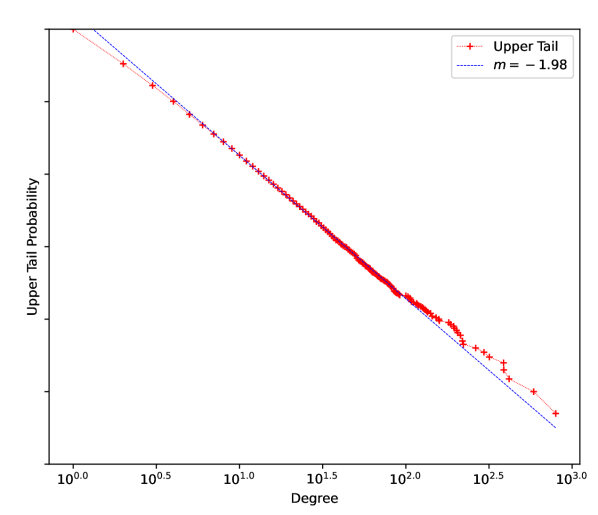
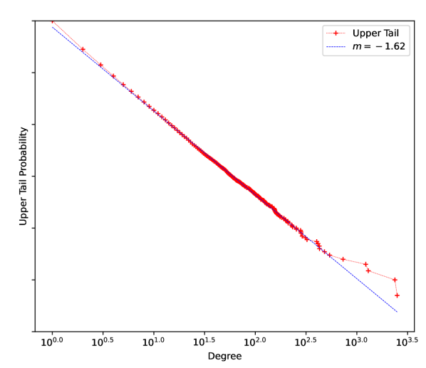
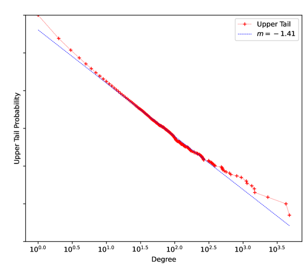
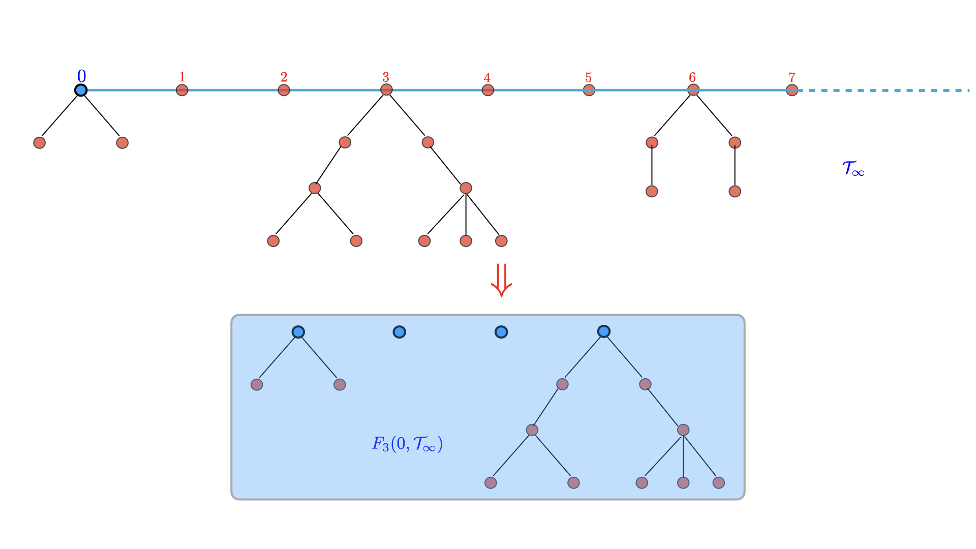
In Figure 1, we present simulated Preferential Attachment trees on nodes for different macroscopic delays. In Figure 2, the estimated upper tail exponent for the degree distribution is shown that matches with our result in Corollary 4.9.


1.3. Organization of the paper
In Section 2, we set up basic notation and definitions of local weak convergence. In Section 3, we describe the continuous time objects arising in the local limit for the macroscopic delay regime. Section 4 contains statements of the main results and also a brief overview of related work. Section 5 contains proofs of the main results. We conclude with open problems and potential extensions in Section 6.
2. Local weak convergence and sin-trees
One of the main goals of this paper is to prove that the sequence of random networks converges in an appropriate sense to limit infinite objects (setting this up in the context of trees versus general networks simplifies the exposition). The goal of this section is to describe now standard notions of such convergence, called local weak convergence [aldous-steele-obj, benjamini-schramm, van2023random]. We largely follow Aldous [aldous-fringe], which developed the foundations for local weak limits for probabilistic models of trees, where local weak convergence has an equivalent formulation in terms of convergence of fringe distribution of the sequence of random trees to corresponding objects for infinite trees with a single infinite path to infinity (sometimes referred to as sin-trees). The work of Aldous in [aldous-fringe] in the more involved setting of trees with vertex attributes was explained in [antunes2023attribute], this text we now paraphrase in our setting.
2.1. Mathematical notation
We use for stochastic domination between two real-valued probability measures. For let . If has an exponential distribution with rate , write this as . Write for the set of integers, for the real line, for the natural numbers and let . Write for convergence almost everywhere, in probability and in distribution, respectively. For a non-negative function , we write when is uniformly bounded, and when . Furthermore, write if and . We write that a sequence of events occurs with high probability (whp) when as . One of the core objects of this paper is the study of a sequence of growing random trees . Throughout we will write for the degree of the vertex in tree and write for the empirical degree counts,
| (1) |
2.2. Fringe decomposition for trees
For , let be the space of all rooted trees on vertices. Let be the space of all finite rooted trees. Here will be used to represent the empty tree (tree on zero vertices). Let denote the root of . For any and , let denote the subgraph of of vertices within graph distance from , viewed as an element of and rooted again at .
Given two rooted finite trees , say that if there exists a root preserving isomorphism between the two trees viewed as unlabelled graphs. Given two rooted trees ([benjamini-schramm], [van2023random]*Equation 2.3.15), define the distance
| (2) |
Next, fix a tree with root and a vertex at (graph) distance from the root. Let be the unique path from to . The tree can be decomposed as rooted trees , where is the tree rooted at , consisting of all vertices for which there exists a path from the root passing through . For , is the subtree rooted at , consisting of all vertices for which the path from the root passes through but not through , see Figure 3.
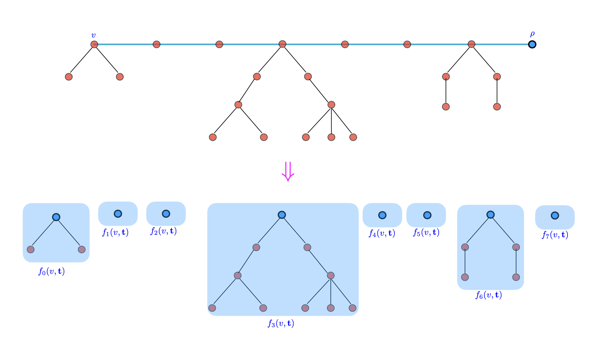
Call the map where , defined via,
as the fringe decomposition of about the vertex . Call the fringe of the tree at . For , call the extended fringe of the tree at truncated at distance from on the path to the root.
Now consider the space . The metric in (2) extends to , e.g., using the distance,
| (3) |
We can also define analogous extensions to for finite .
Next, an element , with for all , can be thought of as a locally finite infinite rooted tree with a single path to infinity (thus called a sin-tree [aldous-fringe]), as follows: Identify the sequence of roots of with the integer lattice , equipped with the natural nearest neighbor edge set, rooted at . Analogous to the definition of extended fringes for finite trees, for any , write . See Figure 4.
Call this the extended fringe of the tree at vertex , till distance , on the infinite path from . Call the fringe of the sin-tree . Now suppose is a probability measure on such that, for , a.s. . Then can be thought of as an infinite random sin-tree.
Define a matrix as follows: suppose the root in has degree , and let denote its children. For , let be the subtree below and rooted at , viewed as as an element of . Write,
| (4) |
Thus, counts the number of descendant subtrees of the root of that are isomorphic in the sense of topology to . If , define . Now consider a sequence of trees in such that fo all . Then there exists a unique infinite sin-tree with infinite path indexed by such that is the subtree rooted at for all . Conversely, it is easy to see, by taking to be the union of (vertices and induced edges) of for each , that every infinite sin-tree has such a representation. Following [aldous-fringe], we call this the monotone representation of the sin-tree .
2.2.1. Convergence on the space of trees
For , let denote the space of probability measures on the associated space, metrized using the topology of weak convergence inherited from the corresponding metric on the space , resulting in this space being a Polish space, see, e.g., [billingsley2013convergence]. Suppose be a sequence of finite rooted random trees on some common probability space (for notational convenience, assume , or more generally ). For and for each fixed , the empirical distribution of fringes up to distance
| (5) |
Thus can be viewed as a random sequence in and we can talk about weak convergence of this sequence, which is the content of (b) and (c) of the definition below. Further, with , define the probability measure on via the operation .
Definition 2.1 (Local weak convergence).
Fix a probability measure on .
-
a)
Say that a sequence of trees converges in expectation, in the fringe sense, to , if
Denote this convergence by as .
-
b)
Say that a sequence of trees converges in the probability sense, in the fringe sense, to , if
Denote this convergence by as .
-
c)
Say that a sequence of trees converges in probability, in the extended fringe sense, to a limiting infinite random sin-tree if for all one has
Denote this convergence by as .
In an identical fashion, one can define notions of convergence in distribution or almost surely in the fringe, respectively extended fringe sense. Letting denote the distribution of the fringe of on , convergence in (c) above clearly implies convergence in notion (b) with . More surprisingly, if the limiting distribution in (b) has a certain ‘stationarity’ property (defined below), convergence in the fringe sense implies convergence in the extended fringe sense as we now describe. Further, under an “extremality” condition of the limit objection in (a), convergence in expectation implies convergence in probability as in (b). We need the following definitions.
Definition 2.2 (Fringe distribution [aldous-fringe]).
Say that a probability measure on is a fringe distribution if
It is easy to check that the space of fringe distributions is a convex subspace of the space of probability measure on and thus one can talk about extreme points of this convex subspace. The following fundamental theorem is one of the highlights of [aldous-fringe].
Theorem 2.3 ([aldous-fringe]).
Fix a fringe distribution . Suppose a sequence of trees converges in the expected fringe sense as . If is extremal in the space of fringe measures, then the above convergence in expectation automatically implies .
The advantage of this result is that for proving convergence in the probability fringe sense, at least under the extremality of the limit object, dealing with expectations is enough. The next result shows that convergence in the probability fringe sense often automatically implies convergence to a limit infinite sin-tree. We need one additional definition. For any fringe distribution on , one can uniquely obtain the law of a random sin-tree with monotone decomposition such that for any , any in ,
| (6) |
where the product is taken to be one if . The following Lemma follows by adapting the proof of [aldous-fringe]*Propositions 10 and 11, and the proof is omitted.
Lemma 2.4.
Suppose a sequence of trees converges in probability, in the fringe sense, to . Moreover, suppose that is a fringe distribution in the sense of Definition 2.2. Then converges in probability, in the extended fringe sense, to a limiting infinite random sin-tree whose law is uniquely obtained from via (6).
Fringe convergence and extended fringe convergence imply convergence of functionals, such as the degree distribution. For example, letting with root denoted by say, convergence in notion (b) in particular implies that for any ,
| (7) |
However, both convergences give much more information about the asymptotic properties of beyond its degree distribution.
3. Limit objects for Macroscopic delays
3.1. A branching process driven by point processes with memory
In the setting of macroscopic delays, we restrict ourselves to the affine Preferential attachment setting with attachment function for , for a fixed parameter . We will write the corresponding model in Definition 1.1 as , where now the delay distribution is supported on . In the construction of the continuous-time branching process [jagers-ctbp-book, jagers-nerman-1, jagers-nerman-2], one formulation is via describing a point process with inter-arrival times , where for each , conceptually (in the branching process) has the interpretation as the amount of time for a vertex to go from having to children. We will now specify a point process via recursive construction of its inter-arrival times. Recall the delay distribution random variable from Definition 1.1. Define random variable by,
| (8) |
Note that corresponds to the event . Let , with . The construction proceeds as follows:
-
a)
Base case : Define the hazard function via,
(9) Let be the random variable on with the above hazard rate so that for any , .
-
b)
General case (general ): Having constructed , conditional on the above sequence, consider the hazard function for ,
(10) Let a.s. be the random variable with the above hazard rate.
The following gives a simpler representation of the above hazard rates, which can be easily verified from the definition.
Lemma 3.1.
Let . Then,
As shown in Theorem 4.1, the local weak limit of our network model is given by a branching process, with reproductions driven by , stopped at an independent exponential time. We now define these objects.
Definition 3.2 (BP in the Macroscopic regime).
Let be a continuous-time branching process started with one individual at time , where each individual has offspring distribution defined above. Let be an random variable, independent of , and write for the distribution of , viewed as a random finite rooted tree on , where we retain only genealogical information between individuals in .
3.2. Intuition for the limit object:
Before formally exhibiting the local weak limit, we give an intuitive picture of why the above continuous-time branching process is expected to show up in local asymptotics. To simplify notation, assume throughout. Let us start by considering a “continuous time” analog of the network process (without asserting that the discrete-time model of interest can be directly embedded into this process). Start with one vertex at time . Suppose at any given time , each vertex begets a new vertex at rate one. This new vertex is not necessarily a child of ; rather, it will connect to a vertex in after being provided a delay in the information available, namely the state of the system at time , which it will use to connect with probability proportional to the degree of the vertices in , where is independent of with distribution .
The first question is the relationship between the delay distribution and the original distribution . The dynamics of imply that the size of the process has the same distribution as a rate one Yule process; standard results about the Yule process imply that where . Now recall the discussion below Definition 1.1 where we suggested the interpretation of in the macroscopic regime as the density of information available to the new vertex. Thus, heuristically, one should have,
where the last approximation holds via the asymptotics for the Yule process. This gives explaining the transformation in (8). Further, let denote a randomly selected vertex in , born at time . Then its age by time satisfies,
| (11) |
This explains the origin of the random variable in Definition 3.2 describing the limit of the fringe distribution as run for an exponential rate one amount of time.
Now fix a large time and suppose a vertex was born into the system at time . Let us now, at least heuristically, try to get a handle on the evolution of its degree, starting from the transition from degree one (leaf) to degree two via a new vertex attaching to it. Fix and let us consider the hazard rate of a new vertex connecting to vertex at time , namely conditional on no connections to till this time, the probability of a new connection forming in the time interval . Call the set of new individuals born in this interval as . The approximate size, via the description of the dynamics of each individual reproducing at rate one, is . Each experiences an independent delay with distribution . Conditional on this delay, the probability of this new vertex connecting to is , where the numerator corresponds to the requirement that the delay should be such that information on vertex is available to . In contrast, the denominator corresponds to the total number of edges in the system corresponding to the information has. Laws of large numbers and Poisson approximation suggest that the probability of connection to at time after the birth of , given no connections till this time, is given by,
where once again we have used that for large , . This (and similar analysis for transition times to higher degrees) gives one explanation for the formulae for the hazard rates in (9) and (10).
3.3. Alternate description of using edge branching process
Consider the branching process in Def. 3.2 (we will suppress the dependence on to ease notation). Let denote the process representing the number of children of the root, namely for any , . By Theorem 4.1 below, the limit degree distribution is just the p.m.f of the random variable where independent of . Handling and directly using the hazard rate descriptions in (9) and (10) is hard as the inter-arrival times of are dependent in a highly non-trivial way rendering conventional branching process theory inapplicable. A key insight that we present now is a ‘dual’ description of the branching process in terms of another branching process where the edges reproduce. As we will see later, this construction uncovers a certain amount of independence in , thereby making it amenable to powerful branching process techniques.
Let us first explain the origin of this construction in the no-delay model where the network evolves using “pure” preferential attachment, i.e., a new vertex enters the system at each discrete time step and attaches to an existing vertex with probability proportional to the degree of the existing vertex. It is well known (e.g., [krapivsky2005network, vazquez2003growing]) that this model is equivalent to the following edge-copying model (see Figure 6):
-
a)
At each stage, a new vertex enters the system and picks an edge in the existing graph uniformly at random to copy. Thus, conceptually, we can think of each edge reproducing at rate one, independent across edges.
-
b)
Suppose the edge selected to copy is . Then attaches to with probability and with probability .
The dynamics above can be modified to incorporate affine attachment functions as well. It turns out, at least in the limit, one can construct similar dynamics in the delay regime, which allows significantly more tractable expressions for functionals of interest. The rest of this Section is organized as follows:
-
i)
We will describe an edge branching process for the general macroscopic delay model with affine preferential attachment function with parameter .
-
ii)
The offspring (children/immediate descendants) of can be constructed using a simpler primitive branching process and a Poisson process modulated immigration process .
Definition 3.3 (Edge branching process ).
Consider the following branching process :
-
(A)
At time , the population consists of two individuals connected by an edge directed from (child) to (parent).
-
(B)
At time units after its birth, an existing edge reproduces according to an inhomogeneous Poisson point process with rate , giving birth to a new edge (and thereby, a new individual) in the system.
-
(C)
At each reproduction epoch of edge , the resulting new edge attaches to the parent vertex of with probability and to the child of with probability .
Denote by the entire set of descendants of at time . Further let denote the number of children (immediate descendants) of by time .
Besides the description of as a more conventional continuous-time branching process (without complex hazard rates), the added advantage of the above construction is that the degree of the root (and thus any other vertex) in this branching process evolves as the size of another branching process with immigration.
Recall the hazard rate function (9). We will let denote the Poisson point process on with intensity measure,
| (12) |
-
a)
Let denote a (continuous time) branching process started with one individual at time and with offspring distribution . Let be iid copies of with respective sizes given by .
- b)
Consider the branching process with immigration , starting with one individual, where the progeny of each existing individual grows according to (an independent copy of) , and there is an additional incoming stream of individuals into the population at epochs of . The size of this branching process is thus given by
| (13) |
Proposition 3.4.
We have the distributional equivalence
| (14) |
Thus, Consequently, and, writing for the limit degree random variable in Theorem 4.1 with distribution , , where independent of .
Proof.
To prove the Proposition, it suffices to show (14) along with the independence of reproduction point processes across individuals in . The last distributional equality is immediate from rate considerations of the associated Poisson point processes. We will now show that the first and third objects in (14) have the same law.
Write for the times of arrival of new individuals into the branching process starting with when the root of is the only vertex in the system. Write for the interarrival time for the branching process between the -th and -th individual. Then, directly from construction, it is easy to check that for any ,
| (15) |
Comparing this to the hazard rates for in Section 3.1 and using Lemma 3.1 completes the proof. The independence of birth processes across individuals also follows via similar rate considerations.
The above construction will play a crucial role in proving all the main results related to degree distribution tail behavior and analyzing condensation phenomena at the root, which are formally stated in Section 4.
4. Main results
For the rest of this paper, regime and the model uses linear attachment with fixed affine parameter . Further, we assume that (else one is in the no-delay regime) and , else all arriving vertices just directly attach to the root. Recall that in the setting without delay, the limit degree distribution of the model (with associated degree exponent) is given by [bollobas2001degree, bollobas2003directed, barabasi1999emergence]:
| (16) |
As we describe the main results, the above can be viewed as something to compare and contrast in the setting with macroscopic delays.
4.1. Formal statement of results
We now give precise statements of our results. Recall, as before, from (1) that for , denotes the number of nodes in with degree exactly .
Theorem 4.1 (Local weak limit, macroscopic regime).
Consider the sequence of random trees in the macroscopic regime with affine linear attachment function and delay distribution on . Then converge in the expected fringe sense (Def. 2.1 (a)) to as in Definition 3.2. In particular, the degree distribution satisfies,
where is a rate one exponential random variable independent of .
One illustrative special case is the following, where one vacillates between complete information and no information (thus connecting directly to the root).
Corollary 4.2.
Fix and suppose the delay distribution . Then, for , the limit degree distribution is given by
for a constant . In particular, the degree exponent is strictly lighter than the regime with no delay.
The reader can compare this result with known results in the no-delay setting in (16). Surprisingly, under a wide array of settings, if there is no mass at one (i.e., no “trivial” mechanism for root connectivity), we will see that the degree exponent is always heavier than the model without delay. To set the stage, we start with the following two questions to consider: (a) under what conditions can one improve the above convergence in the expected fringe sense to convergence in probability, and perhaps even convergence to a limiting infinite random sin-tree? (b) Assuming that as in Cor. 4.2, it is easy to see that this automatically implies that the root degree and thus the limit degree distribution in Theorem 4.1 satisfies ; what are general conditions under which condensation happens? We start by formalizing the notion of mass of the degree distribution “escaping to ”.
Definition 4.3 (Condensation).
In the setting of Theorem 4.1, say that condensation occurs if .
The next result says that, essentially, the only way for condensation to happen is via the trivial mechanism described above.
Theorem 4.4.
One reason for proving such results is that they imply even convergence of global functions. Let be the random tree as above and let denote the adjacency matrix of and let denote the eigen-values and of denote the empirical spectral distribution where denotes the Dirac delta function.
Corollary 4.5.
Under the assumptions of Theorem 4.4(b), there exists a deterministic distribution (whose specific form depends on the parameters ) such that . The limit distribution has an infinite set of atoms in .
The proof of this result follows directly by combining the extended fringe convergence in Theorem 4.4 with [bhamidi2012spectra]*Theorem 4.1.
The goal of the next few results is, in the setting where , to understand the tail behavior of the degree distribution. Without delay, the degree exponent, that is, the power-law rate of decay of the tail probabilities of the limiting degree distribution, is [barabasi1999emergence, bollobas2001degree]. In this case, with “older vertices” getting a higher chance to reinforce their degree, one might imagine that the limiting degree distribution (which gives the degree behavior of “younger vertices” near the fringe) should have lighter tails. In the setting of Corollary 4.2, this is seen to be true. However, when , we will see that the opposite is true; namely, one obtains heavier tails. As before, we will phrase our results in terms of the transformed delay distribution instead of the original distribution .
The edge branching process construction described in Section 3.3 will play a major role both in the proof of Theorem 4.4 and the analysis of the degree exponents below.
Recall the Poisson point process with intensity measure as in (12).
Assumption 4.6 ( condition).
Assume the MGF of the finite part of exists for some positive , namely for some . This implies there exists a unique solving the equation,
| (17) |
With the above , define the random variable . Assume
The following lemma connects to the distribution of and consequently gives a range for .
Lemma 4.7.
Proof.
We will use for the tail of the degree distribution.
Theorem 4.8 (Non-condensation regime).
Assume .
-
a)
Under Assumption 4.6, there exists constant such that . Since , the degree exponent is strictly smaller than the regime without delay (that is, the distribution tails are heavier).
-
b)
Further assume there exists such that . Then, there exists constant such that .
The above result leads to the following special cases.
Corollary 4.9 (Non-condensation, special cases).
For the following special cases of the delay distribution :
-
a)
Suppose i.e. in a bounded sub-interval of . Then there exist (distribution dependent) constants such that where is the unique solution of the equation in (17).
-
b)
Suppose with . Then (18) has a unique positive solution given by
(19) and . Moreover, if either (i) or (ii) , then . Here, are constants depending on .
Remark 4.10.
-
a)
In the setting (b) above, corresponds to original delay having distribution for . When , the delay distribution converges weakly to the Dirac mass at zero. This is exhibited in the observation as , that is, the degree exponent approaches , namely, the exponent for the affine preferential attachment model without delay.
-
b)
For , to obtain a matching upper bound for the degree distribution, one needs to somehow verify the moment condition of Theorem 4.8(b). We leave this as an open problem.
The final result describes the scaling of the root degree in the non-condensation regime, showing that the scaling exponent above for the degree also governs the evolution of more macroscopic functionals. The same scaling should carry over to the maximal degree in this setting, but we will leave this to future work. For notational simplicity, we only consider the case .
Theorem 4.11 (Non-condensation regime, root degree scaling).
Set . Consider the root degree . Assume has a density such that . The following hold under the Assumptions of Theorem 4.8 with as in (17):
-
a)
Upper bound: Assume for all . Then there exists such that for any ,
-
b)
Lower bound: Assume such that . Then there exist finite positive constants such that for any ,
Remark 4.12.
Section 5.4 describes an edge copying procedure in a similar vein as (but more involved than) Section 3.3, which encodes the global evolution of the network process . The proof of Theorem 4.11 relies on a detailed quantification of the error incurred in approximating this edge copying procedure by the edge branching process in Section 3.3. This is achieved using renewal theoretic and coupling techniques. Besides its utility in root degree evolution, we believe that this approach is of independent interest and can be used to furnish asymptotics of a host of other global network functionals, e.g., root PageRank [banerjee2022pagerank].
4.2. Related work
We placed this work in the general area of dynamic network models in Section 1. The goal of this Section is to discuss research that directly influences this paper. Aldous’s paper [aldous-fringe] heralded the now fundamental notion of local weak convergence to understand asymptotics for large discrete random structures; for more recent work on fringe distributions, see the survey [holmgren2017fringe]. Our proof techniques use stochastic approximation techniques to understand the historical evolution of subtrees, which was first used in the context of preferential attachment models (without delay) in [rudas2007random]. While there is limited work to date on models related to delays in the macroscopic regime, understanding probabilistic evolution schemes giving rise to condensation phenomenon in networks has spurred a lot of literature over the last few years starting with [bianconi2001bose], see for example [dereich2017, borgs2007first, bhamidi2012twitter, banerjee2022co]. In the probability community, the study of dynamic network models in the family studied in this paper, incorporating delay in their evolution, is still largely in its infancy; the closest papers are [baccelli2019renewal, king2021fluid, dey2022asymptotic].
5. Proofs
We start by proving local weak convergence in the macroscopic regime (Theorem 4.1) in Sections 5.1 and 5.2. Section 5.3 contains proofs of the characterization of the degree exponent where the edge branching process described in Section 3.3 will play a central role in understanding conditions for condensation and probabilistic fringe convergence (Theorem 4.4) as well as tail exponents in the non-condensation regime (Theorem 4.8). Starting in section 5.4 and the ensuing sections contain the proof of the maximal degree scaling (Theorem 4.11).
5.1. Proof of Local weak convergence: Theorem 4.1
For a vertex and , define to be the first time vertex has its -th child (and ) in the discrete time network process . For , we label the vertex entering the fringe of vertex (the progeny tree associated with vertex ) by i.e
and . For , let be the birth time of th child of th vertex in the fringe of vertex (note that and ), and
be the inter-arrival time in -scale. One can think of the above quantity as the ‘continuous time’ (if we encode vertex arrivals by epochs of a Yule process) elapsed for the degree of the th descendant of vertex to increase from to . These form a point process of reproduction times of vertices in the fringe of vertex . The following Lemma shows that the inter-arrival times for these point processes weakly converge to those of the point process described in Section 3.1 as . Further, the point processes associated with distinct vertices in the fringe become asymptotically independent.
Proposition 5.1.
Let be iid copies of defined in Section 3.1. Then, as ,
We now present an immediate corollary of Proposition 5.1, which is the key component in the proof of Theorem 4.1. Let denote a random variable independent of the network process .
Corollary 5.2.
Let be iid copies of and be an exponential random variable of rate independent of . Then
In the remainder of the section, we prove Theorem 4.1. The proof of Proposition 5.1 will be provided in the next section.
Proof of Theorem 4.1.
For any and , one can construct a unique rooted tree via the following temporal evolution: (a) the root is born at time , (b) for any , denotes the age of the th born vertex in the tree when its th child is born (with root being the th born vertex), (c) retain only those vertices with birth times . For , denote by the birth time of the th born vertex in , and let . Define . Then, it is clear that is continuous.
Now, consider the evolution of the network process in the logarithmic time scale, namely, assign the birth time of to and to for . For any and , the fringe of vertex in can be expressed as , where , . In particular, the fringe of a uniformly chosen vertex is given by . By Corollary 5.2, where , . Moreover, using Lemma 3.1 (also, by Proposition 3.4), . Hence, by the continuous mapping theorem, , which has the law . This implies the local weak convergence in the expected fringe sense.
The convergence of the (expected) empirical degree distribution is an immediate consequence of this local weak convergence.
5.2. Proof of Proposition 5.1:
This section is dedicated to the proof of Proposition 5.1. Throughout the section, we fix . We start by computing the joint density of . Recall that and . For any and , let
| (20) |
where and . Using these functions and the hazard rate description for the inter-arrival times in Section 3.1, we conclude that the joint density of is given by
| (21) |
Note that and are discontinuous at most at countably many points. Hence, the density is continuous almost surely on w.r.t. Lebesgue measure.
Now we prove
Let be continuous function with compact support for some . We show
| (22) |
We first express as an integral over and using a sequence of approximations to the law of we prove (22). We first develop some notation to express the distribution of .
Recall and defined at the beginning of Section 5.1. Note that the values of are determined by the values of . Thus, for , one can define , the values of on the event , as follows:
-
•
and for .
-
•
Given for , define
Also, define and - the values of inter-arrival times in -scale on the event .
On the event , an incoming vertex attaches to a vertex in the fringe of vertex only at times . Also, let and be the times when the fringe is inactive, meaning there are no attachments.
In the discrete-time network process , an incoming vertex can only attach to a single existing vertex in the network. So, we say is valid if all are distinct for and .
For and , let
| (23) |
Observe that is the probability that an incoming vertex at time attaches to the vertex in the fringe of vertex given the history up to time on the event . Note that the sum above runs over such that and hence the right-hand side depends only on the network run up to time . We then have
| (24) |
We now approximate using the following sequence of approximations.
-
(1)
We replace the terms in the first product in (5.2) by exponentials to get where
(25) - (2)
-
(3)
Finally, we approximate the sums of type with appearing in the exponent of the first term in (26) to get where
(28) where
(29)
An upper bound on errors made by each approximation is given by the following Lemma, whose proof is given in Appendix A.
Lemma 5.3.
Let be a bounded subset in . Then we have
for some constant independent of the set , and .
Completing the Proof of Proposition 5.1: By (5.2), we have
Therefore, by Lemma 5.3, we have
for some constant depending only on and where the support of is . Thus, to prove (22), it is sufficient to show
| (30) |
To compute the integral on LHS of (30), consider the transformation where the inter-arrival times are in exponential scale where we make the change of variables with . More precisely, for , we define the following:
-
•
Let .
-
•
For , given , let to be the value of when .
We define by
We compute the integral on LHS of (30) after applying the transformation (which, as we will see, is the ‘approximate’ inverse of the transformation ). Note that the function is piece-wise differentiable and bijective. Moreover, the matrix of partial derivatives of is lower-triangular (when it is defined). Therefore, the Jacobian of the transformation is
| (31) |
Let and . Then after the transformation, the integral on the LHS of (30) is
We first show that is uniformly bounded when (the support of ). Observe that . Moreover, for (with convention ), which gives . Therefore implies
Hence the support of the integrand on the right-hand side of the above display is contained in . Recalling defined in (27) and , we have for any ,
where , and we recall from (5.2). Combining this with (31), we obtain
| (32) |
Therefore, if , the LHS of (32), and hence , is uniformly bounded (over ). Also, from the definition of in (29) and in (5.2), we have . Since , we have using the bounds on obtained above that . Using this along with (32), we thus obtain
| (33) | ||||
| (34) |
where .
Moreover, the Lebesgue measure of the set converges to zero by the following Lemma. Proof is given in Appendix A.
Lemma 5.4.
Let be the Lebesgue measure on . Then, as ,
where .
Further, by (33), (34) and definition of in (28), we have on the set ,
Hence, by DCT, we have
The last line follows from the expression for joint density of in (21). This finishes the proof.
Proof of Corollary 4.2: We now briefly describe the proof of the special case considered in this Corollary where the delay has a Bernoulli distribution. The corresponding transform is given by . Thus, using Lemma 3.1, the hazard for is given as
Thus , independent across different . Thus the tail probability,
Using independence, the moment generating functions of exponential random variables, and algebraic manipulations complete the proof.
5.3. Characterization of condensation: Proof of Theorem 4.4:
We will start by using Proposition 3.4 to prove the following.
Lemma 5.5.
Proof.
By Prop. 3.4,
| (35) |
where the fourth equality is a consequence of the memoryless property of exponential random variables.
Define . Using the forward decomposition of the branching process based on the reproduction times of the offspring of the root and their progeny sizes, one gets the standard renewal equation . Thus writing , the above identity gives and hence,
Now the term in the denominator,
| (36) |
and hence,
| (37) |
Moreover, as has rate
using (5.3). Using this and (37) in (5.3) completes the proof.
Completing the Proof of Theorem 4.4: Lemma 5.5 proves the characterization of condensation, namely Theorem 4.4(a), and further shows that if then the mean number of children of the root in the original branching process namely
By [aldous-fringe]*Proposition 3, is a fringe distribution in the sense of Definition 2.2. Moreover, by [aldous-fringe]*Theorem 13 (see also paragraph following the Theorem), is an extremal fringe distribution. Theorem 4.4(b) now follows from Theorem 2.3 and Lemma 2.4.
5.3.1. Tail exponents: Proof of Theorem 4.8 and Corollary 4.9:
Recall again, from Prop. 3.4, the characterization of the limit degree in terms of the total size of the edge branching process at a random time i.e. . We will use this to quantify the behavior of the tail exponents. We first start with some implications of the assumptions of (a) and (b) of Theorem 4.8.
Lemma 5.6.
Proof.
The parameter in (17) is the so-called Malthusian rate of growth of the edge branching process , which under the “” condition for continuous time branching processes implies , see [jagers-nerman-1, jagers-nerman-2, jagers-ctbp-book], where the limiting random variable is finite and strictly positive. In particular, . For , let denote the almost sure limit of as . Recall that the point process has rate and hence,
using the definition of .
Thus, writing , we conclude from the above observations that as . Moreover, gives, in particular, the (almost sure) finiteness of . Further,
The convergence to zero of the right-hand side above follows from the recorded observations along with the dominated convergence theorem and the independence of and .
To prove the second result, we first note by the equivalence of the existence of moments of and the corresponding moments of the normalized branching process, see [mori2019moments]*Theorem 4, that there exists such that
By Jensen’s inequality,
where we applied the independence of and in the second inequality. By rate considerations, the point process has the same law as . Hence,
by our assumption. The result follows from the above two displays.
Completing the proof of Theorem 4.8: Let us first prove part (a), namely the lower bound. By Lemma 5.6(a), there exist such that
| (38) |
Then for the degree distribution, for all , with ,
To prove (b), assume there exists such that . Using Lemma 5.6(b) and Markov’s inequality gives for any and ,
Thus,
This completes the proof of the Theorem.
Completing the proof of Corollary 4.9: Part (a) of Corollary 4.9 follows directly from Theorem 4.8. (19) in Corollary 4.9(b) follows by a straightforward algebraic manipulation. We omit the details. To prove the remaining claims of part (b), for any , ,
| (39) |
where the last step follows from Jensen’s inequality. Using the explicit form of the rate associated with the process and by standard moment bounds for Poisson random variables, for any , there exists (also depending on ) such that
Checking the assumptions of Theorem 4.8(a) for all values of (thereby giving the lower bound on the degree distribution) and those of Theorem 4.8(b) when (giving degree distribution upper bound) is now routine using the above and the observation . To check the moment condition of Theorem 4.8(b) when , , we use the Poisson moment bound above in (39) to obtain for any a constant such that
As we only need finiteness of the right-hand side for some , it suffices to show . Using the explicit formula of in (19), note that
which completes the proof.
5.4. Root degree behavior: Proof of Theorem 4.11:
Here, we consider the model with , and the goal is to prove Theorem 4.11. The proof of the root degree asymptotics relies on a careful quantification of the approximation of the network dynamics by that of the edge branching process described in Section 3.3, that extends beyond the ‘fringe’ (which the local limit captures) to the older vertices of the network evolution. First recall the “edge copying equivalence” of preferential attachment explained in Fig. 6. We describe a construction which is a natural extension to the delay regime.
Construction 5.7 (Copying construction of the delayed model).
Consider the following random tree model , started with a single edge and recursively constructed as follows:
-
a)
For assume the tree consists of vertex set and edge set in the order of attachment.
-
b)
With denoting the delay distribution as before, define the pmf ,
(40) -
c)
Copying procedure: To transition to , first select one of the edges using (i.e. selected with probability ). Suppose has been selected. Then is obtained from by adding a new vertex connected to with a new edge which is with probability or edge with probability .
The following is elementary to check.
Lemma 5.8.
Consider the delayed preferential attachment model with and delay distribution . As models of growing random trees, .
In order to understand the rate of growth of the root degree, essentially one needs to carefully understand the rate of copying events that involve the edges attached to the root .
Recall the intuition given in Section 3.2. To formalize this intuition, we will move Construction 5.7 into continuous time so that copying events happen at a rate proportional to the number of edges in the system. To do this, we first describe a continuous time analogue of the construction in in terms of time-changed Poisson processes. Let be iid Poisson rate one processes on . Consider the following evolution equations for :
| (41) |
where is the cdf of the delay variable . Since for any time , using the fact that the expression in (40) is a probability mass function, it is easy to check that . Thus it is easy to verify that is a rate one Yule process with . The above dynamics can be used to describe a growing network process by thinking of as the reproduction process of the -th added edge in continuous time as in Section 3.3. More precisely, consider the continuous time network process , started with , where the -th edge, added to the system at time reproduces, giving birth to new edges (equivalently, vertices) at the arrival times of . At each birth time, the new individual is connected to the parent vertex or child vertex of the -th edge with equal chance via an outgoing edge. Lemma 5.8 now implies that,
| (42) |
Although the above recipe provides a continuous time description of the entire discrete time process (not just the local weak limit), the rates appearing above have a substantially more complicated form than those for the edge branching process in Definition 3.3. In particular, the reproduction rates across different vertices are correlated through their mutual dependence on . However, using the approximations , and , we observe that
where we recall and . The right-hand side above looks exactly like the reproduction rates of the edge branching process in Definition 3.3 with some adjustment for the root.
In view of the above, a crucial technical ingredient is thus quantifying as a function of .
The following Lemma provides bounds on this quantity.
In the remainder of this section, we will denote by and the conditional probability and expectation given . We will write for . Also, will denote generic positive constants, not depending on , whose values might change between lines.
Lemma 5.9.
Assume has a density such that , and there exists such that . Then, for and , writing
we have
where the constants depend only on .
Note that the first bound in the Lemma has a better dependence on and a worse dependence on . The second bound has the reverse nature. As we will see later, the first bound will play a crucial role in the upper bound for the root degree while the second bound is required for the root degree lower bound.
In order to prove the above Lemma, we need some estimates about the Yule process recorded in the following Lemma. Proof is given in Appendix A.
Lemma 5.10.
Let be a rate one Yule process with and let . Then,
-
i)
For , . Moreover, is a -martingale and as , where and are iid random variables. Further,
-
ii)
-
iii)
.
-
iv)
For any , ,
Proof of Lemma 5.9.
First, note that
| (43) |
where
Now we will estimate the three errors above. Note that
| (44) |
To estimate the second term in the above bound, first note that
By Lemma 5.10(i),
Moreover, by Lemma 5.10(ii), there exists such that for all ,
Using these estimates, we obtain
Hence,
Using this in (5.4), we obtain
| (45) |
To estimate the second error term in (43), note that
| (46) |
By an application of Hölder’s inequality,
| (47) |
where we have used in the second inequality and in the third inequality. As for all ,
| (48) |
Now, using Lemma 5.10(i),
Moreover, to estimate the first term in the bound (5.4), note that by Lemma 5.10(i) and (ii),
Using this fact, we obtain
Using the above estimates in (5.4), we get
| (49) |
The second term in (5.4) can be estimated as in the first term in (5.4) to obtain
| (50) |
Using (49) and (50) in (5.4), we obtain
| (51) |
Similarly, using Lemma 5.10(ii) and (iii),
| (52) |
Hence, using (51) and (5.4) in (46), we obtain
| (53) |
Finally,
| (54) |
where we have used and the fact that . The first bound on in the lemma now follows upon using the estimates (45), (53) and (5.4) in (43).
To obtain the second bound, we will change the bound on by simply writing
Hence, by Lemma 5.10(iv), we obtain
which gives the second bound.
Completing the proof of upper bound in Theorem 4.11: For , let denote the degree of the root in at time and let . Then, writing , observe that
By Lemma 5.9,
Moreover, writing ,
and, using integration by parts,
Combining the above observations, we obtain
| (55) |
where . Now, define the measure on . By the definition of , is a probability measure. Hence, from (5.4), we obtain the following ‘renewal theoretic’ upper bound
where is the renewal measure associated with . Once again, using the definition of , it can be checked that
Moreover, recalling we can choose and fix large enough such that . This is allowed as by the assumed hypothesis of the Theorem. For this choice of ,
Further, by the assumption on finiteness of exponential moments, . Hence, by the key renewal theorem [jagers-ctbp-book], we obtain
| (56) |
Finally, we will translate the above bound for the root degree in the original discrete time network . Note that, by (42), . Therefore, for ,
Hence, from (56),
The upper bound in the Theorem now follows upon choosing .
5.5. Lower bound in Theorem 4.11:
For the lower bound, we construct a coupling between and the edge branching process described in Section 3.3. We denote the root of by . Recall the Ulam-Harris set , where . To describe the coupling, we will view the vertices in any growing tree process (with edges directed from child to parent) as -valued objects where the first coordinate encodes genealogical information and the second coordinate encodes birth time. For vertex , denote by the unique outgoing edge from . For , we will write to denote that is a child of , and to denote descends from (via a possible chain of ancestral edge reproductions). As before, and will respectively denote the conditional expectation and probability given the history of the network observed up to the birth time of vertex .
By (5.4), there is an independent rate one Poisson process associated with each encoding the times at which the edge gives birth. For , writing for the birth time of and for the chronological index of , define the event
Recall that the -th child of the edge in chooses to attach to or its parent vertex with equal chance. We denote the associated Bernoulli random variable as .
Fix . Intuitively we will think of large but fixed so that various functionals involved in the coupling have “stabilized’ in by the time it reaches time and one can potentially run two different coupled processes, one having dynamics modulated by the probabilistic rules in while the other run via the dynamics of , such that miscouplings can be handled.
The coupling: Let us now be more precise. The coupling involves the construction of a growing tree process which attempts to retain the maximal amount of genealogical and temporal information from while keeping the law of the reproduction point process of each edge born after time the same as that in . In the following, we say a vertex is copied from if there exist vertices in with the same values in as and its ancestors in . In this case, we will also use to denote the corresponding vertex in . Let denote the first vertex born into after time that attaches to the root . The construction is now described as follows:
-
i)
for all , that is, all vertices born into on this interval, along with their birth times and edges spanning them, are copied from onto . Moreover, copy all the vertices that are produced by reproduction of these edges.
-
ii)
For each vertex with birth time , the edge reproduces at times given by the epochs of and the newly born edges (equivalently, vertices) connect to or its parent vertex with equal chance. Moreover, if is copied, the -th newly born edge (equivalently, vertex) in the above point process connects to or its parent according to the value of the same Bernoulli variable governing the corresponding attachment in .
In other words, all children of vertices born before time in are copied onto and those born after time reproduce in a coupled way attempting to maximize the number of copied children on any compact time interval.
Note that if is copied and holds, then all the vertices originating from the reproduction of are copied as well.
Quantifying number of miscoupled vertices: Now, we will quantify the number of vertices in (born by a given time) which descend from , and which attach to the root in and have not been copied. We will call such vertices ‘miscoupled’. Define the following for :
In words, denotes the number of vertices in born up to time , descending from the edge , which attach to the root. denotes the number of copied vertices in born up to time , descending from the edge , which attach to the root. is the set of ‘bad’ vertices in in the sense that at least one of their children is not copied.
Observe that every vertex born in that is not copied descends from a vertex in . Hence, the number of miscoupled vertices in with birth times in is upper bounded by
Our proof of the root degree lower bound relies on the fact
| (57) |
We will quantify and show that, with high probability, it is much smaller than for large . This is achieved by the following Lemma.
Lemma 5.11.
Assume has a density such that , and there exists such that . There exists , such that for all and ,
The proof of the above Lemma involves viewing , for , as the size of the branching process introduced in Section 3.3 run up till time . An individual in this branching process can be marked as either ‘good’ or ‘bad’ depending on whether or not holds. Quantitative estimates on , derived from Lemma 5.9, are then used to bound the number of bad individuals via renewal theory.
We will need the following estimate for the Yule process whose proof is given in Appendix A.
Lemma 5.12.
For any , there exist positive constants depending on such that for all ,
Proof of Lemma 5.11.
For , define the subset of vertices
and the event
For any ,
| (58) |
By Markov’s inequality and Lemma 5.9 (this time requiring both bounds), for any ,
where the constants do not depend on . Hence, on the event ,
| (59) |
on choosing and fixing sufficiently small (the constants depend on ).
Moreover, by the assumed hypothesis , for all . From this and Jensen’s inequality, we conclude that which, by Lemma 5.6(b), gives
| (60) |
Using (59) and (60) in (58), we get
Now, as vertices in descend from , the above expectation can be bounded in terms of the birth times , where is the edge branching process determining root degree that was introduced in Section 3.3. Hence, we obtain
| (61) |
Writing , note that satisfies the following renewal-type equation
As and , we conclude and hence
Using this in (61) gives
| (62) |
Now, we bound . Note that, if for some copied with , we have , then
Completing the proof of lower bound in Theorem 4.11: All the constants appearing in the proof are independent of . By Lemma 5.6(b),
where is a strictly positive finite random variable.
Choose and fix such that , where is as in Lemma 5.11. As new vertices are added in according to a Yule process and a new vertex arriving at time attaches to the root with probability at least , it follows from this that the law of is stochastically dominated by . Hence,
From these observations and Fatou’s lemma, we conclude that for any ,
Let denote the first arrival time in the Poisson point process governing the edge branching process . Then it is straightforward to check that for any . By using the same argument as in the proof of [banerjee2023degree]*Lemma 3.5, we conclude that for any such , there exists such that
Choosing and fixing such an , and setting , we thus have
| (64) |
Now, leveraging the key bound in (57) and using (64),
| (65) |
for all , where we have used Lemma 5.11 in the last step.
6. Conclusion
The main goal of this paper is to formulate models of network evolution that incorporate delay as well as preferential attachment and initiate the study of asymptotics of specific functionals. This class of models suggests a plethora of open directions, which we now describe.
-
a)
Mesoscopic regime: This paper dealt with the macroscopic regime. The regime was studied in [BBDS04_meso] for not just linear but more general attachment functions. Under regularity conditions on the attachment function and minor moment conditions on the delay distribution , irrespective of the parameter and delay distribution , it is shown that the local weak limit of the entire graph are the same as in the setting without delay.
-
b)
Non-i.i.d. delays: The paper states results for i.i.d. delays, however if one looks at the proofs, many of the results should go through assuming a sequence of independent delays that satisfy for example convergence of the empirical distribution to as . We leave such extensions (and limits thereof) to other interested researchers.
-
c)
Non-tree regime: To keep this paper to a manageable length, we have dealt with the setting where the network stream is a collection of trees. All of the main results for both the meso and macro regimes should be extendable to the more general network setting where vertices enter with more than one edge that they recursively use to connect via probabilistic choices with information limited by delay. The no delay setting has witnessed significant interest over the last few years [garavaglia2020local, garavaglia2022universality, banerjee2023local].
-
d)
General attachment functions in the Macroscopic regime: In the macroscopic regime, this paper only dealt with the affine linear attachment function, and this model itself led to non-trivial asymptotics, with even the root degree requiring detailed technical analysis. Understanding the macroscopic regime for general attachment functions and the types of condensation phenomenon in this more general setting is a worthy next endeavor.
-
e)
General delay distributions in the Macroscopic regime: In this regime, we largely considered two subclasses of distributions: (a) Delay with mass at one:In this case, each new vertex has a positive probability of attaching to the root, and thus, it is not surprising that the root degree grows like and there is condensation; perhaps the most surprising finding in this setting is that (in the linear attachment function setting), this is the only way to achieve condensation. (b) Transformed delay with finite exponential moments:The other regime (Theorem 4.8 and its Corollaries) is the setting where the (transformed delay, namely ) has exponential moments. All other regimes, especially settings where but for all are completely unexplored and suggest a fascinating plethora of directions. Extending the results on root degree asymptotics in the regimes considered in this paper to the maximal degree would be another interesting direction to pursue.
Acknowledgements
Banerjee was partially supported by the NSF CAREER award DMS-2141621, Bhamidi, and Sakanaveeti by NSF DMS-2113662, DMS-2413928, and DMS-2434559. Banerjee and Bhamidi by NSF RTG grant DMS-2134107. We thank Charles Cooper for writing the Python program to simulate the model and Prabhanka Deka for enlightening discussions and comments related to the paper. The simulations in Fig. 1 were plotted using the excellent Graph tools [peixoto_graph-tool_2014].
References
Appendix A Proofs of auxiliary lemmas
Proof of Lemma 5.3.
We will prove the bounds for for each separately.
- i)
-
ii)
When : For all , since , we have for all
Therefore, we have
which proves the case .
-
iii)
When : Note for that for any , we have
(66) Moreover, by a simple change of variables formula, for any ,
Hence, for any , using (66) we have
Thus,
for some constant depending only on , proving case .
This proves the Lemma.
Proof of Lemma 5.4.
Note that is not valid if and only if in the -scale the arrival times of two vertices in the fringe of the vertex, are equal on the event . Note that every arrival time in -scale can be expressed as a sum of some elements in . Let and denote two partial sums of subsets of coordinates in . We first show
Note that if , then
for some constant (depending on ), as and are linear functions of and hence Lipschitz globally. Also, using the bounds on obtained just before equation (32), we have
Therefore, there exists a non-negative sequence such that such that for all , we have
Hence,
Now, union bound over all possible pairs of partial sums yields the result.
Proof of Lemma 5.10.
(i) follows from standard results on the Yule process, see [norris-mc-book]*Section 2.5. To prove (ii), note that by using moment-generating functions and Markov’s inequality, for any ,
The claim follows by optimizing over . Now, we prove (iii). Note that
Using the fact that and for all , we estimate the integrals as follows:
and
where we have used Stirling’s approximation to obtain the final bounds. The claim follows.
To prove (iv), note that under , for , is distributed as the sum of random variables, where . Using moment-generating functions and Markov’s inequality, for any ,
The bound above is minimized at . Hence,
Using this bound for , we obtain
which implies the result.