Probing the high frequency variability of NGC 5044: the key to AGN feedback

Abstract

The active galactic nucleus (AGN) feeding and feedback process in the centers of galaxy clusters and groups is still not well understood. NGC 5044 is the ideal system in which to study AGN feedback. It hosts the largest known reservoir of cold gas in any cool-core galaxy group, and features several past epochs of AGN feedback imprinted as cavities in the X-ray bright intragroup medium (IGrM), as well as parsec scale jets. We present Submillimeter Array (SMA) and Karl G. Jansky Very Large Array (VLA) high frequency observations of NGC 5044 to assess the time variability of the mm-waveband emission from the accretion disk, and quantify the Spectral Energy Distribution (SED) from the radio to sub-millimeter band. The SED is well described by advection dominated accretion flow (ADAF) model and self-absorbed jet emission from an aging plasma with $\tau\sim$1\text{\,}\mathrm{k}\mathrm{y}\mathrm{r}$$. We find a characteristic variability timescale of 150 days, which constrains the ADAF emission region to about $0.1\text{\,}\mathrm{p}\mathrm{c}$, and the magnetic field to $\sim$4.7\text{\,}\mathrm{m}\mathrm{G}$$ in the jets and and $870\text{\,}\mathrm{G}$ in the accretion disk. A longer monitoring/sampling will allow to understand if the underlying process is truly periodic in nature.

tablenum

1 Introduction

X-ray observations of the centers of relaxed galaxy clusters and groups show that these systems contain large amounts of hot X-ray emitting gas that should be radiatively cooling on timescales less than the Hubble time (see e.g., Fabian et al., 1984; Voit & Donahue, 2011; Stern et al., 2019). The observed radiation from the X-ray emitting plasma implied cooling rates up to $1000\text{\,}\mathrm{M}_{\odot}\,\mathrm{y}\mathrm{r}^{-1}$, predicting levels of star formation far in excess of those observed. In the absence of a plausible energy input, the primary uncertainty in the original cooling flow scenario was the ultimate fate of the cooling gas.

Only at the turn of the millennium did the first hints of a robust solution to the problem begin to appear with the comparison of high angular resolution X-ray and radio observations (e.g., Böhringer et al., 1993; Churazov et al., 2000). These analyses showed that supermassive black holes (SMBH) at the centers of X-ray bright atmospheres were radiatively faint, but mechanically powerful. Major modifications completely overturned and revolutionized the view of the cluster “cooling flow” scenario as active galactic nucleus (AGN)-induced cavities and shocks were found to be nearly universal properties of X-ray cooling atmospheres in hot gas rich clusters and groups (e.g., McNamara et al., 2000; Blanton et al., 2003; Fabian et al., 2003; Forman et al., 2007; Randall et al., 2010; Werner et al., 2018). Although AGNs are able to offset the bulk of radiative cooling, some material does cool and is able to power the SMBH as part of the feedback cycle.

Galaxy groups, such as NGC 5044, offer a unique window on the feedback cycle triggered by the central AGN. The shorter cooling times in groups mean we can sometimes observe multiple cycles of AGN activity visible by their traces in the intragroup medium (IGrM). The impact of feedback by the AGN is stronger in galaxy groups due to their shallower gravitational potential with respect to clusters, and together with the enhanced X-ray line emission a fine-tuned balance is required in order to establish a feedback cycle. Indeed, the reduced gas fractions observed in groups suggest that AGN feedback may over-heat them, expelling a significant fraction of the intra-group medium to large radii (see Eckert et al., 2021 for a review).

NGC 5044 is the X-ray brightest galaxy group in the sky with a wealth of multifrequency data available, making it an ideal object for studying correlations between gas properties over a broad range of temperatures. H$\alpha$ filaments, ro-vibrational H₂ line emission, [CII] line emission, and CO emission show that some gas must be cooling out of the hot phase (Kaneda et al., 2008; David et al., 2014; Werner et al., 2014). Atacama Large Millimeter/submillimeter Array (ALMA), Atacama Compact Array (ACA), and IRAM single dish observations of NGC 5044 showed it to have the largest known amount of molecular gas among cool core galaxy groups (e.g., Schellenberger et al., 2020b). Schellenberger et al. (2020b) report hints for time variability of the continuum flux at 230 GHz, and two absorption features in the CO(2-1) spectra. Schellenberger et al. (2020a) used the Very Long Baseline Array (VLBA) to observe the source at 5 and $8.6\text{\,}\mathrm{G}\mathrm{H}\mathrm{z}$, and discovered a core-jet structure. From the almost identical brightness of the two jets, the authors concluded that the jets are aligned close to the plane of the sky (also confirmed by Ubertosi et al., 2024). The SED of AGN in NGC 5044 in the radio to sub-mm regime shows a turn over at the low frequency end, probably caused by synchrotron self-absorption, and a rising spectrum at mm-wavelengths. The central radio continuum source in NGC 5044 has a flux density of $45$ to $50\text{\,}\mathrm{m}\mathrm{J}\mathrm{y}$ at $230\text{\,}\mathrm{G}\mathrm{H}\mathrm{z}$ with a negative spectral index. Schellenberger et al. (2020a) conclude that emission from an advection dominated accretion flow (ADAF) explains the observed spectrum. However, missing data in the 10 to 100 GHz regime introduces large uncertainties on several model parameters.

The ADAF mechanism is based on the idea that gas is transported toward the AGN by a flow, and heated locally through the viscosity of the gas. A large amount of this energy is transported inward through ions of the accreted gas, and the rest is transported to the electrons and radiated via synchrotron and inverse Compton emission (and bremsstrahlung at higher frequencies than observed here, e.g., Mahadevan, 1997; Narayan et al., 1998; Yuan & Narayan, 2014). The angular momentum of the cold infalling material establishes an accretion disk, which mediates the accretion rate. A stochastic variability of the mass accretion rate on short timescales has been proposed as a mechanism to link the time delays of AGN feedback and the infall of cold material onto the AGN (Pope, 2007; Pavlovski & Pope, 2009). However, this process is not yet well understood. While ADAFs have been observed in some nearby galaxies and Sgr A^⋆ (Donea et al., 1999; Falcke & Biermann, 1999; Yuan et al., 2002, all with much lower SMBH masses than NGC 5044) the cooling-flow in group central galaxies denotes an even more interesting environment in which ADAFs might be able to link the cold gas flow to the onset of small jets that start a feedback cycle.

In this paper we test the time variability of the AGN in NGC 5044 at mm wavelengths, and combine it with a refined SED that allows us to draw conclusions on the jet emission process, and the accretion characteristics. In section 2 we describe the new and archival data products used in this paper. In section 3 we present the result on the lightcurve, periodogram and SED analysis, and discuss these in section 4. We present our summary in section 5. We adopt the heliocentric systemic velocity of NGC 5044 of $2757\text{\,}\mathrm{k}\mathrm{m}\,\mathrm{s}^{-1}$ and a luminosity distance of $31.2\text{\,}\mathrm{M}\mathrm{p}\mathrm{c}$ (Tonry et al., 2001) to be consistent with previous works (e.g., David et al., 2017; Schellenberger et al., 2020a, b). This results in a physical scale in the rest frame of NGC 5044 of $$1\text{\,}\arcsec$=$150\text{\,}\mathrm{p}\mathrm{c}$$. Uncertainties are given at the $1\sigma$ level throughout the paper.

2 Observations

In the following, we describe the data reduction of our recent Submillimeter Array (SMA) data revealing interesting variability in the mm lightcurve, and the archival high frequency VLA and James Clerk Maxwell Telescope (JCMT) data reduction to improve constraints derived from the radio/mm SED.

2.1 SMA

Starting in 2021 January, we monitored the flux of NGC 5044 at 230 GHz with the SMA, an interferometer on Mauna Kea in Hawaii with eight 6 m diameter dishes (Gurwell et al., 2007; Grimes et al., 2020, 2024). By 2024 May thirty successful observations had been performed, with a typical monthly cadence (PI Schellenberger, see Tab. A1 for a list of projects and observations). However, from August until early December each year, NGC 5044 is not observable for the SMA due to the 25 degree solar avoidance zone, and the generally poorer phase stability in the afternoon (when NGC 5044 would be visible during this time of the year). Since NGC 5044 is a point source at 230 GHz, we utilized all SMA configurations, and did not place constraints on the receiver setup other than the use of the 230/240 receivers, while the subband configuration can vary among the observations. Table A1 also lists the observing time, on-source time, number of active antennas, the used flux and bandpass calibrators, and the observing frequency range. We included frequent phase reference scans of 1337-129 between the target scans.

The data reduction was performed using the pyuvdata package (J. Hazelton et al., 2017) to convert data from the SMA native format to measurement sets (MS), which are passed to the subsequent analysis with the CASA package (version 6.5.4, McMullin et al., 2007; The CASA Team et al., 2022).

The SMA SWARM correlator (Primiani et al., 2016) achieves a $140\text{\,}\mathrm{k}\mathrm{H}\mathrm{z}$ channel resolution, and we bin by a factor of 64 to 256  spectral channels per sideband per receiver and per each of the 6 subbands. In a first step we decide on the bandpass and flux calibrator, with the latter, depending on elevation and integration time, sometimes taken from the end of a previous observation in the same frequency setup. We manually flag the flux- and bandpass calibrators by plotting the amplitude versus time and channels, and we remove the edge channels (2.5% at each edge). We set the fluxscale to ’Butler-JPL-Horizons 2012’, which is the standard for solar system objects, including our flux calibrators, Ceres, Pallas, Vesta, and Titan. An initial phase calibration of the bandpass calibrator allows us to derive the bandpass, which was visually inspected. Using these solutions, we prepare phase calibrator solutions (phases per integration interval, and amplitudes per scan). We bootstrap the flux calibration including bandpass and phase calibration to all fields, and image the bandpass and phase calibrators for verification. We then image the target and apply a phase self-calibration if the noise level is improved, which is almost always the case. We finally determine the source flux and uncertainty using the CASA task imfit. We add a systematic uncertainty of 5% to account for flux density scale uncertainties when comparing SMA fluxes with other instruments.

2.2 VLA

NGC 5044 was observed with the VLA in A configuration for absolute flux measurements at $1.3\text{\,}\mathrm{c}\mathrm{m}$ and $0.7\text{\,}\mathrm{c}\mathrm{m}$ (K and Q band, 22 and 44 GHz, respectively). These observation are part of project 21B-149 (PI Schellenberger) and were performed on May 26, 2022, with 26 available antennas. Of the total observing time of 1 hour, 24 minutes were on-target (12 minutes each band). The source 3C286 was observed as amplitude and bandpass calibrator, and several short scans of J1337-1257 were phase reference calibration scans.

The data analysis was done with the automated CASA VLA pipeline (The CASA Team et al., 2022), using the Perley & Butler (2017) flux scale. The quality of the output product was confirmed, and logfiles were screened for errors. We split the spectral windows of the K and Q band observations into separate measurement sets, and proceeded with two (one) cycles of phase self-calibration for K (Q) band. The final images were clean and the noise decreased significantly to $30\text{\,}\mu\mathrm{J}\mathrm{y}\,\mathrm{b}\mathrm{m}^{-1}$ and $0.5\text{\,}\mathrm{m}\mathrm{J}\mathrm{y}\,\mathrm{b}\mathrm{m}^{-1}$ for K and Q band, respectively. The restoring beams were $109\times$59\text{\,}\mathrm{m}\mathrm{a}\mathrm{s}$$ and $57\times$33\text{\,}\mathrm{m}\mathrm{a}\mathrm{s}$$ for K and Q band, respectively. We note that the largest resolvable scale at this configuration is 2.4 arcsec for K, and 1.2 arcsec for Q band. These are much larger than any possible extent of the source emission, which is expected to come from the mpc-scale accretion disk, or the VLBA jets which are expected to be faint at these frequencies (Schellenberger et al., 2020a). Our final fluxes are $17.3\text{\,}\mathrm{m}\mathrm{J}\mathrm{y}$ and $24.6\text{\,}\mathrm{m}\mathrm{J}\mathrm{y}$ at $22\text{\,}\mathrm{G}\mathrm{H}\mathrm{z}$ and $44\text{\,}\mathrm{G}\mathrm{H}\mathrm{z}$, respectively. We conservatively add a 5% systematic error in quadrature, which dominates the total uncertainty of the fluxes.

2.3 JCMT

The James Clerk Maxwell Telescope on Mauna Kea, Hawaii, is a 15 m sub-mm observatory, with the continuum bolometer array instrument SCUBA-2 installed in the Cassegrain focus. The 15 observations of NGC 5044 since 2014 at $850\text{\,}\mu\mathrm{m}$ ($352.7\text{\,}\mathrm{G}\mathrm{H}\mathrm{z}$) and $450\text{\,}\mu\mathrm{m}$ ($666.2\text{\,}\mathrm{G}\mathrm{H}\mathrm{z}$) include 4 new SCUBA-2 observations (see Tab A3), which were not performed or publicly available at the time of publication of Schellenberger et al. (2020a). We download the already processed and calibrated datasets (Holland et al., 2013; Chapin et al., 2013; Mairs et al., 2021) from the Canadian Astronomy Data Centre (CADC, Ball et al., 2011). Our analysis procedure follows Schellenberger et al. (2020a). We determine the fluxes by fitting the individual images with 2D Gaussians in sherpa which is provided with the CIAO 4.16 package (Fruscione et al., 2006; Burke et al., 2023). For each of the two bands we perform simultaneous image fits, and link several parameters, such as the beam size and the amplitudes for observations on the same day. The fitted beam sizes are $11.0\pm 0.1\text{\,}\mathrm{a}\mathrm{r}\mathrm{c}\mathrm{s}\mathrm{e}\mathrm{c}$ and $8.5\pm 0.2\text{\,}\mathrm{a}\mathrm{r}\mathrm{c}\mathrm{s}\mathrm{e}\mathrm{c}$, for 850 and $450\text{\,}\mu\mathrm{m}$, respectively, which is relatively consistent with Dempsey et al. (2013). We note that the most recent measurement from February 2, 2021, is almost contemporaneous with an SMA observation.

For $850\text{\,}\mu\mathrm{m}$ the higher source flux and lower instrument noise allows us to derive individual fluxes for each observation with typical noise uncertainties between 3 and 4 mJy (see Tab. A3 for details). For our SED of NGC 5044 we consider only the last measured value $850\text{\,}\mu\mathrm{m}$ in 2021 of $47.1\pm 3.1\text{\,}\mathrm{m}\mathrm{J}\mathrm{y}$. A reliable flux measurement is not possible for individual images at $450\text{\,}\mu\mathrm{m}$, so we constrain the (average) flux in a simultaneous fit of all observation, which gives $39.6\pm 2.4\text{\,}\mathrm{m}\mathrm{J}\mathrm{y}$. In order to have a self-consistent value with respect to the other fluxes in the SED, we use this measured flux to estimate the expected value in February 2021: we compute an average $850\text{\,}\mu\mathrm{m}$ flux using the same fitting method, which we combine with the 2021 measurement to derive a scaling factor ($0.829$) for the average $450\text{\,}\mu\mathrm{m}$ flux to obtain an expected 2021 flux at $450\text{\,}\mu\mathrm{m}$.

3 The central SMBH in NGC 5044

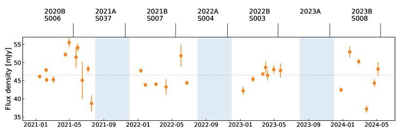
Figure 1: SMA Lightcurve at 230 GHz. Blue shaded areas mark the unobservable part of each year, where the NGC 5044 is too close to the sun or nighttime observations are not possible.

Our new data reveals intriguing results for the time variability and the spectral energy distribution (SED) of the central SMBH in NGC 5044. We first present our findings on the mm-lightcurve (section 3.1) and the derived periodogram analysis (section 3.2), and link this for a time-consistent SED in section 3.3.

3.1 The lightcurve at mm-wavelengths

A change in the mm continuum flux was first noticed in ALMA data taken in different epochs and configurations (Schellenberger et al., 2020b). Our new observations of 3.5 years of SMA monitoring observations of NGC 5044 allow us to analyze the mm variability at 230 GHz (flux meausrements are listed in Tab. A2) which we present in Fig. 1. The uncertainties of the individual flux measurements are typically between 0.5 and 1 mJy, which was the requirement of the proposed observations. However, on several observing days the achieved noise was highly affected by weather/opacity, the unavailability of particular antennae owing to engineering work, and/or the standard flux calibrators being unavailable (see Tab. A1). Observations on these days have larger uncertainties. Whenever observations were completely unusable they were usually repeated by the SMA staff in a timely manner. Soon after the start of our monitoring program in the first half of 2021 we find a peak in the lightcurve as the flux increases by 20% from the baseline level of about 46 mJy to about 55 mJy within a few months. By mid 2021 the flux appears to be back to the baseline level, before NGC 5044 becomes unobservable. After the observations restart in 2022 we find that another peak might have just been missed as we detect the tail of the peak with decreasing fluxes from 48 mJy to a consistent baseline until late June 2022 of 44 mJy. The outlier in early June 2022 (above 50 mJy) could be associated with a short peak that could only have lasted 2.5 months or less. The 2023 lightcurve does not include any strong peak, but contains measurements with $5-10\%$ lower fluxes than the previously assumed baseline. It is possible that a dip in the lightcurve in late 2021 is missed due to the sampling. Finally, our findings for the first half of 2024 indicate a very disturbed lightcurve with variability on a 1 to 2 month scale.

The SMA lightcurve covers the time of our VLA measurements (see section 2.2), and the ALMA 170 GHz measurements (project 2021.1.00766.S, PI Rose), which allows us to rescale these other instruments to a common time.

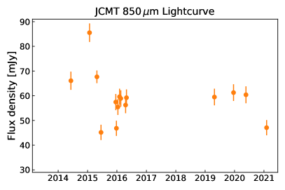
Figure 2: JCMT lightcurve at $850\text{\,}\mu\mathrm{m}$ (353 GHz).

We present the JCMT $850\text{\,}\mu\mathrm{m}$ lightcurve in Fig. 2 with measurements between 2014 and 2021. The sampling is highly uneven, with, for example, 6 measurements within 5 months around 2016 and no observation in the following 3 years. The overall scatter is 22%, and we see a slight downturn in 2021, where there is overlap with SMA data at 230 GHz.

3.2 Periodogram

We are able to derive statistical properties from the mm-lightcurves of NGC 5044 beyond the results presented in the previous section. A complication is posed by sparsely and unevenly sampled lightcurves which are set by the SMA observations, despite the efforts to have an approximate monthly cadence. The shortest sampled timescales are on the order of a few days, corresponding to frequencies $\sim$3\text{\times}{10}^{-1}\text{\,}\mathrm{d}\mathrm{a}\mathrm{y}^{-1}$$, while the longest time intervals are a few years, corresponding to frequencies $\sim${10}^{-3}\text{\,}\mathrm{d}\mathrm{a}\mathrm{y}^{-1}$$. We generally do not expect variability on timescales shorter than the light crossing time of the inner region of the accretion disk, which is a few Scharzschild radii (corresponding to several days).

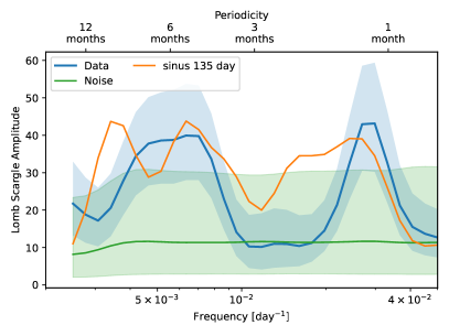
Figure 3: Lomb Scargle periodogram of the SMA lightcurve (blue). The green area shows the 1$\sigma$ random noise region, and the orange line the expected signal from a sine with 135 day period and the same observing mask as the SMA data.

The Lomb-Scargle periodogram, initially based on Lomb (1976); Scargle (1982), and with modifications by Press & Rybicki (1989); Zechmeister & Kürster (2009); Townsend (2010); VanderPlas (2018), is a standard tool for lightcurve analyses. We use the scipy implementation and apply the mean-subtraction (“precenter”). We note that, while the input requires angular frequencies ($\omega=\frac{2\pi}{T}$, where $T$ is the period of a periodic signal) we refer to normal frequency, $f=\frac{1}{T}$, in our interpretation and plots. The Lomb-Scargle periodogram was specifically designed to detect periodic signals in unevenly spaced observations. We utilize this tool and provide our SMA measurements as input. Figure 3 (blue line) shows the output periodogram when sampling frequencies between one week and 400 days: We visually identify two distinct peaks, one at around 6 months, and a second at 1.5 months. To understand the meaning of these peaks we create simulated signals based on a) a flat lightcurve (47 mJy) with a 22% Gaussian noise (observed scatter), and b) a superposition of a flat lightcurve ($47\text{\,}\mathrm{m}\mathrm{J}\mathrm{y}$), plus a sine signal with a 135 day period. We sample these models on a daily base for a 4 year timerange (January 2021 to January 2025) and use the actual 30 SMA observing days as a mask. We compute 1000 Lomb-Scargle periodograms from random realizations and analyze the 68% region around the median. For a) we find no periodicity and a flat signal (see green bar in Fig. 3), while for b) we find several peaks, two of which resemble the observations quite well (orange line in Fig. 3). This shows that due to the sparse lightcurve, it is possible that a periodic signal is causing the peaks that are observed, but it could also be explained by random noise since the significance of the blue line in Fig. 3 is small.

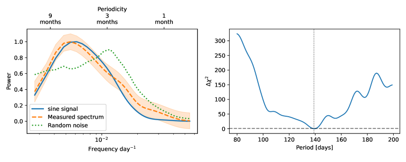
Figure 4: Left panel: Normalized power spectrum of the SMA lightcurve based on the Arevalo-method (orange), and from simulated data of random noise (green) and a sine with 140 day period (blue). Right panel: Illustrating the residuals ($\chi^{2}$) over a range of possible sine periods.

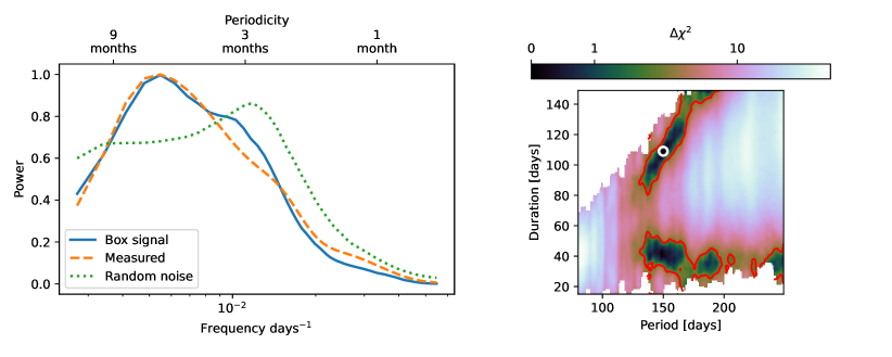
Figure 5: Left: As Fig. 4 but for a box signal. Right: The best-fit period is 150 days, and the duration is around 41/109 days, but poorly constrained.

Our second method to calculate the power of periodic signals in sparsely sampled data is based on the $\Delta$-variance method by Arévalo et al. (2012). This method has mostly been applied to determine the power spectra of fluctuations in two-dimensional surface brightness images with arbitrary masking (Zhuravleva et al., 2015; Romero et al., 2023, 2024; Dupourqué et al., 2024), but can be used for one-dimensional problems as well (as stated in Arévalo et al., 2012). This method introduces biases into the output spectra, but based on simple simulations we find that these mostly affect the upper and lower end of the frequencies, while we are looking for a signal that is well sampled with the SMA observational cadence. The concept stems from Parseval’s Theorem, which effectively equates the integral of the power spectrum to the integral of the variance. In effect, the difference of Gaussians (Mexican Hat) acts as a not-so narrow $\delta$ function whereby one can specify a frequency at which one can recover the power. The variance of this difference is proportional to the power of the frequency that was tested. We tested this method with simulated sine signal, and found a broadened Gaussian instead of a narrow delta function in the power spectrum. This broadening is expected and discussed in Arévalo et al. (2012), and does not prevent us from measuring a peak location. The orange dashed line in the left panels of Figures 4 and 5 shows the measured spectrum using this algorithm. The overall curve is very smooth, with a clear peak around 6 months, and some minor peak at 3 months. However, due to the biases and smoothing effects, we apply the method to simulated signals to reproduce our signal in the power spectrum. First, we use a simple sine with the same mask as the observations, and phase-shift it randomly. We test periods from 80 to 200 days, and calculate a $\chi^{2}$ from the difference between the observed power spectrum and the median of 100 randomly phase-shifted sine-functions. Note that we assume an uncertainty of 0.2 on the normalized power. We find a minimum $\chi^{2}$ around 140 days. Fig. 4 (right) shows the distribution of the $\chi^{2}$ after subtracting the minimum. The horizontal dashed line at $\Delta\chi^{2}=1$ indicates the $1\sigma$ uncertainty range. We find that a sine with $T=140^{+16}_{-29}\,$\mathrm{d}$$ describes the data reasonably well. The best fit sine-power spectrum is overplotted in Fig. 4 (left) in blue. For self-consistency we test a random noise signal, which when evenly sampled creates a flat line in the power spectrum. However, when applying the observing mask and selecting only the 30 days of SMA observations, we find that this random signal produces the green dotted line in Fig. 4 and 5 (left). Interestingly, this is no longer flat but features a peak around 3 months, falling toward zero at higher frequencies, but flattening at a higher level at lower frequencies. This explains the tail seen in the orange curve of Fig. 5 (left) at the same frequency. As a second test-model we use a box signal with a simple on/off periodic signal that has a specified duration. By design the duration has to be always smaller than the period. Since we have two free parameters (duration and period), we evaluate the $\chi^{2}$ on a grid, each time phase-shifting the function randomly. We show the $\chi^{2}$ results in Fig. 5 (left panel). The red contours indicate the $1\sigma$ region around the minimum $\chi^{2}$, where $\Delta\chi^{2}=2.3$. We find a best-fit period of $150^{+16}_{-29}$ days, in agreement with the period of the sine. However, the duration of $109_{-10}^{+69}$ days is poorly constrained. The $\chi^{2}$ image in Fig. 5 (left) can be seen as a 2D likelihood function, which shows some symmetry: For a period $p$ (with $p\gtrsim$109\text{\,}\mathrm{d}$$ and duration $d<p/2$ it appears to be equally likely to have the duration $p-d$, which is simply the inverted version of the signal. Since we have a random test signal (green curve) which represents our null hypothesis, and we can quantify the likelihood distribution $\mathcal{L}_{H_{0}}$ that the noise power spectrum is an adequate representation of the measured power spectrum (orange). We can further quantify the test likelihood $\mathcal{L}_{H_{1}}$ of the sine or box model’s power spectrum being a good representation of the observed spectrum. While $\mathcal{L}_{H_{1}}$ is very peaked at a particular probability, $\mathcal{L}_{H_{0}}$ is very broad. We find that in only 2.2% (11.7%) of all cases the noise model is a better representation than the box (sine) model. This means we can reject the hypothesis of the SMA lightcurve being random at more than $2\,\sigma$.

While the Lomb-Scargle test does not allow one to robustly distinguish between a variable signal and random noise, we see hints of variability with period of 4 to 6 months. Interestingly, the Arevalo-method shows that the the lightcurve is most likely a periodic (box) signal with about 150 day period (about 5 months).

3.3 The Spectral Energy Distribution

A mm-upturn of the continuum fluxes in the central radio source in NGC 5044 was first noticed by David et al. (2014, 2017) when comparing ALMA 230 GHz data with lower frequency radio fluxes. Schellenberger et al. (2020a) have measured and modeled the SED of the radio continuum source in NGC 5044 from $\sim$200\text{\,}\mathrm{M}\mathrm{H}\mathrm{z}$$ to $600\text{\,}\mathrm{G}\mathrm{H}\mathrm{z}$, and concluded that the emission appears to be well parametrized by a jet model with a self absorption component, combined with an advection dominated accretion flow (ADAF) model. The combination of a jet and ADAF model has been applied to other Low Luminosity AGNs (LLAGN) and low-ionization nuclear emission-line region (LINER) AGN (Quataert et al., 1999; Nemmen et al., 2014; Wu et al., 2007; Xie et al., 2016; Yan et al., 2024), several of them in the vicinity of M87/Virgo.

Flux densities of the central radio source are listed in Schellenberger et al. (2020a) from Giant Metrewave Radio Telescope (GMRT), VLA, VLA Sky Survey (VLASS), ALMA and JCMT. However, the lack of reliable, recent measurements between 10 to $100\text{\,}\mathrm{G}\mathrm{H}\mathrm{z}$ added large uncertainties on some of the model parameters of the jet component. This gap is filled by our recent VLA K and Q band observations, and we also add more recent ALMA and JCMT data. The synergy of the mm-lightcurve and the SED is evident; our detailed mm-lightcurve allows us to “rectify” fluxes to a common epoch (Feb. 2021). The “corrected” SED can be fit with models to obtain parameters on feeding and feedback history, which in turn can be used to interpret the mm-variability in terms of the accretion history.

Our combined model consists of 12 parameters, which we describe here. Our ADAF emission model follows the description in Schellenberger et al. (2020a). The first parameter is the SMBH mass $M$, which was determined by David et al. (2009) through the Gebhardt et al. (2000) $M-\sigma$ scaling relation to be $2.3\text{\times}{10}^{8}\text{\,}\mathrm{M}_{\odot}$. However, Diniz et al. (2017) used a more recent relation (Kormendy & Ho, 2013) and a precisely measured velocity dispersion and concluded a SMBH mass of $1.8\text{\times}{10}^{9}\text{\,}\mathrm{M}_{\odot}$, which is over 7 times larger than the previous estimate used by Schellenberger et al. (2020a). We leave $M$ free to vary in our fit. The accretion rate, $\dot{M}$, is also left free in our fit and is expected to be low $\dot{M}<$0.1\text{\,}\mathrm{M}_{\odot}\,\mathrm{y}\mathrm{r}^{-1}$$. It can be compared with star formation rates and cooling rates (e.g., McDonald et al., 2018). Variability in the ADAF flux can most easily be explained by a changing accretion rate. The inner ADAF truncation radius, $r$, is set to $3R_{S}$, where $R_{S}=\frac{2GM}{c^{2}}$ is the Schwarzschild radius. The viscosity parameter, $\alpha$, is also fixed to $0.3$, which is typically used for ADAFs (Liu & Taam, 2013). The gas-to-total pressure $\beta$ can also be referred to as the magnetic parameter, since the total pressure is the sum of the gas and magnetic pressure, which gives the identity $\frac{p_{\rm mag}}{p_{\rm gas}}=\frac{1}{\beta}-1$, where $p_{\rm mag}=\frac{B^{2}}{8\pi}$. We typically use a fixed $\beta=0.5$, which means that the magnetic and gas pressure are equal, but also have a test-case where the magnetic pressure is negligible, $\beta=0.99$. The last ADAF parameter in our model is $\delta$, which quantifies the heat energy distribution between electrons and ions. $\delta$ is expected to be close to the mass ratio of electrons and protons $\delta\approx\frac{1}{1836}$, but we leave it free to vary with a normal prior centered at $\frac{1}{1836}$ and a $\sigma_{\delta}=$2\text{\times}{10}^{-4}$$.

For the jet emission model we use the synchrofit package (Turner, 2018; Turner et al., 2018), which contains routines to calculate synchrotron emission of an aging plasma following the JP approach (Jaffe & Perola, 1973), the KP formalism that does not include any electron pitch angle scattering (Kardashev, 1962; Pacholczyk & Roberts, 1971), and the Continuous Injection model (CI, Komissarov & Gubanov, 1994). All three models have basic parameters, such as a normalization $J_{0}$ (left free to vary), an injection spectral index $\alpha_{\rm inj}=\frac{s-1}{2}$, where $s$ is the spectral index of the energy distribution of electrons injected into the plasma, $N(E)dE\propto E^{-s}dE$, and is fixed to $s=2$ (see e.g., Carilli et al., 1991), and a break frequency $\nu_{\rm break}$. The CI model also has an additional parameter, $\kappa=\frac{T_{\rm off}}{\tau}$, that describes the fraction of time that the AGN is injecting energy into the plasma. Note that the JP and KP models do not have an active injection of “fresh” electrons, and describe the emission of an aging plasma which was injected at $t=0$. Lastly, the synchrotron self absorption (SSA) model (Blandford & Konigl, 1979; Rybicki & Lightman, 2008) contains only two parameters, the spectral index $\alpha_{\rm SSA}$ and the the break/turn-over frequency $\nu_{\rm SSA}$ between the optically thin and thick regime. Both SSA parameters have no priors. While for a perfectly optically thick plasma $\alpha_{\rm SSA}=-2.5$ is expected, shallower slopes have often been observed (e.g., Laor & Behar, 2008; Ishibashi & Courvoisier, 2011; Kim et al., 2021).

Table 1: SED Fitting results.

Run	Jet	$M$	$\dot{M}$	$\beta$	$\delta^{-1}$	$r$	$\nu_{\rm b}$	$\kappa=\frac{T_{\rm off}}{\tau}$	$\alpha_{\rm inj}$	$\log\mathcal{L}$
		${10}^{9}\text{\,}\mathrm{M}_{\odot}$	${10}^{-2}\text{\,}\frac{M_{\odot}}{yr}$			$R_{S}$	GHz
(1)	(2)	(3)	(4)	(5)	(6)	(7)	(8)	(9)	(10)	(11)
1	CI	$2.17^{+0.17}_{-0.13}$	$1.20^{+0.73}_{-0.33}$	$0.50$	$1832^{+1122}_{-490}$	$3.0$	$15.5^{+5.9}_{-5.1}$	$0.78^{+0.16}_{-0.27}$	$0.50$	$-38.98$
2	CI	$0.28^{+0.32}_{-0.13}$	$9.59^{+7.80}_{-5.10}$	$0.50$	$1741^{+910}_{-467}$	$32.8^{+35.0}_{-19.2}$	$14.8^{+6.0}_{-4.9}$	$0.78^{+0.16}_{-0.27}$	$0.50$	$-39.78$
3	CI	$1.34^{+0.24}_{-0.17}$	$0.02^{+0.07}_{-0.01}$	$0.50$	$37^{+103}_{-23}$	$3.0$	$15.6^{+6.1}_{-5.3}$	$0.78^{+0.16}_{-0.28}$	$0.50$	$-39.02$
4	CI	$2.93^{+0.23}_{-0.21}$	$37.63^{+14.68}_{-9.43}$	$0.99$	$1680^{+666}_{-402}$	$3.0$	$15.1^{+5.9}_{-5.0}$	$0.78^{+0.16}_{-0.27}$	$0.50$	$-39.07$
5	JP	$2.23^{+0.16}_{-0.13}$	$1.16^{+0.62}_{-0.31}$	$0.50$	$1821^{+976}_{-484}$	$3.0$	$20.1^{+5.3}_{-3.8}$		$0.50$	$-38.23$
6	KP	$2.23^{+0.16}_{-0.13}$	$1.16^{+0.61}_{-0.31}$	$0.50$	$1830^{+959}_{-489}$	$3.0$	$12.5^{+3.4}_{-2.4}$		$0.50$	$-41.39$
7	CI	$2.26^{+0.29}_{-0.15}$	$1.24^{+1.49}_{-0.38}$	$0.50$	$1962^{+2393}_{-584}$	$3.0$	$11.1^{+4.4}_{-2.6}$	$0.50$	$0.50$	$-42.97$
8	CI	$2.18^{+0.16}_{-0.12}$	$1.15^{+0.63}_{-0.30}$	$0.50$	$1837^{+990}_{-478}$	$3.0$	$5.1^{+2.1}_{-1.5}$	$0.00$	$0.50$	$-76.32$
9	JP	$2.23^{+0.16}_{-0.13}$	$1.15^{+0.61}_{-0.30}$	$0.50$	$1823^{+950}_{-472}$	$3.0$	$26.1^{+8.0}_{-5.8}$		$0.55$	$-39.64$
10	JP	$2.24^{+0.16}_{-0.13}$	$1.15^{+0.59}_{-0.31}$	$0.50$	$1816^{+929}_{-480}$	$3.0$	$10.6^{+4.8}_{-2.5}$		$0.31^{+0.11}_{-0.12}$	$-35.82$
11	JP	$2.25^{+0.17}_{-0.13}$	$1.15^{+0.64}_{-0.32}$	$0.50$	$1806^{+1010}_{-491}$	$3.0$	$40.6^{+3.2}_{-5.3}$		$0.75$	$-48.09$

Note. — Column (1) gives a reference number for the fitting run, as referred to in the text. Column (2) names the jet emission model that is employed (acronyms see text). ADAF model parameters are listed in columns (3) to (7), the SMBH mass (3), the mass accretion rate (4), the gas to total pressure (5), the inverse of the heat energy distribution between electrons and ions (6), and the inner truncation radius (7). Columns (8) to (10) refer to the jet emission model, specifically the break frequency (8), the remnant fraction which only applies to the CI case (9), and the injection spectral index (10). Column (11) states the log of the likelihood as a measure for the goodness of fit. Parameters without uncertainties are fixed to their stated values.

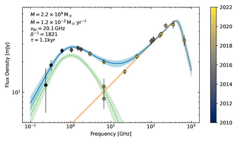
Figure 6: SED fit of our best fit JP Model (Run 5 in Tab. 1). The combined model is shown in blue, the self-absorbed jet model in green, and the ADAF model in orange. The two lower datapoints at 6.7 GHz are the VLBA flux measurements of the compact and extended emission. The color scale of the datapoints shows the year when the observation was taken.

We use the emcee package (Goodman & Weare, 2010; Foreman-Mackey et al., 2013) to sample the posterior distribution of the MCMC. We run a total of 11 fits with different initial conditions, and list our results in Table 1.

• Run 1 is a Continuous Injection jet model with all parameters set to their default priors. In this case the we find a mass $M$ that is only marginally larger than the one observed by Diniz et al. (2017), a relatively low accretion rate consistent with expectations and star formation rates, and break frequency between 10 to 20 GHz. While $\kappa$ is listed with a median value of $0.78$, we note that in all cases where $\kappa$ is free (Runs 1-4) the posterior distribution is strongly skewed toward 1, which means the fit clearly favors a CI model that is off all the time (i.e., an AGN which has ceased to power its jets).

• Run 2 is like 1 but has no prior on truncation radius $r$, which interestingly results in a much larger $r$, but also a mass $M$ that is close to the old value from David et al. (2009). The accretion rate in Run 2 is about 8 times larger than in 1, but closer to the star formation rate stated in Werner et al. (2014).

• Run 3 is like 1 but has a uniform instead of normal prior on the ion/electron energy distribution parameter $\delta$. This causes $\delta$ to move to a value much closer to equal heat distribution between ions and electrons, and at the same time forces the accretion rate to be almost 2 orders of magnitude lower.

• Run 4 is like 1 but has a minimal magnetic field pressure, meaning the magnetic field $B$ is 10 times lower. This increases the accretion rate by a factor of 30, which is unlikely since the star formation rate is very low (Werner et al., 2014).

• Run 5 is like 1 but uses a JP jet model instead of a CI model. Differences are small, since $\kappa$ in the CI model 1 is very close to $\kappa=1$ anyway. The break frequency is slightly larger, mostly due to the fact that the AGN is now off 100% of the time. Despite having fewer free parameters (no $\kappa$) the likelihood is highest (with the exception of Run 10), and we mark this our default result and show it in Fig. 6.

• Run 6 is like 1 but uses a KP jet model instead of a CI model. This case is very similar to the JP model from Run 5, but has a significantly lower break frequency. However, the likelihood is also worse, and therefore we favor the JP model over the KP.

• Runs 7/8 are like 1 but have a fixed $\kappa$ to 0.5 / 0, meaning the AGN is active powering the jets half the time/all the time. While this is similar to the model explored by Schellenberger et al. (2020a), our additional data, especially the VLA K and Q band measurements, clearly disfavor these models. The lower break frequency tries to compensate for the more active state of the AGN.

• Runs 9/10/11 are like the standard JP case (Run 5) but with a different injection spectral index, $\alpha_{\rm inj}=0.55$ (Run 9), $\alpha_{\rm inj}=0.75$ (Run 11), and $\alpha_{\rm inj}$ free to vary (Run 10). Again, the data disfavors a steeper spectral index, and the fit tries to compensate through a much higher break frequency. In Run 10 however, the best fit injection index is around 0.3, which is shallower than expected. While this marks the highest likelihood, we do not think that a injection index of 0.3 is physical, and the fit is likely driven by the lower value of the VLA K band observation.

4 Discussion and outlook

The information provided by the SED models allows us to further extract intrinsic properties of the central region near the AGN that are linked to the feeding and feedback processes. Despite the recently launched, small scale jets discovered by Schellenberger et al. (2020a) our SED fitting does not confirm that the AGN is actively powering jets at the moment. A continuous injection of particles into the jets, especially at a high duty cycle (small $\kappa$) has been clearly rejected (see Tab. 1, Run 8). Instead the jet emission is consistent with an aging plasma as frequently observed in radio lobes. We can adopt the estimate for the magnetic field strength in the jets from Schellenberger et al. (2020a) of $B=$4.7\text{\,}\mathrm{m}\mathrm{G}$$, which was derived assuming energy equipartition (Govoni & Feretti, 2004; Giacintucci et al., 2008). The magnetic field strengths allows us compute the aging time (see Turner et al., 2018),

$$\tau=\frac{vB^{0.5}}{B^{2}+B_{\rm IC}^{2}}\left[\nu_{b}(1+z)\right]^{-0.5}~{},$$ (1)

where $\nu_{b}$ is the break frequency, $B_{\rm IC}=0.317(1+z)^{2}\,$\mathrm{n}\mathrm{T}$$, and the constant $v=\left(\frac{243\pi m_{\rm e}^{5}c^{2}}{4\mu_{0}^{2}e^{7}}\right)^{0.5}$. For Run 5 which is our default case, we derive a timescale $\tau=$1.1\pm 0.1\text{\,}\mathrm{k}\mathrm{y}\mathrm{r}$$. The break frequency is somewhat correlated with the injection spectral index, and therefore we get the most extreme values for the timescale in Run 10 and 11, where the injection index is either 0.3 ($\tau=$1.5\pm 0.3\text{\,}\mathrm{k}\mathrm{y}\mathrm{r}$$) or 0.75 ($\tau=$0.8\pm 0.1\text{\,}\mathrm{k}\mathrm{y}\mathrm{r}$$). Therefore, it is safe to conclude that the AGN has stopped injecting electrons into the jets. The fact that this timescale is very different from the ADAF variability (1000 years vs. months) illustrates that the processes that launch jets are unrelated to the “smaller” feeding events of the black hole from surrounding cold gas (e.g., Schellenberger et al., 2020b). While in principle one could determine the magnetic field from the SSA turnover around 5 GHz (see e.g., Marscher, 1983; Kim et al., 2021), uncertainties on the size of the absorbed core region dominate the results, which renders it impossible to even give an order of magnitude estimate (the size enters with the 4 power). However, we believe the magnetic field on the order of mG is a realistic estimate of the average magnetic field along the $\sim$parsec jets (O’Sullivan & Gabuzda, 2010; Kim et al., 2021).

VLBA data has shown that a compact core with an inverted spectrum is located between the jets (Schellenberger et al., 2020a). Our ADAF model provides an accurate description of the SED up to sub-mm wavelengths. Since the inverted spectrum is due to synchrotron emission one can derive the magnetic field within the ADAF emission region (Mahadevan, 1997). For our default model (Run 5) we find a magnetic field of $B_{\rm ADAF}=$870\text{\,}\mathrm{G}$$, about $200\,000$ times larger than in the jets. It has been pointed out before that magnetic fields in accretion disks have to be 100 s of G to launch jets (see Blandford & Payne, 1982; Jafari, 2019). For almost all Runs (Tab. 1) we find magnetic fields strengths in the ADAF emission region of 800 to $900\text{\,}\mathrm{G}$, with the exception of Run 2, 3 and 4: Run 2 has an almost 10 times smaller SMBH mass, and a much larger disk truncation, and if the magnetic field increases towards the center of the AGN, the average field will be smaller, in this case $339^{+165}_{-110}\,$\mathrm{G}$$. Run 3 has an extremely low accretion rate, which implies the low magnetic field of $151^{+122}_{-50}\,$\mathrm{G}$$. Run 4 has a high accretion rate (about 2000 times higher than run 3) but the magnetic pressure was set to be only 1%, and the two effects almost balance each other, leading to a magnetic field of $578^{+92}_{-68}\,$\mathrm{G}$$.

If we want to precisely quantify the truncation radius $r$, which is tightly linked to other parameters in our fit, such as the SMBH mass, we need to have accurate measurements at even shorter wavelengths. It turns out that at wavelengths shorter than $450\text{\,}\mathrm{\SIUnitSymbolMicro m}$ (JCMT SCUBA2) the difference between models of Run 1 and 2 becomes very clear: While at lower frequencies the difference is minimal, at $1\text{\,}\mathrm{T}\mathrm{H}\mathrm{z}$ or $300\text{\,}\mathrm{\SIUnitSymbolMicro m}$ the larger truncation radius (Run 2, with the smaller SMBH mass) has a 50% larger flux than Run 1 (16.6 vs. $25.2\text{\,}\mathrm{m}\mathrm{J}\mathrm{y}$). This regime was accessible with Herschel.

The lightcurve variability in NGC 5044 was reported previously, but our SMA observations have now quantified the level of variability. A 22% overall scatter with a baseline around $45\text{\,}\mathrm{m}\mathrm{J}\mathrm{y}$ is significantly larger than the typical fractional uncertainty of the measurements of $\lesssim 2\%$. At the beginning of our program in 2021 we observed a $\sim 3$ month peak in the lightcurve, characterized by an increase from 45 to $55\text{\,}\mathrm{m}\mathrm{J}\mathrm{y}$. If we assume that changes in the accretion rate are the sole cause for this increase, it means that the ADAF accretion rate rose by 50% to $1.74\text{\times}{10}^{-2}\text{\,}\mathrm{M}_{\odot}\,\mathrm{y}\mathrm{r}^{-1}$. Our box model also predicts a duration of the signal of about 100  days (or around 50 days, which is equivalent for a period of 150 days), similar to what was observed in the first peak. We can convert the typical variability timescale into a physical length, which yields $\sim 350\,R_{\rm S}$ ($0.08\text{\,}\mathrm{p}\mathrm{c}$ or $0.5\text{\,}\mathrm{m}\mathrm{a}\mathrm{s}$). This size is reasonable for the ADAF emitting accretion disk, and it is possible to resolve these scales with VLBA imaging at K/Q band (Schellenberger et al. in prep).

While the Lomb-Scargle and the Arevalo tests in section 3.2 reveal a periodicity, we have too limited dataset to infer that the detected variability originates from a periodic process. However, we have demonstrated that the variability is real and has a characteristic timescale of $\sim$150 days, which is not explained by just random noise combined with our sparse sampling of the lightcurve. Results on the existence of Quasi-periodic oscillations (QPO) in X-ray lightcurves of AGN have been controversial and a random walk noise (Brownian noise) as alternative interpretation appears more likely (e.g., Press, 1978; MacLeod et al., 2010; Kelly et al., 2009; Krishnan et al., 2021; Rueda et al., 2022). A random walk noise, also known as red noise, is characterized by a power spectrum with a slope of $-2$. We do not see a power law in the Arevalo power spectrum, and we confirmed that an input powerlaw-spectrum signal combined with a mask that follows our SMA observing schedule, will produce a powerlaw spectrum. In order to clearly characterize a truly periodic process that causes the observed variability, we will need a larger dataset with a similar sampling over several more years.

While an ADAF-like spectrum has been observed in several sources, group central galaxies with their strong cooling and shallower gravitational potential than large clusters, mark a special class. Although the mm emission in the central AGN in NGC 5044 is well described by an ADAF model, the suitability has to be demonstrated for more cases. If the ADAF model turns out to be a common paradigm for the cooling and AGN feeding process, the overall feedback model can be linked from cold, infalling material, to large scale outflows and cavities (e.g., Morganti, 2017; Eckert et al., 2021). Our ongoing SMA program to search for other ADAFs in group central galaxies starts from a small sample of selected galaxy groups with a wide range of properties (cool-core, relaxed, disturbed, CO rich), and has already confirmed an ADAF spectrum in NGC 5084 (Schellenberger et al., in prep.). This X-ray faint but high richness group hosts an S0 central galaxy with a radio point source and a large HI disk. However, no CO is detected (see Kolokythas et al., 2022; O’Sullivan et al., 2018). In many aspects NGC 5084 is very different from NGC 5044. Further observations leading to potentially more detections in other groups will allow linking this radiatively inefficient accretion model to the cooling gas and the broader feedback process.

5 Summary

We presented results from our recent SMA monitoring observations of the central continuum source in NGC 5044, and our VLA K and Q band, as well as archival JCMT observations. With an angular distance of only 31 Mpc this system is ideal to study AGN feedback on the galaxy group scale. The mm-wavelength time variability has been proposed in the past, but it has never been studied in a systematic way so it can be linked to the feeding process of the AGN. Based on past SED fits this system was known host an AGN in ADAF mode, but with our new data we were able to quantify important parameters to better precision than previously. Our findings are as follows.

• Our new SMA data undoubtedly demonstrates the mm-variability of the NGC 5044 continuum source over a 3 year timescale with measurements on monthly cadence whenever the source was observable. We find a baseline flux of $46\text{\,}\mathrm{m}\mathrm{J}\mathrm{y}$ and an overall 22% variability. We were able to identify distinct peaks in the lightcurve, such as the 20% increase in early 2021.

• We provide a statistical analysis of the lightcurve variability that takes into account the sparse and unequal sampling, and find consistency with a periodic signal of the order of 150 days.

• Based on the lightcurve we “correct” fluxes from other instruments for the SED fitting, which is well represented by a jet model (JP with SSA) and an AGN ADAF model. We are able to constrain the break frequency of the jet emission, which implies that the jet plasma is about $1\text{\,}\mathrm{k}\mathrm{y}\mathrm{r}$ old, and no longer powered by the AGN. A continuous injection with an active AGN was ruled out. The SMBH mass derived from the ADAF model is consistent with recent estimates, and the accretion rate is in line with expectations. The magnetic field pressure in the ADAF emission region is significant, on the same order of the gas pressure.

• With a few assumptions we are able to quantify the magnetic field in the jets ($4.7\text{\,}\mathrm{m}\mathrm{G}$) and the accretion disk ($\sim$870\text{\,}\mathrm{G}$$). Based on the observed variability we can estimate the ADAF disk diameter to about $0.08\text{\,}\mathrm{p}\mathrm{c}$ or $0.5\text{\,}\mathrm{m}\mathrm{a}\mathrm{s}$, which can be resolved by high frequency VLBA observations.

The rich multiwavelength dataset available for NGC 5044 makes this source unique, and allows us to push our understanding of the accretion and feedback process in galaxy groups. Our analysis and results show how complex AGN/feedback processes are, with a broader parameter space to be explored, i.e. longer lightcurve sampling, observations at higher frequencies, and a thorough comparison to other detected ADAFs in central group galaxies.

Appendix A Tables

In this section we list all supplemental information, such as observation times and setups. Table A1 lists the SMA observations, and Tab. A2 the corresponding flux densities. Table A3 shows the JCMT observations.

Table A1: SMA monitoring observations of NGC 5044

SMA	Date	Observation	On-source	#Ant.	Flux Cal	Band Cal	Receiver
project	M/D/Y	[h:mm]	[h:mm]				[GHz]
(1)	(2)	(3)	(4)	(5)	(6)	(7)	(8)
2020B-S006	01/15/2021	4:00	2:26	7	Vesta	3C279	211–221, 231–241
	02/07/2021	3:27	2:41	7	Vesta	3C279	207–217, 221–251
	02/09/2021	6:15	2:31	7	Vesta	3C279	211–221, 231–241
	03/05/2021	3:47	2:41	7	Vesta	3C279	210–221, 230–241
	04/17/2021	2:36	1:28	6	Vesta	3C279	205–215, 225–235
	04/30/2021	4:03	2:55	6	Vesta	3C279	211–229, 231–249
	05/25/2021	8:31	4:52	5	Vesta	3C279	210–220, 230–240
	05/31/2021	2:28	1:44	6	Vesta	3C279	211–229, 231–249
2021A-S037	06/16/2021	3:48	2:13	6	Vesta	3C279	225–267
	07/07/2021	3:12	2:12	6	Vesta	3C279	220–230, 240–250
	07/19/2021	3:51	2:41	6	Vesta	3C279	211–221, 231–241
2021B-S007	01/11/2022	5:24	3:25	6	Ceres	3C279	211–221, 231–241
	01/27/2022	4:48	3:25	6	Vesta	1743-038	211–221, 231–241
	03/06/2022	4:08	3:14	5	Vesta	1159+292	211–221, 231–241
	04/11/2022	3:19	1:57	6	Ceres	3C279	220–230, 240–250
	06/03/2022	2:40	0:44	6	Ceres	3C279	210–220, 230–240
2022A-S004	06/24/2022	4:25	2:55	6	Titan	BL Lac	210–220, 230–240
2022B-S003	01/11/2023	7:20	4:23	6	Ceres	3C279	211–221, 231–241
	02/15/2023	5:53	3:24	5	Ceres	3C279	211–221, 231–241
	03/22/2023	6:30	4:24	6	Ceres	3C279	211–221, 231–241
	04/01/2023	5:57	4:07	6	Ceres	3C279	205–215, 225–235
	04/08/2023	9:39	6:34	6	Ceres	3C279	210–221, 230–241
	04/30/2023	9:26	6:34	6	Ceres	3C279	211–221, 231–241
	05/24/2023	9:00	4:52	5	Ceres	3C279	211–221, 231–241
2023B-S008	12/26/2023	4:19	2:49	6	Pallas	3C279	210–251
	01/26/2024	5:43	3:54	7	Ceres	3C279	211–221, 231–241
	02/27/2024	2:19	1:32	6	Ceres	3C84	210–220, 230–275
	03/26/2024	6:47	3:11	7	Pallas	3C279	211–221, 231–241
	04/23/2024	4:16	1:44	5	Ceres	BL Lac	210–220, 230–240
	05/06/2024	3:48	2:04	7	Vesta	3C279	211–221, 231–241

Note. — Column (1) is the SMA project/proposal numbers and semesters, column (2) lists the observing date, columns (3) and (4) state the total and on-target observing time, respectively. The active number of antenna during the observation is listed in column (5), and the flux and bandpass calibration sources are given in columns (6) and (7), respectively. Column (8) gives the frequency of the sidebands.

Table A2: SMA 230 GHz fluxes of NGC 5044

Date	Flux	Flux Error		Date	Flux	Flux Error		Date	Flux	Flux Error
Y-M-D	mJy	mJy		Y-M-D	mJy	mJy		Y-M-D	mJy	mJy
(1)	(2)	(3)		(1)	(2)	(3)		(1)	(2)	(3)
2021-01-15	46.15	0.58		2021-07-19	38.72	2.23		2023-04-01	38.72	1.61
2021-02-07	47.94	0.58		2022-01-11	47.77	0.58		2023-04-08	47.77	1.39
2021-02-09	45.21	0.64		2022-01-27	43.85	0.51		2023-04-30	43.85	1.11
2021-03-05	45.29	0.95		2022-03-06	44.02	0.49		2023-05-24	44.02	1.95
2021-04-17	52.21	0.64		2022-04-11	43.28	2.15		2023-12-26	43.28	0.60
2021-04-30	55.52	1.23		2022-06-03	51.84	3.04		2024-01-26	51.84	1.50
2021-05-25	51.49	2.89		2022-06-24	44.41	0.59		2024-02-27	44.41	0.75
2021-05-31	54.11	1.07		2023-01-11	42.24	1.09		2024-03-26	42.24	0.97
2021-06-16	45.10	5.12		2023-02-15	45.42	0.78		2024-04-23	45.42	1.09
2021-07-07	48.26	0.97		2023-03-22	46.86	0.51		2024-05-06	46.86	1.86

Note. — For each observing date (1) we list the measured SMA fluxes (2) and uncertainties (3).

Table A3: Archival JCMT Observations of NGC 5044

Project	Date	Exposure	Flux 850$\mu\mathrm{m}$		Project	Date	Exposure	Flux 850$\mu\mathrm{m}$
		850/450$\mu\mathrm{m}$	mJy				850/450$\mu\mathrm{m}$	mJy
(1)	(2)	(3)	(4)		(1)	(2)	(3)	(4)
S14AU03	2014-06-08	1.1/0.3min	$66.1\pm 3.7$		M16AP083	2016-02-02	2.9/0.7min	$59.6\pm 3.3$
S14BU03	2015-01-25	1.1/0.3min	$85.5\pm 3.7$			2016-02-17	2.8/0.7min	$58.9\pm 3.3$
M15AI70	2015-04-27	1.2/0.3min	$67.7\pm 2.6$			2016-04-17	2.8/0.7min	$56.2\pm 3.3$
	2015-06-17	1.5/0.4min	$45.2\pm 3.1$			2016-04-28	2.8/0.7min	$59.2\pm 3.3$
M15BI025	2015-12-17	2.9/0.7min	$57.5\pm 3.3$		M19AP054	2019-04-26	2.9/0.7min	$59.5\pm 3.4$
	2015-12-25	2.9/0.7min	$46.8\pm 3.1$		M19BP038	2019-12-19	2.8/0.7min	$61.3\pm 3.4$
	2016-01-12	2.9/0.7min	$55.5\pm 3.2$		M20AP043	2020-05-22	2.9/0.7min	$60.4\pm 3.4$
					E21AK006	2021-02-02	2.9/0.7min	$47.1\pm 3.1$

Note. — We list the JCMT projects (1), the observation date (2), effective exposure times for the two frequencies (3), and the flux measurement including the uncertainty (4).

References

- Arévalo et al. (2012) Arévalo, P., Churazov, E., Zhuravleva, I., Hernández-Monteagudo, C., & Revnivtsev, M. 2012, Mon. Not. R. Astron. Soc., 426, 1793
- Ball et al. (2011) Ball, N. M., Schade, D., & Astronomy Data Centre, C. 2011, in American Astronomical Society Meeting Abstracts, Vol. 217, American Astronomical Society Meeting Abstracts #217, 344.03
- Blandford & Konigl (1979) Blandford, R. D., & Konigl, A. 1979, Astrophys. J., 232, 34
- Blandford & Payne (1982) Blandford, R. D., & Payne, D. G. 1982, MNRAS, 199, 883
- Blanton et al. (2003) Blanton, E. L., Sarazin, C. L., & McNamara, B. R. 2003, Astrophys. J.
- Burke et al. (2023) Burke, D., Laurino, O., wmclaugh, et al. 2023, sherpa/sherpa: Sherpa 4.15.1, Zenodo
- Böhringer et al. (1993) Böhringer, H., Voges, W., Fabian, A. C., & others. 1993, Mon. Not. R. Astron. Soc., 264, L25
- Carilli et al. (1991) Carilli, C. L., Perley, R. A., Dreher, J. W., & Leahy, J. P. 1991, ApJ, 383, 554
- Chapin et al. (2013) Chapin, E. L., Berry, D. S., Gibb, A. G., et al. 2013, Mon. Not. R. Astron. Soc., 430, 2545
- Churazov et al. (2000) Churazov, E., Forman, W., Jones, C., & Böhringer, H. 2000, Astron. Astrophys, 356, 788
- David et al. (2009) David, L. P., Jones, C., Forman, W., et al. 2009, ApJ, 705, 624
- David et al. (2017) David, L. P., Vrtilek, J., O’Sullivan, E., et al. 2017, ApJ, 842, 84
- David et al. (2014) David, L. P., Lim, J., Forman, W., et al. 2014, Astrophys. J., 792, 94
- Dempsey et al. (2013) Dempsey, J. T., Friberg, P., Jenness, T., et al. 2013, Mon. Not. R. Astron. Soc., 430, 2534
- Diniz et al. (2017) Diniz, S. I. F., Pastoriza, M. G., Hernandez-Jimenez, J. A., et al. 2017, Mon. Not. R. Astron. Soc., 470, 1703
- Donea et al. (1999) Donea, A. C., Falcke, H., & Biermann, P. L. 1999, in Astronomical Society of the Pacific Conference Series, Vol. 186, The Central Parsecs of the Galaxy, ed. H. Falcke, A. Cotera, W. J. Duschl, F. Melia, & M. J. Rieke, 162
- Dupourqué et al. (2024) Dupourqué, S., Clerc, N., Pointecouteau, E., et al. 2024, Astron. Astrophys., 687, A58
- Eckert et al. (2021) Eckert, D., Gaspari, M., Gastaldello, F., Le Brun, A. M. C., & O’Sullivan, E. 2021, Universe, 7, 142
- Fabian et al. (1984) Fabian, A. C., Nulsen, P. E. J., & Canizares, C. R. 1984, Nature, 310, 733
- Fabian et al. (2003) Fabian, A. C., Sanders, J. S., Allen, S. W., et al. 2003, Mon. Not. R. Astron. Soc., 344, L43
- Falcke & Biermann (1999) Falcke, H., & Biermann, P. L. 1999, Astron. Astrophys., 342, 49
- Foreman-Mackey et al. (2013) Foreman-Mackey, D., Hogg, D. W., Lang, D., & Goodman, J. 2013, Publ. Astro. Soc. Pac., 125, 306
- Forman et al. (2007) Forman, W., Jones, C., Churazov, E., et al. 2007, Astrophys. J., 665, 1057
- Fruscione et al. (2006) Fruscione, A., McDowell, J. C., Allen, G. E., et al. 2006, in Observatory Operations: Strategies, Processes, and Systems, ed. D. R. Silva & R. E. Doxsey (SPIE)
- Gebhardt et al. (2000) Gebhardt, K., Bender, R., Bower, G., et al. 2000, Astrophys. J., 539, L13
- Giacintucci et al. (2008) Giacintucci, S., Vrtilek, J. M., Murgia, M., et al. 2008, ApJ, 682, 186
- Goodman & Weare (2010) Goodman, J., & Weare, J. 2010, Comm. App. Math. Comp. Sci., 5, 65
- Govoni & Feretti (2004) Govoni, F., & Feretti, L. 2004, Int. J. Mod. Phys. D, 13, 1549
- Grimes et al. (2020) Grimes, P., Blundell, R., Leiker, P., et al. 2020, in Proceedings of the 31st International Symposium on Space Terahertz Technology, 60–66
- Grimes et al. (2024) Grimes, P. K., Keating, G. K., Blundell, R., et al. 2024, arXiv [astro-ph.IM 2406.17192]
- Gurwell et al. (2007) Gurwell, M. A., Peck, A. B., Hostler, S. R., & others. 2007, ASP Conference Series: From Z-Machines to ALMA, 375
- Holland et al. (2013) Holland, W. S., Bintley, D., Chapin, E. L., et al. 2013, Mon. Not. R. Astron. Soc., 430, 2513
- Ishibashi & Courvoisier (2011) Ishibashi, W., & Courvoisier, T. J.-L. 2011, Astron. Astrophys., 525, A118
- J. Hazelton et al. (2017) J. Hazelton, B., C. Jacobs, D., C. Pober, J., & P. Beardsley, A. 2017, J. Open Source Softw., 2, 140
- Jafari (2019) Jafari, A. 2019, arXiv [astro-ph.HE 1904.09677]
- Jaffe & Perola (1973) Jaffe, W. J., & Perola, G. C. 1973, Astron. Astrophys.
- Kaneda et al. (2008) Kaneda, H., Onaka, T., Sakon, I., et al. 2008, ApJ, 684, 270
- Kardashev (1962) Kardashev, N. S. 1962, SvA, 6, 317
- Kelly et al. (2009) Kelly, B. C., Bechtold, J., & Siemiginowska, A. 2009, Astrophys. J., 698, 895
- Kim et al. (2021) Kim, S.-H., Lee, S.-S., Lee, J. W., et al. 2021, Mon. Not. R. Astron. Soc., 510, 815
- Kolokythas et al. (2022) Kolokythas, K., Vaddi, S., O’Sullivan, E., et al. 2022, Mon. Not. R. Astron. Soc., 510, 4191
- Komissarov & Gubanov (1994) Komissarov, S. S., & Gubanov, A. G. 1994, Astron. Astrophys.
- Kormendy & Ho (2013) Kormendy, J., & Ho, L. C. 2013, Annu. Rev. Astron. Astrophys., 51, 511
- Krishnan et al. (2021) Krishnan, S., Markowitz, A. G., Schwarzenberg-Czerny, A., & Middleton, M. J. 2021, Mon. Not. R. Astron. Soc., 508, 3975
- Laor & Behar (2008) Laor, A., & Behar, E. 2008, Mon. Not. R. Astron. Soc., 390, 847
- Liu & Taam (2013) Liu, B. F., & Taam, R. E. 2013, Astrophys. J. Suppl. Ser., 207, 17
- Lomb (1976) Lomb, N. R. 1976, Astrophys. Space Sci., 39, 447
- MacLeod et al. (2010) MacLeod, C. L., Ivezić, Z., Kochanek, C. S., et al. 2010, ApJ, 721, 1014
- Mahadevan (1997) Mahadevan, R. 1997, ApJ, 477, 585
- Mairs et al. (2021) Mairs, S., Dempsey, J. T., Bell, G. S., et al. 2021, Astron. J., 162, 191
- Marscher (1983) Marscher, A. P. 1983, ApJ, 264, 296
- McDonald et al. (2018) McDonald, M., Gaspari, M., McNamara, B. R., & Tremblay, G. R. 2018, ApJ, 858, 45
- McMullin et al. (2007) McMullin, J. P., Waters, B., Schiebel, D., Young, W., & Golap, K. 2007, in Astronomical Society of the Pacific Conference Series, Vol. 376, Astronomical Data Analysis Software and Systems XVI, ed. R. A. Shaw, F. Hill, & D. J. Bell, 127
- McNamara et al. (2000) McNamara, B. R., Wise, M., Nulsen, P. E., et al. 2000, Astrophys. J., 534, L135
- Morganti (2017) Morganti, R. 2017, Front. Astron. Space Sci., 4, 309944
- Narayan et al. (1998) Narayan, R., Mahadevan, R., & Quataert, E. 1998, in Theory of Black Hole Accretion Disks, ed. M. A. Abramowicz, G. Björnsson, & J. E. Pringle, 148–182
- Nemmen et al. (2014) Nemmen, R. S., Storchi-Bergmann, T., & Eracleous, M. 2014, Mon. Not. R. Astron. Soc., 438, 2804
- O’Sullivan et al. (2018) O’Sullivan, E., Combes, F., Salomé, P., et al. 2018, Astron. Astrophys. Suppl. Ser., 618, A126
- O’Sullivan & Gabuzda (2010) O’Sullivan, S. P., & Gabuzda, D. C. 2010, in Astronomical Society of the Pacific Conference Series, Vol. 427, Accretion and Ejection in AGN: a Global View, ed. L. Maraschi, G. Ghisellini, R. Della Ceca, & F. Tavecchio, 207
- Pacholczyk & Roberts (1971) Pacholczyk, A. G., & Roberts, J. A. 1971, Phys. Today, 24, 57
- Pavlovski & Pope (2009) Pavlovski, G., & Pope, E. C. D. 2009, Mon. Not. R. Astron. Soc., 399, 2195
- Perley & Butler (2017) Perley, R. A., & Butler, B. J. 2017, ApJS, 230, 7
- Pope (2007) Pope, E. C. D. 2007, Mon. Not. R. Astron. Soc., 381, 741
- Press (1978) Press, W. H. 1978, Comments Astrophys., 7, 103
- Press & Rybicki (1989) Press, W. H., & Rybicki, G. B. 1989, ApJ, 338, 277
- Primiani et al. (2016) Primiani, R. A., Young, K. H., Young, A., et al. 2016, J. Astron. Instrum., 05, 1641006
- Quataert et al. (1999) Quataert, E., Di Matteo T, Narayan, R., & Ho, L. C. 1999, Astrophys. J., 525, L89
- Randall et al. (2010) Randall, S. W., Forman, W. R., Giacintucci, S., et al. 2010, ApJ, 726, 86
- Romero et al. (2023) Romero, C. E., Gaspari, M., Schellenberger, G., et al. 2023, Astrophys. J., 951, 41
- Romero et al. (2024) —. 2024, Astrophys. J., 970, 73
- Rueda et al. (2022) Rueda, H., Glicenstein, J.-F., & Brun, F. 2022, Astrophys. J., 934, 6
- Rybicki & Lightman (2008) Rybicki, G. B., & Lightman, A. P. 2008, Radiative Processes in Astrophysics (John Wiley & Sons)
- Scargle (1982) Scargle, J. D. 1982, Astrophys. J., 263, 835
- Schellenberger et al. (2020a) Schellenberger, G., David, L. P., Vrtilek, J., et al. 2020a, ApJ, 906, 16
- Schellenberger et al. (2020b) —. 2020b, ApJ, 894, 72
- Stern et al. (2019) Stern, J., Fielding, D., Faucher-Giguère, C.-A., & Quataert, E. 2019, Mon. Not. R. Astron. Soc., 488, 2549
- The CASA Team et al. (2022) The CASA Team, Bean, B., Bhatnagar, S., et al. 2022, Publ. Astron. Soc. Pac., 134, 114501
- Tonry et al. (2001) Tonry, J. L., Dressler, A., Blakeslee, J. P., et al. 2001, Astrophys. J., 546, 681
- Townsend (2010) Townsend, R. H. D. 2010, Astrophys. J. Suppl. Ser., 191, 247
- Turner (2018) Turner, R. J. 2018, Mon. Not. R. Astron. Soc., 476, 2522
- Turner et al. (2018) Turner, R. J., Shabala, S. S., & Krause, M. G. H. 2018, Mon. Not. R. Astron. Soc., 474, 3361
- Ubertosi et al. (2024) Ubertosi, F., Schellenberger, G., O’Sullivan, E., et al. 2024, Astrophys. J., 961, 134
- VanderPlas (2018) VanderPlas, J. T. 2018, Astrophys. J. Suppl. Ser., 236, 16
- Voit & Donahue (2011) Voit, G. M., & Donahue, M. 2011, Astrophys. J. Lett., 738, L24
- Werner et al. (2018) Werner, N., McNamara, B. R., Churazov, E., & Scannapieco, E. 2018, Space Sci. Rev., 215, 5
- Werner et al. (2014) Werner, N., Oonk, J. B. R., Sun, M., et al. 2014, Mon. Not. R. Astron. Soc., 439, 2291
- Wu et al. (2007) Wu, Q., Yuan, F., & Cao, X. 2007, Astrophys. J., 669, 96
- Xie et al. (2016) Xie, F.-G., Zdziarski, A. A., Ma, R., & Yang, Q.-X. 2016, Mon. Not. R. Astron. Soc., 463, 2287
- Yan et al. (2024) Yan, X., Lu, R.-S., Jiang, W., et al. 2024, Astrophys. J., 965, 128
- Yuan et al. (2002) Yuan, F., Markoff, S., & Falcke, H. 2002, Astron. Astrophys., 383, 854
- Yuan & Narayan (2014) Yuan, F., & Narayan, R. 2014, Annu. Rev. Astron. Astrophys., 52, 529
- Zechmeister & Kürster (2009) Zechmeister, M., & Kürster, M. 2009, Astron. Astrophys., 496, 577
- Zhuravleva et al. (2015) Zhuravleva, I., Churazov, E., Arévalo, P., et al. 2015, Mon. Not. R. Astron. Soc., 450, 4184